Nilpotent symmetries as a mechanism for Grand Unification

Abstract

In the classic Coleman–Mandula no-go theorem which prohibits the unification of internal and spacetime symmetries, the assumption of the existence of a positive definite invariant scalar product on the Lie algebra of the internal group is essential. If one instead allows the scalar product to be positive semi-definite, this opens new possibilities for unification of gauge and spacetime symmetries. It follows from theorems on the structure of Lie algebras, that in the case of unified symmetries, the degenerate directions of the positive semi-definite invariant scalar product have to correspond to local symmetries with nilpotent generators. In this paper we construct a workable minimal toy model making use of this mechanism: it admits unified local symmetries having a compact ($\mathrm{U}(1)$) component, a Lorentz ($\mathrm{SL}(2,\mathbb{C})$) component, and a nilpotent component gluing these together. The construction is such that the full unified symmetry group acts locally and faithfully on the matter field sector, whereas the gauge fields which would correspond to the nilpotent generators can be transformed out from the theory, leaving gauge fields only with compact charges. It is shown that already the ordinary Dirac equation admits an extremely simple prototype example for the above gauge field elimination mechanism: it has a local symmetry with corresponding eliminable gauge field, related to the dilatation group. The outlined symmetry unification mechanism can be used to by-pass the Coleman–Mandula and related no-go theorems in a way that is fundamentally different from supersymmetry. In particular, the mechanism avoids invocation of super-coordinates or extra dimensions for the underlying spacetime manifold.

1 Introduction

One of the most important programmes in modern physics is concerned with model building in particle physics. Much of this endeavor is focused on the search for symmetries of Lagrangian field theories, and their corresponding quantum field theories. The Lagrangian of the Standard Model (SM) is essentially determined, up to a number of coupling constants, by its local symmetry group. The presence of a large number of free parameters reduces the predictive power of a physical theory, and for this reason it has been a long standing question whether it is possible to find alternatives to the Standard Model with a reduced number of free parameters by enlarging the local symmetry group. The ensemble of symmetries becomes the most restrictive whenever they form a non-direct product (unified) group. This simple principle motivated the gauge–gauge and gauge–spacetime symmetry unification strategies, which are sometimes referred to as GUT (Grand Unified Theories) and ToE (Theories of Everything). The early no-go theorem by McGlinn McGlinn1964 , the classic QFT no-go theorem by Coleman and Mandula ColemanMandula1967 , as well as the Poincaré group extension classification theorem by O’Raifeartaigh LOR1965a ; LOR1965b strongly restrict the possibilities for gauge–spacetime type unification. After the invention of supersymmetry (SUSY) SS1974 ; FZW1974 ; Ferrara1987 , it was widely believed that only that concept may provide a loophole to these no-go theorems HLS1975 . This is, however, only true under a certain set of assumptions.

It turns out that the primary ingredients of the above restrictive no-go theorems come from the general structural theory of finite dimensional Lie algebras, and mainly not from field theory itself, as discussed in Laszlo2017 , Section 2, and the Appendix A. Detailed study Weinberg2000 of the arguments of the above no-go theorems McGlinn1964 ; ColemanMandula1967 reveal that in order to obtain these prohibitive results, the assumption that the Lie algebra of the internal symmetry group admits a positive definite invariant scalar product is essential. That is, the above no-go theorems only follow automatically when the group of internal symmetries is assumed to be purely compact. In a previous paper Laszlo2017 it was demonstrated that whenever the assumption on this scalar product is somewhat weakened, by e.g. allowing it to be merely positive semi-definite, then a loophole opens. Under the semi-definiteness assumption, the internal group may not only be purely compact, but can also contain nilpotent generators. Since the nilpotent generators may carry compact and Lorentz charges as well, a gauge–spacetime type symmetry unification becomes group-theoretically possible. The main point of the present paper is to construct a minimal workable toy model utilizing this group-theoretical loophole.

The requirement of compactness of the internal symmetry group in conventional gauge theories has several motivations: (i) compact Lie groups are classified and their representation theory is well understood, (ii) the Standard Model gauge group ${\mathrm{U}(1){\times}\mathrm{SU}(2){\times}\mathrm{SU}(3)}$ is compact, and (iii) Yang–Mills fields with compact gauge group admit a strictly positive definite energy functional. In the more general case when an internal Lie algebra with merely positive semi-definite invariant scalar product is considered, it follows that besides the gauge fields with compact charges, some gauge fields with nilpotent charges occur, and these have vanishing Yang–Mills kinetic Lagrangian. Correspondingly, they have zero Yang–Mills kinetic energy term. This clearly raises the question of whether gauge fields with such kind of charges are acceptable from a physical point of view: how should one interpret a field theory with gauge field degrees of freedom, in which the gauge fields all possess non-negative energy density, as usual, but there are some unusual modes of the Yang–Mills fields which have zero kinetic energy? Surely these “exotic” components of the gauge fields cannot have an Euler–Lagrange equation similar to a conventional Yang–Mills equation, since they do not have a kinetic term.

In this paper we present a workable example of a unified local symmetry group of the above kind, along with a corresponding toy model, where the above type gauge fields with “exotic” (nilpotent) charges, necessary for a gauge–spacetime type symmetry unification, can be transformed out from the Lagrangian. This gauge field elimination mechanism is due to a shift symmetry of the Lagrangian (see Section 5, following Eq.(56)). Therefore, in the resulting field theory, the full unified symmetry group acts locally and faithfully on the matter fields, but only the compact part of the internal symmetries has corresponding physical gauge fields. The matter field sector, on the other hand, behaves as usual in gauge theory, since it has a non-degenerate kinetic term.

The above mentioned fact, that there exists a Lagrangian with a local symmetry without corresponding gauge field, is quite striking, and at a first glance it might seem that such a theory must be very artificial. In Section 3, however, we show that already the ordinary Dirac kinetic Lagrangian, when viewed in appropriate field variables, does admit an extremely simplified version of the above gauge field elimination mechanism, related to the dilatation group.

In Section 4 we construct the above mentioned unified structure group of our toy model, involving compact ($\mathrm{U}(1)$), Lorentz ($\mathrm{SL}(2,\mathbb{C})$), and nilpotent generators, and then in Section 5 we constuct a corresponding invariant Lagrangian, with eliminable nilpotent gauge fields. It is seen that the proposed symmetry unification mechanism allows for nilpotent generators, and therefore may seem distantly analogous to SUSY. The main difference is, however, that the base manifold of the constructed model is the ordinary 4-dimensional Lorentzian spacetime, without super-coordinates or other extra dimensional objects.

In Section 6 we show that at the classical level the constructed Lagrangian has a single independent coupling constant. Finally, in Section 7 we present our conclusions.

The paper is closed by Appendix A, reviewing the structural theory of generic Lie algebras (not necessary semisimple), and some recent results concerning that in more details. These are relevant for applications of Lie algebra theory in model building.

2 Structural theorems for Lie groups and Lie algebras

Whenever some particle field theory has a classical field theory limit, one has a firm mathematical handle on the notion of its symmetry generators: the generators of the continuous symmetries of the theory are smooth vector fields on some kind of a total space of fields of the theory, which respect certain mathematical structures associated to the model. The spacetime manifold can be thought of, at least locally, as an immersed submanifold in the total space. Important information on the Lie algebra of these symmetry generating vector fields of the total space is present in the first order factor Lie algebra, carrying information about their formal Taylor expansion around a point of the spacetime manifold. In a classical field theory, by construction, this first order Lie algebra is always a finite dimensional real Lie algebra. Therefore, in this section we recall some facts about the structure of finite dimensional real Lie algebras Onishchik1990 ; IseTakeuchi1991 ; Jacobson1962 ; Snobl2014 that we shall need to discuss for model building in physics (see Appendix A for more details).

For a relativistic physical theory based on fields without internal structure, one can argue that the generators of first order local symmetries $\mathfrak{e}$ must be the Poincaré Lie algebra $\mathfrak{p}$. For fields with internal structure it is of interest to consider extensions of the Poincaré Lie algebra, i.e. Lie algebras $\mathfrak{e}$ with an injective homomorphism ${i:\,\mathfrak{p}\rightarrow\mathfrak{e}}$, and the investigation of such extensions has been an important strategy of modern particle physics. For example, the local symmetry algebra of the Standard Model is of the form ${\mathfrak{e}=\mathfrak{p}\oplus\mathfrak{u}(1){\oplus}\mathfrak{su}(2){\oplus}\mathfrak{su}(3)}$, which in particular splits as a direct sum.

The strategy known as unification aims at finding a field theoretical description of particle physics with a unified local symmetry group, i.e. a group such that its Lie algebra $\mathfrak{e}$ does not admit a direct sum decomposition ${\mathfrak{e}=\mathfrak{i}\oplus\mathfrak{c}}$ (see a detailed review on a large class of such models in Krasnov2018 ). As an example of a unified extension of the Poincaré group, we mention the conformal Poincaré group, with Lie algebra isomorphic to $\mathfrak{so}(2,4)$, which is a simple Lie algebra.

With these remarks in mind, we shall now recall the properties of extensions of the Poincaré Lie algebra, and start by recalling an important general result on the structure of Lie Algebras (see Appendix A for a more didactic and detailed treatment).

The Levi–Mal’cev decomposition theorem Snobl2014 ; Onishchik1990 ; IseTakeuchi1991 ; Jacobson1962 states that any finite dimensional real Lie algebra $\mathfrak{e}$ admits a semi-direct sum decomposition of the form

$$\mathfrak{e} = \mathop{\mathrm{rad}}\nolimits(\mathfrak{e})\mathbin{\hbox to0.0pt{$\Leftcircle$\hss}{+}}\mathfrak{l}$$ (1)

where $\mathop{\mathrm{rad}}\nolimits(\mathfrak{e})$ is the maximal solvable ideal in $\mathfrak{e}$, called to be the radical, and $\mathfrak{l}$ is the maximal semisimple Lie sub-algebra of $\mathfrak{e}$, called to be the Levi factor, which is unique up to inner automorphisms. The radical has a further important Lie sub-algebra, the nilradical denoted by $\mathop{\mathrm{nil}}\nolimits(\mathfrak{e})$, which is the maximal nilpotent ideal of $\mathfrak{e}$. The importance of the nilradical in gauge theory model building is justified by the fact that the elements of $\mathop{\mathrm{nil}}\nolimits(\mathfrak{e})$ are precisely the nilpotent symmetry generators, and that ${\mathop{\mathrm{nil}}\nolimits(\mathfrak{e})=\{0\}}$ can hold if and only if the Killing form on $\mathfrak{e}$ is non-degenerate. As an example of the Levi–Mal’cev decomposition, it is instructive to consider the Lie algebra of the Poincaré group,

$$\mathfrak{p} = \mathfrak{t}\mathbin{\hbox to0.0pt{$\Leftcircle$\hss}{+}}\boldsymbol{\ell},$$ (2)

where the radical $\mathfrak{t}$, i.e. the translations, is in fact abelian, and coincides with the nilradical. As discussed in Laszlo2017 and the Appendix A, the Lie algebra of the super-Poincaré group can also be considered as an example to the Levi–Mal’cev decomposition, with a non-abelian, but two-step nilradical.

Based on the Levi–Mal’cev decomposition, the O’Raifeartaigh classification theorem LOR1965a ; LOR1965b states that if $\mathfrak{e}$ is a finite dimensional extension of the Poincaré Lie algebra, then one of the following three mutually exclusive cases must hold.

1. Trivial extension, i.e. ${\mathfrak{e}=\mathfrak{p}\oplus\left\{\text{some Lie algebra}\right\}}$.

2. Not (A), and the translation Lie algebra $\mathfrak{t}$ is embedded into the radical $\mathop{\mathrm{rad}}\nolimits(\mathfrak{e})$ of the enlarged Lie algebra, whereas the Lorentz Lie algebra $\boldsymbol{\ell}$ is embedded into one of the simple components of the Levi factor $\mathfrak{l}$ of the enlarged Lie algebra.

3. The entire Poincaré Lie algebra ${\mathfrak{p}=\mathfrak{t}{\mathbin{\hbox to0.0pt{$\Leftcircle$\hss}{+}}}\boldsymbol{\ell}}$ is embedded into one of the simple components of the Levi factor $\mathfrak{l}$ of the enlarged Lie algebra.

Remark 2.1.

The O’Raifeartaigh theorem makes it easy to understand the principle of the Coleman–Mandula no-go theorem, without invoking deep field theoretical notions and arguments. The Coleman–Mandula theorem ColemanMandula1967 has a number of explicit and implicit assumptions, of which the following two are most relevant for our purpose.

1. There exists a positive definite scalar product on the generators of the non-Poincaré part of the extended Lie algebra, which in finite dimensions implies that the extended part is purely compact, and therefore it is a direct sum of copies of $\mathfrak{u}(1)$ and a compact semisimple part.

2. No symmetry breaking is present.

Assumption (i) rules out case (B) of the O’Raifeartaigh theorem, while assumption (ii) rules out case (C). Thus, the only remaining possibility is case (A). (It is also useful to note that in the Coleman–Mandula theorem there is another important implicit assumption as well: it is assumed that symmetry generators preserve the one-particle Fock subspace. This prohibits symmetry generators possibly stepping on the Fock space hierarchy, which can eventually also be an important loophole.)

As noted in Laszlo2017 and the Appendix A, the case (B) of the O’Raifeartaigh theorem opens the Lie algebra theoretical backdoor for the existence of the super-Poincaré group (SUSY). Namely, when presented in appropriate variables, the SUSY algebra can be cast into the form of a finite dimensional real Lie algebra extension of the Poincaré Lie algebra, with nontrivial, two-step nilradical. It is also instructive to note that an example for case (C) is the conformal Poincaré Lie algebra, isomorphic to the simple Lie algebra $\mathfrak{so}(2,4)$.

If we restrict to relativistic field theories based on fields taking values in a vector bundle over a 4-dimensional spacetime, as is the case for the Standard Model, then there must be Lie algebra homomorphisms

$$\mathfrak{p}\overset{i}{\longrightarrow}\mathfrak{e}\overset{o}{\longrightarrow}\mathfrak{p}$$ (3)

such that ${o\circ i:\,\mathfrak{p}\rightarrow\mathfrak{p}}$ is the identity map, see Laszlo2017 ; Laszlo2018 . We shall call such extensions conservative. Conservative extensions can always be cast in the form ${\mathfrak{e}=\mathfrak{t}\mathbin{\hbox to0.0pt{$\Leftcircle$\hss}{+}}\mathfrak{g}}$, where $\mathfrak{g}$ is the Lie algebra of the structure group. In this paper, we construct a unified conservative extension of the Poincaré Lie algebra, along with a corresponding minimal toy model Lagrangian. We remark that for instance, the Lie algebra of the super-Poincaré group is not a conservative extension of the Poincaré Lie algebra Laszlo2017 ; Laszlo2018 : it does not admit a surjective homomorphism ${o:\,\mathfrak{e}\rightarrow\mathfrak{p}}$ as in Eq.(3), since it contains non-Poincaré generators whose commutator is a Poincaré generator. Neither are the symmetries of extra dimensional, Kaluza–Klein-like theories conservative, for the same reason.

Remark 2.2.

In model building one often invokes a Yang–Mills-like kinetic Lagrangian term, with the requirement that all gauge fields propagate. This requirement is satisfied if and only if the Lie algebra of the internal group has an invariant, non-degenerate scalar product. Such Lie algebras are called quadratic. Not all quadratic Lie algebras are classified as of now. An important sub-class of quadratic Lie algebras are the reductive ones, admitting faithful finite dimensional completely reducible representations, which are most commonly used in model building, and are always direct sums of copies of $\mathfrak{u}(1)$ and of simple Lie algebras. For instance, the Lie algebra of the Standard Model structure group, $\mathfrak{sl}(2,\mathbb{C})\oplus\mathfrak{u}(1){\oplus}\mathfrak{su}(2){\oplus}\mathfrak{su}(3)$, is reductive. A quadratic Lie algebra is compact if its invariant scalar product is positive definite. These are always reductive, and the Standard Model internal Lie algebra $\mathfrak{u}(1){\oplus}\mathfrak{su}(2){\oplus}\mathfrak{su}(3)$ provides an example. Thus, in traditional model building, which involves only reductive Lie algebras, the radical must vanish or be central (and hence abelian). Therefore due to the Levi–Mal’cev decomposition Eq.(1), nilpotent generators cannot play an important role in symmetry unification if only reductive Lie algebras are considered. The mechanism outlined in the present paper hinges on the idea of considering conservative Poincaré extensions. Due to the O’Raifeartaigh theorem, these have to carry a nontrivial nilradical, if they are indecomposable (unified).

3 A hidden symmetry of the general relativistic Dirac kinetic Lagrangian

In this section we recall a result from Laszlo2021 , namely a hidden symmetry of the general relativistic Dirac kinetic Lagrangian. It is shown that the Dirac kinetic Lagrangian is insensitive to the $\mathrm{D}(1)$ part of the spinor connection. That example serves as a prototype for the gauge field elimination mechanism, which will be crucial in the toy model presented in Section 4 and after.

In order to show the hidden symmetry, let us formally define the general relativistic Dirac kinetic Lagrangian Trautman2008 . We use Penrose abstract indices for the tangent bundle. Let $\mathcal{M}$ be a four dimensional real smooth manifold. Assume it to be non-compact, and to admit a Lorentz signature spin structure. Let ${(D(\mathcal{M}),\,\gamma_{a})}$ be a Lorentzian Dirac bispinor bundle over it, i.e. $D(\mathcal{M})$ is a complex vector bundle with four dimensional fibers, and ${\gamma_{a}:\,T(\mathcal{M})\rightarrow D(\mathcal{M}){\otimes}D^{*}(\mathcal{M})}$ is a pointwise real-linear vector bundle homomorphism, with the Clifford property against some Lorentz metric. That is, the existence of a Lorentz signature metric tensor field $g(\gamma)_{ab}$ on $\mathcal{M}$ is required, such that ${\gamma_{a}\gamma_{b}+\gamma_{b}\gamma_{a}=2\,g(\gamma)_{ab}}\,I$ holds. In this presentation the fundamental field is $\gamma_{a}$ and not $g(\gamma)_{ab}$. It is well known Trautman2008 , that covariant derivations $\nabla_{a}$ on the vector bundle $D(\mathcal{M})$ exist which are lifts of the unique Levi-Civita covariant derivation on $T(\mathcal{M})$ associated to $g(\gamma)_{ab}$. More concretely, these covariant derivations are defined by the property that they are compatible with the Clifford map $\gamma_{a}$, with the metric $g(\gamma)_{ab}$, and are torsion-free on $T(\mathcal{M})$. Such lifts of the Levi-Civita covariant derivations are uniquely determined, up to adding a complex valued covector field, which can be though of as a ${\mathrm{D}(1){\times}\mathrm{U}(1)}$ gauge potential. Given a Dirac bispinor bundle ${(D(\mathcal{M}),\,\gamma_{a})}$, there exists a compatible pointwise antilinear injective vector bundle homomorphism ${\accentset{\rule{5.60002pt}{0.8pt}}{(\cdot)}:D(\mathcal{M})\rightarrow D^{*}(\mathcal{M})}$, called the Dirac adjoint, which is uniquely determined up to a pointwise real smooth nonzero scaling field.

Let us fix a Dirac adjoint together with the Dirac bispinor bundle, so that we have ${(D(\mathcal{M}),\,\gamma_{a},\,\accentset{\rule{5.60002pt}{0.8pt}}{(\cdot)})}$ given. Then, the covariant derivations $\nabla_{a}$ compatible with these structures are unique, up to adding an imaginary valued covector field. That is, they form an affine space over the gauge potentials with $\mathrm{U}(1)$ charge. That ambiquity can be used to encode a $\mathrm{U}(1)$ internal charge of the Dirac fields. As such, $\nabla_{a}$ encodes a combined gravitational and $\mathrm{U}(1)$ gauge connection, acting on the Dirac fields, being smooth sections $\Psi$ of $D(\mathcal{M})$. Then, one can define the Dirac kinetic Lagrangian

$$\mathrm{L}_{\text{Dirac}}(\gamma,\Psi,\nabla\Psi) \quad:=\quad \mathrm{v}_{\gamma}\,\mathop{\mathrm{Re}}\nolimits\left(\,\accentset{\rule{5.60002pt}{0.8pt}}{\Psi}\,\gamma^{a}\,\mathrm{i}\nabla_{a}\Psi\right)$$ (4)

being a spacetime pointwise bundle morphism into the real volume forms. Here, $\mathrm{v}_{\gamma}$ denotes the volume form field uniquely associated to the spacetime metric subordinate to the Clifford map $\gamma_{a}$ and to a chosen fixed spacetime orientation. The action functional is then local integrals of the volume form Eq.(4) over the compact regions of the spacetime $\mathcal{M}$.

Consider now the Lagrangian Eq.(4) as part of a larger theory in which case the Clifford map $\gamma_{a}$ is also dynamical. Then, besides the $\mathrm{U}(1)$ internal charges of $\Psi$, one may assign an action of the $\mathrm{D}(1)$ group on the fields in the following way:

$$\left(\begin{array}[]{l}\Psi\cr\gamma_{a}\cr\nabla_{b}\end{array}\right) \;\overset{\text{\tiny$\Omega{\in}\mathbb{R}^{{}^{+}}$}}{\text{\large$\longmapsto$}}\; \left(\begin{array}[]{l}\Omega\!\!^{{}^{-\frac{3}{2}}}\;\Psi\cr\Omega\,\gamma_{a}\cr\nabla_{b}\end{array}\right),$$ (11)

which can be considered as a $\mathrm{D}(1)$ gauge transformation with a constant ${\Omega\in\mathbb{R}^{+}}$, and the Dirac Lagrangian Eq.(4) is evidently invariant to it. As it is well known, even more is true: the Dirac Lagrangian Eq.(4) is conformally invariant. This means that the positive scaling field ${\Omega{>}0}$ may be taken to be not necessarily constant, at the price of making the transformation rule only slightly more complicated:

$$\left(\begin{array}[]{l}\Psi\cr\gamma_{a}\cr\nabla_{b}\end{array}\right) \;\overset{\text{\tiny$\Omega{>}0\;$}}{\text{\large$\longmapsto$}}\; \left(\begin{array}[]{l}\Omega\!\!^{{}^{-\frac{3}{2}}}\;\Psi\cr\Omega\,\gamma_{a}\cr\nabla_{b}-\frac{1}{2}\left(\mathrm{i}\Sigma{}_{b}{}^{c}-\delta{}_{b}{}^{c}I\right)(\Omega\!\!^{{}^{-1}}\!\!\mathrm{d}_{c}\Omega)\end{array}\right),$$ (18)

where ${\Sigma_{ab}:=\frac{\mathrm{i}}{2}\left(\gamma_{a}\gamma_{b}-\gamma_{b}\gamma_{a}\right)}$ is the spin tensor. The transformation rule of the covariant derivation $\nabla$ comes from the requirement that its metricity, torsion and compatibility with the Clifford map be unaffected by the rescaling, which unambiguously determines the pertinent term. In the following we show that one can also endow the fields ${(\Psi,\,\gamma_{a},\,\nabla_{b})}$ with local $\mathrm{D}(1)$ charges in a different way, in which scenario the Dirac kinetic Lagrangian Eq.(4) manifests a hidden symmetry concerning the local $\mathrm{D}(1)$ rescaling, which is related to spacetime pointwise rescaling of the physical measurement units.

3.1 The measure line bundle

In the works of Matolcsi Matolcsi1993 and of Janys̆ka, Modugno, Vitolo Modugno2010 , a simple mathematical framework was proposed which formalizes the notion of physical dimensional analysis. In their formulation, the mathematical model of special relativistic spacetime is considered to be a triplet $(\mathcal{M},L,\eta)$, where $\mathcal{M}$ is a four dimensional real affine space (modeling the flat spacetime), $L$ is a one dimensional oriented vector space (modeling the one dimensional vector space of length values), and $\eta:\mathop{\vee}^{2}T\rightarrow\mathop{\otimes}^{2}L$ is the flat Lorentz signature metric (constant throughout the spacetime), where $T$ is the underlying vector space of $\mathcal{M}$ (“tangent space”). The key idea in that construction is that the field quantities, such as the metric tensor $\eta$, are not simply real valued, but they take their values in the tensor powers of the measure line $L$. Due to the one-dimensionality of $L$, it can be shown that all rational tensor powers of it makes sense as distinct vector spaces. Such a setting formalizes the physical expectation that quantities actually have physical dimensions (the metric carries length-square dimension in this case), and that quantities with different physical dimensions cannot be added since they reside in different vector spaces. It is seen that the technique of measure lines is nothing but the precise mathematical formulation of ordinary dimensional analysis in physics.

This formulation of dimensional analysis, although it may seem relatively obvious, nearly tautological idea at a first glance, becomes a powerful tool when applied in a general relativistic setting. Namely, let our spacetime manifold $\mathcal{M}$ be some four dimensional real manifold, and let $L(\mathcal{M})$ be a real oriented vector bundle over $\mathcal{M}$, with one dimensional fiber. The fiber of $L(\mathcal{M})$ over each point of $\mathcal{M}$ shall model the oriented vector space of length values, and the pertinent line bundle shall be called the measure line bundle, or line bundle of lengths. We do not assume anything more about the line bundle $L(\mathcal{M})$, and in particular, we do not assume that a preferred trivialization is given. Just as in Matolcsi1993 ; Modugno2010 , the field quantities shall carry certain tensor powers of $L(\mathcal{M})$.

For instance, considering the Dirac action discussed above, we assume that a Dirac field $\Psi$ is a section of the vector bundle

$$L^{{}^{-\frac{3}{2}}}(\mathcal{M})\mathbin{\otimes}D(\mathcal{M}),$$ (19)

where $D(\mathcal{M})$ is an ordinary (dimension-free) Dirac bispinor vector bundle. Similarly, one can assume that the spacetime metric $g_{ab}$ is a section of the vector bundle ${L^{2}(\mathcal{M})\mathbin{\otimes}\mathop{\vee}^{2}T^{*}(\mathcal{M})}$, and that the Clifford map $\gamma_{a}$ is a section of the vector bundle ${L(\mathcal{M})\mathbin{\otimes}T^{*}(\mathcal{M}){\otimes}D(\mathcal{M}){\otimes}D^{*}(\mathcal{M})}$. This differential geometrical formulation encodes the physical idea that quantities occurring in the field theory have physical dimensions, and that the units of measurements can only be a priori defined spacetime pointwise. In order to transport the unit length to different spacetime points, a connection on $L(\mathcal{M})$ must be specified. Therefore, to make sense of the covariant derivative ${\nabla_{a}\Psi}$ of a section $\Psi$ of Eq.(19), $\nabla_{a}$ must be understood as the joint covariant derivation of the usual Clifford connection on $D(\mathcal{M})$, and some connection on the line bundle of lengths $L(\mathcal{M})$, the two being naturally joined via the Leibniz rule. Since the natural structure group of the vector bundle $L(\mathcal{M})$ is $\mathrm{D}(1)$, one can think of this as assigning local $\mathrm{D}(1)$ gauge charges to $\Psi$ and $\gamma_{a}$ and also including a corresponding $\mathrm{D}(1)$ gauge field within $\nabla_{a}$.

When constructing the Lagrangian as a volume form valued bundle morphism, one should keep in mind that it must be dimension-free (carrying zero tensor powers of $L(\mathcal{M})$), since only pure volume forms may be integrated over a manifold without any further assumptions, so that the action functional can be defined. As such, with the above assignment of dimensions, our example Lagrangian for the Dirac kinetic term Eq.(4) indeed takes its values purely as section of ${\mathop{\wedge}^{{}^{{}_{\dim(\mathcal{M})}}}\!T^{*}(\mathcal{M})}$, i.e. as a pure volume form.

On the above fields $(\Psi,\,\gamma_{a},\,\nabla_{b})$, one finds that an ${L(\mathcal{M})\rightarrow L(\mathcal{M})}$ pointwise vector bundle automorphism acts by a smooth positive real valued field $\Omega$ over the spacetime manifold $\mathcal{M}$, i.e. via a local $\mathrm{D}(1)$ gauge transformation

$$\left(\begin{array}[]{l}\Psi\cr\gamma_{a}\cr\nabla_{b}\end{array}\right) \;\overset{\text{\tiny$\Omega{>}0\;$}}{\text{\large$\longmapsto$}}\; \left(\begin{array}[]{l}\Omega\!\!^{{}^{-\frac{3}{2}}}\;\Psi\cr\Omega\,\gamma_{a}\cr\Omega\!\!^{{}^{-\frac{3}{2}}}\,\nabla_{b}\,\Omega\!^{{}^{\frac{3}{2}}}=\nabla_{b}+\Omega\!\!^{{}^{-\frac{3}{2}}}\mathrm{d}_{b}\Omega\!^{{}^{\frac{3}{2}}}\end{array}\right).$$ (26)

As trivially seen, Eq.(4) is invariant to these, which means that the Lagrangian is invariant to the pointwise rescaling of the measurement unit of lengths, and not only to Eq.(18).

3.2 Connection shift invariance of the Dirac Lagrangian

An interesting observation, not yet emphasized in the literature, is that the Dirac Lagrangian Eq.(4) understood in such variables, has a further hidden symmetry: it is invariant to the choice of the measure line bundle connection. Quite naturally, a change in the $L(\mathcal{M})$ connection is uniquely described by an affine shift transformation ${\nabla_{a}\mapsto\nabla_{a}+C_{a}}$, where $C_{a}$ is a smooth real-valued covector field over the spacetime. Direct evaluation shows that the Dirac Lagrangian Eq.(4) is invariant with respect to such a shift transformation

$$\left(\begin{array}[]{l}\Psi\cr\gamma_{a}\cr\nabla_{b}\end{array}\right) \;\overset{\text{\tiny$C_{d}$}}{\text{\large$\longmapsto$}}\; \left(\begin{array}[]{l}\Psi\cr\gamma_{a}\cr\nabla_{b}\;+\;C_{b}\end{array}\right).$$ (33)

In other terms, one could say that the Dirac Lagrangian Eq.(4) is invariant with respect to the choice of a $\mathrm{D}(1)$ gauge connection. The physical meaning of this fact is that the Lagrangian is invariant to the choice of any parallel transport rule of measurement units throughout spacetime, which is an additional symmetry on top of the usual conformal invariance Eq.(18) or pointwise measurement unit rescaling invariance Eq.(26). It can be shown Laszlo2021 , that all the Standard Model kinetic terms, when viewed in such variables, admit this symmetry.

It is seen that due to the ${\nabla_{a}\mapsto\nabla_{a}+C_{a}}$ shift symmetry of the Lagrangian, $C_{a}$ being $\mathrm{D}(1)$ valued, the original ${\mathrm{D}(1){\times}\mathrm{U}(1)}$ internal symmetry group, acting locally and faithfully on the matter fields, gives rise to a gauge field only for the compact direction, i.e. with $\mathrm{U}(1)$ degrees of freedom only. In our more complex toy model in this paper, we will show that such a forgetting mechanism can also be invoked for larger internal groups, and even with non-direct product (unified) group structure. By construction, however, it follows that the generators of the local symmetries whose gauge fields can be eliminated in such a manner, must sit in an $\mathop{\mathrm{ad}}\nolimits$-invariant sub-Lie algebra. Because of that, the Levi–Mal’cev decomposition theorem leads to strong constraints on how local internal symmetry generators deprived of corresponding gauge bosons can accompany the usual ones.

4 The structure group of the proposed toy model

The toy model presented here will be a general relativistic spinorial (Dirac-like) classical field theory of a fermion particle, invariant to some local nilpotent symmetry generators in addition to the usual local symmetries. The mathematically simplest, i.e. lowest dimensional nonabelian nilpotent Lie algebra is the so-called Heisenberg Lie algebra with $3$ generators, denoted by $\mathfrak{h}_{3}$. The name Heisenberg Lie algebra of $\mathfrak{h}_{3}$ comes from the formal resemblance of its Lie algebra relations to the Heisenberg exchange relations: $\mathfrak{h}_{3}$ is spanned by three elements $q$, $p$ and $e$, the only nonvanishing bracket relation being ${[p,q]=K\,e}$ where $K$ is some nonzero real number. For different values of $K$ the instances of $\mathfrak{h}_{3}$ are naturally isomorphic to each-other, therefore one can fix the value of the constant $K$ to an arbitrary preferred nonzero real number. The complexified $3$-generator Heisenberg Lie algebra is denoted by $\mathfrak{h}_{3}(\mathbb{C})$, and that shall be the nilradical of our example group. The Lie group corresponding to $\mathfrak{h}_{3}(\mathbb{C})$ is denoted by $\mathrm{H}_{3}(\mathbb{C})$.

It is straightforward to check, that the Lie algebra ${\mathfrak{gl}(2,\mathbb{C})\equiv\mathfrak{u}(1){\oplus}\,\boldsymbol{\mathtt{d}}(1){\oplus}\,\mathfrak{sl}(2,\mathbb{C})}$ can act as outer derivations on $\mathfrak{h}_{3}(\mathbb{C})$, via linearly mixing the first two generators $q$ and $p$, while merely scaling the third generator $e$ with the trace. In fact, e.g. via the LieAlgebras Maple package Anderson2016 , one may verify that the Lie algebra of outer derivations of $\mathfrak{h}_{3}(\mathbb{C})$ is $\mathfrak{gl}(2,\mathbb{C})$. Thus, the largest indecomposable semi-direct sum Lie algebra with nilradical $\mathfrak{h}_{3}(\mathbb{C})$ is nothing but ${\mathfrak{h}_{3}(\mathbb{C})\mathbin{\hbox to0.0pt{$\Leftcircle$\hss}{+}}\mathfrak{gl}(2,\mathbb{C})}$. This Lie algebra is an indecomposable conservative unification of the compact $\mathfrak{u}(1)$ and of the Weyl Lie algebra ${\boldsymbol{\mathtt{d}}(1){\oplus}\,\mathfrak{sl}(2,\mathbb{C})}$, since one has

$$\mathfrak{h}_{3}(\mathbb{C})\mathbin{\hbox to0.0pt{$\Leftcircle$\hss}{+}}\mathfrak{gl}(2,\mathbb{C}) \equiv \mathfrak{h}_{3}(\mathbb{C})\mathbin{\hbox to0.0pt{$\Leftcircle$\hss}{+}}\big{(}\mathfrak{u}(1){\oplus}\,\boldsymbol{\mathtt{d}}(1){\oplus}\,\mathfrak{sl}(2,\mathbb{C})\big{)}.\qquad$$ (34)

The Lie group corresponding to the Lie algebra ${\mathfrak{h}_{3}(\mathbb{C})\mathbin{\hbox to0.0pt{$\Leftcircle$\hss}{+}}\mathfrak{gl}(2,\mathbb{C})}$ is the indecomposable, semi-direct product group ${\mathrm{H}_{3}(\mathbb{C})\rtimes\mathrm{GL}(2,\mathbb{C})}$. The key ingredient for the structure group of our toy model shall be that group. In order to construct the model, we first show that the above is a matrix group, i.e. has a faithful linear representation. Then, we will demonstrate that its lowest dimensional faithful linear representation, i.e. its defining representation, carries a quite natural field theoretical meaning.

In the following, we shall use the ordinary two-spinor calculus PR1984 ; Wald1984 , and in particular its variant which is most wide spread in general relativity (GR) literature. Fix an abstract two dimensional complex vector space $S$, i.e. $S\cong\mathbb{C}^{2}$. The space $S$ is called the two-spinor space or simply spinor space, and its dual space $S^{*}$ is called the co-spinor space. Their complex conjugate vector spaces are denoted by $\bar{S}$ and $\bar{S}^{*}$, respectively. In the Penrose abstract index notation PR1984 ; Wald1984 , elements of ${S,\,S^{*},\,\bar{S},\,\bar{S}^{*}}$ are denoted with upper index ($\xi^{A}$), lower index ($\xi_{A}$), primed upper index ($\bar{\xi}^{A^{\prime}}$), and primed lower index ($\bar{\xi}_{A^{\prime}}$) spinors, respectively, with the spinor indices being based on upper case latin letters. The symbol $T$ will denote a four dimensional real vector space (“tangent space”), with $T^{*}$ being its dual. As is common in the GR literature, Penrose abstract indices of elements of $T$ and $T^{*}$ are denoted with lower case latin letter upper ($t^{a}$) and lower ($t_{a}$) indices. As usual, the index symmetrization and antisymmetrization are be denoted by enclosing the indices in round ${}_{{}^{(\,)}}$ or square ${}_{{}^{[\,]}}$ brackets, respectively.

Let $\mathcal{A}$ be a complex Grassmann algebra with 2 generators ($\mathcal{A}\cong\Lambda(\mathbb{C}^{2})$), i.e. $\mathcal{A}$ an exterior algebra of a two-dimensional complex vector space without a fixed preferred $\mathbb{Z}$-grading. Whenever a preferred $\mathbb{Z}$-grading is chosen, then $\mathcal{A}$ may be identified as ${\mathcal{A}\equiv\Lambda(S^{*})}$, i.e. a spinorial representation of it can be given. Motivated by this, we shall call $\mathcal{A}$ the space of generalized co-spinors. (The convention that we are representing $\mathcal{A}$ as $\Lambda(S^{*})$ and not as e.g. $\Lambda(S)$ is merely a matter of convenience for the Penrose abstract index formalism.) Given an element ${a\in\mathcal{A}}$, denote by ${L_{a}\in\mathop{\mathrm{Lin}}\nolimits(\mathcal{A})}$ the linear operator of left multiplication by $a$ on $\mathcal{A}$. Since $\mathcal{A}$ is a four dimensional complex unital associative algebra, the group of its invertible elements can act on the space $\mathcal{A}$ via $L$. Denote by ${M(\mathcal{A})\subset\mathcal{A}}$ the so-called maximal ideal of $\mathcal{A}$, which happens to be the subspace of order at least one forms within $\mathcal{A}$. Then, all the invertible elements of $\mathcal{A}$ can be uniquely written as a nonzero complex number times $\exp(m)$, with some element ${m\in M(\mathcal{A})}$. Thus, the group action of the left multiplication by an invertible element of $\mathcal{A}$ on $\mathcal{A}$ can be uniquely written as a nonzero complex scaling times ${\exp(L_{m})\in\mathrm{GL}(\mathcal{A})}$ with ${m\in M(\mathcal{A})}$.

The group ${\{\exp(L_{m})\,|\,m\in M(\mathcal{A})\}}$ can be easily seen to be isomorphic to $\mathrm{H}_{3}(\mathbb{C})$. In order to show this fact, it is enough to see that the Lie algebra defined by ${\{L_{m}\,|\,m\in M(\mathcal{A})\}}$ is isomorphic to $\mathfrak{h}_{3}(\mathbb{C})$. That is most easily demonstrated by fixing some $\mathbb{Z}$-grading ${\mathcal{A}\equiv\mathop{\bigoplus}_{p=0}^{2}\Lambda_{p}}$, and then taking the unit element ${\mathds{1}\in\Lambda_{0}}$, and canonical generators ${a_{1},a_{2}\in\Lambda_{1}}$, with which the basis ${\{\mathds{1},a_{1},a_{2},a_{1}a_{2}\}}$ spans the algebra $\mathcal{A}$, whereas the basis ${\{a_{1},a_{2},a_{1}a_{2}\}}$ spans its maximal ideal $M(\mathcal{A})$. Since $\mathcal{A}$ was defined to be a Grassmann algebra with two generators, it directly follows from the Grassmann relations that the Lie algebra spanned by ${\{L_{a_{1}},L_{a_{2}},L_{a_{1}a_{2}}\}}$ has the same commutation relations as $\mathfrak{h}_{3}(\mathbb{C})$, and therefore ${L_{M(\mathcal{A})}\equiv\mathfrak{h}_{3}(\mathbb{C})}$, and correspondingly one has ${\exp(L_{M(\mathcal{A})})\equiv\mathrm{H}_{3}(\mathbb{C})}$. As a consequence, one has natural faithful linear representations of $\mathfrak{h}_{3}(\mathbb{C})$ and $\mathrm{H}_{3}(\mathbb{C})$ on the space $\mathcal{A}$.

On the algebra $\mathcal{A}$, the group ${\mathrm{GL}(2,\mathbb{C})\equiv\mathrm{GL}(S^{*})}$ also has a natural representation. That is because ${\mathrm{GL}(S^{*})}\equiv{\mathrm{GL}(\Lambda_{1})}\equiv{\mathrm{GL}(M(\mathcal{A})/M^{2}(\mathcal{A}))}$ describes the $\mathbb{Z}$-grading preserving algebra automorphisms of $\mathcal{A}$ Djokovic1978 . Therefore, one can construct the semi-direct product group ${\exp(L_{M(\mathcal{A})})\rtimes\mathrm{GL}(\Lambda_{1})}\equiv{\mathrm{H}_{3}(\mathbb{C})\rtimes\mathrm{GL}(2,\mathbb{C})}$, which then by construction has a natural faithful complex-linear representation on $\mathcal{A}$, which happens to be the defining representation, i.e. the smallest dimensional faithful linear representation of ${\mathrm{H}_{3}(\mathbb{C})\rtimes\mathrm{GL}(2,\mathbb{C})}$. The structure of the algebra $\mathcal{A}$ along with the natural action of the group ${\exp(L_{M(\mathcal{A})})\rtimes\mathrm{GL}(\Lambda_{1})}$ on $\mathcal{A}$ is illustrated in Figure 1.

(a)

(b)

(c)

 
 
(d) (e) (f) (g)
 
 
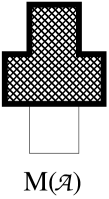
(h) (i) (j) (k)

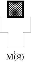
Figure 1: Illustration of the structure of the complex unital associative algebra ${\mathcal{A}\equiv\Lambda(S^{*})}$ and the natural group action of the conservative Lorentz group extension ${\exp(L_{M(\mathcal{A})})\rtimes\mathrm{GL}(\Lambda_{1})}$ over it. Panel (a): the algebra $\mathcal{A}$ with a fixed $\mathbb{Z}$-grading (${\Lambda_{p}\equiv\mathop{\wedge}^{p}S^{*}}$). Panel (b): whenever a fixed $\mathbb{Z}$-grading is taken, an element $\psi$ of $\mathcal{A}$ can be represented by a tuple of spinors. Panel (c): heuristically speaking, the algebra $\mathcal{A}$ can be considered as a creation operator algebra of fermions with 2 fundamental degrees of freedom. Panels (d)–(e)–(f)–(g): important subspaces of the algebra $\mathcal{A}$, namely the scalar sector $B(\mathcal{A})$, the maximal ideal $M(\mathcal{A})$, and its second power $M^{2}(\mathcal{A})$, moreover the center $Z(\mathcal{A})$. Panels (h)–(i): illustration of the group action of the grading preserving part ($\mathrm{GL}(\Lambda_{1})$) and of the grading non-preserving part ($\exp L_{M(\mathcal{A})}$) of the full symmetry group ${\exp(L_{M(\mathcal{A})})\rtimes\mathrm{GL}(\Lambda_{1})}$. The grading preserving part, by definition conserves the $p$-form subspaces, whereas the grading non-preserving part mixes higher forms to lower forms. Panels (j)–(k): list of all the invariant subspaces, which are invariant to the group action of the full symmetry group ${\exp(L_{M(\mathcal{A})})\rtimes\mathrm{GL}(\Lambda_{1})}$. It is seen that none of the invariant subspaces possess an invariant complementing subspace, and thus the defining representation on $\mathcal{A}$ is indecomposable. In other words: the pertinent group action puts $\mathcal{A}$ into a single multiplet. Note that in the representation space of a non-semisimple Lie group an invariant subspace might not have invariant complement, i.e. a reducible representation might still be an indecomposable (non-direct sum) multiplet.

Since the group ${\exp(L_{M(\mathcal{A})})\rtimes\mathrm{GL}(\Lambda_{1})}$ has a linear action on $\mathcal{A}$, there is a canonical faithful representation also on its complex conjugate space $\bar{\mathcal{A}}$, via the requirement of being compatible with the natural ${\mathcal{A}\rightarrow\bar{\mathcal{A}}}$ complex conjugation map. This is in analogy of $\mathrm{GL}(S^{*})$ having its canonical representation on $S^{*}$, and consequently having its canonical representation on $\bar{S}^{*}$, via requiring the invariance of the ${S^{*}\rightarrow\bar{S}^{*}}$ complex conjugation map.

The actual representation space in our toy model shall be ${A:=\bar{\mathcal{A}}\otimes\mathcal{A}}$, where $\otimes$ denotes ordinary, i.e. vector space sense tensor product (not a graded tensor product). The algebra $A$ is a kind of doubled exterior algebra, which we shall call spin algebra, being a 16 dimensional complex unital associative algebra. Since its components $\mathcal{A}$ and $\bar{\mathcal{A}}$ play the role of generalizations of the co-spinor space $S^{*}$ and the complex conjugate co-spinor space $\bar{S}^{*}$, the spin algebra ${A=\bar{\mathcal{A}}\otimes\mathcal{A}}$ can be considered as a generalization of the mixed co-spinor space $\bar{S}^{*}\otimes S^{*}$. In fact, whenever a preferred $\mathbb{Z}$-grading of $\mathcal{A}$ is fixed, the spin algebra may be identified as ${A\equiv\mathop{\bigoplus}_{p,q=0}^{2}\mathop{\wedge}^{p}\bar{S}^{*}\mathop{\otimes}\mathop{\wedge}^{q}S^{*}}$, i.e. its representation can be given in terms of ordinary two-spinors. By construction, the spin algebra $A$ also carries a natural antilinear involution ${\overline{(\cdot)}:A\rightarrow A}$, which we call charge conjugation, and which has the property ${\overline{x\,y}=\overline{x}\,\overline{y}}$ for all ${x,y\in A}$. The pertinent charge conjugation map is simply defined by the composition of the natural complex conjugation as a ${\bar{\mathcal{A}}\otimes\mathcal{A}\rightarrow\mathcal{A}\otimes\bar{\mathcal{A}}}$ map and of the natural tensor product swapping as a ${\mathcal{A}\otimes\bar{\mathcal{A}}\rightarrow\bar{\mathcal{A}}\otimes\mathcal{A}}$ map, hence giving rise to a natural ${\bar{\mathcal{A}}\otimes\mathcal{A}\rightarrow\bar{\mathcal{A}}\otimes\mathcal{A}}$ antilinear involution on $A$. It can be considered as a generalization of the hermitian conjugation ${\bar{S}^{*}\otimes S^{*}\rightarrow\bar{S}^{*}\otimes S^{*}}$ on the space of mixed co-spinors $\bar{S}^{*}\otimes S^{*}$, as usual in the ordinary two-spinor calculus. Since the group ${\exp(L_{M(\mathcal{A})})\rtimes\mathrm{GL}(\Lambda_{1})}\equiv{\mathrm{H}_{3}(\mathbb{C})\rtimes\mathrm{GL}(2,\mathbb{C})}$ has a natural linear representation both on $\mathcal{A}$ and $\bar{\mathcal{A}}$, it also has a corresponding linear representation on the spin algebra ${A=\bar{\mathcal{A}}\otimes\mathcal{A}}$.

The structure group of our toy model will be specified via its faithful linear representation on the spin algebra ${A=\bar{\mathcal{A}}\otimes\mathcal{A}}$. It is defined to be the group

$$\mathcal{G} \;\;:=\;\; \mathbb{C}^{{}^{\times}}\;\times\;\big{(}\,\exp(L_{M(\mathcal{A})})\;\rtimes\;\mathrm{GL}(\Lambda_{1})\,\big{)}$$ (35)

$$\;\;\;\;\equiv\;\; \Big{.}\mathbb{C}^{{}^{\times}}\;\times\;\big{(}\,\mathrm{H}_{3}(\mathbb{C})\;\rtimes\;\mathrm{GL}(2,\mathbb{C})\,\big{)}$$ (36)

$$\;\;\;\;\;\;\equiv\;\; \big{(}\,\mathbb{C}^{{}^{\times}}\;\times\;\mathrm{H}_{3}(\mathbb{C})\,\big{)}\;\rtimes\;\mathrm{GL}(2,\mathbb{C})$$ (37)

where $\mathbb{C}^{{}^{\times}}$ denotes the scaling by nonzero complex numbers on $A$. The factor $\mathbb{C}^{{}^{\times}}$ is merely present because in fact in the toy model, a projective representation of ${\exp(L_{M(\mathcal{A})})\rtimes\mathrm{GL}(\Lambda_{1})}\equiv{\mathrm{H}_{3}(\mathbb{C})\;\rtimes\;\mathrm{GL}(2,\mathbb{C})}$ is taken over $A$, and it is a notational convenience to view that projective representation instead a linear representation of $\mathcal{G}$ as in Eq.(37). The Lie algebra of $\mathcal{G}$ is correspondingly

$$\mathfrak{g} \;\;:=\;\; \mathbb{C}\;\oplus\;\Big{(}\,L_{M(\mathcal{A})}\;\mathbin{\hbox to0.0pt{$\Leftcircle$\hss}{+}}\;\mathfrak{gl}(\Lambda_{1})\,\Big{)}$$ (38)

$$\;\;\;\;\equiv\;\; \Big{.}\mathbb{C}\;\oplus\;\Big{(}\mathfrak{h}_{3}(\mathbb{C})\mathbin{\hbox to0.0pt{$\Leftcircle$\hss}{+}}\big{(}\mathfrak{u}(1){\oplus}\,\boldsymbol{\mathtt{d}}(1){\oplus}\,\mathfrak{sl}(2,\mathbb{C})\big{)}\Big{)}$$ (39)

$$\;\;\;\;\;\;\equiv\;\; \Big{.}\big{(}\mathbb{C}\oplus\mathfrak{h}_{3}(\mathbb{C})\big{)}\mathbin{\hbox to0.0pt{$\Leftcircle$\hss}{+}}\big{(}\mathfrak{u}(1){\oplus}\,\boldsymbol{\mathtt{d}}(1){\oplus}\,\mathfrak{sl}(2,\mathbb{C})\big{)}\qquad$$ (40)

where $\mathbb{C}$ denotes the scaling by complex numbers on $A$. The group $\mathcal{G}$ is invariant under the conjugation by elements of the charge conjugation group ${\{I,\,\overline{(\cdot)}\}\equiv\mathbb{Z}_{2}}$, where $I$ is the identity map on $A$. Therefore, the semi-direct product ${\mathcal{G}\rtimes\{I,\,\overline{(\cdot)}\}}$ is meaningful. This detail will be important because we will prescribe the charge conjugation group ${\{I,\,\overline{(\cdot)}\}\equiv\mathbb{Z}_{2}}$ to be global symmetry of the toy model. The structure of the spin algebra $A$ along with the natural action of the group ${\mathcal{G}\rtimes\{I,\,\overline{(\cdot)}\}}$ on it is illustrated in Figure 2. It is seen that although ${\mathcal{G}\rtimes\{I,\,\overline{(\cdot)}\}}$-invariant subspaces within $A$ do exist, but none of them has an invariant complement, and thus the representation space $A$ is direct-indecomposable.

(a)

(b)

(c)

(d)

(e)

(f)

(g)

(h)

(i)

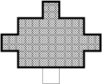
(j)

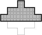
(k)

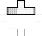
(l)

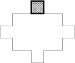
(m)

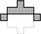
(n)

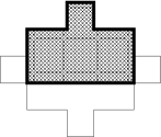
Figure 2: Illustration of the structure of the spin algebra ${A\equiv\Lambda(\bar{S}^{*})\otimes\Lambda(S^{*})}$ and the natural group action of ${\mathcal{G}\rtimes\{I,\,\overline{(\cdot)}\}}$ over it. Panel (a): the algebra $A$ with a fixed $\mathbb{Z}{\times}\mathbb{Z}$-grading (${\Lambda_{\bar{p}q}\equiv\mathop{\wedge}^{p}\bar{S}^{*}\otimes\mathop{\wedge}^{q}S^{*}}$). Panel (b): whenever a fixed $\mathbb{Z}{\times}\mathbb{Z}$-grading is taken, an element $\Psi$ of $A$ can be represented by a tuple of spinors. Panel (c): heuristically speaking, the algebra $A$ can be considered as a creation operator algebra of two distinct kind of fermions with 2 fundamental degrees of freedom each, and the two kinds being charge conjugate to each-other. Panels (d)–(e)–(f): important subspaces of the algebra $A$, namely the scalar sector $B(A)$, the maximal ideal $M(A)$, moreover the center $Z(A)$. Panels (g)–(h): illustration of the group action of the grading preserving part and of the grading non-preserving part of the symmetry group ${\mathcal{G}\rtimes\{I,\,\overline{(\cdot)}\}}$. Panels (i)–(n): list of all the subspaces of $A$, which are invariant under the group action of the symmetry group ${\mathcal{G}\rtimes\{I,\,\overline{(\cdot)}\}}$. It is seen that no invariant complementing subspaces exist, i.e. $A$ is an indecomposable multiplet.

Before we continue, we briefly mention the heuristic meaning of the representation space $A$ and the group action of $\mathcal{G}$ on it. Since ${A=\bar{\mathcal{A}}\otimes\mathcal{A}}$, the algebra $A$ can be thought of as a creation operator algebra of two kinds of fermions, each having 2 fundamental degrees of freedom, and the two kinds being related to each-other via the charge conjugation operation $\overline{(\cdot)}$. The finite dimensional real Lie group $\mathcal{G}$ acts naturally on $A$, and the meaning of grading preserving transformations of $\mathcal{G}$ is clear: they induce $\mathfrak{gl}(2,\mathbb{C})\equiv{\mathfrak{u}(1){\oplus}\,\boldsymbol{\mathtt{d}}(1){\oplus}\,\mathfrak{sl}(2,\mathbb{C})}$ transformations on the generating sector $\Lambda_{\bar{0}1}$ and corresponding natural action on all of the sectors $\Lambda_{\bar{p}q}$, and thus on the entire ${A\equiv\mathop{\bigoplus}_{p,q=0}^{2}\Lambda_{\bar{p}q}}$. The grading non-preserving transformations, isomorphic to $\mathrm{H}_{3}(\mathbb{C})$, mix higher forms to lower forms, deforming the original $\mathbb{Z}{\times}\mathbb{Z}$-grading of $A$ to an other equivalent one. In the heuristic picture of creation operator algebras, the corresponding $\mathrm{H}_{3}(\mathbb{C})$ action on an element ${\Psi\in A}$ would mean left insertion of equal amount of particles and corresponding charge conjugate particles into $\Psi$. (The spin algebra $A$ is not a CAR algebra, but is a related concept.)

In the following part we investigate important $\mathcal{G}$-invariant functions on $A$, which will be used to construct the invariant Lagrangian.

4.1 Important invariant functions on representations of the example group

In order to study the $\mathcal{G}$-invariant functions on $A$, it is convenient to first study the invariants of important “special” subgroup of it, in which the projective scaling group $\mathbb{C}^{{}^{\times}}$ is omitted, and that shall be denoted by $\mathcal{G}_{s}$. By construction, the special subgroup $\mathcal{G}_{s}$ may not only act on the full representation space ${A=\bar{\mathcal{A}}{\otimes}\mathcal{A}}$, but also on its individual factors $\mathcal{A}$ and $\bar{\mathcal{A}}$ alone. It is a further convenience to introduce some even smaller special subgroups within $\mathcal{G}_{s}$: the subgroups $S\mathcal{G}_{s}$ and $S^{{}^{\times}}\!\!\mathcal{G}_{s}$ in which the $\mathrm{D}(1)$ and the ${\mathrm{D}(1){\times}\mathrm{U}(1)}$ component is omitted, respecively. These special subgroups within $\mathcal{G}$ are most concisely presented in terms of the Lie algebra structure:

$$\mathfrak{g} \;\;\equiv\;\; \underbrace{\mathbb{C}\;\oplus\;\Big{(}\underbrace{\underbrace{\underbrace{\mathfrak{h}_{3}(\mathbb{C})\mathbin{\hbox to0.0pt{$\Leftcircle$\hss}{+}}\big{(}\mathfrak{sl}(2,\mathbb{C})}_{\text{Lie algebra of }S^{{}^{\times}}\!\!\mathcal{G}_{s}}{\oplus}\,\mathfrak{u}(1)}_{\text{Lie algebra of }S\mathcal{G}_{s}}{\oplus}\,\boldsymbol{\mathtt{d}}(1)\big{)}}_{\text{Lie algebra of }\mathcal{G}_{s}}\Big{)}}_{\text{Lie algebra of }\mathcal{G}}.\quad$$ (41)

(The subgroup ${S\mathcal{G}_{s}\subset\mathcal{G}_{s}}$ is defined by acting trivially on $M^{4}(A)$, whereas ${S^{{}^{\times}}\!\!\mathcal{G}_{s}\subset S\mathcal{G}_{s}}$ is defined by acting trivially also on $M^{2}(\mathcal{A})$.) Our strategy will be to first find invariants of the representations of the special subgroups ${S^{{}^{\times}}\!\!\mathcal{G}_{s}}$ on $\mathcal{A}$ and of ${S\mathcal{G}_{s}}$ on $A$. Then, we will study the action of the dilatation $\mathrm{D}(1)$ group and the projective scaling group $\mathbb{C}^{{}^{\times}}$ on the ensemble of the found invariants, in order to construct invariants of the full group $\mathcal{G}$.

Using the LieAlgebras Maple package Anderson2016 , one can search for invariant functions of the pertinent special groups. For instance, one can show that there is a single functionally independent ${\mathcal{A}\rightarrow\mathbb{C}}$ map, which is invariant to the group action of $S^{{}^{\times}}\!\!\mathcal{G}_{s}$, and is nothing but the scalar component function ${b:\mathcal{A}\rightarrow\mathbb{C},\psi\mapsto b\psi}$, where $b$ picks out the scalar component (bottom-form or zero-form) of an element of $\mathcal{A}$. In a two-spinor representation ${\psi\equiv(\phi,\,\xi_{{}_{A}},\,\varepsilon_{{}_{BC}})}$ of an element ${\psi\in\mathcal{A}}$, one has that ${b\psi=\phi}$. Similarly, one can search for ${\mathcal{A}\times\mathcal{A}\rightarrow\mathbb{C}}$ functions, invariant to $S^{{}^{\times}}\!\!\mathcal{G}_{s}$, and these turn out to be functional combinations of these three invariants:

$$(\psi,\psi^{\prime}) \mapsto b\psi,$$ (42)

$$(\psi,\psi^{\prime}) \mapsto b\psi^{\prime},$$ (43)

$$(\psi,\psi^{\prime}) \mapsto \lambda(\psi_{,}\psi^{\prime}):=(b\partial_{1}\psi)(b\partial_{2}\psi^{\prime})-(b\partial_{2}\psi)(b\partial_{1}\psi^{\prime})-(b\psi)(b\partial_{2}\partial_{1}\psi^{\prime})+(b\partial_{2}\partial_{1}\psi)(b\psi^{\prime})$$ (44)

where ${\partial_{1},\partial_{2}}$ denote stepping down operators associated to some arbitrarily chosen generators ${a_{1},a_{2}\in\Lambda_{1}}$. In two-spinor representation by setting ${\psi\equiv(\phi,\,\xi_{{}_{A}},\,\varepsilon_{{}_{BC}})}$ and ${\psi^{\prime}\equiv(\phi^{\prime},\,\xi^{\prime}_{{}_{A}},\,\varepsilon^{\prime}_{{}_{BC}})}$ one has that

$$\lambda(\psi,\psi^{\prime})=\tfrac{1}{2}\boldsymbol{\epsilon}^{{}_{AB}}\left(\xi{}_{{}_{A}}\xi^{\prime}{}_{{}_{B}}-\xi^{\prime}{}_{{}_{A}}\xi{}_{{}_{B}}+\phi\,\varepsilon^{\prime}{}_{{}_{AB}}-\phi^{\prime}\,\varepsilon{}_{{}_{AB}}\right),$$ (46)

where ${\boldsymbol{\epsilon}_{{}_{AB}}\in\mathop{\wedge}^{2}S^{*}\equiv M^{2}(\mathcal{A})}$ is an arbitrary but fixed nonzero maximal form in $\mathcal{A}$, and $\boldsymbol{\epsilon}^{{}_{AB}}$ is its corresponding inverse maximal form satisfying ${\boldsymbol{\epsilon}_{{}_{AB}}\,\boldsymbol{\epsilon}^{{}_{CB}}=\delta_{{}_{A}}{}^{{}_{C}}}$. It is seen that $\lambda$ is a nondegenerate symplectic form, and that its choice is unique up to a complex multiplier, i.e. up to the choice of $\boldsymbol{\epsilon}_{{}_{AB}}$. One could say that the symplectic form $\lambda$ is a generalization of the symplectic form $\boldsymbol{\epsilon}^{{}_{AB}}$ from two-spinors to their exterior algebra. It is seen that $\lambda$ is uniquely determined up to complex normalization, where the ambiguity comes from the choice of the nonzero maximal form ${\boldsymbol{\epsilon}_{{}_{AB}}\in M^{2}(\mathcal{A})}$. In order to fix this normalization ambiguity in the formalism, one could consider instead the “densitized version” of $\lambda$. That can be defined to be the unique $\mathcal{G}_{s}$-invariant symplectic form ${\boldsymbol{\lambda}:\,\mathcal{A}\times\mathcal{A}\rightarrow M^{2}(\mathcal{A})}$ satisfying the natural normalization condition ${\boldsymbol{\lambda}(\mathds{1},\boldsymbol{\epsilon})=\boldsymbol{\epsilon}}$ for all maximal forms ${\boldsymbol{\epsilon}\in M^{2}(\mathcal{A})}$.

Using again the LieAlgebras Maple package Anderson2016 , one can search for $S\mathcal{G}_{s}$-invariant functions of $A$. For instance, one can show that there is a single functionally independent invariant ${A\rightarrow\mathbb{C}}$ function, namely ${\bar{b}{\otimes}b}$, picking out the scalar component (bottom-form or zero-form) of an element in $A$. In the following we shall use the abbreviation $b$ for ${\bar{b}{\otimes}b}$, since their distinction is not relevant. Similarly, one can search for ${A\times A\rightarrow\mathbb{C}}$ functions, invariant to $S\mathcal{G}_{s}$, and these turn out to be functional combinations of these three invariants:

$$(\Psi,\Psi^{\prime}) \mapsto b\Psi,$$ (47)

$$(\Psi,\Psi^{\prime}) \mapsto b\Psi^{\prime},$$ (48)

$$(\Psi,\Psi^{\prime}) \mapsto L(\Psi_{,}\Psi^{\prime}):=\left(\bar{\lambda}{\otimes}\lambda\right)\circ\left(I_{\bar{\mathcal{A}}}{\otimes}J{\otimes}I_{\mathcal{A}}\right)(\Psi\otimes\Psi^{\prime})$$ (49)

where $J$ denotes the ${\mathcal{A}\otimes\bar{\mathcal{A}}\rightarrow\bar{\mathcal{A}}\otimes\mathcal{A}}$ swapping map, whereas $I_{\bar{\mathcal{A}}}$ and $I_{\mathcal{A}}$ denote the identity map of $\bar{\mathcal{A}}$ and $\mathcal{A}$, respectively. If a preferred $\mathbb{Z}{\times}\mathbb{Z}$-grading is taken along with generators ${a_{1},a_{2}\in\Lambda_{\bar{0}1}}$, and corresponding stepping down operators ${\partial_{1},\partial_{2}}$, then the concrete expression

$$L(\Psi,\Psi^{\prime}) = b\bar{\partial}_{2}\bar{\partial}_{1}\partial_{2}\partial_{1}\big{(}(\Psi_{\bar{0}0}-\Psi_{\bar{1}0}-\Psi_{\bar{0}1}+\Psi_{\bar{1}1}-\Psi_{\bar{2}0}-\Psi_{\bar{0}2}+\Psi_{\bar{2}1}+\Psi_{\bar{1}2}+\Psi_{\bar{2}2})\,\Psi^{\prime}\big{)}\Big{.}\qquad$$ (50)

holds for all ${\Psi,\Psi^{\prime}\in A}$. By construction, $L$ is a nondegenerate symmetric bilinear form with alternating signature (${{+}1,{-}1,{+}1,{-}1,\dots}$). When expressed in terms of two-spinor representation ${A\equiv\Lambda(\bar{S}^{*})\otimes\Lambda(S^{*})}$, then for two elements

$$\begin{array}[]{l}\Psi\equiv\Big{(}\phi,\,\bar{\xi}_{{}_{(+)A^{\prime}}},\,\xi_{{}_{(-)A}},\,\bar{\varepsilon}_{{}_{(+)A^{\prime}B^{\prime}}},\,v{}_{{}_{A^{\prime}B}},\,\varepsilon_{{}_{(-)AB}},\,\bar{\chi}_{{}_{(+)A^{\prime}B^{\prime}C}},\,\chi_{{}_{(-)C^{\prime}AB}},\,\omega_{{}_{A^{\prime}B^{\prime}AB}}\Big{)}\cr\end{array}$$

and

$$\begin{array}[]{l}\Psi^{\prime}\equiv\Big{(}\phi^{\prime},\,\bar{\xi}^{\prime}_{{}_{(+)A^{\prime}}},\,\xi^{\prime}_{{}_{(-)A}},\,\bar{\varepsilon}^{\prime}_{{}_{(+)A^{\prime}B^{\prime}}},\,v^{\prime}{}_{{}_{A^{\prime}B}},\,\varepsilon^{\prime}_{{}_{(-)AB}},\,\bar{\chi}^{\prime}_{{}_{(+)A^{\prime}B^{\prime}C}},\,\chi^{\prime}_{{}_{(-)C^{\prime}AB}},\,\omega^{\prime}_{{}_{A^{\prime}B^{\prime}AB}}\Big{)}\cr\end{array}$$

one has the identity

$$L(\Psi,\Psi^{\prime})=\tfrac{1}{4}\boldsymbol{\omega}^{{}_{A^{\prime}B^{\prime}CD}}\Big{(}$$ (51)

$$\Big{.}\phi\,\omega^{\prime}_{{}_{A^{\prime}B^{\prime}CD}}+\omega_{{}_{A^{\prime}B^{\prime}CD}}\,\phi^{\prime}+4v_{{}_{A^{\prime}C}}\,v^{\prime}_{{}_{B^{\prime}D}}-\bar{\varepsilon}_{{}_{(+)A^{\prime}B^{\prime}}}\,\varepsilon^{\prime}_{{}_{(-)CD}}-\varepsilon_{{}_{(-)CD}}\,\bar{\varepsilon}^{\prime}_{{}_{(+)A^{\prime}B^{\prime}}}$$ (52)

$$-2\bar{\xi}_{{}_{(+)A^{\prime}}}\,\chi^{\prime}_{{}_{(-)B^{\prime}CD}}-2\xi_{{}_{(-)C}}\,\bar{\chi}^{\prime}_{{}_{(+)A^{\prime}B^{\prime}D}}+2\bar{\chi}_{{}_{(+)A^{\prime}B^{\prime}C}}\,\xi^{\prime}_{{}_{(-)D}}+2\chi_{{}_{(-)A^{\prime}CD}}\,\bar{\xi}^{\prime}_{{}_{(+)B^{\prime}}}\Big{)},$$ (53)

where ${\boldsymbol{\omega}_{{}_{A^{\prime}B^{\prime}CD}}\in\mathop{\wedge}^{2}\bar{S}^{*}\otimes\mathop{\wedge}^{2}S^{*}\equiv M^{4}(A)}$ is an arbitrary but fixed nonzero positive maximal form of $A$, and $\boldsymbol{\omega}^{{}_{A^{\prime}B^{\prime}CD}}$ is its inverse maximal form with the normalization convention ${\boldsymbol{\omega}_{{}_{A^{\prime}B^{\prime}DE}}\;\boldsymbol{\omega}^{{}_{C^{\prime}B^{\prime}FE}}=\bar{\delta}_{{}_{A^{\prime}}}{}^{{}_{C^{\prime}}}\,\delta_{{}_{D}}{}^{{}_{F}}}$. The invariant bilinear form $L$ shall be shown to be a kind of generalization of the form related to the Dirac adjoint, and will be a key object in defining $\mathcal{G}$-invariant Lagrangians. It is seen that $L$ is uniquely determined up to complex normalization, where the ambiguity comes from the choice of the nonzero maximal form ${\boldsymbol{\omega}_{{}_{A^{\prime}B^{\prime}CD}}\in M^{4}(A)}$. In order to fix this normalization ambiguity in the formalism, one could consider instead the “densitized version” of $L$. That can be defined to be the unique $\mathcal{G}_{s}$-invariant symmetric bilinear form ${\mathbf{L}:\,A\times A\rightarrow M^{4}(A)}$ with the natural normalization condition ${\mathbf{L}(\mathds{1},\boldsymbol{\omega})=\boldsymbol{\omega}}$ for all maximal forms ${\boldsymbol{\omega}\in M^{4}(A)}$.

Before we can go on to the formulation of $\mathcal{G}$-invariant theories, invocation of some further invariant objects is necessary, related to the two-spinor calculus. As it is well known PR1984 ; Wald1984 , in the ordinary two-spinor formalism the spinor space $S$ is considered as a representation space of $\mathrm{GL}(S)$, and by requiring the invariance of the duality pairing form and of the complex conjugation map, a canonical representation of $\mathrm{GL}(S)$ is defined also on $S^{*}$, $\bar{S}$, $\bar{S}^{*}$, respectively. Therefore, one has a canonical representation on the tensor product space ${\bar{S}{\otimes}S}$, as well as on its real part ${\mathop{\mathrm{Re}}\nolimits}\big{(}\bar{S}{\otimes}S\big{)}$. The formalism of two-spinor calculus is based on the fact that on the four dimensional real vector space ${\mathop{\mathrm{Re}}\nolimits}\big{(}\bar{S}{\otimes}S\big{)}$ the canonical representation of $\mathrm{GL}(S)$ reduces to a representation of the Weyl group (dilatation + Lorentz group). More concretely, for any nonzero maximal form ${\boldsymbol{\epsilon}_{{}_{AB}}\in\mathop{\wedge}^{2}S^{*}}$ one has that the form ${\boldsymbol{\omega}_{{}_{A^{\prime}B^{\prime}AB}}:=\bar{\boldsymbol{\epsilon}}_{{}_{A^{\prime}B^{\prime}}}\otimes\boldsymbol{\epsilon}_{{}_{AB}}}$ defines a nondegenerate, symmetric, Lorentz signature (+,-,-,-) real-bilinear form on ${{\mathop{\mathrm{Re}}\nolimits}\big{(}\bar{S}{\otimes}S\big{)}}$, which is preserved by the action of $\mathrm{GL}(S)$ up to positive multiplier. Therefore, if some other four dimensional real vector space $T$ is taken (which one may call “tangent space”), and a linear injection ${\sigma_{a}^{{}_{A^{\prime}A}}:T\rightarrow{\mathop{\mathrm{Re}}\nolimits}\big{(}\bar{S}{\otimes}S\big{)}}$ is fixed, then the $\mathrm{GL}(S)$-induced Weyl group representation is pulled back onto $T$, via requiring the $\sigma_{a}^{{}_{A^{\prime}A}}$ to be invariant MR96276 . By construction, this representation of $\mathrm{GL}(S)$ respects the Lorentz metric ${g(\sigma,\boldsymbol{\omega})_{ab}:=\sigma_{a}^{{}_{A^{\prime}A}}\,\sigma_{b}^{{}_{B^{\prime}B}}\,\boldsymbol{\omega}_{{}_{A^{\prime}B^{\prime}AB}}}$ on $T$ up to positive multiplier. The map $\sigma_{a}^{{}_{A^{\prime}A}}$ is called soldering form or Pauli map or Infeld–Van der Waerden symbol in the literature. The pertinent philosophy naturally generalizes to the spin algebra case: the subspaces ${M(\mathcal{A})\subset\mathcal{A}}$ and ${M^{2}(\mathcal{A})\subset M(\mathcal{A})}$ are invariant under the canonical representation of $\mathcal{G}_{s}$ on $\mathcal{A}$, and therefore one has the natural $\mathcal{G}_{s}$-invariant induced representation on the quotient space ${S^{*}\equiv M(\mathcal{A})/M^{2}(\mathcal{A})}$, and on its dual ${S\equiv\big{(}M(\mathcal{A})/M^{2}(\mathcal{A})\big{)}^{*}}$. Because of that, one can take a real-linear injection ${\sigma_{a}^{{}_{A^{\prime}A}}:T\rightarrow{\mathop{\mathrm{Re}}\nolimits}\big{(}\bar{S}\otimes S\big{)}}$ into the $\mathcal{G}_{s}$-invariant space ${\mathop{\mathrm{Re}}\nolimits\big{(}\bar{S}\otimes S\big{)}}$. Clearly, fixing such a soldering form $\sigma_{a}^{{}_{A^{\prime}A}}$ pulls back the natural real-linear representation of the group $\mathcal{G}_{s}$ onto $T$, via the requirement of the soldering form $\sigma_{a}^{{}_{A^{\prime}A}}$ to be invariant. Similarly to the ordinary two-spinor case, this induced linear representation of $\mathcal{G}_{s}$ on $T$ is nothing but the Weyl group: the Lorentz group together with the metric rescalings.

It is sometimes useful to construct a further equivalent realization of the soldering form, in the spin algebra context. Using the LieAlgebras Maple package Anderson2016 , one can show that the subspace of elements of $\mathop{\mathrm{Lin}}\nolimits(\mathcal{A})$ which are invariant to the Heisenberg (nilpotent) group action of ${\exp L_{M(\mathcal{A})}}$, is nothing but $R_{\mathcal{A}}$, i.e. the image of $\mathcal{A}$ in $\mathop{\mathrm{Lin}}\nolimits(\mathcal{A})$ by the right multiplication. Correspondingly, the Heisenberg-invariant elements in $\mathop{\mathrm{Lin}}\nolimits(\bar{\mathcal{A}})$ span $R_{\bar{\mathcal{A}}}$. Therefore, one has the natural $\mathcal{G}_{s}$-invariant injections by right multiplication

$$S^{*}\rightarrow R_{\mathcal{A}} \;,\quad \xi_{{}_{B}}\mapsto\xi_{{}_{B}}R_{\boldsymbol{\delta}^{B}}$$ (54)

$$\Big{.}\bar{S}^{*}\rightarrow R_{\bar{\mathcal{A}}} \;,\quad \bar{\xi}_{{}_{B^{\prime}}}\mapsto\bar{\xi}_{{}_{B^{\prime}}}R_{\bar{\boldsymbol{\delta}}^{B^{\prime}}}$$ (55)

of the co-spinor spaces into the space right multiplication operators ${R_{\mathcal{A}}\subset\mathop{\mathrm{Lin}}\nolimits(\mathcal{A})}$ and ${R_{\bar{\mathcal{A}}}\subset\mathop{\mathrm{Lin}}\nolimits(\bar{\mathcal{A}})}$, respectively. We used Penrose indices on spinor side, and suppressed indices on the algebra side in order to introduce the right injection operators $R_{\boldsymbol{\delta}^{B}}$ and $R_{\bar{\boldsymbol{\delta}}^{B^{\prime}}}$. Analoguously, using the LieAlgebras Maple package Anderson2016 , one can show that the subspace of elements of $\mathop{\mathrm{Lin}}\nolimits(A)$ which are Heisenberg-invariant is $R_{A}$. After verifying these facts, it follows that, up to a real multiplier, the only $\mathcal{G}_{s}$-invariant ${T^{*}\rightarrow\mathop{\mathrm{Lin}}\nolimits(A)}$ real-linear injective map is $\boldsymbol{\sigma}^{b}:=\sigma^{b}_{{}^{B^{\prime}B}}\,R_{\bar{\boldsymbol{\delta}}^{B^{\prime}}}{\otimes}R_{\boldsymbol{\delta}^{B}}$, where ${\sigma^{b}_{{}^{B^{\prime}B}}:{\mathop{\mathrm{Re}}\nolimits}(\bar{S}{\otimes}S)\rightarrow T}$ is the usual two-spinorial inverse soldering form, uniquely determined via the relation ${\sigma^{b}_{{}^{B^{\prime}B}}\,\sigma_{a}^{{}_{B^{\prime}B}}=\delta^{b}{}_{a}}$. The normalization of $\boldsymbol{\sigma}^{b}$ and $\sigma_{a}^{{}_{A^{\prime}A}}$ can be uniquely interlinked via fixing the natural normalization identity ${\big{(}(\boldsymbol{\sigma}^{b}\mathds{1})\big{/}M^{3}(A)\big{)}_{{}^{B^{\prime}B}}\,\sigma_{a}^{{}_{B^{\prime}B}}=\delta^{b}{}_{a}}$.

Given a fixed soldering form $\sigma_{a}^{{}_{A^{\prime}A}}$ and a fixed real maximal form ${\boldsymbol{\omega}\in\mathop{\mathrm{Re}}\nolimits(M^{4}(A))}$, the previously introduced Lorentz metric ${g(\sigma,\boldsymbol{\omega})_{ab}}$ is a naturally defined $S\mathcal{G}_{s}$-invariant object. The normalization of the metric $g(\sigma,\boldsymbol{\omega})_{ab}$ is, however, ambiguous up to the choice of $\boldsymbol{\omega}$. In order to fix this normalization ambiguity in the formalism, one could consider instead the “densitized version” of the metric. That can be defined to be the unique $\mathcal{G}_{s}$-invariant symmetric bilinear form ${\mathbf{g}(\sigma)_{ab}:\,T\times T\rightarrow\mathop{\mathrm{Re}}\nolimits(M^{4}(A))^{*}}$, satisfying ${(u^{a}\,v^{b}\,\mathbf{g}(\sigma)_{ab}\,|\,\boldsymbol{\omega})=u^{a}\,v^{b}\,g(\sigma,\boldsymbol{\omega})_{ab}}$ for all ${\boldsymbol{\omega}\in\mathop{\mathrm{Re}}\nolimits(M^{4}(A))}$ and ${u^{a},v^{a}\in T}$. The corresponding densitized inverse metric, being a symmetric bilinear form ${\mathbf{g}(\sigma)^{ab}:\,T^{*}\times T^{*}\rightarrow\mathop{\mathrm{Re}}\nolimits(M^{4}(A))}$, is uniquely determined by the relation ${\mathbf{g}(\sigma)_{ab}\,\mathbf{g}(\sigma)^{bc}=\delta^{c}{}_{a}}$. The densitized inverse metric can also be expressed in terms of the ordinary, real valued inverse metric via the identity ${\mathbf{g}(\sigma)^{ab}=\boldsymbol{\omega}\,g(\sigma,\boldsymbol{\omega})^{ab}}$, given any nonvanishing ${\boldsymbol{\omega}\in\mathop{\mathrm{Re}}\nolimits(M^{4}(A))}$. Associated to the metric $g(\sigma,\boldsymbol{\omega})_{ab}$, also a unique volume form in ${\mathop{\wedge}^{4}T^{*}}$ exists (up to orientation), and that is known to be expressable in the form

$$\begin{array}[]{l}\mathrm{v}(o,\sigma,\boldsymbol{\omega})_{abcd}\;:=\cr\qquad\Big{.}o\;\big{(}\,\mathrm{i}\,\sigma_{a}^{{}^{{}_{E^{\prime}E}}}\,\sigma_{b}^{{}^{{}_{F^{\prime}F}}}\,\sigma_{c}^{{}^{{}_{B^{\prime}A}}}\,\sigma_{d}^{{}^{{}_{A^{\prime}B}}}\,\boldsymbol{\omega}_{{}_{E^{\prime}A^{\prime}EA}}\,\boldsymbol{\omega}_{{}_{F^{\prime}B^{\prime}FB}}-\mathrm{i}\,\sigma_{a}^{{}^{{}_{E^{\prime}E}}}\,\sigma_{b}^{{}^{{}_{F^{\prime}F}}}\,\sigma_{d}^{{}^{{}_{B^{\prime}A}}}\,\sigma_{c}^{{}^{{}_{A^{\prime}B}}}\,\boldsymbol{\omega}_{{}_{E^{\prime}A^{\prime}EA}}\,\boldsymbol{\omega}_{{}_{F^{\prime}B^{\prime}FB}}\,\big{)}\cr\end{array}$$

PR1984 ; Wald1984 , where ${o=\pm 1}$ describes the chosen orientation sign. The normalization of the volume form also depends on the choice of an ${\boldsymbol{\omega}\in\mathop{\mathrm{Re}}\nolimits(M^{4}(A))}$. In order to fix this normalization ambiguity, the corresponding densitized volume form is introduced, which is the unique element ${\mathbf{v}(o,\sigma)\in\mathop{\wedge}^{4}T^{*}\,\otimes\,\mathop{\mathrm{Re}}\nolimits(M^{4}(A))^{*}\otimes\mathop{\mathrm{Re}}\nolimits(M^{4}(A))^{*}}$ satisfying ${(\mathbf{v}(o,\sigma)\,|\,\boldsymbol{\omega}{\otimes}\,\boldsymbol{\omega})=\mathrm{v}(o,\sigma,\boldsymbol{\omega})}$ for all ${\boldsymbol{\omega}\in\mathop{\mathrm{Re}}\nolimits(M^{4}(A))}$. By construction, the densitized volume form $\mathbf{v}(o,\sigma)$ is also $\mathcal{G}_{s}$-invariant.

The spin tensor is a further invariant function of $\sigma_{a}^{{}_{A^{\prime}A}}$ according to the definition

$$\Sigma(\sigma){}_{a}{}^{b}{}_{{}_{C}}{}^{{}_{D}}:=\mathrm{i}\,\sigma_{a}^{{}_{A^{\prime}D}}\,\sigma^{b}_{{}^{A^{\prime}C}}-\mathrm{i}\,\mathbf{g}(\sigma)^{cb}\,\mathbf{g}(\sigma)_{ad}\,\sigma_{c}^{{}_{A^{\prime}D}}\,\sigma^{d}_{{}^{A^{\prime}C}}$$

which is a tensor of ${T^{*}{\otimes}T\otimes S^{*}{\otimes}}S$, using the identification ${S^{*}\equiv M(\mathcal{A})\big{/}M^{2}(\mathcal{A})}$ as previously. The spin tensor $\Sigma(\sigma){}_{a}{}^{b}{}_{{}_{C}}{}^{{}_{D}}$, by construction, is also $\mathcal{G}_{s}$-invariant.

The introduced formalism is all as usual in the ordinary two-spinor calculus PR1984 ; Wald1984 , with the slight generalization of providing some extra representation space ${\mathcal{A}\equiv\Lambda(S^{*})}$ for the nilpotent Lie group component $\mathrm{H}_{3}(\mathbb{C})$ of our symmetry group $\mathcal{G}$, where $\mathcal{G}$ as acting on $A$ can be considered as a generalization of $\mathrm{GL}(S^{*})$ as acting on $S^{*}$.

5 The example Lagrangian

In order to define our Lagrangian, we assume that our matter fields are sections of an $A$-valued vector bundle over a four dimensional spacetime, as illustrated in Figure 3. A distantly similar construction was considered by Anco and Wald Anco1989 , but the algebra they employed was too small in order to accommodate representation space for any symmetries larger than the conventional direct product symmetries, based merely on reductive Lie algebras.

In our construction, we consider a four dimensional real manifold $\mathcal{M}$ (which we shall call the spacetime manifold), and a vector bundle over $\mathcal{M}$ with fiber $A$ and structure group $\mathcal{G}$, as defined in Eq.(37). As we shall see, such a structure exists whenever $\mathcal{M}$ is spin. The bundle $A(\mathcal{M})$ is a spin algebra valued vector bundle of the form ${A(\mathcal{M})=\bar{\mathcal{A}}(\mathcal{M}){\otimes}\mathcal{A}(\mathcal{M})}$ with $\mathcal{A}(\mathcal{M})$ being a two generator complex Grassmann algebra bundle over $\mathcal{M}$. Analogously to ordinary two-spinor calculus PR1984 ; Wald1984 , we assume a $\sigma_{a}^{{}_{A^{\prime}A}}$ pointwise injective ${T(\mathcal{M})\rightarrow\mathop{\mathrm{Re}}\nolimits\big{(}\bar{S}(\mathcal{M}){\otimes}\,S(\mathcal{M})\big{)}}$ vector bundle morphism (soldering form) to be present, where ${S^{*}(\mathcal{M}):=M(\mathcal{A})(\mathcal{M})\big{/}M^{2}(\mathcal{A})(\mathcal{M})}$ plays the role of an ordinary lower index two-spinor bundle. We see from the above that given a spacetime $\mathcal{M}$ with co-spinor bundle $S^{*}(\mathcal{M})$, and a choice of soldering form $\sigma_{a}^{{}_{A^{\prime}A}}$, we can construct a spin algebra valued bundle $A(\mathcal{M})$ over $\mathcal{M}$. The charge conjugation group ${\{I,\,\overline{(\cdot)}\}\equiv\mathbb{Z}_{2}}$, which has a canonical action on the sections of $A(\mathcal{M})$, will be required to be a global symmetry of the model.

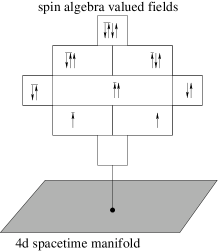
Figure 3: Illustration of the concept of spin algebra valued fields. The structure group of such a theory can be set to be a conservative unification $\mathcal{G}$ of the Lorentz (or Weyl) and of the compact $\mathrm{U}(1)$ symmetries.

Let $\nabla_{a}$ be a covariant derivation operator on $A(\mathcal{M})$. In the model, these will play the role of mediator fields. The adjoining by the discrete group of charge conjugation ${\{I,\,\overline{(\cdot)}\}\equiv\mathbb{Z}_{2}}$ acts trivially on ${\mathcal{G}_{s}\subset\mathcal{G}}$, but acts nontrivially on the projective scaling subgroup ${\mathbb{C}^{{}^{\times}}\subset\mathcal{G}}$. Therefore, the charge conjugation map takes a covariant derivation $\nabla_{a}$ in general to a different covariant derivation $\overline{\nabla}_{a}$, according to the canonical action ${\overline{\nabla}_{a}\Psi:=\overline{\nabla_{a}\overline{\Psi}}}$, for any section $\Psi$ of $A(\mathcal{M})$. It is straightforward to check that the differential operator ${\nabla_{a}^{\mathbb{R}}:=\tfrac{1}{2}\big{(}\nabla_{a}+\overline{\nabla}_{a}\big{)}}$ also defines a covariant derivation. By construction, the charge conjugation $\overline{(\cdot)}$ acts trivially on $\nabla_{a}^{\mathbb{R}}$. Since on $\mathcal{G}_{s}$ the adjoining by charge conjugation acts trivially, and also on the subgroup $|\mathbb{C}^{{}^{\times}}|$ of the projective scaling group $\mathbb{C}^{{}^{\times}}$, one has the gauge potential ${\nabla_{a}{-}\nabla_{a}^{\mathbb{R}}}$ is simply a covector field carrying gauge charge of merely the quotient ${\mathbb{C}^{{}^{\times}}/|\mathbb{C}^{{}^{\times}}|}$. Therefore, the mapping ${\nabla_{a}\mapsto\nabla_{a}^{\mathbb{R}}}$ takes a covariant derivation to an other covariant derivation, with the gauge potential corresponding to the complex phase of the projective subgroup $\mathbb{C}^{{}^{\times}}$ zeroed. This slight complication with the distinction between $\nabla_{a}$ and $\nabla_{a}^{\mathbb{R}}$ in the formalism comes from the convention that we would like to handle projective representations of $\mathcal{G}_{s}$ via addressing linear representations of $\mathcal{G}$, and it does not have any particular physics meaning or relevance. The physically relevant part of $\nabla_{a}$ will turn out to be simply $\nabla_{a}^{\mathbb{R}}$ in the model.

Our action principle shall be Palatini-like, i.e. the metric will not be a distinguished field. In fact, it will be a function of an other fundamental field: the soldering form $\sigma_{a}^{{}_{A^{\prime}A}}$. The matter field sector of the theory will consist of the soldering form $\sigma_{a}^{{}_{A^{\prime}A}}$ and of a section $\Psi$ of the spin algebra bundle $A(\mathcal{M})$. Moreover, as in the Palatini formalism, the covariant derivation $\nabla_{a}$ is independently varied from the matter field sector. That is, $\nabla_{a}$ physically describes a combined gravitational-and-gauge connection, without an a priori splitting into a gravitational and an internal part. In total, the independent field variables form a tuple ${\big{(}\sigma_{a}^{{}_{A^{\prime}A}},\,\Psi,\,\nabla_{b}\big{)}}$. The subgroup $\mathcal{G}_{s}$ of the structure group $\mathcal{G}$ has a canonical action on these, introduced in the previous sections. The charge conjugation group ${\{I,\,\overline{(\cdot)}\}\equiv\mathbb{Z}_{2}}$ as a global symmetry group also has a natural action via representing the charge conjugation map as ${\big{(}\sigma_{a}^{{}_{A^{\prime}A}},\,\Psi,\,\nabla_{b}\big{)}\,\mapsto\,\big{(}{-}\sigma_{a}^{{}_{A^{\prime}A}},\,\overline{\Psi},\,\overline{\nabla}_{b}\big{)}}$ on the fields, which can be understood as the action of a local $CPT$ transformation. (The field $\Psi$ is charge conjugated, and simultaneously, the sign of the soldering $\sigma_{a}^{{}_{A^{\prime}A}}$ of the spin algebra to the spacetime vectors is reversed.) The projective scaling subgroup $\mathbb{C}^{{}^{\times}}$ of $\mathcal{G}$ is defined to act on the fields as ${\big{(}\sigma_{a}^{{}_{A^{\prime}A}},\,\Psi,\,\nabla_{b}\big{)}\,\mapsto\,\big{(}|z|\,\sigma_{a}^{{}_{A^{\prime}A}},\,z\,\Psi,\,z\nabla_{b}z^{-1}\big{)}}$ for a projective scaling field $z$, being a section of the ${\mathbb{C}^{{}^{\times}}}$ valued line bundle. Thus at this point, the action of the structure group $\mathcal{G}$ and the global charge conjugation group ${\{I,\,\overline{(\cdot)}\}\equiv\mathbb{Z}_{2}}$ on the fields ${\big{(}\sigma_{a}^{{}_{A^{\prime}A}},\,\Psi,\,\nabla_{b}\big{)}}$ is fully specified.

The actual Lagrangian shall be a real volume form valued pointwise vector bundle mapping

$$\begin{array}[]{l}(o,\,\sigma_{a}^{{}_{A^{\prime}A}},\,\Psi,\,\nabla_{a}\Psi,\,P(\nabla)_{ab})\;\longmapsto\;\mathrm{L}(o,\,\sigma_{a}^{{}_{A^{\prime}A}},\,\Psi,\,\nabla_{a}\Psi,\,P(\nabla)_{ab})\cr\end{array}$$ (56)

with the requirement of being invariant to the vector bundle automorphisms of $A(\mathcal{M})$ compatible with the structure group $\mathcal{G}$. The symbol $P(\nabla)_{ab}$ denotes the curvature tensor of a covariant derivation $\nabla_{a}$, and $o$ denotes the spacetime orientation sign (${o=\pm 1}$). The action functional is, as usually, defined to be local integrals of the pertinent volume form over compact regions of the spacetime $\mathcal{M}$. We also require the action functional of the theory to be invariant to the change of the spacetime orientation $o$, which implies that the Lagrangian should flip sign when changing the spacetime orientation $o$ to opposite. This explicitely forbids Chern–Simons-like terms in the model. In addition to these quite conventional gauge-theory-like symmetry prescriptions, we require the Lagrangian to be invariant to a shift transformation of the gauge-covariant derivation according to ${\nabla_{a}\mapsto\nabla_{a}+C_{a}}$ in the manner of Section 3, where $C_{a}$ denotes a smooth covector field taking its values in the ideal of $\mathcal{G}$, corresponding to the ${\mathbb{C}^{{}^{\times}}\times\big{(}\mathrm{H}_{3}(\mathbb{C})\rtimes\mathrm{D}(1)\big{)}}$ part. This requirement means that the Lagrangian should not depend on all the $\mathcal{G}$-connection fields, but only on modes with $\mathrm{U}(1)$ or $\mathrm{SL}(2,\mathbb{C})$ charges. The search for all such invariant volume form valued expressions in principle can be addressed by the LieAlgebras Maple package Anderson2016 . However, due to the relatively large dimension of the total pointwise degrees of freedom, the pertinent library was not able to answer this question in its full generality. We were able to find, though, all the invariant terms, with certain fixed polynomial degree in $P(\nabla)_{ab}$ and in $\nabla_{a}\Psi$. There is strong evidence that these are all the invariants. The pertinent invariant terms are enumerated in the following, listed according to their polynomial degree in $P(\nabla)_{ab}$ and $\nabla_{a}\Psi$.

Yang–Mills-like term. The tensor field $\mathbf{v}(o,\sigma)\,\mathbf{g}(\sigma)^{ab}\,\mathbf{g}(\sigma)^{cd}$ only depends on the orientation $o$ and the soldering form $\sigma$, and it is $\mathcal{G}$-invariant. Due to the structure of the group $\mathcal{G}$, the curvature $P(\nabla)_{ab}$ of a covariant derivation $\nabla_{a}$ does have a canonical action not only as a $\mathop{\mathrm{Lin}}\nolimits(A)$-valued two-form, but also as a $\mathop{\mathrm{Lin}}\nolimits(S^{*})$-valued two-form with the usual identification ${S^{*}\equiv M(\mathcal{A})/M^{2}(\mathcal{A})\cong\Lambda_{\bar{0}1}}$. Therefore, its restricted trace ${\left.\mathop{\mathrm{Tr}}\nolimits\right|_{\Lambda_{\bar{0}1}}P(\nabla)_{ab}}$ is meaningful, and is a $\mathcal{G}$-gauge covariant expression. With the introduced quantities, it does not come as a surprise that the only invariant Lagrangian bilinear in the curvature $P(\nabla)_{ab}$ and satisfying positive energy density condition for gauge fields is:

$$\begin{array}[]{l}\mathrm{L}_{{}_{\mathrm{YM}}}(o,\,\sigma_{a}^{{}_{A^{\prime}A}},\,\Psi,\,\nabla_{a}\Psi,\,P(\nabla)_{ab})\;:=\cr\qquad\Big{.}\mathbf{v}(o,\sigma)\,\mathbf{g}(\sigma)^{ac}\,\mathbf{g}(\sigma)^{bd}\,\mathop{\mathrm{Im}}\nolimits\big{(}\left.\mathop{\mathrm{Tr}}\nolimits\right|_{\Lambda_{\bar{0}1}}P(\nabla^{\mathbb{R}})_{ab}\big{)}\,\mathop{\mathrm{Im}}\nolimits\big{(}\left.\mathop{\mathrm{Tr}}\nolimits\right|_{\Lambda_{\bar{0}1}}P(\nabla^{\mathbb{R}})_{cd}\big{)}.\end{array}$$ (57)

This is nothing but literally the Maxwell Lagrangian, as expressed in our field variables. It is remarkable that only the $\mathrm{U}(1)$ part of the connection gives contribution, while the expression being $\mathcal{G}$-covariant.

Einstein–Hilbert-like term. The tensor field $\mathbf{v}(o,\sigma)\,\mathbf{g}(\sigma)^{ab}\,\mathbf{L}(\overline{\Psi},\Psi)$ is $\mathcal{G}$-invariant. Thus, it is not surprising that the only invariant Lagrangian linear in the curvature $P(\nabla)_{ab}$ is:

$$\begin{array}[]{l}\mathrm{L}_{{}_{\mathrm{EH}}}(o,\,\sigma_{a}^{{}_{A^{\prime}A}},\,\Psi,\,\nabla_{a}\Psi,\,P(\nabla)_{ab})\;:=\cr\qquad\Big{.}\mathbf{v}(o,\sigma)\,\mathbf{g}(\sigma)^{ab}\,\mathbf{L}(\overline{\Psi},\Psi)\,\mathop{\mathrm{Re}}\nolimits\big{(}\left.\mathop{\mathrm{Tr}}\nolimits\right|_{\Lambda_{\bar{0}1}}\big{(}\mathrm{i}\Sigma(\sigma){}_{a}{}^{c}\,P(\nabla^{\mathbb{R}})_{cb}\big{)}\big{)}.\end{array}$$ (58)

This is nothing but a rather straightforward generalization of the Einstein–Hilbert Lagrangian, as expressed in spinorial variables. The only difference is that the prefactor of the scalar curvature is the field $\mathbf{L}(\overline{\Psi},\Psi)$ instead of the constant $\text{(Planck length)}^{{}_{-2}}$. It is remarkable that only the $\mathrm{SL}(2,\mathbb{C})$ part of the connection gives contribution while the full expression being $\mathcal{G}$-covariant. An interesting feature of this Lagrangian term is that it is invariant to the shift of the top-form component of $\Psi$, according to the transformation ${\Psi\mapsto\Psi+b(\Psi)\,\mathrm{i}\,\boldsymbol{\omega}}$ with any $\mathop{\mathrm{Re}}\nolimits\big{(}M^{4}(A)\big{)}$ valued field $\boldsymbol{\omega}$.

Klein–Gordon-like term is not allowed. The field $\mathbf{v}(o,\sigma)\,\mathbf{g}(\sigma)^{ab}\,\mathbf{L}\big{(}\overline{(\cdot)},\cdot\big{)}$ is $\mathcal{G}$-invariant, and therefore the expression

$$\mathrm{L}_{{}_{\mathrm{KG}}}(o,\,\sigma_{a}^{{}_{A^{\prime}A}},\,\Psi,\,\nabla_{a}\Psi,\,P(\nabla)_{ab})\;:=\;\mathbf{v}(o,\sigma)\,\mathbf{g}(\sigma)^{ab}\,\mathbf{L}\big{(}\,\overline{\,\mathrm{i}\nabla_{a}^{\mathbb{R}}(\Psi)},\,\mathrm{i}\nabla_{b}^{\mathbb{R}}(\Psi)\big{)}$$ (59)

is $\mathcal{G}$-invariant. However, it is not invariant to the shift symmetry ${\nabla_{a}\mapsto\nabla_{a}+C_{a}}$ with $C_{a}$ being smooth covector field taking its values in the ideal of $\mathcal{G}$, corresponding to the ${\mathbb{C}^{{}^{\times}}\times\big{(}\mathrm{H}_{3}(\mathbb{C})\rtimes\mathrm{D}(1)\big{)}}$. Thus, a Klein–Gordon-like second order term in $\nabla_{a}\Psi$ is disallowed by the shift symmetry requirement on the connection.

Dirac-like term. Here the calculations have to rely more intensively on the symbolic Maple calculation. It turns out that the $\mathcal{G}$-gauge-covariance, the diffeomorphism covariance, along with the CPT covariance singles out 13 linearly independent Lagrangians, which are first order in $\nabla_{a}\Psi$. However, the requirement of connection shift invariance mentioned above singles out 1 unique invariant combination of these, resembling to a generalization of a Dirac term. It reads:

$$\begin{array}[]{l}\mathrm{L}_{{}_{\mathrm{D}}}(o,\,\sigma_{a}^{{}_{A^{\prime}A}},\,\Psi,\,\nabla_{a}\Psi,\,P(\nabla)_{ab})\;:=\cr\qquad\Bigg{.}\mathbf{v}(o,\sigma)\,\tfrac{1}{|b(\Psi)|}\;\tfrac{1}{\sqrt{2}}\mathop{\mathrm{Re}}\nolimits\Big{(}\mathbf{L}\big{(}\overline{\Psi},\;\boldsymbol{\gamma}(\sigma,\overline{\Psi},\Psi)^{a}\;\text{\footnotesize$b(\Psi)$}\,\mathrm{i}\nabla_{a}^{\mathbb{R}}(\frac{1}{b(\Psi)}\Psi)\big{)}\Big{)}\cr\end{array}$$ (60)

where one defines the map $\boldsymbol{\gamma}(\sigma,\overline{\Psi},\Psi^{\prime})^{a}$ as a ${T^{*}\rightarrow\mathop{\mathrm{Lin}}\nolimits(A)\otimes{\mathop{\mathrm{Re}}\nolimits\big{(}M^{4}(A)\big{)}^{*}}}$ pointwise linear vector bundle mapping according to the formula

$$\begin{array}[]{l}\boldsymbol{\gamma}(\sigma,\overline{\Psi},\Psi^{\prime})^{a}(\cdot)\;:=\;\tfrac{1}{\sqrt{2}}\;\sigma^{a}_{{}^{A^{\prime}A}}\;\Big{(}\,(R_{\boldsymbol{\delta}^{A}}\,\overline{\Psi}\,)\;\mathbf{L}\big{(}R_{\bar{\boldsymbol{\delta}}^{A^{\prime}}}\,\Psi^{\prime},\,\cdot\big{)}\;+\;(R_{\bar{\boldsymbol{\delta}}^{A^{\prime}}}\,\overline{\Psi}\,)\;\mathbf{L}\big{(}R_{\boldsymbol{\delta}^{A}}\,\Psi^{\prime},\,\cdot\big{)}\,\Big{)}.\cr\end{array}$$ (61)

Here, the notation $R_{\boldsymbol{\delta}^{A}}$ and $R_{\bar{\boldsymbol{\delta}}^{A^{\prime}}}$ denote the pointwise injections ${S^{*}\rightarrow R_{\mathcal{A}}}$ and ${\bar{S}^{*}\rightarrow R_{\bar{\mathcal{A}}}}$, defined previously in Eq.(55). This Lagrangian is a kind of generalization of the Dirac kinetic term in the following sense. Introduce a fixed $\mathbb{Z}{\times}\mathbb{Z}$-grading of $A$, and take the $\mathrm{U}(1)$ charged subspaces with charge $\pm 1$ which are ${D_{+}:=\Lambda_{\bar{1}0}{\oplus}\Lambda_{\bar{2}1}}$ and ${D_{-}:=\Lambda_{\bar{0}1}{\oplus}\Lambda_{\bar{1}2}}$, respectively. Then, consider a background field $\Psi_{0}$ which takes its value in the spin-free subspace, i.e. in the center $Z(A)$ of the spin algebra $A$. With these conditions, the tensor $\boldsymbol{\gamma}(\sigma,\overline{\Psi}_{0},\Psi_{0})^{a}$ can be seen to admit the Clifford property against $\mathbf{g}(\sigma)^{ab}$, over the subspaces $D_{+}$ and $D_{-}$ of $A$. In this sense, $\boldsymbol{\gamma}(\sigma,\overline{\Psi},\Psi)^{a}$ can be considered as a kind of modified vertex function, in field theory speak. Also, one can show that the nondegenerate sesquilinear invariant form $\mathbf{L}\big{(}\overline{(\cdot)},\cdot\big{)}$, when restricted to $D_{+}$ or $D_{-}$, corresponds to the one generated by the Dirac adjoint in ordinary Dirac bispinor formalism. This generalization scheme is illustrated in Figure 4. It is remarkable, that the Dirac-like Lagrangian term Eq.(60) is only meaningful for invertible fields, i.e. for matter fields $\Psi$ which have $b(\Psi)\neq 0$ (non-vanishing scalar component). A further remarkable property of Eq.(60) is that it does not depend on the top-form subspace, i.e. the expression is invariant to a shift ${\Psi\mapsto\Psi+\boldsymbol{\omega}}$ by any $M^{4}(A)$ valued field $\boldsymbol{\omega}$.

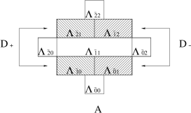
Figure 4: Illustration of the fact that whenever a fixed $\mathbb{Z}{\times}\mathbb{Z}$-grading of the spin algebra $A$ is taken, then the $\pm 1$ $\mathrm{U}(1)$ charge subspaces ${D_{+}:=\Lambda_{\bar{1}0}{\oplus}\Lambda_{\bar{2}1}}$ and ${D_{-}:=\Lambda_{\bar{0}1}{\oplus}\Lambda_{\bar{1}2}}$ can be considered as embedded Dirac bispinor spaces in $A$. Conversely: the spin algebra $A$ can be considered as a generalization of the Dirac bispinor / Clifford algebra concept.

Fourth order self-interaction potential. Relying on the symbolic Maple calculation it turns out that there are 5 linearly independent self-interaction terms, merely dependent on $\Psi$ and $\sigma_{a}^{{}_{A^{\prime}A}}$. These are all combinatorial variants of the $\mathcal{G}_{s}$-invariant form field ${\mathbf{v}(o,\sigma)\,\mathbf{L}(\cdot,\cdot)\,\mathbf{L}(\cdot,\cdot)}$. The number of 5 invariants can also be understood by taking the representation Eq.(49) of the multilinear form ${\mathbf{L}(\cdot,\cdot)\otimes\mathbf{L}(\cdot,\cdot)}$, which reads as

$$\bar{\boldsymbol{\lambda}}(\cdot,\cdot)\otimes\boldsymbol{\lambda}(\cdot,\cdot)\otimes\bar{\boldsymbol{\lambda}}(\cdot,\cdot)\otimes\boldsymbol{\lambda}(\cdot,\cdot),$$

and by subsequent enumeration of its linearly independent combinatorial contractions with ${\overline{\Psi}\otimes\overline{\Psi}\otimes\Psi\otimes\Psi}$, understood as a tensor of

$$A\otimes A\otimes A\otimes A\equiv\bar{\mathcal{A}}\otimes\mathcal{A}\otimes\bar{\mathcal{A}}\otimes\mathcal{A}\otimes\bar{\mathcal{A}}\otimes\mathcal{A}\otimes\bar{\mathcal{A}}\otimes\mathcal{A}.$$

Apart from invariance requirements, there is a clear guideline to select physically relevant combinations from the 5 invariant potential terms: the requirement of non-negativity of the potential. Two of the five invariants, based on ${\mathbf{L}\big{(}\overline{\Psi},\Psi\big{)}\,\mathbf{L}\big{(}\overline{\Psi},\Psi\big{)}}$ and on ${\mathbf{L}\big{(}\overline{\Psi},\overline{\Psi}\big{)}\,\mathbf{L}\big{(}\Psi,\Psi\big{)}}$, are easily seen to be positive semidefinite. It is not easy to judge whether the remaining three invariants can be cast to a positive semidefinite form: generally, it is known not to be a simple problem to automatically deduce if a quartic form is positive semidefinite, unless it obviously can be written as sums of squares. A possible guideline to select a preferred combination of the 5 invariant potentials could be that one requires the symmetries as all the other invariant Lagrangian terms do obey, in particular that Eq.(58) obeys. Namely, that the Lagrangian should be invariant to the shift of the top-form component according to ${\Psi\mapsto\Psi+b(\Psi)\,\mathrm{i}\,\boldsymbol{\omega}}$ with $\boldsymbol{\omega}$ being a $\mathop{\mathrm{Re}}\nolimits\big{(}M^{4}(A)\big{)}$ valued field. That requirement can be shown to uniquely select the invariant based on ${\mathbf{L}\big{(}\overline{\Psi},\Psi\big{)}\,\mathbf{L}\big{(}\overline{\Psi},\Psi\big{)}}$, namely:

$$\begin{array}[]{l}\mathrm{L}_{{}_{\mathrm{V}}}(o,\,\sigma_{a}^{{}_{A^{\prime}A}},\,\Psi,\,\nabla_{a}\Psi,\,P(\nabla)_{ab})\;:=\;\mathbf{v}(o,\sigma)\,\mathbf{L}\big{(}\overline{\Psi},\Psi\big{)}\,\mathbf{L}\big{(}\overline{\Psi},\Psi\big{)}.\cr\end{array}$$ (62)

In Section 6, we shall present a further symmetry argument, which also suggests that the above invariant Lagrangian is a preferred unique combination for a self-interaction potential term.

As mentioned before, due to the high dimensionality of the problem we were not able to formally prove that the above invariants exhaust the set of all linearly independent invariant Lagrangians, but there is strong evidence that these are all. In any case, the linear combination of the known invariants

$$\begin{array}[]{l}\mathrm{L}_{A_{\mathrm{YM}},\,A_{\mathrm{EH}},\,A_{\mathrm{D}},\,A_{\mathrm{V}}}\;:=\;A_{\mathrm{YM}}\,\mathrm{L}_{{}_{\mathrm{YM}}}\;+\;A_{\mathrm{EH}}\,\mathrm{L}_{{}_{\mathrm{EH}}}\;+\;A_{\mathrm{D}}\,\mathrm{L}_{{}_{\mathrm{D}}}\;+\;A_{\mathrm{V}}\,\mathrm{L}_{{}_{\mathrm{V}}}\cr\end{array}$$ (63)

with real coupling constants ${A_{\mathrm{YM}},A_{\mathrm{EH}},A_{\mathrm{D}},A_{\mathrm{V}}}$ provides also an invariant Lagrangian. The question naturally arises: to what degree the behavior of such a theory depends on these coupling constants? We address this question in the following.

6 The number of truly independent couplings in the toy model

In this section we show that at the classical level, 3 of the 4 independent coupling constants ${A_{\mathrm{YM}},A_{\mathrm{EH}},A_{\mathrm{D}},A_{\mathrm{V}}}$ can be eliminated by field redefinition transformations. Thus, there remains only one independent coupling constant, which can be attributed e.g. to the strength of the gravitational interaction in the model.

In order to address the question of how many of the coupling factors of the toy model are truly independent, one first needs to establish the notion of equivalence of two instances of the theory. An instance

$$\Big{(}\mathcal{M}^{\prime},\,A^{\prime}(\mathcal{M}^{\prime}),\,\mathcal{G}^{\prime}(\mathcal{M}^{\prime}),\,(A^{\prime}_{\mathrm{YM}},A^{\prime}_{\mathrm{EH}},A^{\prime}_{\mathrm{D}},A^{\prime}_{\mathrm{V}}),\,\mathrm{L}^{\prime}_{A^{\prime}_{\mathrm{YM}},\,A^{\prime}_{\mathrm{EH}},\,A^{\prime}_{\mathrm{D}},\,A^{\prime}_{\mathrm{V}}}\Big{)}$$

of the theory is defined to be equivalent to an other instance

$$\Big{(}\mathcal{M},\,A(\mathcal{M}),\,\mathcal{G}(\mathcal{M}),\,(A_{\mathrm{YM}},A_{\mathrm{EH}},A_{\mathrm{D}},A_{\mathrm{V}}),\,\mathrm{L}_{A_{\mathrm{YM}},\,A_{\mathrm{EH}},\,A_{\mathrm{D}},\,A_{\mathrm{V}}}\Big{)}$$

if and only if there exists a principal bundle isomorphism ${\mathcal{G}^{\prime}(\mathcal{M}^{\prime})\rightarrow\mathcal{G}(\mathcal{M})}$ with underlying vector bundle isomorphism ${A^{\prime}(\mathcal{M}^{\prime})\rightarrow A(\mathcal{M})}$ and underlying diffeomorphism ${\mathcal{M}^{\prime}\rightarrow\mathcal{M}}$, such that $\mathrm{L}_{A_{\mathrm{YM}},A_{\mathrm{EH}},A_{\mathrm{D}},A_{\mathrm{V}}}$ is pulled back to $\mathrm{L}^{\prime}_{A^{\prime}_{\mathrm{YM}},A^{\prime}_{\mathrm{EH}},A^{\prime}_{\mathrm{D}},A^{\prime}_{\mathrm{V}}}$, up to a nonzero real multiplier. The overall normalization can be disregarded for a classical field theory, since the Euler–Lagrange equations do not depend on the absolute normalization of the Lagrange form, and the relative hierarchy of the Noether charges is also independent of that. Assume that we have one instance of the theory with all the coupling constants ${A_{\mathrm{YM}},A_{\mathrm{EH}},A_{\mathrm{D}},A_{\mathrm{V}}}$ being nonzero. Then, by means of the above definition, all such theories are equivalent to an instance with coupling factors ${1,\frac{A_{\mathrm{EH}}}{A_{\mathrm{YM}}},\frac{A_{\mathrm{D}}}{A_{\mathrm{YM}}},\frac{A_{\mathrm{V}}}{A_{\mathrm{YM}}}}$, i.e. when the Yang–Mills coupling factor is fixed to $1$, by convention. Thus, it is enough to study theories with coupling factors ${1,A_{\mathrm{EH}},A_{\mathrm{D}},A_{\mathrm{V}}}$.

We now address the question whether some of the remaining couplings ${1,A_{\mathrm{EH}},A_{\mathrm{D}},A_{\mathrm{V}}}$ can be eliminated by field redefinition transformations. By counting the homogeneity degree of the terms of ${\mathrm{L}_{{}_{\mathrm{YM}}},\,\mathrm{L}_{{}_{\mathrm{EH}}},\,\mathrm{L}_{{}_{\mathrm{D}}},\,\mathrm{L}_{{}_{\mathrm{V}}}}$, we establish the fact that some further coupling factors can be eliminated, using a kind of “classical renormalization”, while keeping the invariant observables intact. In order to make the argument more exact, we need to formally introduce the deformation theory of Lagrangians, and thus of action functionals.

Let ${S:\mathbb{R}\times\mathcal{F}\rightarrow\mathcal{R},\,(a,f)\mapsto S(a,f)}$ be some continuously differentiable functional, with $\mathcal{F}$ being some topological affine space with a norm type topology, and $S$ taking its values in some topological vector space $\mathcal{R}$. Let us denote the underlying vector space of $\mathcal{F}$ by $\delta{\mathcal{F}}$. For instance, $S$ may be the action functional from the space of a deformation parameter ($\mathbb{R}$), and the field configuration space ($\mathcal{F}$) over some compact region of spacetime, mapping onto the real numbers (the space $\mathcal{R}$ is $\mathbb{R}$ in that case), and the underlying vector space $\delta{\mathcal{F}}$ of $\mathcal{F}$ is then the space of field variations with the uniquely and naturally defined $C^{k}$ norm topology. Over such spaces, the ordinary Fréchet differentiability, i.e. the usual notion of differentiability based on the ordo functions, is meaningful and uniquely defined. We call such a map ${(a,f)\mapsto S(a,f)}$ a deformation family of the functional ${f\mapsto S(1,f)}$.

Recall that given ${a\in\mathbb{R}}$ and ${f\in\mathcal{F}}$, the partial Fréchet derivative in the second variable ${D_{2}S(\cdot,\cdot)\big{|}_{(a,f)}}$ is a continuous linear map ${\delta{\mathcal{F}}\rightarrow\mathcal{R}}$. Given a closed subspace $\delta^{\circ}\!\mathcal{F}$ of $\delta{\mathcal{F}}$, one may consider the restriction of the above linear map to that subspace, denoted by ${D_{2}^{\delta^{\circ}\!\mathcal{F}}S(\cdot,\cdot)\big{|}_{(a,f)}}$. For instance, $\delta^{\circ}\!\mathcal{F}$ may be the subspace of field variations $\delta{\mathcal{F}}$ which vanish on the boundary of the compact region over which the action functional is considered. With that example, the equation ${D_{2}^{\delta^{\circ}\!\mathcal{F}}S(\cdot,\cdot)\big{|}_{(1,f)}=0}$ would be equivalent to the Euler–Lagrange equation of the action $S(1,\cdot)$, at a field configuration $f\in\mathcal{F}$ (variation with fixed boundary values). Let then ${F:\mathbb{R}\times\mathcal{F}\rightarrow\mathcal{F},(a,f)\mapsto F(a,f)}$ be a continuously differentiable map such that for all parameters ${a\in\mathbb{R}}$ the mapping ${f\mapsto F(a,f)}$ is one-to-one and onto, and that ${F(1,\cdot)}$ is the identity of $\mathcal{F}$. We call ${(a,f)\mapsto F(a,f)}$ a deformation family of the space $\mathcal{F}$. We then say that a deformation family ${(a,f)\mapsto S(a,f)}$ of a functional and a deformation family ${(a,f)\mapsto F(a,f)}$ of its configuration space $\mathcal{F}$ are compatible if for all parameters ${a\in\mathbb{R}}$ one has that ${S(a,F(a,\cdot))=S(1,\cdot)}$. This, for the case of an action functional, would mean that the deformation of the action is compensated by a counter-deformation of the field configuration space.

Assuming that $S$ and $F$ are compatible, one has that ${D\left(S(a,F(a,\cdot))\right)\big{|}_{f}=D_{2}\left(S(\cdot,\cdot)\right)\big{|}_{(1,f)}}$ for all ${a\in\mathbb{R}}$ and ${f\in\mathcal{F}}$. The left hand side of that equation can be reformulated via the chain rule of differentiation, thus one infers ${D_{2}(S(\cdot,\cdot))\big{|}_{(a,F(a,f))}\;D_{2}(F(\cdot,\cdot))|_{(a,f)}}={D_{2}\left(S(\cdot,\cdot)\right)\big{|}_{(1,f)}}$. We call a deformation family ${(a,f)\mapsto F(a,f)}$ of the space $\mathcal{F}$ to be regular, whenever for all parameters ${a\in\mathbb{R}}$ and configurations ${f\in\mathcal{F}}$ the ${\delta{\mathcal{F}}\rightarrow\delta{\mathcal{F}}}$ linear map ${D_{2}(F(\cdot,\cdot))\big{|}_{(a,f)}}$ is onto. Moreover, we call it regular over a closed subspace $\delta^{\circ}\!\mathcal{F}$ of $\delta{\mathcal{F}}$, whenever for all parameters ${a\in\mathbb{R}}$ and configurations ${f\in\mathcal{F}}$ the ${\delta{\mathcal{F}}\rightarrow\delta{\mathcal{F}}}$ linear map ${D_{2}(F(\cdot,\cdot))\big{|}_{(a,f)}}$ can be restricted as a ${\delta^{\circ}\!\mathcal{F}\rightarrow\delta^{\circ}\!\mathcal{F}}$ linear map which is onto. If $S$ and $F$ are compatible, and $F$ is regular over $\delta^{\circ}\!\mathcal{F}$, then from the above chain rule argument one infers that

$${D_{2}^{\delta^{\circ}\!\mathcal{F}}\!\left(S(\cdot,\cdot)\right)\big{|}_{(1,f)}=0} \;\Longrightarrow\; {D_{2}^{\delta^{\circ}\!\mathcal{F}}\!(S(\cdot,\cdot))\big{|}_{(a,F(a,f))}=0}.$$ (64)

Applying this identity to our specific case, $S$ being the action functional, this means that under such conditions, taking a field configuration ${f\in\mathcal{F}}$ which solves the Euler–Lagrange equation ${D_{2}^{\delta^{\circ}\!\mathcal{F}}(S(\cdot,\cdot))\big{|}_{(1,f)}=0}$, then for all ${a\in\mathbb{R}}$ its deformed version ${F(a,f)\in\mathcal{F}}$ is also a solution of the deformed Euler–Lagrange equation ${D_{2}^{\delta^{\circ}\!\mathcal{F}}(S(\cdot,\cdot))\big{|}_{(a,F(a,f))}=0}$. One can make a rather evident observation that whenever the deformation family of the field configurations ${a\mapsto F(a,\cdot)}$ is spacetime pointwise, then it is regular over $\delta^{\circ}\!\mathcal{F}$ (and over the entire ${\delta\mathcal{F}}$) if and only if for all ${a\in\mathbb{R}}$ the spacetime pointwise derivative of $F(a,\cdot)$ against the field configurations is onto. That is an easily testable (finite dimensional) condition, which we will use.

With the above arguments we have shown that under appropriate conditions, one can generate a flow of corresponding solutions ${a\mapsto F(a,f)}$ for a flow ${a\mapsto S(a,\cdot)}$ of theories, from a single instance of the theory ${S(1,\cdot)}$ and its solution $f$. For different parameters ${a\in\mathbb{R}}$, however, the deformed solution ${F(a,f)}$ of the deformed theory ${S(a,\cdot)}$ might eventually describe physically different configurations. For instance, from the above first principles, there is no guarantee that the physically relevant invariants, such as some relevant Noether charges of the solutions, are the same throughout the deformation family. In the following we investigate that under what additional conditions the Noether charges are constant throughout the deformation flow ${a\mapsto F(a,f)}$ of a solution.

Consider a spacetime pointwise deformation family of a Lagrangian ${a\mapsto\mathrm{L}(a,\cdot)}$ together with a spacetime pointwise regular and compatible counter-deformation ${a\mapsto F(a,\cdot)}$ of the field configuration space. We assume a Palatini-like variational principle, i.e. for a fixed ${a\in\mathbb{R}}$, the field configuration $f$ is a pair ${(v,\nabla)}$, $v$ being section of a vector bundle $V(\mathcal{M})$ (matter fields), and $\nabla$ being covariant derivative on $V(\mathcal{M})$ (combined gauge and gravitational connection). The Lagrangian is assumed to depend on three field variables, the matter fields ($v$), the matter field covariant derivatives ($\nabla_{b}v$), and the curvature ($P(\nabla)_{cd}$), and hence it is a mapping ${\big{(}a,\,(v,\,\nabla_{b}v,\,P(\nabla)_{cd})\big{)}}\mapsto{\mathrm{L}\big{(}a,\,(v,\,\nabla_{b}v,\,P(\nabla)_{cd})\big{)}}$. We shall check under what conditions the Noether current densities along the deformation family ${a\mapsto\mathrm{L}(a,\cdot)}$ are constant with respect to the deformation parameter ${a\in\mathbb{R}}$. As a shorthand notation, we will use ${\big{(}\,{}^{{}^{(a)}}\!\!v,{}^{{}^{(a)}}\!\nabla\,\big{)}}$ for the image of a field configuration ${(v,\nabla)}$ by the field deformation map ${F(a,\cdot)}$. Let $\mathsterling$ be a first order differential operator over the sections of $V(\mathcal{M})$ which generates a local vector bundle automorphism over $V(\mathcal{M})$. Let $u^{b}$ be the tangent vector field of the base manifold $\mathcal{M}$, subordinate to $\mathsterling$, describing its corresponding flow on the base manifold. Assume that for all ${a\in\mathbb{R}}$ the symmetry generator $\mathsterling$ leaves the Lagrangian ${\mathrm{L}(a,\cdot)}$ intact, i.e. that the Lagrangian ${\mathrm{L}(a,\cdot)}$ is $\mathsterling$-covariant. Assuming that ${(v,\nabla)}$ is an Euler–Lagrange solution of ${\mathrm{L}(1,\cdot)}$, then because of the above conditions, ${\big{(}\,{}^{{}^{(a)}}\!\!v,{}^{{}^{(a)}}\!\nabla\,\big{)}}$ shall also be an Euler–Lagrange solution of ${\mathrm{L}(a,\cdot)}$ for all ${a\in\mathbb{R}}$. Moreover for any fixed ${a\in\mathbb{R}}$, the volume form valued vector field

$$\begin{array}[]{l}\mathrm{J}^{b}_{\mathsterling}\left(a,\,\big{(}{}^{{}^{(a)}}\!\!v,{}^{{}^{(a)}}\!\nabla({}^{{}^{(a)}}\!\!v),P({}^{{}^{(a)}}\!\nabla)\big{)}\right):=\cr\Bigg{.}\qquad D_{2,2}^{b}\mathrm{L}\left(a,\,\big{(}{}^{{}^{(a)}}\!\!v,{}^{{}^{(a)}}\!\nabla({}^{{}^{(a)}}\!\!v),P({}^{{}^{(a)}}\!\nabla)\big{)}\right)\,\mathsterling\big{(}{}^{{}^{(a)}}\!\!v\big{)}\cr\Bigg{.}\qquad+2\,D_{2,3}^{[bc]}\mathrm{L}\left(a,\,\big{(}{}^{{}^{(a)}}\!\!v,{}^{{}^{(a)}}\!\nabla({}^{{}^{(a)}}\!\!v),P({}^{{}^{(a)}}\!\nabla)\big{)}\right)\,\left[\mathsterling,{}^{{}^{(a)}}\!\nabla_{c}\right]\cr\qquad\,-\,\mathrm{L}\left(a,\,\big{(}{}^{{}^{(a)}}\!\!v,{}^{{}^{(a)}}\!\nabla({}^{{}^{(a)}}\!\!v),P({}^{{}^{(a)}}\!\nabla)\big{)}\right)\,u^{b}\cr\end{array}$$ (65)

will be the corresponding $\mathsterling$-Noether current density, which is divergence free. (A vector density, i.e. a volume form valued vector field has a naturally defined divergence operator.) The symbols ${D_{2,1}\mathrm{L}}$, ${D_{2,2}\mathrm{L}}$, ${D_{2,3}\mathrm{L}}$ denote the spacetime pointwise partial derivative of $\mathrm{L}$ against its 2,1-th, 2,2-th and 2,3-th variable, respectively, i.e. against the matter fields, against the matter field covariant derivatives, and against the curvature. (In the above notation, the 1-st variable is reserved for the deformation parameter ${a\in\mathbb{R}}$ itself.) From the formula Eq.(65) of the Noether current density, one can directly read off a rather evident sufficient condition for ${a\mapsto\mathrm{J}^{b}_{\mathsterling}\left(a,\,\big{(}{}^{{}^{(a)}}\!\!v,{}^{{}^{(a)}}\!\nabla({}^{{}^{(a)}}\!\!v),P({}^{{}^{(a)}}\!\nabla)\big{)}\right)}$ to be constant along the deformation parameter ${a\in\mathbb{R}}$. Assume that the following conditions hold:

1. ${\big{(}a,\,(v,\,\nabla{v},\,P(\nabla))\big{)}\mapsto\mathrm{L}\big{(}a,\,(v,\,\nabla{v},\,P(\nabla))\big{)}}$ is a spacetime pointwise deformation family of the Lagrangian.

2. ${\big{(}a,\,(v,\,\nabla{v},\,P(\nabla))\big{)}\mapsto F\big{(}a,\,(v,\,\nabla{v},\,P(\nabla))\big{)}}$ is a spacetime pointwise deformation family of the field configurations which is regular.

3. the deformation family ${a\mapsto\mathrm{L}(a,\cdot)}$ and ${a\mapsto F(a,\cdot)}$ are compatible, i.e. for any field configuration ${(v,\nabla)}$ one has ${\mathrm{L}\left(a,\,\big{(}{}^{{}^{(a)}}\!\!v,{}^{{}^{(a)}}\!\nabla({}^{{}^{(a)}}\!\!v),P({}^{{}^{(a)}}\!\nabla)\big{)}\right)=\text{\emph{const}}}$ along ${a\in\mathbb{R}}$.

4. for all deformation parameters $a\in\mathbb{R}$ the symmetry generator $\mathsterling$ leaves the Lagrangian ${\mathrm{L}(a,\cdot)}$ invariant, i.e. the Lagrangian ${\mathrm{L}(a,\cdot)}$ is $\mathsterling$-covariant.

5. for all deformation parameters ${a\in\mathbb{R}}$ the symmetry generator $\mathsterling$ leaves the deformation mapping ${F(a,\cdot)}$ invariant, i.e. ${F(a,\cdot)}$ is $\mathsterling$-covariant.

6. one has the compatibility condition that for any field configurations ${(v,\nabla)}$ and ${(v^{\prime},\nabla^{\prime})}$

   $$\begin{array}[]{rl}D_{2,2}^{b}\mathrm{L}\left(a,\,\big{(}{}^{{}^{(a)}}\!\!v,{}^{{}^{(a)}}\!\nabla({}^{{}^{(a)}}\!\!v),P({}^{{}^{(a)}}\!\nabla)\big{)}\right)\,\big{(}{}^{{}^{(a)}}\!\!v^{\prime}{-}{}^{{}^{(a)}}\!\!v\big{)}&\cr+\,\Big{.}2\,D_{2,3}^{[bc]}\mathrm{L}\left(a,\,\big{(}{}^{{}^{(a)}}\!\!v,{}^{{}^{(a)}}\!\nabla({}^{{}^{(a)}}\!\!v),P({}^{{}^{(a)}}\!\nabla)\big{)}\right)\,\big{(}{}^{{}^{(a)}}\!\nabla^{\prime}_{c}{-}\!{}^{{}^{(a)}}\!\nabla_{c}\big{)}&\;=\;\text{\emph{const}}\cr\end{array}$$

   holds along ${a\in\mathbb{R}}$.

Then, for all the Euler–Lagrange solutions ${(v,\nabla)}$ of ${\mathrm{L}(1,\cdot)}$ the corresponding deformed field configuration ${\big{(}\,{}^{{}^{(a)}}\!\!v,{}^{{}^{(a)}}\!\nabla\,\big{)}}$ is an Euler–Lagrange solution of the deformed Lagrangian ${\mathrm{L}(a,\cdot)}$ for any ${a\in\mathbb{R}}$, moreover the Noether current density ${\mathrm{J}^{b}_{\mathsterling}\left(a,\,\big{(}{}^{{}^{(a)}}\!\!v,{}^{{}^{(a)}}\!\nabla({}^{{}^{(a)}}\!\!v),P({}^{{}^{(a)}}\!\nabla)\big{)}\right)}$ is constant along the deformation parameter ${a\in\mathbb{R}}$.

Using the above formalism for the deformation of a theory, one can generalize the notion of equivalence of instances of a theory with different coupling factors. We define instances of a theory within a deformation family to be equivalent in the generalized sense, if there exists a regular compatible counter-deformation map of the field configurations, for which also the $\mathsterling$-Noether current density is constant along the deformation family, for all the vector bundle automorphism generators $\mathsterling$, respecting the structure group. The rationale behind this notion of equivalence is that one can generate the corresponding solutions of the deformed instances of the theory from each-other, moreover these corresponding solutions will have the same Noether charges for all the fundamental symmetry generators. Therefore, it seems to be rational to regard such a deformation family as describing the same physics throughout the flow of the deformation parameter. The sufficient conditions (i)–(vi) outlined above, are useful tools for recognizing such generalized equivalence of theory instances, and will be applied in the following to our toy model in order to eliminate some of the coupling factors.

Using the above notions, one can see that an instance of our toy model with nonvanishing coupling coefficients ${1,\,A_{\mathrm{EH}},\,A_{\mathrm{D}},\,A_{\mathrm{V}}}$ is equivalent in the generalized sense to an instance with couplings ${1,\,A_{\mathrm{EH}}/a^{2},\,A_{\mathrm{D}}/a^{3},\,A_{\mathrm{V}}/a^{4}}$. That is simply seen by observing the homogeneity degree of the invariant Lagrangians in the soldering form $\sigma_{b}^{{}_{B^{\prime}B}}$, from which one infers that a deformation ${a\mapsto\mathrm{L}_{A_{\mathrm{YM}},\,A_{\mathrm{EH}}/a^{2},\,A_{\mathrm{D}}/a^{3},\,A_{\mathrm{V}}/a^{4}}}$ of the Lagrangian may be compensated by a compatible counter-deformation ${(\sigma_{b}^{{}_{B^{\prime}B}},\,\Psi,\,\nabla_{c})\mapsto(a\,\sigma_{b}^{{}_{B^{\prime}B}},\,\Psi,\,\nabla_{c})}$, which satisfies (i)–(vi) for all ${a\neq 0}$. Choosing specifically ${a=A_{\mathrm{D}}^{{}_{1/3}}}$, we arrive at the conclusion that such an instance of the theory is equivalent to the instance ${1,\,A_{\mathrm{EH}}/A_{\mathrm{D}}^{{}_{2/3}},\,1,\,A_{\mathrm{V}}/A_{\mathrm{D}}^{{}_{4/3}}}$. It is thus enough to study instances of the theory with couplings $1,\,A_{\mathrm{EH}},\,1,\,A_{\mathrm{V}}$.

Further applying the above deformation theory, one can eliminate another independent coupling constant from the set ${1,\,A_{\mathrm{EH}},\,1,\,A_{\mathrm{V}}}$. For that, one needs to use the fact that both the Yang–Mills-like term, the Dirac-like term and the Einstein–Hilbert-like term is invariant to an affine shift transformation ${\Psi\mapsto\Psi+b(\Psi)\,\mathrm{i}\,\boldsymbol{\omega}}$ with $\boldsymbol{\omega}$ being a ${\mathop{\mathrm{Re}}\nolimits\big{(}M^{4}(A)\big{)}}$ valued field. In the previous section we suggested this symmetry requirement to be imposed also on the self-interaction term $\mathrm{L}_{{}_{\mathrm{V}}}$, in which case the only surviving potential term can be Eq.(62). We now suggest a further symmetry argument to support that requirement. One may observe that the field deformation family

$$\begin{array}[]{l}\Big{(}\sigma_{b}^{{}_{B^{\prime}B}},\,\Psi,\,\nabla_{c}\Big{)}\;\longmapsto\;\Big{(}{}^{{}^{(a)}}\!\sigma_{b}^{{}_{B^{\prime}B}},\,{}^{{}^{(a)}}\!\!\Psi,\,{}^{{}^{(a)}}\!\nabla_{c}\Big{)}:=\Big{(}\sigma_{b}^{{}_{B^{\prime}B}},\,\big{(}\Psi+(a{-}1)\tfrac{1}{2\,b(\overline{\Psi})}\mathbf{L}(\overline{\Psi},\Psi)\big{)},\,\nabla_{c}\Big{)}\end{array}$$ (66)

satisfies (i)–(vi) for all ${a\neq 0}$, moreover it leaves the Yang–Mills-like term as well as the Dirac-like term invariant, whereas it acts as a scaling on the quadratic expression ${\Psi\mapsto\mathbf{L}\big{(}\overline{\Psi},\Psi\big{)}}$: one has the identity ${\mathbf{L}\big{(}\overline{{}^{{}^{(a)}}\!\!\Psi},{}^{{}^{(a)}}\!\!\Psi\big{)}=a\,\mathbf{L}(\overline{\Psi},\Psi)}$. Therefore, it acts on the Einstein–Hilbert-like term as a scaling transformation by $a$. On the potential term Eq.(62), which is proportional to $\mathbf{L}(\overline{\Psi},\Psi)^{2}$, the pertinent field deformation acts as a scaling by $a^{2}$. With these conditions, the instance of the theory with couplings ${1,\,A_{\mathrm{EH}},\,1,\,A_{\mathrm{V}}}$ is equivalent in the generalized sense to an instance ${1,\,A_{\mathrm{EH}}/a,\,1,\,A_{\mathrm{V}}/a^{2}}$, specifically to ${1,\,1,\,1,\,A_{\mathrm{V}}/A_{\mathrm{EH}}^{2}}$. Thus, it is enough to study the theory with couplings ${1,\,1,\,1,\,A_{\mathrm{V}}}$, i.e. with a single free coupling factor $A_{\mathrm{V}}$, describing the intensity of the self-interaction. Alternatively, one may transform this one free parameter to the pre-factor of the Einstein–Hilbert-like action, in which case it is enough to consider couplings ${1,\,A_{\mathrm{EH}},\,1,\,\pm 1}$. Since only a single coupling is left as a free parameter, such a toy model can be considered as unified.

The flat spacetime limit of the toy model can be deduced from the Lagrangian, when the instance of the theory with couplings ${1,\,A_{\mathrm{EH}},\,1,\,\pm 1}$ is considered at the limit ${A_{\mathrm{EH}}\rightarrow\infty}$. (Here, the coupling $A_{\mathrm{EH}}$ plays the role of scaling ${(\text{Planck length})^{-2}}$, so in order to switch off the gravity, that has to go to infinity.) It is seen, that in the flat spacetime limit, the theory is left with no freely adjustable coupling constants.

Remark 6.1.

Since the model turns out to have a single independent coupling, it is quite natural to ask the question about the remaining degrees of freedom of the matter field sector after a gauge fixing. Initially, a section $\Psi$ of the spin algebra bundle $A(\mathcal{M})\equiv{\Lambda\big{(}\bar{S}^{*}(\mathcal{M})\big{)}\otimes\Lambda\big{(}S^{*}(\mathcal{M})\big{)}}$ can be represented by a tuple of spinor-tensor fields

$$\begin{array}[]{l}\Psi\equiv\Big{(}\phi,\,\bar{\xi}_{{}_{(+)A^{\prime}}},\,\xi_{{}_{(-)A}},\,\bar{\varepsilon}_{{}_{(+)A^{\prime}B^{\prime}}},\,v{}_{{}_{A^{\prime}B}},\,\varepsilon_{{}_{(-)AB}},\,\bar{\chi}_{{}_{(+)A^{\prime}B^{\prime}C}},\,\chi_{{}_{(-)C^{\prime}AB}},\,\omega_{{}_{A^{\prime}B^{\prime}AB}}\Big{)}.\cr\end{array}$$

By a gauge transformation with the component $\mathbb{C}^{{}^{\times}}$ of $\mathcal{G}$, one can fix a gauge such that $b(\Psi)=1$, i.e. ${\phi=1}$ in the above representation. Then, by the $\mathrm{H}_{3}(\mathbb{C})$ part of $\mathcal{G}$, one can choose a gauge that for instance ${\xi_{{}_{(-)A}}=0}$ and ${\varepsilon_{{}_{(-)AB}}=0}$ holds (“Dirac sea gauge”, i.e. only the net fermion content is present in the description). One can then use the affine symmetry ${\Psi\mapsto\Psi+b(\Psi)\,\mathrm{i}\,\boldsymbol{\omega}}$ with $\boldsymbol{\omega}$ being a ${\mathop{\mathrm{Re}}\nolimits\big{(}M^{4}(A)\big{)}}$ valued field. That can make sure that in the above gauge, the top form $\omega_{{}_{A^{\prime}B^{\prime}AB}}$ is hermitian. Finally, the $\mathrm{D}(1)$ component of $\mathcal{G}$ can be used to fix the scale of the top form, so that ${\omega_{{}_{A^{\prime}B^{\prime}AB}}=\boldsymbol{\omega}_{{}_{A^{\prime}B^{\prime}AB}}}$, where $\boldsymbol{\omega}_{{}_{A^{\prime}B^{\prime}AB}}$ is a fixed prescribed (non-dynamical) hermitian top form. (In a GR-like formalism, on would write ${\boldsymbol{\omega}_{{}_{A^{\prime}B^{\prime}AB}}=\pm\,\bar{\boldsymbol{\epsilon}}_{{}_{A^{\prime}B^{\prime}}}{\otimes}\,\boldsymbol{\epsilon}_{{}_{AB}}}$ with $\boldsymbol{\epsilon}_{{}_{AB}}$ fixed.) In the gauge field sector, due to the affine shift symmetry ${\nabla_{b}\mapsto\nabla_{b}+C_{b}}$, with $C_{b}$ being a ${\mathbb{C}^{{}^{\times}}\times\big{(}\mathrm{H}_{3}(\mathbb{C})\rtimes\mathrm{D}(1)\big{)}}$ charged gauge potential, only the $\mathrm{U}(1)$ and $\mathrm{SL}(2,\mathbb{C})$ sector of the connection gives contribution.

Remark 6.2.

The fact that the Lagrangian admits an internal symmetry implies the existence of a corresponding Noether current, which is conserved on-shell, i.e. for fields satisfying the Euler–Lagrange equations. If in addition to the internal symmetry, the Lagrangian is invariant to shifts of the connection $\nabla_{d}\mapsto\nabla_{d}+C_{d}$ with $C_{d}$ valued in an ideal $\mathfrak{i}$ of the internal symmetry Lie algebra, then one can show that Noether currents corresponding to symmetries $\mathfrak{i}$ vanish on-shell. In our model, this implies the (on-shell) vanishing of the ${\mathbb{C}^{{}^{\times}}\times\big{(}\mathrm{H}_{3}(\mathbb{C})\rtimes\mathrm{D}(1)\big{)}}$ Noether current. For the case of the ordinary Dirac Lagrangian, discussed in Section 3, this implies the (on-shell) vanishing of the Noether current associated to the dilatation charges. Despite the fact that nilpotent symmetries do not provide additional nonzero conserved charges, they do constrain the matter content and the set of allowed coupling constants.

7 Concluding remarks

In this paper a toy model of a unified general relativistic gauge theory is constructed which exhibits a curious behavior: not all its local internal symmetry generators, which act locally and faithfully on the matter fields, are accompanied by corresponding gauge boson fields. As an introductory example it was shown that already the ordinary Dirac kinetic Lagrangian exhibits an extremely simplified version for such behavior: the gauge boson field corresponding to an internal dilatation symmetry does not give rise to any physically observable fields. In other words: the Lagrangian has a hidden affine symmetry, namely it is invariant with respect to an affine shift of the dilatation gauge connection. We showed that such behavior can also be exhibited by more complicated internal symmetry groups, and even by indecomposable (unified) ones. The necessary condition, however, is that these “exotic” symmetry generators, whose gauge boson fields can be transformed out, span an $\mathop{\mathrm{ad}}\nolimits$-invariant sub-Lie algebra of the internal symmetries. Due to a general structural theorem of Lie algebras (Levi–Mal’cev decomposition), this implies that only theories having some nilpotent internal symmetry generators besides the usual compact ones can show such behavior. We have constructed a Lagrangian that exhibits these properties. The symmetries of the constructed theory, to linearized order, has the structure of a unified group, with compact, Poincaré and nilpotent components, the latter part acting as a “glue” in the unification.

Heuristically speaking, the constructed model describes the field equations of a classical field, which spacetime pointwise has degrees of freedom similar to a second quantized fermionic theory, i.e. with pointwise degrees of freedom obeying Pauli principle. As such, it may be a kind of semiclassical limit of a QFT-like model. In this QFT heuristic picture, besides the usual compact gauge, Lorentz and dilatation symmetries, the theory is symmetric to the transformation when equal amount of fermions and charge conjugate fermions are injected into a configuration spacetime pointwise, and this happens to be isomorphic to a pointwise $\mathrm{H}_{3}(\mathbb{C})$ Heisenberg internal group action. It also turns out that the “exotic”, $\mathrm{H}_{3}(\mathbb{C})$ gauge fields can be completely transformed out from the theory due to the extra affine shift symmetry on the connection, which is a symmetry similar to what ordinary Dirac equation exhibits against the dilatation gauge fields. Thus, the nilpotent symmetries $\mathrm{H}_{3}(\mathbb{C})$, necessary for the unification, do act locally and faithfully on the matter fields, without being accompanied by physical gauge boson fields.

Appendix

Appendix A On the structure of generic Lie groups and Lie algebras

As it is well known, the universal covering group of a connected Lie group is uniquely characterized by its Lie algebra, which can be studied by purely algebraic methods. Thus, for studying Lie groups it is important to first understand the structure of Lie algebras. In the following we shall recall some general known facts concerning the structure of finite dimensional real Lie algebras. Not all of these are well known in the folklore of gauge theory literature for model building, since in the traditional model building, only semisimple or reductive Lie algebras are considered.

A.1 Ideal, semi-direct sum, direct sum

A subspace $\mathfrak{i}$ of a Lie algebra $\mathfrak{e}$ is said to be an ideal if $[x,y]$ belongs to $\mathfrak{i}$ for all $x\in\mathfrak{e}$ and $y\in\mathfrak{i}$. Notice that this condition is strictly more restrictive than the requirement of $\mathfrak{i}$ being a sub-Lie algebra of $\mathfrak{e}$. An example for an ideal is the translation generator sub-Lie algebra inside the Lie algebra of the Poincaré group, while the Lorentz generator sub-Lie algebra is not an ideal within, merely a sub-Lie algebra. The notion of ideal is arguably the most important concept in the theory of Lie algebras. The usual notation $\mathop{\mathrm{ad}}\nolimits_{x}y:=[x,y]$ shall occasionally be applied ($x,y\in\mathfrak{e}$) in the following.

For every ideal $\mathfrak{i}\subset\mathfrak{e}$ one can always find a (non-unique) complementary linear subspace, i.e. a linear subspace $C\subset\mathfrak{e}$ such that $\mathfrak{i}\cap C=\{0\}$ and $\mathfrak{i}+C=\mathfrak{e}$. In the Lie algebra theory literature, such disjoint linear sum, being simply the vector space sense direct sum, is often denoted as $\mathfrak{e}=\mathfrak{i}\dotplus C$. Given an ideal $\mathfrak{i}$, in general there need not exist a complementary subspace which is also a sub-Lie algebra of $\mathfrak{e}$. Whenever such a complementary sub-Lie algebra $\mathfrak{c}$ does exist, we say that $\mathfrak{e}$ is a semi-direct sum of $\mathfrak{i}$ with $\mathfrak{c}$, and denote it by $\mathfrak{e}=\mathfrak{i}\mathbin{\hbox to0.0pt{$\Leftcircle$\hss}{+}}\mathfrak{c}$. For instance, the Poincaré Lie algebra is a semi-direct sum of the translation and of the Lorentz Lie algebra. If the complementing sub-Lie algebra $\mathfrak{c}$ is also an ideal, then elements of $\mathfrak{i}$ commute with elements of $\mathfrak{c}$, and $\mathfrak{e}$ is said to be a direct sum of $\mathfrak{i}$ and $\mathfrak{c}$, denoted by $\mathfrak{e}=\mathfrak{i}\oplus\mathfrak{c}$. For instance, the Standard Model (SM) internal Lie algebra is a direct sum $\mathfrak{u}(1)\oplus\mathfrak{su}(2)\oplus\mathfrak{su}(3)$. On the other hand, for instance the Poincaré Lie algebra is a semi-direct sum, but not a direct sum of the translation and of the Lorentz Lie algebra. When a Lie algebra is not a direct sum of other smaller Lie algebras, it is called direct-indecomposable, or simply indecomposable, or in physics it is called unified. The GUT strategy aims at finding a field theoretical description of particle physics with a unified internal symmetry group.

A.2 A measure of non-commutativity: abelian, nilpotent, solvable, and semisimple Lie algebras

It is natural to cathegorize Lie algebras according to the degree of their non-commutativity. Quite naturally, the least non-commutative Lie algebras $\mathfrak{e}$ are the abelian ones, i.e. the ones satisfying $[\mathfrak{e},\mathfrak{e}]=\{0\}$, or equivalently, which satisfy $\mathop{\mathrm{ad}}\nolimits_{x}=0$ for all $x\in\mathfrak{e}$. A next, slightly less commutative class of Lie algebras is the class of nilpotent Lie algebras. Their defining property is that the so-called lower central series terminates in a finite number of steps: with the definition $\mathfrak{e}^{1}:=\mathfrak{e}$, $\;\mathfrak{e}^{k+1}:=[\mathfrak{e},\mathfrak{e}^{k}]$, one has that $\mathfrak{e}^{k}=\{0\}$ for some finite non-negative integer $k$. It is known (Engel’s theorem) Snobl2014 ; Onishchik1990 ; IseTakeuchi1991 ; Jacobson1962 that this condition is equivalent to the property that operator $\mathop{\mathrm{ad}}\nolimits_{x}$ is nilpotent for every $x\in\mathfrak{e}$, hence the name. Such Lie algebras play a role in physics, for instance in SUSY. An even less commutative class of Lie algebras is the class of solvable Lie algebras, which satisfy the property that their so-called derived series vanish in finite steps: with the definition $\mathfrak{e}^{(0)}:=\mathfrak{e}$, $\;\mathfrak{e}^{(k+1)}:=[\mathfrak{e}^{(k)},\mathfrak{e}^{(k)}]$ one has that $\mathfrak{e}^{(k)}=\{0\}$ for some finite non-negative integer $k$. The structure of solvable Lie algebras is slightly more complex than that of nilpotent ones. One could say, that the least commutative Lie algebras are the semisimple ones, which are defined by the property that they do not contain solvable ideals other than the trivial $\{0\}$. Usually in gauge theory only semisimple Lie algebras, e.g. direct sums of $\mathfrak{su}(N)$, are considered, along with abelian ones, which are always direct sums of some copies of the $\mathfrak{u}(1)$. Typically, general Lie algebras, possibly containing nilpotent or solvable component, are not used for field theory model building. In the present paper we address this more general possibility, and also discuss the rationale behind the traditional approach in gauge theory, while pointing out possible loopholes within.

A.3 Structure of general Lie algebras: the Levi–Mal’cev decomposition theorem

In every Lie algebra $\mathfrak{e}$ there exists a very distinguished ideal: the solvable ideal of the largest possible dimension, which is called the radical of $\mathfrak{e}$ and is denoted by $\mathop{\mathrm{rad}}\nolimits(\mathfrak{e})$. A further distinguished ideal is the largest dimensional nilpotent ideal, called the nilradical of $\mathfrak{e}$ and is denoted by $\mathop{\mathrm{nil}}\nolimits(\mathfrak{e})$. By construction, the radical and nilradical are unique, and one always has $\mathop{\mathrm{nil}}\nolimits(\mathfrak{e})\subset\mathop{\mathrm{rad}}\nolimits(\mathfrak{e})$. One of the foundational results about Lie algebras is the Levi–Mal’cev decomposition theorem Snobl2014 ; Onishchik1990 ; IseTakeuchi1991 ; Jacobson1962 , which states that the radical does admit a complementary sub-Lie algebra $\mathfrak{l}$, called Levi factor. That is, one has the semi-direct sum splitting Eq.(1), where the Levi factor $\mathfrak{l}$ is semisimple and isomorphic to the quotient Lie algebra $\frac{\mathfrak{e}}{\mathop{\mathrm{rad}}\nolimits(\mathfrak{e})}$. As such, the Levi factors are isomorphic to each other, but they are not a uniquely determined embedded sub-Lie algebra in $\mathfrak{e}$. However, the choice of a Levi factor is unique up to an inner automorphism, defined by the conjugation by the exponential of $\mathop{\mathrm{ad}}\nolimits_{z}$ for some element $z\in\mathop{\mathrm{nil}}\nolimits(\mathfrak{e})$. In this sense Levi factors are essentially unique. Also, a side result of the Levi–Mal’cev theorem is that any semisimple sub-Lie algebra of $\mathfrak{e}$ must be contained within a Levi factor, i.e. a Levi factor is the maximal semisimple sub-Lie algebra with respect to the inclusion relation. An enlightening example of Levi–Mal’cev decomposition is provided by the Lie algebra of the Poincaré group Eq.(2), in which case, the radical coincides with the nilradical, and it is abelian. As outlined in Laszlo2017 , the Lie algebra of the super-Poincaré group can also be considered as an example to the Levi–Mal’cev decomposition, with a non-abelian, but two-step nilpotent radical.

Results above indicate that constructive characterization of the radical, nilradical and Levi factor is quite important. That can be done via Cartan’s criterion Snobl2014 ; Onishchik1990 ; IseTakeuchi1991 ; Jacobson1962 , which employs the well known notion of Killing form. The Killing form $K(x,y):=\mathop{\mathrm{Tr}}\nolimits\left(\mathop{\mathrm{ad}}\nolimits_{x}\mathop{\mathrm{ad}}\nolimits_{y}\right)$ for $x,y\in\mathfrak{e}$ is an invariant symmetric bilinear form, i.e. is a naturally given scalar product on $\mathfrak{e}$ (possibly of indefinite signature and possibly degenerate). The statement of Cartan’s criterion can be formulated as: (i) the radical $\mathop{\mathrm{rad}}\nolimits(\mathfrak{e})$ is the subspace within $\mathfrak{e}$ which is orthogonal to $[\mathfrak{e},\mathfrak{e}]$ with respect to the Killing form, moreover (ii) Levi factor $\mathfrak{l}$ of $\mathfrak{e}$ is a maximal dimensional sub-Lie algebra on which the Killing form is nondegenerate.

Another important property of semisimple Lie algebras, and hence of the Levi factor of every Lie algebra, is the Weyl’s theorem on complete reducibility Snobl2014 ; Onishchik1990 ; IseTakeuchi1991 ; Jacobson1962 . Its consequence is that every ideal of a semisimple Lie algebra has a complementing ideal, and therefore any semisimple Lie algebra is a direct sum of simple Lie algebras: these are Lie algebras which do not have any ideals apart from the trivial ones, i.e. apart from the zero and the entire Lie algebra. Knowing the above properties, one can draw the following “big picture” of the structure of general Lie algebras:

$$\underbrace{\mathfrak{e}}_{\begin{subarray}{c}\text{arbitrary}\\ \text{Lie algebra}\end{subarray}} \;=\; \underbrace{\mathop{\mathrm{rad}}\nolimits(\mathfrak{e})}_{\begin{subarray}{c}\text{maximal}\\ \text{solvable ideal,}\\ \text{Killing form}\\ \text{is degenerate}\\ \text{(\emph{radical})}\end{subarray}}\mathbin{\hbox to0.0pt{$\Leftcircle$\hss}{+}}\;\underbrace{\overbrace{\mathfrak{l}_{1}}^{\begin{subarray}{c}\text{no ideals}\\ \text{inside}\\ \text{(\emph{simple})}\end{subarray}}\!\!{\oplus}{\dots}{\oplus}\!\!\overbrace{\mathfrak{l}_{n}}^{\begin{subarray}{c}\text{no ideals}\\ \text{inside}\\ \text{(\emph{simple})}\end{subarray}}}_{\begin{subarray}{c}\text{maximal}\\ \text{semisimple sub-Lie algebra,}\\ \text{Killing form}\\ \text{is nondegenerate}\\ \text{(\emph{Levi factor}})\end{subarray}}.$$ (67)

The structure of simple Lie algebras is rather thoroughly explored: they are classified by the Dynkin diagrams. In physics literature by the standard theory of Lie algebras, mostly the theory of simple Lie algebras is meant. If nontrivial radicals are also allowed, the classification theory of simple Lie algebras is not enough, and one needs to look at the possible structure of solvable Lie algebras as well.

A.4 Structure of radicals of Lie algebras

The classification of all finite dimensional real or complex Lie algebras with nonvanishing radical is unresolved, moreover is known to be a “wild problem” in mathematics. Complete classification exists only for low dimensional Lie algebras. There are however, some results on the generalities of the possible structure of such Lie algebras. For completeness, we recall some of these results, mostly from Snobl2010 ; Snobl2014 .

Let us consider a finite dimensional real Lie algebra with Levi–Mal’cev decomposition Eq.(1). The identities $\mathop{\mathrm{nil}}\nolimits(\mathfrak{e})\subset\mathop{\mathrm{rad}}\nolimits(\mathfrak{e})$, $[\mathfrak{e},\mathop{\mathrm{rad}}\nolimits(\mathfrak{e})]\subset\mathop{\mathrm{nil}}\nolimits(\mathfrak{e})$, $[\mathfrak{l},\mathfrak{l}]=\mathfrak{l}$ are well known. If $\mathfrak{e}$ is indecomposable, i.e. not a direct sum of smaller Lie algebras, then the representation of $\mathfrak{l}$ by $\mathop{\mathrm{ad}}\nolimits$ on $\mathop{\mathrm{rad}}\nolimits(\mathfrak{e})$ is known to be faithful Snobl2014 . From now on, assume that $\mathfrak{e}$ is indecomposable. Then, one has the result by Turkowski, recalled in Snobl2010 ; Snobl2014 , that there exists a (non unique) subspace $q$ within $\mathop{\mathrm{rad}}\nolimits(\mathfrak{e})$ complementing the ideal $\mathop{\mathrm{nil}}\nolimits(\mathfrak{e})$, i.e. $\mathop{\mathrm{rad}}\nolimits(\mathfrak{e})=\mathop{\mathrm{nil}}\nolimits(\mathfrak{e})\dotplus q$, such that the action of $\mathfrak{l}$ by the $\mathop{\mathrm{ad}}\nolimits$ on $q$ vanishes. The subspace $q$, however, may not always be a sub-Lie algebra, i.e. the preceding $\dotplus$ may not be a semi-direct sum $\mathbin{\hbox to0.0pt{$\Leftcircle$\hss}{+}}$. Whenever the subspace $q$ is sub-Lie algebra, then it is necessarily abelian: $[q,q]=\{0\}$. The structure of the nilradical can be characterized by results of Šnobl Snobl2010 ; Snobl2014 : there exists a (non unique) tuple of complementing subspaces $m_{1},\dots,m_{k}$ within $\mathop{\mathrm{nil}}\nolimits(\mathfrak{e})$, such that $\mathop{\mathrm{nil}}\nolimits(\mathfrak{e})=m_{k}\dotplus\dots\dotplus m_{1}$, with $\mathop{\mathrm{nil}}\nolimits(\mathfrak{e})^{j}=m_{j}\dotplus\mathop{\mathrm{nil}}\nolimits(\mathfrak{e})^{j+1}$, and $m_{j+1}\subset[m_{1},m_{j}]$, and $\mathop{\mathrm{ad}}\nolimits_{\mathfrak{l}}m_{j}\subset m_{j}$ ($j=1,{\dots},k$), moreover $\mathfrak{l}$ acts by $\mathop{\mathrm{ad}}\nolimits$ on $m_{1}$ faithfully. All this can be summarized in a “big picture” of the structure of indecomposable Lie algebras:

$$\begin{array}[]{c}\qquad\qquad\text{\tiny(arrows: nonvanishing, faithful, adjoint action)}\cr\cr\underbrace{\mathfrak{e}}_{\begin{subarray}{c}\text{arbitrary}\\ \text{indecomp.}\\ \text{Lie algebra}\end{subarray}}=\;\underbrace{\!\!\underbrace{\overset{{}^{\leavevmode\hbox to4.67pt{\vbox to4.67pt{\text{[drawing]}}}}}{m_{k}}{\dotplus}{\dots}{\dotplus}\overset{{}^{\leavevmode\hbox to4.67pt{\vbox to4.67pt{\text{[drawing]}}}}}{m_{1}}}_{\begin{subarray}{c}\mathop{\mathrm{nil}}\nolimits(\mathfrak{e})\text{, the maximal}\\ \text{nilpotent ideal,}\\ \text{Killing form is zero}\\ \text{(\emph{nilradical})}\end{subarray}}\!\!\!\!\dotplus\,\overset{{}^{\leavevmode\hbox to4.67pt{\vbox to4.67pt{\text{[drawing]}}}}}{q}}_{\begin{subarray}{c}\mathop{\mathrm{rad}}\nolimits(\mathfrak{e})\text{, the maximal}\\ \text{solvable ideal,}\\ \text{Killing form}\\ \text{is degenerate}\\ \text{(\emph{radical})}\end{subarray}}\;\;\mathbin{\hbox to0.0pt{$\Leftcircle$\hss}{+}}\!\!\underbrace{\underbrace{\overset{\leavevmode\hbox to6.67pt{\vbox to6.67pt{\text{[drawing]}}}}{\mathfrak{l}_{1}}}_{\begin{subarray}{c}\text{no ideals}\\ \text{inside}\\ \text{(\emph{simple})}\end{subarray}}\!\!\!\!{\oplus}{\dots}{\oplus}\!\!\!\!\underbrace{\overset{\leavevmode\hbox to6.67pt{\vbox to6.67pt{\text{[drawing]}}}}{\mathfrak{l}_{n}}}_{\begin{subarray}{c}\text{no ideals}\\ \text{inside}\\ \text{(\emph{simple})}\end{subarray}}}_{\begin{subarray}{c}\mathfrak{l}\text{, a maximal}\\ \text{semisimple sub-Lie algebra,}\\ \text{Killing form}\\ \text{is nondegenerate}\\ \text{(\emph{Levi factor}})\end{subarray}}.\cr\end{array}\leavevmode\hbox to1.5pt{\vbox to15.1pt{\text{[drawing]}}}\leavevmode\hbox to0.4pt{\vbox to11.16pt{\text{[drawing]}}}\leavevmode\hbox to0.4pt{\vbox to11.16pt{\text{[drawing]}}}\leavevmode\hbox to0.4pt{\vbox to11.16pt{\text{[drawing]}}}\leavevmode\hbox to0.4pt{\vbox to11.16pt{\text{[drawing]}}}\leavevmode\hbox to0.4pt{\vbox to11.16pt{\text{[drawing]}}}$$ (68)

Remark A.1.

A further constraint on the structure of radical is a theorem of Šnobl (2010) Snobl2010 : if $\mathfrak{e}$ is an indecomposable Lie algebra over $\mathbb{C}$, and its Levi factor $\mathfrak{l}$ acts irreducibly by $\mathop{\mathrm{ad}}\nolimits$ on the top subspace $m_{1}$ of $\mathop{\mathrm{nil}}\nolimits(\mathfrak{e})$, then the complementing subspace $q$ to the nilradical $\mathop{\mathrm{nil}}\nolimits(\mathfrak{e})$ within the radical $\mathop{\mathrm{rad}}\nolimits(\mathfrak{e})$ is $0$ or $1$ complex dimensional. In the latter case, one has that $q\cong\boldsymbol{\mathtt{d}}(1){\oplus}\,\mathfrak{u}(1)$, i.e. $q$ closes as an (abelian) sub-Lie algebra. Also, it is seen that under such conditions, there can be maximum one copy of the $\mathfrak{u}(1)$ component within. (This might remind us about the structure of the Standard Model Lie algebra, which also has merely one copy of $\mathfrak{u}(1)$, and thus well may be the factor $\frac{\mathfrak{e}}{\mathop{\mathrm{nil}}\nolimits(\mathfrak{e})}$ of some larger indecomposable Lie algebra $\mathfrak{e}$.)

Remark A.2.

In the case when $\mathfrak{e}$ is the Lie algebra of a real linear algebraic group, there are some further constraints on the structure of $\mathop{\mathrm{rad}}\nolimits(\mathfrak{e})$. Such constraints are implied by Mostow’s decomposition theorem of linear algebraic groups borel1991 : a connected real linear algebraic group can be decomposed as a semi-direct product of an idempotent normal subgroup and of a so-called reductive subgroup.

A.5 Lie algebras in traditional model building: quadratic, reductive and compact Lie algebras

As outlined, every Lie algebra has an $\mathop{\mathrm{ad}}\nolimits$-invariant, but possibly indefinite and possibly degenerate scalar product: the Killing form. It is often of interest to consider Lie algebras with a nondegenerate (possibly indefinite) invariant scalar product. Such Lie algebras are called quadratic. Quadratic Lie algebras play a natural role as internal Lie algebras in gauge theory, since the nondegeneracy of the invariant scalar product would ensure that all gauge fields would propagate. Not all possible quadratic Lie algebras are fully classified as of now.

An important class of quadratic Lie algebras are called reductive. These can be defined by the following equivalent properties: (i) its adjoint representation is completely reducible (direct sum of irreducible ones), (ii) it admits a faithful finite dimensional completely reducible representation, (iii) its radical coincides with its center, (iv) it is a direct sum of an abelian ideal and of a semisimple Lie algebra. As such, a reductive Lie algebra $\mathfrak{e}$ has the structure: $\mathfrak{e}=\mathfrak{u}(1){\oplus}{\dots}{\oplus}\,\mathfrak{u}(1){\oplus}\,\mathfrak{l}_{1}{\oplus}{\dots}{\oplus}\,\mathfrak{l}_{n}$, where the components $\mathfrak{l}_{1},\dots,\mathfrak{l}_{n}$ are simple. Clearly, a reductive Lie algebra is quadratic: the semisimple part $\mathfrak{l}_{1}{\oplus}{\dots}{\oplus}\,\mathfrak{l}_{n}$ has the nondegenerate Killing form, whereas $\mathfrak{u}(1)$ has its invariant scalar product by its identification with the imaginary numbers $\mathrm{i}\,\mathbb{R}$. It is instructive to note that for every Lie algebra $\mathfrak{e}$ the quotient by the nilradical $\frac{\mathfrak{e}}{\mathop{\mathrm{nil}}\nolimits(\mathfrak{e})}$ is reductive Bourbaki1975 . Usually, in field theory model building, the most general Lie algebras appearing are the reductive ones. For example, the vector bundle of fermion fields in the Standard Model having electromagnetic, weak and strong charges will have the reductive Lie algebra $\mathfrak{u}(1){\oplus}\,\mathfrak{su}(2){\oplus}\,\mathfrak{su}(3)\oplus\mathfrak{sl}(2,\mathbb{C})$ as the Lie algebra of their structure group. In case of a generic Lie algebra $\mathfrak{e}$, one could say that $\mathop{\mathrm{nil}}\nolimits(\mathfrak{e})$ is responsible for the deviation from reductivity, as seen from Eq.(68).

A quadratic Lie algebra, whose invariant scalar product is positive definite is called compact. These are always isomorphic to the Lie algebra of some compact Lie group, and conversely, the Lie algebra of every compact Lie group is compact in this sense, hence the name. Compact Lie algebras are always reductive, therefore they admit decomposition of the form $\mathfrak{e}=\mathfrak{u}(1){\oplus}{\dots}{\oplus}\,\mathfrak{u}(1){\oplus}\,\mathfrak{l}_{1}{\oplus}{\dots}{\oplus}\,\mathfrak{l}_{n}$, where now the components $\mathfrak{l}_{1},\dots,\mathfrak{l}_{n}$ are compact simple. The internal symmetries in a traditional gauge theory are encoded by compact Lie algebras. The rationale of this requirement is that the Yang–Mills kinetic energy density contains this internal scalar product, and that is required to be positive definite. Quite naturally, the Standard Model internal Lie algebra $\mathfrak{u}(1){\oplus}\,\mathfrak{su}(2){\oplus}\,\mathfrak{su}(3)$ is compact.

A.6 Constraints on symmetry unification patterns by the Levi–Mal’cev decomposition

If one studies the possible enlargements of Lie groups, the Levi–Mal’cev theorem gives important constraints: the Lie algebra enlargement must respect the Levi–Mal’cev decomposition Eq.(67). In particular, their Lie algebras must obey the following rule: the embedded image of a Levi factor of the smaller Lie algebra, being semisimple, must sit in some Levi factor of the larger Lie algebra. In particular it has to intersect trivially with the radical of the larger algebra. Moreover, the embedded image every simple component of the Levi factor of the smaller Lie algebra has intersection with precisely one simple component of the Levi factor of the larger one. From this observation, O’Raifeartaigh developed a classification theorem LOR1965a ; LOR1965b of the finite dimensional real Lie algebra extensions of the Poincaré Lie algebra, as recalled in Section 2. The O’Raifeartaigh theorem can be illustrated as follows:

$$\begin{array}[]{lcl}\begin{array}[]{l}\text{case (A) and (B):}\cr\cr\begin{array}[]{cclcl}\quad{}_{\leavevmode\hbox to4.67pt{\vbox to4.67pt{\text{[drawing]}}}}\!\mathfrak{e}&=&\quad{}_{\leavevmode\hbox to4.67pt{\vbox to4.67pt{\text{[drawing]}}}}\!\!\mathop{\mathrm{rad}}\nolimits(\mathfrak{e})&{\mathbin{\hbox to0.0pt{$\Leftcircle$\hss}{+}}}&\;\;{}_{\leavevmode\hbox to4.67pt{\vbox to4.67pt{\text{[drawing]}}}}\!\mathfrak{l}_{1}{\oplus}{...}{\oplus}\mathfrak{l}_{n}\cr&&&&\cr\leavevmode\hbox to6.67pt{\vbox to6.67pt{\text{[drawing]}}}\!\mathfrak{p}&=&\;\;\leavevmode\hbox to6.67pt{\vbox to6.67pt{\text{[drawing]}}}\!\mathfrak{t}&{\mathbin{\hbox to0.0pt{$\Leftcircle$\hss}{+}}}&\leavevmode\hbox to6.67pt{\vbox to6.67pt{\text{[drawing]}}}\!\boldsymbol{\ell}\cr\end{array}\end{array}&&\begin{array}[]{l}\text{case (C):}\cr\cr\begin{array}[]{cclcl}\quad{}_{\leavevmode\hbox to4.67pt{\vbox to4.67pt{\text{[drawing]}}}}\!\mathfrak{e}&=&\quad\mathop{\mathrm{rad}}\nolimits(\mathfrak{e})&{\mathbin{\hbox to0.0pt{$\Leftcircle$\hss}{+}}}&\;\;{}_{\leavevmode\hbox to4.67pt{\vbox to4.67pt{\text{[drawing]}}}}\!\mathfrak{l}_{1}{\oplus}{...}{\oplus}\mathfrak{l}_{n}\cr&&&&\cr\leavevmode\hbox to6.67pt{\vbox to6.67pt{\text{[drawing]}}}\!\mathfrak{p}&=&\;\;\mathfrak{t}\leavevmode\hbox to6.67pt{\vbox to6.67pt{\text{[drawing]}}}&{\mathbin{\hbox to0.0pt{$\Leftcircle$\hss}{+}}}&\leavevmode\hbox to6.67pt{\vbox to6.67pt{\text{[drawing]}}}\!\boldsymbol{\ell}\end{array}\cr\end{array}\cr\end{array}\leavevmode\hbox to8.63pt{\vbox to10.2pt{\text{[drawing]}}}\leavevmode\hbox to3.28pt{\vbox to10.2pt{\text{[drawing]}}}\leavevmode\hbox to3.28pt{\vbox to10.2pt{\text{[drawing]}}}\leavevmode\hbox to3.28pt{\vbox to10.2pt{\text{[drawing]}}}\leavevmode\hbox to12.21pt{\vbox to9.65pt{\text{[drawing]}}}\leavevmode\hbox to3.28pt{\vbox to10.2pt{\text{[drawing]}}}$$ (82)

A.7 Levi–Mal’cev decomposition and the Lie algebra of the super-Poincaré group

Although the SUSY algebra is usually presented as a super-Lie algebra, but via choosing appropriate variables, it can be cast into a real Lie algebra form, as recalled e.g. in Laszlo2017 . It is the Lie algebra of a concrete finite dimensional real Lie group, called to be the super-Poincaré group. The Lie algebra of the super-Poincaré group is of the form

$$\begin{array}[]{c}\text{\tiny(arrows: nonvanishing adjoint action)}\cr\cr\cr\underbrace{\Big{(}\underbrace{\overset{\leavevmode\hbox to6.67pt{\vbox to6.67pt{\text{[drawing]}}}}{\mathfrak{t}}}_{\begin{subarray}{c}\text{translation}\\ \text{generators}\end{subarray}}\dotplus\underbrace{\overset{\leavevmode\hbox to6.67pt{\vbox to6.67pt{\text{[drawing]}}}}{t_{s}}}_{\begin{subarray}{c}\text{supertransl.}\\ \text{generators}\end{subarray}}\Big{)}\mathbin{\hbox to0.0pt{$\Leftcircle$\hss}{+}}\underbrace{\overset{\leavevmode\hbox to6.67pt{\vbox to6.67pt{\text{[drawing]}}}\;\;\leavevmode\hbox to6.67pt{\vbox to6.67pt{\text{[drawing]}}}}{\boldsymbol{\ell}}}_{\begin{subarray}{c}\text{Lorentz}\\ \text{generators}\end{subarray}}}_{\text{Lie algebra of the super-Poincar\'{e} group}}\leavevmode\hbox to0.4pt{\vbox to19.77pt{\text{[drawing]}}}\leavevmode\hbox to0.4pt{\vbox to11.16pt{\text{[drawing]}}}\end{array}$$ (83)

It has a two-step nilradical, consisting of ${\mathfrak{t}\dotplus t_{s}}$, and its Levi factor is $\boldsymbol{\ell}$. The super-Poincaré Lie algebra has extended versions, being of the form

$$\begin{array}[]{c}\text{\tiny(arrows: nonvanishing adjoint action)}\cr\cr\cr\underbrace{\Big{(}\big{(}\!\!\!\!\!\underbrace{\overset{\leavevmode\hbox to6.67pt{\vbox to6.67pt{\text{[drawing]}}}}{\mathfrak{t}}}_{\begin{subarray}{c}\text{translation}\\ \text{generators}\end{subarray}}\dotplus\underbrace{\overset{\leavevmode\hbox to6.67pt{\vbox to6.67pt{\text{[drawing]}}}}{t_{s}^{{}_{\mathrm{ext}}}}}_{\begin{subarray}{c}\text{extended}\\ \text{supertransl.}\\ \text{generators}\end{subarray}}\!\!\!\!\!\!\big{)}\mathbin{\hbox to0.0pt{$\Leftcircle$\hss}{+}}\!\!\underbrace{\overset{{}^{\leavevmode\hbox to4.67pt{\vbox to4.67pt{\text{[drawing]}}}}}{q}}_{\begin{subarray}{c}\text{compact}\\ \text{abelian}\\ \text{internal}\\ \text{generators}\end{subarray}}\!\!\Big{)}\mathbin{\hbox to0.0pt{$\Leftcircle$\hss}{+}}\Big{(}\underbrace{\overset{\leavevmode\hbox to6.67pt{\vbox to6.67pt{\text{[drawing]}}}}{\mathfrak{l}_{1}{\oplus}{...}{\oplus}\,\mathfrak{l}_{n}}}_{\begin{subarray}{c}\text{compact}\\ \text{non-abelian}\\ \text{internal}\\ \text{generators}\end{subarray}}\oplus\!\!\!\!\underbrace{\overset{\leavevmode\hbox to6.67pt{\vbox to6.67pt{\text{[drawing]}}}\;\;\leavevmode\hbox to6.67pt{\vbox to6.67pt{\text{[drawing]}}}}{\boldsymbol{\ell}}}_{\begin{subarray}{c}\text{Lorentz}\\ \text{generators}\end{subarray}}\!\!\!\!\Big{)}}_{\text{Lie algebra of the extended super-Poincar\'{e} group}}\leavevmode\hbox to0.4pt{\vbox to19.77pt{\text{[drawing]}}}\leavevmode\hbox to0.4pt{\vbox to11.16pt{\text{[drawing]}}}\leavevmode\hbox to0.4pt{\vbox to11.16pt{\text{[drawing]}}}\leavevmode\hbox to0.4pt{\vbox to12.16pt{\text{[drawing]}}}\end{array}$$ (84)

It is instructive to compare its structure to that of the generic Lie algebras Eq.(68) and to the scheme of the O’Raifeartaigh theorem Eq.(82). The (extended) super-Poincaré group demonstrates the case (B) of the O’Raifeartaigh theorem.

A.8 Conservative extensions of the Poincaré group

The conservative extensions of the Poincaré Lie algebra was defined via the requirement Eq.(3). Due to O’Raifeartaigh theorem, if it is indecomposable, then it must be O’Raifeartaigh case (B), similar to the (extended) super-Poincaré. For a conservative Poincaré extension $\mathfrak{e}$, one has $\frac{\mathfrak{e}}{\mathop{\mathrm{nil}}\nolimits(\mathfrak{e})}={\mathfrak{u}(1){\oplus}{\dots}{\oplus}\,\mathfrak{u}(1){\oplus}\,\mathfrak{l}_{1}{\oplus}{\dots}{\oplus}\,\mathfrak{l}_{n}{\oplus}\,\boldsymbol{\ell}}$, with $\mathfrak{l}_{1},\dots,\mathfrak{l}_{n}$ being simple, and $\boldsymbol{\ell}\equiv\mathfrak{sl}(2,\mathbb{C})$ being the Lorentz Lie algebra. In a gauge theory like setting, it is natural to require that the non-Lorentz part of $\frac{\mathfrak{e}}{\mathop{\mathrm{nil}}\nolimits(\mathfrak{e})}$ is compact, i.e. that $\frac{\mathfrak{e}}{\mathop{\mathrm{nil}}\nolimits(\mathfrak{e})}/\boldsymbol{\ell}$ is compact. As discussed in Laszlo2017 ; Laszlo2018 , in that case the conservative Poincaré Lie algebra extensions have the structure

$$\begin{array}[]{c}\text{\tiny(arrows: nonvanishing adjoint action)}\cr\cr\cr\underbrace{\Big{(}\!\!\!\!\underbrace{\overset{\leavevmode\hbox to6.67pt{\vbox to6.67pt{\text{[drawing]}}}}{\mathfrak{t}}}_{\begin{subarray}{c}\text{translation}\\ \text{generators}\end{subarray}}\oplus\underbrace{\underbrace{\big{(}\!\!\!\!\underbrace{\overset{\leavevmode\hbox to6.67pt{\vbox to6.67pt{\text{[drawing]}}}}{\mathfrak{n}}}_{\begin{subarray}{c}\text{nilpotent}\\ \text{internal}\\ \text{generators}\end{subarray}}\!\!\dotplus\!\!\underbrace{\overset{{}^{\leavevmode\hbox to4.67pt{\vbox to4.67pt{\text{[drawing]}}}}}{q}}_{\begin{subarray}{c}\text{compact}\\ \text{abelian}\\ \text{internal}\\ \text{generators}\end{subarray}}\!\!\!\!\big{)}}_{\begin{subarray}{c}\text{solvable}\\ \text{internal}\\ \text{generators}\end{subarray}}\!\!\Big{)}\mathbin{\hbox to0.0pt{$\Leftcircle$\hss}{+}}\Big{(}\underbrace{\overset{\leavevmode\hbox to6.67pt{\vbox to6.67pt{\text{[drawing]}}}}{\mathfrak{l}_{1}{\oplus}{...}{\oplus}\,\mathfrak{l}_{n}}}_{\begin{subarray}{c}\text{compact}\\ \text{non-abelian}\\ \text{internal}\\ \text{generators}\end{subarray}}}_{\text{all internal (gauge) symmetry generators}}\oplus\!\!\!\!\underbrace{\overset{\leavevmode\hbox to6.67pt{\vbox to6.67pt{\text{[drawing]}}}\;\;\leavevmode\hbox to6.67pt{\vbox to6.67pt{\text{[drawing]}}}}{\boldsymbol{\ell}}}_{\begin{subarray}{c}\text{Lorentz}\\ \text{generators}\end{subarray}}\!\!\!\!\Big{)}}_{\text{conservative Poincar\'{e} extension generators, acting on matter fields}}\leavevmode\hbox to0.4pt{\vbox to19.77pt{\text{[drawing]}}}\leavevmode\hbox to0.4pt{\vbox to11.16pt{\text{[drawing]}}}\leavevmode\hbox to0.4pt{\vbox to11.16pt{\text{[drawing]}}}\leavevmode\hbox to0.4pt{\vbox to12.16pt{\text{[drawing]}}}\end{array}$$ (85)

It is istructive to compare this structure to that of the generic Lie algebras Eq.(68) and to the scheme of the O’Raifeartaigh theorem Eq.(82).

In a conservative Poincaré extension, all the non-Standard-Model-like symmetry generators are expelled into the ideal of nilpotent internal symmetries $\mathfrak{n}$. The unification happens because $\mathfrak{n}$ carries both compact and Lorentz charges, similarly to the case of SUSY. An important property of the conservative unification pattern is that despite of the indecomposable (unified) structure Eq.(85), there is a forgetful homomorphism back onto the usual direct sum of the Poincaré symmetries and the compact internal symmetries ${(\mathfrak{t}\mathbin{\hbox to0.0pt{$\Leftcircle$\hss}{+}}\boldsymbol{\ell})\oplus q\oplus\mathfrak{l}_{1}{\oplus}{\dots}{\oplus}\,\mathfrak{l}_{n}}$. That is, one could think of a theory in which a unified symmetry concept like Eq.(85) acts on the fundamental field degrees of freedom, whereas the usual Poincaré plus Standard Model compact gauge symmetries act on some derived field quantities, which are functions of the fundamental field degrees of freedom. One could call such a mechanism “symmetry hiding”, in contrast to symmetry breaking.

- (1) W. D. McGlinn, Problem of combining interaction symmetries and relativistic invariance, Phys. Rev. Lett. 12 (1964) 467.
- (2) S. Coleman and J. Mandula, All possible symmetries of the S matrix, Phys. Rev. 159 (1967) 1251.
- (3) L. O’Raifeartaigh, Internal symmetry and lorentz invariance, Phys. Rev. Lett. 14 (1965) 332.
- (4) L. O’Raifeartaigh, Lorentz invariance and internal symmetry, Phys. Rev. 139 (1965) B1052.
- (5) A. Salam and J. Strathdee, Super-gauge transformations, Nucl. Phys. B76 (1974) 477.
- (6) S. Ferrara, B. Zumino and J. Wess, Supergauge multiplets and superfields, Phys. Lett. B51 (1974) 239.
- (7) S. Ferrara, Supersymmetry 1–2, vol. 1, ch. 2, pp. 31–34. Elsevier Science, World Scientific, 1987.
- (8) R. Haag, J. T. Lopuszanski and M. Sohnius, All possible generators of supersymmetries of the s-matrix, Nucl. Phys. B88 (1975) 257.
- (9) A. László, Unification mechanism for gauge and spacetime symmetries, J. Phys. A50 (2017) 115401.
- (10) S. Weinberg, The quantum theory of fields III. Cambridge University Press, 2000.
- (11) A. L. Onishchik and E. B. Vinberg, Lie Groups and Algebraic Groups. Springer, Berlin, 1990.
- (12) M. Ise and M. Takeuchi, Lie groups I-II. American Mathematical Society, 1991.
- (13) N. Jacobson, Lie algebras. Wiley-Interscience, 1962.
- (14) L. Šnobl and P. Winternitz, Classification and identification of Lie algebras. CRM Monograph Series, AMS, 2014.
- (15) K. Krasnov and R. Percacci, Gravity and unification: a review, Class. Quant. Grav. 35 (2018) 143001.
- (16) A. László, Alternative mechanism to SUSY: conservative extensions of the Poincaré group, in proceedings of Quantum Theory and Symmetries 10 conference (V. Dobrev, ed.), Springer, 2018. arXiv:1801.03463.
- (17) A. László, A hidden symmetry of conformally invariant Lagrangians, Acta Phys. Pol. B52 (2021) 63.
- (18) A. Trautman, Connections and the dirac operator on spinor bundles, J. Geom. Phys. 58 (2008) 238.
- (19) T. Matolcsi, Spacetime without reference frames. Hungarian Academy of Sciences Press, 1993.
- (20) J. Janys̆ka, M. Modugno and R. Vitolo, An algebraic approach to physical scales, Acta Applicandae Mathematicae 110 (2010) 1249.
- (21) I. M. Anderson and C. G. Torre, The DifferentialGeometry Package (Maple package). Utah State University Digital Commons, 2016.
- (22) R. Penrose and W. Rindler, Spinors and spacetime 1-2. Cambridge University Press, 1984.
- (23) R. Wald, General relativity. University of chicago Press, 1984.
- (24) D. Z. Djokovic, Derivations and automorphisms of exterior algebras, Can. J. Math. 30 (1978) 1336.
- (25) S. Kobayashi, Theory of connections, Ann. Mat. Pura Appl. (4) 43 (1957) 119–194.
- (26) S. Anco and R. M. Wald, Does there exist a sensible quantum theory of an algebra-valued scalar field?, Phys. Rev. D39 (1989) 2297.
- (27) C. Wetterich, Cosmologies with variable Newton’s “constant”, Nuclear Physics B 302 (June, 1988) 645–667.
- (28) L. Šnobl, On the structure of maximal solvable extensions and of levi extensions of nilpotent lie algebras, J. Phys. A43 (2010) 505202.
- (29) A. Borel, Linear Algebraic Groups. Springer, 1991.
- (30) N. Bourbaki, Lie Groups and Lie Algebras, Part I. Springer, 1975.