Non-asymptotic Closed-Loop System Identification using Autoregressive Processes and Hankel Model Reduction

Abstract

One of the primary challenges of system identification is determining how much data is necessary to adequately fit a model. Non-asymptotic characterizations of the performance of system identification methods provide this knowledge. Such characterizations are available for several algorithms performing open-loop identification. Often times, however, data is collected in closed-loop. Application of open-loop identification methods to closed-loop data can result in biased estimates. One method used by subspace identification techniques to eliminate these biases involves first fitting a long-horizon autoregressive model, then performing model reduction. The asymptotic behavior of such algorithms is well characterized, but the non-asymptotic behavior is not. This work provides a non-asymptotic characterization of one particular variant of these algorithms. More specifically, we provide non-asymptotic upper bounds on the generalization error of the produced model, as well as high probability bounds on the difference between the produced model and the finite horizon Kalman Filter.

I Introduction

One of the first steps in the control design process is to obtain a model for the system of interest. In cases where knowledge of the system is nonexistent or incomplete, models must be identified from input/output data. This process can be viewed as a learning problem in which models are optimized in order to give the best fit for the data [1]. The quality of the model can be assessed via 1) generalization error, which measures how well the model fits unseen data, and 2) model error, which measures how far the identified model is from the “true” model. (In many cases, analysis of model error is an idealization, since the real system falls out side the class of models studied.)

System identification can be viewed as a learning problem, but correlations in the data lead to several challenges. Typical machine learning problems assume that the data are independent [2]. Using independence, learning theory provides non-asymptotic bounds on the generalization error obtained from finite amounts of data. In contrast, the data from system identification are correlated due to 1) internal system dynamics, 2) temporal correlations in the inputs, and 3) feedback from the outputs to the inputs. The result is that most traditional analyses of system identification methods focus on asymptotic bounds, which can only guarantee low generalization error in the limit of infinite data [1]. There has, however, been recent efforts to provide non-asymptotic bounds on the performance of system identification methods.

Most work on non-asymptotic system identification focuses on open-loop problems. Early works give non-asymptotic analyses for the identification of transfer functions [3] and autoregressive models for systems with no measured inputs [4]. Recently, several works have provided non-asymptotic analyses of various open-loop system identification problems for stable linear time invariant systems. The work in [5] bounds the error in fitting a finite impulse response with inputs chosen optimally for identification. The case where the the state is measured directly and the inputs are independent and identically distributed (iid) is studied in [6]. The work in [7],[8] bounds the error in identifying a finite impulse response and obtaining a realization from data generated with iid inputs.

The work in [9, 10] provides a non-asymptotic method for output error identification of linear models. Unlike the works mentioned above, the data could be collected in closed-loop. However, these works utilize the non-probabilistic framework of online optimization [11, 12], and are not directly comparable to the work on generalization bounds. Additionally, the models identified in these works are restricted to stable systems.

For control design, quantifying the error between the identified model and the “true” model is useful. An overview of methods for control design from identified models is provided in [13]. Recent approaches to robust control synthesis that take the uncertainty of identified models into account are analyzed in [5] and [14].

As discussed above, the recent works on non-asymptotic identification have focused almost exclusively on open-loop identification methods. However, for many systems, the plant is impossible to isolate from its controller or is unstable in open-loop. Furthermore, identification is most successful when performed in circumstances that closely match the desired application, which often includes a feedback controller [13]. This drives the study of methods that are effective with closed-loop data.

The task of developing identification methods that work on closed-loop data is nontrivial, as the correlation between past output noise and future inputs produces a bias in model estimates for many identification methods. This is particularly troublesome for subspace approaches [15]. In [16], it is demonstrated how subspace algorithms may be applied to closed-loop data by fitting high order vector autoregressive models with exogenous inputs (VARX models). The work of [17] proposed a subspace technique which used the VARX parameter estimates to recover the Kalman Filter. This helped to develop algorithms such as the well known predictor based subspace identification (PBSID) algorithm [18]. For summaries on the advancements of subspace approaches for closed-loop identification, see [19] and [20].

Our contribution is to analyze an algorithm for system identification in which a VARX model is fit, followed by balanced model reduction. Such an approach has been described in [21], and it was shown that its asymptotic properties match those of a familiar subspace method known as canonical correlation analysis. The primary difference of our analysis from prior non-asymptotic system identification characterizations is that we allow the presence of a feedback controller.

The paper is organized as follows. In Section II, we present the algorithm, precisely define the problem, and provide the main result, a non-asymptotic bound on the generalization error of the produced model. The proof of this result is available in Section III. Section IV presents a related result regarding the high probability bounds on the $\mathcal{H}_{\infty}$ norm of the error system from the identified model to the finite horizon Kalman Filter, and highlights several practical considerations of the bounds. The bound in expectation is then demonstrated on a randomly generated system in Section V.

II Problem and Results

We now describe the details of the problem, and present the generalization error bound obtained. Subsection II-A summarizes the notation used throughout the paper. In Subsection II-B, we highlight the details and assumptions of the closed-loop system. The algorithm to be analyzed is presented in II-C, along with the main result, a non-asymptotic bound on the generalization error of the obtained model.

II-A Notation and Terminology

Random variables are denoted using bold symbols. The expected value of a random variable, $\mathbf{x}$, is denoted by $\mathbb{E}[\mathbf{x}]$, while the probability of an event $S$ is given by $\mathbb{P}(S)$.

The Euclidean norm of a vector, $x$, is denoted by $\|x\|$. The Frobenius norm of a matrix, $G$, is denoted by $\|G\|_{F}$, while its induced $2$ norm is denoted by $\|G\|$. The minimal eigenvalue of a symmetric matrix, $X$, is denoted by $\lambda_{\min}(X)$.

The power of a stationary process, $\mathbf{y}_{t}$, is defined by $\|\mathbf{y}\|_{\mathcal{P}}^{2}=\mathbb{E}[\mathbf{y}_{t}^{\top}\mathbf{y}_{t}]$.

The forward shift operator is denoted by $q$, i.e. $q\mathbf{x}_{t}=\mathbf{x}_{t+1}$. If $G(q)$ is a time-domain operator defined in terms of shifts, we will identify it with its corresponding transfer matrix, $G(z)$. The $\mathcal{H}_{\infty}$ norm of a transfer matrix, $G(z)$, is denoted by $\|G\|_{\infty}$. The notation $\mathbf{x}_{i:j}$ represents the sequence starting from $\mathbf{x}_{i}$ and up to, but not including $\mathbf{x}_{j}$.

II-B Problem Setup

Consider a linear time-invariant (LTI) system in innovation form:

$$\mathbf{x}_{t+1} =A\mathbf{x}_{t}+B\mathbf{u}_{t}+K\mathbf{e}_{t}$$ (1a)

$$\mathbf{y}_{t} =C\mathbf{x}_{t}+\mathbf{e}_{t}.$$ (1b)

Here $\mathbf{x}_{t}\in\mathbb{R}^{n_{x}}$ is the state, $\mathbf{u}_{t}\in\mathbb{R}^{n_{u}}$ is the known input, $\mathbf{e}_{t}\in\mathbb{R}^{n_{y}}$ is Gaussian white noise, and $\mathbf{y}_{t}\in\mathbb{R}^{n_{y}}$ is the measurement. For compact notation, we set $\mathbf{z}_{t}=\begin{bmatrix}\mathbf{u}_{t}^{\top}&\mathbf{y}_{t}^{\top}\end{bmatrix}^{\top}\in\mathbb{R}^{n_{z}}$ and $\mathbf{d}_{t}=\mathbf{z}_{t-p:t}$. For later analysis, we have assumed that the system is strictly proper in the known inputs, $\mathbf{u}_{t}$.

We will assume that $\mathbf{u}_{t}$ can be represented as a linear feedback with excitatory noise:

$$\mathbf{s}_{t+1} =A^{F}\mathbf{s}_{t}+B_{1}^{F}\mathbf{y}_{t}+B_{2}^{F}\mathbf{v}_{t}$$ (2a)

$$\mathbf{u}_{t} =C^{F}\mathbf{s}_{t}+D_{1}^{F}\mathbf{y}_{t}+D_{2}^{F}\mathbf{v}_{t}.$$ (2b)

Here $\mathbf{v}_{t}\in\mathbb{R}^{n_{u}}$ is identity covariance Gaussian white noise which is independent of $\mathbf{e}_{t}$. $\mathbf{s}_{t}\in\mathbb{R}^{n_{s}}$ is the state of the controller. A summary of the system is shown in Fig. 1.

Figure 1: The overall system.

The closed-loop system is assumed to be stable. This implies that the signal power, $\|\mathbf{z}\|_{\mathcal{P}}$, is finite. Additionally, we will assume that the joint covariance of the noise is positive definite:

$$\mathbb{E}\left[\begin{bmatrix}\mathbf{e}_{t}\\ D_{2}^{F}\mathbf{v}_{t}\end{bmatrix}\begin{bmatrix}\mathbf{e}_{t}\\ D_{2}^{F}\mathbf{v}_{t}\end{bmatrix}^{\top}\right]=\begin{bmatrix}\Psi&0\\ 0&\Omega\end{bmatrix}=\Gamma\succ 0.$$

This ensures that identifiability conditions hold, as in traditional system identification [1]. Note that we do not assume that the open-loop system is stable.

The finite horizon Kalman Filter represents the output estimate for (1) provided the $p$ previous time steps as

$$\mathbf{y}_{t|t-p:t}^{\star}=\mathbb{E}[\mathbf{y}_{t}|\mathbf{d}_{t}],$$

where the notation follows that mentioned previously; the sequence $x_{i:j}$ does not include $x_{j}$. This indicates that the finite horizon Kalman Filter estimate depends only upon data collected at times $k$ with $t-p\leq k<t$.

The estimate is a linear function of $\mathbf{d}_{t}$. We define $G_{OPT}$ as the transformation relating the two:

$$\mathbf{y}_{t|t-p:t}^{\star}=G_{OPT}\mathbf{d}_{t}.$$ (3)

We also define the operator $H^{OPT}(q)$ such that

$$\mathbf{y}_{t|t-p:t}^{\star}=H^{OPT}(q)\mathbf{z}_{t}.$$

The steady state Kalman Filter operator $H^{\star}(q)$ is given as

$$\mathbf{y}^{\star}_{t|-\infty:t}=H^{\star}(q)\mathbf{z}_{t}.$$

Due to the special form of the innovations model, we can write the steady state Kalman Filter as

$$\mathbf{x}_{t+1} =(A-KC)\mathbf{x}_{t}+B\mathbf{u}_{t}+K\mathbf{y}_{t}$$

$$\mathbf{y}_{t|-\infty:t}^{\star} =C\mathbf{x}_{t},$$

and the associated expected squared error, $\mathbb{E}[\|\mathbf{y}_{t}-\mathbf{y}_{t|-\infty:t}^{\star}\|^{2}]$, is $\|\mathbf{e}\|_{\mathcal{P}}^{2}$.

II-C The REDAR Algorithm and its Prediction Error

1:Given signals $\mathbf{u}_{1-p:T+1}$, $\mathbf{y}_{1-p:T+1}$, VARX order $p>0$, a regularization paramater $\alpha>0$, and a reduction error $\phi>0$

2: Let $\mathbf{z}_{t}=\begin{bmatrix}\mathbf{u}_{t}^{\top}&\mathbf{y}_{t}^{\top}\end{bmatrix}^{\top}$ and $\mathbf{d}_{t}=\mathbf{z}_{t-p:t}$

3:Solve the VARX identification problem $\mathbf{G}_{T}=\operatornamewithlimits{argmin}_{G}\sum_{t=1}^{T}\|\mathbf{y}_{t}-G\mathbf{d}_{t}\|^{2}+\alpha\|G\|_{F}^{2}$

4:Construct a state-space operator, $\mathbf{H}^{A}$, such that $\mathbf{H}^{A}(q)\mathbf{z}_{t}=\mathbf{G}_{T}\mathbf{d}_{t}$

5:Apply balanced model reduction to find $\mathbf{H}^{R}$ such that $\|\mathbf{H}^{A}-\mathbf{H}^{R}\|_{\infty}\leq\phi$.

6:Compute estimates $(\hat{\mathbf{A}},\hat{\mathbf{B}},\hat{\mathbf{C}},\hat{\mathbf{D}},\hat{\mathbf{K}})$ by $\left[\begin{array}[]{c|cc}\hat{\mathbf{A}}-\hat{\mathbf{K}}\hat{\mathbf{C}}&\hat{\mathbf{B}}&\hat{\mathbf{K}}\\ \hline\cr\hat{\mathbf{C}}&\hat{\mathbf{D}}&0\end{array}\right]=\mathbf{H}^{R}$

Algorithm 1 The REDuced AutoRegressive (REDAR) algorithm

The method of this paper is termed the REDAR (pronounced “reader”) algorithm. See Alg. 1. Here $\mathbf{H}^{A}$ is the system corresponding to the least-squares model, while $\mathbf{H}^{R}$ is the result of balanced model reduction subject to $\mathcal{H}_{\infty}$ error tolerance $\phi$. See [22] for a description balanced reduction with limited error tolerance. Our final predictor is given by $\hat{\mathbf{y}}_{t}=\mathbf{H}^{R}(q)\mathbf{z}_{t}$. Additionally, given the state-space realization of $\mathbf{H}^{R}$, all of the parameters of the innovation form model, (1), can be estimated.

The general scheme of the REDAR algorithm has been proposed in closed-loop system identification literature [20], [21]. However, its finite-sample behavior has not been characterized. Our main result gives such a characterization:

Theorem 1.

Suppose there exists $L>0$ and $\rho<1$ such that for all $|z|\geq\rho$, $\|H^{\star}(z)\|\leq L$. Then for all $T\geq T_{0}$,

$$\mathbb{E}[\| \mathbf{y}_{t}-\hat{\mathbf{y}}_{t}\|^{2}]$$

$$\leq\|\mathbf{e}\|_{\mathcal{P}}^{2}+\frac{L\rho^{p+1}}{1-\rho}\|\mathbf{z}\|_{\mathcal{P}}+2\phi\|\mathbf{z}\|_{\mathcal{P}}^{2}+\frac{2kp}{\sqrt{T}}\|\mathbf{z}\|_{\mathcal{P}}^{2},$$

where $k$ and $T_{0}$ are constants that depends upon $n_{u}$, $n_{y}$, $p$, $\alpha$, the $\mathcal{H}_{\infty}$ norm of the closed loop system, and $\lambda_{min}(\Gamma)$.

III Proof of Theorem 1

The proof of Theorem 1 has several stages. In Subsection III-A, the expected squared prediction error is decomposed into terms due to 1) noise, 2) finite autoregressive order, 3) model reduction, and 4) a limited amount of data. The error due to finite autoregressive order is bounded in Subsection III-B. In order to bound the errors due to limited data, some non-asymptotic convergence results are derived in Subsection III-C. These results are used to bound the error due to limited data in Subsection III-D. Finally, the errors due to model reduction are bounded in Subsection III-E.

III-A Decomposition

The expected squared prediction error of Alg. 1 is now decomposed into the following components: the optimal prediction error given the true model, two terms resulting from the limited model complexity determined by the parameters $p$ and $\phi$, and a component dependent upon the limited amount of data.

Lemma 1.

let $\mathbf{y}_{t}^{A}=\mathbf{G}_{T}\mathbf{d}_{t}$ be the output of the VARX model. Then the prediction error of the REDAR algorithm can be decomposed as

$$\mathbb{E}[\|\mathbf{y}_{t}-\hat{\mathbf{y}}_{t}\|^{2}]\leq\|\mathbf{e}\|_{\mathcal{P}}^{2}+\mathbb{E}[\|\mathbf{y}_{t|-\infty:t}^{\star}-\mathbf{y}_{t|t-p:t}^{\star}\|^{2}]\\ +2\mathbb{E}[\|\mathbf{y}_{t|t-p:t}^{\star}-\mathbf{y}_{t}^{A}\|^{2}]+2\mathbb{E}[\|\mathbf{y}_{t}^{A}-\hat{\mathbf{y}}_{t}\|^{2}].$$ (4)

Proof.

$$\mathbb{E}[\|\mathbf{y}_{t}-\hat{\mathbf{y}}_{t}\|^{2}]=\mathbb{E}[\|\mathbf{y}_{t}-\mathbf{y}_{t|-\infty:t}^{\star}\|^{2}]$$

$$+2\mathbb{E} [(\mathbf{y}_{t|-\infty:t}^{\star}-\hat{\mathbf{y}}_{t})^{\top}(\mathbf{y}_{t}-\mathbf{y}_{t|-\infty:t}^{\star})]+\mathbb{E}[\|\mathbf{y}_{t|-\infty:t}^{\star}-\hat{\mathbf{y}}_{t}\|^{2}].$$

The first term on the right of the above expression is $\|\mathbf{e}\|_{\mathcal{P}}^{2}$. The second term can be seen to be zero by iterated expectation. The third term may be expanded as

$$\mathbb{E}[\|\mathbf{y}_{t|-\infty:t}^{\star}-\hat{\mathbf{y}}_{t}\|^{2}]=\mathbb{E}[\|\mathbf{y}_{t|-\infty:t}^{\star}-\mathbf{y}_{t|t-p:t}^{\star}\|^{2}]$$

$$+2\mathbb{E} [(\mathbf{y}_{t|-\infty:t}^{\star}-\mathbf{y}_{t|t-p:t}^{\star})^{\top}(\mathbf{y}_{t|t-p:t}^{\star}-\hat{\mathbf{y}}_{t})]$$

$$+\mathbb{E} [\|\mathbf{y}_{t|t-p:t}^{\star}-\hat{\mathbf{y}}_{t}\|^{2}].$$

Iterated expectation may be used to show that the second term on the right of the above equation evaluates to zero.

Now perform the following decomposition.

$$\mathbb{E}[\| \mathbf{y}_{t|t-p:t}^{\star}-\hat{\mathbf{y}}_{t}\|^{2}]=\mathbb{E}[\|\mathbf{y}_{t|t-p:t}^{\star}-\mathbf{y}_{t}^{A}+\mathbf{y}_{t}^{A}-\hat{\mathbf{y}}_{t}\|^{2}]$$

$$\leq 2\left(\mathbb{E}[\|\mathbf{y}_{t|t-p:t}^{\star}-\mathbf{y}^{A}_{t}\|^{2}]+\mathbb{E}[\|\mathbf{y}_{t}^{A}-\hat{\mathbf{y}}_{t}\|^{2}]\right),$$

where the inequality follows from application of the Cauchy Schwarz and triangle inequalities. ∎

III-B Finite Model Order Error

Here, we bound the term arising from Lemma 1 that results from the finite model order:

$$\mathbb{E}[\|\mathbf{y}_{t|-\infty:t}^{\star}-\mathbf{y}_{t|t-p:t}^{\star}\|^{2}].$$ (5)

Recall that $H^{\star}(q)$ is the Kalman filter operator. Note that $H^{\star}(q)$ can be written as

$$H^{\star}(q)=C\sum_{i=1}^{\infty}\tilde{A}^{i-1}[B\quad K]q^{-i},$$

where $\tilde{A}=A-KC$. Let $H^{\mathbf{Head}}$ be the truncation of $H^{\star}(q)$ to $p$ terms:

$$H^{\mathbf{Head}}(q)=C\sum_{i=1}^{p}\tilde{A}^{i-1}[B\quad K]q^{-i}.$$

Then the difference between these two systems is

$$H^{\mathbf{Tail}}(q)= (H^{\star}-H^{\mathbf{Head}})(q)$$

$$=\sum_{i=p+1}^{\infty}C\tilde{A}^{i-1}[B\quad K]q^{-i}.$$

To simplify notation, let $H_{i}=C\tilde{A}^{i-1}[B\quad K]$.

Note that

$$\mathbb{E}[\|\mathbf{y}_{t|-\infty:t}^{\star}-\mathbf{y}_{t|t-p:t}^{\star}\|^{2}]\leq\mathbb{E}[\|\mathbf{y}_{t|-\infty:t}^{\star}-\mathbf{y}_{t}^{\mathbf{Head}}\|^{2}].$$

We therefore opt to bound the term on the right hand side of the above equation. This may be written as

$$\mathbb{E}[\|\mathbf{y}_{t|-\infty:t}^{\star}-\mathbf{y}_{t}^{\mathbf{Head}}\|^{2}]=\mathbb{E}[\|H^{\mathbf{Tail}}(q)\mathbf{z}_{t}\|^{2}].$$

For any operator $H$,

$$\mathbb{E}[\|H(q)\mathbf{x}_{t}\|^{2}]\leq\|H\|_{\infty}^{2}\|\mathbf{x}\|_{\mathcal{P}}^{2}.$$

Thus we have that

$$\mathbb{E}[\|H^{\mathbf{Tail}}(q)\mathbf{z}_{t}\|^{2}]\leq\|H^{\mathbf{Tail}}\|_{\infty}^{2}\|\mathbf{z}\|_{\mathcal{P}}^{2}.$$ (6)

Lemma 2.

(modification of [4], Lemma 1). Assume that there are constants $\rho<1$ and $L>0$ such that the Kalman filter satisfies: $\|H^{\star}(z)\|_{2}\leq L$ for all $|z|\geq\rho$. Then the coefficients of $H^{\star}$ satisfy

$$\|H_{i}\|_{2}\leq L\rho^{i}\textrm{ for }i=1,2,\ldots$$

and the tail is bounded as

$$\|H^{\mathbf{Tail}}\|_{\infty}\leq\frac{L\rho^{p+1}}{1-\rho}.$$

Proof.

By substituting $\frac{1}{z}$ into the expression for $H^{\star}(z)$, the following is obtained.

$$H^{\star}(z^{-1})=\sum_{i=1}^{\infty}H_{i}z^{i}.$$

Let $\gamma$ be the counter-clockwise contour around $0$ of radius $\rho^{-1}$. Then for any constant, $a$, we have

$$\frac{1}{2\pi j}\oint_{\gamma}\frac{a}{z^{k}}dz=\begin{cases}a&\textrm{ if }k=1\\ 0&\textrm{ if }k\neq 1\end{cases}$$

Then the filter coefficients $H_{i}$ may be written as

$$H_{i}=\frac{1}{2\pi j}\oint_{\gamma}\frac{H^{\star}(\frac{1}{z})}{z^{i+1}}dz.$$

By setting $z=\rho^{-1}e^{j\theta}$, the above expression becomes

$$H_{i}=\frac{1}{2\pi j}\int_{0}^{2\pi}\frac{H^{\star}(\frac{1}{\rho^{-1}e^{j\theta}})}{(\rho^{-1}\mathbf{e}^{j\theta})^{i+1}}j\rho^{-1}e^{j\theta}d\theta.$$

Now the norm of $H_{i}$ may be bounded by application of the triangle inequality and homogeneity.

$$\|H_{i}\|_{2}\leq\frac{1}{2\pi}\int_{0}^{2\pi}\frac{\|H^{\star}(\frac{1}{\rho^{-1}e^{j\theta}})\|_{2}}{\rho^{-i}}d\theta.$$

The assumption implies that $\|H^{\star}(z^{-1})\|_{2}\leq L$ for all $|z|\leq\rho^{-1}$. Then $\|H^{\star}(\rho e^{-j\theta})\|_{2}\leq L$ so $\|H_{i}\|\leq L\rho^{i}$.

$$\|H^{\star}-H^{\mathbf{Head}}\|_{\infty}\leq\sum_{i=p+1}^{\infty}L\rho^{i}=\frac{L\rho^{p+1}}{1-\rho}.$$

∎

Combining the result of Lemma 2 with (6), we have a bound for (5).

III-C Convergence of Empirical Means

The least squares problem in Alg. 1 converges asymptotically to some steady state value. This subsection takes the first step in bounding the distance from the asymptotic value when a finite amount of data is available. In particular, probability bounds are provided for the difference of individual components of the least squares solution from their asymptotic value.

Recall the definition of $\mathbf{d}_{t}$ and the corresponding least-squares estimator, $\mathbf{G}_{T}$, from Alg. 1. The least-squares solution can be expressed as

$$\mathbf{Q}_{T} =\frac{1}{T}\sum_{t=1}^{T}\mathbf{d}_{t}\mathbf{d}_{t}^{\top},\;\mathbf{N}_{T}=\frac{1}{T}\sum_{t=1}^{T}\mathbf{y}_{t}\mathbf{d}_{t}^{\top},$$

$$\mathbf{G}_{T} =\mathbf{N}_{T}\left(\mathbf{Q}_{T}+\frac{\alpha}{T}I\right)^{-1}.$$

The optimal solution defined in (3) may be expressed as follows

$$Q=\mathbb{E}[\mathbf{Q}_{T}],\;N=\mathbb{E}[\mathbf{N}_{T}],\;G_{OPT}=NQ^{-1}.$$

We will denote $\mathbf{Q}_{T}-Q$ as $\Delta\mathbf{Q}$ and $\mathbf{N}_{T}-N$ as $\Delta\mathbf{N}$. The focus of this subsection will be to derive a bound on the probability that any element of $\Delta\mathbf{Q}$ or $\Delta\mathbf{N}$ exceed a given magnitude. This will then be used in the following subsection to bound the finite data error.

Let $J(q)$ be the closed-loop operator that maps

$$\mathbf{z}_{t}=J(q)\begin{bmatrix}\Psi^{-1/2}\mathbf{e}_{t}\\ \mathbf{v}_{t}\end{bmatrix}.$$

Here, we have re-normalized the innovation error signal so that the input to $J$ is Gaussian white noise with identity covariance.

Define $\mathbf{Z}=\begin{bmatrix}\mathbf{z}_{1-p}^{\top}&\ldots&\mathbf{z}_{T-1}^{\top}&\mathbf{z}_{T}^{\top}\end{bmatrix}^{\top}.$ Let $R=\mathbb{E}\left[\mathbf{Z}\mathbf{Z}^{\top}\right]$, and $r_{t}=\mathbb{E}[\mathbf{z}_{t}\mathbf{z}_{0}^{\top}]$ be the autocorrelation function. Then $R_{t,\tau}=r_{t-\tau}$. Let $\Phi_{\mathbf{z}}(e^{j\omega})$ be the Fourier transform of $r_{t}$, which is the power spectral density. Note that $\Phi_{\mathbf{z}}(e^{j\omega})=J(e^{j\omega})J(e^{j\omega})^{*}$, and so $\|\Phi_{\mathbf{z}}(e^{j\omega})\|\leq\|J\|_{\infty}^{2}$.

Lemma 3.

The covariance, $R$, satisfies $\|R\|\leq\|J\|_{\infty}^{2}$.

Proof.

Let $v_{t}$ be a sequence such that $v_{t}=0$ for $t<1-p$ and $t>T$ and let $\hat{v}(e^{j\omega})$ be its Fourier transform. Let $v$ be the vector formed by stacking the components for $t=1-p,\ldots,T$. Then

$$v^{\top}Rv =\sum_{t,\tau=1-p}^{T}v_{t}^{\top}r_{t-\tau}v_{\tau}$$

$$=\frac{1}{2\pi}\int_{0}^{2\pi}\hat{v}(e^{j\omega})^{*}\Phi_{\mathbf{z}}(e^{j\omega})\hat{v}(e^{j\omega})d\omega$$

$$\leq\|J\|_{\infty}^{2}v^{\top}v.$$

The second equality follows from Plancharel’s theorem, while the inequality uses the bound on $\|\Phi_{\mathbf{z}}(e^{j\omega})\|_{2}$, followed by Plancharel’s theorem again. The lemma now follows by maximizing over unit vectors, $v$. ∎

Lemma 4.

For all symmetric $S$ and all $\delta>0$, the following bound holds for all $T\geq p$.

$$\mathbb{P}\left(\mathbf{Z}^{\top}S\mathbf{Z}>\mathrm{Tr}(RS)+\delta T\right)\leq\\ \exp\left(-T\min\left\{\frac{\delta^{2}}{32\|S\|^{2}\|J\|_{\infty}^{4}},\frac{\delta}{8\|S\|\|J\|_{\infty}^{2}}\right\}\right).$$

Proof.

Note that $SR$ and $R^{1/2}SR^{1/2}$ have the same eigenvalues, so all of the eigenvalues of $SR$ are real. For all $\eta>0$ such that $\eta R^{1/2}SR^{1/2}\prec I$, Markov’s inequality implies that

$$\mathbb{P}\left(\mathbf{Z}^{\top}S\mathbf{Z}>\mathrm{Tr}(SR)+T\delta\right)$$

$$\leq e^{-\frac{\eta}{2}(\mathrm{Tr}(SR)+T\delta)}\mathbb{E}\left[e^{\frac{\eta}{2}\mathbf{Z}^{\top}S\mathbf{Z}}\right]$$

$$=e^{\left(-\frac{1}{2}\left(\eta\mathrm{Tr}(SR)+\eta T\delta+\log\det(I-\eta SR)\right)\right)}.$$ (7)

The equality follows from direct calculation.

Now we will examine the exponent from (7). Let $\lambda_{i}$ be the eigenvalues of $SR$ for $i=1,\ldots,T+p$. As discussed above, these are real and furthermore,

$$|\lambda_{i}|\leq\|SR\|\leq\|S\|\|R\|\leq\|S\|\|J\|_{\infty}^{2}.$$

Using the bounds on the eigenvalues, the exponent can be bounded as follows.

$$\eta\mathrm{Tr}(SR)+\eta T\delta+\log\det(I-\eta SR)$$

$$=\sum_{i=1}^{T+p}\left(\eta\lambda_{i}+\log(1-\eta\lambda_{i})\right)+\eta T\delta$$

$$=\eta T\delta-\sum_{i=1}^{T+p}\sum_{k=2}^{\infty}\frac{(\eta\lambda_{i})^{k}}{k}$$

$$\geq\eta T\delta-2T\sum_{k=2}^{\infty}\frac{(\eta\|S\|\|J\|_{\infty}^{2})^{k}}{k}$$

$$\geq\eta T\delta-2T\sum_{k=2}^{\infty}(\eta\|S\|\|J\|_{\infty}^{2})^{k}$$

$$=\eta T\delta-2T\frac{(\eta\|S\|\|J\|_{\infty}^{2})^{2}}{1-\eta\|S\|\|J\|_{\infty}^{2}}.$$

Now say that $\eta\leq 1/(2\|S\|_{2}\|J\|_{\infty}^{2})$. Then the above expression can be bounded below by

$$T\left(\eta\delta-4\eta^{2}(\|S\|_{2}\|J\|^{2}_{\infty})^{2}\right).$$ (8)

Now we will see how to choose $\eta$ to ensure that (8) is positive. For simple notation, let $a=8(\|S\|_{2}\|J\|_{\infty}^{2})^{2}$ and let $b=1/(2\|S\|_{2}\|J\|_{\infty}^{2})$. Then $\eta$ can be chosen by solving the following maximization problem:

$$\max \eta\delta-\frac{a\eta^{2}}{2}$$

subject to $$0\leq\eta\leq b$$

The optimal solution is given by $\eta=\min\{\delta/a,b\}$. If $\eta=\delta/a$, then the optimal value is given by $\delta^{2}/(2a)$. If $\eta=b$, then we must have that $\delta\geq ab$ and so the optimal value satisfies

$$b\delta-ab^{2}/2\geq b\delta-b\delta/2=b\delta/2.$$

Thus, we get the final bound on (8) as

$$T\min\left\{\frac{\delta^{2}}{16\|S\|^{2}\|J\|_{\infty}^{4}},\frac{\delta}{4\|S\|\|J\|_{\infty}^{2}}\right\}.$$

The lemma follows by plugging this into the exponential bound on the probability from (7). ∎

Note that every entry of $\mathbf{N}_{T}$ and $\mathbf{Q}_{T}$ is of the form

$$\frac{1}{T}\sum_{t=1}^{T}(\mathbf{z}_{t-k})_{i}(\mathbf{z}_{t-\ell})_{j}$$

for some $i,j\in\{1,\ldots,n_{z}\}$ and $k,\ell\in\{0,\ldots,p\}$. Recall that $r_{t}$ is the autocorrelation function of $\mathbf{z}$. The following lemma shows that these empirical means converge to the corresponding autocorrelation values exponentially in probability.

Lemma 5.

For all $i,j\in\{1,\ldots,n_{z}\}$, all $k,\ell\in\{0,\ldots,p\}$, and all $T\geq p$, the following bound holds

$$\mathbb{P}\left(\left|\frac{1}{T}\sum_{t=1}^{T}(\mathbf{z}_{t-k})_{i}(\mathbf{z}_{t-\ell})_{i}-(r_{\ell-k})_{ij}\right|>\delta\right)\\ \leq 2\exp\left(-T\min\left\{\frac{\delta^{2}}{32\|J\|_{\infty}^{4}},\frac{\delta}{8\|J\|_{\infty}^{2}}\right\}\right).$$

Proof.

We will apply Lemma 4. To do so, we will express the sums as quadratic forms. Note that

$$\sum_{t=1}^{T}(\mathbf{z}_{t-k})_{i}(\mathbf{z}_{t-\ell})_{j}=\mathbf{Z}^{\top}S\mathbf{Z}=\frac{1}{2}\mathbf{Z}^{\top}(M+M^{\top})\mathbf{Z},$$

where

$$M=\begin{bmatrix}0_{(p-k)\times(p-\ell)}&0_{(p-k)\times T}&0_{(p-k)\times\ell}\\ 0_{T\times(p-\ell)}&I_{T}&0_{T\times\ell}\\ 0_{(k\times(p-\ell)}&0_{k\times T}&0_{k\times\ell}\end{bmatrix}\otimes(e_{i}e_{j}^{\top}).$$

Here $e_{i},e_{j}\in\mathbb{R}^{n_{z}}$ are the canonical unit vectors and the subscripts in the matrix on the left denote the dimensions.

Note that there are permutation matrices, $P_{L}$ and $P_{R}$ such that

$$P_{L}MP_{R}=\begin{bmatrix}I_{T}&0\\ 0&0\end{bmatrix}$$

for zero matrices of appropriate size. Thus $\|M\|_{2}=1$ and so $\|S\|\leq 1$, by the triangle inequality and homogeneity.

Furthermore, in this case

$$\mathrm{Tr}(SR)=\mathbb{E}[\mathbf{Z}^{\top}S\mathbf{Z}]=T(r_{\ell-k})_{ij}.$$

Since the bound from Lemma 4 increases with respect to $\|S\|$, we can plug in the upper bound of $1$ to show that

$$\mathbb{P}\left(\frac{1}{T}\sum_{t=1}^{T}(\mathbf{z}_{t-k})_{i}(\mathbf{z}_{t-\ell})_{i}-(r_{\ell-k})_{ij}>\delta\right)\\ \leq\exp\left(-T\min\left\{\frac{\delta^{2}}{32\|J\|_{\infty}^{4}},\frac{\delta}{8\|J\|_{\infty}^{2}}\right\}\right).$$

The probability bound on $-\frac{1}{T}\sum_{t=1}^{T}(\mathbf{z}_{t-k})_{i}(\mathbf{z}_{t-\ell})_{i}+(r_{\ell-k})_{ij}$ is identical, and follows by applying Lemma 4 to $-S$. The lemma now follows from a union bound. ∎

Now note that every element of $\Delta\mathbf{Q}$ and $\Delta\mathbf{N}$ may be expressed as

$$\frac{1}{T}\sum_{t=1}^{T}(\mathbf{z}_{t-k})_{i}(\mathbf{z}_{t-\ell})_{j}-(r_{l-k})_{ij}$$

for some $i,j\in\{1,\ldots,n_{z}\}$ and $k,\ell\in\{0,\ldots,p\}$. The following lemma uses this fact to bound the probability of elementwise deviations of $\Delta\mathbf{Q}$ and $\Delta\mathbf{N}$ from zero.

Lemma 6.

For $T\geq p$, $\delta\geq 0$, the probability that any element of $\Delta\mathbf{N}$ or $\Delta\mathbf{Q}$ is larger than $\delta$ in magnitude satisfies

$$\mathbb{P}(\underset{i,j}{\max}\{|\Delta\mathbf{Q}_{ij}|\}>\delta\text{ or }\underset{i,j}{\max}\{|\Delta\mathbf{N}_{ij}|\}>\delta)\\ <2b\exp\left(-T\min\left\{\frac{\delta^{2}}{32\|J\|_{\infty}^{4}},\frac{\delta}{8\|J\|_{\infty}^{2}}\right\}\right)$$

where

$$b=pn_{y}n_{z}+\frac{pn_{z}(pn_{z}+1)}{2}.$$

Proof.

By a union bound,

$$\mathbb{P}(\underset{i,j}{\text{max}}\{|\Delta\mathbf{Q}_{ij}|\}>\delta\text{ or }\underset{i,j}{\text{max}}\{|\Delta\mathbf{N}_{ij}|\}>\delta)\\ \leq(\text{dim}(\Delta\mathbf{Q})+\text{dim}(\Delta\mathbf{N}))\mathbb{P}(|\Delta\mathbf{Q}_{11}|>\delta).$$

Where an arbitrary element in $\Delta\mathbf{Q}$ and $\Delta\mathbf{N}$ is represented by with $\Delta\mathbf{Q}_{11}$. Noting that $\Delta\mathbf{Q}$ is symmetric, we assign

$$b= \text{dim}(\Delta\mathbf{N})+\text{dim}(\Delta\mathbf{Q})$$

$$=pn_{y}n_{z}+\frac{pn_{z}(pn_{z}+1)}{2}.$$

The lemma now follows by applying Lemma 5 to bound $\mathbb{P}(|\Delta\mathbf{Q}_{11}|>\delta)$. ∎

III-D Finite Data Error

We now use the results from the previous subsection to determine a bound for

$$\mathbb{E}[\|\mathbf{y}_{t|t-p:t}^{\star}-\mathbf{y}^{A}\|^{2}]\leq\mathbb{E}[\|G_{OPT}-\mathbf{G}_{T}\|^{2}]\|\mathbf{z}\|_{\mathcal{P}}^{2}p.$$

As $\|G_{OPT}-\mathbf{G}_{T}\|^{2}\geq 0$ the expected value may be written

$$\mathbb{E}[\| \mathbf{G}_{T}-G_{OPT}\|^{2}]$$

$$= \int_{0}^{\infty}\mathbb{P}[\|\mathbf{G}_{T}-G_{OPT}\|^{2}>\epsilon]d\epsilon.$$ (10)

An upper bound on this integral may be computed if, for any $\epsilon\geq 0$, we can bound $\mathbb{P}[\|\mathbf{G}_{T}-G_{OPT}\|^{2}>\epsilon]$. To do so, define $\delta\geq 0$ such that

$$|\Delta\mathbf{N}_{ij}|\leq \delta\;i=1,\dots,n_{y}\;j=1,\dots,pn_{z}$$

$$|\Delta\mathbf{Q}_{ij}|\leq \delta\;i,j=1,\dots,pn_{z}.$$

We will proceed by bounding $\|\mathbf{G}_{T}-G_{OPT}\|$ in terms of $\delta$. It will then be possible to determine a value $\delta\geq 0$ corresponding to all sufficiently large $\epsilon$ such that

$$|\Delta\mathbf{Q}_{ij}|\leq\delta\text{ and }|\Delta\mathbf{N}_{ij}|\leq\delta \implies$$

$$\|\mathbf{G}_{T}-G_{OPT}\|^{2}\leq\epsilon.$$

Then Lemma 6 may be applied to bound the probability that the elementwise bounds hold.

The elementwise bounds above provide the following bounds on $\|\Delta\mathbf{N}\|$ and $\|\Delta\mathbf{Q}\|$.

$$\|\Delta\mathbf{N}\|\leq c_{1}\delta$$ (11a)

$$\|\Delta\mathbf{Q}\|\leq c_{2}\delta$$ (11b)

where $c_{1}=\sqrt{pn_{y}n_{z}}$ and $c_{2}=pn_{z}$.

To simplify notation in the following analysis, we define $\xi=\lambda_{min}(\Gamma)\geq\lambda_{min}(Q)=\|Q^{-1}\|^{-1}$.

Lemma 7.

$$\|\mathbf{G}_{T}-G_{OPT}\|\leq\left(c_{3}\delta+\frac{c_{4}}{T}\right)\left\|(Q+\Delta\mathbf{Q}+\frac{\alpha}{T}I)^{-1}\right\|$$

where $c_{3}=c_{1}+\frac{\|J\|_{\infty}^{2}c_{2}}{\xi}$ and $c_{4}=\frac{\|J\|_{\infty}^{2}\alpha}{\xi}$.

Proof.

$$\mathbf{G}_{T} -G_{OPT}=(N+\Delta\mathbf{N})(Q+\Delta\mathbf{Q}+\frac{\alpha}{T}I)^{-1}-NQ^{-1}$$

Application of the matrix inversion lemma provides

$$\mathbf{G}_{T}-G_{OPT}$$

$$=(\Delta\mathbf{N}-NQ^{-1}(\Delta\mathbf{Q}+\frac{\alpha}{T}I))(Q+\Delta\mathbf{Q}+\frac{\alpha}{T}I)^{-1}.$$

If we now take the two norm, and apply both the triangle inequality and submultiplicativity several times, we get

$$\| \mathbf{G}_{T}-G_{OPT}\|\leq$$

$$\left(\frac{\|N\|(\|\Delta\mathbf{Q}\|+\frac{\alpha}{T})}{\xi}+\|\Delta\mathbf{N}\|\right)\left\|(Q+\Delta\mathbf{Q}+\frac{\alpha}{T}I)^{-1}\right\|.$$

To bound $\|N\|$ in terms of $\|J\|_{\infty}$, note that we can write $N$ in terms of $R$ as

$$N=\begin{bmatrix}0_{n_{y}\times pn_{z}+n_{u}}&I_{n_{y}}&0_{n_{y}\times(T-2)n_{z}}\end{bmatrix}R\begin{bmatrix}I_{pn_{z}}\\ 0_{pn_{z}\times(T-1)n_{z}}\end{bmatrix}$$

so

$$\|N\|\leq\|R\|\leq\|J\|_{\infty}^{2}.$$

The lemma now follows from (11). ∎

We know that the following always holds

$$\|(Q+\Delta\mathbf{Q}+\frac{\alpha}{T}I)^{-1}\|\leq\frac{T}{\alpha},$$ (12)

as $Q+\Delta\mathbf{Q}=\sum_{k=0}^{T}\mathbf{d}_{t}\mathbf{d}_{t}^{T}\succeq 0$. A tighter bound is available when $\delta$ is small.

Lemma 8.

For $\delta<\frac{(\xi-\frac{\alpha}{T})}{c_{2}}$,

$$\|(Q+\Delta\mathbf{Q}+\frac{\alpha}{T}I)^{-1}\|\leq\frac{1}{\xi-c_{2}\delta-\frac{\alpha}{T}}$$

Proof.

$$(Q +\Delta\mathbf{Q}+\frac{\alpha}{T}I)^{-1}=Q^{-1}(I+\Delta\mathbf{Q}Q^{-1}+\frac{\alpha}{T}Q^{-1})^{-1}.$$ (13)

When

$$\|\Delta\mathbf{Q}Q^{-1}+\frac{\alpha}{T}Q^{-1}\|<1,$$ (14)

the term on the right may be replaced by its series expansion:

$$(I+\Delta\mathbf{Q}Q^{-1}+\frac{\alpha}{T}Q^{-1})^{-1}=\sum_{k=0}^{\infty}(-\Delta\mathbf{Q}Q^{-1}-\frac{\alpha}{T}Q^{-1})^{k}.$$

It is now possible to bound the two norm of (13) with submultiplicativity and the triangle inequality.

$$\|(Q+\Delta\mathbf{Q}+\frac{\alpha}{T}I)^{-1}\|\leq\frac{1}{\xi-\|\Delta\mathbf{Q}\|-\frac{\alpha}{T}}.$$

The condition in (14) can be seen to hold for $\delta<\frac{(\xi-\frac{\alpha}{T})}{c_{2}}$ by noting that

$$\|\Delta\mathbf{Q}Q^{-1}+\frac{\alpha}{T}Q^{-1}\|\leq\frac{c_{2}\delta+\frac{\alpha}{T}}{\xi}.$$

∎

Lemma 9.

Assume $T\geq\max\left\{\frac{2\alpha}{\xi},1\right\}$. Let

$$\epsilon_{0}=\left(\frac{2\|J\|_{\infty}^{2}\alpha}{\xi^{2}T^{1/4}}\right)^{2}\text{ and }\epsilon_{1}=\left(\frac{2\|J\|_{\infty}^{2}T}{\alpha}\right)^{2}.$$

For any $\epsilon\geq\epsilon_{0}$, we can find $\delta\geq 0$ such that

$$|\Delta\mathbf{Q}_{ij}|\leq\delta\text{ and }|\Delta\mathbf{N}_{ij}|\leq\delta \implies$$

$$\|\mathbf{G}_{T}-G_{OPT}\|^{2}\leq\epsilon,$$

by selecting

$$\frac{(\xi T-\alpha)\sqrt{\epsilon}-c_{4}}{c_{2}T\sqrt{\epsilon}+c_{3}T} \epsilon_{0}\leq\epsilon\leq\epsilon_{1}$$ (15a)

$$\frac{\alpha\sqrt{\epsilon}-c_{4}}{c_{3}T} \epsilon\geq\epsilon_{1}$$ (15b)

Proof.

The conditions on T along with the definition of $\epsilon_{0}$, $\epsilon_{1}$, and $c_{4}$ guarantee that (15) is greater than or equal to zero. It can be seen that expression (LABEL:eq:delta1) is less than $\frac{\xi-\frac{\alpha}{T}}{c_{2}}$ for all values of $\epsilon$, thus the condition in Lemma 8 is satisfied by (LABEL:eq:delta1). The lemma follows by plugging (LABEL:eq:delta1) into the bound on $\|\mathbf{G}_{T}-G_{OPT}\|$ resulting from Lemmas 7 and 8, and (15b) into the bound on $\|\mathbf{G}_{T}-G_{OPT}\|$ resulting from Lemma 7 and (12). ∎

The reason for the two different expressions for $\delta$ in the above lemma is that (12) provides a tighter bound than Lemma 8 when $\delta$ becomes greater than $\frac{\xi-\frac{2\alpha}{T}}{c_{2}}$. Leveraging this advantage is of crucial importance in the following lemma.

Lemma 10.

For some $k$ and $T_{0}$ depending on $n_{u}$, $n_{y}$, $p$, $\alpha$, $\|J\|_{\infty}$, and $\lambda_{min}(\Gamma)$,

$$\mathbb{E}[\|\mathbf{G}_{T}-G_{OPT}\|^{2}]\leq\frac{k}{\sqrt{T}}.$$

for all $T\geq T_{0}$.

Proof.

Let $\delta_{1}(\epsilon)$ be given by (LABEL:eq:delta1) and $\delta_{2}(\epsilon)$ be given by (15b). We obtain a bound on the right side of (10) by application of Lemma 9 along with Lemma 6.

$$\int_{0}^{\infty}(\mathbb{P}[\|\mathbf{G}_{T}-G_{OPT}\|^{2}>\epsilon])d\epsilon\leq\underbrace{\int_{0}^{\epsilon_{0}}1d\epsilon}_{d_{1}}$$

$$+\underbrace{\int_{\epsilon_{0}}^{\epsilon_{1}}2b\exp\left(-\frac{T}{2}\text{min }\left\{\left(\frac{\delta_{1}(\epsilon)}{4\|J\|_{\infty}^{2}}\right)^{2},\frac{\delta_{1}(\epsilon)}{4\|J\|_{\infty}^{2}}\right\}\right)d\epsilon}_{d_{2}}$$

$$+\underbrace{\int_{\epsilon_{1}}^{\infty}2b\exp\left(-\frac{T}{2}\text{min }\left\{\left(\frac{\delta_{2}(\epsilon)}{4\|J\|_{\infty}^{2}}\right)^{2},\frac{\delta_{2}(\epsilon)}{4\|J\|_{\infty}^{2}}\right\}\right)d\epsilon}_{d_{3}},$$

where the integrand of $d_{1}$ results from the fact that the probability is at most $1$. The bounds used above were valid for T $\geq\max\left\{\frac{2\alpha}{\xi},p\right\}$. We now bound each term $d_{1},d_{2}$ and $d_{3}$ separately.

III-D1 Bound $d_{1}$

$d_{1}$ evaluates to to $\epsilon_{0}=\frac{k_{1}}{\sqrt{T}}$ where

$$k_{1}=\frac{4\|J\|_{\infty}^{4}\alpha^{2}}{\xi^{2}}.$$

III-D2 Bound $d_{2}$

Assign

$$\gamma_{1}(\epsilon)=\frac{\delta_{1}(\epsilon)}{4\|J\|_{\infty}^{2}},\;\gamma_{2}(\epsilon)=\frac{\delta_{2}(\epsilon)}{4\|J\|_{\infty}^{2}}.$$

Note that $\gamma_{1}(\epsilon)$ is monotonically increasing for $\epsilon\geq 0$. This can be seen by observing that $\frac{d\gamma_{1}(\epsilon)}{d\epsilon}\geq 0\text{ for }\epsilon\geq 0$. As a result, we have that for any $c\geq 0$, $\gamma_{1}(\epsilon)\geq\gamma_{1}(c)$ for all $\epsilon\geq c$. Then if we define a constant $c_{5}$ such that $\epsilon_{0}\leq c_{5}\leq\epsilon_{1}$, we obtain the following result.

$$\int_{\epsilon_{0}}^{\epsilon_{1}}2b\exp\left(-\frac{T}{2}\text{min }\left\{\gamma_{1}(\epsilon),\gamma_{1}(\epsilon)^{2}\right\}\right)d\epsilon$$

$$=\int_{\epsilon_{0}}^{c_{5}}2b\exp\left(-\frac{T}{2}\text{min }\left\{\gamma_{1}(\epsilon),\gamma_{1}(\epsilon)^{2}\right\}\right)d\epsilon$$

$$+\int_{c_{5}}^{\epsilon_{1}}2b\exp\left(-\frac{T}{2}\text{min }\left\{\gamma_{1}(\epsilon),\gamma_{1}(\epsilon)^{2}\right\}\right)d\epsilon$$

$$\leq 2bc_{5}\left(\exp\left(-\frac{T\gamma_{1}(\epsilon_{0})}{2}\right)+\exp\left(-\frac{T\gamma_{1}(\epsilon_{0})^{2}}{2}\right)\right)$$

$$+2b\epsilon_{1}\left(\exp\left(-\frac{T\gamma_{1}(c_{5})}{2}\right)+\exp\left(-\frac{T\gamma_{1}(c_{5})^{2}}{2}\right)\right).$$ (15p)

Recall that

$$\gamma_{1}(\epsilon_{0})=\frac{(\xi T-\alpha)\sqrt{\epsilon_{0}}-c_{4}}{4\|J\|_{\infty}^{2}(c_{2}\sqrt{\epsilon_{0}}+c_{3})T}.$$

The condition $T\geq\frac{2\alpha}{\xi}$ tells us that $\xi T-\alpha\geq\frac{\xi T}{2}$. Then, plugging in the expressions for $\epsilon_{0}$ and $c_{4}$, the numerator is bounded below by

$$\frac{\|J\|_{\infty}^{2}\alpha}{\xi}(T^{3/4}-1).$$

A crude bound on this may be obtained by noting that for $T\geq 4,\;(T^{3/4}-1)\geq\frac{T^{3/4}}{2}$.

The denominator of $\gamma_{1}(\epsilon_{0})$ can be bounded above as

$$4\|J\|_{\infty}^{2}\left(c_{2}\frac{2\|J\|_{\infty}^{2}\alpha}{\xi^{2}T_{0}^{1/4}}+c_{3}\right)T$$

by noting that $\epsilon_{0}$ decreases with increasing $T$. Thus if we plug in some $T_{0}\geq 1$, an upper bound on the denominator is obtained for $T\geq T_{0}$. The resultant bound on $\gamma_{1}(\epsilon_{0})$ is

$$\gamma_{1}(\epsilon_{0})\geq\frac{c_{6}}{T^{1/4}},$$

where

$$c_{6}=\frac{\alpha}{8\xi\left(2c_{2}\frac{\|J\|_{\infty}^{2}\alpha}{\xi^{2}T_{0}^{1/4}}+c_{3}\right)}.$$

We may also bound $\gamma_{1}(c_{5})$ by writing

$$\gamma_{1}(c_{5})=\frac{(\xi T-\alpha)\sqrt{c_{5}}-c_{4}}{4\|J\|_{\infty}^{2}(c_{2}\sqrt{c_{5}}+c_{3})T}$$

$$\geq\frac{(\frac{\xi T}{2})\sqrt{c_{5}}-c_{4}}{4\|J\|_{\infty}^{2}(c_{2}\sqrt{c_{5}}+c_{3})T}.$$

Then, if we set $c_{5}=\left(\frac{4c_{4}}{\xi}\right)^{2}$, we obtain a bound for the expression above as

$$\frac{c_{4}}{4\|J\|_{\infty}^{2}(c_{2}\frac{4c_{4}}{\xi}+c_{3})}=c_{7}$$

for $T\geq 1$. Note that for the value of $c_{5}$ to lie between $\epsilon_{0}$ and $\epsilon_{1}$, we must have T satisfy the following condition.

$$T\geq\max\left\{1,\frac{2\alpha^{2}}{\xi^{2}}\right\}.$$

Now (15p) may be bounded above by

$$c_{8}\exp\left(-\frac{c_{6}T^{3/4}}{2}\right)+c_{8}\exp(-\frac{c_{6}^{2}\sqrt{T}}{2})$$

$$+c_{9}T^{2}\exp\left(-\frac{c_{7}}{2}T\right)+c_{9}T^{2}\exp\left(-\frac{c_{7}^{2}}{2}T\right)$$ (15q)

where

$$c_{8}=2bc_{5},\;c_{9}=\frac{8b\|J\|_{\infty}^{4}}{\alpha^{2}}.$$

III-D3 Bound $d_{3}$

$d_{3}$ may be bounded as

$$\int_{\epsilon_{1}}^{\infty} 2b\exp\left(-\frac{T}{2}\text{min }\left\{\gamma_{2}(\epsilon)^{2},\gamma_{2}(\epsilon)^{2}\right\}\right)d\epsilon$$

$$\leq\underbrace{\int_{\epsilon_{1}}^{\infty}2b\exp\left(-\frac{T}{2}\gamma_{2}(\epsilon)^{2}\right)d\epsilon}_{d_{4}}$$

$$+\underbrace{\int_{\epsilon_{1}}^{\infty}2b\exp\left(-\frac{T}{2}\gamma_{2}(\epsilon)\right)d\epsilon}_{d_{5}}.$$

We can evaluate $d_{4}$ as

$$\int_{\epsilon_{1}}^{\infty} 2b\exp\left(-\frac{T}{2}\gamma_{2}(\epsilon)\right)d\epsilon$$

$$=4b\lambda(\sqrt{\epsilon_{1}}+\lambda)\exp\left(\frac{\|J\|_{\infty}^{2}}{\xi\lambda}\right)\exp\left(-\frac{\sqrt{\epsilon_{1}}}{\lambda}\right),$$ (15r)

with

$$\lambda=\frac{8\|J\|_{\infty}^{2}c_{3}}{\alpha}.$$

Plugging $\epsilon_{1}$ to the right hand side of (III-D3) provides

$$4b\lambda\left(\frac{2\|J\|_{\infty}^{2}T}{\alpha}+\lambda\right)\exp\left(\frac{\|J\|_{\infty}^{2}}{\lambda}\left(\frac{1}{\xi}-\frac{2T}{\alpha}\right)\right)$$

$$=c_{10}T\exp\left(-\frac{T}{c_{12}}\right)+c_{11}\exp\left(-\frac{T}{c_{12}}\right),$$ (15s)

with

$$c_{10} =8b\lambda\frac{\|J\|_{\infty}^{2}}{\alpha}\exp\left(\frac{\|J\|_{\infty}^{2}}{\xi\lambda}\right),$$

$$c_{11} :=4b\lambda^{2}\exp\left(\frac{\|J\|_{\infty}^{2}}{\xi\lambda}\right),\;c_{12}=\frac{\alpha\lambda}{2\|J\|_{\infty}^{2}}.$$

Meanwhile, $d_{5}$ may be bounded by applying the Gaussian tail bound $\frac{1}{\sqrt{2\pi}}\int_{z}^{\infty}e^{-x^{2}/2}dx\leq\sqrt{\frac{2}{\pi}}\frac{1}{z}e^{-z^{2}/2}$ . See exercise 2.11 in [23].

$$\int_{\epsilon_{1}}^{\infty} 2b\exp\left(-\frac{T}{2}\gamma_{2}(\epsilon)^{2}\right)d\epsilon$$

$$\leq\left(4b\sigma^{2}T+8b\sigma T\frac{\|J\|_{\infty}^{2}}{y_{1}\xi}\right)\exp\left(-\frac{y_{1}^{2}}{2T}\right),$$ (15t)

where

$$\sigma=\frac{4c_{3}\|J\|_{\infty}^{2}}{\alpha},\;y_{1}=\frac{\sqrt{\epsilon_{1}}-\frac{\|J\|_{\infty}^{2}}{\xi}}{\sigma}.$$

Substituting $\epsilon_{1}$ into our definition for $y_{1}$ provides

$$y_{1}=\frac{\frac{2\|J\|_{\infty}^{2}T}{\alpha}-\frac{\|J\|_{\infty}^{2}}{\xi}}{\sigma}.$$

$T\geq\frac{2\alpha}{\xi}$ gives the loose bound

$$y_{1}\geq\frac{\|J\|_{\infty}^{2}T}{\sigma\alpha}.$$

Then the right side of (15t) is bounded below by

$$c_{13}T\exp\left(\frac{-T}{c_{15}}\right)+c_{14}\exp\left(\frac{-T}{c_{15}}\right),$$ (15u)

where

$$c_{13}=4b\sigma^{2},\;c_{14}=\frac{8b\alpha\sigma^{2}}{\xi},\;c_{15}=2\frac{\sigma\alpha}{\|J\|_{\infty}^{2}}.$$

Note that each of the eight terms of (III-D2), (III-D3), and (15u) may be expressed in the form

$$a_{i}T^{\left(m_{i}-1/2\right)}\exp(-b_{i}T^{n_{i}}).$$

To complete our proof, we must find constants $k_{i}$ for $2\leq i\leq 9$ such that each of these terms is bounded as

$$a_{i}T^{\left(m_{i}-1/2\right)}\exp(-b_{i}T^{n_{i}})\leq\frac{k_{i}}{\sqrt{T}}$$ (15v)

for $T\geq T_{0}$. To do so, note that

$$a_{i}T^{m_{i}}\exp(-b_{i}T^{n_{i}})$$

is maximized by $T_{\max,i}=\left(\frac{m_{i}}{n_{i}b_{i}}\right)^{1/n_{i}}$, and monotonically decreasing for $T\geq T_{\max,i}$. Then if we choose $T_{0}\geq T_{max,i}$, and set

$$k_{i}=a_{i}T_{0}^{m_{i}}\exp(-b_{i}T_{0}^{n_{i}}),$$

(15v) is satisfied.

Thus we set $k=\sum_{i=1}^{9}k_{i}$ and require $T_{0}$ to be greater than or equal to $\max\left\{\frac{2\alpha}{\xi},p,4,\frac{2\alpha^{2}}{\xi^{2}},T_{\max,i}\right\}$. ∎

III-E Model Reduction Error

The only term that remains to be bounded is the one arising from the model reduction step. The bound on this term arises from the fact that

$$\mathbb{E}[\|\mathbf{y}_{t}^{A}-\hat{\mathbf{y}}\|^{2}]\leq\|\mathbf{H}^{A}-\mathbf{H}^{R}\|_{\infty}^{2}\|\mathbf{z}\|_{\mathcal{P}}^{2}.$$

The balanced reduction step of Alg. 1 guarantees that $\|\mathbf{H}^{A}-\mathbf{H}^{R}\|_{\infty}\leq\phi$.

Theorem 1 now follows by applying Lemma 1 to split the expected squared error of our estimate into the optimal estimator squared error, the finite model order error, the model reduction error, and the finite date error. Subsection III-B demonstrates the bound on the finite model order error. The finite data error is bounded in Subsection III-D.

IV Discussion

A slightly different result following from the same analysis is provided below, along with a couple of notes regarding the error bounds obtained.

Theorem 2.

for $0<\theta\leq 1$, let

$$\delta=4\|J\|_{\infty}^{2}\max\left\{\frac{2}{T}\log{\frac{2b}{\theta}},\sqrt{\frac{2}{T}\log{\frac{2b}{\theta}}}\right\}.$$

Assume $T\geq p$. With probability at least $1-\theta$,

$$[left={\|H^{OPT}-\mathbf{H}^{R}\|_{\infty}\leq\empheqlbrace\;\;}] \frac{\left(c_{3}\delta+\frac{c_{4}}{T}\right)}{\xi-c_{2}\delta-\frac{\alpha}{T}}p+\phi \delta\leq\frac{\xi-\frac{2\alpha}{T}}{c_{2}}$$

$$\frac{T\left(c_{3}\delta+\frac{c_{4}}{T}\right)}{\alpha}p+\phi \delta>\frac{\xi-\frac{2\alpha}{T}}{c_{2}}$$

Proof.

By the triangle inequality,

$$\|H^{OPT}-\mathbf{H}^{R}\|_{\infty}\leq\|H^{OPT}-\mathbf{H}^{A}\|_{\infty}+\|\mathbf{H}^{A}-\mathbf{H}^{R}\|_{\infty}.$$

The second term is limited to be at most $\phi$ in Alg. 1. The first term may be bounded as

$$\|H^{OPT}-\mathbf{H}^{A}\|_{\infty}\leq p\|G_{OPT}-\mathbf{G}_{T}\|.$$

Applying Lemma 6 to $\delta$ defined above yields that

$$\mathbb{P}(\underset{i,j}{\max}\{|\Delta\mathbf{Q}_{ij}|\}<\delta\text{ and }\underset{i,j}{\max}\{|\Delta\mathbf{N}_{ij}|\}<\delta)\geq 1-\theta.$$

The theorem now follows by bounding $\|G_{OPT}-\mathbf{G}_{T}\|$ with Lemmas 7 and 8 for $\delta\leq\frac{\xi-\frac{2\alpha}{T}}{c_{2}}$, and Lemma 7 and (12) for $\delta>\frac{\xi-\frac{2\alpha}{T}}{c_{2}}$. ∎

Remark 1.

There are multiple free parameters left in the bound from Theorem 1. In particular, $\rho$ may be chosen as any value between the spectral radius of the kalman filter and one. A smaller value of $\rho$ will increase L, but decrease $\frac{\rho^{p+1}}{1-\rho}$. As such, we can optimize over $\rho$ numerically to obtain the tightest bound. $T_{0}$ is also a free parameter, able to take any value greater than that supplied in Lemma 10. Choosing higher values of $T_{0}$ will decrease the value of $k$, at the cost of making the bound invalid for small values of $T$.

Remark 2.

In practical application, the engineer does not have access to all of the variables that are used to compute the bound a priori. It is, however, possible to estimate these from data. For instance, one could perform an iterative approach in which a model with high complexity is used to obtain a rough estimate for system parameters before fitting a model with lower complexity. Similar ideas are described in [4], [3], and [8].

V Simulation

To test the derived error bound, random plants and controllers were created such that the closed loop system was stable. The plants had the form of (1), while Linear Quadratic Gaussian controllers with random weight matrices and added noise, having the the form of (2) were used. Algorithm 1 was applied to data generated from the closed loop systems. It was seen that for each VARX model order $p$, and truncation bound $\phi$, the prediction error was below the error bound at all timesteps. This result is shown below for one system with multiple values of $p$ and $\phi$. The bound is shown in orange, while the prediction error on a set of test data as a function of $T$ in Alg. 1 is shown in blue.

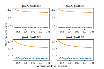
Figure 2: Prediction errors of the REDAR algorithm run on a randomly generated system are seen to fall below the error bound at all times.

It should be noted that the bound is clearly not tight on the system above. A tighter bound could be obtained by removing several of the cruder bounding techniques, and choosing free parameters in the bound more carefully. This effort was not undertaken in this this work.

VI Conclusion

The finite sample behavior of an algorithm known as REDAR was characterized for data generated in closed-loop. The algorithm follows an approach used by many identification methods in which the data is fit to a VARX model, and the system model is obtained via a reduction step. Due to the simple nature of the algorithm, it was possible to derive a non-asymptotic upper bound on the generalization error. Though the bound is not tight, it provides the engineer with a notion of the effectiveness of the model with a finite amount of data, which allows for comparison of algorithms and parameter selection for the model. Additionally, high probability bounds on the $\mathcal{H}_{\infty}$ norm of the error system from the estimated model to the finite horizon Kalman Filter are obtained. It may be possible to utilize these bounds for robust control synthesis. As the analysis holds for identification of closed loop systems, this would allow for an adaptive approach to robust control design to be applied.

VII Acknowledgements

The authors thank Jianjun Yuan for helpful discussions regarding the finite data bound.

References

• [1] L. Ljung, System identification: theory for the user, 2nd ed.   Prentice-hall, 1999.
• [2] M. Mohri, A. Rostamizadeh, and A. Talwalkar, Foundations of machine learning.   MIT press, 2018.
• [3] A. Goldenshluger, “Nonparametric estimation of transfer functions: rates of convergence and adaptation,” IEEE Transactions on Information Theory, vol. 44, no. 2, pp. 644–658, March 1998.
• [4] A. Goldenshluger, A. Zeevi et al., “Nonasymptotic bounds for autoregressive time series modeling,” The Annals of Statistics, vol. 29, no. 2, pp. 417–444, 2001.
• [5] S. Tu, R. Boczar, A. Packard, and B. Recht, “Non-asymptotic analysis of robust control from coarse-grained identification,” arXiv preprint arXiv:1707.04791, 2017.
• [6] M. Simchowitz, H. Mania, S. Tu, M. I. Jordan, and B. Recht, “Learning without mixing: Towards a sharp analysis of linear system identification,” arXiv preprint arXiv:1802.08334, 2018.
• [7] S. Oymak and N. Ozay, “Non-asymptotic identification of lti systems from a single trajectory,” arXiv preprint arXiv:1806.05722, 2018.
• [8] T. Sarkar, A. Rakhlin, and M. A. Dahleh, “Finite-Time System Identification for Partially Observed LTI Systems of Unknown Order,” arXiv e-prints, p. arXiv:1902.01848, Feb 2019.
• [9] E. Hazan, K. Singh, and C. Zhang, “Learning linear dynamical systems via spectral filtering,” in Advances in Neural Information Processing Systems, 2017, pp. 6702–6712.
• [10] E. Hazan, H. Lee, K. Singh, C. Zhang, and Y. Zhang, “Spectral filtering for general linear dynamical systems,” in Advances in Neural Information Processing Systems, 2018, pp. 4634–4643.
• [11] E. Hazan et al., “Introduction to online convex optimization,” Foundations and Trends® in Optimization, vol. 2, no. 3-4, pp. 157–325, 2016.
• [12] N. Cesa-Bianchi and G. Lugosi, Prediction, learning, and games.   Cambridge university press, 2006.
• [13] M. Gevers, “Identification for control: From the early achievements to the revival of experiment design,” European Journal of Control, vol. 11, pp. 12– 12, 01 2006.
• [14] S. Dean, H. Mania, N. Matni, B. Recht, and S. Tu, “On the Sample Complexity of the Linear Quadratic Regulator,” arXiv e-prints, p. arXiv:1710.01688, Oct 2017.
• [15] U. Forssell and L. Ljung, “Closed-loop identification revisited,” Automatica, vol. 35, no. 7, pp. 1215 – 1241, 1999.
• [16] L. Ljung and T. McKelvey, “Subspace identification from closed loop data,” Signal Processing, vol. 52, no. 2, pp. 209 – 215, 1996, subspace Methods, Part II: System Identification.
• [17] M. Jansson, “Subspace identification and arx modeling,” IFAC Proceedings Volumes, vol. 36, no. 16, pp. 1585 – 1590, 2003, 13th IFAC Symposium on System Identification (SYSID 2003), Rotterdam, The Netherlands, 27-29 August, 2003.
• [18] A. Chiuso, “The role of vector autoregressive modeling in predictor-based subspace identification,” Automatica, vol. 43, no. 6, pp. 1034–1048, 2007.
• [19] S. J. Qin, “An overview of subspace identification,” Computers and Chemical Engineering, vol. 30, no. 10, pp. 1502 – 1513, 2006, papers form Chemical Process Control VII.
• [20] G. van der Veen, J.-W. van Wingerden, M. Bergamasco, M. Lovera, and M. Verhaegen, “Closed-loop subspace identification methods: an overview,” IET Control Theory & Applications, vol. 7, no. 10, pp. 1339–1358, 2013.
• [21] A. Dahlen and W. Scherrer, “The relation of the cca subspace method to a balanced reduction of an autoregressive model,” Journal of Econometrics, vol. 118, no. 1-2, pp. 293–312, 2004.
• [22] K. Zhou, J. C. Doyle, K. Glover et al., Robust and optimal control.   Prentice hall New Jersey, 1996, vol. 40.
• [23] M. J. Wainwright, High-dimensional statistics: A non-asymptotic viewpoint.   Cambridge University Press, 2019, vol. 48.