Accelerated Information Gradient flow

Abstract.

We present a framework for Nesterov’s accelerated gradient flows in probability space to design efficient mean-field Markov chain Monte Carlo (MCMC) algorithms for Bayesian inverse problems. Here four examples of information metrics are considered, including Fisher-Rao metric, Wasserstein-2 metric, Kalman-Wasserstein metric and Stein metric. For both Fisher-Rao and Wasserstein-2 metrics, we prove convergence properties of accelerated gradient flows. In implementations, we propose a sampling-efficient discrete-time algorithm for Wasserstein-2, Kalman-Wasserstein and Stein accelerated gradient flows with a restart technique. We also formulate a kernel bandwidth selection method, which learns the gradient of logarithm of density from Brownian-motion samples. Numerical experiments, including Bayesian logistic regression and Bayesian neural network, show the strength of the proposed methods compared with state-of-the-art algorithms.

Keywords. Nesterov’s accelerated gradient method; Bayesian inverse problem; Optimal transport; Information geometry

1. Introduction

Optimization problems in probability space, arising from Bayesian inference Liu and Wang, (2016) and inverse problems Stuart, (2010), attract increasing attentions in machine learning communities Liu et al., (2018); Bernton, (2018); Wibisono, (2019). One typical example here is to draw samples from an intractable target distribution. Such sampling problem is important in providing exploration in distribution of interest and quantifying uncertainty among data. From an optimization viewpoint, this problem suffices to minimize an objective functional, such as Kullback-Leibler (KL) divergence, which is to measure the closeness between current density and the target distribution.

Gradient descent methods play essential roles in solving these optimization problems. Here the gradient direction relies on the information metric in probability space. In literature, two important metrics, such as Fisher-Rao metric and Wasserstein-2 (in short, Wasserstein) metric, are of great interests Lafferty, (1988); Amari, (1998); Otto, (2001). The information gradient direction in terms of density corresponds to the update rule in a set of samples. This is known as sampling formulation or particle implementation of gradient flow, which yields various sampling algorithms. For Fisher-Rao metric, its gradient flow relates to birth-death dynamics, which is important in model selection and modeling population games Amari, (2016). The Fisher-Rao gradient, also known as natural gradient, is also useful in designing fast and reliable algorithms in probability models Amari, (1998); Kingma and Ba, (2014); Malago et al., (2013); Martens and Grosse, (2015). For Wasserstein metric, the gradient flow of KL divergence is the Fokker-Planck equation of overdamped Langevin dynamic. In sampling algorithms, the time discretization of overdamped Langevin dynamics yields the classical Langevin Markov chain Monte Carlo (MCMC) method and the proximal Langevin algorithm Bernton, (2018); Wibisono, (2019). In recent years, various first-order sampling methods via generalized Wasserstein gradient direction are proposed. For example, the Stein variational gradient descent Liu and Wang, (2016) formulates kernelized interacting Langevin dynamics. The Kalman-Wasserstein gradient, also known as ensemble Kalman sampling Garbuno-Inigo et al., (2019), induces covariance-preconditioned mean-field interacting Langevin dyanmics.

For classical optimization problems in Euclidean space, the Nesterov’s accelerated gradient method Nesterov, (1983) is a wide-applied optimization method and it accelerates gradient descent methods. The continuous-time limit of this method is known as the accelerated gradient flow Su et al., (2016). Natural questions arise: What is the accelerated gradient flow in probability space under general information metrics? What is the corresponding discrete-time sampling algorithm? For optimization problems on a Riemannian manifold, accelerated gradient methods are studied in Liu et al., (2017); Zhang and Sra, (2018). The probability space embedded with information metric can be viewed as a Riemannian manifold, known as density manifold Lafferty, (1988). Several previous works explore accelerated methods in this manifold under Wasserstein metric. An acceleration framework of particle-based variational inference (ParVI) methods is proposed in Liu et al., (2018, 2019) based on manifold optimization. Taghvaei and Mehta Taghvaei and Mehta, (2019) introduce accelerated flows from an optimal control perspective. Similar dynamics has been studied from a fluid dynamics viewpoint Carrillo et al., 2019a . Underdamped Langevin dynamics is another way to accelerate on MCMC Cheng et al., (2017); Ma et al., (2019).

In this paper, we present a unified framework of accelerated gradient flows in probability space embedded with information metrics, named Accelerated Information Gradient (AIG) flows. From a transport-information-geometry perspective, we derive AIG flows by damping Hamiltonian flows. Examples include Fisher-Rao metric, Wasserstein-2 metric, Kalman-Wasserstein metric and Stein metric. In Gaussian families, we verify the existence of AIG flows. Here we show that the AIG flow corresponds to a well-posed ODE system in the space of symmetric positive definite matrices. We rigorously prove the convergence rate of AIG flows based on the geodesic convexity of the loss function under both Fisher-Rao metric and Wasserstein metric. Besides, we handle two difficulties in numerical implementations of AIG flows under Wasserstein metric for sampling. On the one hand, as pointed out in Liu et al., (2019); Taghvaei and Mehta, (2019), the logarithm of density term (gradient of KL divergence) is difficult to approximate in particle formulations. We propose a novel kernel selection method, whose bandwidth is learned by sampling from Brownian motions. We call it the BM method. On the other hand, we notice that the AIG flow can be a numerically stiff system, especially in high-dimensional sample spaces. This is because the solution of AIG flows can be close to the boundary of the probability space. To handle this issue, we propose an adaptive restart technique, which accelerates and stabilizes the discrete-time algorithm. Numerical results in Bayesian Logistic regression and Bayesian neural networks indicate the validity of the BM method and the acceleration effects of proposed AIG flows.

This paper is organized as follows. Section 2 briefly reviews gradient flows and accelerated gradient flows in Euclidean space. Then, the information metrics in probability space and their corresponding gradient and Hamiltonian flows are introduced. In Section 3, we formulate AIG flows, under Fisher-Rao metric, Wasserstein metric, Kalman-Wasserstein metric and Stein metric. We theoretically prove the convergence rate of AIG flows in Section 4. Section 5 presents the discrete-time algorithm for W-AIG flows, including the BM method and the adaptive restart technique. Section 6 provides numerical experiments. In supplementary materials, we also provide discrete-time algorithms for both Kalman-Wasserstein AIG and Stein AIG flows.

2. Reviews

In this section, we review gradient flows and accelerated gradient flows in Euclidean space. Then, we introduce the optimization problems in probability spaces, and review several definitions of information metrics therein. Based on these metrics, we demonstrate gradient and Hamiltonian flows in probability space. These formulations serve necessary preparations for us to derive accelerated gradient flows in probability space. See detailed analysis on metrics in probability space in Amari et al., (1987); Saha, (2019); Srivastava and Klassen, (2016).

2.1. Accelerated gradient flows in Euclidean space

Consider an optimization problem in Euclidean space:

$$\min_{x\in\mathbb{R}^{n}}f(x),$$

where $f(x)$ is a given convex function with $L$-Lipschitz continuous gradient. Here $\left\langle\cdot,\cdot\right\rangle$ and $\|\cdot\|$ are the Euclidean inner product and norm in $\mathbb{R}^{n}$. The gradient descent method has the update rule

$$x_{k+1}=x_{k}-\tau_{k}\nabla f(x_{k}),$$

where $\tau_{k}>0$ is a step size. With the limit $\tau_{k}\to 0$, the continuous-time limit of gradient descent method is the gradient flow (GF)

$$\dot{x}_{t}=-\nabla f(x_{t}).$$

To accelerate the gradient descent method, Nesterov introduced an accelerated method Nesterov, (1983):

$$\left\{\begin{aligned} &\mathbf{x}_{k}=\mathbf{y}_{k-1}-\tau_{k}\nabla f(\mathbf{y}_{k-1}),\\ &\mathbf{y}_{k}=\mathbf{x}_{k}+\alpha_{k}(\mathbf{x}_{k}-\mathbf{x}_{k-1}).\end{aligned}\right.$$

Here $\alpha_{k}$ depends on the convexity of $f(x)$. If $f(x)$ is $\beta$-strongly convex, then $\alpha_{k}=\frac{\sqrt{L}-\sqrt{\beta}}{\sqrt{L}+\sqrt{\beta}}$; otherwise, $\alpha_{k}=\frac{k-1}{k+2}$. Su et al., (2016) show that the continuous-time limit of Nesterov’s accelerated method satisfies an ODE, which is known as the accelerated gradient flow (AGF):

$$\ddot{x}_{t}+\alpha_{t}\dot{x}_{t}+\nabla f(x_{t})=0.$$ (1)

Here $\alpha_{t}=2\sqrt{\beta}$ if $f(x)$ is $\beta$-strongly convex; $\alpha_{t}=3/t$ for general convex $f(x)$.

An important observation in Maddison et al., (2018) is that the accelerated gradient flow (1) can be formulated as a damped Hamiltonian flow:

$$\begin{bmatrix}\dot{x}_{t}\\ \dot{p}_{t}\end{bmatrix}+\begin{bmatrix}0\\ \alpha_{t}p_{t}\end{bmatrix}-\begin{bmatrix}0&I\\ -I&0\end{bmatrix}\begin{bmatrix}\nabla_{x}H^{E}(x_{t},p_{t})\\ \nabla_{p}H^{E}(x_{t},p_{t})\end{bmatrix}=0.$$

where $x$ is the state variable and $p$ is the momentum variable. The Hamiltonian function satisfies $H^{E}(x,p)=\frac{\|p\|^{2}}{2}+f(x)$, which consists of Euclidean kinetic function $\frac{\|p\|^{2}}{2}$ and potential function $f(x)$. In other words, one can formulate an accelerated gradient flow by adding a linear momentum term into the Hamiltonian flow. Later on, we follow this damped Hamiltonian perspective and derive related accelerated gradient flows in probability space.

2.2. Metrics in probability space

In practice, machine learning problems, especially Bayesian sampling problems, can be formulated as optimization problems in probability space. In other words, consider

$$\min_{\rho\in\mathcal{P}(\Omega)}E(\rho),$$

where $\Omega\subset\mathbb{R}^{n}$ is a region and the set of probability density is denoted by $\mathcal{P}(\Omega)=\{\rho\in\mathcal{F}(\Omega)\colon\int_{\Omega}\rho dx=1,\quad\rho\geq 0\}$. Here $\mathcal{F}(\Omega)$ represents the set of smooth functions on $\Omega$. In practice, $E(\rho)$ is often chosen as a divergence or metric functional between $\rho$ and a target density $\rho^{*}\in\mathcal{P}(\Omega)$.

In literature, it has been shown that various sampling algorithms correspond to gradient flows of $E(\rho)$, depending on the metrics in probability space. We brief review the definition of metrics in probability space as follows.

Definition 1 (Metric in probability space).

Denote the tangent space at $\rho\in\mathcal{P}(\Omega)$ by $T_{\rho}\mathcal{P}(\Omega)=\left\{\sigma\in\mathcal{F}(\Omega):\int\sigma dx=0.\right\}$. The cotangent space at $\rho$, $T^{*}_{\rho}\mathcal{P}(\Omega)$, can be treated as the quotient space $\mathcal{F}(\Omega)/\mathbb{R}$.A metric tensor $G(\rho):T_{\rho}\mathcal{P}(\Omega)\to T^{*}_{\rho}\mathcal{P}(\Omega)$ is an invertible mapping from $T_{\rho}\mathcal{P}(\Omega)$ to $T_{\rho}^{*}\mathcal{P}(\Omega)$. This metric tensor defines the metric (inner product) on tangent space $T_{\rho}\mathcal{P}(\Omega)$:

$$g_{\rho}(\sigma_{1},\sigma_{2})=\int\sigma_{1}G(\rho)\sigma_{2}dx=\int\Phi_{1}G(\rho)^{-1}\Phi_{2}dx,\quad\sigma_{1},\sigma_{2}\in T_{\rho}\mathcal{P}(\Omega)$$

where $\Phi_{i}$ is the solution to $\sigma_{i}=G(\rho)^{-1}\Phi_{i}$, $i=1,2$.

Along with a given metric, the probability space $\mathcal{P}(\Omega)$ can be viewed as an infinite-dimensional Riemannian manifold, which is known as the density manifold Lafferty, (1988). We review four examples of metrics in $\mathcal{P}(\Omega)$: the Fisher-Rao metric from information geometry, the Wasserstein metric from optimal transport, the Kalman-Wasserstein metric from ensemble Kalman sampling and the Stein metric from Stein variational gradient method. For simplicity, we denote $\mathbb{E}_{\rho}[\Phi]=\int\Phi\rho dx$.

Example 1 (Fisher-Rao metric).

The inverse of Fisher-Rao metric tensor is defined by

$$G^{F}(\rho)^{-1}\Phi=\rho\left(\Phi-\mathbb{E}_{\rho}[\Phi]\right),\quad\Phi\in T_{\rho}^{*}\mathcal{P}(\Omega).$$

Example 2 (Wasserstein metric).

The inverse of Wasserstein metric tensor writes

$$G^{W}(\rho)^{-1}\Phi=-\nabla\cdot(\rho\nabla\Phi),\quad\Phi\in T_{\rho}^{*}\mathcal{P}(\Omega).$$

Example 3 (Kalman-Wasserstein metric, Garbuno-Inigo et al., (2019)).

The inverse of metric tensor is defined by

$$G^{KW}(\rho)^{-1}\Phi=-\nabla\cdot(\rho C^{\lambda}(\rho)\nabla\Phi),\quad\Phi\in T_{\rho}^{*}\mathcal{P}(\Omega).$$

Here $\lambda\geq 0$ is a given regularization constant and $C^{\lambda}(\rho)\in\mathbb{R}^{n\times n}$ follows

$$C^{\lambda}(\rho)=\int(x-m(\rho))(x-m(\rho))^{T}\rho dx+\lambda I,\quad m(\rho)=\int x\rho dx.$$

Example 4 (Stein metric, Liu, (2017); Duncan et al., (2019)).

The inverse of Stein metric tensor is defined by

$$G^{S}(\rho)^{-1}\Phi(x)=-\nabla_{x}\cdot\left(\rho(x)\int k(x,y)\rho(y)\nabla_{y}\Phi(y)dy\right).$$

Here $k(x,y)$ is a given positive kernel function.

2.3. Gradient flows and Hamiltonian flows in probability space

The gradient flow for $E(\rho)$ in $(\mathcal{P}(\Omega),g_{\rho})$ takes the form

$$\partial_{t}\rho_{t}=-G(\rho_{t})^{-1}\frac{\delta E}{\delta\rho_{t}}.$$

Here $\frac{\delta E}{\delta\rho_{t}}$ is the $L^{2}$ first variation w.r.t. $\rho_{t}$. For example, the Wasserstein gradient flow writes

$$\begin{split}\partial_{t}\rho_{t}=&-G^{W}(\rho_{t})^{-1}\frac{\delta E}{\delta\rho_{t}}=\nabla\cdot\left(\rho_{t}\nabla\frac{\delta E}{\delta\rho_{t}}\right).\end{split}$$

We then briefly review Hamiltonian flows in probability space. Given a metric $\mathcal{G}(\rho)$, denote the density function $\rho_{t}$ as a state variable while function $\Phi_{t}$ as a momentum variable. The Hamiltonian flow in probability space follows

$$\partial_{t}\begin{bmatrix}\rho_{t}\\ \Phi_{t}\end{bmatrix}-\begin{bmatrix}0&1\\ -1&0\end{bmatrix}\begin{bmatrix}\frac{\delta}{\delta\rho_{t}}\mathcal{H}(\rho_{t},\Phi_{t})\\ \frac{\delta}{\delta\Phi_{t}}\mathcal{H}(\rho_{t},\Phi_{t})\end{bmatrix}=0,$$ (2)

with respect to the Hamiltonian in density space by

$$\mathcal{H}(\rho_{t},\Phi_{t})=\frac{1}{2}\int\Phi_{t}G(\rho_{t})^{-1}\Phi_{t}dx+E(\rho_{t}).$$

Similar to the Euclidean Hamiltonian function, the Hamiltonian functional in density space consists of a kinetic energy $\frac{1}{2}\int\Phi G(\rho)^{-1}\Phi dx$ and a potential energy $E(\rho)$.

3. Accelerated information gradient flow

We introduce the accelerated gradient flow in probability density space as follows. Let $\alpha_{t}\geq 0$ be a scalar function of $t$. We add a damping term $\alpha_{t}\Phi_{t}$ to the Hamiltonian flow (2):

$$\partial_{t}\begin{bmatrix}\rho_{t}\\ \Phi_{t}\end{bmatrix}+\begin{bmatrix}0\\ \alpha_{t}\Phi_{t}\end{bmatrix}-\begin{bmatrix}0&1\\ -1&0\end{bmatrix}\begin{bmatrix}\frac{\delta}{\delta\rho_{t}}\mathcal{H}(\rho_{t},\Phi_{t})\\ \frac{\delta}{\delta\Phi_{t}}\mathcal{H}(\rho_{t},\Phi_{t})\end{bmatrix}=0.$$ (3)

We call dynamics (3) Accelerated Information Gradient (AIG) flow.

Proposition 1.

The accelerated information gradient flow satisfies

$$\left\{\begin{aligned} &\partial_{t}\rho_{t}-G(\rho_{t})^{-1}\Phi_{t}=0,\\ &\partial_{t}\Phi_{t}+\alpha_{t}\Phi_{t}+\frac{1}{2}\frac{\delta}{\delta\rho_{t}}\left(\int\Phi_{t}G(\rho_{t})^{-1}\Phi_{t}dx\right)+\frac{\delta E}{\delta\rho_{t}}=0,\\ \end{aligned}\right.$$ (AIG)

with initial values $\rho_{t}|_{t=0}=\rho_{0}$ and $\Phi_{t}|_{t=0}=0$.

We give examples of AIG flows under several metrics, such as Fisher-Rao metric, Wasserstein metric, Kalman-Wasserstein metric and Stein metric. See detailed derivations in the supplementary material.

Example 5 (Fisher-Rao AIG flow).

$$\left\{\begin{aligned} &\partial_{t}\rho_{t}-\left(\Phi_{t}-\mathbb{E}_{\rho_{t}}[\Phi_{t}]\right)\rho_{t}=0,\\ &\partial_{t}\Phi_{t}+\alpha_{t}\Phi_{t}+\frac{1}{2}\Phi_{t}^{2}-\mathbb{E}_{\rho_{t}}[\Phi_{t}]\Phi_{t}+\frac{\delta E}{\delta\rho_{t}}=0.\end{aligned}\right.$$ (F-AIG)

Example 6 (Wasserstein AIG flow, Carrillo et al., 2019a ; Taghvaei and Mehta, (2019)).

$$\left\{\begin{aligned} &\partial_{t}\rho_{t}+\nabla\cdot(\rho_{t}\nabla\Phi_{t})=0,\\ &\partial_{t}\Phi_{t}+\alpha_{t}\Phi_{t}+\frac{1}{2}\|\nabla\Phi_{t}\|^{2}+\frac{\delta E}{\delta\rho_{t}}=0.\\ \end{aligned}\right.$$ (W-AIG)

Example 7 (Kalman-Wasserstein AIG flow).

$$\left\{\begin{aligned} &\partial_{t}\rho_{t}+\nabla\cdot(\rho_{t}C^{\lambda}(\rho_{t})\nabla\Phi_{t})=0,\\ &\partial_{t}\Phi_{t}+\alpha_{t}\Phi_{t}+\frac{1}{2}\Big{(}(x-m(\rho_{t}))^{T}B_{\rho_{t}}(\Phi_{t})(x-m(\rho_{t}))\\ &+\nabla\Phi_{t}(x)^{T}C^{\lambda}(\rho_{t})\nabla\Phi_{t}(x)\Big{)}+\frac{\delta E}{\delta\rho_{t}}=0.\\ \end{aligned}\right.$$ (KW-AIG)

Here we denote $B_{\rho}(\Phi)=\int\nabla\Phi\nabla\Phi^{T}\rho dx$.

Example 8 (Stein AIG flow).

$$\left\{\begin{aligned} &\partial_{t}\rho_{t}(x)+\nabla_{x}\cdot\left(\rho_{t}(x)\int k(x,y)\rho_{t}(y)\nabla_{y}\Phi_{t}(y)dy\right)=0,\\ &\partial_{t}\Phi_{t}(x)+\alpha_{t}\Phi_{t}(x)+\int\nabla\Phi_{t}(x)^{T}\nabla\Phi_{t}(y)k(x,y)\rho_{t}(y)dy+\frac{\delta E}{\delta\rho_{t}}(x)=0.\end{aligned}\right.$$ (S-AIG)

To design fast sampling algorithms, we need to reformulate the evolution of probability in term of samples. In other words, PDEs in term of $(\rho,\Phi)$ is the Eulerian formulation in fluid dynamics, while the particle formulation is the flow map equation, known as the Lagrangian formulation. We present examples for W-AIG flow, KW-AIG flow and S-AIG flow, which have particle formulations. We suppose that $X_{t}\sim\rho_{t}$ and $V_{t}=\nabla\Phi_{t}(X_{t})$ are the position and the velocity of a particle at time $t$.

Example 9 (Particle W-AIG flow).

The particle dynamical system for the flow (W-AIG) writes

$$\left\{\begin{aligned} &\frac{d}{dt}X_{t}=V_{t},\\ &\frac{d}{dt}V_{t}=-\alpha_{t}V_{t}-\nabla\left(\frac{\delta E}{\delta\rho_{t}}\right)(X_{t}).\end{aligned}\right.$$ (4)

Example 10 (Particle KW-AIG flow).

The particle dynamical system for the flow (KW-AIG) writes

$$\left\{\begin{aligned} &\frac{dX_{t}}{dt}=C^{\lambda}(\rho_{t})V_{t},\\ &\frac{dV_{t}}{dt}=-\alpha_{t}V_{t}-\mathbb{E}[V_{t}V_{t}^{T}](X_{t}-\mathbb{E}[X_{t}])-\nabla\left(\frac{\delta E}{\delta\rho_{t}}\right)(X_{t}).\end{aligned}\right.$$ (5)

Here the expectation is taken over the particle system.

Example 11 (Particle S-AIG flow).

The particle dynamical system for the flow (S-AIG) writes

$$\left\{\begin{aligned} &\frac{dX_{t}}{dt}=\int k(X_{t},y)\nabla\Phi_{t}(y)\rho_{t}(y)dy,\\ &\frac{dV_{t}}{dt}=-\alpha_{t}V_{t}-\int V_{t}^{T}\nabla\Phi_{t}(y)\nabla_{x}k(X_{t},y)\rho_{t}(y)dy-\nabla\left(\frac{\delta E}{\delta\rho_{t}}\right)(X_{t}).\end{aligned}\right.$$ (6)

We notice that dynamics in examples 9 to 11 are mean-field dynamics. Here the mean-field represents that the dynamics evolves its own probability density function in its path. In addition, they are also mean field Markov process. Here the Markov property holds in the sense that the update of dynamics only depends on the current time probability density. Shortly, we will design a finite dimensional particle dynamical system to simulate these proposed dynamics.

In later on algorithm and convergence analysis, the choice of $\alpha_{t}$ is important. Similar as the ones in Euclidean space, $\alpha_{t}$ depends on the convexity of $E(\rho)$ w.r.t. given metrics.

Definition 2 (Convexity in probability space).

For a functional $E(\rho)$ defined on the probability space, we say that $E(\rho)$ is $\beta$-strongly convex w.r.t. metric $g_{\rho}$ if there exists a constant $\beta\geq 0$ such that for any $\rho\in\mathcal{P}(\Omega)$ and any $\sigma\in T_{\rho}\mathcal{P}(\Omega)$, we have

$$g_{\rho}(\operatorname{Hess}E(\rho)\sigma,\sigma)\geq\beta g_{\rho}(\sigma,\sigma).$$

Here $\operatorname{Hess}$ is the Hessian operator w.r.t. $g_{\rho}$. If $\beta=0$, we say that $E(\rho)$ is convex w.r.t. metric $g_{\rho}$.

Again, if $E(\rho)$ is $\beta$-strongly convex for $\beta>0$, then $\alpha_{t}=2\sqrt{\beta}$; if $E(\rho)$ is convex, then $\alpha_{t}=3/t$.

We can also formulate W-AIG flows in probability models. For instance, the W-AIG flow in Gaussian families becomes an ODE system, which corresponds to updates of covariance matrices.

Proposition 2 (W-AIG flows in Gaussian families).

Suppose that $\rho_{0},\rho^{*}$ are Gaussian distributions with zero means and their covariance matrices are $\Sigma_{0}$ and $\Sigma^{*}$. $E(\Sigma)$ evaluates the KL divergence from $\rho$ to $\rho^{*}$:

$$E(\Sigma)=\frac{1}{2}\left[\operatorname{tr}(\Sigma(\Sigma^{*})^{-1})-\log\det(\Sigma(\Sigma^{*})^{-1})-n\right],$$ (7)

Let $(\Sigma_{t},S_{t})$ be the solution to

$$\left\{\begin{aligned} &\dot{\Sigma}_{t}-2(S_{t}\Sigma_{t}+\Sigma_{t}S_{t})=0,\\ &\dot{S}_{t}+\alpha_{t}S_{t}+2S_{t}^{2}+\nabla_{\Sigma_{t}}E(\Sigma_{t})=0,\end{aligned}\right.$$ (W-AIG-G)

with initial values $\Sigma_{t}|_{t=0}=\Sigma_{0}$ and $S_{t}|_{t=0}=0$. Here $\Sigma_{t}$ and $S_{t}$ are symmetric matrices. Then, for any $t\geq 0$, $\Sigma_{t}$ is well-defined and stays positive definite. Furthermore, we denote

$$\rho_{t}(x)=\frac{(2\pi)^{-n/2}}{\sqrt{\det(\Sigma_{t})}}\exp\left(-\frac{1}{2}x^{T}\Sigma_{t}^{-1}x\right),\quad\Phi_{t}(x)=x^{T}S_{t}x+C(t),$$

where $C(t)=-t+\frac{1}{2}\int_{0}^{t}\log\det(\Sigma_{s}(\Sigma^{*})^{-1})ds.$ Then, $(\rho_{t},\Phi_{t})$ is the solution to (W-AIG) with initial values $\rho_{t}|_{t=0}=\rho_{0}$ and $\Phi_{t}|_{t=0}=0$.

Remark 1.

If the means of $\rho_{0},\rho^{*}$ are $\mu_{0}$ and $\mu^{*}$ instead of $0$, the objective function turns to be

$$E(\Sigma,\mu)= \frac{1}{2}[\operatorname{tr}(\Sigma(\Sigma^{*})^{-1})-\log\det(\Sigma(\Sigma^{*})^{-1})-n]$$

$$+\frac{1}{2}(\mu-\mu^{*})^{T}(\Sigma^{*})^{-1}(\mu-\mu^{*})].$$

It is separable in terms of $\mu$ and $\sigma$. For simplicity and clarity, we focus on the case with zero means.

Remark 2.

AIG flows can be formulated into general probability models, such as Gaussian mixture models and generative models. We leave the systematic study of AIG flows in models in future works.

4. Convergence rate analysis on AIG flows

In this section, we prove the convergence rates of AIG flows under either the Wasserstein metric or the Fisher-Rao metric. This validates the acceleration effect. The proof is motivated by Lyapunov functions of Euclidean accelerated gradient flows in subsection 2.1.

Theorem 1.

Suppose that $E(\rho)$ is $\beta$-strongly convex for $\beta>0$. The solution $\rho_{t}$ to (F-AIG) or (W-AIG) with $\alpha_{t}=2\sqrt{\beta}$ satisfies

$$E(\rho_{t})\leq C_{0}e^{-\sqrt{\beta}t}=\mathcal{O}\left(e^{-\sqrt{\beta}t}\right).$$

If $E(\rho)$ is convex, then the solution $\rho_{t}$ to (F-AIG) or (W-AIG) with $\alpha_{t}=3/t$ satisfies

$$E(\rho_{t})\leq C_{0}^{\prime}t^{-2}=\mathcal{O}(t^{-2}).$$

Here the constants $C_{0},C_{0}^{\prime}$ only depend on $\rho_{0}$.

Remark 3.

For $\beta$-strongly convex $E(\rho)$ under the Wasserstein metric, Carrillo et al., 2019a study a compressed Euler equation. They prove similar results with a constant damping coefficient $\alpha_{t}$. For convex $E(\rho)$ under the Wasserstein metric, Taghvaei and Mehta, (2019) prove similar results with a technical assumption.

Remark 4.

Compared to underdamped Langevin dynamics, W-AIG has the accelerated convergence rate guarantee compared to W-GF and it has a closer relation with the Euclidean accelerated gradient flow.

Remark 5.

The Fisher metric and the Wasserstein metric are two popular metrics to consider in the probability space. Therefore, we focus on deriving the convergence analysis for these two metrics. The convergence results for other general information metrics are interesting problems for future studies.

In Euclidean case, the convergence rate of accelerated gradient flow is based on the construction of Lyapunov functions. Namely, for $\beta$-strongly convex $f(x)$, consider a Lyapunov function:

$$\mathcal{E}(t)=\frac{e^{\sqrt{\beta}t}}{2}\|\sqrt{\beta}(x_{t}-x^{*})+\dot{x}_{t}\|^{2}+e^{\sqrt{\beta}t}(f(x_{t})-f(x^{*})).$$

For general convex $f(x)$, consider a Lyapunov function

$$\mathcal{E}(t)=\frac{1}{2}\left\|(x_{t}-x^{*})+\frac{t}{2}\dot{x}_{t}\right\|^{2}+\frac{t^{2}}{4}(f(x_{t})-f(x^{*})).$$

Based on different assumptions on the convexity of $f(x)$, we can prove that these Lyapunov function are not increasing w.r.t. $t$. Hence, the convergence rates are obtained.

Remark 6.

Our choices of the damping parameter $\alpha_{t}$ are analogous to these in the Euclidean case. In the Euclidean case, the damped Hamiltonian system and the related Lyapunov functions are derived from the Bregman Lagrangian introduced in Wibisono et al., (2016); Wilson et al., (2016). For simplicity, we only focus on two specific choices of the damping parameters $\alpha_{t}$, based on the convexity of the energy functional.

Following Lyapunov functions in Euclidean space, we provide a sketch of the proof for Theorem 1. We first consider the case where $E(\rho)$ is $\beta$-strongly convex for $\beta>0$. Let $T_{t}$ denote the optimal transport plan from $\rho_{t}$ to $\rho^{*}$. Consider a Lyapunov function

$$\mathcal{E}(t)= \frac{e^{\sqrt{\beta}t}}{2}\int\left\|-\sqrt{\beta}(T_{t}(x)-x)+\nabla\Phi_{t}(x)\right\|^{2}\rho_{t}(x)dx$$ (8)

$$+e^{\sqrt{\beta}t}(E(\rho_{t})-E(\rho^{*})).$$

Here the $-(T_{t}(x)-x)$ term can be viewed as $x_{t}-x^{*}$ and $\nabla\Phi_{t}$ can be viewed as $\dot{x}_{t}$. Different from the Euclidean case, we introduce an important lemma in proving that $\mathcal{E}(t)$ is non-increasing.

Lemma 1.

Denote $u_{t}=\partial_{t}(T_{t})^{-1}\circ T_{t}$. Then,$u_{t}$ satisfies

$$\nabla\cdot\left(\rho_{t}(u_{t}-\nabla\Phi_{t})\right)=0.$$

We also have

$$\partial_{t}T_{t}(x)=-\nabla T_{t}(x)u_{t}(x).$$

More importantly, we have

$$\int\left\langle\nabla\Phi_{t}-u_{t},\nabla T_{t}\nabla\Phi_{t}\right\rangle\rho_{t}dx\geq 0,$$

$$\int\left\langle\nabla\Phi_{t}-u_{t},\nabla T_{t}(x)(T_{t}(x)-x)\right\rangle\rho_{t}=0.$$

We then demonstrate that $\mathcal{E}(t)$ is not increasing w.r.t. $t$.

Proposition 3.

Suppose that $E(\rho)$ satisfies Hess($\beta$) for $\beta>0$. $\rho_{t}$ is the solution to (W-AIG) with $\alpha_{t}=2\sqrt{\beta}$. Then, $\mathcal{E}(t)$ defined in (8) satisfies $\dot{\mathcal{E}}(t)\leq 0.$ As a result,

$$E(\rho_{t})\leq e^{-\sqrt{\beta}t}\mathcal{E}(t)\leq e^{-\sqrt{\beta}t}\mathcal{E}(0)=\mathcal{O}(e^{-\sqrt{\beta}t}).$$

Note that $\mathcal{E}(0)$ only depends on $\rho_{0}$. This proves the first part of Theorem 1.

We now focus on the case where $E(\rho)$ is convex. Similarly, we construct the following Lyapunov function.

$$\mathcal{E}(t)= \frac{1}{2}\int\left\|-(T_{t}(x)-x)+\frac{t}{2}\nabla\Phi_{t}(x)\right\|^{2}\rho_{t}(x)dx$$ (9)

$$+ \frac{t^{2}}{4}(E(\rho_{t})-E(\rho^{*})).$$

Proposition 4.

Suppose that $E(\rho)$ satisfies Hess($0$). $\rho_{t}$ is the solution to (W-AIG) with $\alpha_{t}=3/t$. Then, $\mathcal{E}(t)$ defined in (9) satisfies $\dot{\mathcal{E}}(t)\leq 0.$ As a result,

$$E(\rho_{t})\leq\frac{4}{t^{2}}\mathcal{E}(t)\leq\frac{4}{t^{2}}\mathcal{E}(0)=\mathcal{O}(t^{-2}).$$

Because $\mathcal{E}(0)$ only depends on $\rho_{0}$, we complete the proof.

5. Discrete-time algorithms for AIG flows

In this section, we present the discrete-time particle implementation of the flow (W-AIG) based on the particle W-AIG flow (4). Similar discrete-time algorithms of (KW-AIG) and (S-AIG) are provided in the supplementary material. Here we mainly introduce a kernel bandwidth selection method and an adaptive restart technique to deal with difficulties in numerical implementations.

A typical choice of $E(\rho)$ for sampling is the KL divergence

$$\mathrm{D}_{\textrm{KL}}(\rho\|\rho^{*})=\int\rho\log\frac{\rho}{e^{-f}}dx-\log Z,$$

where the target density $\rho^{*}(x)\propto\exp(-f(x))$ and $Z=\int\exp(-f(x))dx$. Then, (4) is equivalent to

$$\left\{\begin{aligned} &dX_{t}=V_{t}dt,\\ &dV_{t}=-\alpha_{t}V_{t}dt-\nabla f(X_{t})dt-\nabla\log\rho_{t}(X_{t})dt.\end{aligned}\right.$$ (10)

Consider a particle system $\{X_{0}^{i}\}_{i=1}^{N}$ and let $V_{0}^{i}=0$. In $k$-th iteration, the update rule follows

$$\left\{\begin{aligned} &X_{k+1}^{i}=X_{k}^{i}+\sqrt{\tau_{k}}V_{k+1}^{i},\\ &V_{k+1}^{i}=\alpha_{k}V_{k}^{i}-\sqrt{\tau_{k}}(\nabla f(X_{k}^{i})+\xi_{k}(X_{k}^{i})),\\ \end{aligned}\right.$$ (11)

for $i=1,2\dots N$. If $E(\rho)$ is $\beta$-strongly convex, then $\alpha_{k}=\frac{1-\sqrt{\beta\tau_{k}}}{1+\sqrt{\beta\tau_{k}}}$; if $E(\rho)$ is convex or $\beta$ is unknown, then $\alpha_{k}=\frac{k-1}{k+2}$. Here $\xi_{k}(x)$ is an approximation of $\nabla\log\rho_{k}(x)$. For a general distribution, we use the kernel density estimation (KDE) Singh, (1977), $\tilde{\rho}_{k}(x)=\frac{1}{N}\sum_{i=1}^{N}K(x,X_{k}^{i})$ to approximate $\rho_{k}(x)$. Here $K(x,y)$ is a positive kernel function. Then, $\xi_{k}$ writes

$$\xi_{k}(x)=\nabla\log\tilde{\rho}_{k}(x)=\frac{\sum_{i=1}^{N}\nabla_{x}K(x,X_{k}^{i})}{\sum_{i=1}^{N}K(x,X_{k}^{i})}.$$ (12)

A common choice of $K(x,y)$ is a Gaussian kernel with the bandwidth $h$, $K(x,y)=(2\pi h)^{-n/2}\exp\left(-\|x-y\|^{2}/(2h)\right)$. Such approximation can also be found in information-theoretic learning Principe et al., (2000) and independent component analysis (ICA) Deco and Obradovic, (2012).

There are two difficulties in the time discretization. For one thing, the bandwidth $h$ strongly affects the estimation of $\nabla\log\rho_{t}$, so we propose the BM method to learn the bandwidth from Brownian-motion samples. For another, the second equation in (W-AIG) is the Hamilton-Jacobi equation, which usually has strong stiffness. In numerical trials, we observe that the densities from the particles may collapse in certain dimensions following W-AIG flows, even for Gaussian target density. Therefore, we propose an adaptive restart technique to deal with this problem.

Remark 7.

Using symplectic integrators for the particle implementation of W-AIG could help improve the performance. It is important to study the time-discretization of the (damped) Hamiltonian flow in the future.

5.1. Learn the bandwidth via Brownian motion

SVGD uses a median (MED) method to choose the bandwidth, i.e.,

$$h_{k}=\frac{1}{2\log(N+1)}\text{median}\left(\{\|X_{k}^{i}-X_{k}^{j}\|^{2}\}_{i,j=1}^{N}\right).$$ (13)

Liu et al. Liu et al., (2018) propose a Heat Equation (HE) method to adaptively adjust bandwidth. Motivated by the HE method, we introduce the Brownian motion (BM) method to adaptively learn the kernel bandwidth based on Brownian-motion samples generated in each iteration.

Given the bandwidth $h$, $\{X_{k}^{i}\}_{i=1}^{N}$ and a step size $s$, we can compute two particle systems:

$$Y_{k}^{i}(h)=X_{k}^{i}-s\xi_{k}(x;h),\quad Z_{k}^{i}=X_{k}^{i}+\sqrt{2s}B^{i},\quad i=1,\dots N$$

where $B^{i}$ is the standard Brownian motion. Denote the empirical distributions of $\{X_{k}^{i}\}_{i=1}^{N}$, $\{Y_{k}^{i}\}_{i=1}^{N}$ and $\{Z_{k}^{i}\}_{i=1}^{N}$ by $\hat{\rho}_{X},\hat{\rho}_{Y}$ and $\hat{\rho}_{Z}$. With $n\to\infty$, we shall have $\hat{\rho}_{Y}=\hat{\rho}_{Z}=\rho_{t}|_{t=s}$, where $\hat{\rho}_{t}$ satisfies $\partial_{t}\hat{\rho}_{t}=\Delta\hat{\rho}_{t}=\nabla\cdot(\hat{\rho}_{t}\nabla\log\hat{\rho}_{t})$ with initial value $\hat{\rho}_{t}|_{t=0}=\hat{\rho}_{X}$. With an appropriate bandwidth $h$, we shall also have $\hat{\rho}_{Y}=\rho_{t}|_{t=s}$. Hence, we consider the following optimization problem

$$\min_{h}\operatorname{MMD}(\hat{\rho}_{Y},\hat{\rho}_{Z})=\int\int(\hat{\rho}_{Y}(y)-\hat{\rho}_{Z}(y))k(y,z)(\hat{\rho}_{Y}(z)-\hat{\rho}_{Z}(z))dydz.$$ (14)

where MMD (maximum mean discrepancy) evaluates the similarity between $\{Y_{k}^{i}\}_{i=1}^{N}$ and $\{Z_{k}^{i}\}_{i=1}^{N}$. Here, the kernel $k(y,z)$ in MMD is chosen as a Gaussian kernel with bandwidth $1$. So we optimize (14) using the bandwidth $h_{k-1}$ from the last iteration as the initialization. For simplicity we denote

$$\text{BM}(h_{k-1},\{X_{k}^{i}\}_{i=1}^{N},s)$$

as the minimizer of problem (14). It is the output of the BM method.

Remark 8.

Besides KDE, there are other methods that approximate the term $\nabla\log\rho_{t}(x)$ (compute $\xi_{k}$) via a kernel function, such as the blob method Carrillo et al., 2019b and the diffusion map Taghvaei and Mehta, (2019). The BM method can also select the kernel bandwidth for these methods.

5.2. Adaptive restart

To enhance the practical performance, we introduce an adaptive restart technique, which shares the same idea of gradient restart in O’donoghue and Candes, (2015); Wang et al., 2019b under the Euclidean case. Consider

$$\varphi_{k}=-\sum_{i=1}^{N}\left\langle V_{k+1}^{i},\nabla f(X_{k}^{i})+\xi_{k}(X_{k}^{i})\right\rangle,$$ (15)

which can be viewed as discrete-time approximation of

$$-g_{\rho_{t}}^{W}(\partial_{t}\rho_{t},G^{W}(\rho_{t})^{-1}\frac{\delta E}{\delta\rho_{t}})=-\partial_{t}E(\rho_{t}).$$

If $\varphi_{k}<0$, then we restart the algorithm with initial values $X_{0}^{i}=X_{k}^{i}$ and $V_{0}^{i}=0$. This essentially keeps $\partial_{t}E(\rho_{t})$ negative along the trajectory. The overall algorithm is summarized below.

Algorithm 1 Discrete-time particle implementation of W-AIG flow

0:  initial positions $\{X_{0}^{i}\}_{i=1}^{N}$, step size $\tau$, number of iteration $L$.

1:  Set $k=0$, $V_{0}^{i}=0,i=1,\dots N$. Set the bandwidth $h_{0}$ by MED (13).

2:  for $l=1,2,\dots L$ do

3:     Compute $h_{l}$ based on BM method: $h_{l}=\text{BM}(h_{l-1},\{X_{k}^{i}\}_{i=1}^{N},\sqrt{\tau})$.

4:     Calculate $\xi_{k}(X_{k}^{i})$ by (12) with bandwidth $h_{l}$.

5:     For $i=1,2,\dots N$, update $V_{k+1}^{i}$ and $X_{k+1}^{i}$ by (11).

6:     Compute $\varphi_{k}$ by (15).

7:     If $\varphi_{k}<0$, set $X_{0}^{i}=X_{k}^{i}$ and $V_{0}^{i}=0$ and $k=0$; otherwise set $k=k+1$.

8:  end for

6. Numerical experiments

In this section, we present several numerical experiments to demonstrate the effectiveness of BM method, the acceleration effect of AIG flows, and the strength of adaptive restart technique. Implementation details are provided in the supplementary material.

6.1. Toy examples

We first generate samples from a toy bi-modal distribution in (Rezende and Mohamed,, 2015). We compare sampling algorithms based on gradient flows and accelerated gradient flows under Wasserstein metric, Kalman-Wasserstein metric and Stein metric. The number of particles follow $N=200$. The initial distribution of the particle system follows $\mathcal{N}([0,10]^{\prime},I)$.

For the approximation of $\nabla\log\rho_{k}$, we use a Gaussian kernel and the kernel bandwidth is selected by the BM method. We apply the restart technique for discrete-time algorithms of AIG flows. For W-GF, W-AIG, SVGD and S-AIG, we take the step size $\tau_{k}=0.1$. For KW-GF and KW-AIG, we set the regularization parameter $\lambda=1$ and the step size $\tau_{k}=0.02$. We choose a smaller step size for the Kalman-Wasserstein metric because the particle system may blow up for a larger step size. For SVGD and S-AIG, we use a Gaussian kernel with fixed bandwidth $1$. The step size of SVGD is adjusted by Adagrad.

From Figure 1, the convergence rate of the particle system depends on the metric. For a fixed metric, samples generated by accelerated gradient flows always converge faster than the ones generated by gradient flows.

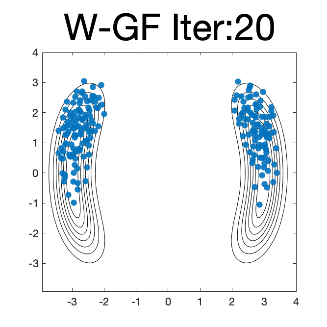
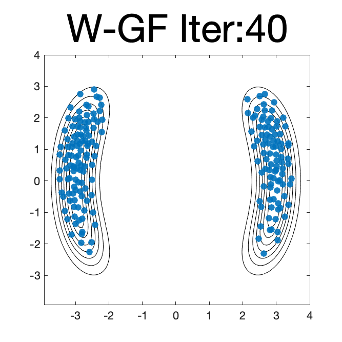
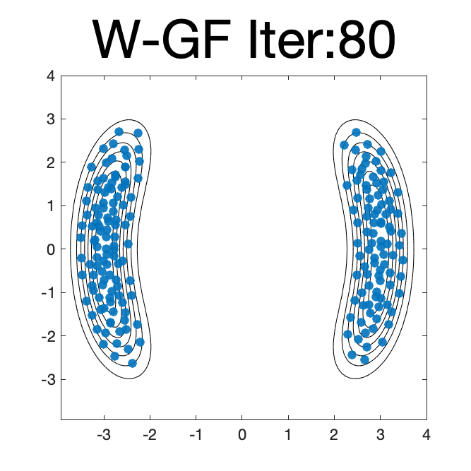
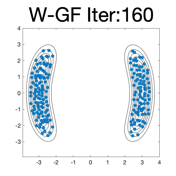
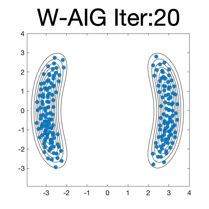
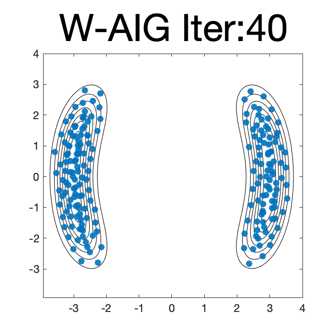
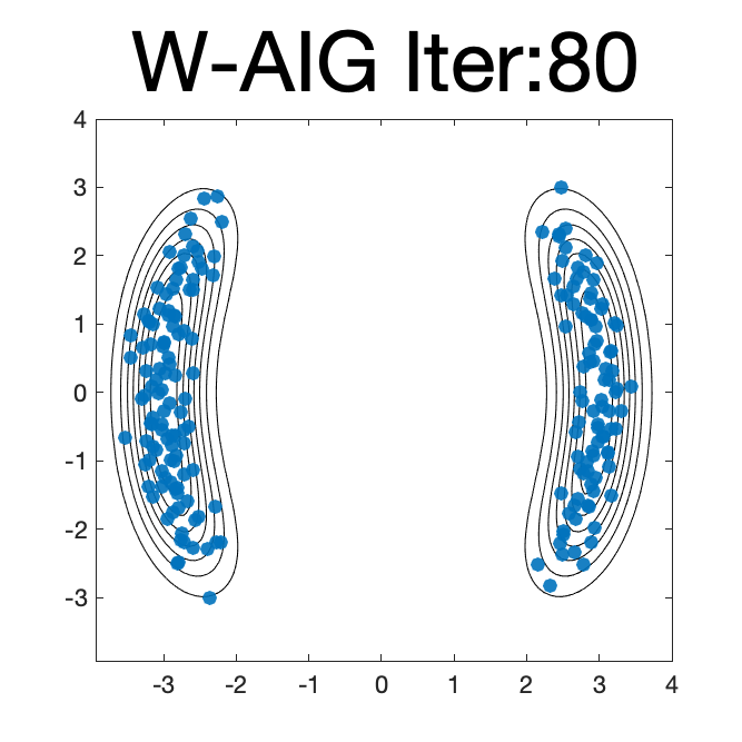
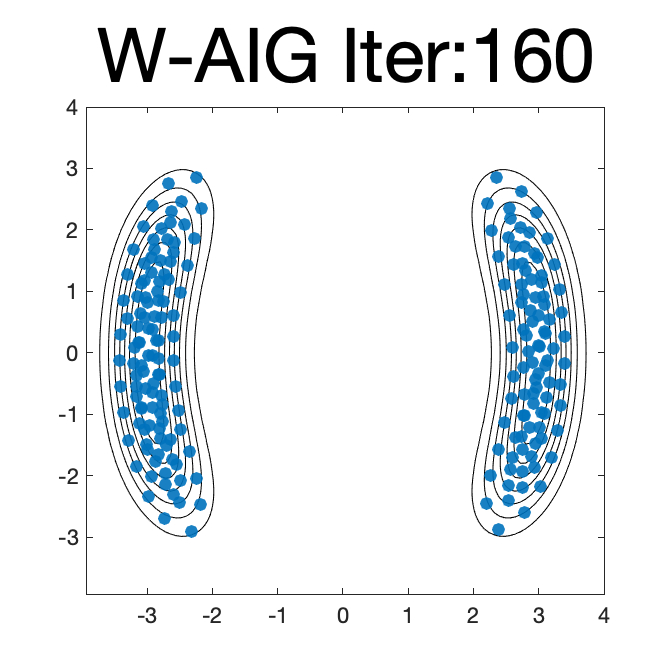
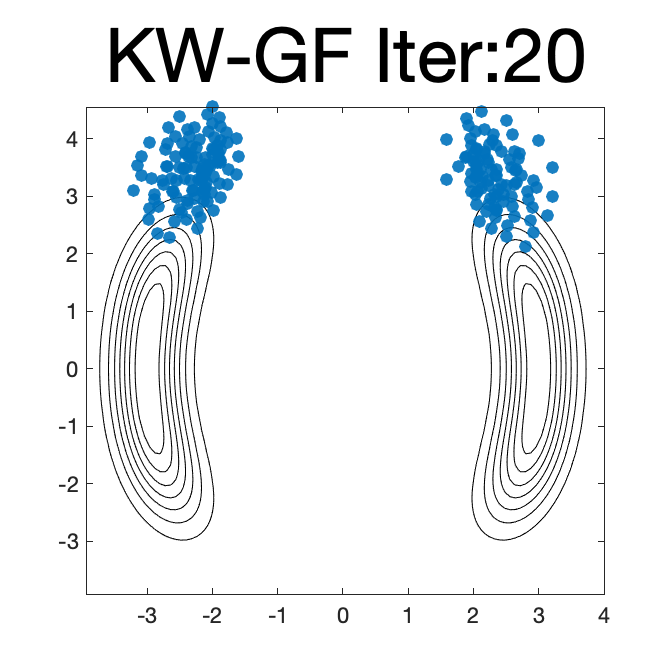
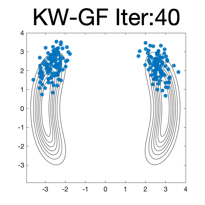
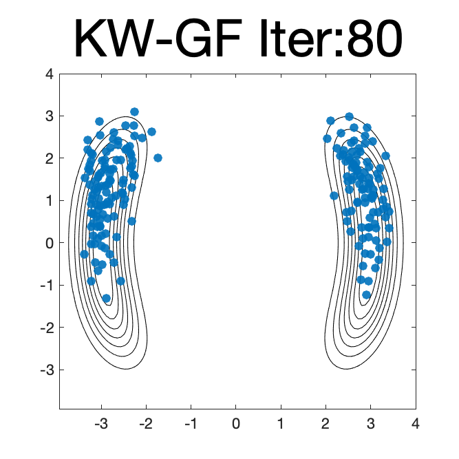
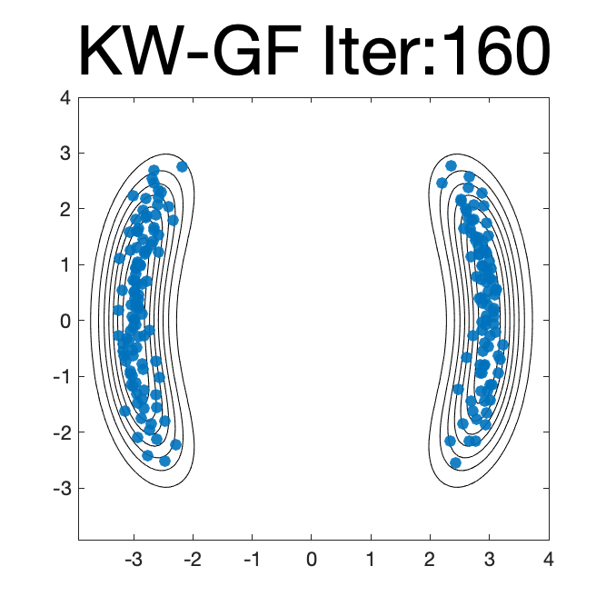
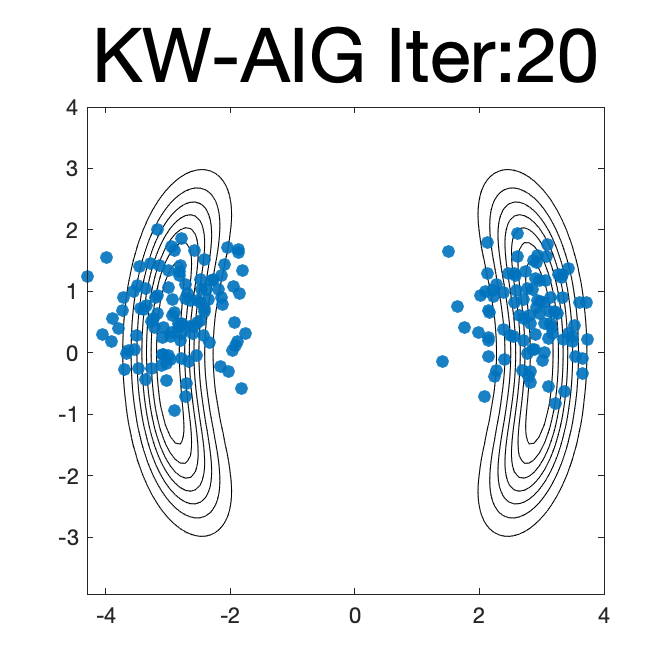
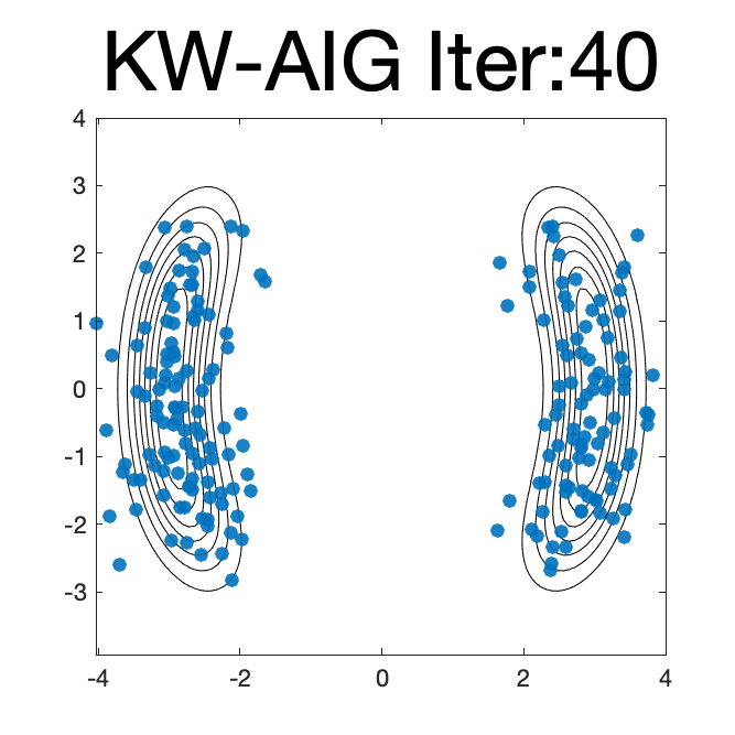
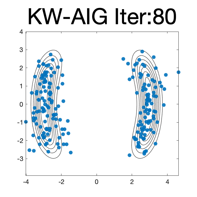
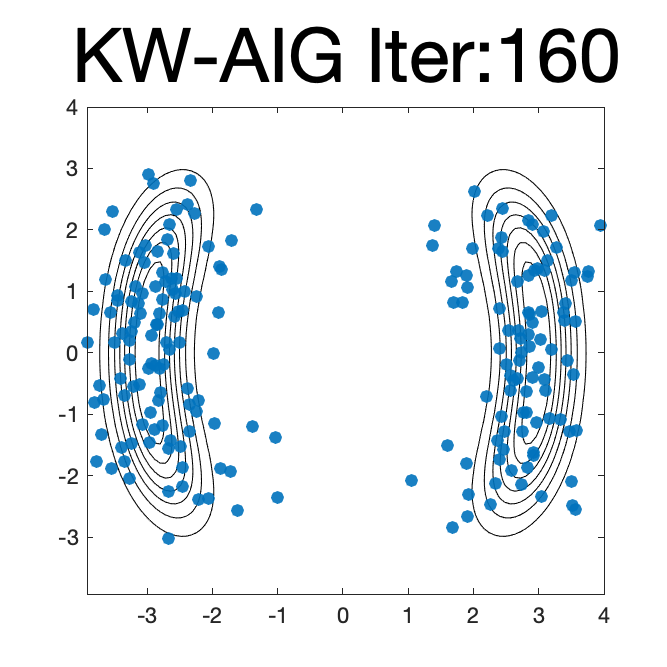
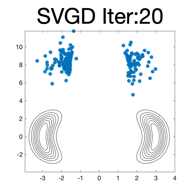
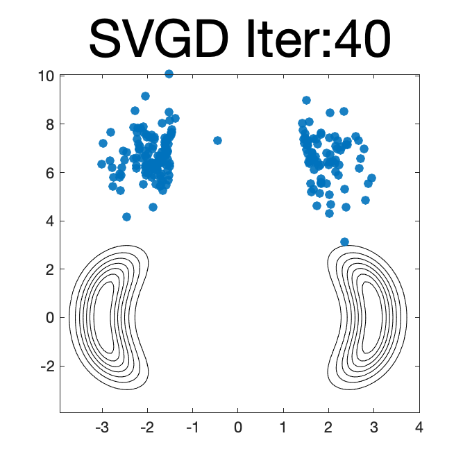
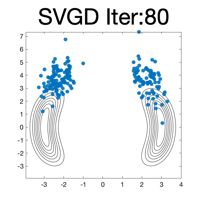
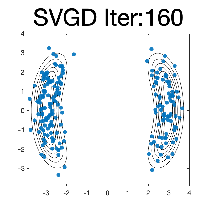
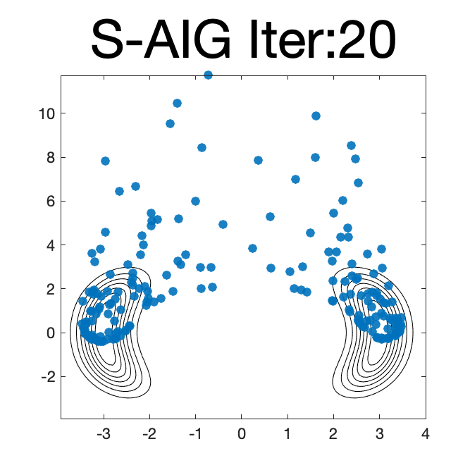
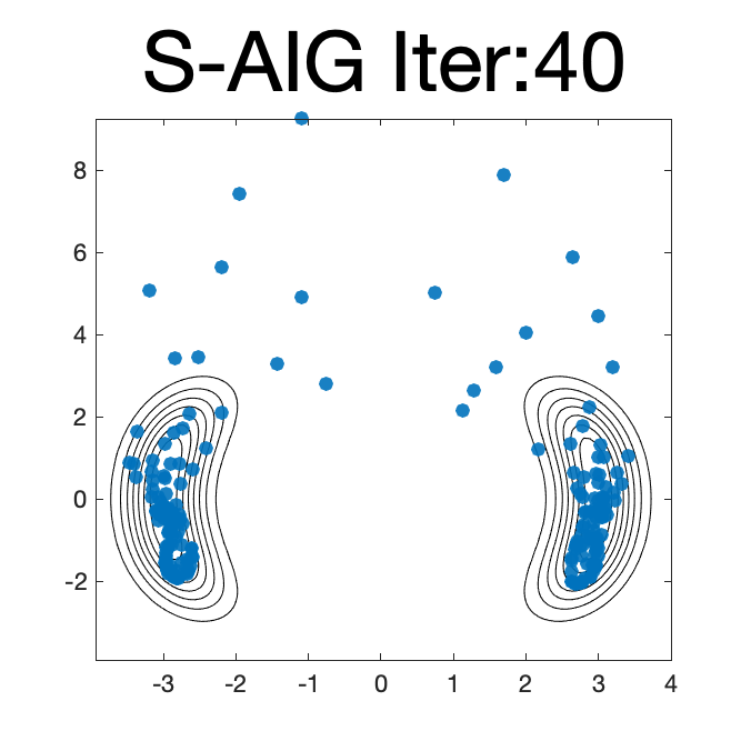
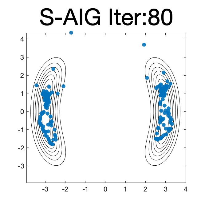
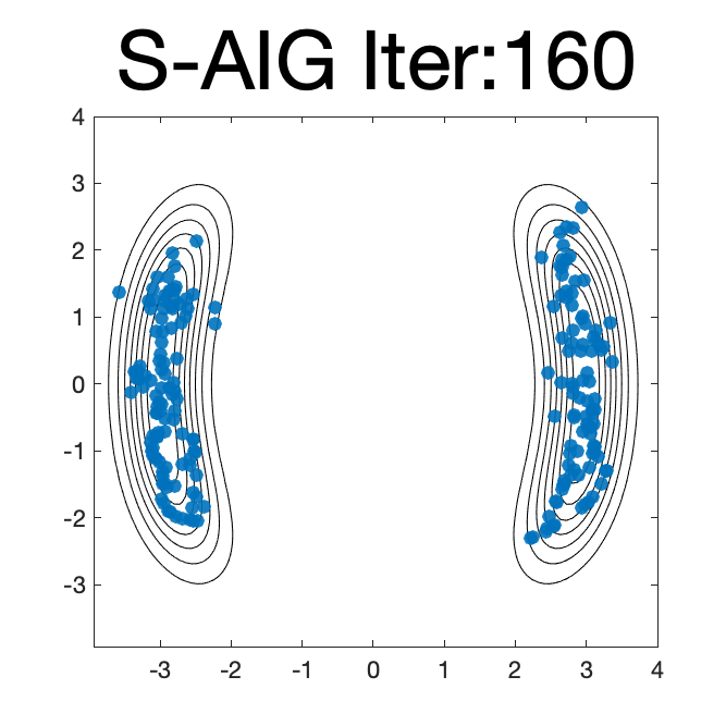
Figure 1. Comparison of different AIG flows on a toy example.

6.2. Effect of BM method

We first investigate the validity of the BM method in selecting the bandwidth. The target density $\rho^{*}$ is a toy bi-modal distribution (Rezende and Mohamed,, 2015). We compare two types of particle implementations of the Wasserstein gradient flow over KL divergence:

$$X_{k+1}^{i}=X_{k}^{i}-\tau\nabla f(X_{k}^{i})+\sqrt{2\tau}B_{k}^{i},$$

$$X_{k+1}^{i}=X_{k}^{i}-\tau(\nabla f(X_{k}^{i})+\xi_{k}(X_{k}^{i})).$$

Here $B_{k}^{i}\sim\mathcal{N}(0,1)$ is the standard Brownian motion and $\xi_{k}$ is estimated via KDE. The first method is known as the Langevin MCMC method and the second method is called the ParVI method. For ParVI methods, the bandwidth $h$ is selected by MED/HE/BM respectively. The initial distribution of the particle system follows the standard Gaussian $\mathcal{N}(0,I)$. The objective density function follows

$$\rho^{*}(x)\propto \exp(-2(\|x\|-3)^{2})$$

$$\times(\exp(-2(x_{1}-3)^{2})+\exp(-2(x_{1}+3)^{2})).$$

All methods run for $200$ iterations using the same fixed step size $\tau=0.1$.

Figure 1 shows the distribution of $200$ samples based on different methods. Samples from MCMC match the target distribution in a stochastic way; samples from MED collapse; samples from HE align tidily around contour lines; samples from BM arrange neatly and are closer to samples from MCMC. This indicates that the BM method makes the particle system behave similar to MCMC, though in a deterministic way.

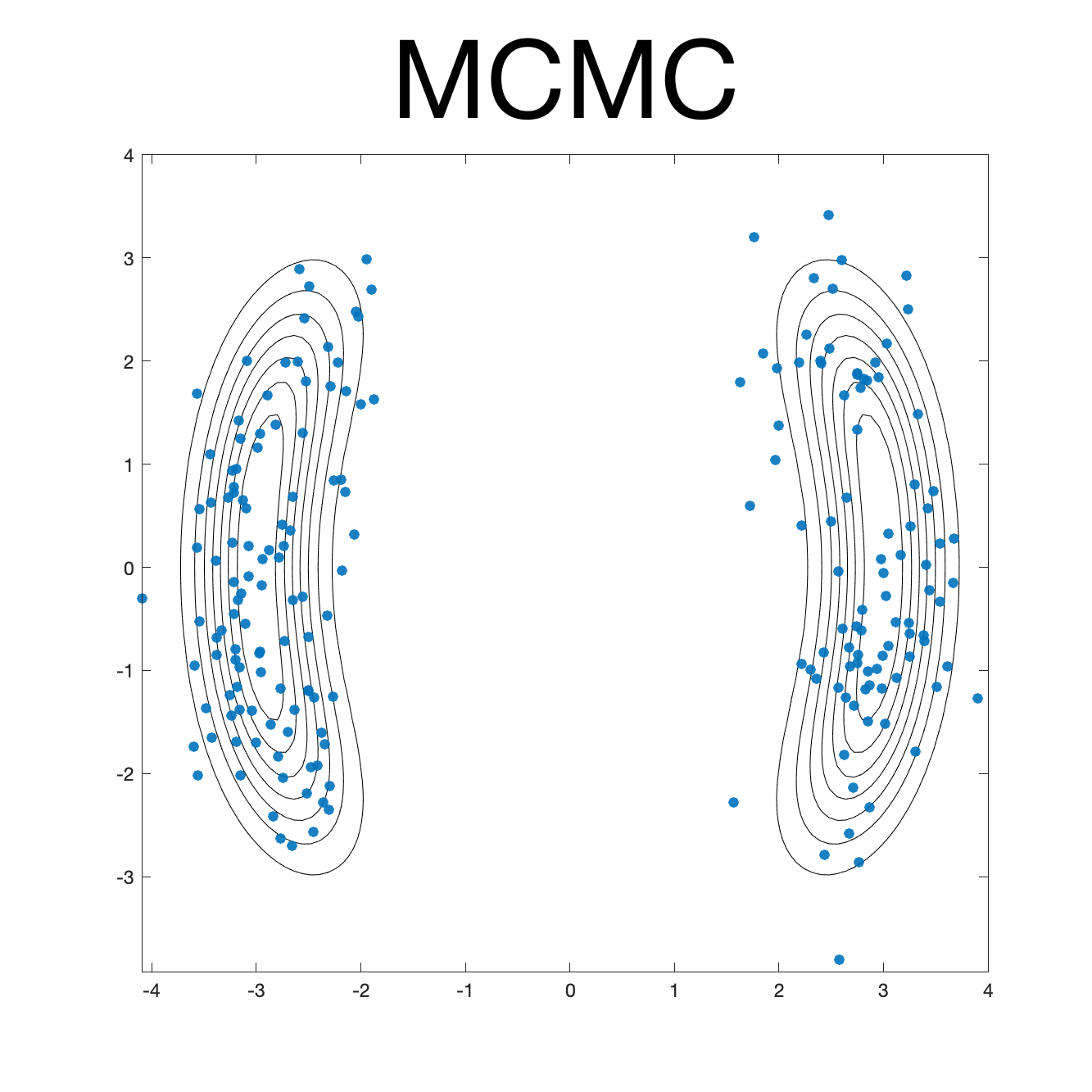
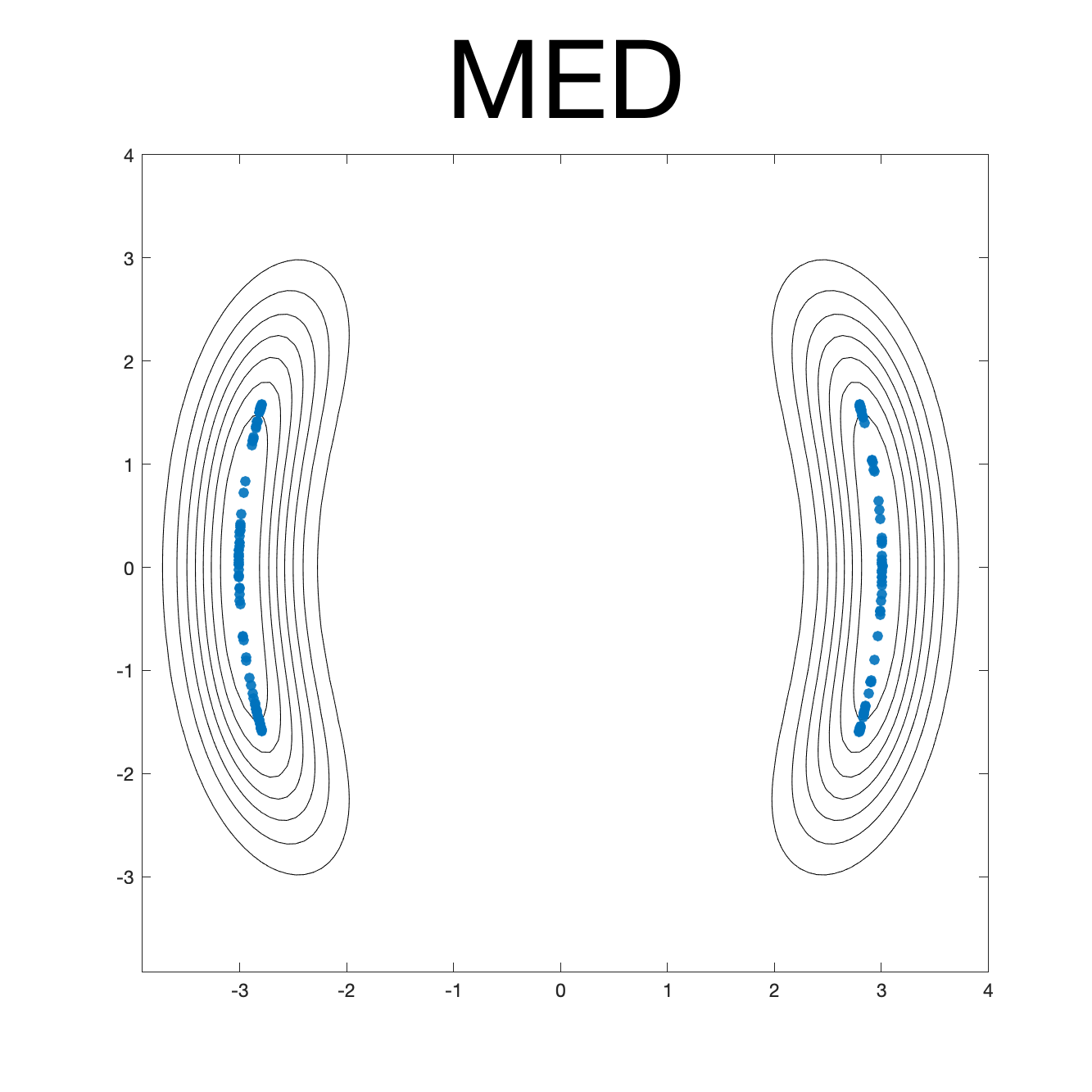
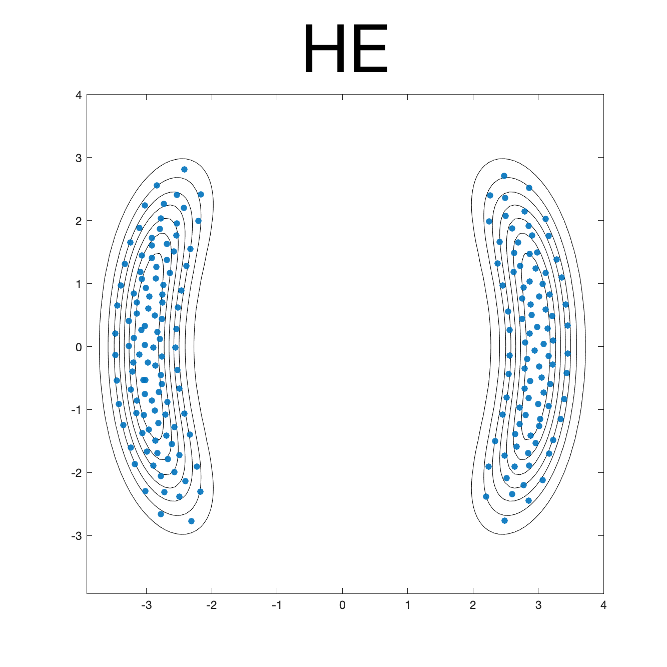
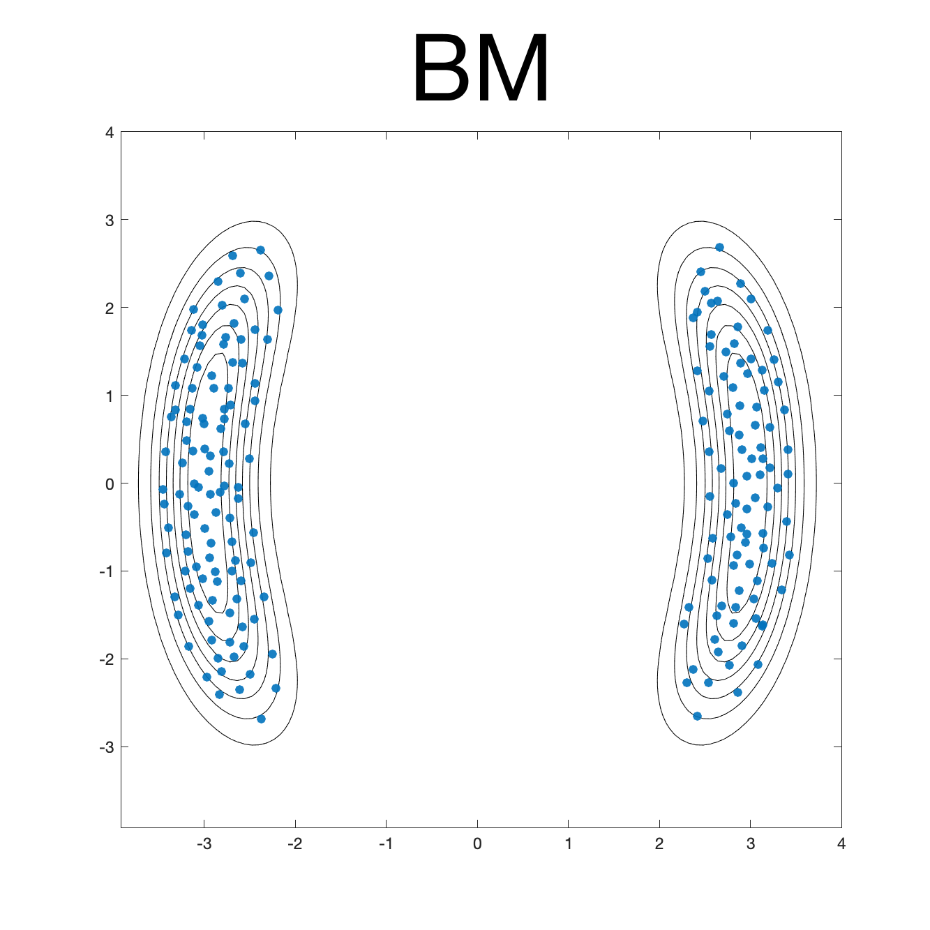
Figure 2. The effect of the BM method. Samples are plotted as blue dots. Left to right: MCMC, MED, HE and BM. All methods are run for $200$ iterations with the same initialization.

6.3. Bayesian logistic regression

We perform the standard Bayesian logistic regression experiment on the Covertype dataset, following the same settings as Liu and Wang, (2016). Our methods are compared with MCMC, SVGD Liu and Wang, (2016), WNAG Liu et al., (2018) and WNes Liu et al., (2019). SVGD is a gradient descent method based on the Stein metric, which approximates W-GF, see (Liu et al.,, 2019, Theorem 2). WNAG and WNes are two accelerated methods based on W-GF.

We select the kernel bandwidth using either the MED method or the proposed BM method. Figure 3 indicates that the BM method accelerates and stabilizes the performance of GFs and AIGs. The performance of MCMC and WGF are similar and they achieve the best log-likelihood. For a given metric, AIG flows have better test accuracy and test log-likelihood in first 2000 iterations. W-AIG and KW-AIG achieve $75\%$ test accuracy in less than 500 iterations.

Figure 3. Results on Bayesian logistic regression, averaged over $10$ independent trials. The shaded areas show the variance. Top: BM; Bottom: MED. Left: Test accuracy; Right: Test log-likelihood.

6.4. Bayesian neural network

We apply our proposed method on Bayesian neural network over the UCI datasets, with the same setting as Wang et al., 2019a . We compare W-AIG, W-GF and SVGD. For all methods, we use $N=10$ particles. The averaged results over $20$ independent trials are collected in Table 1 and 2. We observe that on most datasets, W-AIG has better test root-mean-square-error and test log-likelihood than W-GF and SVGD. This indicates that W-AIG may have better generalization than W-GF and SVGD.

Dataset	AIG	WGF	SVGD
Boston	$2.871_{\pm 3.41e-3}$	$3.077_{\pm 5.52e-3}$	$\mathbf{2.775_{\pm 3.78e-3}}$
Combined	$\mathbf{4.067_{\pm 9.27e-1}}$	$4.077_{\pm 3.85e-4}$	$4.070_{\pm 2.02e-4}$
Concrete	$\mathbf{4.440_{\pm 1.34e-1}}$	$4.883_{\pm 1.93e-1}$	$4.888_{\pm 1.39e-1}$
Kin8nm	$\mathbf{0.094_{\pm 5.56e-6}}$	$0.096_{\pm 3.36e-5}$	$0.095_{\pm 1.32e-5}$
Wine	$0.606_{\pm 1.40e-5}$	$0.614_{\pm 3.48e-4}$	$\mathbf{0.604_{\pm 9.89e-5}}$
Year	$8.876_{\pm 3.71e-4}$	$\mathbf{8.872_{\pm 2.81e-4}}$	$8.873_{\pm 7.19e-4}$

Table 1. Test root-mean-square-error (RMSE).

Dataset	AIG	WGF	SVGD
Boston	$\mathbf{-2.609_{\pm 1.34e-4}}$	$-2.694_{\pm 2.83e-4}$	$-2.611_{\pm 1.36e-4}$
Combined	$\mathbf{-2.822_{\pm 5.72e-3}}$	$-2.825_{\pm 2.36e-5}$	$-2.823_{\pm 1.24e-5}$
Concrete	$\mathbf{-2.884_{\pm 8.84e-3}}$	$-2.971_{\pm 8.93e-3}$	$-2.978_{\pm 6.05e-3}$
Kin8nm	$\mathbf{0.951_{\pm 6.43e-4}}$	$0.923_{\pm 3.37e-3}$	$0.932_{\pm 1.43e-3}$
Wine	$-0.961_{\pm 1.28e-4}$	$-0.961_{\pm 3.17e-4}$	$\mathbf{-0.952_{\pm 9.89e-5}}$
Year	$-3.654_{\pm 1.00e-5}$	$-3.655_{\pm 7.82e-6}$	$\mathbf{-3.652_{\pm 1.28e-5}}$

Table 2. Test log-likelihood.

7. Conclusion

In summary, we propose the framework of AIG flows by damping Hamiltonian flows with respect to certain information metrics in probability space.In theory, we establish the convergence rate of F-AIG and W-AIG flows. In algorithm, we propose particle formulations for W-AIG flow, KW-AIG and S-AIG flows. Numerically, we propose discrete-time algorithms and an adaptive restart technique to overcome numerical stiffness of AIG flows. To efficiently approximate $\nabla\log\rho_{k}(x)$, we introduce a novel kernel selection method by learning from Brownian-motion samples. Numerical experiments verify the acceleration effect of AIG flows and the strength of adaptive restart.

In future works, we intend to systematically explain the stiffness of AIG flows and effects of adaptive restart. We shall apply our results to general information metrics, especially for generalized Wasserstein metrics. We expect to study the related sampling efficient optimization methods and discrete-time algorithms. We also plan to incorporate Hessian operators in probability space Wang and Li, (2020) in designing higher-order accelerated algorithms. We shall compare these information metrics induced methods in terms of both computational complexity and sampling efficiency. We expect that the proposed accelerated algorithms will be useful in scientific computing of Bayesian inverse problems.

In this appendix, we formulate detailed derivations of examples and proofs of propositions. We also design particle implementations of KW-AIG flows, S-AIG flows and provide detailed implementations of experiments.

Appendix A Euler-Lagrange equation, Hamiltonian flows and AIG flows

In this section, we review and derive Euler-Lagrange equation, Hamiltonian flows and Euler-Lagrange formulation of AIG flows in probability space.

A.1. Derivation of the Euler-Lagrange equation

In this subsection, we derive the Euler-Lagrange equation in probability space. For a given metric $g_{\rho}$ in probability space, we can define a Lagrangian by

$$\mathcal{L}(\rho_{t},\partial_{t}\rho_{t})=\frac{1}{2}g_{\rho_{t}}(\partial_{t}\rho_{t},\partial_{t}\rho_{t})-E(\rho_{t}).$$

Proposition 5.

The Euler-Lagrange equation for this Lagrangian follows

$$\partial_{t}\left(\frac{\delta\mathcal{L}}{\delta(\partial_{t}\rho_{t})}\right)=\frac{\delta\mathcal{L}}{\delta\rho_{t}}+C(t),$$

where $C(t)$ is a spatially-constant function.

Proof.

For a fixed $T>0$ and two given densities $\rho_{0},\rho_{T}$, consider the variational problem

$$I(\rho_{t})=\inf\limits_{\rho_{t}}\left\{\left.\int_{0}^{T}\mathcal{L}(\rho_{t},\partial_{t}\rho_{t})dt\right|\rho_{t}|_{t=0}=\rho_{0},\rho_{t}|_{t=T}=\rho_{T}\right\}.$$

Let $h_{t}\in\mathcal{F}(\Omega)$ be the smooth perturbation function that satisfies $\int h_{t}dx=0,t\in\left[0,T\right]$ and $h_{t}|_{t=0}=h_{t}|_{t=T}\equiv 0$. Denote $\rho_{t}^{\epsilon}=\rho_{t}+\epsilon h_{t}$. Note that we have the Taylor expansion

$$I(\rho_{t}^{\epsilon})= \int_{0}^{T}\mathcal{L}(\rho_{t},\partial_{t}\rho_{t})dt$$

$$+\epsilon\int_{0}^{T}\int\left(\frac{\delta\mathcal{L}}{\delta\rho_{t}}h_{t}+\frac{\delta\mathcal{L}}{\delta(\partial_{t}\rho_{t})}\partial_{t}h_{t}\right)dxdt+o(\epsilon).$$

From $\left.\frac{dI(\rho_{t}^{\epsilon})}{d\epsilon}\right|_{\epsilon=0}=0$, it follows that

$$\int_{0}^{T}\int\left(\frac{\delta\mathcal{L}}{\delta\rho_{t}}h_{t}+\frac{\delta\mathcal{L}}{\delta(\partial_{t}\rho_{t})}\partial_{t}h_{t}\right)dxdt=0.$$

Note that $h_{t}|_{t=0}=h_{t}|_{t=T}\equiv 0$. Perform integration by parts w.r.t. $t$ yields

$$\int_{0}^{T}\int\left(\frac{\delta\mathcal{L}}{\delta\rho_{t}}-\partial_{t}\frac{\delta\mathcal{L}}{\delta(\partial_{t}\rho_{t})}\right)h_{t}dxdt=0.$$

Because $\int h_{t}dx=0$, the Euler-Lagrange equation holds with a spatially constant function $C(t)$. ∎

A.2. Derivation of Hamiltonian flow

In this subsection, we derive the Hamiltonian flow in the probability space. Denote $\Phi_{t}=\delta L/\delta(\partial_{t}\rho_{t})=G(\rho_{t})\partial_{t}\rho_{t}$. Then, the Euler-Lagrange equation can be formulated as a system of $(\rho_{t},\Phi_{t})$, i.e.,

$$\left\{\begin{aligned} &\partial_{t}\rho_{t}-G(\rho_{t})^{-1}\Phi_{t}=0,\\ &\partial_{t}\Phi_{t}+\frac{1}{2}\frac{\delta}{\delta\rho_{t}}\left(\int\Phi_{t}G(\rho_{t})^{-1}\Phi_{t}dx\right)+\frac{\delta E}{\delta\rho_{t}}=0.\end{aligned}\right.$$

First, we give a useful identity. Given a metric tensor $G(\rho):T_{\rho}\mathcal{P}(\Omega)\to T_{\rho}^{*}\mathcal{P}(\Omega)$, we have

$$\int\sigma_{1}G(\rho)\sigma_{2}dx=\int G(\rho)\sigma_{1}\sigma_{2}dx$$ (16)

$$= \int\Phi_{1}G(\rho)^{-1}\Phi_{2}dx=\int G(\rho)^{-1}\Phi_{1}\Phi_{2}dx.$$

Here $\Phi_{1}=G(\rho)^{-1}\sigma_{1}$ and $\Phi_{2}=G(\rho)^{-1}\sigma_{2}$. We then check that

$$\frac{\delta}{\delta\rho_{t}}\left(\int\partial_{t}\rho_{t}G(\rho_{t})\partial_{t}\rho_{t}dx\right)=-\frac{\delta}{\delta\rho_{t}}\left(\int\Phi_{t}G(\rho_{t})^{-1}\Phi_{t}dx\right).$$ (17)

Let $\tilde{\rho}_{t}=\rho_{t}+\epsilon h$, where $h\in T_{\rho_{t}}\mathcal{P}(\Omega)$. For all $\sigma\in T_{\rho_{t}}\mathcal{P}$, it follows

$$G(\rho_{t}+\epsilon h)^{-1}G(\rho_{t}+\epsilon h)\sigma=\sigma.$$

The first-order derivative w.r.t. $\epsilon$ of the left hand side shall be $0$, i.e.,

$$\left(\frac{\partial G(\rho_{t})^{-1}}{\partial\rho_{t}}\cdot h\right)G(\rho_{t})\sigma+G(\rho_{t})^{-1}\left(\frac{\partial G(\rho_{t})}{\partial\rho_{t}}\cdot h\right)\sigma=0.$$

Because $\partial_{t}\rho_{t}=G(\rho)^{-1}\Phi_{t}$, applying (16) yields

$$\int\partial_{t}\rho_{t}\left(\frac{\partial G(\rho_{t})}{\partial\rho_{t}}\cdot h\right)\partial_{t}\rho_{t}dx=\int\Phi_{t}G(\rho_{t})^{-1}\left(\frac{\partial G(\rho_{t})}{\partial\rho_{t}}\cdot h\right)\partial_{t}\rho_{t}dx$$ (18)

$$= -\int\Phi_{t}\left(\frac{\partial G(\rho_{t})^{-1}}{\partial\rho_{t}}\cdot h\right)G(\rho_{t})\partial_{t}\rho_{t}dx=-\int\Phi_{t}\left(\frac{\partial G(\rho_{t})^{-1}}{\partial\rho_{t}}\cdot h\right)\Phi_{t}dx.$$

Based on basic calculations, we can compute that

$$\int\partial_{t}\rho_{t}G(\tilde{\rho}_{t})\partial_{t}\rho_{t}dx-\int\partial_{t}\rho_{t}G(\rho_{t})\partial_{t}\rho_{t}dx=\epsilon\int\partial_{t}\rho_{t}\left(\frac{\partial G(\rho_{t})}{\partial\rho_{t}}\cdot h\right)\partial_{t}\rho_{t}dx+o(\epsilon),$$ (19)

$$-\int\Phi_{t}G(\tilde{\rho}_{t})^{-1}\Phi_{t}dx+\int\Phi_{t}G(\rho_{t})^{-1}\Phi_{t}dx=-\epsilon\int\Phi_{t}\left(\frac{\partial G(\rho_{t})^{-1}}{\partial\rho_{t}}\cdot h\right)\Phi_{t}dx+o(\epsilon).$$ (20)

Combining (18), (19) and (20) yields (17). Hence, the Euler-Lagrange equation is equivalent to

$$\partial_{t}\Phi_{t}=\frac{1}{2}\frac{\delta}{\delta\rho_{t}}\left(\int\partial_{t}\rho_{t}G(\rho_{t})\partial_{t}\rho_{t}dx\right)-\frac{\delta E}{\delta\rho_{t}}=-\frac{1}{2}\frac{\delta}{\delta\rho_{t}}\left(\int\Phi_{t}G(\rho_{t})^{-1}\Phi_{t}dx\right)-\frac{\delta E}{\delta\rho_{t}}.$$

This equation combining with $\partial_{t}\rho_{t}=G(\rho)^{-1}\Phi_{t}$ recovers the Hamiltonian flow. In short, the Euler-Lagrange equation is from the primal coordinates $(\rho_{t},\partial_{t}\rho_{t})$ and the Hamiltonian flow is from the dual coordinates $(\rho_{t},\Phi_{t})$. Similar interpretations can be found in (Chow et al.,, 2019).

A.3. The Euler-Lagrangian formulation of AIG flows

We can formulate the AIG flow as a second-order equation of $\rho_{t}$,

$$\frac{D^{2}}{Dt^{2}}\rho_{t}+\alpha_{t}\partial_{t}\rho_{t}+G(\rho_{t})^{-1}\frac{\delta E}{\delta\rho_{t}}=0.$$

Here $D^{2}/Dt^{2}$ is the covariant derivative w.r.t. metric $G(\rho)$. We can also explicitly write $\frac{D^{2}}{Dt^{2}}\rho_{t}$ as

$$\frac{D^{2}}{Dt^{2}}\rho_{t}= \partial_{tt}\rho_{t}-(\partial_{t}G(\rho_{t})^{-1})\partial_{t}\rho_{t}+\frac{1}{2}G(\rho_{t})^{-1}\frac{\delta}{\delta\rho_{t}}\left(\int\partial_{t}\rho_{t}G(\rho_{t})\partial_{t}\rho_{t}dx\right).$$

Appendix B Derivation of examples in Section 3

In this section, we present examples of gradient flows, Hamiltonian flows and derive particle dynamics examples in Section 3.

B.1. Examples of gradient flows

We first present several examples of gradient flows w.r.t. different metrics.

Example 12 (Fisher-Rao gradient flow).

$$\begin{split}\partial_{t}\rho_{t}=&-G^{F}(\rho_{t})^{-1}\frac{\delta E}{\delta\rho_{t}}=-\rho_{t}\left(\frac{\delta E}{\delta\rho_{t}}-\int\frac{\delta E}{\delta\rho_{t}}\rho_{t}dy\right).\end{split}$$

Example 13 (Wasserstein gradient flow).

$$\begin{split}\partial_{t}\rho_{t}=&-G^{W}(\rho_{t})^{-1}\frac{\delta E}{\delta\rho_{t}}=\nabla\cdot\left(\rho_{t}\nabla\frac{\delta E}{\delta\rho_{t}}\right).\end{split}$$

Example 14 (Kalman-Wasserstein gradient flow).

$$\begin{split}\partial_{t}\rho_{t}=&-G^{KW}(\rho_{t})^{-1}\frac{\delta E}{\delta\rho_{t}}=\nabla\cdot\left(\rho_{t}C^{\lambda}(\rho_{t})\nabla\left(\frac{\delta E}{\delta\rho_{t}}\right)\right).\end{split}$$

Example 15 (Stein gradient flow).

$$\begin{split}\partial_{t}\rho_{t}=&-G^{S}(\rho_{t})^{-1}\frac{\delta E}{\delta\rho_{t}}=\nabla_{x}\cdot\left(\rho_{t}(x)\int k(x,y)\rho_{t}(y)\nabla_{y}\left(\frac{\delta E}{\delta\rho_{t}}\right)dy\right).\end{split}$$

B.2. Examples of Hamiltonian flows

We next present several examples of Hamiltonian flows w.r.t. different metrics. The derivations simply follow from the definition of the given information metric and the formulations given in Appendix A.2.

Example 16 (Fisher-Rao Hamiltonian flow).

The Fisher-Rao Hamiltonian flow follows

$$\left\{\begin{aligned} &\partial_{t}\rho_{t}-\rho_{t}\left(\Phi_{t}-\mathbb{E}_{\rho_{t}}[\Phi_{t}]\right)=0,\\ &\partial_{t}\Phi_{t}+\frac{1}{2}\Phi_{t}^{2}-\mathbb{E}_{\rho_{t}}[\Phi_{t}]\Phi_{t}+\frac{\delta E}{\delta\rho_{t}}=0,\end{aligned}\right.$$

where the corresponding Hamiltonian is

$$\mathcal{H}^{F}(\rho_{t},\Phi_{t})=\frac{1}{2}\left(\mathbb{E}_{\rho_{t}}[\Phi_{t}^{2}]-\left(\mathbb{E}_{\rho_{t}}[\Phi_{t}]\right)^{2}\right)+E(\rho_{t}).$$

The derivation comes from that

$$\frac{\delta}{\delta\rho_{t}}\int\Phi_{t}G^{F}(\rho_{t})\Phi_{t}dx$$

$$= \frac{\delta}{\delta\rho_{t}}\left(\mathbb{E}_{\rho_{t}}[\Phi_{t}^{2}]-\left(\mathbb{E}_{\rho_{t}}[\Phi_{t}]\right)^{2}\right)$$

$$= \Phi_{t}^{2}-2\mathbb{E}_{\rho_{t}}[\Phi_{t}]\Phi_{t}.$$

Example 17 (Wasserstein Hamiltonian flow).

The Wasserstein Hamiltonian flow writes

$$\left\{\begin{aligned} &\partial_{t}\rho_{t}+\nabla\cdot(\rho_{t}\nabla\Phi_{t})=0,\\ &\partial_{t}\Phi_{t}+\frac{1}{2}\|\nabla\Phi_{t}\|^{2}+\frac{\delta E}{\delta\rho_{t}}=0,\end{aligned}\right.$$

where the corresponding Hamiltonian is

$$\mathcal{H}^{W}(\rho_{t},\Phi_{t})=\frac{1}{2}\int\|\nabla\Phi_{t}\|^{2}\rho_{t}dx+E(\rho_{t}).$$

It is identical to the Wasserstein Hamiltonian flow introduced by Chow et al., (2019). The derivation simply comes from that

$$\frac{\delta}{\delta\rho_{t}}\int\Phi_{t}G^{W}(\rho_{t})\Phi_{t}dx=\frac{\delta}{\delta\rho_{t}}\left(\int\|\nabla\Phi_{t}\|_{2}^{2}\rho_{t}dx\right)=\|\nabla\Phi_{t}\|^{2}.$$

Example 18 (Kalman-Wasserstein Hamiltonian flow).

The Kalman-Wasserstein Hamiltonian flow writes

$$\left\{\begin{aligned} &\partial_{t}\rho_{t}+\nabla\cdot(\rho_{t}C^{\lambda}(\rho_{t})\nabla\Phi_{t})=0,\\ &\partial_{t}\Phi_{t}+\frac{1}{2}\left((x-m(\rho_{t}))^{T}B_{\rho_{t}}(\Phi_{t})(x-m(\rho_{t}))+\nabla\Phi_{t}(x)^{T}C^{\lambda}(\rho_{t})\nabla\Phi_{t}(x)\right)+\frac{\delta E}{\delta\rho_{t}}=0,\\ \end{aligned}\right.$$

where the corresponding Hamiltonian is

$$\mathcal{H}^{KW}(\rho_{t},\Phi_{t})=\frac{1}{2}\int\nabla\Phi_{t}^{T}C^{\lambda}(\rho_{t})\nabla\Phi_{t}\rho_{t}dx+E(\rho_{t}).$$

The derivation comes from that

$$\frac{\delta}{\delta\rho_{t}}\int\Phi_{t}G^{KW}(\rho_{t})\Phi_{t}dx$$

$$= \frac{\delta}{\delta\rho_{t}}\left(\int\nabla\Phi_{t}^{T}C^{\lambda}(\rho_{t})\nabla\Phi_{t}\rho_{t}dx\right)$$

$$= x-m(\rho_{t}))^{T}B_{\rho_{t}}(\Phi_{t})(x-m(\rho_{t}))+\nabla\Phi_{t}(x)^{T}C^{\lambda}(\rho_{t})\nabla\Phi_{t}(x).$$

Here we recall that $B_{\rho_{t}}(\Phi_{t})=\int\nabla\Phi_{t}\nabla\Phi_{t}^{T}\rho_{t}dx$.

Example 19 (Stein Hamiltonian flow).

The Stein Hamiltonian flow writes

$$\left\{\begin{aligned} &\partial_{t}\rho_{t}(x)=-\nabla_{x}\cdot\left(\rho_{t}(x)\int k(x,y)\rho_{t}(y)\nabla_{y}\Phi_{t}(y)dy\right),\\ &\partial_{t}\Phi_{t}(x)=\int\nabla\Phi_{t}(x)^{T}\nabla\Phi_{t}(y)k(x,y)\rho_{t}(y)dy-\frac{\delta E}{\delta\rho_{t}}(x),\end{aligned}\right.$$

where the corresponding Hamiltonian is

$$\mathcal{H}(\rho_{t},\Phi_{t})=\frac{1}{2}\int\int\nabla\Phi_{t}(x)^{T}\nabla\Phi_{t}(y)k(x,y)\rho_{t}(x)\rho_{t}(y)dxdy+E(\rho_{t}).$$

The derivation comes from that

$$\frac{\delta}{\delta\rho_{t}}\int\Phi_{t}G^{S}(\rho_{t})\Phi_{t}dx$$

$$= \frac{\delta}{\delta\rho_{t}}\left(\int\int\nabla\Phi_{t}(x)^{T}\nabla\Phi_{t}(y)k(x,y)\rho_{t}(x)\rho_{t}(y)dxdy\right)$$

$$= 2\int\nabla\Phi_{t}(x)^{T}\nabla\Phi_{t}(y)k(x,y)\rho_{t}(y)dy.$$

B.3. The derivation of Example 9 (Wasserstein metric) in Section 3

We start with an identity. For a twice differentiable $\Phi(x)$, we have

$$\frac{1}{2}\nabla\|\nabla\Phi\|^{2}=\nabla^{2}\Phi\nabla\Phi=(\nabla\Phi\cdot\nabla)\nabla\Phi.$$ (21)

From (W-AIG), it follows that

$$\partial_{t}\rho_{t}+\nabla\cdot(\rho_{t}\nabla\Phi_{t})=0.$$ (22)

This is the continuity equation of $\rho_{t}$. Hence, on the particle level, $X_{t}$ shall follows

$$dX_{t}=\nabla\Phi_{t}(X_{t})dt.$$

Let $V_{t}=\nabla\Phi_{t}(X_{t})$. Then, by the material derivative in fluid dynamics and (W-AIG), we have

$$\frac{dV_{t}}{dt}=\frac{d}{dt}\nabla\Phi_{t}(X_{t})=(\partial_{t}+\nabla\Phi_{t}(X_{t})\cdot\nabla)\nabla\Phi_{t}(X_{t})dt$$

$$= \left(-\alpha_{t}\nabla\Phi_{t}(X_{t})-\frac{1}{2}\nabla\|\nabla\Phi\|^{2}-\nabla\frac{\delta E}{\delta\rho_{t}}\right)dt+(\nabla\Phi\cdot\nabla)\nabla\Phi dt$$

$$= -\alpha_{t}\nabla\Phi_{t}(X_{t})dt-\nabla\frac{\delta E}{\delta\rho_{t}}(X_{t})dt=-\alpha_{t}V_{t}dt-\nabla\frac{\delta E}{\delta\rho_{t}}(X_{t})dt.$$

B.4. The derivations of Example 7 and 10 (Kalman-Wasserstein metric) in Section 3

We first derive the Hamiltonian flow under the Kalman-Wasserstein metric. We fist show that

$$\frac{\delta}{\delta\rho}\left\{\int\Phi G^{KW}(\rho)^{-1}\Phi dx\right\}=(x-m(\rho))^{T}B_{\rho}(\Phi)(x-m(\rho))+\nabla\Phi(x)^{T}C^{\lambda}(\rho)\nabla\Phi(x).$$ (23)

From the definition of Kalman-Wasserstein metric, we have

$$\int\Phi G^{KW}(\rho)^{-1}\Phi dx=\int\nabla\Phi^{T}C^{\lambda}(\rho)\nabla\Phi\rho dx$$

$$= \left\langle C^{\lambda}(\rho),\int\nabla\Phi^{T}\nabla\Phi\rho dx\right\rangle=\left\langle C^{\lambda}(\rho),B_{\rho}(\Phi)\right\rangle.$$

Let $\hat{\rho}=\rho+\epsilon h$, where $h\in T_{\rho}\mathcal{P}(\Omega)$. Then, we can compute that

$$\left\langle C^{\lambda}(\rho+\epsilon h),B_{\rho+\epsilon h}(\Phi)\right\rangle-\left\langle C^{\lambda}(\rho),B_{\rho}(\Phi)\right\rangle$$

$$= \left\langle C^{\lambda}(\rho+\epsilon h)-C^{\lambda}(\rho),B_{\rho}(\Phi)\right\rangle+\left\langle C^{\lambda}(\rho),B_{\rho+\epsilon h}(\Phi)-B_{\rho}(\Phi)\right\rangle.$$

We note that

$$C^{\lambda}(\rho+\epsilon h)-C^{\lambda}(\rho)$$

$$= \epsilon\int m(h)(x-m(\rho))^{T}\rho dx+\epsilon\int(x-m(\rho))m(h)^{T}\rho dx$$

$$+\epsilon\int(x-m(\rho))(x-m(\rho))^{T}hdx+O(\epsilon^{2})$$

$$= \epsilon\int(x-m(\rho))(x-m(\rho))^{T}hdx+O(\epsilon^{2}).$$

$$B_{\rho+\epsilon h}(\Phi)-B_{\rho}(\Phi)=\epsilon\int h\nabla\Phi\nabla\Phi^{T}dx.$$

Hence, we can derive

$$\left\langle C^{\lambda}(\rho+\epsilon h),B_{\rho+\epsilon h}(\Phi)\right\rangle-\left\langle C^{\lambda}(\rho),B_{\rho}(\Phi)\right\rangle$$

$$= \epsilon\int h\left\langle\nabla\Phi\nabla\Phi^{T},C(\rho)\right\rangle dx+\epsilon\int h\left\langle(x-m(\rho))(x-m(\rho))^{T},B_{\rho}(\Phi)\right\rangle dx+O(\epsilon^{2}).$$

This proves (23). Hence, the Hamiltonian flow under the Kalman-Wasserstein metric follows

$$\left\{\begin{aligned} &\partial_{t}\rho_{t}+\nabla\cdot(\rho_{t}C^{\lambda}(\rho_{t})\nabla\Phi_{t})=0,\\ &\partial_{t}\Phi_{t}+\frac{1}{2}\left((x-m(\rho_{t}))^{T}B_{\rho_{t}}(\Phi_{t})(x-m(\rho_{t}))+\nabla\Phi_{t}(x)^{T}C^{\lambda}(\rho_{t})\nabla\Phi_{t}(x)\right)+\frac{\delta E}{\delta\rho_{t}}=0.\\ \end{aligned}\right.$$ (24)

Adding a linear damping term $\alpha_{t}\Phi_{t}$ to the second equation in (24) yields Example 7.

For Example 10, suppose that $X_{t}$ follows $\rho_{t}$ and $V_{t}=\nabla\Phi_{t}(X_{t})$. Then, we shall have

$$\frac{d}{dt}X_{t}=C^{\lambda}(\rho_{t})V_{t},\\$$

Note that $V_{t}=\nabla\Phi_{t}(X_{t})$, we can establish that

$$\frac{d}{dt}V_{t}=(\partial_{t}+(C^{\lambda}(\rho_{t})\nabla\Phi_{t}\cdot\nabla)\nabla\Phi_{t}(X_{t})$$

$$= \nabla\partial_{t}\Phi_{t}(X_{t})+\nabla^{2}\Phi_{t}(X_{t})C^{\lambda}(\rho_{t})\nabla\Phi_{t}(X_{t}).$$

The last inequality can be established as follows. For $i=1,\dots,d$, we have

$$(C^{\lambda}(\rho_{t})\nabla\Phi_{t}\cdot\nabla)\nabla_{i}\Phi_{t}(X_{t})=\sum_{j=1}^{d}(C^{\lambda}(\rho_{t})\nabla\Phi_{t})_{j}\nabla_{j}\nabla_{i}\Phi_{t}(X_{t})$$

$$= \sum_{j=1}^{d}\nabla_{ij}\Phi_{t}(X_{t})(C^{\lambda}(\rho_{t})\nabla\Phi_{t})_{j}=(\nabla^{2}\Phi_{t}C^{\lambda}(\rho_{t})\nabla\Phi_{t})_{i}.$$

According to the chain rule, we also have

$$\nabla(\nabla\Phi_{t}(x)^{T}C^{\lambda}(\rho_{t})\nabla\Phi_{t}(x))=2\nabla^{2}\Phi_{t}(x)C^{\lambda}(\rho_{t})\nabla\Phi_{t}(x)$$

As a result, we can establish that

$$\frac{d}{dt}V_{t}= -\alpha_{t}V_{t}-B_{\rho_{t}}(\Phi_{t})(X_{t}-M(\rho_{t}))-\nabla\delta_{\rho_{t}}E$$ (25)

$$= -\alpha_{t}V_{t}-\mathbb{E}[V_{t}V_{t}^{T}](X_{t}-\mathbb{E}[X_{t}])-\nabla\delta_{\rho_{t}}E.$$

In summary, the KW-AIG flow in the particle formulation takes the form (5)

B.5. The derivations of Example 8 and 11 (Stein metric) in Section 3

For an objective function $E(\rho)$, the Hamiltonian follows

$$\mathcal{H}(\rho,\Phi)=\frac{1}{2}\int\int\nabla\Phi(x)^{T}\nabla\Phi(y)k(x,y)\rho(x)\rho(y)dxdy+E(\rho).$$

We note that

$$\frac{\delta}{\delta\rho}\left[\frac{1}{2}\int\int\nabla\Phi(x)^{T}\nabla\Phi(y)k(x,y)\rho(x)\rho(y)dxdy\right](x)$$

$$= \int\nabla\Phi(x)^{T}\nabla\Phi(y)k(x,y)\rho(y)dy.$$

Hence, the Hamiltonian flow writes

$$\left\{\begin{aligned} &\partial_{t}\rho_{t}(x)=-\nabla_{x}\cdot\left(\rho_{t}(x)\int k(x,y)\rho_{t}(y)\nabla_{y}\Phi_{t}(y)dy\right),\\ &\partial_{t}\Phi_{t}(x)=-\int\nabla\Phi_{t}(x)^{T}\nabla\Phi_{t}(y)k(x,y)\rho_{t}(y)dy-\frac{\delta E}{\delta\rho_{t}}(x).\end{aligned}\right.$$ (26)

Adding a linear damping term $\alpha_{t}\Phi_{t}$ to the second equation in (26) yields Example 8.

For Example 11, similarly, suppose that $X_{t}$ follows $\rho_{t}$ and $V_{t}=\nabla\Phi_{t}(X_{t})$. Then, we shall have

$$\frac{d}{dt}X_{t}=\int k(X_{t},y)\nabla\Phi_{t}(y)\rho_{t}(y)dy.$$

We note that

$$\nabla\left(\int\nabla\Phi(x)^{T}\nabla\Phi(y)k(x,y)\rho(y)dy\right)$$

$$= \nabla^{2}\Phi(x)\int\nabla\Phi(y)k(x,y)\rho(y)dy+\int\nabla\Phi(x)^{T}\nabla\Phi(y)\nabla_{x}k(x,y)\rho(y)dy.$$

Hence, we have

$$\frac{d}{dt}V_{t}=\partial_{t}\nabla\Phi_{t}(X_{t})+\nabla^{2}\Phi_{t}(X_{t})\left(\int k(x,y)\rho_{t}(y)\nabla_{y}\Phi_{t}(y)dy\right)$$

$$= -\alpha_{t}\ \nabla\Phi_{t}(X_{t})-\int\nabla\Phi_{t}(X_{t})^{T}\nabla\Phi_{t}(y)\nabla_{x}k(X_{t},y)\rho(y)dy-\nabla\left(\frac{\delta E}{\delta\rho_{t}}\right)(X_{t})$$

$$= -\alpha_{t}V_{t}-\int V_{t}^{T}\nabla\Phi_{t}(y)\nabla_{x}k(X_{t},y)\rho(y)dy-\nabla\left(\frac{\delta E}{\delta\rho_{t}}\right)(X_{t}).$$

This derives Example 11.

Appendix C Wasserstein metric in Gaussian families

In this section, we first introduce the Wasserstein metric, gradient flows and Hamiltonian flows in Gaussian families. Then, we validate the existence of (W-AIG) in Gaussian families. Denote $\mathcal{N}_{n}^{0}$ to the multivariate Gaussian densities with zero means. Namely, if $\rho_{0},\rho^{*}\in\mathcal{N}_{n}^{0}$, then we show that (W-AIG) has a solution $(\rho_{t},\Phi_{t})$ and $\rho_{t}\in\mathcal{N}_{n}^{0}$.

Let $\mathbb{P}^{n}$ and $\mathbb{S}^{n}$ represent symmetric positive definite matrix and symmetric matrix with size $n\times n$ respectively. Each $\rho\in\mathcal{N}_{n}^{0}$ is uniquely determined by its covariance matrix $\Sigma\in\mathbb{P}^{n}$.The Wasserstein metric $G^{W}(\rho)$ on $\mathcal{P}(\mathbb{R}^{n})$ induces the Wasserstein metric $G^{W}(\Sigma)$ on $\mathbb{P}^{n}$, which is also known as the Bures metric, see (Takatsu,, 2008; Modin,, 2016; Malagò et al.,, 2018). For $\Sigma\in\mathbb{P}^{n}$, the tangent and cotangent space follow $T_{\Sigma}\mathbb{P}^{n}\simeq T^{*}_{\Sigma}\mathbb{P}^{n}\simeq\mathbb{S}^{n}$.

Definition 3 (Wasserstein metric in Gaussian families).

For $\Sigma\in\mathbb{P}^{n}$, the metric tensor $G^{W}(\Sigma):\mathbb{S}^{n}\to\mathbb{S}^{n}$ is defined by

$$G^{W}(\Sigma)^{-1}S=2(\Sigma S+S\Sigma).$$

The Wasserstein metric on $\mathbb{S}^{n}$ follows

$$g_{\Sigma}^{W}(A_{1},A_{2})=\operatorname{tr}(A_{1}G(\Sigma)A_{2})=4\operatorname{tr}(S_{1}\Sigma S_{2}),$$

where $S_{i}\in\mathbb{S}^{n}$ is the solution to

$$A_{i}=2(\Sigma S_{i}+S_{i}\Sigma),\quad i=1,2.$$

C.1. Gradient flows and Hamiltonian flows in Gaussian families

We derive the Wasserstein gradient flow and the Wasserstein Hamiltonian flow in Gaussian families as follows.

Proposition 6.

The Wasserstein gradient flow in Gaussian families writes

$$\dot{\Sigma}_{t}=-2(\Sigma_{t}\nabla_{\Sigma_{t}}E(\Sigma_{t})+\nabla_{\Sigma_{t}}E(\Sigma_{t})\Sigma_{t}).$$

Here $\nabla_{\Sigma_{t}}$ is the standard matrix derivative.

The Wasserstein Hamiltonian flow satisfies

$$\left\{\begin{aligned} &\dot{\Sigma}_{t}-2(S_{t}\Sigma_{t}+\Sigma_{t}S_{t})=0,\\ &\dot{S}_{t}+2S_{t}^{2}+\nabla_{\Sigma_{t}}E(\Sigma_{t})=0,\end{aligned}\right.$$ (27)

where $S_{t}\in\mathbb{S}^{n}$. The corresponding Hamiltonian satisfies

$$\mathcal{H}^{W}(\Sigma_{t},S_{t})=2\operatorname{tr}(S_{t}\Sigma_{t}S_{t})+E(\Sigma_{t}).$$

The derivation of the gradient flow simply follows the definition of Wasserstein metric in Gaussian families.

We then derive the Hamiltonian flow as follows. For $A\in\mathbb{S}^{n}$, we define the linear operator $M_{A}:\mathbb{S}^{n}\to\mathbb{S}^{n}$ by

$$M_{A}B=AB+BA,\quad B\in\mathbb{S}^{n}.$$

It is easy to verify that if $A\in\mathbb{P}^{n}$, then $M_{A}^{-1}$ is well-defined. For a flow $\Sigma_{t}\in\mathbb{P}^{n},t\geq 0$, we define the Lagrangian $L(\Sigma_{t},\dot{\Sigma}_{t})=\frac{1}{2}g_{\Sigma_{t}}(\dot{\Sigma}_{t},\dot{\Sigma}_{t})-E(\Sigma_{t}).$ The corresponding Euler-Lagrange equation writes

$$\frac{d}{dt}\frac{dL}{d\dot{\Sigma}_{t}}=\frac{dL}{d\Sigma}.$$ (28)

Let $S_{t}=\frac{1}{2}M_{\Sigma_{t}}^{-1}\dot{\Sigma}_{t}$, i.e., $\dot{\Sigma}_{t}=2(S_{t}\Sigma_{t}+\Sigma_{t}S_{t})$. Then, it follows

$$g_{\Sigma_{t}}(\dot{\Sigma}_{t},\dot{\Sigma}_{t})=4\operatorname{tr}(S_{t}\Sigma_{t}S_{t})=2\operatorname{tr}((S_{t}\Sigma_{t}+\Sigma_{t}S_{t})S_{t})$$

$$= \operatorname{tr}(\dot{\Sigma}_{t}S_{t})=\frac{1}{2}\operatorname{tr}(\dot{\Sigma}_{t}M_{\Sigma_{t}}^{-1}\dot{\Sigma}_{t}).$$

This leads to $\frac{dL}{d\dot{\Sigma}_{t}}=\frac{1}{2}M_{\Sigma_{t}}^{-1}\dot{\Sigma}_{t}=S_{t}.$ For simplicity, we denote $g=g_{\Sigma_{t}}(\dot{\Sigma}_{t},\dot{\Sigma}_{t})$. First, we show that

$$\frac{dg}{d\Sigma_{t}}=-4S_{t}^{2}.$$

Because $S_{t}=\frac{1}{2}M_{\Sigma_{t}}^{-1}\dot{\Sigma}_{t}$. Given $\dot{\Sigma}_{t}$, $S_{t}$ can be viewed as a continuous function of $\Sigma_{t}$. For any $A\in\mathbb{S}^{n}$, define $l_{A}=\operatorname{tr}((\Sigma_{t}S_{t}+S_{t}\Sigma_{t})A)$.

$$0=\frac{dl_{A}}{d\Sigma_{t}}=\frac{\partial S_{t}}{\partial\Sigma_{t}}\frac{\partial l_{A}}{\partial S_{t}}+\frac{\partial l_{A}}{\partial\Sigma_{t}}$$

$$= \frac{\partial S_{t}}{\partial\Sigma_{t}}(A\Sigma_{t}+\Sigma_{t}A)+(AS_{t}+S_{t}A).$$

Here we view $\partial S_{T}/\partial\Sigma_{t}$ as a linear operator on $S^{n}$. Let $B=A\Sigma_{t}+\Sigma_{t}A$, then $A=M_{\Sigma_{t}}^{-1}B$. $\frac{\partial S_{t}}{\partial\Sigma_{t}}B+M_{S_{t}}M_{\Sigma_{t}}^{-1}B=0$ holds for all $B\in S^{n}$. Therefore, we have $\frac{\partial S_{t}}{\partial\Sigma_{t}}=-M_{S_{t}}M_{\Sigma_{t}}^{-1}$. Hence,

$$\frac{dg}{d\Sigma_{t}}= \frac{\partial S_{t}}{\partial\Sigma_{t}}\frac{\partial g}{\partial S_{t}}+\frac{\partial g}{\partial\Sigma_{t}}$$

$$= -4M_{S_{t}}M_{\Sigma_{t}}^{-1}(S_{t}\Sigma_{t}+\Sigma_{t}S_{t})+4S_{t}^{2}$$

$$= -4M_{S_{t}}S_{t}+4S_{t}^{2}=-4S_{t}^{2}.$$

As a result, the Euler-Lagrange equation (28) is equivalent to

$$\dot{S}_{t}=\frac{d}{dt}\frac{dL}{d\dot{\Sigma}_{t}}=\frac{dL}{d\Sigma_{t}}=-2S_{t}^{2}-\nabla E(\Sigma_{t}).$$ (29)

Combining (29) with $\dot{\Sigma}_{t}=S_{t}\Sigma_{t}+\Sigma_{t}S_{t}$ renders the Hamiltonian flow in Gaussian families.

C.2. Proof of Proposition 2

By adding a damping term $\alpha_{t}S_{t}$, we derive (W-AIG-G), i.e., the Wasserstein AIG flow in Gaussian families. We present the proof of Proposition 2 as follows. We first show that $\Sigma_{t}$ stays in $\mathbb{P}^{n}$. Suppose that $\Sigma_{t}\in\mathbb{P}_{n}$ for $0\leq t\leq T$. Define $H_{t}=H(\Sigma_{t},S_{t})=2\operatorname{tr}(S_{t}\Sigma_{t}S_{t})+E(\Sigma_{t})$. We observe that (W-AIG-G) is equivalent to

$$\dot{\Sigma}_{t}=\frac{\partial H_{t}}{\partial S_{t}},\quad\dot{S}_{t}=-\alpha_{t}S_{t}-\frac{\partial H_{t}}{\partial\Sigma_{t}}.$$ (30)

We show that $H_{t}$ is decreasing with respect to $t$.

$$\frac{dH_{t}}{dt}=\operatorname{tr}\left(\frac{\partial H_{t}}{\partial S_{t}}\dot{S}_{t}+\frac{\partial H_{t}}{\partial\Sigma_{t}}\dot{\Sigma}_{t}\right)$$

$$= \operatorname{tr}\left(\frac{\partial H_{t}}{\partial S_{t}}\left(-\alpha_{t}S_{t}-\frac{\partial H_{t}}{\partial\Sigma_{t}}\right)+\frac{\partial H_{t}}{\partial\Sigma_{t}}\frac{\partial H_{t}}{\partial S_{t}}\right)$$

$$= -\alpha_{t}\operatorname{tr}\left(S_{t}\frac{\partial H_{t}}{\partial S_{t}}\right)=-2\alpha_{t}\operatorname{tr}(S_{t}(\Sigma_{t}S_{t}+S_{t}\Sigma_{t}))$$

$$= -4\alpha_{t}\operatorname{tr}(S_{t}\Sigma_{t}S_{t})\leq 0.$$

For simplicity, we denote $W^{*}=(\Sigma^{*})^{-1}$. Let $\lambda_{t}$ be the smallest eigenvalue of $\Sigma_{t}$. Then, $\log\det(\Sigma_{t}W^{*})=\log\det W^{*}+\log\det(\Sigma_{t})\geq\log\det W^{*}+n\log\lambda_{t}.$ Therefore,

$$-\frac{n}{2}(\log\lambda_{t}+1)-\frac{1}{2}\log\det W^{*}$$

$$\leq -\frac{1}{2}\left[\log\det(\Sigma_{t}W^{*})+n\right]$$

$$\leq E(\Sigma_{t})\leq H(t)\leq H(0),$$

which yields that

$$\lambda_{t}\geq\exp\left(-\frac{2}{n}H(0)-1-\frac{1}{n}\log\det W^{*}\right).$$ (31)

This means that as long as $\Sigma_{t}\in\mathbb{P}_{n}$, the smallest eigenvalue of $\Sigma_{t}$ has a positive lower bound. If there exists $T>0$ such that $\Sigma_{T}\notin\mathbb{P}_{n}$. Because $\Sigma_{t}$ is continuous with respect to $t$, there exists $T_{1}<T$, such that $\Sigma_{t}\in P_{n}$, $0\leq t\leq T_{1}$ and $\lambda_{T_{1}}<\exp\left(-2H(0)/n-1\right)$, which violates (31).

We then reveal the relationship between (W-AIG) in $\mathcal{P}(\mathbb{R}^{n})$ and $\mathbb{P}^{n}$. We observe that

$$\frac{\partial}{\partial t}\det(\Sigma_{t})=\det(\Sigma_{t})\operatorname{tr}(\Sigma_{t}^{-1}\dot{\Sigma}_{t}),$$

$$\frac{\partial}{\partial t}\Sigma_{t}^{-1}=-\Sigma_{t}^{-1}\dot{\Sigma}_{t}\Sigma_{t}^{-1}.$$

Combining with $\dot{\Sigma}_{t}=2(\Sigma_{t}S_{t}+S_{t}\Sigma_{t})$, we obtain

$$\operatorname{tr}(\Sigma_{t}^{-1}\dot{\Sigma}_{t})= 2\operatorname{tr}(S_{t}+\Sigma_{t}^{-1}S_{t}\Sigma_{t})=4\operatorname{tr}(S_{t}),$$

$$\operatorname{tr}(x\Sigma_{t}^{-1}\dot{\Sigma}_{t}\Sigma_{t}^{-1}x)= 2\operatorname{tr}(x^{T}\Sigma_{t}^{-1}S_{t}x+x^{T}S_{t}\Sigma_{t}^{-1}x)=4\operatorname{tr}(S_{t}\Sigma_{t}^{-1}xx^{T}).$$

Therefore, it follows

$$\partial_{t}\rho_{t}(x)= \frac{\partial}{\partial t}\left(\frac{1}{{\sqrt{\det(\Sigma_{t})}}}\right)\sqrt{\det(\Sigma_{t})}\rho_{t}(x)+\frac{1}{2}\operatorname{tr}(x^{T}\Sigma_{t}^{-1}\dot{\Sigma}_{t}\Sigma_{t}^{-1}x)\rho_{t}(x)$$

$$= -\frac{1}{2}\operatorname{tr}(\Sigma_{t}^{-1}\dot{\Sigma}_{t})\rho_{t}(x)+2\operatorname{tr}(S_{t}\Sigma_{t}^{-1}xx^{T})\rho_{t}(x)$$

$$= -2\operatorname{tr}(S_{t}(I-\Sigma_{t}^{-1}xx^{T}))\rho_{t}(x).$$

Note that $\nabla\Phi_{t}(x)=2S_{t}x$. Hence, we have

$$-\nabla\cdot(\rho_{t}\nabla\Phi_{t})=-2\sum_{i=1}^{n}\partial_{i}(\rho_{t}(x)S_{t}x)_{i}$$

$$= -2\sum_{i=1}^{n}\left[\rho_{t}(x)\partial_{i}(S_{t}x)_{i}+(S_{t}x)_{i}\partial_{i}\rho_{t}(x)\right]$$

$$= -2\rho_{t}(x)\left[\operatorname{tr}(S_{t})+(S_{t}x)^{T}(-\Sigma_{t}^{-1}x)\right]$$

$$= -2\rho_{t}(x)\operatorname{tr}(S_{t}(I-\Sigma_{t}^{-1}xx^{T}))=\partial_{t}\rho_{t}(x).$$

The first equation of (W-AIG) holds. Because $\partial_{t}\Phi_{t}(x)=x^{T}\dot{S}_{t}x+\dot{C}(t)$,

$$\partial_{t}\Phi_{t}(x)+\alpha_{t}\Phi_{t}(x)+\frac{1}{2}\|\nabla\Phi_{t}(x)\|^{2}$$

$$= x^{T}\dot{S}_{t}x+\alpha_{t}x^{T}S_{t}x+2x^{T}S_{t}^{2}x+\dot{C}(t)$$

$$= -x^{T}\nabla_{\Sigma_{t}}E(\Sigma_{t})x+\dot{C}(t)$$

$$= \frac{1}{2}x^{T}(\Sigma_{t}^{-1}-W^{*})x+\dot{C}(t).$$

Note that $\rho^{*}$ is the Gaussian density with the covariance matrix $\Sigma^{*}$. Because $\dot{C}(t)=\frac{1}{2}\log\det(\Sigma_{t}W^{*})-1$, we can compute

$$\frac{\delta E}{\delta\rho_{t}}=\log\rho_{t}(x)-\log\rho^{*}(x)+1$$

$$= -\frac{1}{2}x^{T}(\Sigma_{t}^{-1}-W^{*})x-\frac{1}{2}\log\det(\Sigma_{t}W^{*})+1$$

$$= -\frac{1}{2}x^{T}(\Sigma_{t}^{-1}-W^{*})x-\dot{C}(t)$$

$$= -(\partial_{t}\Phi_{t}(x)+\alpha_{t}\Phi_{t}(x)+\frac{1}{2}\|\nabla\Phi_{t}(x)\|^{2}).$$

Therefore, the second equation of (W-AIG) holds. Because $\Sigma_{t}|_{t=0}=\Sigma_{0}$, $S_{t}|_{t=0}=0$ and $C(0)=0$, we have $\rho_{t}|_{t=0}=\rho_{0}$ and $\Phi_{t}|_{t=0}=0$. This completes the proof.

Appendix D Proof of convergence rate under Wasserstein metric

In this section, we briefly review the Riemannian structure of probability space and present proofs of propositions in Section 4 under Wasserstein metric.

D.1. A brief review on the geometric properties of the probability space

Suppose that we have a metric $g_{\rho}$ in probability space $\mathcal{P}(\Omega)$. Given two probability densities $\rho_{0},\rho_{1}\in\mathcal{P}(\Omega)$, we define the distance as follows

$$\mathcal{D}(\rho_{0},\rho_{1})^{2}=\inf_{\hat{\rho}_{s}}\left\{\int_{0}^{1}g_{\hat{\rho}_{s}}(\partial_{s}\hat{\rho}_{s},\partial_{s}\hat{\rho}_{s})ds:\hat{\rho}_{s}|_{s=0}=\rho_{0},\hat{\rho}_{s}|_{s=1}=\rho_{1}\right\}.$$

The minimizer $\hat{\rho}_{s}$ of the above problem is defined as the geodesic curve connecting $\rho_{0}$ and $\rho_{1}$. An exponential map at $\rho_{0}\in\mathcal{P}(\Omega)$ is a mapping from the tangent space $T_{\rho_{0}}\mathcal{P}(\Omega)$ to $\mathcal{P}(\Omega)$. Namely, $\sigma\in T_{\rho_{0}}\mathcal{P}(\Omega)$ is mapped to a point $\rho_{1}\in\mathcal{P}(\Omega)$ such that there exists a geodesic curve $\hat{\rho}_{s}$ satisfying $\hat{\rho}_{s}|_{s=0}=\rho_{0},\partial_{s}\hat{\rho}_{s}|_{s=0}=\sigma,$ and $\hat{\rho}_{s}|_{s=1}=\rho_{1}$.

D.2. The inverse of exponential map

In this subsection, we characterize the inverse of exponential map in the probability space with the Wasserstein metric.

Proposition 7.

Denote the geodesic curve $\gamma(s)$ that connects $\rho_{t}$ and $\rho^{*}$ by $\gamma(s)=(sT_{t}+(1-s)\operatorname{Id})\#\rho_{t},\,s\in[0,1]$. Here $\operatorname{Id}$ is the identity mapping from $\mathbb{R}^{n}$ to itself. Then, $\partial_{s}\gamma(s)|_{s=0}$ corresponds to a tangent vector $-\nabla\cdot(\rho_{t}(x)(T_{t}(x)-x))\in T_{\rho_{t}}\mathcal{P}(\Omega)$.

For simplicity, we denote $T_{t}^{s}=(sT_{t}+(1-s)\operatorname{Id})^{-1},s\in\left[0,1\right]$. Based on the theory of optimal transport (Villani,, 2003), we can write the explicit formula of the geodesic curve $\gamma(s)$ by

$$\gamma(s)=T_{t}^{s}\#\rho_{t}=\det(\nabla T_{t}^{s})\rho_{t}\circ T_{t}^{s}.$$

Through basic calculations, we can compute that

$$\left.\frac{d}{ds}T_{t}^{s}\right|_{s=0}=-\left.\frac{d}{ds}(sT_{t}+(1-s)\operatorname{Id})\right|_{s=0}=\operatorname{Id}-T_{t}.$$

$$\left.\frac{d}{ds}\det(\nabla T_{t}^{s})\right|_{s=0}= \left.\frac{d}{ds}\det(I+s(I-DT_{t})+o(s))\right|_{s=0}$$

$$= \operatorname{tr}(I-DT_{t}).$$

Therefore, we have

$$\left.\partial_{s}\gamma(s)\right|_{s=0}(x)$$

$$= \operatorname{tr}(I-\nabla T_{t})\rho_{t}(x)+\left\langle\nabla\rho_{t}(x),x-\varphi_{t}(x)\right\rangle$$

$$= \nabla\cdot(x-T_{t}(x))\rho_{t}(x)+\left\langle\nabla\rho_{t}(x),x-T_{t}(x)\right\rangle$$

$$= -\nabla\cdot(\rho_{t}(x)(T_{t}(x)-x)),$$

which completes the proof.

D.3. The proof of Proposition 4 and 5

The main goal of this subsection is to prove the Lyapunov function $\mathcal{E}(t)$ is non-increasing.

Preparations. We first give a better characterization of the optimal transport plan $T_{t}$. We can write $T_{t}=\nabla\Psi_{t}$, where $\Psi_{t}$ is a strictly convex function, see (Villani,, 2003). This indicates that $\nabla T_{t}$ is symmetric. We then introduce the following proposition.

Proposition 8.

Suppose that $E(\rho)$ satisfies Hess($\beta$) for $\beta\geq 0$. Let $T_{t}(x)$ be the optimal transport plan from $\rho_{t}$ to $\rho^{*}$, then

$$E(\rho^{*})\geq E(\rho_{t})+\int\left\langle T_{t}(x)-x,\nabla\frac{\delta E}{\delta\rho_{t}}\right\rangle\rho dx+\frac{\beta}{2}\int\|T_{t}(x)-x\|^{2}\rho_{t}dx.$$

This is a direct result of $\beta$-displacement convexity of $E(\rho)$ based on Proposition 7.

Lemma 2.

Denote $u_{t}=\partial_{t}(T_{t})^{-1}\circ T_{t}$. Then,$u_{t}$ satisfies

$$\nabla\cdot\left(\rho_{t}(u_{t}-\nabla\Phi_{t})\right)=0.$$ (32)

We also have

$$\partial_{t}T_{t}(x)=-\nabla T_{t}(x)u_{t}(x).$$ (33)

Proof.

Because $(T_{t})^{-1}\#{\rho^{*}}={\rho_{t}}$, let $u_{t}=\partial_{t}(T_{t})^{-1}\circ T_{t}$ and $X_{t}=(T_{t})^{-1}X_{0}$, where $X_{0}\sim\rho^{*}$. This yields $\frac{d}{dt}X_{t}=u_{t}(X_{t})$. The distribution of $X_{t}$ follows $\rho_{t}$. By the Euler’s equation, $\rho_{t}$ shall follows

$$\partial_{t}\rho_{t}+\nabla\cdot(\rho_{t}u_{t})=0.$$

Combining this with the continuity equation (22) yields (32).

Then, we formulate $\partial_{t}T_{t}(x)$ with $u_{t}$. By the Taylor expansion,

$$T_{t+s}(x)=T_{t}(x)+s\partial_{t}T_{t}(x)+o(s).$$

Let $y=(T_{t})^{-1}x$. it follows

$$(T_{t+s})^{-1}(x)= (T_{t})^{-1}(x)+su_{t}((T_{t})^{-1}(x))+o(s)=y+su_{t}(y)+o(s).$$

Therefore, we have

$$0=T_{t+s}((T_{t+s})^{-1}(x))-x$$

$$= T_{t+s}(y+su_{t}(y)+o(s))-x$$

$$= T_{t}(y+su_{t}(y))+s\partial_{t}T_{t}(y+su_{t}(y))-x+o(s)$$

$$= T_{t}(y)+s\nabla T_{t}(y)u_{t}(y)+s\partial_{t}T_{t}(y)-x+o(s)$$

$$= s\left[\nabla T_{t}(y)u_{t}(y)+\partial_{t}T_{t}(y)\right]+o(s).$$

We shall have $\nabla T_{t}(y)u_{t}(y)+\partial_{t}T_{t}(y)=0$. Replacing $y$ by $x$ yields (33). ∎

The following lemma illustrates two important properties of $u_{t}$ and $\partial_{t}T_{t}$.

Lemma 3.

For $u_{t}$ satisfying (32), we have

$$\int\left\langle\nabla\Phi_{t}-u_{t},\nabla T_{t}\nabla\Phi_{t}\right\rangle\rho_{t}dx\geq 0,$$

$$\int\left\langle\nabla\Phi_{t}-u_{t},\nabla T_{t}(x)(T_{t}(x)-x)\right\rangle\rho_{t}=0.$$

Proof.

We first notice that $u_{t}-\nabla\Phi_{t}$ is divergence-free in term of $\rho_{t}$. From $-\nabla T_{t}u_{t}=\partial_{t}T_{t}=\nabla\partial_{t}\Psi_{t}$, we observe that $-\nabla T_{t}u_{t}$ is the gradient of $\partial_{t}\Psi_{t}$. Therefore,

$$\int\left\langle\nabla\Phi_{t}-u_{t},\nabla T_{t}u_{t}\right\rangle\rho_{t}=-\int\left\langle\partial_{t}\Psi_{t},\nabla\cdot(\rho_{t}(\nabla\Phi_{t}-u_{t}))\right\rangle=0.$$

Based on our previous characterization on the optimal transport plan $T_{t}$, $\nabla T_{t}=\nabla^{2}\Psi_{t}$ is symmetric positive definite. This yields that

$$\int\left\langle\nabla\Phi_{t}-u_{t},\nabla T_{t}\nabla\Phi_{t}\right\rangle\rho_{t}dx$$

$$= \int\left\langle\nabla\Phi_{t}-u_{t},\nabla T_{t}\nabla\Phi_{t}\right\rangle\rho_{t}dx-\int\left\langle\nabla\Phi_{t}-u_{t},\nabla T_{t}u_{t}\right\rangle\rho_{t}$$

$$= \int\left\langle\nabla\Phi_{t}-u_{t},\nabla T_{t}(\nabla\Phi_{t}-u_{t})\right\rangle\rho_{t}dx\geq 0.$$

The last inequality utilizes that $\nabla T_{t}$ is positie definite and $\rho_{t}$ is non-negative. Then, we prove the equality in Lemma 3. Because $\nabla T_{t}(x)(T_{t}(x)-x)=\frac{1}{2}\nabla(\|T_{t}(x)-x\|^{2}+T_{t}(x)-\|x\|^{2})$ is a gradient. Similarly, it follows

$$\int\left\langle\nabla\Phi_{t}-u_{t},\nabla T_{t}(x)(T_{t}(x)-x)\right\rangle\rho_{t}=0.$$

∎

Lemma 3 and the relationship (33) gives

$$-\int\left\langle\partial_{t}T_{t},\nabla\Phi_{t}\right\rangle\rho_{t}dx=\int\left\langle u_{t},\nabla T_{t}\nabla\Phi_{t}\right\rangle\rho_{t}dx\leq\int\left\langle\nabla\Phi_{t},\nabla T_{t}\nabla\Phi_{t}\right\rangle\rho_{t}dx,$$ (34)

$$\int\left\langle\partial_{t}T_{t},T_{t}(x)-x\right\rangle\rho_{t}dx=-\int\left\langle\nabla\Phi_{t},\nabla T_{t}(x)(T_{t}(x)-x)\right\rangle\rho_{t}dx.$$ (35)

Proof of Proposition 4. Based on the definition of the Wasserstein metric, we have

$$\partial_{t}E(\rho_{t})=-\int\frac{\delta E}{\delta\rho_{t}}\nabla\cdot(\rho_{t}\nabla\Phi_{t})dx.$$

Differentiating $\mathcal{E}(t)$ w.r.t. $t$ renders

$$\dot{\mathcal{E}}(t)e^{-\sqrt{\beta}t}$$

$$= \beta\int\left\langle\partial_{t}T_{t},T_{t}(x)-x\right\rangle\rho_{t}dx-\frac{\beta}{2}\int\|T_{t}(x)-x\|^{2}\nabla\cdot(\rho_{t}\nabla\Phi_{t})dx$$

$$-\sqrt{\beta}\int\left\langle\partial_{t}T_{t},\nabla\Phi_{t}\right\rangle\rho_{t}dx-\sqrt{\beta}\int\left\langle T_{t}(x)-x,\partial_{t}\nabla\Phi_{t}\right\rangle\rho_{t}dx$$

$$+\sqrt{\beta}\int\left\langle T_{t}(x)-x,\nabla\Phi_{t}\right\rangle\nabla\cdot(\rho_{t}\nabla\Phi_{t})dx+\int\left\langle\nabla\Phi_{t},\partial_{t}\nabla\Phi_{t}\right\rangle\rho_{t}dx$$

$$-\frac{1}{2}\int\|\nabla\Phi_{t}\|^{2}\nabla\cdot(\rho_{t}\nabla\Phi_{t})-\int\frac{\delta E}{\delta\rho_{t}}\nabla\cdot(\rho_{t}\nabla\Phi_{t})dx$$

$$+\frac{\sqrt{\beta}}{2}\int\|\nabla\Phi_{t}\|^{2}\rho_{t}dx-\beta\int\left\langle T_{t}(x)-x,\nabla\Phi_{t}(x)\right\rangle\rho_{t}dx$$

$$+\frac{\sqrt{\beta^{3}}}{2}\int\|T_{t}(x)-x\|^{2}\rho_{t}dx+\sqrt{\beta}(E(\rho_{t})-E(\rho^{*})).$$ (36)

For the part (36), Proposition 8 renders

$$\frac{\sqrt{\beta^{3}}}{2}\int\|T_{t}(x)-x\|^{2}\rho_{t}dx+\sqrt{\beta}E(\rho_{t})$$ (37)

$$\leq -\sqrt{\beta}\int\left\langle T_{t}(x)-x,\nabla\frac{\delta E}{\delta\rho_{t}}\right\rangle\rho_{t}dx.$$

We first compute the terms with the coefficient $\beta^{0}$ in $\dot{\mathcal{E}}(t)e^{-\sqrt{\beta}t}$. We observe that

$$\int\left\langle\nabla\Phi_{t},\partial_{t}\Phi_{t}\right\rangle\rho_{t}dx-\frac{1}{2}\int\|\nabla\Phi_{t}\|^{2}\nabla\cdot(\rho_{t}\nabla\Phi_{t})dx$$ (38)

$$-\int\frac{\delta E}{\delta\rho_{t}}\nabla\cdot(\rho_{t}\nabla\Phi_{t})\rho_{t}dx$$

$$= \int\left\langle\partial_{t}\nabla\Phi_{t}+\frac{1}{2}\nabla\|\nabla\Phi_{t}\|^{2}+\nabla\frac{\delta E}{\delta\rho},\nabla\Phi_{t}\right\rangle\rho_{t}dx$$

$$= -2\sqrt{\beta}\int\|\nabla\Phi_{t}\|^{2}\rho_{t}dx,$$

where the last equality uses (W-AIG) with $\alpha_{t}=2\sqrt{\beta}$. Substituting (37) and (38) into the expression of $\dot{\mathcal{E}}(t)e^{-\sqrt{\beta}t}$ yields

$$\dot{\mathcal{E}}(t)e^{-\sqrt{\beta}t}\leq \beta\int\left\langle\partial_{t}T_{t},T_{t}(x)-x\right\rangle\rho_{t}dx-\frac{\beta}{2}\int\|T_{t}(x)-x\|^{2}\nabla\cdot(\rho_{t}\nabla\Phi_{t})dx$$ (39)

$$-\beta\int\left\langle T_{t}(x)-x,\nabla\Phi_{t}\right\rangle\rho_{t}dx-\sqrt{\beta}\int\left\langle\partial_{t}T_{t},\nabla\Phi_{t}\right\rangle\rho_{t}dx$$

$$-\sqrt{\beta}\int\left\langle T_{t}(x)-x,\partial_{t}\nabla\Phi_{t}\right\rangle\rho_{t}dx-\sqrt{\beta}\int\left\langle T_{t}(x)-x,\nabla\frac{\delta E}{\delta\rho_{t}}\right\rangle\rho_{t}dx$$

$$+\sqrt{\beta}\int\left\langle T_{t}(x)-x,\nabla\Phi_{t}\right\rangle\nabla\cdot(\rho_{t}\nabla\Phi_{t})dx-\frac{3\sqrt{\beta}}{2}\int\|\nabla\Phi_{t}\|^{2}\rho_{t}dx.$$

Then, we deal with the terms with $\nabla\cdot(\rho_{t}\nabla\Phi_{t})$. We have the following two identities

$$\int\left\langle T_{t}(x)-x,\nabla\Phi_{t}\right\rangle\nabla\cdot(\rho_{t}\nabla\Phi_{t})dx$$ (40)

$$= -\int\left\langle\nabla\left\langle T_{t}(x)-x,\nabla\Phi_{t}\right\rangle,\nabla\Phi_{t}\right\rangle\rho_{t}dx$$

$$= -\int\left\langle\nabla\Phi_{t},\nabla^{2}\Phi_{t}(x)(T_{t}(x)-x)+(\nabla T_{t}-I)\nabla\Phi_{t}\right\rangle\rho_{t}dx$$

$$= -\frac{1}{2}\int\left\langle T_{t}(x)-x,\nabla\|\nabla\Phi_{t}\|^{2}\right\rangle\rho_{t}dx-\int\left\langle\nabla\Phi_{t},\nabla T_{t}\nabla\Phi_{t}\right\rangle\rho_{t}dx+\int\|\nabla\Phi_{t}\|^{2}\rho_{t}dx.$$

$$-\frac{1}{2}\int\|T_{t}(x)-x\|^{2}\nabla\cdot(\rho_{t}\nabla\Phi_{t})dx$$ (41)

$$= \int\left\langle(\nabla T_{t}(x)-I)(T_{t}(x)-x),\nabla\Phi_{t}\right\rangle\rho_{t}dx$$

$$= \int\left\langle T_{t}(x)-x,\nabla T_{t}\nabla\Phi_{t}\right\rangle\rho_{t}dx-\int\left\langle T_{t}(x)-x,\nabla\Phi_{t}\right\rangle\rho_{t}dx.$$

Hence, we can proceed to compute the terms with the coefficient $\sqrt{\beta}$. (34) and (40) yields

$$-\sqrt{\beta}\int\left\langle\partial_{t}T_{t},\nabla\Phi_{t}\right\rangle\rho_{t}dx-\sqrt{\beta}\int\left\langle T_{t}(x)-x,\partial_{t}\nabla\Phi_{t}+\nabla\frac{\delta E}{\delta\rho_{t}}\right\rangle\rho_{t}dx$$ (42)

$$-\frac{3\sqrt{\beta}}{2}\int\|\nabla\Phi_{t}\|^{2}\rho_{t}dx+\sqrt{\beta}\int\left\langle T_{t}(x)-x,\nabla\Phi_{t}\right\rangle\nabla\cdot(\rho_{t}\nabla\Phi_{t})dx$$

$$= -\sqrt{\beta}\int\left\langle\partial_{t}T_{t}+\nabla T_{t}\nabla\Phi_{t},\nabla\Phi_{t}\right\rangle\rho_{t}dx-\frac{\sqrt{\beta}}{2}\int\|\nabla\Phi_{t}\|^{2}\rho_{t}dx$$

$$-\sqrt{\beta}\int\left\langle T_{t}(x)-x,\partial_{t}\nabla\Phi_{t}+\nabla\frac{\delta E}{\delta\rho}+\frac{1}{2}\nabla\|\nabla\Phi_{t}\|^{2}\right\rangle\rho_{t}dx$$

$$\leq -\frac{\sqrt{\beta}}{2}\int\|\nabla\Phi_{t}\|^{2}\rho_{t}dx+2\beta\int\left\langle T_{t}(x)-x,\nabla\Phi_{t}\right\rangle\rho_{t}dx.$$

Substituting (41) and (42) into (39) gives

$$\dot{\mathcal{E}}(t)e^{-\sqrt{\beta}t}+\frac{\sqrt{\beta}}{2}\int\|\nabla\Phi_{t}\|^{2}\rho_{t}dx$$

$$\leq \beta\int\left\langle\partial_{t}T_{t},T_{t}(x)-x\right\rangle\rho_{t}dx-\frac{\beta}{2}\int\|T_{t}(x)-x\|^{2}\nabla\cdot(\rho_{t}\nabla\Phi_{t})dx$$

$$-\beta\int\left\langle T_{t}(x)-x,\nabla\Phi_{t}\right\rangle\rho_{t}dx+2\beta\int\left\langle T_{t}(x)-x,\nabla\Phi_{t}\right\rangle\rho_{t}dx$$

$$= \beta\int\left\langle\partial_{t}T_{t}+\nabla T_{t}\nabla\Phi_{t},T_{t}(x)-x\right\rangle\rho_{t}dx=0,$$

where the last equality uses (35). In summary, we have

$$\dot{\mathcal{E}}(t)e^{-\sqrt{\beta}t}\leq-\frac{\sqrt{\beta}}{2}\int\|\nabla\Phi_{t}\|^{2}\rho_{t}dx\leq 0.$$

Proof of Proposition 5. Differentiating $\mathcal{E}(t)$ w.r.t. $t$, we compute that

$$\dot{\mathcal{E}}(t)$$ (43)

$$= \int\left\langle\partial_{t}T_{t},T_{t}(x)-x\right\rangle\rho_{t}dx-\frac{1}{2}\int\|T_{t}(x)-x\|^{2}\nabla\cdot(\rho_{t}\nabla\Phi_{t})dx$$

$$-\int\left\langle\partial_{t}T_{t},\frac{t}{2}\nabla\Phi_{t}\right\rangle\rho_{t}dx-\int\left\langle T_{t}(x)-x,\frac{1}{2}\nabla\Phi_{t}+\frac{t}{2}\partial_{t}\nabla\Phi_{t}\right\rangle\rho_{t}dx$$

$$+\int\left\langle T_{t}(x)-x,\frac{t}{2}\nabla\Phi_{t}\right\rangle\nabla\cdot(\rho_{t}\nabla\Phi_{t})dx+\int\left\langle\frac{t}{2}\nabla\Phi_{t},\frac{1}{2}\nabla\Phi_{t}+\frac{t}{2}\partial_{t}\nabla\Phi_{t}\right\rangle\rho_{t}dx$$

$$-\frac{1}{2}\int\left\|\frac{t}{2}\nabla\Phi_{t}\right\|^{2}\nabla\cdot(\rho_{t}\nabla\Phi_{t})dx-\frac{t^{2}}{4}\int\frac{\delta E}{\delta\rho_{t}}\nabla\cdot(\rho_{t}\nabla\Phi_{t})dx+\frac{t}{2}(E(\rho_{t})-E(\rho^{*})).$$

Because $E(\rho)$ is Hess($0$), Proposition 8 yields

$$E(\rho_{t})=E(\rho_{t})-E(\rho^{*})\leq-\int\left\langle T_{t}(x)-x,\nabla\frac{\delta E}{\delta\rho_{t}}\right\rangle\rho_{t}dx.$$ (44)

Utilizing the inequality (44) and substituting the expressions of terms involving $\partial_{t}T_{t}$ and $\nabla\cdot(\rho_{t}\nabla\Phi_{t})$ in (43) with the expressions in (34) (35) and (40) (41), we obtain

$$\dot{\mathcal{E}}(t)\leq -\int\left\langle\nabla\Phi_{t},\nabla T_{t}(x)(T_{t}(x)-x)\right\rangle\rho_{t}dx+\int\left\langle T_{t}(x)-x,\nabla T_{t}\nabla\Phi_{t}\right\rangle\rho_{t}dx$$ (45)

$$-\int\left\langle T_{t}(x)-x,\nabla\Phi_{t}\right\rangle\rho_{t}dx+\frac{t}{2}\int\left\langle\nabla\Phi_{t},\nabla T_{t}\nabla\Phi_{t}\right\rangle\rho_{t}dx$$

$$-\frac{1}{2}\int\left\langle T_{t}(x)-x,\nabla\Phi_{t}\right\rangle\rho_{t}dx-\frac{t}{2}\int\left\langle\partial_{t}\nabla\Phi_{t},T_{t}(x)-x\right\rangle\rho_{t}dx$$

$$-\frac{t}{4}\int\left\langle T_{t}(x)-x,\nabla\|\nabla\Phi_{t}\|^{2}\right\rangle\rho_{t}dx-\frac{t}{2}\int\left\langle\nabla\Phi_{t},\nabla T_{t}\nabla\Phi_{t}\right\rangle\rho_{t}dx$$

$$+\frac{t}{2}\int\|\nabla\Phi_{t}\|^{2}\rho_{t}dx+\frac{t}{4}\int\|\nabla\Phi_{t}\|^{2}\rho_{t}dx+\frac{t^{2}}{4}\int\left\langle\nabla\Phi_{t},\partial_{t}\nabla\Phi_{t}\right\rangle\rho_{t}dx$$

$$+\frac{t^{2}}{8}\int\left\langle\nabla\Phi_{t},\nabla\|\nabla\Phi_{t}\|^{2}\right\rangle\rho_{t}dx+\frac{t^{2}}{4}\int\left\langle\nabla\Phi_{t},\nabla\frac{\delta E}{\delta\rho_{t}}\right\rangle\rho_{t}dx$$

$$-\frac{t}{2}\int\left\langle T_{t}(x)-x,\nabla\frac{\delta E}{\delta\rho_{t}}\right\rangle\rho_{t}dx.$$

The expression of (45) can be reformulated into

$$\dot{\mathcal{E}}(t)\leq -\frac{3}{2}\int\left\langle T_{t}(x)-x,\nabla\Phi_{t}\right\rangle\rho_{t}dx+\frac{3t}{4}\int\|\nabla\Phi_{t}\|^{2}\rho_{t}dx$$

$$-\frac{t}{2}\int\left\langle T_{t}(x)-x,\partial_{t}\nabla\Phi_{t}+\frac{1}{2}\nabla\|\nabla\Phi_{t}\|^{2}+\nabla\frac{\delta E}{\delta\rho_{t}}\right\rangle\rho_{t}dx$$

$$+\frac{t^{2}}{4}\int\left\langle\nabla\Phi_{t},\partial_{t}\nabla\Phi_{t}+\frac{1}{2}\nabla\|\nabla\Phi_{t}\|^{2}+\nabla\frac{\delta E}{\delta\rho_{t}}\right\rangle\rho_{t}dx.$$

From (W-AIG) with $\alpha_{t}=3/t$, we have the following equalities.

$$\frac{t^{2}}{4}\int\left\langle\nabla\Phi_{t},\partial_{t}\nabla\Phi_{t}+\frac{1}{2}\nabla\|\nabla\Phi_{t}\|^{2}+\nabla\frac{\delta E}{\delta\rho_{t}}\right\rangle\rho_{t}dx=-\frac{3t}{4}\int\|\nabla\Phi_{t}\|^{2}\rho_{t}dx,$$

$$-\frac{t}{2}\int\left\langle T_{t}(x)-x,\partial_{t}\nabla\Phi_{t}+\frac{1}{2}\nabla\|\nabla\Phi_{t}\|^{2}+\nabla\frac{\delta E}{\delta\rho_{t}}\right\rangle\rho_{t}dx=\frac{3}{2}\int\left\langle T_{t}(x)-x,\nabla\Phi_{t}\right\rangle\rho_{t}dx.$$

As a result, $\dot{\mathcal{E}}(t)\leq 0$. This completes the proof.

D.4. Comparison with the proof in Taghvaei and Mehta, (2019)

The accelerated flow in (Taghvaei and Mehta,, 2019) is given by

$$\frac{dX_{t}}{dt}=e^{\alpha_{t}-\gamma_{t}}Y_{t},\quad\frac{dY_{t}}{dt}=-e^{\alpha_{t}+\beta_{t}+\gamma_{t}}\nabla\left(\frac{\delta E}{\delta_{\rho_{t}}}\right)(X_{t}).$$ (46)

Here the target distribution satisies $\rho_{\infty}(x)=\rho^{*}(x)\propto\exp(-f(x))$. Suppose that we take $\alpha_{t}=\log p-\log t$, $\beta_{t}=p\log t+\log C$ and $\gamma_{t}=p\log t$. Here we specify $p=2$ and $C=1/4$. Then the accelerated flow (46) recovers the particle formulation of W-AIG flows if we replace $Y_{t}$ by $2t^{-3}V_{t}$. The Lyapunov function in (Taghvaei and Mehta,, 2019) follows

$$V(t)= \frac{1}{2}\mathbb{E}\left[\|X_{t}+e^{-\gamma_{t}}Y_{t}-T_{\rho_{t}}^{\rho^{*}}(X_{t})\|^{2}\right]+e^{\beta_{t}}(E(\rho)-E(\rho^{*}))$$

$$= \frac{1}{2}\mathbb{E}\left[\|X_{t}+\frac{t}{2}V_{t}-T_{\rho_{t}}^{\rho^{*}}(X_{t})\|^{2}\right]+\frac{t^{2}}{4}(E(\rho_{t})-E(\rho^{*}))$$

$$= \frac{1}{2}\int\left\|-(T_{t}(x)-x)+\frac{t}{2}\nabla\Phi_{t}(x)\right\|^{2}\rho_{t}(x)dx+\frac{t^{2}}{4}(E(\rho_{t})-E(\rho^{*})).$$

The last equality is based on the fact that $V_{t}=\nabla\Phi_{t}(X_{t})$ and $T_{t}=T_{\rho_{t}}^{\rho^{*}}$ is the optimal transport plan from $\rho_{t}$ to $\rho^{*}$. This indicates that the Lyapunov function in (Taghvaei and Mehta,, 2019) is identical to ours. The technical assumption in (Taghvaei and Mehta,, 2019) follows

$$0= \mathbb{E}\left[\left(X_{t}+e^{-\gamma_{t}}Y_{t}-T_{\rho_{t}}^{\rho^{*}}(X_{t})\right)\cdot\frac{d}{dt}T_{\rho_{t}}^{\rho^{*}}(X_{t})\right]$$

$$= \mathbb{E}\left[\left(X_{t}+\frac{t}{2}V_{t}-T_{t}(X_{t})\right)\cdot\frac{d}{dt}T_{t}(X_{t})\right]$$

$$= \mathbb{E}\left[\left(X_{t}+\frac{t}{2}V_{t}-T_{t}(X_{t})\right)\cdot\left((\partial_{t}T_{t})(X_{t})+\nabla T_{t}V_{t}\right)\right]$$

$$= \int\left\langle x-T_{t}(x)+\frac{t}{2}\nabla\Phi_{t}(x),\partial_{t}T_{t}+\nabla T_{t}\nabla\Phi_{t}\right\rangle\rho_{t}dx.$$

Based on $\partial_{t}T_{t}=-\nabla T_{t}u_{t}$ and Lemma 3, we have

$$\int\left\langle x-T_{t}(x),\partial_{t}T_{t}+\nabla T_{t}\nabla\Phi_{t}\right\rangle\rho_{t}dx$$

$$= \int\left\langle x-T_{t}(x),\nabla T_{t}(\nabla\Phi_{t}-u_{t})\right\rangle\rho_{t}dx=0.$$

$$\int\left\langle\nabla\Phi_{t},\partial_{t}T_{t}+\nabla T_{t}\nabla\Phi_{t}\right\rangle\rho_{t}dx$$

$$= \int\left\langle\nabla\Phi_{t},\nabla T_{t}(\nabla\Phi_{t}-u_{t})\right\rangle\rho_{t}dx$$

$$= \int\left\langle\nabla\Phi_{t}-u_{t},\nabla T_{t}(\nabla\Phi_{t}-u_{t})\right\rangle\rho_{t}dx\geq 0.$$

As a result, we have

$$\mathbb{E}\left[\left(X_{t}+e^{-\gamma_{t}}Y_{t}-T_{\rho_{t}}^{\rho_{\infty}}(X_{t})\right)\cdot\frac{d}{dt}T_{\rho_{t}}^{\rho_{\infty}}(X_{t})\right]$$

$$= \frac{t}{2}\int\left\langle\nabla\Phi_{t}-u_{t},\nabla T_{t}(\nabla\Phi_{t}-u_{t})\right\rangle\rho_{t}dx\geq 0.$$

In 1-dimensional case, because $\nabla\cdot\left(\rho_{t}(u_{t}-\nabla\Phi_{t})\right)=0$ indicates that $\rho_{t}(u_{t}-\nabla\Phi_{t})=0$. For $\rho_{t}(x)>0$, we have $u_{t}(x)-\nabla\Phi_{t}(x)=0$. So the technical assumption holds. In general cases, although $u_{t}=\partial_{t}(T_{t})^{-1}\circ T_{t}$ satisfies $\nabla\cdot\left(\rho_{t}(u_{t}-\nabla\Phi_{t})\right)=0$, but this does not necessary indicate that $u_{t}=\nabla\Phi_{t}$. Hence, $\mathbb{E}\left[\left(X_{t}+e^{-\gamma_{t}}Y_{t}-T_{\rho_{t}}^{\rho_{\infty}}(X_{t})\right)\cdot\frac{d}{dt}T_{\rho_{t}}^{\rho_{\infty}}(X_{t})\right]=0$ does not necessary hold except for 1-dimensional case.

Appendix E Proof of convergence rate under Fisher-Rao metric

In this section, we present proofs of propositions in Section 4 under Fisher-Rao metric.

E.1. Geodesic curve under the Fisher-Rao metric

We first investigate on the explicit solution of geodesic curve under the Fisher-Rao metric in probability space. The geodesic curve shall satisfy

$$\left\{\begin{aligned} &\partial_{t}\rho_{t}-(\Phi_{t}-\mathbb{E}_{\rho_{t}}[\Phi_{t}])\rho_{t}=0,\\ &\partial_{t}\Phi_{t}+\frac{1}{2}\Phi_{t}^{2}-\mathbb{E}_{\rho_{t}}[\Phi_{t}]\Phi_{t}=0.\end{aligned}\right.$$ (47)

with initial values $\rho_{t}|_{t=0}=\rho_{0}$ and $\Phi_{t}|_{t=0}=\Phi_{0}$. The Hamiltonian follows

$$\mathcal{H}(\rho,\Phi)=\frac{1}{2}(\mathbb{E}_{\rho_{t}}[\Phi_{t}^{2}]-\left(\mathbb{E}_{\rho_{t}}[\Phi_{t}]\right)^{2}).$$

We reparametrize $\rho_{t}$ by $\rho_{t}=R_{t}^{2}$ with $R_{t}>0$ and $\int R_{t}^{2}dx=1$. Then,

$$\left\{\begin{aligned} &\partial_{t}R_{t}-\frac{1}{2}(\Phi_{t}-\mathbb{E}_{R_{t}^{2}}[\Phi_{t}])R_{t}=0,\\ &\partial_{t}\Phi_{t}+\frac{1}{2}\Phi_{t}^{2}-\mathbb{E}_{R_{t}^{2}}[\Phi_{t}]\Phi_{t}=0.\end{aligned}\right.$$

Proposition 9.

The solution to (47) with initial values $\rho_{t}|_{t=0}=\rho_{0}$ and $\Phi_{t}|_{t=0}=\Phi_{0}$ follows

$$R(x,t)=A(x)\sin(Ht)+B(x)\cos(Ht),$$ (48)

where

$$A(x)=\frac{1}{2H}R_{0}(x)(\Phi_{0}(x)-\mathbb{E}_{R_{0}^{2}}[\Phi_{0}]),\quad B(x)=R_{0}(x),$$ (49)

and

$$H=\frac{1}{2}\sqrt{\mathbb{E}_{R_{0}^{2}}[\Phi_{0}^{2}]-\left(\mathbb{E}_{R_{0}^{2}}[\Phi_{0}]\right)^{2}}.$$

We also have $\int R_{t}^{2}dx=1$ for $t\geq 0$.

Proof.

We can compute that

$$2\partial_{tt}R_{t}= \left(\partial_{t}\Phi_{t}-2\int R_{t}\Phi_{t}\partial_{t}R_{t}dx-\mathbb{E}_{R_{t}^{2}}[\partial_{t}\Phi_{t}]\right)R_{t}+\partial_{t}R_{t}(\Phi_{t}-\mathbb{E}_{R_{t}^{2}}[\Phi_{t}])$$

$$= \left(-\frac{1}{2}\Phi_{t}^{2}+\frac{1}{2}\mathbb{E}_{R_{t}^{2}}[\Phi_{t}^{2}]+\mathbb{E}_{R_{t}^{2}}[\Phi_{t}]\Phi_{t}-\mathbb{E}_{R_{t}^{2}}[\Phi_{t}]^{2}\right)R_{t}$$

$$-\mathbb{E}_{R_{t}^{2}}[\Phi_{t}(\Phi_{t}-\mathbb{E}_{R_{t}^{2}}[\Phi_{t}])]R_{t}+\frac{1}{2}R_{t}(\Phi_{t}-\mathbb{E}_{R_{t}^{2}}[\Phi_{t}])^{2}$$

$$= \left(-\frac{1}{2}\mathbb{E}_{R_{t}^{2}}[\Phi_{t}^{2}]+\frac{1}{2}\left(\mathbb{E}_{R_{t}^{2}}[\Phi_{t}]\right)^{2}\right)R_{t}.$$

In other words,

$$\partial_{tt}R_{t}=\left(-\frac{1}{4}\mathbb{E}_{R_{t}^{2}}[\Phi_{t}^{2}]+\frac{1}{4}\mathbb{E}_{R_{t}^{2}}[\Phi_{t}]^{2}\right)R_{t}.$$

We observe that $\frac{1}{2}\mathbb{E}_{R_{t}^{2}}[\Phi_{t}^{2}]-\frac{1}{2}\mathbb{E}_{R_{t}^{2}}[\Phi_{t}]^{2}=\mathcal{H}(\rho_{t},\Phi_{t})$ is the Hamiltonian, which is invariant along the geodesic curve. Denote

$$H=\sqrt{\frac{1}{2}\mathcal{H}(\rho_{t},\Phi_{t})}=\frac{1}{2}\sqrt{\mathbb{E}_{R_{0}^{2}}[\Phi_{0}^{2}]-\left(\mathbb{E}_{R_{0}^{2}}[\Phi_{0}]\right)^{2}}.$$

Then, we have

$$\partial_{tt}R_{t}=-H^{2}R_{t},$$

which is a wave equation. We also notice that

$$R_{t}(x)|_{t=0}=R_{0}(x),\quad\partial_{t}R_{t}(x)|_{t=0}=R_{0}(x)(\Phi_{0}(x)-\mathbb{E}_{R_{0}^{2}}[\Phi_{0}]).$$

Hence, $R_{t}$ is uniquely determined by

$$R_{t}(x)=A(x)\sin(Ht)+B(x)\cos(Ht),$$

where $A(x)$ and $B(x)$ are given in (49). Finally, we verify that $\int R_{t}^{2}dx=1$. Actually, we can compute that

$$\int A^{2}(x)dx=\frac{1}{4H^{2}}\mathbb{E}_{R_{0}^{2}}[(\Phi_{0}(x)-\mathbb{E}_{R_{0}^{2}}[\Phi_{0}])^{2}]=1,$$

$$\int B^{2}(x)dx=\int R_{0}^{2}(x)dx=1,$$

$$\int A(x)B(x)dx=\frac{1}{2H}\mathbb{E}_{R_{0}^{2}}[\Phi_{0}(x)-\mathbb{E}_{R_{0}^{2}}[\Phi_{0}]]=0.$$

Hence,

$$\int R_{t}(x)^{2}dx$$

$$= \sin^{2}(Ht)\int A^{2}(x)dx+\cos^{2}(Ht)\int B^{2}(x)dx+2\sin(Ht)\cos(Ht)\int A(x)B(x)dx$$

$$= 1.$$

∎

Proposition 10.

Suppose that $\rho_{0},\rho_{1}>0$, $\rho_{0}\neq\rho_{1}$. Then, there exists a geodesic curve $\rho(t)$ with $\rho_{t}|_{t=0}=\rho_{0}$ and $\rho_{t}|_{t=1}=\rho_{1}$.

Proof.

We denote $R_{0}(x)=\sqrt{\rho_{0}(x)}$ and $R_{1}(x)=\sqrt{\rho_{1}(x)}$. We only need to solve $A(x)$ and $H>0$ such that

$$R_{1}(x)=A(x)\sin(H)+R_{0}(x)\cos(H),$$

We shall have

$$\int R_{1}(x)R_{0}(x)dx=\cos(H),$$

which indicates $H=\cos^{-1}\left(\int R_{1}(x)R_{0}(x)dx\right)\in(0,\pi/2]$. Hence, we have

$$A(x)=\frac{R_{1}(x)-R_{0}(x)\cos(H)}{\sin(H)}.$$

We can examine that

$$\int A^{2}(x)dx=\frac{1-2\cos^{2}(H)+\cos^{2}(H)}{\sin^{2}(H)}=1.$$

On the other hand, we shall examine that

$$R_{t}(x)>0,\quad t\in[0,1].$$

Indeed,

$$R_{t}(x)= A(x)\sin(Ht)+R_{0}(x)\cos(Ht)$$

$$= \frac{\sin(Ht)(R_{1}(x)-R_{0}(x)\cos(H))+R_{0}(x)\cos(Ht)\sin(H)}{\sin(H)}$$

$$= \frac{1}{\sin H}(\sin(Ht)R_{1}(x)+(\cos(Ht)\sin(H)-\sin(Ht)\cos(H))R_{0}(x))$$

$$= \frac{1}{\sin H}(\sin(Ht)R_{1}(x)+\sin(H(1-t))R_{0}(x))>0.$$

Hence, $\rho_{t}(x)=R_{t}^{2}(x)$ is the geodesic curve. ∎

A direct derivation is the Fisher-Rao distance between $\rho_{0}$ and $\rho_{1}$. Namely, we can recover $\Phi_{0}$ by

$$\Phi_{0}(x)=\frac{2HA(x)}{R_{0}(x)}.$$

We note that $\mathcal{H}(\rho_{t},\Phi_{0})=4H^{2}$. Hence, we have

$$\left(\mathcal{D}^{FR}(\rho_{0},\rho_{1})\right)^{2}=\int_{0}^{1}4H^{2}dt=4H^{2}.$$

Remark 9.

We note that the manifold $(\mathcal{P}^{+}(\Omega),\mathcal{G}^{FR}(\rho))$ is homeomorphic to the manifold $(S^{+}(\Omega),\mathcal{G}^{E}(R))$, where $S^{+}(\Omega)=\{R\in\mathcal{F}(\Omega):R>0,\int R^{2}dx=1\}$. Here $(S^{+}(\Omega),\mathcal{G}^{E}(R))$ is the submanifold to $\mathbb{L}^{2}(\Omega)$ equiped with the standard Euclidean metric.

E.2. Convergence analysis

We consider accelerated Fisher-Rao gradient flows

$$\left\{\begin{aligned} &\partial_{t}\rho_{t}-(\Phi_{t}-\mathbb{E}_{\rho_{t}}[\Phi_{t}])\rho_{t}=0,\\ &\partial_{t}\Phi_{t}+\alpha_{t}\Phi_{t}+\frac{1}{2}\Phi_{t}^{2}-\mathbb{E}_{\rho_{t}}[\Phi_{t}]\Phi_{t}+\frac{\delta E}{\delta\rho_{t}}=0.\end{aligned}\right.$$ (50)

In the sense of $R_{t}$, we have

$$\left\{\begin{aligned} &\partial_{t}R_{t}-\frac{1}{2}(\Phi_{t}-\mathbb{E}_{R_{t}^{2}}[\Phi_{t}])R_{t}=0,\\ &\partial_{t}\Phi_{t}+\alpha_{t}\Phi_{t}+\frac{1}{2}\Phi_{t}^{2}-\mathbb{E}_{R^{2}_{t}}[\Phi_{t}]\Phi_{t}+\frac{\delta E}{\delta\rho_{t}}=0.\end{aligned}\right.$$ (51)

Then, we prove the convergence results for $\beta$-strongly convex $E(\rho)$. Here we take $\alpha_{t}=2\sqrt{\beta}$. Consider the Lyapunov function

$$\mathcal{E}(t)= \frac{e^{\sqrt{\beta}t}}{2}\int|\Phi_{t}-\mathbb{E}_{R_{t}^{2}}[\Phi_{t}]-\sqrt{\beta}T_{t}|^{2}\rho_{t}dx$$

$$+e^{\sqrt{\beta}t}(E(\rho_{t})-E(\rho^{*})).$$

Here we define

$$T_{t}(x)=\frac{2H_{t}}{\sin(H_{t})}\frac{R^{*}(x)-R_{t}(x)\cos(H_{t})}{R_{t}(x)},\quad H_{t}=\cos^{-1}\left(\int R_{t}(x)R^{*}(x)dx\right).$$

We can rewrite the Lyapunov function as

$$\mathcal{E}(t)= \frac{e^{\sqrt{\beta}t}}{2}\int(\Phi_{t}-\mathbb{E}_{R_{t}^{2}}[\Phi_{t}])^{2}\rho_{t}dx-\sqrt{\beta}e^{\sqrt{\beta}t}\int(\Phi_{t}-\mathbb{E}_{R_{t}^{2}}[\Phi_{t}])T_{t}\rho_{t}dx$$

$$+\frac{\beta e^{\sqrt{\beta}t}}{2}\int T_{t}^{2}\rho_{t}dx+e^{\sqrt{\beta}t}(E(\rho_{t})-E(\rho^{*})).$$

Remark 10.

Here it may be problematic if $R_{t}(x)=0$ for some $x$. But in total,

$$\int T_{t}^{2}\rho_{t}dx=\int(R_{t}T_{t})^{2}dx.$$

is well-defined.

From the definition of convexity in probability space, we derive the following proposition.

Proposition 11.

The $\beta$-convexity of $E(\rho)$ indicates that

$$E(\rho^{*})\geq E(\rho_{t})+\int\left(\frac{\delta E}{\delta\rho_{t}}-\mathbb{E}_{\rho_{t}}\left[\frac{\delta E}{\delta\rho_{t}}\right]\right)T_{t}\rho_{t}dx+\frac{\beta}{2}\int T_{t}^{2}\rho_{t}dx.$$

For simplicity, we define

$$\mathcal{F}_{t}[\Psi]=\Psi-\mathbb{E}_{R_{t}^{2}}[\Psi].$$

We have

$$\partial_{t}(\mathcal{F}_{t}[\Psi])= \partial_{t}\Psi-\mathbb{E}_{R_{t}^{2}}[\partial_{t}\Psi]-\int R_{t}^{2}\mathcal{F}_{t}[\Phi_{t}]\Psi dx=\mathcal{F}_{t}[\partial_{t}\Psi]-\int R_{t}^{2}\mathcal{F}_{t}[\Phi_{t}]\Psi dx.$$

Before we perform computations, we establish several identities.

$$\int\mathcal{F}_{t}[\Psi]R_{t}^{2}dx=0.$$

$$\int\mathcal{F}_{t}[\Psi_{1}]\mathcal{F}_{t}[\Psi_{2}]R_{t}^{2}dx=\int\mathcal{F}_{t}[\Psi_{1}]\Psi_{2}R_{t}^{2}dx=\int\mathcal{F}_{t}[\Psi_{2}]\Psi_{1}R_{t}^{2}dx.$$

Lemma 4.

We have the following observations:

$$\int(\partial_{t}T_{t})\mathcal{F}_{t}[\Phi_{t}]R_{t}^{2}dx+\frac{1}{2}\int T_{t}(\mathcal{F}_{t}[\Phi_{t}])^{2}R_{t}^{2}dx\geq-\int(\mathcal{F}_{t}[\Phi_{t}])^{2}R_{t}^{2}dx,$$ (52)

$$\int(\partial_{t}T_{t})T_{t}R_{t}^{2}dx=-\int T_{t}\Phi_{t}R_{t}^{2}dx-\frac{1}{2}\int T_{t}^{2}\mathcal{F}_{t}[\Phi_{t}]R_{t}^{2}dx.$$ (53)

Proof.

We note that

$$\int T_{t}^{2}R_{t}^{2}dx=4H_{t}^{2},$$

and

$$\int(\mathcal{F}_{t}[R^{*}R_{t}^{-1}])^{2}R_{t}^{2}dx=\frac{\sin^{2}(H_{t})}{4H_{t}^{2}}\int T_{t}^{2}R_{t}^{2}dx=\sin(H_{t}^{2}).$$

We compute the derivatives as follows:

$$\partial_{t}H_{t}= -\frac{1}{\sin H_{t}}\partial_{t}{\int R_{t}R^{*}dx}=-\frac{1}{2\sin H_{t}}\int R_{t}R^{*}\mathcal{F}_{t}[\Phi_{t}]dx.$$

$$\partial_{t}T_{t}= -\frac{1}{\sin H_{t}}\left(\int R_{t}R^{*}\mathcal{F}_{t}[\Phi_{t}]dx\right)\frac{\sin(H_{t})-H_{t}\cos(H_{t})}{\sin^{2}(H_{t})}(R^{*}R_{t}^{-1}-\cos(H_{t}))$$

$$+\frac{2H_{t}}{\sin(H_{t})}\left(-\frac{1}{2}R^{*}R_{t}^{-1}\mathcal{F}_{t}[\Phi_{t}]-\frac{1}{2}\int R_{t}R^{*}\mathcal{F}_{t}[\Phi_{t}]dx\right)$$

$$= -\frac{1}{\sin H_{t}}\left(\int R^{*}R_{t}\mathcal{F}_{t}[\Phi_{t}]dx\right)\frac{\sin(H_{t})-H_{t}\cos(H_{t})}{\sin^{2}(H_{t})}\mathcal{F}_{t}[R^{*}R_{t}^{-1}]$$

$$-\frac{H_{t}}{\sin(H_{t})}\left(R^{*}R_{t}^{-1}\mathcal{F}_{t}[\Phi_{t}]+\int R_{t}R^{*}\mathcal{F}_{t}[\Phi_{t}]dx\right).$$

For the first inequality, we have

$$\int(\partial_{t}T_{t})\mathcal{F}_{t}[\Phi_{t}]R_{t}^{2}dx$$

$$= -\frac{1}{\sin(H_{t})}\left(\int R^{*}R_{t}\mathcal{F}_{t}[\Phi_{t}]dx\right)\frac{\sin(H_{t})-H_{t}\cos(H_{t})}{\sin^{2}(H_{t})}\int\mathcal{F}_{t}[R^{*}R_{t}^{-1}]\mathcal{F}_{t}[\Phi_{t}]R_{t}^{2}dx$$

$$-\frac{H_{t}}{\sin(H_{t})}\int(R^{*}R_{t}^{-1}\mathcal{F}_{t}[\Phi_{t}])\mathcal{F}_{t}[\Phi_{t}]R_{t}^{2}dx$$

$$= -\frac{\sin(H_{t})-H_{t}\cos(H_{t})}{\sin^{3}(H_{t})}\left(\int\mathcal{F}_{t}[R^{*}R_{t}^{-1}]\mathcal{F}_{t}[\Phi_{t}]R_{t}^{2}dx\right)^{2}$$

$$-\frac{1}{2}\frac{2H_{t}}{\sin(H_{t})}\int R^{*}R_{t}^{-1}\mathcal{F}_{t}[\Phi_{t}]\mathcal{F}_{t}[\Phi_{t}]R_{t}^{2}dx$$

$$\geq -\frac{\sin(H_{t})-H_{t}\cos(H_{t})}{\sin^{3}(H_{t})}\left(\int(\mathcal{F}_{t}[\Phi_{t}])^{2}R_{t}^{2}dx\right)\left(\int(\mathcal{F}_{t}[R^{*}R_{t}^{-1}])^{2}R_{t}^{2}dx\right)$$

$$-\frac{1}{2}\frac{2H_{t}}{\sin(H_{t})}\int(R^{*}R_{t}^{-1}-\cos(H_{t}))(\mathcal{F}_{t}[\Phi_{t}])^{2}R_{t}^{2}dx$$

$$-\frac{1}{2}\frac{2H_{t}}{\sin(H_{t})}\int\cos(H_{t})(\mathcal{F}_{t}[\Phi_{t}])^{2}R_{t}^{2}dx$$

$$= -\frac{\sin(H_{t})-H_{t}\cos(H_{t})}{\sin(H_{t})}\left(\int(\mathcal{F}_{t}[\Phi_{t}])^{2}R_{t}^{2}dx\right)-\frac{1}{2}\int T_{t}(\mathcal{F}_{t}[\Phi_{t}])^{2}R_{t}^{2}dx$$

$$-\frac{H_{t}\cos(H_{t})}{\sin(H_{t})}\int R_{t}^{2}(\mathcal{F}_{t}[\Phi_{t}])^{2}dx$$

$$= -\frac{1}{2}\int T_{t}(\mathcal{F}_{t}[\Phi_{t}])^{2}R_{t}^{2}dx-\int(\mathcal{F}_{t}[\Phi_{t}])^{2}R_{t}^{2}dx.$$

The inequality is based on Cauchy inequality. For the second inequality, we have

$$\int(\partial_{t}T_{t})T_{t}R_{t}^{2}dx$$

$$= -\frac{1}{\sin H_{t}}\left(\int R^{*}R_{t}\mathcal{F}_{t}[\Phi_{t}]dx\right)\frac{\sin(H_{t})-H_{t}\cos(H_{t})}{\sin^{2}(H_{t})}\int T_{t}\mathcal{F}_{t}[R^{*}R_{t}^{-1}]R_{t}^{2}dx$$

$$-\frac{H_{t}}{\sin(H_{t})}\int T_{t}R^{*}R_{t}^{-1}\mathcal{F}_{t}[\Phi_{t}]R_{t}^{2}dx$$

$$= -\frac{1}{\sin H_{t}}\left(\int R^{*}R_{t}\mathcal{F}_{t}[\Phi_{t}]dx\right)\frac{\sin(H_{t})-H_{t}\cos(H_{t})}{2\sin(H_{t})H_{t}}\int T_{t}^{2}R_{t}^{2}dx$$

$$-\frac{1}{2}\frac{2H_{t}}{\sin(H_{t})}\int(R^{*}R_{t}-\cos(H_{t}))T_{t}\mathcal{F}_{t}[\Phi_{t}]R_{t}^{2}dx-\frac{1}{2}\frac{2H_{t}\cos(H_{t})}{\sin(H_{t})}\int T_{t}\mathcal{F}_{t}[\Phi_{t}]R_{t}^{2}dx$$

$$= -\frac{1}{2H_{t}}\left(\int T_{t}\Phi_{t}R_{t}^{2}dx\right)\frac{\sin(H_{t})-H_{t}\cos(H_{t})}{2\sin(H_{t})H_{t}}\int T_{t}^{2}R_{t}^{2}dx$$

$$-\frac{1}{2}\int T_{t}^{2}\mathcal{F}_{t}[\Phi_{t}]R_{t}^{2}dx-\frac{H_{t}\cos(H_{t})}{\sin(H_{t})}\int T_{t}\Phi_{t}R_{t}^{2}dx$$

$$= -\left(\frac{\sin(H_{t})-H_{t}\cos(H_{t})}{\sin(H_{t})}+\frac{H_{t}\cos(H_{t})}{\sin(H_{t})}\right)\int T_{t}\Phi_{t}R_{t}^{2}dx-\frac{1}{2}\int T_{t}^{2}\mathcal{F}_{t}[\Phi_{t}]R_{t}^{2}dx$$

$$= -\int T_{t}\Phi_{t}R_{t}^{2}dx-\frac{1}{2}\int T_{t}^{2}\mathcal{F}_{t}[\Phi_{t}]R_{t}^{2}dx.$$

This completes the proof. ∎

Hence, we can compute that

$$e^{-\sqrt{\beta}t}\partial_{t}\mathcal{E}(t)= \frac{\sqrt{\beta}}{2}\int(\mathcal{F}_{t}[\Phi_{t}])^{2}R_{t}^{2}dx+\int\mathcal{F}_{t}[\Phi_{t}]\left(\mathcal{F}_{t}[\partial_{t}\Phi_{t}]-\int R_{t}^{2}\mathcal{F}_{t}[\Phi_{t}]\Phi_{t}dx\right)R_{t}^{2}dx$$

$$+\frac{1}{2}\int(\mathcal{F}_{t}[\Phi_{t}])^{2}\mathcal{F}_{t}[\Phi_{t}]R_{t}^{2}dx-\beta\int(\Phi_{t}-\mathbb{E}_{R_{t}^{2}}[\Phi_{t}])T_{t}\rho_{t}dx$$

$$-\sqrt{\beta}\int\left(\mathcal{F}_{t}[\partial_{t}\Phi_{t}]-\int R_{t}^{2}\mathcal{F}_{t}[\Phi_{t}]\Phi_{t}dx\right)T_{t}R_{t}^{2}dx$$

$$-\sqrt{\beta}\int\partial_{t}T_{t}\mathcal{F}_{t}[\Phi_{t}]R_{t}^{2}dx-\sqrt{\beta}\int(\mathcal{F}[\Phi_{t}])^{2}T_{t}R_{t}^{2}dx$$

$$+\frac{\beta\sqrt{\beta}}{2}\int T_{t}^{2}R_{t}^{2}dx+\beta\int\partial_{t}T_{t}T_{t}R_{t}^{2}dx+\frac{\beta}{2}\int T_{t}^{2}\mathcal{F}_{t}[\Phi_{t}]R_{t}^{2}dx$$

$$+\sqrt{\beta}(E(\rho_{t})-E(\rho^{*}))+\int\mathcal{F}_{t}[\Phi_{t}]\mathcal{F}_{t}\left[\frac{\delta E}{\delta\rho_{t}}\right]R_{t}^{2}dx.$$

From Proposition 11, we have

$$\sqrt{\beta}(E(\rho_{t})-E(\rho^{*}))+\frac{\beta\sqrt{\beta}}{2}\int T_{t}^{2}R_{t}^{2}dx\leq-\sqrt{\beta}\int\mathcal{F}_{t}\left[\frac{\delta E}{\delta\rho_{t}}\right]T_{t}\rho_{t}dx.$$

We first compute terms with coefficient $\beta^{0}$. We have

$$\int\mathcal{F}_{t}[\Phi_{t}]\left(\mathcal{F}_{t}[\partial_{t}\Phi_{t}]-\int R_{t}^{2}\mathcal{F}_{t}[\Phi_{t}]\Phi_{t}dx\right)R_{t}^{2}dx$$

$$+\frac{1}{2}\int(\mathcal{F}_{t}[\Phi_{t}])^{2}\mathcal{F}_{t}[\Phi_{t}]R_{t}^{2}dx+\int\mathcal{F}_{t}[\Phi_{t}]\mathcal{F}_{t}\left[\frac{\delta E}{\delta\rho_{t}}\right]R_{t}^{2}dx$$

$$= \int\mathcal{F}_{t}[\Phi_{t}]\partial_{t}\Phi_{t}R_{t}^{2}dx+\frac{1}{2}\int(\mathcal{F}_{t}[\Phi_{t}])^{2}\mathcal{F}_{t}[\Phi_{t}]R_{t}^{2}dx+\int\mathcal{F}_{t}[\Phi_{t}]\frac{\delta E}{\delta\rho_{t}}R_{t}^{2}dx$$

$$= \int\mathcal{F}_{t}[\Phi_{t}]\left(-\sqrt{\beta}\Phi_{t}-\frac{1}{2}\Phi_{t}^{2}+\mathbb{E}_{R_{t}^{2}}[\Phi_{t}]\Phi_{t}+\frac{1}{2}\mathcal{F}_{t}[\Phi_{t}]^{2}\right)R_{t}^{2}dx$$

$$= \int\mathcal{F}_{t}[\Phi_{t}]\left(-\sqrt{\beta}\Phi_{t}+\frac{1}{2}(\mathbb{E}_{R_{t}^{2}}[\Phi_{t}])^{2}\right)R_{t}^{2}dx$$

$$= -2\sqrt{\beta}\int\mathcal{F}_{t}[\Phi_{t}]\Phi_{t}R_{t}^{2}dx.$$

We then proceed to compute terms with coefficient $\beta^{1/2}$.

$$\frac{\sqrt{\beta}}{2}\int(\mathcal{F}_{t}[\Phi_{t}])^{2}R_{t}^{2}dx-\sqrt{\beta}\int\left(\mathcal{F}_{t}[\partial_{t}\Phi_{t}]-\int R_{t}^{2}\mathcal{F}_{t}[\Phi_{t}]\Phi_{t}dx\right)T_{t}R_{t}^{2}dx$$

$$-2\sqrt{\beta}\int\mathcal{F}_{t}[\Phi_{t}]\Phi_{t}R_{t}^{2}dx-\sqrt{\beta}\int\partial_{t}T_{t}\mathcal{F}_{t}[\Phi_{t}]R_{t}^{2}dx-\sqrt{\beta}\int(\mathcal{F}[\Phi_{t}])^{2}T_{t}R_{t}^{2}dx$$

$$-\sqrt{\beta}\int\mathcal{F}_{t}\left[\frac{\delta E}{\delta\rho_{t}}\right]T_{t}\rho_{t}dx$$

$$= -\frac{3\sqrt{\beta}}{2}\int(\mathcal{F}_{t}[\Phi_{t}])^{2}R_{t}^{2}dx-\sqrt{\beta}\int\partial_{t}\Phi_{t}T_{t}R_{t}^{2}dx-\sqrt{\beta}\int\partial_{t}T_{t}\mathcal{F}_{t}[\Phi_{t}]R_{t}^{2}dx$$

$$-\sqrt{\beta}\int(\mathcal{F}[\Phi_{t}])^{2}T_{t}R_{t}^{2}dx-\sqrt{\beta}\int\frac{\delta E}{\delta\rho_{t}}T_{t}R_{t}^{2}dx$$

$$= -\sqrt{\beta}\int T_{t}R_{t}^{2}\left(\partial_{t}\Phi_{t}+\frac{\delta E}{\delta\rho_{t}}+\frac{1}{2}(\mathcal{F}[\Phi_{t}])^{2}\right)-\frac{3\sqrt{\beta}}{2}\int(\mathcal{F}_{t}[\Phi_{t}])^{2}R_{t}^{2}dx$$

$$-\sqrt{\beta}\int\partial_{t}T_{t}\mathcal{F}_{t}[\Phi_{t}]R_{t}^{2}dx-\frac{\sqrt{\beta}}{2}\int(\mathcal{F}[\Phi_{t}])^{2}T_{t}R_{t}^{2}dx$$

$$\leq 2\beta\int T_{t}\Phi_{t}R_{t}^{2}-\frac{\sqrt{\beta}}{2}\int(\mathcal{F}_{t}[\Phi_{t}])^{2}R_{t}^{2}dx.$$

The last inequality is based on Lemma 4. Finally, we compute terms with coefficient $\beta$:

$$2\beta\int T_{t}\Phi_{t}R_{t}^{2}dx-\beta\int\Phi_{t}T_{t}R_{t}^{2}dx+\beta\int\partial_{t}T_{t}T_{t}R_{t}^{2}dx+\frac{\beta}{2}\int T_{t}^{2}\mathcal{F}_{t}[\Phi_{t}]R_{t}^{2}dx=0.$$

In summary, we have

$$e^{-\sqrt{\beta}t}\partial_{t}\mathcal{E}(t)\leq-\frac{\sqrt{\beta}}{2}\int(\mathcal{F}_{t}[\Phi_{t}])^{2}R_{t}^{2}dx\leq 0.$$

For convex $E(\rho)$, we let $\alpha_{t}=3/t$. Consider

$$\mathcal{E}(t)=\frac{1}{2}\int\left(-T_{t}+\frac{t}{2}\Phi_{t}\right)^{2}R_{t}^{2}dx+\frac{t^{2}}{4}(E(R_{t}^{2})-E(\rho^{*})).$$

We can compute that

$$\dot{\mathcal{E}}(t)= \int(\partial_{t}T_{t})T_{t}R^{2}_{t}dx+\frac{1}{2}\int T_{t}^{2}\mathcal{F}[\Phi_{t}]R_{t}^{2}dx-\frac{1}{2}\int T_{t}\Phi_{t}R_{t}^{2}dx$$

$$-\frac{t}{2}\int T_{t}\left(\partial_{t}\Phi_{t}\right)R_{t}^{2}dx-\frac{t}{2}\int(\partial_{t}T_{t})\Phi_{t}R_{t}^{2}dx$$

$$-\frac{t}{2}\int T_{t}(\mathcal{F}_{t}[\Phi_{t}])^{2}R_{t}^{2}dx+\frac{t}{4}\int(\mathcal{F}_{t}[\Phi_{t}])^{2}R_{t}^{2}dx$$

$$+\frac{t^{2}}{4}\int(\partial_{t}\mathcal{F}_{t}[\Phi_{t}])\mathcal{F}_{t}[\Phi_{t}]R_{t}^{2}dx+\frac{t^{2}}{8}\int(\mathcal{F}_{t}[\Phi_{t}])^{3}R_{t}^{2}dx$$

$$-\frac{t^{2}}{4}\int\mathcal{F}_{t}\left[\frac{\delta E}{\delta\rho_{t}}\right]\mathcal{F}_{t}[\Phi_{t}]R_{t}^{2}dx+\frac{t}{2}(E(R^{2}_{t})-E(\rho^{*})).$$

Because $E(\rho)$ is convex, we have

$$E(R^{2}_{t})-E(\rho^{*})\leq-\int\mathcal{F}_{t}\left[\frac{\delta E}{\delta\rho_{t}}\right]T_{t}R_{t}^{2}dx.$$

From Lemma 4, we have

$$\dot{\mathcal{E}}(t)\leq -\frac{3}{2}\int T_{t}\Phi_{t}R_{t}^{2}dx-\frac{t}{2}\int T_{t}\left(\partial_{t}\Phi_{t}\right)R_{t}^{2}dx$$

$$-\frac{t}{4}\int T_{t}(\mathcal{F}_{t}[\Phi_{t}])^{2}R_{t}^{2}dx+\frac{3t}{4}\int(\mathcal{F}_{t}[\Phi_{t}])^{2}R_{t}^{2}dx$$

$$+\frac{t^{2}}{4}\int(\partial_{t}\Phi_{t})\mathcal{F}_{t}[\Phi_{t}]R_{t}^{2}dx+\frac{t^{2}}{8}\int(\mathcal{F}_{t}[\Phi_{t}])^{3}R_{t}^{2}dx$$

$$-\frac{t^{2}}{4}\int\frac{\delta E}{\delta\rho_{t}}\mathcal{F}_{t}[\Phi_{t}]R_{t}^{2}dx-\frac{t}{2}\int\mathcal{F}_{t}\left[\frac{\delta E}{\delta\rho_{t}}\right]T_{t}R_{t}^{2}dx$$

$$= -\frac{3}{2}\int T_{t}\Phi_{t}R_{t}^{2}dx-\frac{t}{2}\int T_{t}R_{t}^{2}\left(\partial_{t}\Phi_{t}+\frac{1}{2}(\mathcal{F}_{t}[\Phi_{t}])^{2}+\frac{\delta E}{\delta\rho_{t}}\right)$$

$$+\frac{3t}{4}\int(\mathcal{F}_{t}[\Phi_{t}])^{2}R_{t}^{2}dx+\frac{t^{2}}{4}\int\mathcal{F}_{t}[\Phi_{t}]R_{t}^{2}\left(\partial_{t}\Phi_{t}+\frac{1}{2}(\mathcal{F}_{t}[\Phi_{t}])^{2}+\frac{\delta E}{\delta\rho_{t}}\right)dx$$

$$= 0.$$

The last equality utilize the fact that $\partial_{t}\Phi_{t}+\frac{1}{2}(\mathcal{F}_{t}[\Phi_{t}])^{2}+\frac{\delta E}{\delta\rho_{t}}=-\frac{3}{t}\Phi_{t}$.

Appendix F Discrete-time algorithm of AIG flows

In this section, we introduce the discrete-time algorithm for Kalman-Wasserstein AIG flows and Stein AIG flows. Here $E(\rho)$ is the KL divergence from $\rho$ to $\rho^{*}\propto\exp(-f)$.

F.1. Discrete-time algorithm of KW-AIG flows

For KL divergence, the particle formulation (5) of KW-AIG flows writes

$$\left\{\begin{aligned} &dX_{t}=C^{\lambda}(\rho_{t})V_{t}dt,\\ &dV_{t}=-\alpha_{t}V_{t}dt-\mathbb{E}[V_{t}V_{t}^{T}](X_{t}-\mathbb{E}[X_{t}])dt-(f(X_{t})+\nabla\log\rho_{t}(X_{t}))dt.\end{aligned}\right.$$ (54)

Consider a particle system $\{X_{0}^{i}\}_{i=1}^{N}.$In $k$-th iteration, the update rule follows: for $i=1,2,\dots N$,

$$\left\{\begin{aligned} &X_{k+1}^{i}=X_{k}^{i}+\sqrt{\tau_{k}}C^{\lambda}_{k}V_{k},\\ &V_{k+1}=\alpha_{k}V_{k}-\sqrt{\tau_{k}}\left[\sum_{i=1}^{N}(V_{k}^{i})(V_{k}^{i})^{T}\right](X_{k}^{i}-m_{k})-\sqrt{\tau_{k}}(f(X_{k}^{i})+\xi_{k}(X_{k}^{i})).\end{aligned}\right.$$ (55)

Here $\xi_{k}$ is an approximation of $\nabla\log\rho_{k}$ and we denote

$$m_{k}=\frac{1}{N}\sum_{i=1}^{N}X_{k}^{i},\quad C^{\lambda}_{k}=\frac{1}{N-1}\sum_{i=1}^{N}(X_{k}^{i}-m_{k})(X_{k}^{i}-m_{k})^{T}+\lambda I.$$

The choice of $\alpha_{k}$ is similar to the discrete-time algorithm of W-AIG flows. If $E(\rho)$ is $\beta$-strongly convex, then $\alpha_{k}=\frac{1-\sqrt{\beta\tau_{k}}}{1+\sqrt{\beta\tau_{k}}}$; if $E(\rho)$ is convex or $\beta$ is unknown, then $\alpha_{k}=\frac{k-1}{k+2}$.

About the adaptive restart technique, the restarting criterion follows

$$\varphi_{k}=-\sum_{i=1}^{N}\left\langle C^{\lambda}_{k}V_{k+1}^{i},\nabla f(X_{k}^{i})+\xi_{k}(X_{k}^{i})\right\rangle.$$ (56)

The overall algorithm is summarized as follows.

Algorithm 2 Discrete-time particle implementation of KW-AIG flow

0:  initial positions $\{X_{0}^{i}\}_{i=1}^{N}$, step size $\tau_{k}$, number of iteration $L$.

1:  Set $k=0$, $V_{0}^{i}=0,i=1,\dots N$. Set the bandwidth $h_{0}$ by MED.

2:  for $l=1,2,\dots L$ do

3:     Compute $h_{l}$ based on BM method: $h_{l}=\text{BM}(h_{l-1},\{X_{k}^{i}\}_{i=1}^{N},\sqrt{\tau})$.

4:     Calculate $\xi_{k}(X_{k}^{i})$ as an approximation of $\nabla\log\rho_{k}(X_{k}^{i})$.

5:     For $i=1,2,\dots N$, update $V_{k+1}^{i}$ and $X_{k+1}^{i}$ by (55).

6:     Compute $\varphi_{k}$ by (56).

7:     If $\varphi_{k}<0$, set $X_{0}^{i}=X_{k}^{i}$ and $V_{0}^{i}=0$ and $k=0$; otherwise set $k=k+1$.

8:  end for

F.2. Discrete-time algorithm for S-AIG flows

For KL divergence, the particle formulation of S-AIG flows writes

$$\left\{\begin{aligned} &\frac{d}{dt}X_{t}=\int k(X_{t},y)\nabla\Phi_{t}(y)\rho_{t}(y)dy,\\ &\frac{d}{dt}V_{t}=-\alpha_{t}V_{t}-\int V_{t}^{T}\nabla\Phi_{t}(y)\nabla_{x}k(X_{t},y)\rho_{t}(y)dy-\nabla f(X_{t})-\nabla\log\rho_{t}.\end{aligned}\right.$$ (57)

Consider a particle system $\{X_{0}^{i}\}_{i=1}^{N}$. In $k$-th iteration, the update rule follows: for $i=1,2,\dots N$,

$$\left\{\begin{aligned} &X_{k+1}^{i}=X_{k}^{i}+\frac{\sqrt{\tau_{k}}}{N}\sum_{j=1}^{N}k(X_{k}^{i},X_{k}^{j})V_{k+1}^{j},\\ &V_{k+1}^{i}=\alpha_{k}V_{k}^{i}-\frac{\sqrt{\tau_{k}}}{N}\sum_{j=1}^{N}(V_{k}^{i})^{T}V_{k}^{j}\nabla_{x}k(X_{k}^{i},X_{k}^{j})-\sqrt{\tau_{k}}(\nabla f(X_{k}^{i})+\xi_{k}(X_{k}^{i})).\end{aligned}\right.$$ (58)

Here $\xi_{k}$ is an approximation of $\nabla\log\rho_{k}$. The choice of $\alpha_{k}$ is similar, depending on the convexity of $E(\rho)$ w.r.t. Stein metric.

About the adaptive restart technique, the restarting criterion follows

$$\varphi_{k}=-\sum_{i=1}^{N}\sum_{j=1}^{N}k(X_{k}^{j},X_{k}^{i})\left\langle V_{k+1}^{j},\nabla f(X_{k}^{i})+\xi_{k}(X_{k}^{i})\right\rangle.$$ (59)

The overall algorithm is summarized as follows.

Algorithm 3 Discrete-time particle implementation of S-AIG flow

0:  initial positions $\{X_{0}^{i}\}_{i=1}^{N}$, step size $\tau_{k}$, number of iteration $L$.

1:  Set $k=0$, $V_{0}^{i}=0,i=1,\dots N$. Set the bandwidth $h_{0}$ by MED.

2:  for $l=1,2,\dots L$ do

3:     Compute $h_{l}$ based on BM method: $h_{l}=\text{BM}(h_{l-1},\{X_{k}^{i}\}_{i=1}^{N},\sqrt{\tau})$.

4:     Calculate $\xi_{k}(X_{k}^{i})$ as an approximation of $\nabla\log\rho_{k}(X_{k}^{i})$.

5:     For $i=1,2,\dots N$, update $V_{k+1}^{i}$ and $X_{k+1}^{i}$ by (58).

6:     Compute $\varphi_{k}$ by (59).

7:     If $\varphi_{k}<0$, set $X_{0}^{i}=X_{k}^{i}$ and $V_{0}^{i}=0$ and $k=0$; otherwise set $k=k+1$.

8:  end for

Appendix G Implementation details in the numerical experiments

In this section, we provide extra numerical experiments and elaborate on the implementation details in the numerical experiments.

G.1. Details in Subsection 6.1

We follow the same setting as Liu and Wang, (2016), which is also adopted by Liu et al., (2018, 2019). The dataset is split into $80\%$ for training and $20\%$ for testing. We use the stochastic gradient and the mini-batch size is taken as $100$. For MCMC, the number of particles is $N=1000$; for other methods, the number of particles is $N=100$. The BM method is not applied to SVGD in selecting the bandwidth.

The initial step sizes for the compared methods are given in Table 3, which are selected by grid search over $1\times 10^{i}$ with $i=-3,-4,\dots,-9$. (For SVGD, we use the initial step size in (Liu and Wang,, 2016).) The step size of SVGD is adjusted by Adagrad, which is same as (Liu and Wang,, 2016). For WNAG and WRes, the step size is give by $\tau_{l}=\tau_{0}/l^{0.9}$ for $l\geq 1$. The parameters for WNAG and Wnes are identical to (Liu et al.,, 2018) and (Liu et al.,, 2019). For other methods, the step size is multiplied by $0.9$ every $100$ iterations. For methods under Kalman-Wasserstein metric, we require a smaller step size (around 1e-8) to make the algorithm converge. For all discrete-time algorithms of AIGs, we apply the restart technique.

Method	MCMC	WNAG	WNes	W-GF	W-AIG
Step size $\tau_{0}$	1e-5	1e-6	1e-5	1e-5	1e-6
Method	KW-GF	KW-AIG	SVGD	S-AIG
Step size $\tau_{0}$	1e-7	1e-8	0.05	1e-5

Table 3. Initial step sizes for compared algorithms in Bayesian logistic regression.

We record the cpu-time for each method in Table 4. The computational cost of the BM method is much higher than the MED method because we need to evaluate the MMD of two particle systems several times in optimizing the subproblem. We may update the bandwidth using the BM method every 10 iterations to deal with the high computation cost of the BM method. On the other hand, using the MED method for bandwidth, the computational cost of S-AIG is much higher than other methods. This results from the multiple times of computation of particle interacting in updating $X_{k}^{i}$ and $V_{k}^{i}$.

Method	MCMC	WNAG	WNes	W-GF	W-AIG
BM	26.181	164.980	165.407	167.308	170.116
MED	27.200	7.585	7.688	7.501	7.719
Method	KW-GF	KW-AIG	SVGD	S-AIG
BM	168.711	173.670	7.193	200.016
MED	8.847	10.065	7.755	21.303

Table 4. Averaged cpu time(s) cost for algorithms in Bayesian logistic regression.

G.2. Details in Subsection 6.2

We follow the setting of Bayesian neural network as (Wang et al., 2019a, ). The kernel bandwidth is adjusted by the MED method. We list the number of epochs and the batch size for each datasets in Table 5. For each dataset, we use $90\%$ of samples as the training set and $10\%$ of samples as the test set. The step size of SVGD is adjusted by Adagrad. For W-GF and W-AIG , the step size is multiplied by 0.64 every $1/10$ of total epochs. We select the initial step size by grid search over $\{1,2,5\}\times 10^{i}$ with $i=-3,-4,\dots,-7$ to ensure the best performance of compared methods. We list the initial step sizes for each dataset in Table 6. For W-AIG, we apply the adaptive restart.

Dataset	Boston	Combined	Concrete
Epochs	50	500	500
Batch size	100	100	100
Dataset	Kin8nm	Wine	Year
Epochs	200	20	10
Batch size	100	100	1000

Table 5. Number of epochs and batch size in Bayesian neural network.

Dataset	Boston	Combined	Concrete
AIG	2e-5	2e-4	2e-5
WGF	1e-4	1e-3	2e-5
SVGD	5e-4	5e-3	5e-4
Dataset	Kin8nm	Wine	Year
AIG	2e-5	5e-6	2e-7
WGF	1e-4	1e-4	2e-6
SVGD	5e-3	2e-3	5e-3

Table 6. Initial step sizes for compared methods in Bayesian neural network.

References

• Amari et al., (1987) Amari, S., Barndorff-Nielsen, O. E., Kass, R. E., Lauritzen, S. L., and Rao, C. (1987). Differential geometry in statistical inference. IMS.
• Amari, (1998) Amari, S.-I. (1998). Natural gradient works efficiently in learning. Neural computation, 10(2):251–276.
• Amari, (2016) Amari, S.-i. (2016). Information geometry and its applications, volume 194. Springer.
• Bernton, (2018) Bernton, E. (2018). Langevin Monte Carlo and JKO splitting. In Conference On Learning Theory, pages 1777–1798.
• (5) Carrillo, J. A., Choi, Y.-P., and Tse, O. (2019a). Convergence to equilibrium in Wasserstein distance for damped Euler equations with interaction forces. Communications in Mathematical Physics, 365(1):329–361.
• (6) Carrillo, J. A., Craig, K., and Patacchini, F. S. (2019b). A blob method for diffusion. Calculus of Variations and Partial Differential Equations, 58(2):53.
• Cheng et al., (2017) Cheng, X., Chatterji, N. S., Bartlett, P. L., and Jordan, M. I. (2017). Underdamped Langevin MCMC: A non-asymptotic analysis. arXiv preprint arXiv:1707.03663.
• Chow et al., (2019) Chow, S.-N., Li, W., and Zhou, H. (2019). Wasserstein hamiltonian flows. arXiv preprint arXiv:1903.01088.
• Deco and Obradovic, (2012) Deco, G. and Obradovic, D. (2012). An information-theoretic approach to neural computing. Springer Science & Business Media.
• Duncan et al., (2019) Duncan, A., Nüsken, N., and Szpruch, L. (2019). On the geometry of stein variational gradient descent. arXiv preprint arXiv:1912.00894.
• Garbuno-Inigo et al., (2019) Garbuno-Inigo, A., Hoffmann, F., Li, W., and Stuart, A. M. (2019). Interacting Langevin diffusions: Gradient structure and ensemble Kalman sampler. arXiv preprint arXiv:1903.08866.
• Kingma and Ba, (2014) Kingma, D. P. and Ba, J. (2014). Adam: A method for stochastic optimization. arXiv preprint arXiv:1412.6980.
• Lafferty, (1988) Lafferty, J. D. (1988). The density manifold and configuration space quantization. Transactions of the American Mathematical Society, 305(2):699–741.
• Liu et al., (2019) Liu, C., Zhuo, J., Cheng, P., Zhang, R., and Zhu, J. (2019). Understanding and accelerating particle-based variational inference. In International Conference on Machine Learning, pages 4082–4092.
• Liu et al., (2018) Liu, C., Zhuo, J., Cheng, P., Zhang, R., Zhu, J., and Carin, L. (2018). Accelerated first-order methods on the Wasserstein space for Bayesian inference. arXiv preprint arXiv:1807.01750.
• Liu, (2017) Liu, Q. (2017). Stein variational gradient descent as gradient flow. In Guyon, I., Luxburg, U. V., Bengio, S., Wallach, H., Fergus, R., Vishwanathan, S., and Garnett, R., editors, Advances in Neural Information Processing Systems 30, pages 3115–3123. Curran Associates, Inc.
• Liu and Wang, (2016) Liu, Q. and Wang, D. (2016). Stein variational gradient descent: A general purpose bayesian inference algorithm. In Advances in neural information processing systems, pages 2378–2386.
• Liu et al., (2017) Liu, Y., Shang, F., Cheng, J., Cheng, H., and Jiao, L. (2017). Accelerated first-order methods for geodesically convex optimization on Riemannian manifolds. In Advances in Neural Information Processing Systems, pages 4868–4877.
• Ma et al., (2019) Ma, Y.-A., Chatterji, N., Cheng, X., Flammarion, N., Bartlett, P., and Jordan, M. I. (2019). Is there an analog of Nesterov acceleration for MCMC? arXiv preprint arXiv:1902.00996.
• Maddison et al., (2018) Maddison, C. J., Paulin, D., Teh, Y. W., O’Donoghue, B., and Doucet, A. (2018). Hamiltonian descent methods. arXiv preprint arXiv:1809.05042.
• Malago et al., (2013) Malago, L., Matteucci, M., and Pistone, G. (2013). Natural gradient, fitness modelling and model selection: A unifying perspective. In 2013 IEEE Congress on Evolutionary Computation, pages 486–493. IEEE.
• Malagò et al., (2018) Malagò, L., Montrucchio, L., and Pistone, G. (2018). Wasserstein Riemannian geometry of positive definite matrices. arXiv preprint arXiv:1801.09269.
• Martens and Grosse, (2015) Martens, J. and Grosse, R. (2015). Optimizing neural networks with kronecker-factored approximate curvature. In International conference on machine learning, pages 2408–2417.
• Modin, (2016) Modin, K. (2016). Geometry of matrix decompositions seen through optimal transport and information geometry. arXiv preprint arXiv:1601.01875.
• Nesterov, (1983) Nesterov, Y. (1983). A method of solving a convex programming problem with convergence rate $O(1/k^{2})$. Soviet Mathematics Doklady, 27(2):372–376.
• Otto, (2001) Otto, F. (2001). The geometry of dissipative evolution equations: the porous medium equation. Communications in Partial Differential Equations, 26(1-2):101–174.
• O’donoghue and Candes, (2015) O’donoghue, B. and Candes, E. (2015). Adaptive restart for accelerated gradient schemes. Foundations of computational mathematics, 15(3):715–732.
• Principe et al., (2000) Principe, J. C., Xu, D., Fisher, J., and Haykin, S. (2000). Information theoretic learning. Unsupervised adaptive filtering, 1:265–319.
• Rezende and Mohamed, (2015) Rezende, D. J. and Mohamed, S. (2015). Variational inference with normalizing flows. arXiv preprint arXiv:1505.05770.
• Saha, (2019) Saha, A. (2019). A Geometric Framework for Modeling and Inference using the Nonparametric Fisher–Rao metric. PhD thesis, The Ohio State University.
• Singh, (1977) Singh, R. S. (1977). Improvement on some known nonparametric uniformly consistent estimators of derivatives of a density. The Annals of Statistics, pages 394–399.
• Srivastava and Klassen, (2016) Srivastava, A. and Klassen, E. P. (2016). Functional and shape data analysis, volume 475. Springer.
• Stuart, (2010) Stuart, A. M. (2010). Inverse problems: a Bayesian perspective. Acta numerica, 19:451–559.
• Su et al., (2016) Su, W., Boyd., S., and Candés, E. J. (2016). A differential equation for modeling Nesterov’s accelerated gradient method: Theory and insights. Journal of Machine Learning Research.
• Taghvaei and Mehta, (2019) Taghvaei, A. and Mehta, P. G. (2019). Accelerated flow for probability distributions. arXiv preprint arXiv:1901.03317.
• Takatsu, (2008) Takatsu, A. (2008). On Wasserstein geometry of the space of Gaussian measures. arXiv preprint arXiv:0801.2250.
• Villani, (2003) Villani, C. (2003). Topics in optimal transportation. American Mathematical Soc.
• (38) Wang, D., Tang, Z., Bajaj, C., and Liu, Q. (2019a). Stein variational gradient descent with matrix-valued kernels. In Advances in neural information processing systems, pages 7834–7844.
• (39) Wang, Y., Jia, Z., and Wen, Z. (2019b). The Search direction Correction makes first-order methods faster. arXiv preprint arXiv:1905.06507.
• Wang and Li, (2020) Wang, Y. and Li, W. (2020). Information newton’s flow: second-order optimization method in probability space. arXiv preprint arXiv:2001.04341.
• Wibisono, (2019) Wibisono, A. (2019). Proximal Langevin Algorithm: Rapid convergence under isoperimetry. arXiv preprint arXiv:1911.01469.
• Wibisono et al., (2016) Wibisono, A., Wilson, A. C., and Jordan, M. I. (2016). A variational perspective on accelerated methods in optimization. proceedings of the National Academy of Sciences, 113(47):E7351–E7358.
• Wilson et al., (2016) Wilson, A. C., Recht, B., and Jordan, M. I. (2016). A lyapunov analysis of momentum methods in optimization. arXiv preprint arXiv:1611.02635.
• Zhang and Sra, (2018) Zhang, H. and Sra, S. (2018). Towards Riemannian accelerated gradient methods. arXiv preprint arXiv:1806.02812.