Supernova Shocks in Molecular Clouds: Velocity Distribution of Molecular Hydrogen

Abstract

Supernovae from core-collapse of massive stars drive shocks into the molecular clouds from which the stars formed. Such shocks affect future star formation from the molecular clouds, and the fast-moving, dense gas with compressed magnetic fields is associated with enhanced cosmic rays. This paper presents new theoretical modeling, using the Paris-Durham shock model, and new observations at high spectral resolution, using the Stratospheric Observatory for Infrared Astronomy (SOFIA), of the H₂ S(5) pure rotational line from molecular shocks in the supernova remnant IC 443. We generate MHD models for non-steady-state shocks driven by the pressure of the IC 443 blast wave into gas of densities $10^{3}$ to $10^{5}$ cm^-3. We present the first detailed derivation of the shape of the velocity profile for emission from H₂ lines behind such shocks, taking into account the shock age, preshock density, and magnetic field. For preshock densities $10^{3}$–$10^{5}$ cm^-3, the H₂ emission arises from layers that extend 0.01–0.0003 pc behind the shock, respectively. The predicted shifts of line centers, and the line widths, of the H₂ lines range from 20–2, and 30–4 km s^-1, respectively. The a priori models are compared to the observed line profiles, showing that clumps C and G can be explained by shocks into gas with density 10³ to $2\times 10^{4}$ cm^-3 and strong magnetic fields. Two positions in clump B were observed. For clump B2 (a fainter region near clump B), the H₂ spectrum requires a J-type shock into moderate density ($\sim 10^{2}$ cm^-3) with the gas accelerated to 100 km s^-1 from its pre-shock location. Clump B1 requires both a magnetic-dominated C-type shock (like for clumps C and G) and a J-type shock (like for clump B2) to explain the highest observed velocities. The J-type shocks that produce high-velocity molecules may be locations where the magnetic field is nearly parallel to the shock velocity, which makes it impossible for a C-type shock (with ions and neutrals separated) to form.

1 Introduction

When a supernova explodes close to (or within) a molecular cloud, shocks of high ram pressure and a wide range of speeds are driven through the gas, which spans a range of densities. The remnant of one such explosion is IC 443. Our understanding of the conditions in the environment of the supernova that produced IC 443 remain somewhat speculative. The presence of denser-than-average-ISM gas in the vicinity of IC 443 has been long known, with relatively dense atomic gas toward the northeast (NE) (Giovanelli & Haynes, 1979) and a molecular cloud toward the South (Dickman et al., 1992). From optical spectra of filaments in the NE, a shock velocity 65–100 km s^-1 and preshock density 10–20 cm^-3  was inferred (Fesen & Kirshner, 1980). From millimeter-wave spectra of a shocked clump in the southwest, a preshock density $\sim 3000$ cm^-3  was inferred (van Dishoeck et al., 1993). Even apart from the dense clumps, best estimates of the preshock density differ by 2 orders of magnitude. While Chevalier (1999) inferred that the forward shock progressed into a molecular cloud with inter clump density 15 cm^-3 , analysis of the X-ray spectral imaging from XMM-Newton in comparison to shock models led to a pre-shock density of 0.25 cm^-3  (Troja et al., 2008).

The stellar remnant of the progenitor of IC 443 is likely a fast-moving neutron star (CXOI J061705.3+222127) in the wind nebula (G189.22+2.90) found in Chandra X-ray images (Olbert et al., 2001; Gaensler et al., 2006). That the neutron star is much closer to the southern edge of the supernova remnant than the NE rim, which is so bright in visible light and and X-rays, is readily explained by faster expansion of the blast wave into lower-density material that was NE of the progenitor, combined with a ‘kick’ velocity that was imparted to the neutron star during the explosion, sending it southward. An upper limit to the proper motion of the neutron star of 44 mas/yr (Swartz et al., 2015) leads to a lower limit on the time since explosion, if indeed the neutron star is the stellar remnant (cf. Gaensler et al., 2006). The center of explosion is not known; the neutron star is presently about $14^{\prime}$ from the center of the overall SNR, but the explosion center was more likely near the center of the molecular ring (van Dishoeck et al., 1993) which is about $7^{\prime}$ from the neutron star. This leads to an age constraint $t>9,500$ yr. The presence of metal-rich ejecta, and the brightness of the X-rays, support a young age. We will adopt $t\sim 10^{4}$ yr (the youngest age that agrees with the proper motion limit) as the SNR age.

Shocks into dense clumps are of particular interest, because they affect the structure and chemistry of potential star-forming material, and they are a likely site of cosmic ray acceleration. Such shocks lead to broadened molecular line emission and, in special circumstances, masers. To first order, the ram pressure into the clumps is expected to be the same as $p_{\rm ram}$ for the shocks into lower-density gas in the NE. A clump in a typical molecular cloud may have density $n_{c}\sim 3,000$ cm^-3 , and the present-day ram pressures of IC 443 would drive a shock into the clump at $v_{c}\sim 10$ km s^-1 . This shock speed appears inadequate to explain the widths of molecular lines observed in the clumps, which range from 20–100 km s^-1 . We provide an explanation for this discrepancy in §2.

Figure 1: WISE image of IC 443, with colors combined such that blue is band 1 (3.6 $\mu$m), green is band 2 (4.5 $\mu$m), orange is band 3 (12 $\mu$m), and red is band 4 (22 $\mu$m) (see Wright et al., 2010, for the wavelength ranges of the broad bands). Three regions (B, C, and G) in the $\omega$-shaped molecular region are shown with white boxes surrounding them. Inset figures show archival Spitzer image enlargements of these three regions. For C and G, the insets are from a Spitzer/IRAC (Fazio et al., 2004) with blue being band 1 (3.6 $\mu$m), green being band 2 (4.5 $\mu$m), and red being band 3 (5.8 $\mu$m). For region B (not covered by IRAC), the enlargement is the Spitzer/MIPS image at 24 $\mu$m in greyscale (white=bright). For each target observed with SOFIA, the medium-resolution slit is shown as a white rectangle. The present position of the neutron star is indicated with a $\star$ labeled ‘Pulsar’. The locations of the SOFIA/EXES medium-resolution slits are shown as white rectangles on the WISE image and Spitzer insets. The locations of the SOFIA/EXES high-resolution slits are shown as smaller, yellow rectangles on the Spitzer inserts. The scale bar is $5^{\prime}$ long, which corresponds to 2 pc at the assumed distance of IC 443.

The importance of understanding shocks into dense clumps increased significantly with detection of TeV emission (MAGIC; Albert et al., 2007). The first resolved TeV (VERITAS; Acciari et al., 2009) and high-energy $\gamma$-ray (Fermi; Abdo et al., 2010) images of a supernova remnant were for IC 443, and they show a correspondence in morphology with shocked molecular gas. Indeed, there is no correspondence between the TeV image and the radio continuum, which would have been a natural expectation because the radio emission is also related to relativistic particles; however, the radio emission evidently traces shocks into lower-density gas, which do not lead to acceleration to TeV energies. The ability to pinpoint TeV emission to individual sources, and to individual sites within those sources, opens the exciting possibility of constraining the origin of cosmic rays by direct observation of environment where they originate. It is with this renewed emphasis on dense molecular shocks as the origin of gamma-ray emission from the interaction with particles accelerated to relativistic energies in the earlier phases of the explosion that we delve into the shock physics using new observations of H₂, by far the most abundant particle, from molecular shocks in IC 443.

2 Molecular Shocks in IC 443

The properties of the supernova remnant and the conditions of the shocks that are driven into the interstellar gas are most readily understood in reference to an adiabatic explosion into a region of uniform preshock density. Variations in the in the density around the star are what lead to the unique properties of each supernova remnant, but the uniform-density model is useful for the properties of the lowest-density, highest-filling-factor medium. Consider a reference model of an explosion, with total energy $E$, in a uniform-density medium of preshock density $n_{0}$, occurring $t$ years ago, leading to a blast wave of radius $R$ expanding at rate $v$. For an adiabatic expansion (total energy $E_{51}$, in units of $10^{51}$ erg, remains constant), the solution is

$$R=12E_{51}^{\frac{1}{5}}\left(\frac{n_{0}}{{\rm cm}^{-3}}\right)^{-\frac{1}{5}}\left(\frac{t}{10^{4}\,{\rm yr}}\right)^{\frac{2}{5}}\,\,{\rm pc}$$ (1)

and

$$v=470E_{51}^{\frac{1}{5}}\left(\frac{n_{0}}{{\rm cm}^{-3}}\right)^{-\frac{1}{5}}\left(\frac{t}{10^{4}\,{\rm yr}}\right)^{-\frac{3}{5}}\,\,{\rm km~{}s}^{-1}.$$ (2)

In IC 443, on the NE rim that is bright in radio and X-ray, the radius of the blast wave $R\simeq 8$ pc. The X-ray analysis, taking into account the configuration of forward shock and reverse shock into the still-detectable, metal-enriched ejecta from the progenitor star, led to an age estimate of $t\simeq 4,000$ yr (Troja et al., 2008), while estimates based on optical observations led to an age estimate of $t\simeq 30,000$ yr (Chevalier, 1999). The ram pressure (per nucleon mass) into the present-day shocks

$$p_{\rm ram}\equiv n_{0}v^{2} =2.2\times 10^{5}E_{51}^{\frac{2}{5}}\left(\frac{n_{0}}{{\rm cm}^{-3}}\right)^{\frac{3}{5}}$$ (3)

$$\left(\frac{t}{10^{4}\,{\rm yr}}\right)^{-\frac{6}{5}}\,\,{\rm cm}^{-3}\,({\rm km~{}s}^{-1})^{2}$$

in convenient units.

Using $n_{0}=0.25$ cm^-3  and $t=4,000$ yr from the X-ray analysis (Troja et al., 2008), or using $n_{0}=15$ cm^-3  and $t=30,000$ yr from Chevalier (1999), and $E_{51}$=0.5 the same $p_{\rm ram}\simeq 3\times 10^{5}$ cm^-3  (km s^-1 )² results. This equality arises because both models are matched to observable constraints that are related to the energy input into the interstellar material at the present time, which is directly tied to the ram pressure of the shock. As noted above, we adopt an intermediate age of 10,000 yr for IC 443, which is consistent with the ram pressure if the preshock density is $n_{0}=2$ cm^-3 .

Shocked molecular gas in IC 443 was first found from early CO(1-0) observations that showed 20 km s^-1 linewidths toward some locations in the southern part of the SNR (Denoyer, 1979). The ridge of shocked H₂ was imaged in the near-infrared 1–0 S(1) line by Burton et al. (1988), who showed it was “clear evidence for the presence of a shock, driven by the expanding gas of a supernova remnant, within a molecular cloud.” They also noted a lack of near-infrared Br$\gamma$, which limits the amount of ionized gas (and hence the prevalence of fast shocks). They also explain the H I 21-cm emission as the result of partial dissociation of H₂ in the shocks where the blast wave interacts with a molecular cloud, as opposed to preexisting stellar wind shells (cf. Braun & Strom, 1986). The important shock-diagnostic far-infrared line 63 $\mu$m line of O I was detected using the Kuiper Airborne Observatory and found to be well-correlated with the near-infrared H₂ (Burton et al., 1990).

The entire distribution of shocked H₂, and the clear distinction between the shocked gas in the NE and S parts of the SNR were demonstrated with large-scale near-infrared imaging by 2MASS, where the NE portion of the SNR is much brighter in broad bands in the $J$ and $H$ bands, due to shocked Fe II, and the S portion of the SNR is much brighter in the $K_{s}$ band, due to shocked H₂ (Rho et al., 2001). The WISE image of IC 443 shows this same distinction. In Fig. 1, the NE portion of the SNR appears red, forming almost a hemispherical arc. The S portion appears blue, forming approximate the shape of the Greek letter $\omega$. (The shape has also been described as the Roman letter W, or when incompletely imaged a letter S.) The color variation can be understood as arising from line emission, similar to that seen by 2MASS but extended to the mid-infrared (Reach et al., 2006): WISE channels 1 and 2 contain bright lines from highly-excited H₂ and CO, while channel 3 is dominated by PAH grains and Ne II and Ne III ions and channel 4 is dominated by small, solid grains and the Fe II ion. In this work we focus on the blue, $\omega$-shaped ridge.

The H₂ molecule is symmetric, so dipole transitions among the rotational levels (quantum number $J$) are forbidden by quantum selection rules. Quadrupole ($\Delta J=2$) transitions are permitted; they are spectroscopically named S($J_{l}$), where the $J_{l}$ is the lower level and the quantum rotational levels of the transition are $J=(J_{l}+2)\rightarrow J_{l}$. Besides the pure rotational lines, transitions among vibrational levels (quantum number $v$) are permitted (with $\Delta v=1$), leading to a wide range of ro-vibrational lines, such as 2–1 S(1), which is the $v=2\rightarrow 1$ and $J=3\rightarrow 1$ transition. Spectroscopic studies were focused on peaks within the $\omega$ ridge, primarily peaks B, C, and G. Near-infrared spectroscopy detected ro-vibrational lines including 1–0 S(0) and S(1) and 2–1 S(0) through S(3) (Richter et al., 1995b). The populations of the upper levels are far from any single-temperature equilibrium distribution, requiring either a range of temperatures or non-thermal excitation mechanism. The pure rotational lines (i.e. vibrational quantum numbers $0\rightarrow 0$) are in the mid-infrared, with the S(2) line detectable from the ground (Richter et al., 1995b) and studied in more detail beginning with the pioneering Infrared Space Observatory: Cesarsky et al. (1999) detected the S(2) through S(8) lines, and they found that the line brightnesses could not be well fit with a single shock model but could be explained by a non-steady C-type shock into gas with preshock density $10^{4}$ cm^-3  with shock velocity 30 km s^-1 that has only hit the dense gas within the last 2000 yr, so that it has not yet reached steady state. The spectrum between 2–5 $\mu$m was measured with Akari including H₂ lines with a range of excitation, leading to a conclusion that the 1-0 S(1) line is mainly from J shocks propagating into interclump media (Shinn et al., 2011). A different conclusion was obtained from studying the Spitzer spectra, from which Neufeld et al. (2007) concluded that the pure rotational lines with $J_{l}>2$ “likely originate in molecular material subject to a slow, nondissociative shock that is driven by the overpressure within the SNR.”

Table 1: Observability of H₂ Rotational Lines

			Brightness			Atmospheric Transmission
Transition	Wavelength	$E_{up}/k$	J-shock	C-shock		14,000 ft	41,000 ft
	($\mu$m)	(K)
S(0)	28.21883	510	$<0.02$	0.001		0	0.8
S(1)	17.03483	1015	$<0.02$	0.04		0.45	0.98
S(2)	12.27861	1682		0.08		0.95	1
S(3)	9.66491	2504	0.14	0.7		0.2	0.2
S(4)	8.02505	3474				0.9	0.99
S(5)	6.90952	4586	0.7	1		0	0.98
S(6)	6.10856	5829				0	0.9
S(7)	5.51116	7197	1	0.15		0.25	0.99
S(8)	5.05303	8677				0.85	1
S(9)	4.69461	10263	1	$<0.001$		0.62	0.78
1-0 S(1)	2.1218	6956	0.2	0.1		1	1

All transitions are pure rotational (0-0) except for the near-infrared 1-0 S(1) line.

3 New Observations with SOFIA

The purpose of our new observations is to determine the velocities of the H₂ in the shocked clumps of IC 443. To first order, the experiment is straightforward: if the shocks are fast (J-type), then motions of 50 km s^-1 or greater are expected; on the other hand, if shocks are slow and magnetic-dominated (C-type), then broad lines with width $\lower 2.15277pt\hbox{$\;\buildrel<\over{\sim}\;$}30$ km s^-1 are expected. The distinction occurs at the shock velocity above which H₂ is dissociated. In C-type shocks, the H₂ is accelerated and should have motions spanning from the systemic velocity of the pre-shock cloud up to $\sim 30$ km s^-1 in the direction of shock propagation. In J-type shocks, the H₂ is dissociated but reforms as the gas cools behind the shock; the accelerated cooling layer can have relative velocities up to the shock speed. Velocity-resolved observations to date have primarily been of tracer species, in particular millimeter-wave heterodyne spectra of rotational transitions of the CO transitions, which are bright due to the high dipole moment of the molecule and its reasonably high abundance. The CO line widths are typically 30 km s^-1 (Denoyer, 1979; Wang & Scoville, 1992). Spectroscopy of H₂O showed a wider range of velocities with one position (clump B) showing emission spanning at least 70 km s^-1 (Snell et al., 2005). A velocity-resolved observation of the near-infrared H₂ 1-0 S(1) line using a Fabry-Perot showed line widths typically 30 km/s, combination J and C (Rosado et al., 2007), with all these papers leading to combinations of J-type and C-type shocks to explain different aspects.

To advance understanding of the molecular shocks, we searched for suitable emission lines from the dominant species (H₂) that could be detected from a wide range of shock conditions and can be resolved sufficiently to measure speeds in the range 30–150 km s^-1 . Table 1 compiles the brightness conditions for two shock models relevant to the molecular shocks in IC 443. The S(3) through S(9) lines are the brightest for one or the other type of shock, but only S(5) is bright in both types. These spectral lines are at mid-infrared wavelengths that are sometimes heavily absorbed by the Earth’s atmosphere. Table 1 lists the atmospheric transmission at the wavelength for each line, for an observer at the specified altitude above sea level and $39^{\circ}$ latitude pointing toward a source with zenith angle $45^{\circ}$, calculated using ATRAN (Lord, 1992). The S(5) line cannot be detected from mountaintop observatories, with essentially zero atmospheric transmission. But for a telescope at altitudes above the tropopause, the atmospheric transmission is 98% and the observations are feasible.

We observed IC 443 using the Stratospheric Observatory for Infrared Astronomy (SOFIA, Young et al., 2012; Ennico et al., 2018), which has a 2.7-m primary mirror and operates at 39,000 to 43,000 ft (11.9 to 13.1 km) altitudes. At this altitude, SOFIA is generally above the tropopause when operating at non-tropical latitudes, and being in the stratosphere means SOFIA is above 99.9% of water in the atmosphere. This affects the transmission of H₂ lines significantly; Table 1 shows significant improvement except for the S(3) line, for which the low transmission at both altitudes is primarily due to ozone, which has a much higher scale height than water. Our observations focus on the H₂ S(5) pure rotational line at 6.90952 $\mu$m wavelength, or 1447.28 cm^-1 wavenumbers. We used SOFIA’s mid-infrared Echelon-Cross-Echelle Spectrograph (EXES, Richter et al., 2018), which enables spectroscopy at wavelengths from 4.5-28.3 $\mu$m spanning the range of H₂ lines in Table 1. Practically, the S(1), S(2), S(4), S(5), S(6), S(7), and S(8) lines are likely to be feasible with Doppler shifts to avoid nearby telluric absorption features. The S(2) and S(4) lines can be observed from the ground, but they are not predicted to be bright (nor is the S(1) line); the S(7) and S(8) lines are observable but not expected to be bright in slow shocks. This leads to S(5) being the best suited line for studies of H₂ from molecular shocks, lacking observing capability from space. For the near future, the James Webb Space Telescope will have mid-infrared spectroscopy covering all these lines, but only at low spectral resolution $R<3000$ that cannot probe motions of gas in shock fronts in molecular clouds. Ground-based capabilities could make use of the S(2) line, e.g. with TEXES (Lacy et al., 2002). The near-infrared allows access to a wide range of vibrationally excited lines with potential to bear on this problem, e.g. with IGRINS (Park et al., 2014).

Table 2: SOFIA Observing Log

Date	Flight	Mode	Altitude	Elevation	Time	PAb	$V_{\rm cen}$	FWHM
			(feet)	(∘)	(min)	(${}^{\circ})$	(km s-1)	(km s-1)
IC 443 C (06:17:42.4 +22:21:22): peak of 2MASS Ks image in IC 443C
2017 Mar 23	391	Medium	40,079	33	9	315	-41.9	49.7
2019 Apr 19	555	High	40,332	35	40	323	-39.7	41.0
IC 443 G (06:16:43.6 +22:32:37): peak of 2MASS Ks image in IC 443G
2017 Mar 21	389	Medium	39,015	32	10	307	-42.3	35.2
2019 Apr 24	558	High	39,005	33	17	323	-38.5	17.4
IC 443 B1 (06:17:16.1 +22:25:15): peak of Herschel H2O image in IC 443 B
2018 Oct 18	514	High	40,006	38	12	233	-29	54.2
2019 Apr 26	560	Medium	39,011	28.1	15	327	-38	53.9
IC 443 B2 (06:17:14.0 +22:23:16): peak of 2MASS Ks image near IC 443 B
2017 Mar 16	387	Medium	40,963	29	18	307	-58.1	41.6
2019 Apr 19	555	High	39,806	45		323	…	…
2019 Apr 26	560	Medium	39,029	33	15	334	-38	45.6

Table 2 shows our SOFIA observation conditions. To resolve motions smaller than 10 km s^-1 requires a spectral resolution greater than $R\equiv\lambda/\Delta\lambda>30,000$. We used EXES in its long-slit, medium-resolution $R=13,000$ mode to locate the peak emission for each clump and to search for gas moving faster than 30 km s^-1 . Spectral lines were visible in near-real time with this mode. To fully resolve the lines, we used the high-resolution mode, with $R=67,000$ capable of detecting motions of 4.5 km s^-1 . This is comparable to the turbulent motions in unshocked molecular clouds, so the emission from any gas shocked by the blast wave should be spectrally resolved int he high-resolution mode. The observing directions were chosen to be near well-studied molecular shocks, in order to add our new observations to the inventory of data being collected on these targets. The angular resolution possible with SOFIA/EXES is relatively high compared to prior spectral observations. We set our initial positions using high-resolution narrow-band images of near-infrared H₂ 1-0 S(1) and also an H₂O from Herschel for IC 443B1. The position IC 443B2 is away from the more commonly observed spot in clump B; it was chosen based upon brightness of 2MASS K_s-band and unique color in the WISE images. The usable slit lengths are $9^{\prime\prime}$ and $72^{\prime\prime}$ for medium and high-resolution mode, respectively, and a slit width of $2.4^{\prime\prime}$ was used in all observations. The location and orientation of the medium-resolution slit for each source is shown in Figure 1.

Each spectrum was created by nodding the telescope between the clump position and a reference position, which was chosen to be as close as possible but such that the 2MASS K_s and WISE 4.5 $\mu$m images had no significant brightness when the long slit was placed at the reference position. The nod-subtracted spectra for all clumps showed emission at the requested position, and clumps C and G also showed additional emission, resolved into multiple peaks, within $15^{\prime\prime}$ of the center. The locations of the peaks correspond to the extent of the Spitzer 4.5 $\mu$m image (Fig. 1) and spectral image (Neufeld et al., 2007). We extracted the spectrum of the brightest peak, which was always near the center of the slit. To measure the medium-mode velocity resolution, we extracted an atmospheric spectrum from the part of the slit that had no H₂ line from the target. The line widths were 22.4 km s^-1 (FWHM), for a resolving power $R=13,300$.

Figure 2 shows the medium-resolution spectra for each of the 5 clumps we observed in IC 443. Table 2 lists the central velocity and FWHM of a simple Gaussian fit to each line. In all cases, the H₂ lines from IC 443 are wider than the instrumental resolution. Also in all cases, the S(5) line was separated from nearby atmospheric absorption features. The worst case of interference from atmospheric absorption is for IC 443 B2, because the line from that source was close to the deep absorption feature that has zero transmission from 6.9062 to 6.9064 $\mu$m (-144 to -135 km s^-1 heliocentric velocity for the S(5) line). Because the large velocity shift of IC 443 B2 relative to the ambient gas was unexpected, and because of the potential influence of the atmospheric feature, we repeated the pilot observation (taken in 2017 Mar) on our final observing flight (in 2019 Apr); the results were nearly identical, confirming the original result.

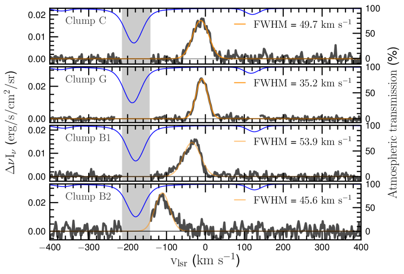
Figure 2: Medium-resolution H₂ S(5) 6.90952 $\mu$m ($\nu=1447.28$ cm^-1) spectra of (from top to bottom) clumps C, G, B1, and B2 in IC 443. In each panel, the background-subtracted intensity is shown in black. The intensity is in units of line brightness per spectral resolution element, $\Delta\nu I_{\nu}$, where $\Delta\nu=0.11$ cm^-1. The S(5) lines are marginally resolved at the resolution shown here. The atmospheric transmission is shown as a blue curve scaled to 100% at the top of each panel. The grey region shows where the transmission is less than 50%, which is where the background subtraction is less accurate. The orange line shows a Gaussian fit with full width at half-maximum intensity (FWHM) labeled.

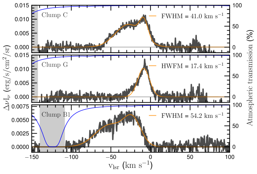
Figure 3: High-resolution H₂ S(5) 6.90952 $\mu$m ($\nu=1447.28$ cm^-1 spectra of (from top to bottom) clumps C, G, and B1 in IC 443. In each panel, the background-subtracted intensity is shown in black. The intensity is in units of line flux per resolution element, $\Delta\nu I_{\nu}$, where $\Delta\nu=0.022$ cm^-1. The S(5) lines are very well resolved at this resolution. The atmospheric transmission is shown as a blue curve scaled to 100% at the top of each panel. The grey region shows where the transmission is less than 50%, which is where the background subtraction is less accurate. The spectra are shown versus the velocity with respect to the local standard of rest (LSR) relative to nearby stars. The atmospheric absorption features appear at different velocities in each panel because they were observed on different dates, when the velocity of Earth relative to the LSR differed. The orange line shows a 2-Gaussian fit, with the FWHM of the wider component labeled.

Figure 3 shows the high-resolution spectra for the 3 IC 443 clumps that were detected at high resolution. These spectra cover the same positions as those in Figure 2. All positions were observed until a high signal-to-noise was obtained. For the position with the faintest emission in medium-resolution, IC 443 B2, the high-resolution spectrum did not show a convincing detection. The line would have been detected at high resolution if it were narrower than 12 km s^-1, so we conclude that the line from IC 443 B2 is both broad and significantly shifted from the pre-shock velocity, as determined from the medium-resolution observations.

Finally, we estimate the amount of extinction by dust and its effect on the observed line brightness. One reason that shocks into dense gas have remained an observational challenge is that they occur, by construction, in regions of high column density. Among the known supernova-molecular cloud interactions, IC 443 has relatively lower extinction, making it accessible to near-infrared (and, toward the NE, even optical) study. The extinction toward the shocks must be known in order to convert the measured brightness into emitted surface brightness, and to make an accurate comparison of ratios of lines observed at different wavelengths. For the prominent shocked clumps in IC 443, the estimated visible-light extinctions are $A_{\rm V}$=13.5 for Clump C and B and $A_{\rm V}$=10.8 for clump G (Richter et al., 1995a). At the wavelength of the H₂ S(5) line we observed with SOFIA, the extinction is only 0.2 magnitudes, so the observed brightness is only 20% lower than the emitted.

4 Predictions of MHD shock models for IC 443

To understand the implications of our observations in terms of physical conditions in the shock fronts, we proceed as follows. First, we assess the likely range of physical properties of the pre-shock gas and the shocks that are driven into it. Then, we generate shock models a priori given those physical conditions. Then in §6, we compare the shock models to the observations and discuss their implications.

4.1 Conditions of the shocked and pre-shock material

The properties of the gas before being impacted by the SN blast wave are of course not known; however, there is some direct evidence. Lee et al. (2012) measured the properties of nearby, small molecular clouds that are largely unshocked. The cloud they named SC05, for example, lies between shock clumps B and C; it was identified from CO(1–0) observations as a 13 $M_{\odot}$, cold clump with average density $\langle n_{{\rm H}_{2}}\rangle\sim 10^{3}$ cm^-3. There also must exist higher-density cores within SC05 in order to explain emission from HCO⁺, which has a critical density for excitation of $7\times 10^{5}$ cm^-3. In the interpretation by Lee et al. (2012), SC05 is what shock clumps B and C looked like, before they were crushed by the SN blast wave. Cloud SC05 is at an LSR velocity of -6.2 km s^-1 , which we will take as the nominal pre-shock velocity of the ambient gas. The CO(1–0) velocities for the ambient clouds around IC 443 have a range of about $\pm 3$ km s^-1 with respect to the average.

As mentioned in the Introduction, the pressure of the IC 443 blast wave appears inadequate to drive a blast wave that can accelerate gas with the densities of a molecular cloud. There are two keys to understanding the broad molecular lines.

(1) Enhancement of pressure at the clump shock: Moorhouse et al. (1991) and Chevalier (1999) showed that the part of the supernova remnant shell that impacts the clump is caught between the impetus of the expanding shell and the inertia of the clump, and the pressure in the slab of gas being driven into the clump is enhanced, relative to $p_{\rm ram}$, by a factor

$$\frac{p_{c}}{p_{\rm ram}}=\frac{n_{c}}{n_{0}}\left[1+\left(\frac{n_{c}}{n_{\rm shell}}\right)^{\frac{1}{2}}\right]^{-2},$$ (4)

where $n_{\rm shell}$ is the density of the shocked gas of the shell being driven into the clump. We use the electron density of the shocked gas, based on optical spectroscopy of [S II] in the shocked filaments (Fesen & Kirshner, 1980), to set $n_{\rm shell}=100$ cm^-3 . Given the uncertainty in the preshock density for the overall supernova shell, we use a value $n_{0}=2$ cm^-3  that is within the range 0.25 to 15 cm^-3  of X-ray, optical, and radio constraints; this value corresponds to a supernova remnant age of 10,000 yr. The pressure enhancement is crucial, because otherwise, as explained above, the ram pressure of the blast wave is insufficient accelerate dense molecular gas to the observed velocities.

(2) A range of densities for the clumps: It is naturally expected that a molecular clump is not an instantaneous rise in density from that of the interclump medium to a single clump density. Rather, the dense clumps are more likely to be complicated structures with fractal or filamentary shape and density gradients. In this case, a wide range of shock velocities is expected. Tauber et al. (1994) considered the case of a centrally condensed clump with radial profile, and showed qualitatively that a bow-shock structure is expected, with the lower-density gas swept from the dense core away from the explosion center. In addition to the structural implication of a range of densities, a much wider range of physical conditions is expected from a shocked clump than would arise from an isolated shock into a uniform clump of high density. The configuration would lead to emission along the same line of sight from gas with physical properties that cannot coexist in the same location but rather arise from separate shocks into portions of the clump that have different densities.

Using equations 2 to 4, the shock ram pressure and the pressure enhancement for shocks into molecular clumps with a range of densities are listed in Table 3. We are not considering the topology of the cloud, where layers at different densities that are shocked first would alter the properties of the shocks into ‘downstream’ portions of the cloud; instead, for this initial calculation, we imagine each part of the cloud experiencing the direct blast wave simultaneously. Table 3 lists the shock speed, $v_{s}$, into the gas at each density, ranging from 10 km s^-1 in the highest-density gas up to 100 km s^-1 in the lower-density, but still molecular, gas. The highest density into which a shock front will be driven is the one for which the pressure drives a Mach-1 sound wave into the clump, i.e. $v_{s}$ is greater than the sound speed. Using equations 3 and 2 for the shock pressure and speed, this condition becomes

$$n_{c}<5\times 10^{6}\left(\frac{T_{c}}{10\,{\rm K}}\right)^{-1}\left(\frac{p}{p_{\rm ram}}\right)\,{\rm cm}^{-3}.$$ (5)

At densities greater than $10^{3}$ cm^-3, the preshock material was no warmer than diffuse molecular clouds, which have $T_{c}\sim 100$ K, and likely they were as cold as molecular clouds, which have $T_{c}\sim 20$ K; therefore, shocks are driven into gas up to densities $n_{c}\sim 10^{6}$ cm^-3, which we take as the upper density for our models.

To give an idea of the size of the shocked region and the relative locations of shock fronts into different densities, Table 3 then lists the distance that the shock front would travel, in $10^{3}$ yr, into gas of each density. The actual age of the shocks is not known, but should be less than the age of the SNR and more than the time since the shocks were first observed—that is, in the range 45 to 40,000 yr—so $10^{3}$ yr is a useful illustration that will show the effects of early-time shock evolution. We further list the separation of the various shock fronts on the sky, relative to the shock into 6,000 cm^-3 gas. Relative to the shock into 6,000 cm^-3 gas, the shocks into higher-density gas (i.e., the molecular shocks) will be in the ‘upstream’ direction (negative separation), while shocks into lower gas (i.e., the ionic shocks) will have moved ‘downstream,’ further away from the original SN explosion site. Table 3 shows that only observations at the several-arcsec angular resolution and several km s^-1 spectral resolution will distinguish the shocks with densities in the $10^{3}$–$10^{5}$ cm^-3 range. This is precisely where the SOFIA/EXES observations are unique.

Table 3: Shock speeds into different densities for IC 443

$n_{c}$	$p/p_{\rm ram}$	$v_{s}$	$d$($10^{3}$ yr)	separation
(cm-3)		(km s-1)	(pc)	(′′)
500	24	100	0.10	8
2,000	33	60	0.061	3
6,000	38	40	0.042	0
20,000	43	22	0.022	-2
100,000	46	10	0.010	-4

5 MHD shock model predictions

We computed MHD shock models using the Paris-Durham shock code, which incorporates a wide range of heating and cooling mechanisms and a full network of astrochemistry (Flower & Pineau des Forêts, 2003, 2015; Lesaffre et al., 2013; Godard et al., 2019). Apart from using the specific conditions (pre-shock density and shock velocity) for IC 443, we used the following adaptations relative to the ‘nominal’ parameters in the model. First, we use an elevated cosmic-ray ionization rate, $\zeta=2\times 10^{-15}$ s^-1, based on the observations of H${}_{3}^{+}$ (Indriolo et al., 2010). The effect of photoionization on the shocked gas is included, because it was shown that irradiated shocks have different chemistry (Lesaffre et al., 2013). The pre-shock magnetic field was set according to $B\simeq 1n_{\rm H}^{0.5}$ $\mu$G, where $n_{\rm H}$ is the pre-shock density, $n_{\rm H}=n_{\rm H{\small I}}+2n_{{\rm H}_{2}}$. an approximate match to observations of molecular clouds with densities in the $10^{3}$ to $10^{5}$ cm^-3 range (Crutcher, 2012). Because the SN explosion was relatively recent, the time required to establish a steady-state shock front is, for some combinations of density and shock speed, longer than the age of the supernova remnant. We therefore consider non-steady shock models that evolve only up to a time $t$, and we ran models for $t=10^{3}$ and $10^{4}$ yr. The age of the SN explosion has been estimated in the range $4\times 10^{3}$ to $3\times 10^{4}$ yr (Troja et al., 2008; Chevalier, 1999), and it took some time for the shock front to propagate to the distance from center where we observe the shock clumps now. The $10^{3}$ yr models would apply if the blast wave reached the clumps at 75% of the lower-estimated age of the SN explosion and 96% (i.e. very recently) of the upper-estimated age of the SN explosion. The $10^{4}$ yr models are older than the lower-estimated age of the SN explosion (so they cannot apply if that age is correct) and 67% of the upper-estimated age of the SN explosion. the SN explosion.

Table 4: Properties of model shocks for different densities

$n_{c}$	$v_{s}$	$\langle z\rangle$	$I({\rm S}5)$	FWHM	$t_{\rm steady}$	Shock Type
(cm-3)	(km s-1)	(pc)	($10^{-3}$erg s cm-2s r-1)	(km s-1)	(yr)
500	100	$\sim 0.1$	0.02	$\sim 1$	200,000	J
2,000	60	0.016	1.5	28	50,000	CJ
6,000	37	0.011	8.9	19	20,000	CJ
20,000	22	0.0018	9.8	10	5,000	CJ
100,000	10	0.0003	7.7	4	1,000	C

The shocks into the gas have different character depending on their physical conditions. A key condition is whether the shock can be treated as a single fluid (in which case all material moves at the speed of the primary mass contributor, which is H₂) or the ions and neutrals separate (in which case a 2-fluid, C-type shock develops). The distinction occurs for shocks with speed lower than the magnetosonic speed,

$$v_{m}^{2}\equiv c_{s}^{2}+v_{Ac}^{2}$$ (6)

where $v_{Ac}$ is the effective Alfvén speed (Lesaffre et al., 2013). The dynamics of the shock depend critically on the mass density of ionized particles that couples with the magnetic field. The gas in molecular clouds is ionized by cosmic rays to an ionization fraction $x=n_{i}/n_{\rm H}\lower 2.15277pt\hbox{$\;\buildrel<\over{\sim}\;$}10^{-7}$. With the gas predominantly neutral, charged dust grains become the dominant mass loading onto the magnetic fields (Guillet et al., 2007). The mass-weighted average absolute value of the grain charge, $\langle|Z|\rangle$, is of order unity under conditions of low radiation field (cf. Draine & Sutin, 1987; Ibáñez-Mejía et al., 2019). We write the magnetic field in terms of the gas density as, $B=b(n_{\rm H}/{\rm cm}^{-3})^{1/2}$ $\mu$G, a scaling that applies to flux-frozen magnetic fields, with observations showing average magnetic fields consistent with $b$ of order unity (Crutcher, 2012). The criterion for a C-type shock, $v_{s}<v_{m}$, then can be expressed as a limit on the magnetic field strength:

$$b>\frac{v_{s}}{19\,{\rm km~{}s}^{-1}}\left[100x+\langle|Z|\rangle\frac{100}{[{\rm G}/{\rm D}]}\right]^{\frac{1}{2}}\left(1-\frac{1}{M^{2}}\right)^{\frac{1}{2}},$$ (7)

where $[{\rm G}/{\rm D}]$ is the gas-to-dust mass ratio, and $M=v_{s}/c_{s}$ is the Mach number (which is greater than 1 as enforced by equation 5). The first term in the square brackets is for ionized gas; in molecular clouds, $x<10^{-6}$ so this term is small. The second term in the square brackets is for charged grains and is of order unity; this term will dominate unless the gas is highly ionized or the grains are uncharged, neither of which are likely to apply.

Referring to the preshock conditions from Table 3, we see that two-fluid shocks occur (i.e. the inequality in equation 7 applies) for magnetic field strength $B>100$ $\mu$G for $n_{c}=10^{3}$ cm^-3 and $B>350$ $\mu$G for $n_{c}=10^{5}$ cm^-3, comparable to the observed average fields in molecular clouds. If we consider the environment around the IC 443 progenitor as having been similar to the Orion Molecular Cloud, average magnetic field strengths of 300 $\mu$G were derived from dust polarization (Chuss et al., 2019). It is thus expected that the conditions for C-type shocks are present, which is important for generating a significant layer of dense, warm, molecular gas that generates wide H₂ lines. The magnetic field in the shocked molecular gas was directly detected via the Zeeman effect for radio-frequency OH masers, yielding strengths of 200 to 2200 $\mu$G (Brogan et al., 2000, 2013). For the shocks model calculations in this paper, we set the magnetic field input parameter $b=3$, which allows for C-type shocks to develop.

The results of the shock models for the input parameters from Table 3 relevant to IC 443 are as follows. First, the shocks are single-fluid J-type for densities lower than $10^{3}$ cm^-3, because the shock speeds are greater than the magnetosonic speed, unless the magnetic field is significantly enhanced relative to a nominal molecular cloud. Second, the shocks for moderate-density ($10^{3}$ to $10^{4}$ cm^-3) gas are non-steady, because they do not have time to develop to steady state within $10^{3}$ yr. Third, shocks into high-density ($\gtrsim 10^{5}$ cm^-3) gas are steady-state because cooling is so fast that they develop within $10^{3}$ yr. Table 4 lists basic model properties including the spatial extent of the shock front, the total brightness of the S5 line of H₂, and the time it takes for a steady-state shock to develop (Lesaffre et al., 2004). The shock fronts are generally thin; at the distance of IC 443, the shocks into $10^{3}$ cm^-3 clumps would subtend, if viewed edge-on, $2.2^{\prime\prime}$, which would be nearly resolved in the Spitzer/IRAC observations and resolved to SOFIA/EXES and high-angular-resolution near-infrared images (Richter et al., 1995a), while the shocks into denser gas would be unresolved.

In order to calculate and understand the predicted line profile, we use the local emissivity $\mathcal{E}(z)$ versus distance behind the shock, $z$. Figure 4 shows the emissivity versus distance for shocks with properties listed in Table 3. Key characteristics of the shock models include the following. (1) There is an offset of the emitting region behind the shock front, due to the delayed reaction of the ions and neutrals; this offset increases with decreasing preshock density (for fixed shock ram pressure). (2) The width of the emitting region increases with decreasing preshock density. (3) For densities $10^{3}$ to $10^{4}$ cm^-3, the distinct characteristics of a CJ-type shock appear as a spike in emissivity (due to high temperatures) far behind the shock front. This spike is the J-type component of the CJ shock and appears because we only allowed the shock to evolve for $10^{3}$ yr, based upon arguments above that this is the likely age of shocks given the age of the supernova explosion. To clearly show the effect of shock age, Figure 5 shows the emissivity versus distance for the preshock density $10^{4}$ cm^-3 case at three different ages. For the IC 443 blast wave, the CJ characteristics are expected to be mild for shocks into $10^{4}$ cm^-3 and more prominent for $10^{3}$ cm^-3 gas. (4) Finally, for the lowest density we considered, $10^{2}$ cm^-3, the temperature behind the shock is so high that molecules are dissociated and atoms ionized, leading to a J-type shock with an extended recombination zone. The H₂ emission only arises far behind the shock in the region after the gas has recombined and cooled to $\sim 300$ K and compressed to where molecules can reform, at $z\sim 0.1$ pc (Hollenbach & McKee, 1989), and the total emission from that shock is two orders of magnitude fainter (Table 4) than for the C (and CJ) shocks. Note that the reformation of H₂, behind J-type shocks into gas with densities less than $10^{3}$ cm^-3, takes $10^{6}$ yr, so a steady-state J shock of this sort cannot exist for a supernova remnant like IC 443. Indeed, molecule reformation would only be complete for gas with density $>10^{5}$ cm^-3, and shocks into gas with such high density are affected by the associated strong magnetic field so that they do not destroy H₂.

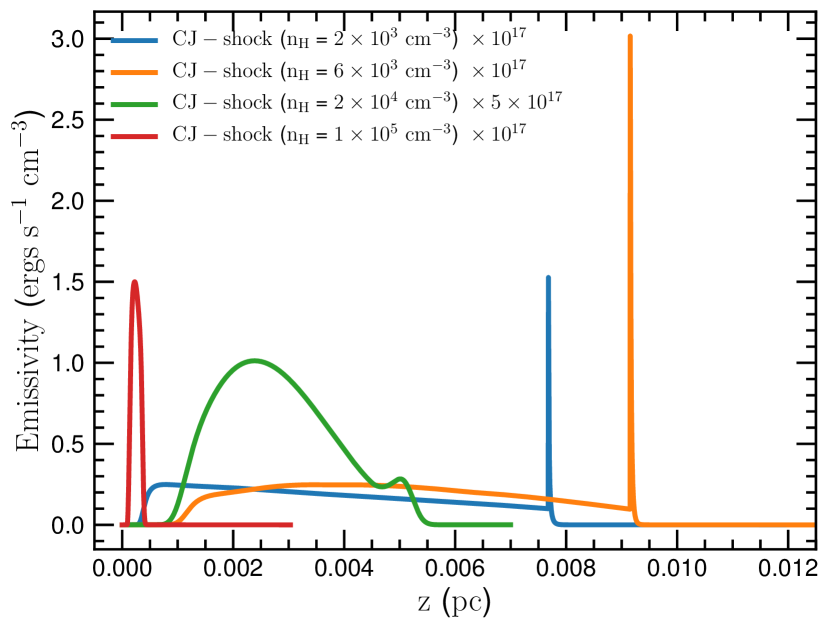
Figure 4: Emissivity of the H₂ S(5) line behind shocks with properties listed in Table 3. The shock into the highest-density, $10^{5}$ cm^-3, gas is in a compressed region due to rapid cooling of the gas. Shocks into gas with density greater than $10^{5}$ down to $10^{3}$ cm^-3 are predominantly C-type, and the H₂ emission arises from a broad region whose size increases for decreasing density. The shocks into gas with density $\leq 10^{4}$ cm^-3 show an additional, spatially-narrow spike at the greatest distance ($z$) behind the shock front; this is the J-type shock that is present because the shock age ($10^{3}$ yr) is shorter than the time required to fully develop a steady-state C-type shock.

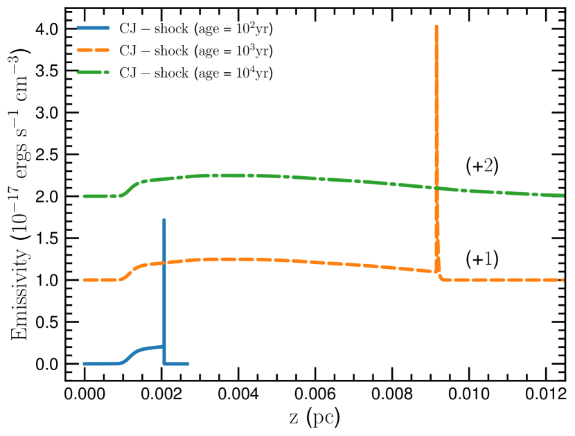
Figure 5: Emissivity of the H₂ S(5) line behind shocks into gas with preshock density $6,000$ cm^-3 and shock velocity 37 km s^-1 with ages $10^{2}$, $10^{3}$, and $10^{4}$ yr. The upper curve shows the oldest model, which approaches the shape of a fully-developed, steady-state C-type shock. The lowest curve shows the youngest model, which has the distinct CJ-type shape: the broad C-type region is truncated, and the J-type portion is relatively prominent. For the expected age of IC 443 shocks, shown in the middle curve, the shock is almost fully developed into C-type but with a small J-type component.

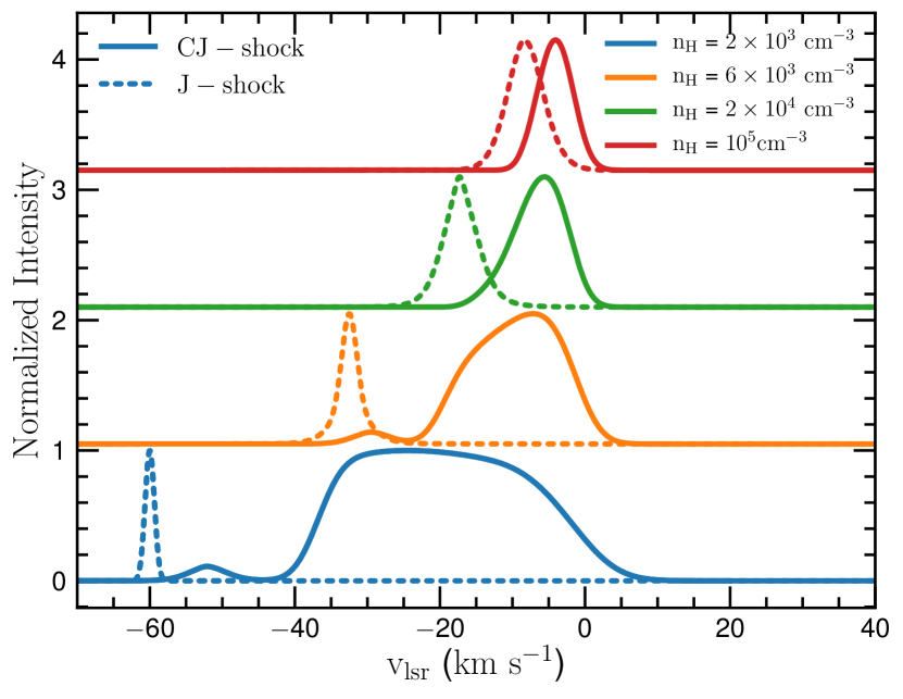
Figure 6: Velocity profiles of the H₂ S(5) lines produced by shocks with properties listed in Table 3. The models are for face-on shocks, moving toward the observer, and the horizontal axis is the projected (‘observed’) velocity in km s^-1  relative to the pre-shock gas at velocity zero. The velocities with significant emission depend on the speed and temperature of the gas at each distance behind the shock (Fig. 4). The velocity profile for the highest-density shock is the most narrow and close to the zero velocity, due to rapid cooling of the dense gas. With decreasing density the shock becomes wider (because the same pressure drives faster shocks that heat the gas to higher temperature) and shifted to higher velocity. For the CJ-shock into $n_{c}=2,000$ and $6,000$ cm^-3 gas, small peaks near the shock velocity are the emission from the non-steady portion of the shock as was illustrated in Figure 4.

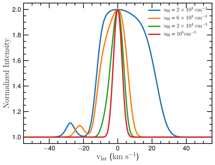
Figure 7: The same models as shown in Figure 6, shifted in velocity so that their peak is at 0 km s^-1. The most narrow line profile is for the shock into the densest gas, with a steady progression of increasing H₂ line width as pre-shock density decreases. The detailed shape of the line profiles relates to the post-shock temperature and density structure. For the shocks into $n_{c}=2,000$ and $6,000$ cm^-3 gas, small peaks in the predicted line profiles due appears near the shock velocity due to hot gas just behind the shock front; this gas is still noticeably far from its steady state. If allowed to evolve for several thousand years, the line profiles would be as wide on the negative-velocity side as it is on the positive-velocity side. The shifted profiles shown in this Figure are only for illustration of the line shape differences; for fitting observations, only the unshifted profiles in Figure 6 should be used.

With the emissivities, we can now calculate the velocity profiles of the H₂ S(5) lines by integrating over the line of sight:

$$I(v)=\int{\rm d}z\frac{\mathcal{E}(z)}{\sqrt{2\pi}\sigma(s)}e^{-\left[v-\left(v_{n}(z)-v_{s}\right){\rm cos}i\right]^{2}/2\sigma(z)^{2}}$$ (8)

where $i$ is the inclination of the shock front with respect to the line of sight, and $\sigma(z)$ is the thermal dispersion for gas at the temperature of neutral gas at distance $z$ behind the shock front. The spectrum of the H₂ emission lines contains key diagnostic details for the properties of the shock fronts. Figure 6 shows the H₂ S(5) line profiles from model shocks, and Table 4 lists the widths of the model-predicted lines. The predictions are for face-on shocks. For a shock front inclined relative to the line of sight, the line profile changes in a somewhat complicated manner that depends upon the emissivity and velocity at each distance behind the shock. However, to first order, the width of the line profile is not strongly affected by inclination of the shock relative to the line of sight, because the emission from each parcel of post-shock gas is isotropic, with velocity dispersion depending on its temperature.

For the lowest density in Table 3, $10^{2}$ cm^-3, the emission from the J-type shock can be roughly approximated by a Gaussian with very narrow ($\sim 1$ km s^-1) velocity dispersion corresponding to the $\sim 300$ K temperature of the molecule reformation region (Hollenbach & McKee, 1989). The J-shock front is at velocity $v_{0}+v_{s}$, where $v_{0}$ is the velocity of the ambient, pre-shock gas. The molecule reformation region where the gas has slowed would have velocity $v_{0}+v_{s}/4$ (for a 4:1 density increase and conserving momentum), so it would appear at approximately -30 km s^-1. The amount of H₂ reformed behind such a shock is expected to be very small, because the age of the supernova remnant is only 1% of the time for the molecules to form.

6 Comparison of Shock Models to Observations

First, we compare the predicted brightness of the H₂ S(5) line to that observed for the shock clumps in IC 443. The well-calibrated Spitzer spectrum of IC 443C has $I({\rm S}5)\simeq 2\times 10^{-3}$ erg s^-1 cm^-2 sr^-1 (Neufeld et al., 2007), and our SOFIA/EXES spectrum (at higher angular and spectral resolution) has $I({\rm S}5)\simeq 4\times 10^{-2}$ erg s^-1 cm^-2 sr^-1. The models with $n_{c}>10^{3}$ cm^-3 can explain the observed brightness, with modest secant boosts to account for inclination of the shock front with respect to the line of sight. For comparison to older shock models, the prediction from Draine et al. (1983) for shocks into gas with $n=10^{4}$ cm^-3 and $v_{s}=37$ km s^-1 agree well with the Paris-Durham shock code. The J-shock models from Hollenbach & McKee (1989) are significantly different: for $n=10^{3}$ cm^-3 and $v_{s}=60$ km s^-1, they predict a brightness $10^{3}$ times lower than the observed lines; the assumptions in those J-type models and the time required to reach a steady state lead to predicted brightness far too low to explain the observed lines.

Second, we compare the velocity width of the lines to the model predictions. The observed widths are in the range 17 to 60 km s^-1 FWHM (with non-Gaussian lineshapes extending to higher velocities. The model predictions for shocks into gas with density in the range $10^{3}$ to $10^{5}$ cm^-3  (Table 4) can explain most of this range. The narrow lines from reformed molecules in a 300 K layer behind J-type shocks (Hollenbach & McKee, 1989) cannot produce these lines because they are too narrow. Similarly, shocks into higher-density gas may be present but cannot contribute much of the observed lines. This conclusion is in accord with that derived in the previous paragraph based upon the line brightness.

Now, we can use the new a priori theoretical predictions for the detailed shape of shock line profiles to directly compare to the observed spectra. We assume the pre-shock gas is within $\pm 3$ km s^-1  of -6.2 km s^-1 based upon the small, unshocked clouds near IC 443 (Lee et al., 2012). The models are computed for ‘face-on’ shocks that are infinite and plane-parallel. The observed brightness can be enhanced relative to the face-on value by the secant of the tilt, $i$, between the line of sight and the shock normal: $I_{\rm obs}=I_{0}{\rm sec}(i)$. In practice, the pre-shock gas is likely to be structured with a range of densities and finite physical scales, and the shocks have non-trivial thickness. Thus the effect of the inclination and the beam filling factor partially cancel each other out. If the shock thickness is $z$ (see Figure 4), and the pre-shock clump size in the plane of the sky is $L$, IC 443 is at distance $D$, and the beam size is $\theta_{b}$, then, for an edge on shock, the beam filling factor is $z/D\theta_{b}$ and the boost in brightness due to inclination is $L/z$. The product of beam filling factor and secant boost is $L/D\theta_{b}$, which is the maximum boost in brightness relative to a face-on shock. The 2MASS, Spitzer, and Herschel images show structure at the $L/D\lower 2.15277pt\hbox{$\;\buildrel<\over{\sim}\;$}2^{\prime\prime}$ scale, and the slit size for SOFIA spectra is $2.4^{\prime\prime}$, so $L/D\theta_{b}\lower 2.15277pt\hbox{$\;\buildrel<\over{\sim}\;$}0.8$ is of order unity. The net effect of the inclination effects on the shock brightness, relative to a face-on shock, is that it can be lower by a factor of $\sim 0.8$ or bright by a factor of ${\rm sec}(i)$ up to a factor of $L/D\theta_{b}\lower 2.15277pt\hbox{$\;\buildrel<\over{\sim}\;$}10$. Thus there is very limited flexibility in using a shock model to explain the observed brightness: a successful shock model must be between 80% and 1000% of the observed brightness, in absolute units.

Table 5: Fits of shock models to H₂ S(5) from IC 443 clumps

Clump	$n_{H}$	$v_{s}$	shock age	Viewing angle	Scaling Factor	shock type
	(cm-3)	(km s-1)	(yr)	(o)
C	2,000	60	5,000	0	1.07	CJ
	10,000	31	3,000	0	0.3	CJ
G	6,000	37	3,000	65	0.3	CJ
	2,000	60	5,000	60	0.33	CJ
B1	2,000	60	5,000	0	0.14	CJ
	2,000	60	//	//	//	J
B2	400	110	//	//	//	J

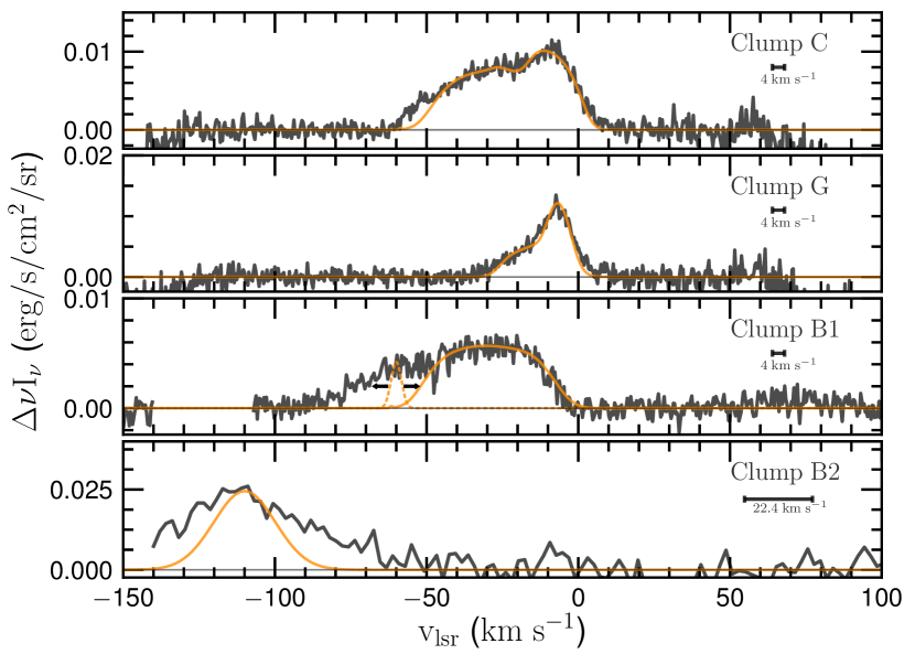
Figure 8: Shock model fits to H₂ S(5) emission from clumps C, G, B1, and B2 (top to bottom) in IC 443. The model components are listed in Table 5. The spectral resolution is indicated by a scale bar to the right; for clump B2, only the ‘medium’ resolution was observed. For clumps C, G, and B1, broad emission at velocities -50 to 0 km s^-1 is due to CJ shocks with dynamics strongly affected by the magnetic field. The orange line shows the model fits described in the text. For clump B2, there is no significant emission in that velocity range, and model is a J-type shock (with no magnetic field). For clump B1, we show a fit including CJ shocks for the -50 to 0 km s^-1 range together with a single J-type shock for illustration; the emission from -90 to -50 km s^-1 can be explained by a sum of such J-type shocks into a range of densities (indicated by the arrows next to the J0shock model, pointing toward lower and higher velocity).

We can improve the agreement between the models and the observations by allowing freedom in inclination of the shock front with respect to the line of sight, by combining shock models representing shocks into different-density gas, and by adjusting the pre-shock gas properties. We restrict parameter tuning so that only models that have properties that are within reasonable expectation for IC 443 are considered. We only permit a $\pm 3$ km s^-1 shift in the ambient gas velocity, which proves to be a powerful constraint now that we have a full theoretical model for the velocity profile of the shocked gas. We require the shock age to be less than the age of the supernova remnant, estimated as 10,000 yr. Compared to the a priori models in §4, which fixed the age at 1,000 yr, allowing for older shocks allows the non-steady solutions for shocks into $10^{3}$ and $10^{4}$ cm^-3 gas to evolve toward full, steady-state solutions. This more-complete evolution increases the width of the emergent H₂ line (and removes the J-type contribution at the ambient velocity).

The model fits to the observed H₂ lines are shown in Figure 8, with parameters summarized in Table 5. The ‘scaling factor’ in this table can be attributed to the boosts and decrements due to inclination of the shock and finite extent of the clump as discussed earlier. The emission observed at velocities -50 to 0 km s^-1 can be explained as CJ-type shocks into gas with pre-shock densities in the range $10^{3}$ to $2\times 10^{4}$ cm^-3. range of those observed for the pre-shock gas; the pressure of the shock fronts is specified from the a priori estimates based on X-ray and optical properties of the supernova remnant. For each model, a shock age was derived by fit. The shocks into the highest-density gas could actually be younger, because they rapidly reach their steady state. But the shocks into the $10^{3}$ cm^-3 gas show ages of 5,000 yr. This age is older than some estimates of the entire age of the supernova remnant. Allowing some time for the blast wave to reach the preshock cloud, our results support the older estimates that the supernova explosion occurred more than 6,000 yr ago.

The CJ-type shocks are all for magnetic fields oriented perpendicular to the shock: $\vec{B}\bot\vec{v_{s}}$. For clump B2 and for the most-negative velocity emission from clumps B1 and C, emission from J-type shocks is required. The critical difference, in terms of observable properties, is that when the dynamics of the shocked gas are dominated by the magnetic field, the gas is gently and steadily accelerated, leading to a broad line profile that spans from the velocity of the preshock gas up to a significant fraction of the shock velocity. On the other hand, if the magnetic field is oriented so that it does not affect the shock dynamics, i.e. $\vec{B}\parallel\vec{v_{s}}$, then the gas is accelerated to the shock speed. The observed line profile is then a relatively narrow component centered at a velocity shifted from the preshock gas by $v_{s}{\rm cos}(i)$. Figure 5 shows how such shocks could contribute to the H₂ line profiles. It is particularly notable that clump B2 displays only what we interpret as J-type shock, while clump B1 is primarily CJ-type. We infer that the direction of the magnetic field relative to blast wave changes significantly between B2 and B1.

7 Discussion and Conclusions

7.1 Properties of shocks in IC 443

There is a long history of spectroscopic observations of IC 443 and attempts to determine the nature of the shock fronts into them. We focused in this paper on addressing the question, initially posed in our observing proposal: What type of shock produces the molecular emission from supernova remnants interacting with molecular clouds? We generated a priori predictions of the velocity profiles of the H₂ S(5) line, and compared them to new, SOFIA/EXES observations at high spatial ($2.4^{\prime\prime}$) and spectral ($R=7\times 10^{4}$) resolution. We found that the CJ type shock into $10^{3}$ density and C-type into $10^{4}$ density are the best fit to most of the emission, with the high-velocity wings requiring J-type shocks into gas with density $10^{3}$ cm^-3 and lower. In these shocks, the S(5) line of $H_{2}$ is predicted to be one of the brightest spectral lines and is therefore energetically significant as an important coolant in the shocked gas.

In comparison to previous work on the molecular shocks in IC 443:

• Richter et al. (1995b) detected the H₂ S(2) line and compared with higher-excitation lines to infer a partially-dissociating J-type shock into gas with density $4\times 10^{3}$ cm^-3; our results support the inference of a J-type shock based on the detailed line profile and modern theoretical modeling.

• Cesarsky et al. (1999) used Infrared Space Observatory to measure intensities of pure rotational lines S(2) through S(8) for IC 443. Generally consistent with our results, they derived densities of order $10^{4}$ cm^-3 with shock speeds 30 km s^-1 and ages 1000-2000 yr; indeed, their paper contained one of the first applications of a non-steady CJ-shock.

• Snell et al. (2005) observed H₂O at high velocity resolution using SWAS, showing emission, from a $4^{\prime}$ region centered on clump B, with velocities up to 70 km s^-1; they interpret the emission with a range of shock types and infer properties of the oxygen state in the preshock gas. Our results can help explain the SWAS observations and the HCO$+$ and other broad molecular lines. The SWAS beam includes our position B1 and extends almost to B2, so the H₂ emission covers the entire range of velocities where H₂O and HCO⁺ were seen, and more. As for H₂, most of the broad-line emission arises from CJ-shocks into dense gas, while the most extreme velocities are from J-shocks into moderate-density gas.

• Rosado et al. (2007) made moderate ($R=10^{4}$) resolution observations of the vibrationally excited H₂1–0 S(1) line toward IC 443C. The brightest emission in their image, was only marginally resolved but consistent with our much higher-resolution observation of the S(5) line.

7.2 Relationship between molecular cloud shocks and cosmic rays

A remarkable achievement in high-energy astronomy was the first spatially-resolved image of a supernova remnant, showing that TeV particles originate from the portion of IC 443 coinciding with shocked molecular gas (Albert et al., 2007; Acciari et al., 2009). A joint analysis of the VERITAS and Fermi data documented the challenges in combining the high energy data and yielded a map of the relativistic particle distribution (Humensky & VERITAS Collaboration, 2015). In particular, the region around clump G stands out as a prominent TeV peak. The TeV photons could be produced by interaction of cosmic rays produced in the SN explosion with a dense cloud, in which case the TeV photons are pion decay products (Torres et al., 2008). By localizing the source of the high-energy $\gamma$ rays to the molecular interaction region (what we call the $\omega$ shaped ridge), as opposed to the northeastern rim where the radio emission is far brighter, an electron bremsstrahlung origin (in which the high-energy emission should arise from the same place as the radio synchrotron emission) is ruled out, in favor of a pion decay origin, meaning that localized high energy $gamma$ rays and TeV photons trace the origin of (hadronic) cosmic rays (Tavani et al., 2010; Abdo et al., 2010). The prominence of clump G in TeV photons can be explained by that shock front both having dense gas and being nearly edge-on, so that the path length is highest; it is also the brightest of the shocked clumps in the H₂ S(5) line, which is the brightest emission line from such shocks.

The general observational correspondence between the shocked molecular gas distribution and cosmic rays is only at the scale of several arcminutes. Our results on the H₂ emission from IC 443 show that the site of the shocks into dense gas, which may be related to cosmic ray acceleration, are the portions of the molecular cloud with preshock densities of order $10^{3}$ to $10^{5}$ cm^-3 with shock speeds of 20 to 60 km s^-1 . The H₂ emitting region tracing the shocks into dense gas is structured at the $2^{\prime\prime}$ scale (resolution limited) in regions with size of order $30^{\prime\prime}$ (the size of the bright region in Clump C or G in the Spitzer image). The angular resolution of the current state-of-the-art Cerenkov telescopes, including HESS, MAGIC, and VERITAS, is approximately $5^{\prime}$ for localizing 1 TeV particles entering the atmosphere. The new state of the art will become the Cerenkov Telescope Array (CTA Consortium & Ong, 2019), which will have an angular resolution approximately $3^{\prime}$ at 1 TeV and $2^{\prime}$ at 10 TeV. There is a fundamental limit to the Cerenkov technique for localizing cosmic particles. Once all Cerenkov photons generated by particles upon entering the atmosphere are detected, there is no further improvement of the centroids. This limit was estimated to be approximately $20^{\prime\prime}$ at 1 TeV and $10^{\prime\prime}$ at 10 TeV (Hofmann, 2006). We expect that if the shocks into dense gas are intimately related with the comic ray origin, the structure in the TeV images will continue to be more detailed up until the ultimate limit of the Cerenkov telescopes is reached.

It is likely that cosmic rays and dense molecular shocks are two integrally related phenomena, linked by the strength of the magnetic field. Cosmic ray acceleration requires a strong magnetic field; without a strong field, the Lorentz force felt by high-energy particles will have a radius of curvature (Larmor radius) so large that the particles will hardly be deflected before leaving the region ($R>R_{L}$) for most astronomical objects. Magnetic field amplification is highest for fast shocks into dense gas (Marcowith et al., 2018). As for the broad molecular line emission, we showed above that strong (of order mG) magnetic fields are required, so that shocks driven by enough pressure to accelerate the gas do not dissociate the molecules in the process. A relativistic particle of energy $10^{15}$ eV in a region with magnetic field strength 1 mG will have a Larmor radius 0.001 pc, which is of the same order as the thickness predicted (in Fig. 4) for C-type shocks into gas with the properties of the molecular cloud around IC 443. Thus the common elements for cosmic ray acceleration and broad molecular lines are a strong magnetic field and dense gas, which conditions are both present when supernova-driven shock waves impinge upon molecular clouds.

7.3 Future prospects

The connection between cosmic ray origin and feedback of star formation into molecular clouds will make understanding of supernova shocks into dense gas of continuing interest. One curious observation that we can now answer is, why are broad molecular lines from shocks always approximately 30 km s^-1 wide. Shocks faster than $\gtrsim 40$ km s^-1  into gas with a low magnetic field will be J-type and will destroy H₂ (Draine et al., 1983); given the emitted power increases steeply with shock velocity, we would expect molecular lines of $\lower 2.15277pt\hbox{$\;\buildrel<\over{\sim}\;$}40$ km s^-1 width and shifted relative to ambient gas.

Only with very high velocity resolution are such effects discernible. The brightest, broad molecular lines are from CJ-type shocks into dense gas, with magnetic field perpendicular to shock velocity. Unless the magnetic field is always perpendicular to the shock velocity, there should also be emission at more extreme velocities, due to gas that is shocked and not protected by the magnetic field. In future theoretical work, it should be possible to unify J-shock models (Hartigan et al., 1987; Hollenbach & McKee, 1989), for which the immediate post-shock region is dominated by atomic physics (ionization/recombination), with C-shock models (Godard et al., 2019), for which the post-shock gas is dominated by MHD and chemistry. Other theoretical work to better understand the shock physics involves simultaneous modeling of the H₂ (and other molecule) excitation and line profile, as well as 2-D modeling of emission from shocked clumps of shape more realistic than the 1-D slabs considered here (Tram et al., 2018).

References

- Abdo et al. (2010) Abdo, A. A., Ackermann, M., Ajello, M., et al. 2010, ApJ, 712, 459
- Acciari et al. (2009) Acciari, V. A., Aliu, E., Arlen, T., et al. 2009, ApJ, 698, L133
- Albert et al. (2007) Albert, J., Aliu, E., Anderhub, H., et al. 2007, ApJ, 664, L87
- Braun & Strom (1986) Braun, R., & Strom, R. G. 1986, A&A, 164, 193
- Brogan et al. (2000) Brogan, C. L., Frail, D. A., Goss, W. M., & Troland , T. H. 2000, ApJ, 537, 875
- Brogan et al. (2013) Brogan, C. L., Goss, W. M., Hunter, T. R., et al. 2013, ApJ, 771, 91
- Burton et al. (1988) Burton, M. G., Geballe, T. R., Brand, P. W. J. L., & Webster, A. S. 1988, MNRAS, 231, 617
- Burton et al. (1990) Burton, M. G., Hollenbach, D. J., Haas, M. R., & Erickson, E. F. 1990, ApJ, 355, 197
- Cesarsky et al. (1999) Cesarsky, D., Cox, P., Pineau des Forêts, G., et al. 1999, A&A, 348, 945
- Chevalier (1999) Chevalier, R. A. 1999, ApJ, 511, 798
- Chuss et al. (2019) Chuss, D. T., Andersson, B. G., Bally, J., et al. 2019, ApJ, 872, 187
- Crutcher (2012) Crutcher, R. M. 2012, ARA&A, 50, 29
- CTA Consortium & Ong (2019) CTA Consortium, T., & Ong, r. b. R. A. 2019, arXiv e-prints, arXiv:1904.12196
- Denoyer (1979) Denoyer, L. K. 1979, ApJ, 232, L165
- Dickman et al. (1992) Dickman, R. L., Snell, R. L., Ziurys, L. M., & Huang, Y.-L. 1992, ApJ, 400, 203
- Draine et al. (1983) Draine, B. T., Roberge, W. G., & Dalgarno, A. 1983, ApJ, 264, 485
- Draine & Sutin (1987) Draine, B. T., & Sutin, B. 1987, ApJ, 320, 803
- Ennico et al. (2018) Ennico, K., Becklin, E. E., Le, J., et al. 2018, Journal of Astronomical Instrumentation, 7, 1840012
- Fazio et al. (2004) Fazio, G. G., Hora, J. L., Allen, L. E., et al. 2004, ApJS, 154, 10
- Fesen & Kirshner (1980) Fesen, R. A., & Kirshner, R. P. 1980, ApJ, 242, 1023
- Flower & Pineau des Forêts (2003) Flower, D. R., & Pineau des Forêts, G. 2003, MNRAS, 343, 390
- Flower & Pineau des Forêts (2015) —. 2015, A&A, 578, A63
- Gaensler et al. (2006) Gaensler, B. M., Chatterjee, S., Slane, P. O., et al. 2006, ApJ, 648, 1037
- Giovanelli & Haynes (1979) Giovanelli, R., & Haynes, M. P. 1979, ApJ, 230, 404
- Godard et al. (2019) Godard, B., Pineau des Forêts, G., Lesaffre, P., et al. 2019, A&A, 622, A100
- Guillet et al. (2007) Guillet, V., Pineau Des Forêts, G., & Jones, A. P. 2007, A&A, 476, 263
- Hartigan et al. (1987) Hartigan, P., Raymond, J., & Hartmann, L. 1987, ApJ, 316, 323
- Hofmann (2006) Hofmann, W. 2006, in Towards a Network of Atm. Cherenkov Detectors VII, ed. B. Degrange & G. Fontaine, 393
- Hollenbach & McKee (1989) Hollenbach, D., & McKee, C. F. 1989, ApJ, 342, 306
- Humensky & VERITAS Collaboration (2015) Humensky, B., & VERITAS Collaboration. 2015, in 34th International Cosmic Ray Conference (ICRC2015), Vol. 34, 875
- Ibáñez-Mejía et al. (2019) Ibáñez-Mejía, J. C., Walch, S., Ivlev, A. V., et al. 2019, MNRAS, 485, 1220
- Indriolo et al. (2010) Indriolo, N., Blake, G. A., Goto, M., et al. 2010, ApJ, 724, 1357
- Lacy et al. (2002) Lacy, J. H., Richter, M. J., Greathouse, T. K., Jaffe, D. T., & Zhu, Q. 2002, PASP, 114, 153
- Lee et al. (2012) Lee, J.-J., Koo, B.-C., Snell, R. L., et al. 2012, ApJ, 749, 34
- Lesaffre et al. (2004) Lesaffre, P., Chièze, J. P., Cabrit, S., & Pineau des Forêts, G. 2004, A&A, 427, 157
- Lesaffre et al. (2013) Lesaffre, P., Pineau des Forêts, G., Godard, B., et al. 2013, A&A, 550, A106
- Lord (1992) Lord, S. D. 1992, Lord, S. D., 1992, NASA Technical Memorandum, 103957, 1
- Marcowith et al. (2018) Marcowith, A., Dwarkadas, V. V., Renaud, M., Tatischeff, V., & Giacinti, G. 2018, MNRAS, 479, 4470
- Moorhouse et al. (1991) Moorhouse, A., Brand, P. W. J. L., Geballe, T. R., & Burton, M. G. 1991, MNRAS, 253, 662
- Neufeld et al. (2007) Neufeld, D. A., Hollenbach, D. J., Kaufman, M. J., et al. 2007, ApJ, 664, 890
- Olbert et al. (2001) Olbert, C. M., Clearfield, C. R., Williams, N. E., Keohane, J. W., & Frail, D. A. 2001, ApJ, 554, L205
- Park et al. (2014) Park, C., Jaffe, D. T., Yuk, I.-S., et al. 2014, in Proc. SPIE, Vol. 9147, Ground-based and Airborne Instrumentation for Astronomy V, 91471D
- Reach et al. (2006) Reach, W. T., Rho, J., Tappe, A., et al. 2006, AJ, 131, 1479
- Rho et al. (2001) Rho, J., Jarrett, T. H., Cutri, R. M., & Reach, W. T. 2001, ApJ, 547, 885
- Richter et al. (2018) Richter, M. J., DeWitt, C. N., McKelvey, M., et al. 2018, J. Astron. Instrument., 7, 1840013
- Richter et al. (1995a) Richter, M. J., Graham, J. R., & Wright, G. S. 1995a, ApJ, 454, 277
- Richter et al. (1995b) Richter, M. J., Graham, J. R., Wright, G. S., Kelly, D. M., & Lacy, J. H. 1995b, ApJ, 449, L83
- Rosado et al. (2007) Rosado, M., Arias, L., & Ambrocio-Cruz, P. 2007, AJ, 133, 89
- Shinn et al. (2011) Shinn, J.-H., Koo, B.-C., Seon, K.-I., & Lee, H.-G. 2011, ApJ, 732, 124
- Snell et al. (2005) Snell, R. L., Hollenbach, D., Howe, J. E., et al. 2005, ApJ, 620, 758
- Swartz et al. (2015) Swartz, D. A., Pavlov, G. G., Clarke, T., et al. 2015, ApJ, 808, 84
- Tauber et al. (1994) Tauber, J. A., Snell, R. L., Dickman, R. L., & Ziurys, L. M. 1994, ApJ, 421, 570
- Tavani et al. (2010) Tavani, M., Giuliani, A., Chen, A. W., et al. 2010, ApJ, 710, L151
- Torres et al. (2008) Torres, D. F., Rodriguez Marrero, A. Y., & de Cea Del Pozo, E. 2008, MNRAS, 387, L59
- Tram et al. (2018) Tram, L. N., Lesaffre, P., Cabrit, S., Gusdorf, A., & Nhung, P. T. 2018, MNRAS, 473, 1472
- Troja et al. (2008) Troja, E., Bocchino, F., Miceli, M., & Reale, F. 2008, A&A, 485, 777
- van Dishoeck et al. (1993) van Dishoeck, E. F., Jansen, D. J., & Phillips, T. G. 1993, A&A, 279, 541
- Wang & Scoville (1992) Wang, Z., & Scoville, N. Z. 1992, ApJ, 386, 158
- Wright et al. (2010) Wright, E. L., Eisenhardt, P. R. M., Mainzer, A. K., et al. 2010, AJ, 140, 1868
- Young et al. (2012) Young, E. T., Becklin, E. E., Marcum, P. M., et al. 2012, ApJ, 749, L17