Correct-by-construction: a contract-based semi-automated requirement decomposition process

Abstract

Requirement decomposition is a widely accepted Systems Engineering practice for Requirements Engineering. Getting the requirements correct at the very beginning of the lifecycle is crucial for the success of engineering a correct system. This is especially the case for safety-critical complex systems, where incorrect or clashing requirements can lead to accidents. While there is a large volume of work on the formal verification for the bottom-up composition of requirements, there are very few works on how these requirements are rigorously decomposed top-down in the first place. This paper tackles this problem. Inspired by Contract-Based Design, we develop a formalism for requirement decomposition, which can mathematically guarantee a satisfactory system implementation if certain conditions are respected. A systematic methodology is then designed to semi-automatically search for the optimal sub-requirements and guarantee their correctness upon definition. The proposed approach is supported by existing formal methods (i.e., Reachability Analysis and Constraint Programming) that have been applied to other areas. Finally, we support our findings through a case study on a cruise control system to illustrate the usability of the proposed approach.

I Introduction

Requirement decomposition is a widely accepted Systems Engineering practice for Requirements Engineering (RE). Specifically, requirement decomposition means to decompose the top-level requirements into lower level sub-requirements until devices can be directly built or acquired from the market to satisfy those sub-requirements. Even though numerous Systems Engineering guidelines recommend decomposing requirements as one of the core processes to engineer a system [1, 2, 3], industry practitioners consistently note the lack of effective formalized RE processes [4, 5]. In lieu of formalized RE, requirement decomposition is often addressed manually by the designer and highly experience-based [4]. For this reason, it is error-prone and tends to mask errors until the later stages of the design phase, e.g., the integration and testing phase, which is expensive both financially and temporally and sometimes can compromise the overall success of the project.

Therefore, more rigorous analysis techniques such as formal verification, are introduced to improve the quality of requirement decomposition. In formal verification, a design solution is modeled in certain mathematical formalism and then is rigorously analyzed to prove the design solution can satisfy a given requirement  [6]. Formal verification provides complementary evidence to traditional methods for assuring confidence in the correctness of a design solution [7]. However, it does not address how to achieve correct sub-requirements upon their definition. Inappropriately decomposed requirements cause issues of composability, realizability, and reusability, to name a few, and can further lead to problems later in the project’s lifecycle, such as the Boeing 787 delay caused by supply chain issues [8] and the Ariane 5 crash caused by software reuse problems [9]. “Until today, most of the theories have very little to offer with regards to RE and seem to relate to management tasks rather than requirements specification, technical design, verification and validation tasks” [10]. As pointed out by [11], “there is no systematic approach to the decomposition and refinement from system requirements to subsystem requirements for a given system decomposition”.

Contributions.  This paper presents a methodology that systematically generates sub-requirements that are correct by construction, through the use of formal methods, to minimize the costly trouble-shooting activities at the right side of the V model [12]. Compared with current works such as [13, 14, 15], this paper develops:

• a formalism for requirement definition and analysis and the derived correctness criteria for requirement decomposition and

• the semi-automatic process for requirement decomposition whose correctness is mathematically guaranteed by an integrated application of formal methods.

II Related Work

It was pointed out decades ago by [16] that, design errors in embedded systems is caused by the lack of formalism in translating system requirements into subsystem requirements into code. Moore later echoed this observation by stating that existing formal techniques focus on the bottom-up composition of component-level specifications into system-level specifications, rather than a top-down derivation of component requirements from the higher-level system requirements [17]. This seems true even today, where most of the literature is concerned with bottom-up formalisms and component-based composition. Few are about top-down decomposition. This paper instead focuses on the latter.

In terms of requirement formalisms, IEEE—as a standards authority—published industry standards for the structure of system and software requirement documents [18, 19]. Arora et al. use requirement boilerplates to restrict the syntax of requirement sentences to predefined linguistic structures [20]. It provides an effective tool for ambiguity reduction and making natural language requirements more amenable for automated analysis. Mahendra and Ghazarian extensively study requirements patterns to help practitioners in identifying, analyzing and structuring requirements of a software system [21]. Reinkemeier et al. go further by developing a pattern-based requirement specification language to map timing requirements in the automotive domain [22]. Project CESAR [23] uses a requirements formalism to translate requirements from natural language to boilerplates to a pattern-based requirement for automated analysis. Although the formalism helps decrease ambiguity in the requirement expression, none of the above includes a formal approach for decomposition.

In terms of component-based composition, AADL [24] is the most widely known “Architecture Description Languages” [25]. It provides formal modeling concepts for the description and analysis of systems architecture in terms of distinct components and their interactions. Bozzano et al. designed a model-checker for functional verification and safety analysis of the AADL-based models [26]. Hu et al. presented a methodology for translating AADL to Timed Abstract State Machine to verify functional and nonfunctional properties of AADL models [27]. Johnsen et al. developed a formal verification technique to provide a means for automated fault avoidance for systems specified in AADL [28]. Despite AADL’s support on step-wise refinement and architectural verification, it does not support the top-down automatic generation of the sub-requirements. Other popular frameworks include EAST-ADL [29], Rodin [30], and FDR [31].

More recently, Contract-based Design (CBD) [32] is gaining increasing attention. One of the goals for CBD is that “the initial specification process could be guided in a fairly precise way and properties related to its quality could be assessed using appropriate tools” [33]. The theory [34] has been widely explored in various applications. To name a few, the contract formalism was used for the control design of a hybrid system [35, 36]; Damm et al. applied the component Specifications for virtual testing and architecture design [37]; Cimatti and Tonetta developed a property-based proof system based on the contract to automatically verify the top-level system [38]. Tools have been developed specifically for CBD, such as AGREE [39], MICA [40], and OCRA [41]. However, tools based on CBD are about verification (i.e. bottom-up composition) and do not show how to generate lower-level subcontracts from the upper-level contracts in a precise way. As correctly pointed out by [42], “Moving from a contract specified at a certain level to an architecture of sub-contracts at the next level is difficult and generally performed by hand”. This paper aims to tackle this problem with a semi-automated rigorous process enabled by formal methods.

III Basic concepts

III-A Abstraction and notation

We perceive a system in this paper as an abstract design unit, characterized by input-output relationships, i.e. the computational model as described in [43]. This abstraction is widely used in many theoretical areas and thus compatible with many existing theories and tools [44]. Furthermore, it fits into the technical formalism of IDEF0, where “inputs are transformed by the function to be an output” [45], and thus is a convenient model of real systems.

A system (i.e. the design unit) is abstracted as a relation from the input vector $x=(x_{1},x_{2},...,x_{m})^{\top}\in\mathbb{R}^{m}$ to the output vector $y=(y_{1},y_{2},...,y_{n})^{\top}\in\mathbb{R}^{n}$ (Fig. 1). We assume all the variables are bounded. The bounded sets are denoted by $X_{i}$ and $Y_{j}$ respectively, where $i=(1,2,...,m)$ and $j=(1,2,...,n)$.

Figure 1: The abstraction of a system can be seen as a relation between the allowable input set and the acceptable output set.

The following notation is used throughout the paper.

• Superscript number: contract identifier;

• Subscript number: variable identifier;

• Superscript *: Implementation;

• Subscript $R$: Refinement.

III-B Definitions

To further characterize the input-output relationship in the step-wise hierarchical refinement, the Assume-Guarantee paradigm [46] of CBD is adopted and reflected in the formalism defined in this section.

• Contract (Relational) is a desired relation from each input value to a set of acceptable output values. A Contract is conceptually equal with requirement in system design. In practice, it is usually defined loosely especially at higher levels for the uncertainty at the lower levels and also allow the innovation in the realization. Formally, a Relational Contract is a relation denoted, $f:X\rightarrow X\times Y$, that adheres to:

  $\forall x\in X:\widetilde{y}=f(x)$,

  where $\widetilde{y}$ is the set of acceptable $y$, $X$ is the set of all the allowable inputs and $Y$ is the set of all the acceptable outputs of Contract $f$. However, because $X$ is a range, it is impractical to define $\widetilde{y}$ for each $x\in X$. Therefore, a Relational Contract is suggested to be defined as following:

  $\forall x\in X:y\in Y$.

• Contract (Functional) adds the additional structure necessary; that is, a functional structure with uncertain parameters to the Relational Contract. The functional structure represents the known or intended mechanism that is used in the design solution and the uncertain parameters denote the unknowns or undetermined at the time the Contract is defined. Formally, a Functional Contract is defined with $f:X\times P\rightarrow X\times Y$, which adheres to:

  $$\forall x\in X:\{g(x,p)|p\in P\}\subseteq\widetilde{y},$$

  where $g$ is a mathematical function with respect to $x$ and $p$, and $p$ is the uncertain parameters. This is immediately followed by,

  $$g(X,P)=\{g(x,p)|x\in X,p\in P\}\subseteq Y$$

  Note that $x$ and $y$ are still in a general relation but the functional structure makes it possible to apply formal analysis.

• Implementation is a specific run (in terms of input-output relationships) of the device. We focus on deterministic behavior in this paper. Following out the previous formalism, an Implementation of a deterministic system can be written as,

  $y=f^{*}(x)$

  where $f^{*}$ is a mathematical function implementing the desired behaviors of the system design through the application of contracts.

• Refinement is a process of specifying acceptable values for the given input. Conceptually, refine is the evolution from the Contract (a Relation) to the Implementation (a Function). In other words, the refinement process reduces the uncertainty in the Contract until a deterministic system can be fully specified. Formally, the refinement $f_{R}$ of a Contract $f$ can be defined as:

  $$\forall x\in X:f_{R}(x)=\widetilde{y_{R}}\subseteq\widetilde{y},$$

  $$X\subseteq X_{R},Y_{R}\subseteq Y,$$

  where $X_{R}$ is the set of allowable inputs and $Y_{R}$ is the set of acceptable outputs of Contract $f_{R}$. Eq. (1-1) means the acceptable output of the refinement is also acceptable by the original Contract over the same input. Eq. (1-2) means the refinement allows all the inputs that are allowed in the original Contract and does not accept any output that are not accepted by the original Contract. The Functional Contract is a special refinement case of the Relational Contract.

III-C Properties

• Satisfiability. The Implementation satisfies the Contract, if the following conditions are satisfied:

  $$\forall x\in X:f^{*}(x)\in\widetilde{y}.$$

  It means as long as the input is allowed by the Contract, the Implementation will not output any value that is not acceptable by the Contract. This is immediately followed by Eq. (2-2).

  $$Y^{*}=\{f^{*}(x)|x\in X\}\subseteq Y.$$

  $Y^{*}$ is called the Image of the Implementation.

• Composability is about the interface between components. As shown in Fig. 2, $f^{1}$ and $f^{2}$ are the two consisting Contracts. Let $Z^{1}$ be the acceptable outputs of $f^{1}$, $Z^{2}$ be the allowable inputs of $f^{2}$ and ${Z^{1}}^{*}$ be the Image of Implementation ${f^{1}}^{*}$. For $f^{1}$ and $f^{2}$ to be composable, $f^{2}$ has to allow more input values than the output values that $f^{1}$ accepts, i.e. (3). For ${f^{1}}^{*}$ and ${f^{2}}^{*}$ to be composable, ${f^{2}}^{*}$ has to be able to process all the values that are output by ${f^{1}}^{*}$, meaning that the Image of ${f^{1}}^{*}$ has to be allowed by $f^{2}$, i.e. (4).

  $$Z^{1}\subseteq Z^{2}.$$

  $${Z^{1}}^{*}\subseteq Z^{2}.$$

  

  Figure 2: Composition of two abstract systems

• Reachability is a system property and is defined with Functional Contracts. For any $x\in X$, the reachable set of $y$, denoted by $RA_{y}$, has to be included by $\widetilde{y}$; for all $x\in X$, the reachable set of $y$, denoted by $RA_{Y}$, has to be included by $Y$.

  $$\forall x\in X:RA_{y}=\{g(x,p)|p\in P\}\subseteq\widetilde{y}$$

  $$RA_{Y}=\{g(x,p)|x\in X,p\in P\}\subseteq Y$$

  Note that, the refinement process is to decrease the size of the uncertainty set $P$ and hence the size of $RA_{y}$. However, the size of $RA_{Y}$ is not necessarily decreased because of the increase of the input set of the refinement.

• Realizability is the supplier’s ability to build devices that the Implementation can run on to satisfy the Contract. Let $S_{x}$ be the maximal set of input values that a supplier can make its device to allow and $S_{y}$ be the maximal set of output values that the device can accept, a Contract is realizable by the supplier if,

  $$X\subseteq S_{x},Y\subseteq S_{y}$$

  Intuitively, the former is because the device has to be able to take in no less values than allowed by the Contract; the latter is because any satisfied Implementation will have $Y^{*}\subseteq Y$, hence the device has to be able to at least output all the values in $Y$, so that any specific Implementation decided later can run on it.

IV Requirement decomposition

In this section, we will formally define the requirement decomposition process and explain the meaning of “correct sub-requirements”.

IV-A Process description

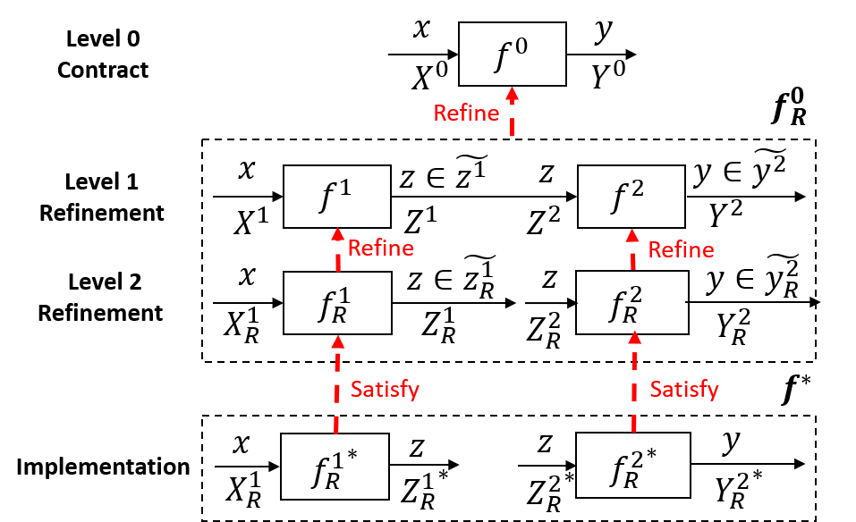
Figure 3: Refinement by decomposition takes a high-level contract and precisely reduces it to an implementation.

In general, requirement decomposition is to refine the requirements to the level that the sub-requirements are specific enough to build devices and integrate them to satisfy the top-level requirement. Fig. 3 is a simplified description of the process. The given Contract $f^{0}$ is decomposed into Subcontracts $f^{1}$ and $f^{2}$, which are further refined independently into $f^{1}_{R}$ and $f^{2}_{R}$; devices are then built independently by different suppliers to satisfy $f^{1}_{R}$ and $f^{2}_{R}$.

There are three tasks of the process:

• Primary refinement: $f^{1}$ and $f^{2}$ refine the higher-level Contract $f^{0}$ as a whole;

• Secondary refinement: the independently refined Contracts, $f^{1}_{R}$ and $f^{2}_{R}$, can refine $f^{0}$ as a whole;

• Satisfactory Implementation: given ${f^{1}_{R}}^{*}$ and ${f^{2}_{R}}^{*}$ satisfy $f^{1}_{R}$ and $f^{2}_{R}$ respectively, ${f^{1}_{R}}^{*}$ and ${f^{2}_{R}}^{*}$ can satisfy $f^{0}$ as a whole.

IV-B Reachability for primary refinement

Primary refinement means that the Level 1 refinement $f^{1}$ and $f^{2}$ as a whole (i.e. $f^{1}\wedge f^{2}$) have to refine $f^{0}$, as shown in Fig.12 (left). The right is an abstraction of $f^{1}$ and $f^{2}$ as a whole.

Figure 4: Primary Refinement

Primary refinement entails the following two requirements:

• The Subcontracts as a whole have to satisfy the refinement relationship:

  $$\forall x\in X^{0}:RA_{y}\subseteq\widetilde{y^{0}}$$

  $$X^{0}\subseteq X^{1},Y^{2}\subseteq Y^{0}$$

• The Subcontracts have to include the reachable sets of their respective variables:

  $$RA_{Y}\subseteq Y^{2},RA_{Z}\subseteq Z^{1},RA_{Z}\subseteq Z^{2}$$

Composability is irrelevant to the primary refinement. However, Composability is both sufficient and necessary for the secondary refinement and satisfactory Implementation.

IV-C Composability for satisfactory implementation

Proposition 1: If the Subcontracts of the primary refinement are composable and refined respectively by lower level Contracts, then the lower level Contracts are composable and can refine the given Contract as a whole.

The proof of Proposition 1 can be found in Appendix A. For the example process, Proposition 1 means if $f^{1}$ and $f^{2}$ are composable and can refine $f^{0}$ as a whole, and if $f^{1}_{R}$ and $f^{2}_{R}$ refine $f^{1}$ and $f^{2}$, then $f^{1}_{R}$ and $f^{2}_{R}$ are composable and can always refine $f^{0}$ as a whole. In other words, Composability in the primary refinement assures the secondary refinement and Composability between its Subcontracts.

Furthermore, Composability of the primary refinement is also a necessary condition for the secondary refinement. Refer to Appendix C for the proof.

Proposition 2: If the refined Subcontracts of a given Contract are composable and satisfied respectively by their Implementations, then the Implementations can satisfy the given Contract as a whole.

The proof of Proposition 2 can be found in Appendix B. For the example process, Proposition 2 means if $f^{1}_{R}$ and $f^{2}_{R}$ are composable and can refine $f^{0}$ as a whole, and if ${f^{1}_{R}}^{*}$ and ${f^{1}_{R}}^{*}$ satisfy $f^{1}_{R}$ and $f^{2}_{R}$ respectively, then ${f^{1}_{R}}^{*}$ and ${f^{1}_{R}}^{*}$ can refine $f^{0}$ as a whole. In other words, Composability in the secondary refinement assures a satisfying Implementation.

Combining Proposition 1 and 2, we can conclude that as long as the Subcontracts at all levels are composable and can refine their respective upper-level Contracts as a whole, the resulting Implementation are assured to satisfy the top-level Contract. Therefore, for the sub-requirements to be “correct”, they have to,

• satisfy the Contract formalism;

• be composable;

• refine the upper-level Contract as a whole.

These are the criteria for the correct-by-construction requirement decomposition.

V Automated Subcontracts definition

In this section, we will show how to use formal methods to automatically define Subcontracts that satisfy the “correctness” criteria.

V-A Design solution

Figure 5: An example design solution

The first step is to define a design solution. Architectural decomposition relies on the designer’s understanding of the desired system  [47] and thus is usually manually accomplished. The method to define the design solution is out the scope of this paper. Interested reader can refer  [48] for details.

Fig. 5 is an example design solution. Given Contract $f$, the design solution is comprised two Subcontracts: $f^{1}$ and $f^{2}$. The structure of the design solution can be captured by Fig.5 (right), and $f^{1}$ and $f^{2}$ are defined by $(x_{3},x_{4})^{T}=g^{1}(x_{1},x_{2},p_{1})$ and $x_{2}=g^{2}(x_{3},x_{4},p_{2})$ respectively, where $p_{1}\in P_{1}$ and $p_{2}\in P_{2}$. We further define $X_{i}^{k}$ is the bounded set for the variable $x_{j}$ of Subcontract $f^{k}$.

First, the design solution as a whole has to refine $f$, thus satisfying (8).

$$\forall x_{1}\in X_{1}^{0}:RA_{x_{2}}\subseteq\widetilde{x_{2}^{0}}$$

Second, the sets of the input variables have to be enlarged for refinement, but cannot be infinitely large. In our example, $X_{1}^{1}$ has to satisfy (9).

$$RA_{X_{2}}\subseteq X_{2}^{0}\text{ and }X_{1}^{0}\subseteq X^{1}_{1}$$

(8) and (9) are the requirements to decide the design solution and the refined input sets. If the given Contract is in Relational form, (8) is superceded by (9). If the given Contract is in Functional form, (8) should be proved by comparing the functional structures of the given Contract and the design solution. Most of the current verification-oriented works stop at this step [35].

Furthermore, it is crucial to separate the input from the parameter, e.g. separating $p_{1}$ from $x_{1}$ and $x_{2}$. While they both are independent variables of the functions, they are treated differently when refined. The size of the parameter set decreases as more knowledge is obtained at the later stage, but the size of the input set increases by the definition of refinement.

Finally, this specific example is selected only for illustration. The proposed methodology is applicable to any other general structure.

V-B The lower bound: Reachability Analysis

Subcontracts are used to develop devices independently so that when they are integrated together they can support the system operation as a whole. Therefore, the Subcontracts have to cover all the possible operation conditions based on the information available at the point of definition. Intuitively, the reachable sets represent all the possible operation condition, and hence they are the lower bound of the Subcontracts. Mathematically,

$$\text{If }X_{i}^{k}\neq\emptyset,RA_{X_{i}}\subseteq X_{i}^{k}$$

where $i\in\{1,2,3,4\}$ and $k\in\{1,2\}$.

In general, reachable sets can be calculated from reachability analysis. Adopted from  [49], the reachable set of this paper is defined as: for a given initial state $x(0)\in R^{n}$, $g$ is the system dynamic, $u(t)\in R^{m}$ is the system input at $t$, $u(\cdot)$ is the input trajectory, and $p\in R^{l}$ is a parameter vector. The continuous reachable set at time $t$ can be defined for a set of initial states $X(0)$, a set of uncertain time-varying external control $U(t)$, and a set of uncertain but fixed parameter values $P$, as

$$RA_{x}=\{g(x(0),u(\cdot),p)|x(0)\in X(0),u(t)\in U(t),p\in P\}.$$

where $RA_{x}\in R^{n}$ and $RA_{x_{i}}$ is the reachable set of $x_{i}$.

At this time, CORA  [49] is selected for the reachability analysis. CORA creates over-approximation of the theoretical reachable sets. There are more tools available to conduct reachability analysis such as  [50, 51, 52]. Better tools means tighter over-approximation. Detailed investigation among the available tools are planned for the future work.

V-C The upper bound: Constraint Programming

In theory, designers can always order the most capable devices of the market to build the system. However, the Subcontracts can never exceed suppliers’ realization capability, i.e. the realizable sets are the upper bound of the Subcontracts.

Typically, $f^{1}$ and $f^{2}$ are assigned to different suppliers for realization. Let $S_{i}^{k}$ be the realizable set of the ${x_{i}}$ for Subcontract $f^{k}$. Intuitively, it is impossible for the supplier to build anything that allows any inputs or accepts any outputs that are beyond the realizable sets. Therefore mathematically,

$$X_{i}^{k}\subseteq S_{i}^{k}$$

where $i\in\{1,2,3,4\}$ and $k\in\{1,2\}$.

In general, the realizable sets have to be consistent, i.e. conflict-free with each other. For example, if $S_{3}^{1}\cap S_{3}^{2}=\emptyset$, it means that the devices for $f^{1}$ and $f^{2}$ will not be compatible on variable $x_{3}$. Furthermore, if $S_{3}^{1}\cap S_{3}^{2}\neq\emptyset$, $S_{3}^{1}$ and $S_{3}^{2}$ will be contracted to $S_{3}^{1}\cap S_{3}^{2}$, which will be further propagated, contracting $X_{2}^{2}$. In the end, the contraction process propagate through all the functions until either the feasible space cannot be contracted anymore or an empty set is obtained.

Mathematically, the consistency among the realizable sets is a Constraint Satisfaction Problem (CSP)  [53]. A CSP is generally defined by a set of variables $\{x_{1},x_{2},..,x_{n}\}$; a set of domains $\{D_{1},D_{2},..,D_{n}\}$, such as for each variable $x_{i}$ , a domain $D_{i}$ with the possible values for that variable are given; and a set of constraints $\{C_{1},C_{2},..,C_{m}\}$, which are relations between the variables. Following the general formul ation of CSP, the example can be constructed as following. Note, $p_{1}$ and $p_{2}$ are uncertain parameters. They are not supposed to be contracted as the variables.

• Variables: $x_{i}$, where $i\in\{1,2,3,4\}$.

• Domains: $x_{i}\in S_{i}^{k}$, where $k\in\{1,2\}$

• Constraints: $g^{1}$ and $g^{2}$.

To check whether the realizable sets are consistent, the constraint propagation algorithms can be used. A constraint propagation algorithm iteratively reduces the domain of the variables, by using the set of constraints, until no domain can be contracted. At this point, Ibex  [54] is selected for the constraint programming. The classic HC4 algorithm  [55] is used as the contraction algorithm. There are more algorithms available to conduct constraint propagation  [56]. Different constraint propagation algorithms have different strength and weakness. Better algorithms contracts more infeasible space in shorter time. A detailed investigation among the available tools are planned for the future work.

As a result, the constraint programming algorithm outputs the contracted domain for each variable, denoted by $RE_{x_{i}}$. They are the upper bounds for the Subcontracts.

$$\text{If }X_{i}^{k}\neq\emptyset,X_{i}^{k}\subseteq RE_{x_{i}}$$

where $i\in\{1,2,3,4\}$ and $k\in\{1,2\}$.

V-D Trade-off study: Optimization

This step is to define the Subcontracts. Besides (10) and (11), (12-14) are the additional constraints between the Subcontracts: (12) is from the functional definition of the Subcontracts, (13) is from Composability and (14) is for the refinement of Contract $f$.

$$g^{1}((X_{1}^{1},X_{2}^{1})^{T},P_{1})\subseteq(X^{1}_{3},X^{1}_{4})^{T},$$

$$g^{2}((X^{2}_{3},X^{2}_{4})^{T},P_{2})\subseteq X^{2}_{2}.$$

$$X^{2}_{2}\subseteq X_{2}^{1},X^{1}_{3}\subseteq X^{2}_{3},X^{1}_{4}\subseteq X^{2}_{4}.$$

$$X^{2}_{2}\subseteq X_{2}^{0}$$

Therefore, (10-14) formulate the feasible space for the Subcontracts. To achieve the optimal Subcontracts, an objective function has to input manually depending on the specific goal. In the subsection, we will explain the tension between Subcontracts over the same variable and then use the tension to formulate the optimization problem as an example of trade-off study.

Figure 6: The inherent tension between Subcontracts.

$(X_{3}^{1},X_{4}^{1})$ and $(X_{3}^{2},X_{4}^{2})$ are bounded by the same lower bound and upper bound, as shown in Fig.6(a). Because $(x_{3},x_{4})$ is the output of $f^{1}$ and input of $f^{2}$. Therefore, the refinement of $(X_{3}^{1},X_{4}^{1})$ can only be selected from the orange area and the refinement of $(X_{3}^{2},X_{4}^{2})$ can only be selected from the green area. In other words, the bigger the white area is, the less choice of the secondary refinement has. Therefore, to maximize the available choices for the secondary refinement, $(X_{3}^{2},X_{4}^{2})=(X_{3}^{1},X_{4}^{1})$ has to be true. More generally, the Subcontracts over the same variable has to be the same. We denote the Subcontract over each variable $x_{i}$ as $X_{i}$, where $i\in\{1,2,3,4\}$. Therefore, the constraints in (10-14) can be rewritten and (15) is the new set of constraints for the Subcontracts, which always has to be satisfied regardless of the objective function selected for optimization.
$\begin{cases}RA_{X_{i}}\subseteq X_{i}\subseteq RE_{X_{i}}\\ g^{1}((X_{1},X_{2})^{T},P_{1})\subseteq(X_{3},X_{4})^{T}\\ g^{2}((X_{3},X_{4})^{T},P_{2})\subseteq X_{2}\\ X_{2}\subseteq X_{2}^{0}\end{cases}$        (15)

Furthermore, as shown in Fig.6(b), the closer $(X_{3},X_{4})$ is to the lower bound, the less options for $(X_{3}^{1},X_{4}^{1})$ to refine but the more options for $(X_{3}^{2},X_{4}^{2})$ and vice versa. Therefore, $(X_{3},X_{4})$ can neither too close to the upper bound nor to the lower bound. Based on this tension, we use barrier function to construct the objective function for the optimization. For any set $A$, let $\underline{A}$ denote the lower bound of $A$ and $\overline{A}$ denote the upper bound of $A$. Depending on the relationship between $x_{i}$ and $f^{k}$, which can be automatically derived from the structure (Fig.5), $h_{i}^{k}$ is defined as:
$h_{i}^{k}=\begin{cases}0:\text{ if }x_{i}\text{ is not connected to }f^{k}.\\ -a_{i}^{k}(\ln{|\overline{X_{i}}-\overline{RE_{x_{i}}}|+\ln{|\underline{X_{i}}-\underline{RE_{x_{i}}}|}}):\\ \text{if }x_{i}\text{ is the input of }f^{k}.\\ -a_{i}^{k}(\ln{|\overline{X_{i}}-\overline{RA_{x_{i}}}|+\ln{|\underline{X_{i}}-\underline{RA_{x_{i}}}|}}):\\ \text{if }x_{i}\text{ is the output of }f^{k}.\\ \end{cases}$
where $a_{i}^{k}$ is the realization difficulty coefficient with respect to the distance between the Subcontract and the upper and lower bounds.

Finally, therefore the objective function for the whole design solution is:

$$\text{min }\sum_{k=1}^{2}\sum_{i=1}^{4}h_{i}^{k}$$

$$s.t.(15)$$

V-E The semi-automated process

The semi-automated formal process for Subcontracts derivation is shown in Fig.7. The top level is the manual input; the middle level is the logic sequence that organizes the whole process; the bottom level are the formal methods that support the automatic computation of the conditions required by the middle level.

Figure 7: The overall scheme for automation

The process starts with the manual input of the design solution and the refined input set. First, (8) and (9) has to be automatically checked to see whether the design solution can refine the upper level requirement as a whole. If (8) is not satisfied, new design solution is required; if (9) is not satisfied, new refined input set needs to be manually selected. After (8) and (9) are satisfied, the lower bound of the Subcontracts, i.e. (10), are then decided using the reachable sets of all the variables identified in the reachability analysis.

Second, the realizable sets, i.e (11), are input to automatically compute the upper bound of the Subcontracts through constraint Programming. If no feasible solution can be found, it means there are conflicts in the realizable sets, which implies some supplier(s) is not compatible with others; if the contracted realizable sets fail to include their corresponding reachable sets, it implies some supplier(s) cannot provide the devices that the system operation requires.

Finally, optimization algorithms are applied to automatically find the optimal Subcontracts. The constraints, i.e. (15), can be automatically derived from (10-14) by the system. The objective function, i.e. (16), however has to be manually input depending the designer’s preference.

At this point, transition from step to step is still conducted manually. The interoperability between the tools still needs further investigation.

VI Case study: a cruise control example

We use the design of a cruise control system to illustrate the semi-automatic requirement decomposition process. The high level requirement is, for any initial speed between $v(0)\in[23.0,30.0]$ m/s and reference speed between $v_{ref}\in[34.5,35.5]$ m/s, the real speed shall be bounded by $v(t)\in[20,40]$ at all time (we simulated 100 seconds in this paper) and $v(t)\in[33.5,36.5]$ m/s after 20 seconds. The high level requirement is intentionally defined loosely for lower level refinement. Without the specific design detail available at the early stage, too strict requirement can be very difficult to realize.

We denote the Contract to be refined as $f^{0}$. Its input and output sets are defined as following. For any $(v_{ref},v(0))^{T}$ in the Input set, $v(t)$ has to be bounded by the Output set.

• Input of $f^{0}$:
  $v_{ref}\in[34.5,35.5]m/s$, $v(0)\in[23.0,30.0]m/s$.

• Output of $f^{0}$:
  $v(t)\in[20,40]m/s$, when $t\in[0,100]s$;
  $v(t)\in[33.5,36.5]m/s$, when $t\in[20,100]s$.

VI-A The design solution

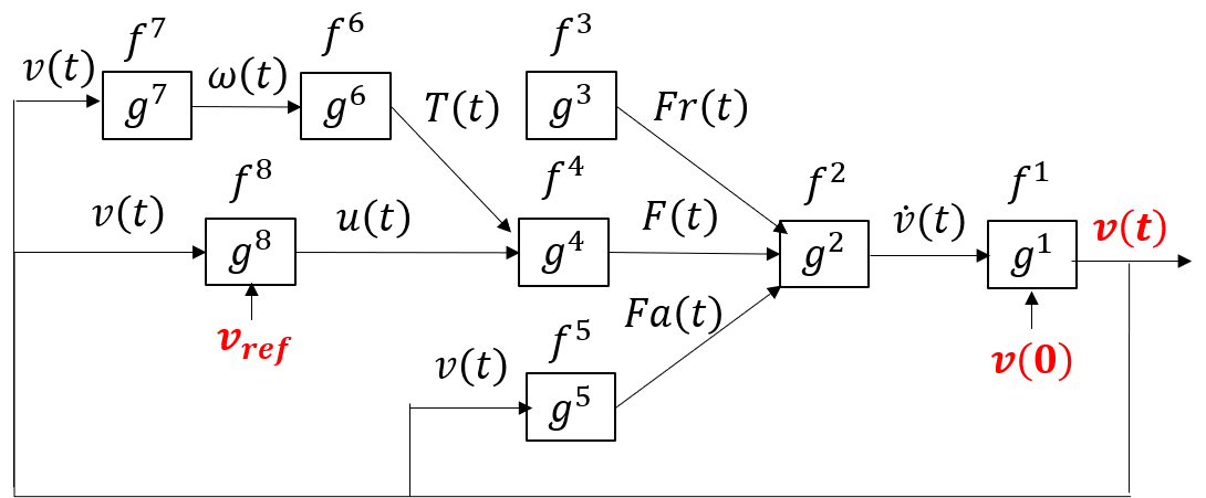
Figure 8: The design solution

Fig. 8 is a design solution of a cruise control system adopted from  [57]. The goal of this section is not to design the best cruise control system. We use the cruise control system to explain the requirement decomposition process. The design solution is comprised of 8 functions ($g^{1},g^{2},...,g^{8}$) as explained in Table I. 8 variables are also identified from the functions. $(v,\dot{v},Fr,F,Fa,T,\omega,u)^{T}=(x_{1},x_{2},...,x_{8})^{T}$. The uncertain parameters of the design solution are the total mass ($m$) and the maximal engine speed ($\omega_{m}$). Finally, the input sets are enlarged for the design solution to refine $f^{0}$.

$$v_{ref}\in[34.0,36.0]\text{ and }v(0)\in[22.0,30.0]$$

TABLE I: The functions of the design solution

$g^{i}$	Function	Explanation
$x_{1}=g^{1}(x_{2})$	$v(t)=\int_{0}^{t}\dot{v}dt+v(0)$	The definition of speed change
$x_{2}=g^{2}(x_{3},x_{4},x_{5},m)$	$\dot{v(t)}=(F(t)-Fr-Fa(t))/m$	The driving force $F(t)$, the aerodynamic drag $Fa(t)$ and the tyre friction $Fr$ are the force considered.
$x_{3}=g^{3}(m)$	$Fr=mgC_{r}$	The tyre friction, where $C_{R}$ is coefficient for the tyre friction.
$x_{4}=g^{4}(x_{6},x_{8})$	$F(t)=\alpha*u(t)T(t)$	The driving force, where $\alpha$ is the gear rate, $u(t)$ is the control input, $T(t)$ is the torque.
$x_{5}=g^{5}(x_{1})$	$Fa(t)=\frac{1}{2}\rho C_{d}Av(t)^{2}$	The aerodynamic drag, where $\rho$ is the air density, $C_{d}$ is the shape-dependent aerodynamic drag coefficient and $A$ is the frontal area of the car.
$x_{6}=g^{6}(x_{7},\omega_{m})$	$T(t)=T_{m}(1-\beta(\frac{\omega(t)}{\omega_{m}}-1)^{2})$	The torque is correlated to the engine speed $\omega(t)$ (RPM) and the maximum torque $T_{m}$ is obtained at engine speed $\omega_{m}$.
$x_{7}=g^{7}(x_{1})$	$\omega(t)=\alpha*v(t)$	The engine speed (RPM) is correlated with the car speed.
$x_{8}=g^{8}(x_{1})$	$u(t)=p(v_{ref}-v(t))+i\int_{0}^{t}(v_{ref}-v(t))dt$	The PI controller.
$x_{1}=v,x_{2}=\dot{v},x_{3}=F_{r},x_{4}=F,x_{5}=F_{a},x_{6}=T,x_{7}=\omega,x_{8}=u$
$m\in[900,1100],\omega_{m}\in[365,450],v_{ref}\in[34.0,36.0],v(0)\in[22.0,30.0],\alpha=10,g=9.8,C_{r}=0.01,C_{d}=0.32,\rho=1.3,A=2.4,\beta=0.4,T_{m}=200,p=0.1,i=0.5$

VI-B The Lower bound: reachable sets

Figure 9: Continuous evolution of the reachable sets of $(v(t),u(t))^{T}$ during $t\in[0,100]$

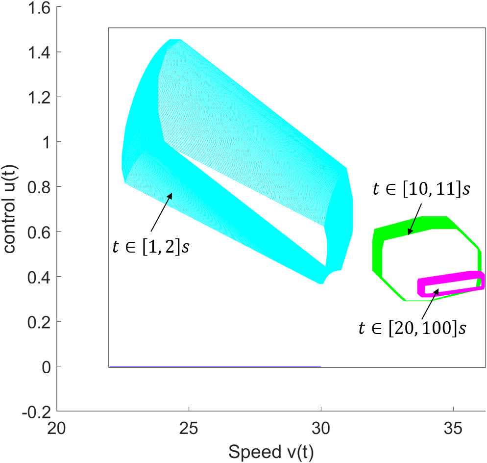
Figure 10: Discrete sampling of the reachable sets of $(v(t),u(t))^{T}$ during $t\in[0,100]$

CORA automatically computes the reachable sets of $(x_{1},x_{2},...,x_{8})$. Fig.9 is a continuous plot of the reachable set of $(v(t),u(t))^{T}$ for $t\in[0,100s]$. The blue line at the left bottom corner is the initial condition of $(v(0),u(0))^{T}$. It converges to the right and becomes stable at the darker red area as the time approaches to $t=100$. Fig. 10 shows the convergence of $(v(t),u(t))^{T}$ through time. In the beginning, it is bounded by the large blue area during $[1,2]s$; it then gradually migrates to the right and is bounded in the smaller green area for $[10,11]s$; during $[20,100]s$, it is bounded in the smallest magenta area. This discrete change in different sections of time coincides the narrowing and converging trend in Fig. 9. The reachable sets for the variables are listed in Table II.

TABLE II: The reachable sets during $t\in[0,100]$ seconds

Variable	Reachable set
$x_{1}=v(t)$	$[21.96649,36.22973]$
	$[33.65083,36.19185]$ for $t>20s$
$x_{2}=\dot{v(t)}$	$[-0.62937,2.89036]$
$x_{3}=Fr(t)$	$[88.20000,107.80000]$
$x_{4}=F(t)$	$[-9.33497,2997.78280]$
$x_{5}=Fa(t)$	$[240.87740,655.24649]$
$x_{6}=T(t)$	$[179.93903,200.00000]$
$x_{7}=\omega(t)$	$[219.66494,362.29727]$
$x_{8}=u(t)$	$[-0.00472,1.50660]$

First, $T(t)$ is bounded by $[179.93903,200.00000]$, which respects the maximum torque $T_{m}=200$; $\omega(t)$ is bounded by $[219.66494,362.29727]$, which respects the maximum engine speed bound $[365,450]$.

Second, as shown below, the output of the design solution is bounded by the output of the upper level Contract. (8) and (9) are satisfied and hence the proposed design solution can refine the upper level Contract as a whole. The reachable sets can be used as the lower bounds of the Subcontracts, and hence (10) is satisfied.

$$t\in[0,100]:v(t)\in[21.96649,36.22973]\subseteq[20.0,40.0]$$

$$t\in[20,100]:v(t)\in[33.65083,36.19185]\subseteq[33.5,36.5]$$

VI-C The upper bound: realizable sets

The design solution is then formulated into a CSP. Depending on the original sets, there are three possible types of results: (1) the original sets are successfully contracted and the contracted sets include the lower bounds, (2) the original sets are successfully contracted but the contracted sets do not include the lower bounds, (3) the original sets fails to be contracted, which implies internal conflicts among the original sets.

TABLE III: Test cases for the realizable sets

	Test 1	Test 2	Test 3
Variable	Original realizable sets
$x_{1}=v(t)$	[0,50]	[0,50]	[0,50]
$x_{2}=\dot{v(t)}$	[-1.5,3]	[-1.5,3]	[-1.5,3]
$x_{3}=Fr(t)$	[70,120]	[70,120]	[70,120]
$x_{4}=F(t)$	[-250,3500]	[-250,3500]	[-250,3500]
$x_{5}=Fa(t)$	[0,1000]	[0,1000]	[600, 1000]
$x_{6}=T(t)$	[0,250]	[0,180]	[0,180]
$x_{7}=\omega(t)$	[0,450]	[0,450]	[0,450]
$x_{8}=u(t)$	[-0.5,2]	[-0.5,2]	[-0.5,2]
Variable	Contracted realizable sets
$x_{1}=v(t)$	[0, 45.000]	[0, 33.000]	Empty
$x_{2}=\dot{v(t)}$	[-1.5, 3.0]	[-1.0, 3.0]
$x_{3}=Fr(t)$	[88.2,107.8]	[88.2, 107.8]
$x_{4}=F(t)$	[-250.0, 3500.0]	[-250,3500.0]
$x_{5}=Fa(t)$	[0,1000.0]	[0, 543.6]
$x_{6}=T(t)$	[120.0, 220.0]	[120.0, 180.0]
$x_{7}=\omega(t)$	[0,450.0]	[0,330.0]
$x_{8}=u(t)$	[-0.208, 2.0]	[-0.208, 2.0]

Table III are the test cases to show different types of possible results, where the original realizable sets are assumed the same for each variable of different blocks without losing generality. The original realizable sets in Test 1 are successfully contracted and the resulting sets are greater the lower bounds and hence can be the upper bounds for the Subcontracts. In Test 2, the realizable set of the torque $T(t)$ is changed to [0, 180]. The contracted sets of $v(t)$, $\omega(t)$, $T(t)$ and $Fa(t)$ fail to include the respective lower bounds. A new supplier that can provide larger torque range is suggested to replace the current one. In Test 3, the aerodynamic drag $Fa(t)$ is changed to [600,1000] compared with Test 2, and no feasible contracted realizable sets are available. Note that the contracted set of $Fa(t)$ in Test 2 is [0, 543.6]. It has no intersection with the original set of $Fa(t)$, [600,1000] in Test 3, which causes the internal conflict in Test 3.

The contracted realizable sets of Test 1 is adopted as the upper bounds for the Subcontracts and hence (11) is satisfied.

VI-D Trade-off study: optimal Subcontracts

We formulate the optimization problem, as shown in Table. IV, to achieve the optimal Subcontracts for the cruise control example. The decision variables are $\underline{X_{i}}$ and $\overline{X_{i}}$ denoting the lower bound and upper bound of the Subcontract $X_{i}$ ($i=1,2,...,8$). While the objective function depends on the designer’s preference, in this paper it is constructed following (16). The parameters to calculate $h_{i}^{k}$ can be found in Table. V. Furthermore, the constraints are constructed following (15), where $x=(x_{1}.x_{2},...,x_{8})^{T}$, $RA_{x_{i}}$ and $RE_{x_{i}}$ can be found in Table. V and $g^{i}$ can be found in Table. I.

TABLE IV: The optimization problem

Decision Variables	$\underline{X_{i}}$ and $\overline{X_{i}}$ where $i=1,2,...,8$
Objective Function	$\textit{min }\sum_{k=1}^{8}\sum_{i=1}^{8}h_{i}^{k}$
Constraints	$\overline{RA_{x_{i}}}\leq\overline{X_{i}}\leq\overline{RE_{x_{i}}}$ $\underline{RE_{x_{i}}}\leq\underline{X_{i}}\leq\underline{RA_{x_{i}}}$ $\underline{X_{1}}\geq 20,\overline{X_{1}}\leq 40$ $\underline{X_{7}}\leq g^{7}(\underline{X_{1}})$ $\overline{X_{7}}\geq g^{7}(\overline{X_{1}})$ $\underline{X_{6}}\leq g^{6}(\underline{X_{7}},\overline{\omega_{m}})$ $\overline{X_{6}}\geq g^{6}(\overline{X_{7}},\underline{\omega_{m}})$ $\underline{X_{5}}\leq g^{5}(\underline{X_{1}})$ $\overline{X_{5}}\geq g^{5}(\overline{X_{1}})$ $\underline{X_{4}}\leq g^{4}(\overline{X_{6}},\underline{X_{8}})$ $\overline{X_{4}}\geq g^{4}(\overline{X_{6}},\overline{X_{8}})$ $\underline{X_{2}}\leq g^{2}(\underline{X_{4}},\overline{X_{3}},\overline{X_{5}},\overline{m})$ $\overline{X_{2}}\geq g^{2}(\overline{X_{4}},\underline{X_{3}},\underline{X_{5}},\underline{m})$ $\underline{\omega_{m}}=365,\overline{\omega_{m}}=450,\underline{m}=900,\overline{m}=1100$

TABLE V: The parameters for the trade-off study

$X_{i}$	$[\underline{RA_{x_{i}}},\overline{RA_{x_{i}}}]$	$[\underline{RE_{x_{i}}},\overline{RE_{x_{i}}}]$	Difficulty coefficients
$X_{1}$	$[22.00,36.23]$	$[0,45]$	$a_{1}^{1}=0.9,a_{1}^{5}=0.5$, $a_{1}^{7}=0.1,a_{1}^{8}=0.8$
$X_{2}$	$[-0.63,2.89]$	$[-1.5,3.0]$	$a_{2}^{1}=0.6,a_{2}^{2}=0.6$
$X_{3}$	$[88.20,107.80]$	$[88.2,107.8]$	$a_{3}^{3}=0.5,a_{3}^{2}=0.4$
$X_{4}$	$[-9.36,2997.78]$	$[-250.0,3500.0]$	$a_{4}^{4}=0.3,a_{4}^{2}=0.8$
$X_{5}$	$[240.88,655.25]$	$[0,1000.0]$	$a_{5}^{5}=0.4,a_{5}^{2}=0.7$
$X_{6}$	$[179.94,200.00]$	$[120.0,220.0]$	$a_{6}^{6}=0.1,a_{2}^{2}=0.9$
$X_{7}$	$[219.67,362.30]$	$[0,450.0]$	$a_{7}^{7}=0.5,a_{7}^{6}=0.6$
$X_{8}$	$[-0.005,1.51]$	$[-0.29,2.0]$	$a_{8}^{8}=0.9,a_{8}^{4}=0.9$

The resulting optimal Subcontracts are shown in Table. VI. The given Contract (i.e. Level 0) is refined by the second row, and the Subcontracts (i.e. the decomposed requirements) are in the third row.

Note that $u$ is added to Level 0, and $f^{1}$ and $f^{8}$ do not appear in the Level 1 Subcontracts. The reason is that the speed $v$ and the control input $u$ are system property and hence cannot be assigned to lower level. More specifically, take $f^{1}$ for example. On one hand, given $\dot{v(t)}$, nothing about $v(t)$ can be reasoned without knowing the evolution history of $\dot{v(t)}$ from 0 to $t$, which is in fact determined by the composition of the whole system. On the other hand, $v(t)$ can be reasoned at Level 0 with respect to the input of $v(0)$ and $v_{ref}$. This means $v(t)$ belongs to Level 0 and can only be guaranteed by Level 0. This is also the reason that $g^{1}$ and $g^{8}$ are not the constraints of the optimization problem in Table. IV.

TABLE VI: The optimal Subcontracts

		Input	Output
Level 0 Contract		$v_{ref}\in[34.5,35.5]$ $v(0)\in[22.0,30.0]$	$v\in[20,40]$
Level 0 Refinement		$v_{ref}\in[34.0,36.0]$ $v(0)\in[22.0,30.0]$	$v\in[21.8,38.4]$ $u\in[-0.1,1.511]$
Level 1 Subcontract	$f^{2}$	$Fr\in[88.2,107.8]$ $F\in[-159.1,3024.0]$ $F_{a}\in[237.6,827.6]$	$\dot{v}\in[-1.1,3]$
	$f^{3}$	NA	$Fr\in[88.2,107.8]$
	$f^{4}$	$T\in[150,200.1]$ $u\in[-0.1,1.511]$	$F\in[-159.1,3024.0]$
	$f^{5}$	$v\in[21.8,38.4]$	$F_{a}\in[237.6,827.6]$
	$f^{6}$	$\omega\in[109.8,406.1]$	$T\in[150,200.1]$
	$f^{7}$	$v\in[21.8,38.4]$	$\omega\in[109.8,406.1]$

VII Conclusion

In this paper, we propose a formal approach for semi-automatic requirement decomposition. Compared with the large volume of current work on the (bottom-up) compositional verification, this framework focuses on the top-down sub-requirement generation and mathematically guarantee their correctness by construction. To achieve this, we developed a formalism for requirement definition and correctness criteria for requirement decomposition. Together, they facilitate a step-wise hierarchical refinement process that can be further automated by the well-supported formal methods, such as Reachability Analysis and Constraint Programming. The process was then formulated to be readily solved by the aforementioned formal methods for practitioner friendly requirement decomposition and analysis. Lastly, a case study was conducted on a cruise control example to detail the specific steps of the requirement generation process and demonstrate the effectiveness of the proposed approach.

A limitation of this work is that not all the requirements can be represented by a continuous bounded set. Many systems are more accurately modeled as transition systems, which deal with discrete traces. We expect the methodology to apply to the transition systems and will demonstrate it on concrete examples in the future.

Appendix A Proof of Proposition 1

Proof: Fig. 11 is the atomic form of Contract refinement. Proposition 1 means, $f^{1}$ and $f^{2}$ are composable and refine $f^{0}$ as a whole, if $f^{1}_{R}$ refines $f^{1}$ and $f^{2}_{R}$ refines $f^{2}$ independently, then secondary refinement is guaranteed, i.e. $f^{1}_{R}$ and $f^{2}_{R}$ as a whole can always refine $f$.

First, we prove $f^{1}_{R}$ and $f^{2}_{R}$ are composable.
$f^{1}$ and $f^{2}$ are composable $\Longrightarrow Z^{1}\subseteq Z^{2}$;
$f^{1}_{R}$ and $f^{2}_{R}$ refine $f^{1}$ and $f^{2}$ respectively $\Longrightarrow Z^{1}_{R}\subseteq Z^{1}$ and $Z^{2}\subseteq Z^{2}_{R}$;
Therefore, $Z^{1}_{R}\subseteq Z^{2}_{R}$ and thus $f^{1}_{R}$ and $f^{2}_{R}$ are composable.

Second, we prove $f^{1}_{R}$ and $f^{2}_{R}$ as a whole can refine $f^{0}$.
Level 1 Contract refines Level 2 Contract $\Longrightarrow x\in X^{0}:f^{2}(f^{1}(x))\subseteq\widetilde{y^{0}}$. Meanwhile, $f^{1}_{R}$ refines $f^{1}$ $\Longrightarrow x\in X^{1}:\widetilde{z^{1}_{R}}\subseteq f^{1}(x)$. Furthermore, because $f^{2}_{R}$ refines $f^{2}$, hence $x\in X^{1}:f^{2}_{R}(\widetilde{z^{1}_{R}})\subseteq f^{2}(f^{1}(x))$. Hence, $x\in X^{1}:f^{2}_{R}(\widetilde{z^{1}_{R}})\subseteq f^{2}(f^{1}(x))\subseteq\widetilde{y^{0}}$. Because $X^{0}\subseteq X^{1}$, therefore $x\in X^{0},f^{2}_{R}(\widetilde{z^{1}_{R}})\subseteq\widetilde{y^{0}}$ and hence (7-1) is satisfied.
$f^{1}_{R}$ and $f^{2}_{R}$ refine $f^{1}$ and $f^{2}$ respectively $\Longrightarrow X^{1}\subseteq X^{1}_{R}$ and $Y^{2}_{R}\subseteq Y^{2}$, hence (7-2) is satisfied.
All the possible values of $z$ are included by $Z_{R}^{1}$ and all the possible values of $y$ are included by $Y_{R}^{2}$. Therefore, at the second level, $RA_{Z}\subseteq Z_{R}^{1}\subseteq Z_{R}^{2}$ and $RA_{Y}\subseteq Y_{R}^{2}$. Hence, (7-3) is satisfied.

Therefore, $f^{1}_{R}$ and $f^{2}_{R}$ refine $f^{0}$ as a whole. $\blacksquare$

Figure 11: Secondary refinement

Appendix B Proof of Proposition 2

Proof: Fig. 12 is the atomic form of satisfaction by refinement. Proposition 2 means, if Subcontracts $f^{1}$ and $f^{2}$ are composable and refine $f^{0}$, then the Implementation ${f^{1}}^{*}$ and ${f^{2}}^{*}$ are composable and when composed together, they satisfy Contract $f^{0}$.

First, we prove ${f^{1}}^{*}$ and ${f^{2}}^{*}$ are composable.
Contract $f^{1}$ and $f^{2}$ are composable $\Longrightarrow Z^{1}\subseteq Z^{2}$.
${f^{1}}^{*}$ satisfies $f^{1}$ $\Longrightarrow{Z^{1}}^{*}\subseteq Z^{1}$ .
Therefore, ${Z^{1}}^{*}\subseteq Z^{2}$ holds and hence Implementation ${f^{1}}^{*}$ and ${f^{2}}^{*}$ are composable.

Second, we prove ${f^{1}}^{*}$ and ${f^{1}}^{*}$ as a whole satisfy $f^{0}$.
$f^{1}$ and $f^{2}$ refine $f^{0}$ as a whole $\Longrightarrow x\in X^{0}:f^{2}(f^{1}(x))\subseteq\widetilde{y^{0}}$.
${f^{1}}^{*}$ satisfies $f^{1}\Longrightarrow x\in X^{1}:{f^{1}}^{*}(x)\in f^{1}(x)$.
${f^{2}}^{*}$ satisfies $f^{2}\Longrightarrow x\in X^{1}:{f^{2}}^{*}({f^{1}}^{*}(x))\in f^{2}(f^{1}(x)).$
Because $X^{0}\subseteq X^{1}$, therefore $x\in X^{0}:{f^{2}}^{*}({f^{1}}^{*}(x))\in f^{2}(f^{1}(x))\subseteq\widetilde{y^{0}}$ and hence ${f^{1}}^{*}$ and ${f^{1}}^{*}$ as a whole satisfy $f^{0}$. $\blacksquare$

Figure 12: Composable Subcontracts for Implementation

Appendix C

In this section, we prove Composability is also a necessary condition.

Proposition 3: As shown in Fig. 11, given $f^{1}_{R}$ refines $f^{1}$ and $f^{2}_{R}$ refines $f^{2}$ independently, $f^{1}$ and $f^{2}$ have to be composable otherwise $f^{1}_{R}$ and $f^{2}_{R}$ can fail to refine $f^{1}$ and $f^{2}$ as a whole.

Proof: Because $f^{1}$ and $f^{2}$ are refined independently, hence any feasible refinement $f^{1}_{R}$ and $f^{2}_{R}$ should be able to refine $f^{0}$ as a whole. We prove by contradiction here to show if $f^{1}$ and $f^{2}$ are not composable, $f^{1}_{R}$ and $f^{2}_{R}$ might fail to refine $f^{0}$.
At Level 1, assuming $Z^{2}\subseteq Z^{1}$, hence $RA^{1}_{Z}\subseteq Z^{2}\subseteq Z^{1}$.
At Level 2, assuming $f^{2}_{R}=f^{2}$, hence $Z^{2}_{R}=Z^{2}$.
Because $X^{1}\subseteq X^{1}_{R}$, it is possible that $RA^{1}_{Z}\subseteq Z^{2}\subseteq RA^{2}_{Z}$.
If this is the case, then $Z^{2}_{R}\subseteq RA^{2}_{Z}$, contradicting (7-3).

If $f^{1}$ and $f^{2}$ are not composable, the independently refined Subcontracts might fail to refine $f^{0}$ as a whole. Therefore, Composability in the primary refinement is also a necessary condition for the secondary refinement. $\blacksquare$

References

- [1] S. J. Kapurch, NASA systems engineering handbook. Diane Publishing, 2010.
- [2] ANSI/EIA, “Processes for engineering a system,” Electronic Industries Alliance, 1999.
- [3] D. L. Lempia and S. P. Miller, “Requirements engineering management handbook,” National Technical Information Service (NTIS), vol. 1, 2009.
- [4] D. P. Kirkman, “Requirement decomposition and traceability,” Requirements Engineering, vol. 3, no. 2, pp. 107–114, 1998.
- [5] P. Braun, M. Broy, F. Houdek, M. Kirchmayr, M. Müller, B. Penzenstadler, K. Pohl, and T. Weyer, “Guiding requirements engineering for software-intensive embedded systems in the automotive industry,” Computer Science-Research and Development, vol. 29, no. 1, pp. 21–43, 2014.
- [6] C. Baier and J.-P. Katoen, Principles of model checking. MIT press, 2008.
- [7] K. Lundqvist, “Introducing Formal Methods,” https://web.mit.edu/16.35/www/lecturenotes/FormalMethods.pdf, 2002, [Online; accessed 19-August-2019].
- [8] D. Greising and J. Johnsson, “Behind Boeing’s 787 delays,” https://www.buffalo.edu/content/dam/www/news/imported/pdf/December07/ChicagoTribPritchardBoeing.pdf, 2007, [Online; accessed 19-August-2019].
- [9] G. Le Lann, “An analysis of the ariane 5 flight 501 failure-a system engineering perspective,” in Proceedings International Conference and Workshop on Engineering of Computer-Based Systems. IEEE, 1997, pp. 339–346.
- [10] S. Wagner, D. M. Fernández, M. Felderer, A. Vetrò, M. Kalinowski, R. Wieringa, D. Pfahl, T. Conte, M.-T. Christiansson, D. Greer et al., “Status quo in requirements engineering: A theory and a global family of surveys,” ACM Transactions on Software Engineering and Methodology (TOSEM), vol. 28, no. 2, p. 9, 2019.
- [11] B. Penzenstadler, “Desyre-decomposition of systems and their requirements,” Ph.D. dissertation, Technische Universität München, 2011.
- [12] SAE, “Guidelines for development of civil aircraft and systems,” SAE International, 2010.
- [13] M. Abbasipour, “A framework for requirements decomposition, sla management and dynamic system reconfiguration,” Ph.D. dissertation, Concordia University, 2018.
- [14] P. W. Melancon, “Categorization and representation of functional decomposition by experts,” NAVAL POSTGRADUATE SCHOOL MONTEREY CA, Tech. Rep., 2008.
- [15] A. S. Sidky, R. R. Sud, S. Bhatia, and J. D. Arthur, “Problem identification and decomposition within the requirements generation process,” Department of Computer Science, Virginia Polytechnic Institute & State …, Tech. Rep., 2002.
- [16] K. G. Salter, “A methodology for decomposing system requirements into data processing requirements,” in Proceedings of the 2nd international conference on Software engineering. IEEE Computer Society Press, 1976, pp. 91–101.
- [17] A. P. Moore, “The specification and verified decomposition of system requirements using csp,” IEEE Transactions on Software Engineering, vol. 16, no. 9, pp. 932–948, 1990.
- [18] IEEE guide for developing system requirements specifications. IEEE, 1998.
- [19] IEEE recommended practice for software requirements specifications, IEEE Std-830 (1998). IEEE, 1998.
- [20] C. Arora, M. Sabetzadeh, L. C. Briand, and F. Zimmer, “Requirement boilerplates: Transition from manually-enforced to automatically-verifiable natural language patterns,” in 2014 IEEE 4th International Workshop on Requirements Patterns (RePa). IEEE, 2014, pp. 1–8.
- [21] P. Mahendra and A. Ghazarian, “Patterns in the requirements engineering: A survey and analysis study,” WSEAS Transaction on Information Science and Application, vol. 11, 2014.
- [22] P. Reinkemeier, I. Stierand, P. Rehkop, and S. Henkler, “A pattern-based requirement specification language: Mapping automotive specific timing requirements,” Software Engineering 2011–Workshopband, 2011.
- [23] A. Rajan and T. Wahl, CESAR-cost-efficient methods and processes for safety-relevant embedded systems. Springer, 2013, no. 978-3709113868.
- [24] P. H. Feiler, D. P. Gluch, and J. J. Hudak, “The architecture analysis & design language (aadl): An introduction,” Carnegie-Mellon Univ Pittsburgh PA Software Engineering Inst, Tech. Rep., 2006.
- [25] H. Lönn and U. Freund, “Automotive architecture description languages,” in Automotive Embedded Systems Handbook. CRC Press, 2017, pp. 9–1.
- [26] M. Bozzano, A. Cimatti, J.-P. Katoen, V. Y. Nguyen, T. Noll, M. Roveri, and R. Wimmer, “A model checker for aadl,” in International Conference on Computer Aided Verification. Springer, 2010, pp. 562–565.
- [27] K. Hu, T. Zhang, Z. Yang, and W.-T. Tsai, “Exploring aadl verification tool through model transformation,” Journal of Systems Architecture, vol. 61, no. 3-4, pp. 141–156, 2015.
- [28] A. Johnsen, K. Lundqvist, P. Pettersson, and O. Jaradat, “Automated verification of aadl-specifications using uppaal,” in 2012 IEEE 14th International Symposium on High-Assurance Systems Engineering. IEEE, 2012, pp. 130–138.
- [29] V. Debruyne, F. Simonot-Lion, and Y. Trinquet, “East-adl—an architecture description language,” in IFIP World Computer Congress, TC 2. Springer, 2004, pp. 181–195.
- [30] J.-R. Abrial, M. Butler, S. Hallerstede, T. S. Hoang, F. Mehta, and L. Voisin, “Rodin: an open toolset for modelling and reasoning in event-b,” International journal on software tools for technology transfer, vol. 12, no. 6, pp. 447–466, 2010.
- [31] T. Gibson-Robinson, P. Armstrong, A. Boulgakov, and A. Roscoe, “FDR3 — A Modern Refinement Checker for CSP,” in Tools and Algorithms for the Construction and Analysis of Systems, ser. Lecture Notes in Computer Science, E. Ábrahám and K. Havelund, Eds., vol. 8413, 2014, pp. 187–201.
- [32] A. Benveniste, B. Caillaud, D. Nickovic, R. Passerone, J.-B. Raclet, P. Reinkemeier, A. Sangiovanni-Vincentelli, W. Damm, T. Henzinger, and K. G. Larsen, “Contracts for system design,” 2012.
- [33] A. Benveniste, W. Damm, A. Sangiovanni-Vincentelli, D. Nickovic, R. Passerone, and P. Reinkemeier, “Contracts for the design of embedded systems part i: Methodology and use cases,” Contract, vol. 2, p. G1, 2012.
- [34] A. Benveniste, B. Caillaud, D. Nickovic, R. Passerone, J.-B. Raclet, P. Reinkemeier, A. Sangiovanni-Vincentelli, W. Damm, T. A. Henzinger, K. G. Larsen et al., “Contracts for system design,” Foundations and Trends® in Electronic Design Automation, vol. 12, no. 2-3, pp. 124–400, 2018.
- [35] A. Sangiovanni-Vincentelli, W. Damm, and R. Passerone, “Taming dr. frankenstein: Contract-based design for cyber-physical systems,” European journal of control, vol. 18, no. 3, pp. 217–238, 2012.
- [36] L. Benvenuti, A. Ferrari, L. Mangeruca, E. Mazzi, R. Passerone, and C. Sofronis, “A contract-based formalism for the specification of heterogeneous systems,” in 2008 Forum on Specification, Verification and Design Languages. IEEE, 2008, pp. 142–147.
- [37] W. Damm, H. Hungar, B. Josko, T. Peikenkamp, and I. Stierand, “Using contract-based component specifications for virtual integration testing and architecture design,” in 2011 Design, Automation & Test in Europe. IEEE, 2011, pp. 1–6.
- [38] A. Cimatti and S. Tonetta, “A property-based proof system for contract-based design,” in 2012 38th Euromicro Conference on Software Engineering and Advanced Applications. IEEE, 2012, pp. 21–28.
- [39] D. Cofer, A. Gacek, S. Miller, M. W. Whalen, B. LaValley, and L. Sha, “Compositional verification of architectural models,” in NASA Formal Methods Symposium. Springer, 2012, pp. 126–140.
- [40] J.-B. Raclet, E. Badouel, A. Benveniste, B. Caillaud, A. Legay, and R. Passerone, “A modal interface theory for component-based design,” Fundamenta Informaticae, vol. 108, no. 1-2, pp. 119–149, 2011.
- [41] A. Cimatti, M. Dorigatti, and S. Tonetta, “Ocra: A tool for checking the refinement of temporal contracts,” in 2013 28th IEEE/ACM International Conference on Automated Software Engineering (ASE). IEEE, 2013, pp. 702–705.
- [42] A. Benveniste, B. Caillaud, D. Nickovic, R. Passerone, J.-B. Raclet, P. Reinkemeier, A. Sangiovanni-Vincentelli, W. Damm, T. Henzinger, and K. G. Larsen, “Contracts for systems design: methodology and application cases,” 2015.
- [43] J. Iber, A. Höller, T. Rauter, and C. Kreiner, “Towards a generic modeling language for contract-based design.” in ModComp@ MoDELS, 2015, pp. 24–29.
- [44] M. D. Mesarovic, D. Macko, and Y. Takahara, Theory of hierarchical, multilevel, systems. Elsevier, 2000, vol. 68.
- [45] A. Kusiak and N. Larson, “Decomposition and Representation Methods in Mechanical Design,” Journal of Mechanical Design, vol. 117, no. B, pp. 17–24, 06 1995. [Online]. Available: https://doi.org/10.1115/1.2836453
- [46] K. Ye, S. Foster, and J. Woodcock, “Compositional assume-guarantee reasoning of control law diagrams using utp,” in From Astrophysics to Unconventional Computation. Springer, 2020, pp. 215–254.
- [47] A. Benveniste, B. Caillaud, D. Nickovic, R. Passerone, J.-B. Raclet, P. Reinkemeier, A. Sangiovanni-Vincentelli, W. Damm, T. Henzinger, and K. G. Larsen, “Contracts for systems design: Theory,” 2015.
- [48] H. Komoto and T. Tomiyama, “A theory of decomposition in system architecting,” in DS 68-2: Proceedings of the 18th International Conference on Engineering Design (ICED 11), Impacting Society through Engineering Design, Vol. 2: Design Theory and Research Methodology, Lyngby/Copenhagen, Denmark, 15.-19.08. 2011, 2011.
- [49] M. Althoff, “Cora 2016 manual,” Technische Universitat Munchen, Garching, Germany, 2016.
- [50] L. Benvenuti, D. Bresolin, A. Casagrande, P. Collins, A. Ferrari, E. Mazzi, A. Sangiovanni-Vincentelli, and T. Villa, “Reachability computation for hybrid systems with ariadne,” IFAC Proceedings Volumes, vol. 41, no. 2, pp. 8960–8965, 2008.
- [51] P.-J. Meyer, A. Devonport, and M. Arcak, “Tira: toolbox for interval reachability analysis,” in Proceedings of the 22nd ACM International Conference on Hybrid Systems: Computation and Control. ACM, 2019, pp. 224–229.
- [52] S. Bogomolov, M. Forets, G. Frehse, K. Potomkin, and C. Schilling, “Juliareach: a toolbox for set-based reachability,” in Proceedings of the 22nd ACM International Conference on Hybrid Systems: Computation and Control. ACM, 2019, pp. 39–44.
- [53] F. Rossi, P. Van Beek, and T. Walsh, Handbook of constraint programming. Elsevier, 2006.
- [54] G. Chabert, “Ibex documentation,” 2018.
- [55] F. Benhamou, F. Goualard, L. Granvilliers, and J.-F. Puget, “Revising hull and box consistency,” in Int. Conf. on Logic Programming. Citeseer, 1999.
- [56] I. Kueviakoe, A. Lambert, P. Tarroux et al., “Comparison of interval constraint propagation algorithms for vehicle localization,” Journal of Software Engineering and Applications, vol. 5, no. 12, p. 157, 2013.
- [57] K. J. Aström and R. M. Murray, Feedback systems: an introduction for scientists and engineers. Princeton university press, 2010.