A simple supergravity model of inflation constrained with Planck 2018 data

Abstract

We study a model of inflation based on $\mathcal{N}=1$ supergravity essentially depending on one effective parameter. Under a field transformation we show that this model turns out to be equivalent to a previously studied supergravity model known to be ruled out with the original choice of the parameter. Such parameter measures the slope of the potential at observable scales. Through a Bayesian parameter estimation, it is shown how this model is compatible with recent CMB temperature measurements by Planck 2018 giving rise to a simple, viable, single field model of inflation. The tensor to scalar ratio constraint is found to be $r_{0.002}<0.065$ with negative running. We discuss how observables are invariant under the field transformation which leaves unaltered the slow-roll parameters. As a consequence the use of one presentation of the model or its field-transformed version is purely a matter of convenience.

I Introduction

The inflationary paradigm has proved its validity against early universe observables which are detected with ever-higher precision by modern experiments. Most prominently, the latest data release of the Planck Satellite [1] reports, for instance, a spectrum of primordial scalar fluctuations with index $n_{s}=0.965\pm 0.004$, perfectly consistent with a standard slow-roll inflation model [2]. Several realizations of inflation offer a link between this paradigm and fundamental physics of the early universe and/or a good fit to data, mostly in terms of a single canonical scalar field dubbed the inflaton [3] (and see [4] for a plethora of viable models). A common exercise is the search for characteristic signatures to discriminate between distinct models (potentials). The recent constrain to the tensor-to-scalar ratio $r$ [5] rejects several of the models of inflation which feature large values of this parameter ([2], and see [6] for a generic characteristic of inflationary potentials resulting in large $r$). In this context, symmetries of the slow-roll parameters are here employed to group apparently different potentials in a single description and thus reduce the number of models to test by observations. This may provide physical foundation for empirical models. In this paper, we study a model rooted in supergravity which essentially depends on one parameter identified with the slope of the potential during the inflationary era. The value of this parameter is fixed by means of a Bayesian analysis resulting in a viable model. We discuss two interpretations of the possible origin of the inflationary epoch suggested by the very location of the potential. In the first presentation of the model given by Eq. (9) and Fig. 2 we naturally interpret inflation as a transient phenomenon with the inflaton rolling from high energy and starting inflation somewhere at $\eta=1$ and ending when $\eta=-1$ (in this model $\epsilon$ is always less than $|\eta|)$. A total number of $e$-folds can be quantified containing the necessary number of $e$-folds for observable inflation. A field transformation can take this potential (without any deformation) to the one given by Eq. (14) and Fig. 3 making easier to obtain approximated expressions for quantities of interest. As discussed long time ago [7, *Nanopoulos:1982bv, *Ovrut:1983my, *Holman:1984yj, 11] it is then natural to interpret the second presentation of this model as originating from a previous phase transition from a high energy symmetric potential where thermal effects keep the inflaton initially at the origin, afterwards slowly rolling towards its global minimum. In both cases the observables are exactly the same because the potential has not been deformed by the field transformation. Physically relevant quantities like the spectral index, tensor to scalar ratio and all other observables do not depend on the particular value of $\phi_{H}$ but only when referred to a specific potential. The potential an all its even-number of derivatives are unchanged by the operations of translation and reflection but odd-number of derivatives of the potential switch sign (because of the $\phi\rightarrow-\phi$ transformation). However the slow-roll (SR) parameters remain unchanged since they involve an even number of factors with odd-number of derivatives of the potential. As a consequence observables remain the same as shown in the body of the article. The outline of the paper is as follows: in Section II we provide a brief presentation of the supergravity model by writing the Kähler potential and the superpotential thus specifying the F-term part of the scalar potential. Section III contains a brief discussion of the slow-roll parameters and their invariance under the field redefinition. In Section IV we choose a convenient version of the model where analytical approximations can be easily done. Section V contains a Bayesian analysis for the estimation of parameter values which best fit the Planck 2018 data. Finally Section VI contains a brief discussion of the main results and conclusions.

II A supergravity model of inflation

The piece of the $\mathcal{N}=1$ supergravity model of interest is given by the action [12]

$$I=-\int d^{4}x\sqrt{-g}\left(\frac{1}{2}R+G_{i}^{\,\,j}\partial_{\mu}\Phi^{i}\partial_{\nu}\Phi^{*}_{j}g^{\mu\nu}+V\right),$$ (1)

where the Kähler metric $G_{i}^{\,\,j}$ is defined by $G_{i}^{\,\,j}=\partial^{2}G/\left(\partial\Phi^{*}_{j}\partial\Phi^{i}\right)$ and the Kähler function is $G(\Phi^{i},\Phi^{*}_{i})=K(\Phi^{i},\Phi^{*}_{i})+\ln|W(\Phi^{i})|^{2}$, $W$ is a holomorphic function of $\Phi^{i}$ called superpotential and $K$ is the Kähler potential, a real function depending on the superfields $\Phi^{i}$ as well as their conjugates $\Phi^{*}_{i}$. The $F-term$ part of the scalar potential is given in terms of the real function $G$ as follows

$$V=e^{G}\left(G_{i}(G^{-1})^{i}_{j}G^{j}-3\right).$$ (2)

In what follows we concentrate in a single chiral superfield $\Phi$ with scalar component $z$. Thus, the potential is given by

$$V=e^{K}\left(F_{z}(K_{zz^{*}})^{-1}F^{*}_{z^{*}}-3|W|^{2}\right),$$ (3)

where

$$F_{z}\equiv\frac{\partial W}{\partial z}+\frac{\partial K}{\partial z}W,\quad K_{zz^{*}}\equiv\frac{\partial^{2}K}{\partial z\partial z^{*}}.$$ (4)

To first approximation we take the Kähler potential to be of the canonical form

$$K(z,z^{*})=(z-z_{0})(z^{*}-z^{*}_{0})+\cdot\cdot\cdot\,,$$ (5)

with superpotential

$$W(z)=f(z_{0})z^{2},$$ (6)

where $f(z_{0})$ is a constant with dimensions of mass which we simple take as $\Lambda$. The scalar potential becomes

$$V=\Lambda^{2}e^{|z-z_{0}|^{2}}|z|^{2}\left(-3|z|^{2}+|2+|z|^{2}-z_{0}z^{*}|^{2}\right).$$ (7)

Writing $z$ in terms of real components

$$z=\frac{1}{\sqrt{2}}(\phi+i\chi),$$ (8)

we find that the $\chi$-direction is a stable direction of the full potential, shown in Fig. 1.

Figure 1: The full potential given by Eqs. (7) and (8) along the $\chi$ and $\phi$ directions. The $\chi$ direction is stable and we can then study the inflationary $\phi$-direction safely on its own.

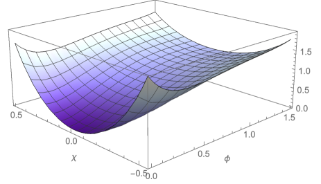
Thus we set $\chi=\chi_{0}=0$ and study the potential along the inflationary $\phi$-direction only which is given by

$$V=\frac{1}{8}\Lambda^{2}e^{\frac{1}{2}(\phi-\phi_{0})^{2}}\left(16\phi^{2}-8\phi_{0}\phi^{3}+(2+\phi^{2}_{0})\phi^{4}\right.\\ \left.-2\phi_{0}\phi^{5}+\phi^{6}\right).$$ (9)

This potential is illustrated in Fig. 2 for some typical values of the parameters. We see that the potential given by Eq. (9) has a minimum at $\phi=0$ with vanishing energy.

Figure 2: Schematic plot of the inflationary potential given by Eq. (9). Here, the inflaton rolls towards it global minimum (conveniently located at the origin) and inflation is a transient phenomenon with a finite total number of $e$-folds. We can locate the beginning of inflation at $\eta=1$ and its end when $\eta=-1$ with the parameter $\epsilon$ always smaller than $|\eta|.$ A fit to the Planck-2018 data suggest the the total number of $e$-folds is no more than triple the usually required 60 $e$-folds of observable inflation. In its form given by Eq. (9) the resulting potential is somewhat reminiscent of Starobinsky’s but with a different asymptotic behavior.

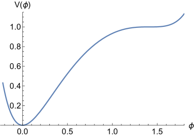
For $\phi=\phi_{0}$ the derivative of the potential is

$$V^{\prime}=\frac{1}{2}\Lambda^{2}\phi_{0}(8-4\phi_{0}^{2}),$$ (10)

thus, the potential is also flat for $\phi_{0}=\sqrt{2}\,.$ To make further analytical progress we would have to find $\phi_{H}$ perhaps through an expansion of the spectral index for $\phi-\phi_{0}$ small. Equivalently we can can shift the origin away from the minimum at $\phi=0$ and make a reflection around the new origin i.e., by making the field transformation $\phi\rightarrow-\phi+\phi_{0}$. In terms of the original field $z$ we have that $z\rightarrow-z+z_{0}$ then

$$K(z,z^{*})\rightarrow zz^{*}+\cdot\cdot\cdot\,,$$ (11)

with superpotential [7, *Nanopoulos:1982bv, *Ovrut:1983my, *Holman:1984yj, 11]

$$W(z)\rightarrow\Lambda(z-z_{0})^{2},$$ (12)

the resulting potential is given by

$$V=\Lambda^{2}e^{zz^{*}}(z-z_{0})(z^{*}-z^{*}_{0})\left[4+z^{*}(z+z_{0}+z(z-z_{0})z^{*})+(z-3z_{0}-z^{2}z^{*}+zz^{*}z_{0})z^{*}_{0}\right].$$ (13)

Parameterising as in Eq. (8) we set the stable direction $\chi=\chi_{0}=0$ and study the potential along the inflationary $\phi$-direction only [7, *Nanopoulos:1982bv, *Ovrut:1983my, *Holman:1984yj, 11, 13]

$$V=\Lambda^{2}e^{\frac{1}{2}\phi^{2}}(\phi-\phi_{0})^{2}\left[2+\frac{1}{8}(\phi-\phi_{0})\left(6\phi_{0}+\phi(2+\phi^{2}-\phi\phi_{0})\right)\right].$$ (14)

This potential is illustrated in Fig. 3 for some typical values of the parameters. This form of the potential can be viewed as an example of inflection point inflation. Such type of models have been studied in e.g., [14, 15], in the context of the Minimal Supersymetric Standard Model (MSSN). There, the particular $A$-term in the inflationary potential (also known as $A-$term inflation [16]) can induce a saddle point at which $V^{\prime}(\phi=0)=V^{\prime\prime}(\phi=0)=0$. While this fails to reproduce an acceptable $n_{s}$ [17, 18], a point of inflection with non-zero $V^{\prime}(\phi=0)$ can successfully do so, as we show explicitly for our case in Sec. IV.

In our case, we see that the potential of Fig. 3 is exactly of the same shape as the one shown by Fig. 2 but looked at from a different frame. The potential has not been deformed, i.e., it has only been displaced and reflected. Thus, all observables calculated from the potential Eq. (14) should take exactly the same values as the ones calculated from Eq. (9). The new SR parameters have the same values when evaluated at the new $\phi_{H}$ as the old SR parameters had when evaluated at the old $\phi_{H}$.

Figure 3: Schematic plot of the inflationary potential given by Eq. (14). The minimum occurs for $\phi=\phi_{0}$ and the potential is flat at the origin if $\phi_{0}=\sqrt{2}$. Here we use Planck-2018 data to fix the slope at the origin. The fact that a viable model (according to Planck-2018 data) does not require $V^{\prime}=0$ at the origin makes us to abandon the idea that the potential (14) originates from a phase transition from a high energy symmetric potential where thermal effects keep the inflaton initially at the origin. Instead we propose that it would be more natural to think in a potential not committed with developing inflation close to the origin. Although both potentials are equivalent (since they give the same observables), the potential given by Eq. (9) and Fig. 2 does not suggest that the origin is privileged in any way being inflation a transient phenomenon where both the beginning and end to inflation can be found and a total number of $e$-folds can be quantified. For calculations, however, we find more convenient to work with Eq. (14) and we stick to this presentation of the potential in what follows.

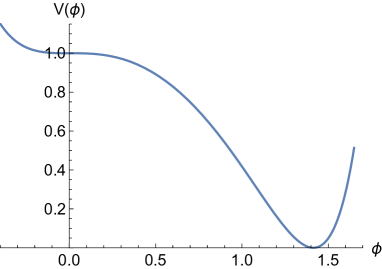
This shows explicitly how physically relevant quantities like the spectral index, tensor to scalar ratio and all other observables do not depend on the frame in which the potential is evaluated. These features are discussed in detail in the next section.

III Slow-roll parameters and observables

The potential an all its even-number of derivatives are unchanged by the operations of translation and reflection but odd-number of derivatives of the potential change sign (because $\phi\rightarrow-\phi$ was used). However the SR parameters remain unchanged since they involve an even number of factors with odd-number of derivatives of the potential. In slow-roll inflation, the spectral indices are given in terms of the slow-roll parameters of the model, these are given by (see e.g. [19, 20, *Liddle:2000cg])

$$\epsilon\equiv\frac{M^{2}}{2}\left(\frac{V^{\prime}}{V}\right)^{2},\quad\eta\equiv M^{2}\frac{V^{\prime\prime}}{V},\\ \xi_{2}\equiv M^{4}\frac{V^{\prime}V^{\prime\prime\prime}}{V^{2}},\quad\xi_{3}\equiv M^{6}\frac{V^{\prime 2}V^{\prime\prime\prime\prime}}{V^{3}}.$$ (15)

Here primes denote derivatives with respect to the inflaton $\phi$ and $M$ is the reduced Planck mass $M=2.44\times 10^{18}\,\mathrm{GeV}$ which we set $M=1$ in most of what follows. For the case at hand all the SR parameters are given by complicated expressions which are functions of the potential $V(\phi)$ and its derivatives an are not reproduced here. Thus, the SR parameters are given in terms of the potential $V(\phi)$ and its derivatives. Because when going from the old potential Eq. (9) to the new one Eq. (14) the potential has not been locally changed and because odd number of derivative terms appear always in even numbers in the SR parameters then it follows that the observables remain unchanged. The potential as given by Eq. (9) and Fig. 2 seems more natural than that of Eq. (14) and Fig. 3 since it does not suggest that inflation is somehow connected with a previous phase transition from a symmetric phase at high energy where the inflaton is originally kept by thermal effects at the origin.

The primordial power spectra $\mathcal{P}_{i}$, a power-law parameterized spectra of scalar and tensor perturbations, is usually given in terms of the spectral amplitude $A_{i}$ and the spectral indices $n_{i}$, where the subindex _i refers to either scalar $(s)$ or tensor $(t)$ components

$$\mathcal{P}_{s}(k) = A_{s}\left(\frac{k}{k_{H}}\right)^{(n_{s}-1)},$$ (16)

$$\mathcal{P}_{t}(k) = A_{t}\left(\frac{k}{k_{H}}\right)^{n_{t}}=rA_{s}\left(\frac{k}{k_{H}}\right)^{n_{t}},$$ (17)

where $k$ is the wave number and $r\equiv\mathcal{P}_{t}(k)/\mathcal{P}_{s}(k)$ the ratio of tensor to scalar perturbations at pivot scale $k=k_{H}$, here set to $k_{H}=0.002\mathrm{Mpc}^{-1}$ [22, 23, 24]. Slow-roll inflation predicts the spectrum of curvature perturbations to be close to scale-invariant (for a review of cosmic inflation and its relationship with cosmological observations see [22]). This allows a simpler parameterization of the spectra in terms of quantities evaluated at $k_{H}$ such as the spectral index, the running, and even the running of the running of scalar perturbations [25]

$$\mathcal{P}_{s}(k) = A_{s}\left(\frac{k}{k_{H}}\right)^{(n_{s}-1)+\frac{1}{2}n_{sk}\ln\left(\frac{k}{k_{H}}\right)+\frac{1}{6}n_{skk}\left(\ln\left(\frac{k}{k_{H}}\right)\right)^{2}},$$ (18)

$$\mathcal{P}_{t}(k) = A_{t}\left(\frac{k}{k_{H}}\right)^{n_{t}+\frac{1}{2}n_{tk}\ln\left(\frac{k}{k_{H}}\right)},$$ (19)

where $n_{tk}$ is the running of the tensor index $n_{t}$, $n_{sk}$ the running of the scalar index $n_{s}$ in a self-explanatory notation. In the slow-roll approximation these observables are given by (see e.g. [19, 20, *Liddle:2000cg, 23, 24])

$$n_{t} = -2\epsilon=-\frac{r}{8},$$ (20)

$$n_{s} = 1+2\eta-6\epsilon,$$ (21)

$$n_{tk} = \frac{dn_{t}}{d\ln k}=4\epsilon\left(\eta-2\epsilon\right)=\frac{r}{64}\left(r-8(1-n_{s})\right),$$ (22)

$$n_{sk} = \frac{dn_{s}}{d\ln k}=16\epsilon\eta-24\epsilon^{2}-2\xi_{2},$$ (23)

$$A_{s}(k) = \frac{1}{24\pi^{2}}\frac{\Lambda^{4}}{\epsilon_{H}},$$ (24)

where the amplitude of density perturbations at wave number $k$ is $A_{s}(k)$ and the scale of inflation is $\Lambda$, with $\Lambda\equiv V_{H}^{1/4}$.

IV Choosing a convenient version of the model

For calculations we find more convenient to work with Eq. (14) and we stick to this presentation of the potential in what follows. We see that the potential given by Eq. (14) has now a minimum at $\phi_{0}$ with vanishing energy. We redefine $\phi_{0}$ in terms of a new parameter $s$ as follows

$$\phi_{0}=s/8+\sqrt{2},$$ (25)

and calculate the derivative of $V$ at the origin

$$V^{\prime}(\phi=0)/\Lambda^{2}=s+\frac{3s^{2}}{16\sqrt{2}}+\frac{s^{3}}{256}.$$ (26)

Thus $s$ measures the slope of the potential at the origin. Previous works [7, *Nanopoulos:1982bv, *Ovrut:1983my, *Holman:1984yj, 11] take $s=0$ giving a model presently ruled out by the data [18]. Given that there is no special reason (apart from simplicity) to fix $V^{\prime}(\phi)=0$ at the origin. We perform a Bayesian parameter fitting to determine the value of $s$ (and consequently $\phi_{0}$), consistent with Planck 2018 data set. In this way the value of $\phi_{0}$ turns out to be very close to $\sqrt{2}$ resulting in a viable model. The simplifying assumption $V^{\prime}(\phi=0)=0$ is typically motivated by the suggestion that thermal effects at higher energy put the inflaton at the origin and then a phase transition makes the inflaton rolls to its global minimum. This view is partially motivated by the privileged position given to the origin. In the equivalent potential of Eq. (9) and Fig. 2 no such interpretation seems to arise because the origin does not play any particular rol during inflation. We take the view, in any case, that the scalar field starts rolling from high energies to the global minimum of the potential and that an epoch of inflation occurs without any need for the inflaton to start its rolling from a privileged point. Thus, in this scheme, inflation is a transient phenomenon which consequently lasts a measurable finite ${\it total}$ number of $e$-folds. In this case both the start and the end of inflation localized in field space by the conditions $|\eta|=1$. Having said so, the potential and its observables can be studied using the frame which results more convenient for the calculation at hand keeping in mind that the displacement away from the origin is irrelevant. Thus, in what follows we study the potential as given by Eq. (14) and we extract an approximate formula for $\phi_{H}$. At $\phi=0$ the derivative of the potential Ec. (14) is given by $V^{\prime}\left(\phi=0\right)=-\frac{1}{2}\Lambda^{2}\phi_{0}\left(8-4\phi^{2}_{0}\right)$ thus, $\phi_{0}=\sqrt{2}$ is a flat direction of the potential. As a consequence $\phi_{H}$ should be close to the origin and we can obtain an approximate value for it by a simple expansion of the spectral index around $\phi=0$. The result is

$$\phi_{H}^{new}\approx\frac{1}{39}\left(6\sqrt{2}-\sqrt{33+39n_{s}}\right)\approx\frac{1}{12\sqrt{2}}\left(1-n_{s}\right).$$ (27)

Making $\phi_{H}\rightarrow-\phi_{H}+\phi_{0}$ we obtain an approximated expression for $\phi_{H}$ for the old potential of Eq. (9).

$$\phi_{H}^{old}\approx\frac{1}{39}\left(33\sqrt{2}+\sqrt{33+39n_{s}}\right)\approx\frac{1}{12\sqrt{2}}\left(23+n_{s}\right).$$ (28)

Using the central value reported by Planck 2018 $n_{s}\approx 0.9649$ we find $\phi_{H}^{new}\approx 0.00206$ while $\phi_{H}^{old}\approx 1.41216$. This simple result makes explicitly clear that the value of the field is not relevant per se since the observables are the same whether we use $\phi_{H}^{new}\approx 0.00206$ in the new potential or $\phi_{H}^{old}\approx 1.41216$ in the old one. Also, the model defined by Eq. (14) and illustrated by Fig. 3 has a $\Delta\phi$ of exactly the same size as in the old potential given by Eq. (9). The end of inflation is here given by the condition $\eta=-1$ being $\epsilon$ much smaller than one during the whole period of inflation. It is convenient to use the ”new” version of the potential given by Eq. (14) and initially assume $\phi_{0}=\sqrt{2}$ since $\eta$ does not change appreciably for small changes in $\phi_{0}$. Also, the number of $e$-folds is not really sensitive to small changes in $\phi$ at the end of inflation and a numerical estimate of $\phi_{e}$ yields a good approximation, however, extreme care should be taken for $\phi$ close to $\phi_{H}$. Thus, the solution to $\eta=-1$ when $\phi_{0}=\sqrt{2}$ is given by $\phi_{e}\approx 0.1694$. For the ”new” potential $\phi_{H}$ should be close to the origin and we can obtain an approximate value for it by a simple expansion of the spectral index around $\phi=0$. We should expect that the number of $e$-folds close to $\phi_{H}$ is sensitive to changes in $\phi_{H}$. Because $\phi_{H}$ depends on $\phi_{0}$ and $\phi_{0}$ weakly depends on $s$ we use Eq. (25) and also expand in $s$. The result, to first order in $s$ is

$$\phi_{H}^{new}\approx\frac{2-3\sqrt{2}\,s-2n_{s}}{24\sqrt{2}+9s},$$ (29)

which reduces to Eq. (27) when $s=0$. We then find the parameter $s$ by requiring that the number of $e$-folds from $\phi_{H}$ to $\phi_{e}$ is a certain number, let us say $N=60$. The number of $e$-folds from $\phi_{H}$ to the end of inflation at $\phi_{e}$ is given by

$$N\equiv-\int_{\phi_{H}}^{\phi_{e}}\frac{V({\phi})}{V^{\prime}({\phi})}{d}{\phi}.$$ (30)

Table 1: Observables obtained with the value $s=-8.3\times 10^{-5}$, equivalently $\phi_{0}=1.414203.$ This value of $s$ is first obtained from the requirement of $60$ $e$-folds of inflation using the central value for the spectral index $n_{s}=0.9649$ through Eqs. (29) and (30).

$\phi_{0}$	$N$	$r$	$n_{s}$	$n_{sk}$	$\Lambda$ (GeV)
1.414203	$60$	$8.2\times 10^{-8}$	$0.9649$	$1.7\times 10^{-3}$	$5.5\times 10^{14}$

We find that $s\approx-8.3\times 10^{-5}$ thus, the required slope of the potential at the origin is small indeed. The value of $s$, which controls $V^{\prime}$ at the origin (see Eq. (26)), turns out to be only a small correction to the value of $\phi_{0}$. As proved in the following sections, this is not unexpected as $V^{\prime}$ at the inflection point cannot be too large in order to obtain values of $n_{s}$ consistent with CMB observations. This fine-tuning issue of inflection point inflation has also been discussed in the context of MSSN $A-$term inflation in [14, 15]. Here we rely on the Bayesian treatment of data to determine the acceptable values of $s$. This is a relevant issue since, while the small value of $s$ does not appreciably change $\phi_{H}$ it is crucial in the estimation of $N$, given that $V^{\prime}({\phi})$ appears in Eq. (30) is proportional to $s$. The beginning of inflation is here given by the SR condition $\eta=1$ which occurs for $\phi_{b}\approx-0.09442$ giving a total number of $e$-folds $N_{T}=163$. Thus, inflation is here only a transient phenomenon lasting almost thrice the required 60 $e$-folds. Observables obtained with this value for $s$ are given in Table 1.

V Analysis of the model in light of Planck 2018 data

Even though the primary parameters that describe the CMB spectrum have already been tightly constrained in several inflationary models and have little impact on the $B$-mode spectrum, it is worthwhile to perform a full parameter-space exploration to determine the tensor-to-scalar ratio constraints for the model. Throughout this model, we assume purely Gaussian adiabatic scalar and tensor contributions with a flat $\Lambda$CDM background specified by the standard parameters (see Table 2): the physical baryon ($\Omega_{\rm b}h^{2}$) and cold dark matter density ($\Omega_{\rm c}h^{2}$) relative to the critical density ($h$ is the dimensionless Hubble parameter such that $H_{0}=100h$ kms^-1Mpc^-1), $\theta$ being $100\times$ the ratio of the sound horizon to angular diameter distance at last scattering surface and $\tau$ denotes the optical depth at reionization. We consider the tensor-to-scalar ratio defined previously as $r\equiv\mathcal{P}_{t}(k)/\mathcal{P}_{s}(k)$, and hereafter we set the ratio $r=r(k_{H})$ at a scale of $k_{H}=0.002{\rm Mpc^{-1}}$. The parameters describing the primordial spectrum for the model along with its flat priors imposed in our Bayesian analysis are shown in Table 2; see [26, 27] and references therein for a Bayesian description over the primordial spectrum.

Throughout the analysis, the $C_{\ell}$’s spectra – temperature and polarization (E & B) – are computed with a modified version of the CAMB code [28], and the parameter estimation is performed using the CosmoMC program [29]. To compute posterior probabilities for each model we use the full-mission Planck 2015 observations of temperature and polarization anisotropies of the CMB radiation (PLK; [30]) and the B-mode polarization constraints from a joint analysis analysis of BICEP2, Keck Array, and Planck (BKP; [31]) data. Furthermore, we use Baryon acoustic oscillations data to break parameter degeneracies from CMB measurements (BAO; [32] and references therein). We refer to this combined dataset as Dataset I. Similarly, to incorporate the up-to-date version of the data we include the full-mission Planck 2018 (TT,TE,EE+lowE+lensing) [1], the Keck Array and BICEP2 Collaborations 2016 [5] and the BAO data [32], named as Dataset II.

Table 2: Parameters and prior ranges used in our analysis. Last four columns display mean values along with 1-$\sigma$ estimation. For one-tailed distributions the upper limit 95% CL is given. For two-tailed the 68% is shown. Derived parameters are labeled with ^∗.

Parameter	Prior range	Dataset I	Dataset II	Dataset I	Dataset II
[0.1cm] $\Omega_{\rm b}h^{2}$	[0.01, 0.03]	$0.02231\pm 0.00014$	$0.02242\pm 0.00013$	$0.02230\pm 0.00020$	$0.02242\pm 0.00018$
$\Omega_{\rm DM}h^{2}$	[0.01 , 0.3]	$0.1185\pm 0.0010$	$0.11946\pm 0.0009$	$0.1185\pm 0.0015$	$0.1194\pm 0.0012$
$\theta$	[1.0 , 1.1]	$1.04088\pm 0.00029$	$1.04098\pm 0.00029$	$1.04085\pm 0.00043$	$1.04099\pm 0.00039$
$\tau$	[0.01 , 0.3]	$0.078\pm 0.014$	$0.057\pm 0.007$	$0.078\pm 0.020$	$0.057\pm 0.010$
$\log[10^{10}A_{\rm s}]$	[2.5 , 4.0]	$3.089\pm 0.027$	$3.049\pm 0.014$	$3.088\pm 0.039$	$3.050\pm 0.020$
$\phi_{0}$ [1.414 –]	[190 , 210]	$202\pm 1.3$	$202\pm 1.1$	$202\pm 5.6$	$200\pm 4.8$
$r_{02}$	[ 0 , 0.5]	$<0.078$	$<0.065$	$<0.106$	$<0.921$
$N$	[30 , 90]	$60$	60	$63.2\pm 11.7$	$58.5\pm 8.3$
${}^{*}n_{s}$	-	$0.9670\pm 0.0042$	$0.9661\pm 0.0037$	$0.9670\pm 0.0058$	$0.9661\pm 0.0052$
${}^{*}n_{sk}$	-	$-0.0018\pm 0.0001$	$-0.0017\pm 0.00009$	$-0.0017\pm 0.0007$	$-0.0020\pm 0.0006$
${}^{*}n_{tk}[10^{-10}]$	-	$-3.758\pm 0.070$	$-3.770\pm 0.047$	$-4.508\pm 3.821$	$-5.476\pm 3.552$

Figure 4: 2D probability posterior distributions for the power spectrum Sugra model parameters ($N=60$); 2D constraints are plotted with $1\sigma$ and $2\sigma$ confidence contours.

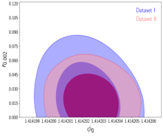
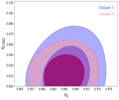
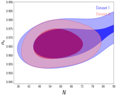
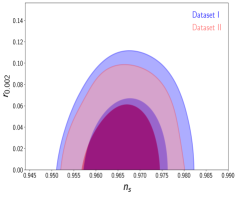
Table 2 summarizes the observational constraints of the parameters that describe the model (as well as the derived parameters, labelled by ^∗). Figure 4 displays 2D marginalized posterior distributions of the parameters used to describe the model along to Dataset I (blue) and Dataset II (red). A similar analysis is performed when the $e$-fold number $N$ is considered as an extra free quantity (shown in Figure 5). The inner ellipses show the 68% confidence region, and the outer edges the 95% region.

Figure 5: 2D probability posterior distributions for the power spectrum Sugra model parameters letting the $e$-fold number be a free parameter. 2D constraints are plotted with $1\sigma$ and $2\sigma$ confidence contours.

The Dataset II, considering $N=60$ constrains the parameter of the model as $\phi_{0}=1.414202\pm 1.1\times 10^{-6}$ at 68 $\%$ C.L., and $r<0.065$ at 95 $\%$ C.L., which can be mapped into $n_{s}=0.9661\pm 0.0037$, in agreement with Planck 2018 observations, with the addition of a negative running of the spectral index $n_{sk}=-0.0017\pm 0.00009$. Moreover, the updated information allows to tighten the constraints on the $e$-fold parameter such as $N=58.5\pm 8.3$ in agreement with the initial assumptions made in Table 1.

VI Discussion of Results and Conclusions

In this paper we presented a model of inflation derived from an $\mathcal{N}=1$ supergravity realization, taking advantage of the stable direction and interpreting the dynamical part as the inflaton with a transit slow-roll period. We have exploited the mirror-shift symmetry of the slow-roll parameters (and the slow-roll inflation observables) to displace the vacuum away from the origin at $\phi=0$ and represent the potential as in Eq. (14), plotted in Fig. 3. Approximated, analytic expressions are easier to find here as compared with the original potential given by Eq. (9). Through a Bayesian parameter fitting we have determined the range of values for $\phi_{0}$ compatible with the latest Planck 2018 data, as well as the predicted spectral index and tensor-to-scalar ratio. As shown in Fig. 4, the value $\phi_{0}=\sqrt{2}$ is ruled out by more than three standard deviations but we have shown that the supergravity model is flexible enough to accommodate values away from this reference value.

The results confirm our analytical assumption of $N=60$ consistent with Planck 2018 data; in the upper panel of Fig. 5, the number of $e$-folds is constrained to a finite range of values centered around $N=58.5$. This is an important feature of the model. It stems from the transient aspect of the inflationary phase. Moreover, for a given total number of $e$-folds, our inflationary model admits only specific values of the equation of state during the reheating stage, consistent with observed spectral index values [33].

References

- [1] N. Aghanim et al. Planck 2018 results. VI. Cosmological parameters. 2018, astro-ph/1807.06209.
- [2] Y. Akrami et al. Planck 2018 results. X. Constraints on inflation. 2018, astro-ph/1807.06211.
- [3] Alan H. Guth. The Inflationary Universe: A Possible Solution to the Horizon and Flatness Problems. Phys. Rev., D23:347–356, 1981. [Adv. Ser. Astrophys. Cosmol.3,139(1987)].
- [4] Jerome Martin, Christophe Ringeval, and Vincent Vennin. Encyclopædia Inflationaris. Phys. Dark Univ., 5-6:75–235, 2014, astro-ph/1303.3787.
- [5] P. A. R. Ade et al. Improved Constraints on Cosmology and Foregrounds from BICEP2 and Keck Array Cosmic Microwave Background Data with Inclusion of 95 GHz Band. Phys. Rev. Lett., 116:031302, 2016, astro-ph/1510.09217.
- [6] Gabriel Germán, Alfredo Herrera-Aguilar, Juan Carlos Hidalgo, and Roberto A. Sussman. Canonical single field slow-roll inflation with a non-monotonic tensor-to-scalar ratio. JCAP, 1605(05):025, 2016, astro-ph/1512.03105.
- [7] John R. Ellis, Dimitri V. Nanopoulos, Keith A. Olive, and K. Tamvakis. Fluctuations in a Supersymmetric Inflationary Universe. Phys. Lett., 120B:331–334, 1983.
- [8] Dimitri V. Nanopoulos, Keith A. Olive, M. Srednicki, and K. Tamvakis. Primordial Inflation in Simple Supergravity. Phys. Lett., 123B:41–44, 1983.
- [9] Burt A. Ovrut and Paul J. Steinhardt. Supersymmetry and Inflation: A New Approach. Phys. Lett., 133B:161–168, 1983.
- [10] R. Holman, Pierre Ramond, and Graham G. Ross. Supersymmetric Inflationary Cosmology. Phys. Lett., 137B:343–347, 1984.
- [11] Graham G. Ross and Subir Sarkar. Successful supersymmetric inflation. Nucl. Phys., B461:597–624, 1996, hep-ph/9506283.
- [12] E. Cremmer, S. Ferrara, L. Girardello, and Antoine Van Proeyen. Yang-Mills Theories with Local Supersymmetry: Lagrangian, Transformation Laws and SuperHiggs Effect. Nucl. Phys., B212:413, 1983. [413(1982)].
- [13] G. German and Axel de la Macorra. A Model of inflation independent of the initial conditions, with bounded number of e-folds and n(s) larger or smaller than one. Phys. Rev., D70:103521, 2004, astro-ph/0410133.
- [14] J. C. Bueno Sanchez, Konstantinos Dimopoulos, and David H. Lyth. A-term inflation and the MSSM. JCAP, 0701:015, 2007, hep-ph/0608299.
- [15] Rouzbeh Allahverdi, Kari Enqvist, Juan Garcia-Bellido, Asko Jokinen, and Anupam Mazumdar. MSSM flat direction inflation: Slow roll, stability, fine tunning and reheating. JCAP, 0706:019, 2007, hep-ph/0610134.
- [16] David H. Lyth. MSSM inflation. JCAP, 0704:006, 2007, hep-ph/0605283.
- [17] Rouzbeh Allahverdi, Kari Enqvist, Juan Garcia-Bellido, and Anupam Mazumdar. Gauge invariant MSSM inflaton. Phys. Rev. Lett., 97:191304, 2006, hep-ph/0605035.
- [18] Cláudio Gomes, Orfeu Bertolami, and João G. Rosa. Inflation with data: A survey of some exotic inflationary models. Phys. Rev., D97(10):104061, 2018, hep-th/1803.08084.
- [19] Andrew R. Liddle, Paul Parsons, and John D. Barrow. Formalizing the slow roll approximation in inflation. Phys. Rev., D50:7222–7232, 1994, astro-ph/9408015.
- [20] David H. Lyth and Antonio Riotto. Particle physics models of inflation and the cosmological density perturbation. Phys. Rept., 314:1–146, 1999, hep-ph/9807278.
- [21] Andrew R. Liddle and D. H. Lyth. Cosmological inflation and large scale structure. 2000.
- [22] J. Alberto Vázquez, Luis E. Padilla, and Tonatiuh Matos. Inflationary Cosmology: From Theory to Observations. 2018, astro-ph/1810.09934.
- [23] P. A. R. Ade et al. Planck 2013 results. XXII. Constraints on inflation. Astron. Astrophys., 571:A22, 2014, astro-ph/1303.5082.
- [24] P. A. R. Ade et al. Planck 2015 results. XX. Constraints on inflation. Astron. Astrophys., 594:A20, 2016, astro-ph/1502.02114.
- [25] Brian A. Powell. Scalar runnings and a test of slow roll from CMB distortions. 2012, astro-ph/1209.2024.
- [26] J. Alberto Vazquez, A. N. Lasenby, M. Bridges, and M. P. Hobson. A Bayesian study of the primordial power spectrum from a novel closed universe model. Mon. Not. Roy. Astron. Soc., 422:1948–1956, 2012, astro-ph/1103.4619.
- [27] J. Alberto Vazquez, M. Bridges, M. P. Hobson, and A. N. Lasenby. Model selection applied to reconstruction of the Primordial Power Spectrum. JCAP, 1206:006, 2012, astro-ph/1203.1252.
- [28] Antony Lewis, Anthony Challinor, and Anthony Lasenby. Efficient computation of CMB anisotropies in closed FRW models. Astrophys. J., 538:473–476, 2000, astro-ph/9911177.
- [29] Antony Lewis and Sarah Bridle. Cosmological parameters from CMB and other data: A Monte Carlo approach. Phys. Rev., D66:103511, 2002, astro-ph/0205436.
- [30] P. A. R. Ade et al. Planck 2015 results. XIII. Cosmological parameters. Astron. Astrophys., 594:A13, 2016, astro-ph/1502.01589.
- [31] P. A. R. Ade et al. Joint Analysis of BICEP2/ and Data. Phys. Rev. Lett., 114:101301, 2015, astro-ph/1502.00612.
- [32] Lauren Anderson et al. The clustering of galaxies in the SDSS-III Baryon Oscillation Spectroscopic Survey: baryon acoustic oscillations in the Data Releases 10 and 11 Galaxy samples. Mon. Not. Roy. Astron. Soc., 441(1):24–62, 2014, astro-ph/1312.4877.
- [33] Gabriel German, Juan Carlos Hidalgo, and Ariadna Montiel. Work in progress, 2019.