Lyra’s cosmology of homogeneous and isotropic universe in Brans-Dicke theory

Abstract

In this paper, we investigate a scalar field Brans-Dicke cosmological model in Lyra’s geometry which is based on the modifications in geometrical term as well as energy term of Einstein’s field equations. We have examined the validity of proposed cosmological model on observational scale by performing statistical analysis from latest $H(z)$ and SN Ia observational data. We find that the estimated values of Hubble’s constant and matter energy density parameter are in agreement with their corresponding values, obtained from recent observations of WMAP and Plank collaboration. We also derived deceleration parameter, age of the universe and jerk parameter in terms of red-shift and computed its present values. The dynamics of deceleration parameter in derived model of the universe shows a signature flipping from positive to negative value and also indicates that the present universe is in accelerating phase.

I Introduction

In 1915, Einstein had proposed General Theory of Relativity (GTR) and beautifully described the geometry of space and time in elegance with gravity. For recent overviews Generak Relativity and the challenges it faces, see, e. g., Iorio/2015 ; Debono/2016 ; Vishwakarma/2016 ; Jimenez/2019 and references therein. In this theory, it has been proposed that the energy-momentum tensor appears due to curvature of space and time through famous Einstein’s field equation: $R_{ij}-\frac{1}{2}Rg_{ij}=\frac{8\pi G}{c^{4}}T_{ij}$, where $R_{ij}$, $T_{ij}$ are the Ricci curvature tensor and energy momentum tensor respectively. G and c are the Newtonian constant of gravitation and the speed of light in vacuum, and that the indexes $i$, $j$ run from 0 to 3. This equation specifies how the geometry of space and time is influenced by whatever matter and radiation are present, and from the core of Einstein’s general theory of relativity. In the literature, various cosmological models have been studied in GTR in different physical contexts Kumar/2011 ; Sami/2006 ; Yadav/2011 ; Yadav/2011a ; Kumar/2011a ; Yadav/2011b ; Yadav/2012epjp . Among these models, $\Lambda$CDM model is most successful cosmological model to describe the current features of observed universe but it suffers cosmological constant problem or vacuum catastrophe. The cosmological constant problem gave a clue to think about the modification in GTR. In the literature, various modification in Einstein’s theory have been proposed by cosmologist from time to time since its inception Clifton/2012 ; Capozziello/2015 ; Martino/2015 . In this paper, we have applied modification in both the geometrical term as well as in the energy-momentum term by taking into account Lyra’s geometry Lyra/1951 and Brans-Dicke theory of gravitation Brans/1961 respectively.

Lyra’s geometry represents the modification of Riemannian geometry by introducing gauge function into structureless manifold. In this approach, gauge function naturally replace the cosmological constant term and hence the cosmological constant problem. This means that time like constant gauge function or constant displacement field plays the role of cosmological constant - a physically accepted candidate of dark energy which is required to accelerate the universe in its present epoch Halford/1972 . It is worthwhile to note that the singularity free cosmological models have been investigated in the framework of emergent universe scenario by assuming displacement field as time dependent Darabi/2015 while Ellis & MaartensEllis/2004 have investigated a cosmological model with normal matter and a scalar field sources in general relativity. Recently there is an upsurge of interest in scalar fields in general relativity and alternative theories of gravitation in the context of inflationary cosmology. In Singh and Desikan Singh/1997pramana , it has been investigated that time varying displacement vector $\beta(t)$ is decreasing function of time. Therefore, the study of cosmological models in Lyra’s geometry may be relevant for inflationary models. Some important applications of constant and time varying displacement field in Lyra’s geometry are given in Refs. Pradhan/2005 ; Yadav/2009 ; Singh/1992 ; Singh/1993 ; Yadav/2011d ; Rahaman/2005 ; Yadav/2010e ; Yadav/2018 ; Yadav/2020prd .

Many experimental and theoretical tests of GTR confirm that the local motion of particle does not affect due to large scale matter distribution that is why Mach’s principle could be violated in GTR Mukherjee/2019 . So, Brans and Dicke Brans/1961 had proposed a modified theory of gravity which was simply formulated to validate Mach’s principle. The proposed Brans-Dicke (BD) theory of gravitation not only validates Mach’s principle but also describes the dynamics of the universe from inflation era to present accelerating epoch Maurya/2019 ; Goswami/2017 ; Yadav/2019a . Note that BD theory would also modify the average expansion rate of universe due to appearance of BD coupling constant $\omega$ Sen/2001 . Recently, Akarsu et al. Akarsu/2019 have studied dynamical behavior of effective dark energy and the red-shift dependency of the expansion anisotropy in the framework of BD theory. This study reveals that high positive values of $\omega$ imply minimal deviation from the $\Lambda$CDM model while small values of $\omega$ produce huge deviation from standard $\Lambda$CDM model. In fact, BD theory of gravity is an interesting alternative to GTR and effectively introduces a scalar field $\phi$, in addition to the metric tensor field $g_{ij}$. The scalar field $\phi$ plays the role of $G^{-1}$ and BD coupling parameter is constrained as $\omega\simeq 40000$ for its consistency with solar system bounds Bertotti/2003 ; Felice/2006 . Several investigations have been carried out in BD cosmology with non-minimal coupling of scalar field Jawed/2015 and minimally interacting holographic dark energy models Dasu/2018 ; Kiran/2015 ; Ramesh/2016 . Recently, Yousaf Yousaf/2019a ; Yousaf/2019b has studied some dynamical properties of compact objects within the framework of modified gravity corrections.

Motivated by the above discussion, in this paper, we investigate a scalar field Brans-Dicke cosmological model in Lyra’s manifold. The outlines of this paper is as follows: Section I is introductory in nature. In section II, we have described the basic mathematical formalism of scalar field Brans-Dicke universe in Lyra’s manifold. Section III deals the statistical analysis of derived model with observational data and estimation of model parameters. In sections IV, we have computed the present values of deceleration parameter, age of universe and jerk parameter of the model under consideration. The last section is devoted to conclusions.

II The basic mathematical formalism of scalar field Brans-Dicke universe in Lyra’s manifold

Brans-Dicke field equations in Lyra’s manifold is read Maurya/2019 as

$$G_{ij}+\frac{3}{2}\psi_{i}\psi_{j}-\frac{3}{4}g_{ij}\psi_{k}\psi^{k}=$$

$$-\frac{8\pi T_{ij}}{\phi c^{4}}-\frac{\omega}{\phi^{2}}\left(\phi_{,i}\phi_{,j}-\frac{1}{2}g_{ij}\phi_{,k}\phi^{,k}\right)-\frac{1}{\phi}(\phi_{,i,j}-g_{ij}\square\phi)$$ (1)

$$\square\phi=\phi^{,i}_{,i}=\frac{8\pi T}{(3+2\omega)c^{2}}$$ (2)

where $G_{ij}$, $\psi^{i}$, $\omega$ and $\phi$ are the curvature tensor, displacement vector field of Lyra’s geometry, Brans-Dicke coupling constant and Brans-Dike scalar field respectively and the other symbols have their usual meaning in Riemannian geometry. We also suppose that $\psi_{i}=(\beta,0,0,0)$ where $\beta$ is the time like constant displacement vector.

The isotropic and homogeneous space-time is given by

$$ds^{2}=c^{2}dt^{2}-a^{2}(t)(dx^{2}+dy^{2}+dz^{2})$$ (3)

where $a(t)$ is the scale factor which defines the rate of expansion of the universe.
The energy momentum tensor of perfect fluid is read as

$$T_{ij}=(\rho+p)u_{i}u_{j}-pg_{ij}$$ (4)

where $u_{i}u^{i}=1$ is co-moving co-ordinate.

For space-time (3), solving equations (1), (2) and (4), we obtain the following system of equations

$$3\frac{\dot{a}^{2}}{a^{2}}-\frac{3}{4}\beta^{2}=\frac{8\pi\rho}{\phi c^{2}}+\frac{\omega}{2}\left(\frac{\dot{\phi}}{\phi}\right)^{2}-3\frac{\dot{a}\dot{\phi}}{a\phi}$$ (5)

$$-2\frac{\ddot{a}}{a}-\frac{\dot{a}^{2}}{a^{2}}-\frac{3}{4}\beta^{2}=\frac{8\pi p}{\phi c^{2}}+\frac{\omega\dot{\phi}^{2}}{2\phi^{2}}+2\frac{\dot{a}\dot{\phi}}{a\phi}+\frac{\ddot{\phi}}{\phi}$$ (6)

$$\frac{\ddot{\phi}}{\phi}+3\frac{\dot{a}\dot{\phi}}{a\phi}=\frac{8\pi(\rho-3p)}{(2\omega+3)\phi c^{2}}$$ (7)

Here, over dot stands for derivative with respect to time.
The Hubble parameter is defined as $H=\frac{\dot{a}}{a}$ $\Rightarrow$ $\frac{\ddot{a}}{a}=\dot{H}+H^{2}$
Putting these values in equation (6), we obtain

$$-2\dot{H}-3H^{2}-\frac{3}{4}\beta^{2}=\frac{8\pi p}{\phi c^{2}}+\frac{\omega\dot{\phi}^{2}}{2\phi^{2}}+2\frac{\dot{a}\dot{\phi}}{a\phi}+\frac{\ddot{\phi}}{\phi}$$ (8)

The deceleration parameter in term of $H$ is read as
$q=-\frac{a\ddot{a}}{\dot{a}^{2}}=-1-\frac{\dot{H}}{H^{2}}$
$\dot{H}=-(1+q)H^{2}$
From equation (8), we obtian

$$(2q-1)H^{2}=\frac{8\pi p}{\phi c^{2}}+\frac{\omega\dot{\phi}^{2}}{2\phi^{2}}+2\frac{\dot{a}\dot{\phi}}{a\phi}+\frac{\ddot{\phi}}{\phi}+\frac{3}{4}\beta^{2}$$ (9)

Equation (5) in term of H is given by

$$3H^{2}-\frac{3}{4}\beta^{2}=\frac{8\pi\rho}{\phi c^{2}}+\frac{\omega}{2}\left(\frac{\dot{\phi}}{\phi}\right)^{2}-3\frac{\dot{a}\dot{\phi}}{a\phi}$$ (10)

The continuity equation for perfect fluid is given by

$$\dot{\rho}+3(\rho+p)H=0$$ (11)

It is easy to obtain that the main equations of the model in standard BD cosmology by introducing two effective parameters as

$$\rho_{eff}=\rho+\frac{3\phi c^{2}}{32\pi}\beta^{2}$$

&

$$p_{eff}=p+\frac{3\phi c^{2}}{32\pi}\beta^{2}$$

Thus, equations (5) and (6) recast as

$$3\frac{\dot{a}^{2}}{a^{2}}=\frac{8\pi}{\phi c^{2}}\rho_{eff}+\frac{\omega}{2}\left(\frac{\dot{\phi}}{\phi}\right)^{2}-3\frac{\dot{a}\dot{\phi}}{a\phi}$$ (12)

$$-2\frac{\ddot{a}}{a}-\frac{\dot{a}^{2}}{a^{2}}=\frac{8\pi}{\phi c^{2}}p_{eff}+\frac{\omega\dot{\phi}^{2}}{2\phi^{2}}+2\frac{\dot{a}\dot{\phi}}{a\phi}+\frac{\ddot{\phi}}{\phi}$$ (13)

For analysis of the universe in derived model, it is convenient to consider equation of state parameter $(\omega_{eff})$ as

$$\omega_{eff}=\frac{p_{eff}}{\rho_{eff}}=\frac{p+\frac{3\phi c^{2}}{32\pi}\beta^{2}}{\rho+\frac{3\phi c^{2}}{32\pi}\beta^{2}}$$

For perfect fluid, $p=\gamma\rho$, we obtain $\omega_{eff}\neq-1$. Also, in absence of matter $i.e.\;\rho=p=0$, the effective equation of state parameter is $\omega_{eff}=+1$. That is why the displacement vector $\beta$ can never play the role of a cosmological constant in Brans-Dicke theory for which the equation of state parameter $\omega_{eff}=-1$ is required.

From equation (13), we obtain the expression for $q$ as following

$$q=1+\frac{8\pi p}{\phi c^{2}H^{2}}+3\frac{\beta^{2}}{4H^{2}}+2\frac{\dot{\phi}}{\phi H}+\frac{\ddot{\phi}}{\phi H^{2}}+\frac{\omega}{2}\frac{\dot{\phi}^{2}}{\phi^{2}H^{2}}$$ (14)

For acceleration in the derived model, $q<0$. This means that $1+\frac{8\pi p}{\phi c^{2}H^{2}}+3\frac{\beta^{2}}{4H^{2}}+2\frac{\dot{\phi}}{\phi H}+\frac{\ddot{\phi}}{\phi H^{2}}+\frac{\omega}{2}\frac{\dot{\phi}^{2}}{\phi^{2}H^{2}}<0$. Since the fluid under taken is barotropic perfect fluid therefore $p>0$. Also for the model under consideration, $\beta^{2}>0$. Hence, in derived model, the scalar field $\phi$ and $\omega$ contribute acceleration.

III The model and observational confrontation

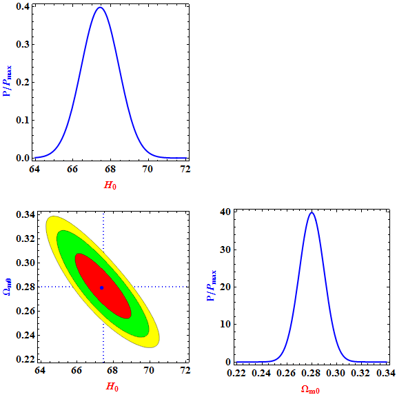
Figure 1: One-dimensional marginalized distributions and two dimensional contours at 1$\sigma$, 2$\sigma$ and 3$\sigma$ confidence regions in $H_{0}-\Omega_{m0}$ plane by bounding our model with 46 OHD points. The estimated values of $H_{0}=67.44~{}km~{}s^{-1}~{}Mpc^{-1}$ and $\Omega_{m0}=0.28$.

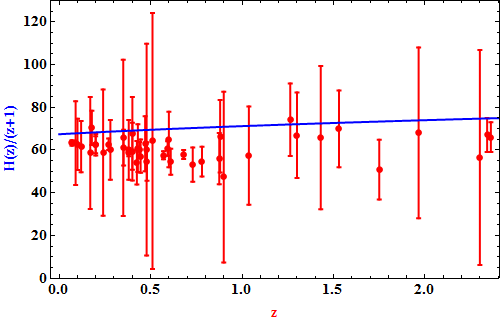
Figure 2: The Hubble rate versus red-shift error bar plot with 46 OHD points. The solid line represents our derived model.

Since, the present universe is filled with dust or dark matter which pressure is null $(p=0)$. Therefore, solving equations (5) - (7), we obtain

$$\frac{\ddot{a}}{a}+2\frac{\dot{a}^{2}}{a^{2}}=(\omega+1)\frac{\ddot{\phi}}{\phi}+(3\omega+2)\frac{\dot{a}\dot{\phi}}{a\phi}$$ (15)

The general solution of equation (18) is given by

$$\phi=\phi_{0}\left(\frac{a}{a_{0}}\right)^{\frac{1}{\omega+1}}$$ (16)

where $\phi_{0}$ and $a_{0}$ are constants.

Thus, the density parameters are read as

$$\Omega_{m}=\frac{8\pi\rho_{m}}{3c^{2}H^{2}\phi},~{}~{}\Omega_{\beta}=\frac{\beta^{2}}{4H^{2}}$$ (17)

where $\rho_{m}=\left(\rho_{m}\right)_{0}a^{-3}$ and $\Omega_{m}$ and $\Omega_{\beta}$ represent the dimensionless density parameters for matter and $\beta$- energy respectively.
Using equation (23) in equation (6), we obtain

$$\Omega_{m}+\Omega_{\beta}=1+\frac{5\omega+6}{6(\omega+1)^{2}}$$ (18)

The scale factor in term of red-shift is given by

$$a=\frac{a_{0}}{1+z},$$ (19)

Using equations (16), (23), (18) and (19) in equation (5), we obtain the expression for Hubble’s function in terms of red-shift as

$$H(z)=\frac{H_{0}}{\sqrt{1+\frac{5\omega+6}{6(\omega+1)^{2}}}}\left[1+\Omega_{m0}(1+z)^{\frac{3\omega+4}{\omega+1}}+\frac{5\omega+6}{6(\omega+1)^{2}}-\Omega_{m0}\right]^{\frac{1}{2}}$$ (20)

where $H_{0}$ and $\Omega_{m0}$ denote the present values of Hubble constant and matter energy density parameter respectively. In Table 1, H(z) is in unit of $km~{}s^{-1}~{}Mpc^{-1}$.

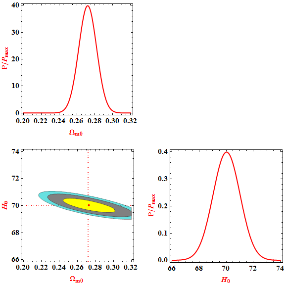
Figure 3: One-dimensional marginalized distributions and two dimensional contours at 1$\sigma$, 2$\sigma$ and 3$\sigma$ confidence regions in $\Omega_{m0}-H_{0}$ plane by bounding our model with SN Ia data points. The estimated values of $H_{0}=70.02~{}km~{}s^{-1}~{}Mpc^{-1}$ and $\Omega_{m0}=0.272$.

Table 1: Hubble parameter H(z) with redshift and errors $\sigma_{i}$.

S.N.	z	H(z)	$\sigma_{i}$	References
1	0	67.77	1.30	Macaulay/2018
2	0.07	69	19.6	Zhang/2014
3	0.09	69	12	Simon/2005
4	0.01	69	12	Stern/2010
5	0.12	68.6	26.2	Zhang/2014
6	0.17	83	8	Stern/2010
7	0.179	75	4	Moresco/2012
8	0.1993	75	5	Moresco/2012
9	0.2	72.9	29.6	Zhang/2014
10	0.24	79.7	2.7	Gazta/2009
11	0.27	77	14	Stern/2010
12	0.28	88.8	36.6	Zhang/2014
13	0.35	82.7	8.4	Chuang/2013
14	0.352	83	14	Moresco/2012
15	0.38	81.5	1.9	Alam/2016
16	0.3802	83	13.5	Moresco/2016
17	0.4	95	17	Simon/2005
18	0.4004	77	10.2	Moresco/2016
19	0.4247	87.1	11.2	Moresco/2016
20	0.43	86.5	3.7	Gazta/2009
21	0.44	82.6	7.8	Blake/2012
22	0.44497	92.8	12.9	Moresco/2016
23	0.47	89	49.6	Ratsimbazafy/2017
24	0.4783	80.9	9	Moresco/2016
25	0.48	97	60	Stern/2010
26	0.51	90.4	1.9	Alam/2016
27	0.57	96.8	3.4	Anderson/2014
28	0.593	104	13	Moresco/2012
29	0.6	87.9	6.1	Blake/2012
30	0.61	97.3	2.1	Alam/2016
31	0.68	92	8	Moresco/2012
32	0.73	97.3	7	Blake/2012
33	0.781	105	12	Moresco/2012
34	0.875	125	17	Moresco/2012
35	0.88	90	40	Stern/2010
36	0.9	117	23	Stern/2010
37	1.037	154	20	Moresco/2012
38	1.3	168	17	Stern/2010
39	1.363	160	33.6	Moresco/2015
40	1.43	177	18	Stern/2010
41	1.53	140	14	Stern/2010
42	1.75	202	40	Stern/2010
43	1.965	186.5	50.4	Moresco/2015
44	2.3	224	8	Busca/2013
45	2.34	222	7	Delubac/2015
46	2.36	226	8	Ribera/2014

• Observational Hubble Data (OHD): We adopt $46$ Observational Hubble Data (OHD) points over the redshift range of $0\leq z\leq 2.36$ (see table 1), obtained from cosmic chronometric (CC) technique. Since CC technique is based on the “galaxy differential age”method therefore OHD data obtained from CC technique is model-independent and not correlated.
  

• SN Ia Data: We use SN Ia data which includes 9 high $z$ and 27 low $z$, Gold Sample and New Gold Sample Vishwakarma/2018 and references therein.
  

For statistical analysis, we define $\chi^{2}$ as following:

$$\chi^{2}_{OHD}=\sum_{i=1}^{46}\left[\frac{H_{th}(z_{i})-H_{obs}(z_{i})}{\sigma_{i}}\right]^{2}$$ (21)

where $H_{obs}(z_{i})$ is the observed value of Hubble parameter with standard deviation $\sigma_{i}$ and $H_{th}(z_{i})$ is the theoretical value obtained from bounding equation (21) with 46 OHD points. The estimated values of $H_{0}=67.44~{}km~{}s^{-1}~{}Mpc^{-1}$ and $\Omega_{m0}=0.28$ with $\chi^{2}_{min}=26.36$.

Similarly for SN Ia data, we have estimated the model parameters $H_{0}$ and $\Omega_{m0}$ as $H_{0}=70.02~{}km~{}s^{-1}~{}Mpc^{-1}$ and $\Omega_{m0}=0.272$ with $\chi^{2}_{min}=562.22$. The numerical result is summarized in Table II. Figures 1 and 3 depict one-dimensional marginalized distributions and two dimensional contours at 1$\sigma$, 2$\sigma$ and 3$\sigma$ confidence regions by bounding our model with OHD and SN Ia data points respectively. The best fit curve for Hubble rate is exhibited in Figure 2.

Table 2: Summary of the numerical result.

Model parameters	OHD	SN Ia
$\Omega_{m0}$	$0.28$	$0.272$
$H_{0}$	$67.44$	$70.02$

IV Cosmological parameters of the model

IV.1 Deceleration parameter

The deceleration parameter of derived model in terms of red-shift is read as

$$q=-1+\frac{(1+z)H^{\prime}(z)}{H(z)}$$ (22)

where $H^{\prime}(z)$ is the first order derivative of H(z) with respect to z.

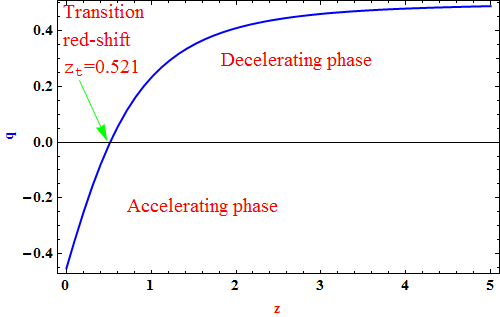
Figure 4: The variation of $q$ versus $z$ for $\Omega_{m0}=0.28$, $H_{0}=67.44~{}km~{}s^{-1}~{}Mpc^{-1}$ and $\omega=40000$.

Solving equations (20) and (22), we get

$$q=-1+\frac{(3\omega+4)\Omega_{m0}(z+1)^{\frac{3\omega+4}{\omega+1}}}{2(\omega+1)\left(-\Omega_{m0}+\Omega_{m0}(z+1)^{\frac{3\omega+4}{\omega+1}}+\frac{5\omega+6}{6(\omega+1)^{2}}+1\right)}$$ (23)

The graphical behaviour of deceleration parameter is depicted in Figure 4. From equation (23), one can obtain the present value of deceleration parameter as $q_{0}=-0.58$ by putting $z=0$, $\Omega_{m0}=0.28$ and $\omega=40000$. This value of $q_{0}$ is in pretty agreement with recent observations.

Figure 4 shows the signature flipping behavior of deceleration parameter with decreasing value of redshift i.e. at beginning $q$ was evolving with positive sign which indicates that early universe was in decelerating phase and it turns into accelerating mode at $z_{t}=0.521$. This transitioning evolution of $q$ from positive to negative value leads the concept of hybrid universe. In recent past, various cosmological models with hybrid expansion law have been investigated in different physical contexts Yadav/2019 ; Akarsu/2014 ; Yadav/2019b ; Yadav/2012 ; Pradhan/2011 ; Mishra/2018 ; Ray/2019 ; Yadav/2015 ; Yadav/2016 .

IV.2 Age of the universe

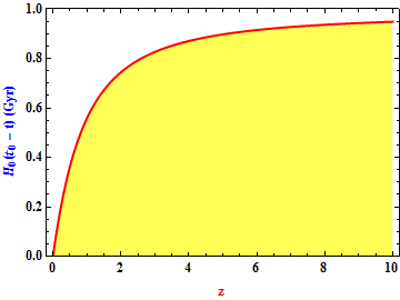
Figure 5: The plot of $H_{0}(t_{0}-t)$ versus $z$ for $\Omega_{m0}=0.28$, $H_{0}=67.44~{}km~{}s^{-1}~{}Mpc^{-1}\sim 0.0688\;Gyrs$ and $\omega=40000$. Here, we observe that for $z=0$, $H_{0}(t_{0}-t)$ becomes null which turns into imply that at present $t=t_{0}$.

The age of scalar field Brans-Dike universe is obtained as

$$H(z)=-\frac{1}{1+z}\frac{dz}{dt}\;\;\Rightarrow\;\;dt=-\frac{dz}{(1+z)H(z)}$$ (24)

Hence,

$$\int_{t_{0}}^{t}dt=-\int_{z}^{0}\frac{dz}{(1+z)\frac{H_{0}}{\sqrt{1+\frac{5\omega+6}{6(\omega+1)^{2}}}}\left[1+\Omega_{m0}(1+z)^{\frac{3\omega+4}{\omega+1}}+\frac{5\omega+6}{6(\omega+1)^{2}}-\Omega_{m0}\right]^{\frac{1}{2}}}$$ (25)

Here, $t_{0}$ is the present age of the universe and it is obtained as

$$t_{0}=\lim_{x\rightarrow\infty}{\int_{0}^{z}\frac{dz}{(1+z)\frac{H_{0}}{\sqrt{1+\frac{5\omega+6}{6(\omega+1)^{2}}}}\left[1+\Omega_{m0}(1+z)^{\frac{3\omega+4}{\omega+1}}+\frac{5\omega+6}{6(\omega+1)^{2}}-\Omega_{m0}\right]^{\frac{1}{2}}}}$$ (26)

Integrating equation (26), we obtain

$$H_{0}t_{0}=0.983019$$ (27)

Thus the present age of the universe is computed as $t_{0}=0.983019~{}H_{0}^{-1}=14.288\;Gyrs$. It is important to note that the present age of the universe in derived model nicely match with its empirical value, predicted by recent WMAP observations Hinshaw/2013 and Plank collaborations Ade/2014 . Therefore, the model under consideration have pretty consistency with recent astrophysical observations Ade/2014 ; Hinshaw/2013 .

IV.3 Jerk parameter

The jerk parameter (j) Mukherjee/2019 , in terms of red-shift and Hubble function is read as

$$1-(1+z)\frac{[H(z)^{2}]^{\prime}}{H(z)^{2}}+\frac{1}{2}(1+z)^{2}\frac{[H(z)^{2}]^{\prime\prime}}{H(z)^{2}}$$ (28)

Equations (20) and (28) lead to

$$j=1-\frac{3(\omega+1)(3\omega+4)\Omega_{m0}(z+1)^{\frac{3\omega+4}{\omega+1}}}{6(\omega+1)^{2}\Omega_{m0}\left((z+1)^{\frac{3\omega+4}{\omega+1}}-1\right)+6\omega^{2}+17\omega+12}+$$

$$\frac{9(3\omega+4)^{2}\Omega_{m0}^{2}(z+1)^{\frac{4\omega+6}{\omega+1}}\left(3(\omega+1)^{2}\Omega_{m0}\left(2\left((z+1)^{\frac{3\omega+4}{\omega+1}}-3\right)+\omega\left((z+1)^{\frac{3\omega+4}{\omega+1}}-4\right)\right)+\xi\right)^{2}}{2\left(6(\omega+1)^{2}\Omega_{m0}\left((z+1)^{\frac{3\omega+4}{\omega+1}}-1\right)+6\omega^{2}+17\omega+12\right)^{4}}$$ (29)

where $\xi=(2\omega+3)^{2}(3\omega+4)$.

The explicit expression of jerk parameter is given in equation (29) and its behavior is graphed in Figure 5. We observe that for high red-shift values, the jerk parameter have its low values and it increases as $z$ decreases. The present value of jerk parameter is computed as $j_{0}=0.8002$. Therefore, the derived model represents a model of the universe other than $\Lambda$CDM universe. Note that $H$, $q$ and $j$ are the important parameters of cosmographic series. The usefulness of these parameters in discriminating the various dark energy models are given in Refs. CAPOZZIELLO/2019 ; Dunsby/2016 .

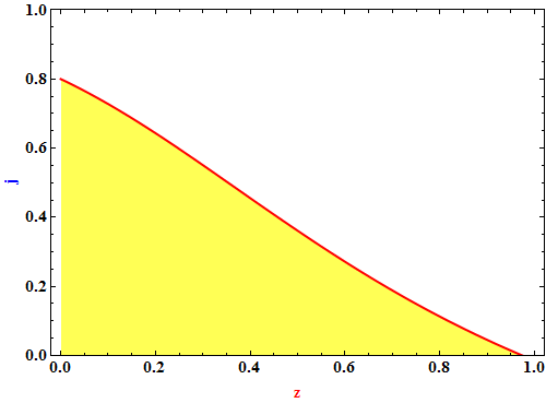
Figure 6: The plot of $j$ versus $z$ for $\Omega_{m0}=0.28$ and $\omega=40000$.

V Concluding remarks

In this paper, we have investigated a scalar field Brans-Dicke cosmological model in Lyra’s manifold and also checked its validity by performing well known $\chi^{2}$ test for free parameters of the model with recent observational H(z) and SN Ia data. The derived model successfully passes this test on the scale of statistical analysis and represents the best fit curve for Hubble rate (see Fig. 2). The present values of deceleration parameter and age of the universe are calculated in section IV. We observe that the model under consideration have pretty consistency with recent Plank collaboration results and WMAP observations which in turn implies that the derived model is physically viable. Figure 4 exhibits that the universe in derived model evolves with negative deceleration parameter i.e. the present universe expands with acceleration due to accumulation of matter in scalar field. So, the proposed model describes features of the universe from early decelerating phase to current accelerating phase without inclusion of any exotic type matter or energy. The natural behavior of jerk parameter of scalar field Brans-Dicke universe in Lyra’s manifold is shown in Figure 6. It is worthwhile to note that the displacement vector $\beta$ does not behave like $\Lambda$ - particularly in contributing the late time acceleration of the universe however the scalar field $\phi$ dominates the current universe. Finally in spite of very good possibility of co-existence of Brans-Dicke gravity and Lyra’s geometry to provide a theoretical foundation for relativistic gravitation, astrophysics and cosmology, the experimental point is yet to be considered. But still the theory needs a fair trial.

Acknowledgments: The authors are grateful to the reviewer for illuminating suggestions that have significantly improved our work in terms of research quality and presentation. The authors are grateful to Y. Heydarzade for fruitful comments on the paper.

References

- (1) L. Iorio, Editorial for the special issue 100 years of chronogeometrodynamics: The status of the Einstein’s theory of gravitation in its centennial year, Universe 1 (2015) 38-81.
- (2) I. Debono, G. F. Smoot, General relativity and cosmology: Unsolved questions and future directions, Universe 2 (2016) 23.
- (3) R. G. Vishwakarma, Einstein and beyond: A critical perspective on general relativity, Universe 2 (2016) 16.
- (4) J. B. Jimenez, L. Heisenberg, T. S. Koivisto, The Geometrical trinity of gravity, Universe 5 173 (2019)
- (5) S. Kumar, Some FRW models of accelerating universe with dark energy, Astrophys. Space Sc. 332 (2011) 449-454.
- (6) E. J. Copeland, M. Sami, S. Tsujikawa, Dynamics of dark energy, Int. J. Mod. Phys. D 15 (2006) 1753-1935.
- (7) A. K. Yadav, F. Rahaman, S. Ray, Dark energy models with variable equation of state parameter, Int. J. Theor. Phys. 50 (2011) 871.
- (8) A. K. Yadav, Some anisotropic dark energy models in Bianchi type-V space-time, Astrophys. Space Sc. 335 (2011) 565-575.
- (9) S. Kumar, A. K. Yadav, Some Bianchi type-V models of Accelerating universe with dark energy, Mod. Phys. Lett. A 26 (2011) 647-659.
- (10) A. K. Yadav, L. Yadav, Bianchi type III anisotropic dark energy models with constant deceleration parameter, Int. J. Theor. Phys. 50 (2011) 218-227.
- (11) A. K. Yadav et al, Magnetized dark energy and the late time acceleration, Euro. Phys. J. Plus 127 (2012) 127.
- (12) T. Clifton, P. G. Ferreira, A. Padilla, C. Skordis, Modified gravity and cosmology, Physics Reports 513 (2012) 1-189.
- (13) S. Capozziello, T. Harko, T. S. Koivisto, F. S. N. Lobo, G. J. Olmo, Hybrid metric-Palatini gravity, Universe 1 (2015) 199-238.
- (14) I. de Martino, M. De Laurentis, S. Capozziello, Constraining gravity by the large scale structure, Universe 1 (2015) 123-157
- (15) G. Lyra, Ubereine Modifikation der Riemannschen Geometrie, Math. Z. 54 (1951) 52.
- (16) C. Brans, R. H. Dicke, Mach’s principle and a relativistic theory of gravitation, Phys. Rev. D 124 (1961) 925.
- (17) W. D. Halford, Scalar-Tensor theory of gravitation in a Lyra manifold J. Math. Phys. 13 (1972) 1399.
- (18) F. Darabi, Y. Heydarzade, F. Hajkarim, Stability of Einstein static universe over Lyra geometry, Can. J. Phys. 93 2015 1566.
- (19) G. F. R. Ellis, R. Maartens, The emergent universe: inflationary cosmology with no singularity, Class. Quant. Grav. 21 2004 223.
- (20) G. P. Singh, K. Desikan, A new class of cosmological models in Lyra geometry, Pramana 49 (1997) 205-212.
- (21) A. Pradhan, L. Yadav, A. K. Yadav, Isotropic homogeneous universe with a bulk viscous fluid in Lyra geometry Astrophys. Space Sc. 299 (2005) 31
- (22) A. K. Yadav, Lyra’s cosmology of inhomogeneous universe with electromagnetic field, Fizika B 19 (2009) 53.
- (23) T. Singh, G. Singh, Bianchi type III and Kantowski-Sachs cosmological models in Lyra geometry, Int. J. Theor. Phys. 31 (1992) 1433.
- (24) T. Singh, G. Singh, Lyra’s geometry and cosmology, Fortschritte der Physik 41 (1993) 737-764.
- (25) A. K. Yadav, A. Haque, Lyra’s cosmology of massive strings in anisotropic Bianchi-II space-time, Int. J. Theor. Phys. 50 (2011) 2850.
- (26) F. Rahaman, B. C. Bhui, G. Bag, Can Lyra geometry explain the singularity free as well as accelerating Universe Astrophys. Space Sc. 295 (2005) 507.
- (27) V. K. Yadav, L. Yadav, A. K. Yadav, New exact solution of Bianchi type V cosmological model in Lyra’s geometry Rom. J. Phys. 55 (2010) 862.
- (28) A. K. Yadav, V. K. Bhardwaj, Lyra’s cosmology of hybrid universe in Bianchi-V space-time Res. Astron. Astrophys. 18 (2018) 64.
- (29) A. K. Yadav, Comment on Brans-Dicke scalar field cosmological model in Lyra’s geometry, Phys. Rev. D 102 (2020) 108301.
- (30) P. Mukherjee, S. Chakrabarti, Exact solutions and accelerating universe in modified Brans-Dicke theories Euro. Phys. J. C. 79 (2019) 681.
- (31) D. C. Maurya, R. Zia, Brans-Dicke scalar field cosmological model in Lyra’s geometry, arXiv: 1907.07135[gr-qc].
- (32) G. K. Goswami, Cosmological parameters for spatially flat dust filled universe in Brans-Dicke theory,arXiv: 1710.07281 [gr-qc].
- (33) A. K. Yadav, H. Amirhashchi, Constraining an exact Brans-Dicke gravity theory with recent observations, arXiv: 1908.04735 [gr-gc].
- (34) S. Sen, A. A. Sen, Late time acceleration in Brans-Dicke cosmology, Phys. Rev. D 63 (2001) 124006.
- (35) O. Akarsu, N. Katirci, N. Ozedemir, J. A. Vazquez, Anisotropic massive Brans-Dicke gravity extension of the standard CDM model, arXiv: 1903.06679 [gr-qc].
- (36) B. Bertotti et al, A test of general relativity using radio links with the Cassini spacecraft, Nature 425 (2003) 374.
- (37) A. D. Felice et al, Relaxing nucleosynthesis constraints on Brans-Dicke theories, Phys. Rev. D 74 (2006) 103005.
- (38) A. Jawed et al, Modified holographic Ricci dark energy in chameleon Brans–Dicke cosmology and its thermodynamic consequence, Comm. Theor. Phys. 63 (2015) 453.
- (39) K. D. Naidu, D. R. K. Reddy, Y. Aditya, Dynamics of axially symmetric anisotropic modified holographic Ricci dark energy model in Brans-Dicke theory of gravitation, Eur. Phys. J. Plus 133 (2018) 303.
- (40) M. Kiran et al, Minimally interacting holographic Dark energy model in Brans-Dicke theory, Astrophys. Space Sc. 356 (2015) 407.
- (41) G. Ramesh, S. Umadevi, LRS Bianchi type-II minimally interacting holographic dark energy model in Saez-Ballester theory of gravitation, Astrophys. Space Sc. 361 (2016) 50.
- (42) Z. Yousaf, On the role of f(G,T) terms in structure scalars, Eur. Phys. J. Plus 134 (2019) 245.
- (43) Z. Yousaf, Hydrodynamic properties of dissipative fluids associated with tilted observers, Mod. Phys. Lett. A 34 (2019) 1950333.
- (44) E. Macaulay et al, First cosmological results using Type Ia Supernovae from the dark energy survey: measurement of the Hubble constant, arXiv: 1811.02376.
- (45) C. Zhang et al, Four new observational H(z) data from luminous red galaxies in the Sloan Digital Sky Survey data release seven, Res. Astron. Astrophys 14 (2014) 1221.
- (46) J. Simon, L. Verde, R. Jimenez, Constraints on the redshift dependence of the dark energy potential Phys. Rev. D 71 (2005) 123001.
- (47) D. Stern et al, Cosmic chronometers: constraining the equation of state of dark energy I: H(z) measurements JCAP 1002 (2010) 008.
- (48) M. Moresco et al, Improved constraints on the expansion rate of the Universe up to z 1.1 from the spectroscopic evolution of cosmic chronometers, JCAP 08 (2012) 006.
- (49) E. Gazta Naga et al, Clustering of luminous red galaxies – IV. Baryon acoustic peak in the line-of-sight direction and a direct measurement of H(z) MNRAS 399 (2009) 1663.
- (50) D. H. Chuang, Y. Wang, Modelling the anisotropic two-point galaxy correlation function on small scales and single-probe measurements of H(z), and f(z) from the Sloan Digital Sky Survey DR7 luminous red galaxies, MNRAS 435 (2013) 255.
- (51) S. Alam et al, The clustering of galaxies in the completed SDSS-III Baryon Oscillation Spectroscopic Survey: cosmological analysis of the DR12 galaxy sample, MNRAS 470 (2016) 2617.
- (52) M. Moresco et al, A measurement of the Hubble parameter at : direct evidence of the epoch of cosmic re-acceleration, JCAP 05 (2016) 014.
- (53) C. Blake et al, The WiggleZ Dark Energy Survey: joint measurements of the expansion and growth history at , MNRAS 425 (2012) 405.
- (54) A. L. Ratsimbazafy et al, The WiggleZ dark Energy Survey: joint measurements of the expansion and growth history at , MNRAS 467 (2017) 3239.
- (55) L. Anderson et al, The clustering of galaxies in the SDSS-III Baryon Oscillation Spectroscopic Survey: baryon acoustic oscillations in the Data Releases 10 and 11 Galaxy samples, MNRAS 441 (2014) 24.
- (56) M. Moresco, Raising the bar: new constraints on the Hubble parameter with cosmic chronometers at , MNRAS 450 (2015) L16.
- (57) N. G. Busca et al, Baryon acoustic oscillations in the forest of BOSS quasars, Astron & Astrophys. 552 (2013) A96.
- (58) T. Delubac et al, Which fundamental constants for cosmic microwave background and baryon-acoustic oscillation?, Astron & Astrophys 584 (2015) A69.
- (59) A. Font-Ribera et al, Quasar-Lyman forest cross-correlation from BOSS DR11: Baryon Acoustic Oscillations, JCAP 1405 (2014) 027.
- (60) R. G. Vishwakarma, J. V. Narlikar, Is it no longer necessary to test cosmologies with type SN Ia supernovae? Universe 4 (2018) 73.
- (61) A. K. Yadav, Transitioning scenario of Bianchi-I universe within formalism, Braz. J. Phys. 49 (2019) 262.
- (62) O. Akarsu, S. Kumar, R. Ayrzakulov, M. Sami and L. Xu, Cosmology with hybrid expansion law: scalar field reconstruction of cosmic history and observational constraints J. Cosmol. Astropart. Phys. 1 (2014) 022.
- (63) A. K. Yadav, P. K. Sahoo, V. K. Bhardwaj, Bulk Viscous Bianchi-I Embedded Cosmological Model in Gravity, Mod. Phys. Lett. A 34 (2019) 1950145.
- (64) A. K. Yadav, Bianchi-V string cosmological model and late time acceleration, Res. Astron. Astrophys. 12 (2012) 1467.
- (65) A. Pradhan, H. Amirhashchi, Accelerating dark energy models in Bianchi type V space-time, Mod. Phys. Lett. A 26 (2011) 2261.
- (66) B. Mishra, S. K. Tripathy, S.Tarai, Cosmological models with a hybrid scale factor in an extended gravity theory, Mod. Phys. Lett. A 33 (2018) 1850052.
- (67) P. P. Ray, B. Mishra, S. K. Tripathy, Dynamics of anisotropic dark energy universe embedded in one-directional magnetized fluid Int. J. Mod. Phys. D 28 (2019) 1950093.
- (68) A. K. Yadav, P. K. Srivastava, L. Yadav, Hybrid expansion law for dark energy dominated universe in Gravity, Int. J. Theor. Phys. 54 (2015) 1671.
- (69) A. K. Yadav, A transitioning universe with anisotropic dark energy, Astrophys. Space Sc. 361 (2016) 276.
- (70) G. Hinshaw et al., Nine-year Wilkinson Microwave Anisotropy Probe (WMAP) observations: cosmological parameter results, Astrophys. J. Supp. Sr. 208 (2013) 19.
- (71) P. A. R. Ade et al., Planck 2013 results XVI cosmological parameters. Astron. Astrophys. 571 (2014) A16.
- (72) S. Capozziello, R. D’Agostino, O. Luongo, Extended gravity cosmography, Int. J. Mod. Phys. D 28 (2019) 1930016.
- (73) P. K. S. Dunsby and O. Luongo, On the theory and applications of modern cosmography, Int. J. Geom. Meth. Mod. Phys. 13 (2016) 1630002.