Influence of Wolf–Rayet stars on surrounding star-forming molecular clouds

Abstract

We investigate the influence of Wolf–Rayet (W–R) stars on their surrounding star-forming molecular clouds. We study five regions containing W–R stars in the inner Galactic plane ($l\sim$[14^∘–52^∘]), using multi-wavelength data from near-infrared to radio wavelengths. Analysis of ¹³CO line data reveals that these W–R stars have developed gas-deficient cavities in addition to molecular shells with expansion velocities of a few km s^-1. The pressure owing to stellar winds primarily drives these expanding shells and sweeps up the surrounding matter to distances of a few pc. The column densities of shells are enhanced by a minimum of 14% for one region to a maximum of 88% for another region with respect to the column densities within their central cavities. No active star formation — including molecular condensations, protostars, or ionized gas — is found inside the cavities, whereas such features are observed around the molecular shells. Although the expansion of ionized gas is considered an effective mechanism to trigger star formation, the dynamical ages of the H ii regions in our sample are generally not sufficiently long to do so efficiently. Overall, our results hint at the possible importance of negative W–R wind-driven feedback on the gas-deficient cavities, where star formation is quenched as a consequence. In addition, the presence of active star formation around the molecular shells indicates that W–R stars may also assist in accumulating molecular gas, and that they could initiate star formation around those shells.

1. Introduction

Wolf–Rayet (W–R) stars are post-main-sequence stars that have descended from their early O-type progenitors ($m_{\ast}\gtrsim 20M_{\odot}$). W–R stars are characterized by enormous mass-loss rates, $\sim 10^{-5}M_{\odot}$ yr^-1, with a wind velocity of 1000–5000 km s^-1 (Crowther, 2007). Given such strong energetics, W–R stars can significantly affect their natal environments despite their short life span ($\sim$5 Myr; Lamers & Cassinelli, 1999). In fact, the energetics associated with less massive OB stars ($m_{\ast}\gtrsim 8M_{\odot}$ but $m_{\ast}<20M_{\odot}$), such as stellar winds and ultraviolet (UV) radiation, are observationally found to influence and shape their surrounding interstellar medium (ISM; Motte et al., 2018). Their strong energetic impact may either trigger the formation of the next generation of stars or disperse the surrounding molecular gas into the ISM, and thus halt further star formation (Deharveng et al., 2010). Two primary theories are thought to explain the triggered star formation mechanism. One is the ‘collect and collapse’ scenario, where molecular gas is collected between the ionization and shock fronts developed by the massive star and eventually collapses to form stars once a critical density is reached (Elmegreen & Lada, 1977; Elmegreen, 1998). The alternative theory is ‘radiation-driven implosion’, where UV photons from massive stars initiate the formation of the next generation of stars in the surrounding, pre-existing cores (Reipurth, 1983; Bertoldi, 1989; Lefloch & Lazareff, 1994). Observational evidence of next generation star formation triggered by massive stars is found in several Galactic star-forming regions (see e.g., Dewangan et al., 2016; Zavagno et al., 2010a, b; Pomarès et al., 2009, and references therein). For example, evidence of the ‘collect and collapse’ process is seen around several H ii regions where second-generation stars were found in the periphery of the ionized gas (Zavagno et al., 2007; Deharveng et al., 2008). The ‘radiation-driven implosion’ process is also notably observed in several bright-rimmed clouds, as evidenced by e.g., aligned and sequential star formation with respect to the energetic source (see e.g. Ogura et al., 2007; Urquhart et al., 2007; Morgan et al., 2010; Panwar et al., 2014, and references therein).

The influence of W–R stars on their parent clouds might be significantly different from what is typically seen around less massive OB stars or H ii regions. The effect of a W–R star on its parent molecular cloud could either be positive or negative in the context of next generation star formation triggers. Owing to its energetic stellar wind, a W–R star may create a surrounding cavity and develop wind-blown expanding shells of parsecs to tens of parsecs scales with typical expansion velocities of a few km s^-1 (Marston, 1996). Triggering mechanisms may occur at the boundary of the expanding molecular shell (Whitworth et al., 1994). However, based on hydrodynamic simulations of turbulent giant molecular clouds, Dale et al. (2013) reported that the efficiency of wind-driven triggering to initiate star formation is low compared with that of the ionized gas. The presence of a W–R star instead may destroy favorable conditions for further star formation by driving away the surrounding molecular gas into the ISM (Dale et al., 2013; Sokal et al., 2016). Sokal et al. (2016) studied several massive star clusters associated with W–R stars and suggested that the presence of a W–R star may accelerate cluster emergence. On the other hand, a positive impact of W–R stars on their parent clouds, leading to further star formation, was also found in a few Galactic regions (see Liu et al., 2012; Dewangan et al., 2016, and references therein).

Observational studies of star-forming regions associated with W–R stars are limited mainly because of their rarity and also since a large fraction of W–R stars are still unknown in the Milky Way (Crowther, 2007). Recent systematic surveys aimed at identifying Galactic W–R stars (e.g. Shara et al., 2012; Kanarek et al., 2015) have increased their number by a factor of two with respect to the previous decade. This study aims to explore a few potential star-forming regions that could be associated with W–R stars and, subsequently, to examine whether the presence of W–R stars has any impact on the surrounding molecular gas. We perform an analysis of multi-wavelength data from near-infrared (NIR) to radio wavelengths to investigate the star formation activity in the clouds surrounding W–R stars. Note that massive star-forming regions are often associated with H ii regions, which may also have a large impact on triggered star formation (Deharveng et al., 2010).

Since the advent of the Spitzer Space Telescope, thousands of parsec-scale mid-infrared (MIR) Galactic bubbles have been identified in Spitzer-IRAC 8 $\mu m$ images (Churchwell et al., 2006, 2007; Simpson et al., 2012). Deharveng et al. (2010) reported active star formation in many of those MIR Galactic bubbles. Thus, MIR bubbles could be suitable regions for our study, provided they are associated with W–R stars. This study is organized as follows. The details of the selected regions, their associated MIR Galactic bubbles, and spatially overlapping W–R stars are presented in Section 2 (see also Table 1). Section 3 describes the details of the multi-wavelength data sets used in the analysis. In Section 4, we explore the possibility that these W–R stars may be associated with individual molecular clouds. Then, in Section 5 we perform an analysis to examine the dynamics of molecular gas using molecular-line data and ongoing star formation activity, if any, toward these regions. A detailed discussion of the possible influence of W–R stars on their surrounding molecular clouds is offered in Section 6. Finally, we provide our conclusions in Section 7.

2. Selected regions

We cross-matched the available catalogs of W–R stars (van der Hucht, 2001, 2006; Hadfield et al., 2007; Shara et al., 2012; Kanarek et al., 2015) with the Spitzer–Galactic Legacy Infrared Mid-Plane Survey Extraordinaire (GLIMPSE; Benjamin et al., 2003) MIR Galactic bubble catalogs (Churchwell et al., 2006, 2007; Simpson et al., 2012), employing a search radius of twice the effective bubble radius. This particular radius was chosen for our cross-matching, assuming that a W–R star located outside the bubble periphery but at a separation of twice the radius of the MIR bubble might have a strong impact on the gas around the bubble — even though it might not be the primary driving source for the bubble to form. The primary aim of this study is not to search for the effect of W–R stars on MIR bubbles but to examine their influence on surrounding star-forming parental clouds. The role of MIR bubbles here is only to help us in identifying regions exhibiting active star formation. It is important to note that Deharveng et al. (2010) found that at least 86% of the bubbles are associated with ionized gas. Thus, most of these bubbles can be considered active massive star-forming regions.

We found spatial matches for about 30 regions. We further limited the identified regions to only those for which molecular-line (¹³CO) data are available with a good velocity resolution (i.e. data from the Galactic Ring Survey, GRS; $l\sim$[14^∘–55^∘]; see Section 3.4). W–R stars with poorly constrained spectral types have also been excluded from this study. Finally, our combined selection criteria yield six potential regions for further study. However, one of these (MIR bubble N46) has already been studied extensively by Dewangan et al. (2016). Thus, in this paper we explore five Galactic regions to examine the influence of W–R stars on their parent molecular clouds. Additional analysis of the well-studied bubble N46 (Dewangan et al., 2016) is performed primarily to serve as a reference. An overview of our five selected regions and the bubble N46 (region G27 in this paper) is presented below (see Table 1 for a summary).

2.1. G15.010–0.570

The region G15.010–0.570 (hereafter G15) is located at Galactic coordinates $l$=15^∘.010, $b$=$-$0^∘.570. Figure 1 shows a three-color composite image of a large area around the region (red: Herschel 70 $\mu$m; green: Spitzer-IRAC 8 $\mu$m; blue: Spitzer-IRAC 3.6 $\mu$m). The Jansky Very Large Array (VLA) Galactic Plane survey (VGPS) radio continuum contours at 1.4 GHz are also superimposed. Contours of the integrated ¹³CO map of the host molecular cloud (the identification procedure of host molecular cloud is discussed in Section 4; see also Table 1) are also overlaid. The region hosts two MIR bubbles, N15 and MWP1G015131–005253, and a W–R star, 2MASS J18192219–1603123, located at the edge of the bubble MWP1G015131–005253. This W–R star was first identified and classified as a WN7o star by Hadfield et al. (2007). The W–R star has a Gaia parallax of 0.42$\pm$0.14 milli-arcsec (Gaia Collaboration et al., 2018), which corresponds to a distance of 2.3${}^{+1.3}_{-0.6}$ kpc (estimated using a Bayesian approach by Bailer-Jones et al., 2018).

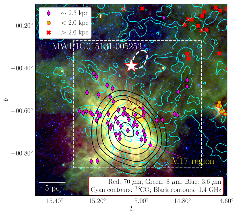
Figure 1.— Three-color composite image (red: 70 $\mu$m; green: 8 $\mu$m; blue: 3.6 $\mu$m) around the G15 region. The position of the W–R star, 2MASS J18192219–1603123, is marked by a white star. Two MIR bubbles, N15 and MWP1G015131–005253, are marked by brown and white dashed ellipses, respectively. The 1.4 GHz VGPS contours are shown in black at levels of 100, 150, 200, 300, 400, and 500 mJy beam^-1. Cyan contours represent the integrated ¹³CO gas of the host molecular cloud toward the region. A scale bar corresponding to a projected separation of 5 pc is also shown in the bottom left-hand corner. The dust clumps identified by Urquhart et al. (2018) are marked by diamonds, hexagons, and crosses, depending on their distances (see legend). The area shown in the white dashed box is the region selected for further analysis.

The famous Omega Nebula (Messier 17 or M17; distance $\sim$2.0 kpc; Wu et al., 2014) is spatially located adjacent to the W–R star. M17 is regarded one of the most active massive Galactic star-forming regions, with a star-formation rate $\geq$ $0.004~{}M_{\odot}$ yr^-1(see Povich et al., 2016, and references therein). Chibueze et al. (2016) identified hundreds of H₂O maser sources in the M17 region spanning a local standard of rest velocity ($v_{\mathrm{LSR}}$) range of 14.0–22.0 km s^-1. They also reported a distance to the region of 2.04${}^{+0.16}_{-0.17}$ kpc, based on trigonometric parallaxes of the H₂O masers. This similarity in distances and the spatial proximity of the W–R star to M17 imply that they could be part of the same molecular cloud. The G15 region also hosts a large-scale gaseous filament known as F18 at a distance of 2.0 kpc (see Wang et al., 2016).

Recently, Urquhart et al. (2018) reported distances for thousands of 870 $\mu$m dust clumps toward the inner Galactic plane. They resolved the distance ambiguities of these clumps using measurements from Hi line observations, maser parallaxes, and spectroscopic observations. Several dust clumps were identified toward this region, primarily located at distances of 2.0–2.6 kpc in the $v_{\mathrm{LSR}}$ range of 16–30 km s^-1. Finally, considering the distances and the distribution of the dust clumps, we selected a 36${}^{\prime}\times$36^′ area centered at $l$=15^∘.010, $b$=$-$0^∘.570 for further analysis (see Figure 1).

2.2. G24.750+0.100

A three-color composite image (red: Herschel 70 $\mu$m; green: Spitzer-IRAC 8 $\mu$m; blue: Spitzer-IRAC 3.6 $\mu$m) of a large area around the G24.750+0.100 region (hereafter G24) is shown in Figure 2. The distribution of ionized gas in the region is shown by the VGPS 1.4 GHz radio continuum contours. The distribution of ¹³CO gas of the host molecular cloud is also shown. The region includes two MIR bubbles, N35 and N36, and the W–R star 1477-55L. This W–R star was first identified by Shara et al. (2012), and classified as a WC9 star. Although, Shara et al. (2012) reported a foreground extinction to the W–R star of $A_{K_{\mathrm{s}}}\sim 3.03$ mag, but no distance estimate was given by these authors. The region is also associated with a large gaseous filament, F27, located at a distance of 5.6 kpc (Wang et al., 2016). The presence of two molecular clumps, U24.50–0.04 and C24.48+0.21, toward the region are found at $v_{\mathrm{LSR}}$ of 110.3 and 117.5 km s^-1, respectively. The corresponding distances are 9.1 and 8.6 kpc (Anderson et al., 2012).

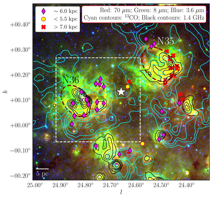
Figure 2.— Three-color composite image (red: 70 $\mu$m; green: 8 $\mu$m; blue: 3.6 $\mu$m) around the G24 region. The position of the W–R star, 1477–55L, is marked by a white star. Two MIR bubbles, N35 and N36, are marked by brown dashed ellipses. The 1.4 GHz VGPS contours are shown in black at levels of 40, 50, 65, 80, 100, 150, and 200 mJy beam^-1. In addition, cyan contours show the distribution of the ¹³CO gas of the host cloud. The remaining symbols are similar to those in Figure 1.

The ionized gas associated with these clumps is characterized by $v_{\mathrm{LSR}}$ of 108.1 and 115.7 km s^-1, respectively. The dust clumps toward this region (Urquhart et al., 2018) are located in two different velocity ranges. Clumps at a distance of $\sim$6 kpc have $v_{\mathrm{LSR}}$ in the range 98–114 km s^-1, whereas clumps located further than 7 kpc typically have $v_{\mathrm{LSR}}$ greater than 115 km s^-1. Accordingly, Figure 2 shows that the bubbles N35 and N36 may be associated with two different distances. The distance estimate to the W–R star, 1477–55L, of 5.7$\pm$0.5 kpc (see Section 4.1; see also Table 1) implies that it is likely associated with the cloud hosting the MIR bubble N36.

Recently, Dewangan et al. (2018) performed a detailed study of this region, primarily to reveal the formation of the N36 bubble. They found evidence of a collision between two nearby molecular clouds toward N36. Even so the primary goal and the area of this study are significantly different from those of Dewangan et al. (2018). Based on the distribution as well as the distances to the dust clumps, we selected a 20${}^{\prime}\times$20^′ area centered at $l$=24^∘.750, $b$=+0^∘.100 for further analysis.

2.3. G34.260+0.169

A three-color composite image of the G34.260+0.169 region (hereafter G34) is shown in Figure 3. This region hosts a WC8-type W–R star, 1553-15DF (Kanarek et al., 2015). Wang et al. (2016) reported the presence of a gaseous filament, F36, at a distance of 1.6 kpc projected toward this region. The G34 region also harbors an infrared dark cloud (IRDC), G34.43+0.24, which was explored to look for high-mass star-forming cores by Xu et al. (2016) and Sakai et al. (2018). Xu et al. (2016) found that the IRDC is located at a $v_{\mathrm{LSR}}$ range of 53–63 km s^-1 and suggested that it could be divided into three parts based on the prevailing evolutionary stages. The IRDC has multiple distance measurements, ranging from 1.56 kpc to 3.9 kpc (Faúndez et al., 2004; Rathborne et al., 2006; Simon et al., 2006; Kurayama et al., 2011; Foster et al., 2012). However, the distance of 1.56 kpc, measured using a H₂O maser parallax by Kurayama et al. (2011), is controversial since there was only a single background source for reference (Foster et al., 2012).

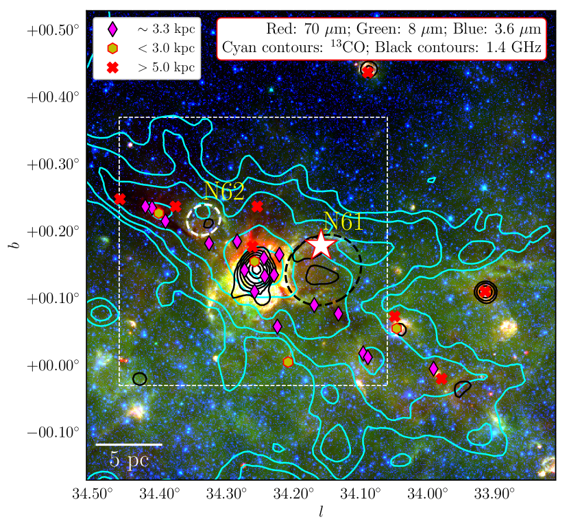
Figure 3.— Three-color composite image of the region around G34. The position of the W–R star, 1553–15DF, is marked by a white star. The region hosts two MIR bubbles, N61 and N62, which are marked by dashed black and white ellipses, respectively. The 1.4 GHz VGPS contours (in black) are shown at levels of 28, 42, 70, 120, 200, 400, and 600 mJy beam^-1, while cyan contours show the distribution of ¹³CO gas of the host cloud. The remaining symbols are similar to those in Figure 1.

The region also hosts two MIR bubbles, N61 and N62, and at least two molecular clumps (U34.26+0.15 and U34.40+0.23; Anderson et al., 2012) at a $v_{\mathrm{LSR}}$ of about 57 km s^-1. Clump U34.26+0.15 is located at a distance of 3.4$\pm$0.5 kpc (Anderson et al., 2012). Xu et al. (2016) suggested that the bubble N61 may be associated with the IRDC G34.43+0.24. However, the other bubble, N62, is located at the far kinematic distance ($d_{\mathrm{Far}}$) of 10.55 kpc, and has no physical association with the IRDC (Devine et al., 2018). Dust clumps near the W–R star are projected onto a filamentary structure (see Figure 3), and these clumps have distances of $\sim$3.3 kpc ($v_{\mathrm{LSR}}$ $\in 53$–59 km s^-1) which are similar to the distance to the W–R star (2.9$\pm$0.3 kpc; see Table 1 and Section 4.1). Based on the distribution of the dust clumps, we selected a 24${}^{\prime}\times$24^′ area centered at $l$=34^∘.260, $b$=+0^∘.169 for further analysis.

2.4. G35.598–0.032

The G35.598–0.032 region (hereafter G35) hosts a WC7 star, 1567-51L (Shara et al., 2012). It also harbors two MIR Galactic bubbles, N67 and N68. The W–R star is located toward the edge of N67 (see Figure 4). Zhang & Wang (2013) studied N68 and its environment using multi-wavelength data sets. They concluded that the expansion of the H ii region has affected the surrounding molecular gas for further star formation.

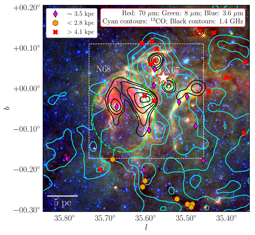
Figure 4.— Three-color composite image of the G35 region. The position of the W–R star, 1567–51L, is marked by a white star. This region also hosts two MIR bubbles, N67 and N68, which are marked by dashed green ellipses. The 1.4 GHz VGPS contours (in black) are overplotted at levels of 30, 35, 45, 60, and 80 mJy beam^-1. Distribution of the ¹³CO gas of the host cloud is also shown in cyan contours. The remaining symbols are similar to those in Figure 1.

Several cold clumps are found around this region (Anderson et al., 2012). They are located at a $v_{\mathrm{LSR}}$ range of 51–56 km s^-1. Dust clumps (Urquhart et al., 2018) spatially close to the W–R star in this region are found at distances of $\sim$3.5 kpc ($v_{\mathrm{LSR}}$ range of 46–64 km s^-1). Considering the distance to the W–R star (3.8$\pm$0.4 kpc; see Table 1) and the associated dust clumps, we have selected a 17${}^{\prime}\times$17^′ area centered at $l$=35^∘.598, $b$=$-$0^∘.032 for further analysis.

2.5. G51.840+0.410

The G51.840+0.410 region (hereafter G51) harbors a W–R star, 1697-38F, which is classified as WC9 (Kanarek et al., 2015) and hosts two MIR bubbles, N108 and N109 (see Figure 5). Bania et al. (2012) noted star formation toward the edge of N109, and identified this as one of the largest H ii regions in the Milky Way. The region is reported to be part of a large molecular filamentary structure spanning the velocity range of $-$5.0 to 17.4 km s^-1 (Li et al., 2013).

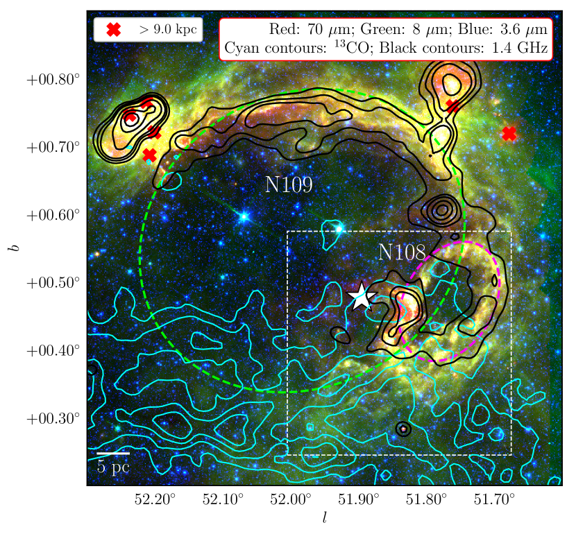
Figure 5.— Three-color composite image of the G51 region. The position of the W–R star, 1697–38F, is marked by a white star. This region also hosts two MIR bubbles, N108 and N109, which are marked by dashed blue and green ellipses, respectively. The 1.4 GHz VGPS contours (in black) are marked at levels of 11, 13, 15, 21, 30, and 40 mJy beam^-1. Cyan contours correspond to the integrated ¹³CO gas of the possible host molecular cloud toward the region. The remaining symbols are similar to those in Figure 1.

Several authors reported that the H ii regions associated with the bubbles are located at a far kinematic distance of 9.8$\pm$0.5 kpc (Watson et al., 2003; Anderson et al., 2009; Bania et al., 2012). Dust clumps identified by Urquhart et al. (2018) are overplotted in Figure 5. But dust clumps are only found toward the upper edge of N109, and those clumps are located at distances greater than 9 kpc (Urquhart et al., 2018). No dust clumps are identified around the W–R star. The host molecular cloud also shows no association with these particular clumps (see Figure 5). Thus, for this region, we have selected a small 20${}^{\prime}\times$20^′ area centered at $l$=51^∘.840, $b$=+0^∘.410 for further analysis, excluding the clumps located at distances $>$9 kpc.

2.6. Reference region: G27.323–0.144

The G27.323–0.144 region (hereafter G27) hosts the MIR bubble N46 (see Figure 6a). The area (24${}^{\prime}\times$17^′) studied by Dewangan et al. (2016) is marked by a dashed box in Figure 6a. They found that the presence of the W–R star, 1503-160L, has played an important role in the formation of young stellar objects (YSOs) in this region. Several signatures of the presence of the W–R star are adopted as references for the study of our selected regions.

Table 1Details of the selected regions with parameters of the associated W–R stars and molecular clouds.

Region	Associated W–R Star						Associated molecular cloud
Gll.lll+b.bbb	RA (J2000)	Dec (J2000)	Spec.	$A_{K}$	Distance		Vel. range	Trough Vel.	Near KDa	Far KD	$v_{\mathrm{exp}}$
	(hh:mm:ss.s)	(dd:mm:ss.s)	Type	(mag)	(kpc)		(km s-1)	(km s-1)	$d\pm$1$\sigma$ kpc	$d\pm$1$\sigma$ kpc	km s-1
G15.010–0.570	18:19:22.2	–16:03:12.4	WN7o	0.56	2.3${}^{+1.3}_{-0.6}$b		20–38	29.0	2.8$\pm$0.3	13.2$\pm$0.4	4.0$\pm$1.8
G24.750+0.100	18:35:47.6	–07:17:49.9	WC9	3.35	5.7$\pm$0.5		95–115	105.5	6.0$\pm$0.6	9.2$\pm$0.4	5.0$\pm$3.0
G34.260+0.169	18:53:02.6	+01:10:22.9	WC8	4.41	2.9$\pm$0.3		49–63	53.5	3.3$\pm$0.4	10.5$\pm$0.5	–
G35.598–0.032	18:56:07.9	+02:20:48.9	WC7	2.56	3.8$\pm$0.4		44–62	56.4	3.5$\pm$0.4	10.2$\pm$0.4	5.0$\pm$3.5
G51.840+0.410	19:25:18.1	+17:02:15.9	WC9	2.16	5.9$\pm$0.5		42–52	47.3	3.7$\pm$0.6	6.8$\pm$0.7	2.0$\pm$1.8
G27.323–0.144c	18:41:34.1	–05:04:01.4	WN7d	1.21d	5.2$\pm$0.5d		88–96d	92.0	5.2$\pm$0.7	9.4$\pm$0.6	3.0d

3. Data

Details of the multi-wavelength data sets used in our analysis are presented below.

3.1. Near-infrared data

NIR magnitudes of the selected W–R stars were obtained from the Two Micron All Sky Survey catalog (2MASS catalog; Skrutskie et al., 2006; Cutri et al., 2003), mainly to allow us to calculate their spectro-photometric distances.

3.2. Mid-infrared data

The MIR images (with a spatial resolution of $\sim$2$\arcsec$) and photometric magnitudes of point-like sources were obtained from the Spitzer–GLIMPSE survey archive (i.e. the GLIMPSE-I Spring ’07 highly reliable catalog; Benjamin et al., 2003) . Multiband Infrared Photometer for Spitzer (MIPS) Inner Galactic Plane Survey (MIPSGAL; Carey et al., 2005) 24 $\mu$m photometric magnitudes of point sources (Gutermuth & Heyer, 2015) are also used.

3.3. Far-infrared data

Level2_5 processed Herschel 70–500 $\mu$m images were used. The data were obtained from the ESA-Herschel science archive (P.I. S. Molinari). The Herschel images have beam sizes of 5$\farcs$8, 12$\arcsec$, 18$\arcsec$, 25$\arcsec$, and 37$\arcsec$ at 70, 160, 250, 350, and 500 $\mu$m, respectively (Griffin et al., 2010; Poglitsch et al., 2010). These multi-band images helped us to construct column density maps with a final spatial resolution of 37$\arcsec$.

3.4. Molecular line data

To perform a detailed investigation of the molecular gas associated with the selected regions, we obtained ¹³CO ($J$=1–0) line data from the GRS (Jackson et al., 2006). GRS line data have a velocity resolution of 0.21 km s^-1, with an angular resolution of 45$\arcsec$. The data have a main beam efficiency ($\eta_{\rm mb}$) of $\sim$0.48, with a typical rms sensitivity (1$\sigma$) of $\approx 0.13$ K and a velocity coverage from $-$5 to 135 km s^-1 (Jackson et al., 2006).

In addition, we used ¹²CO ($J$=1–0), ¹³CO ($J$=1–0), and C¹⁸O ($J$=1–0) line data from the FOREST (i.e. the four-beam receiver system on the Nobeyama 45 m telescope; Minamidani et al., 2016) unbiased Galactic plane imaging survey (FUGIN; Umemoto et al., 2017). The 45 m radio telescope is operated by the Nobeyama Radio Observatory. The FUGIN survey data cover the Galactic longitude ranges 10^∘–50^∘ and 198^∘–236^∘. The data have a velocity resolution of 1.3 km s^-1 and an angular resolution of 21^′′, with a (1$\sigma$) rms sensitivity of 0.12 K.

3.5. Radio continuum data

To examine the distribution of the ionized gas, we retrieved the VGPS 1.4 GHz continuum maps. The VGPS maps have an angular resolution of 60^′′ and an rms of 11 mJy beam^-1 (Stil et al., 2006). In addition, to identify the detailed structures of the ionized gas, we also used the 1.4 GHz continuum maps from National Radio Astronomy Observatory (NRAO) Jansky Very Large Array (VLA) Sky Survey (NVSS) as it provides a better angular resolution with a beam size of $\sim$45^′′ and a sensitivity of $\sim$0.45 mJy beam^-1 (Condon et al., 1998).

4. Search for molecular clouds associated with W–R stars

Identification of the host molecular clouds and establishing their association with W–R stars is essential before proceeding to search for any possible influence of the W–R stars. Thus, we first determined the distances to the selected W–R stars, and the molecular clouds in the velocity range of the dust clumps (see Section 2) in order to establish their possible association. We considered a molecular cloud to be the host cloud of a W–R star if the kinematic distance of that cloud is matched with the distance of the W–R star within an uncertainty of 1$\sigma$.

4.1. Distances to W–R stars

The only W–R star in our sample that has Gaia parallax measurements is the one in the G15 region. Thus, the distances to the remaining W–R stars in our sample are determined using the spectro-photometric method following Shara et al. (2012). For completeness, the procedure is briefly outlined here. Crowther et al. (2006) extensively studied the W–R star population in the cluster Westerlund 1, and reported the absolute magnitudes of W–R stars of different spectral types. Spectro-photometric distances to W–R stars in our sample were estimated after correcting for foreground extinction following a similar procedure as adopted by Dewangan et al. (2016). Estimated values of the extinction and distance to each W–R star are listed in Table 1. However, for the W–R star in the G15 region, we used the distance from Gaia astrometry (Bailer-Jones et al., 2018).

4.2. Identification of molecular clouds associated with W–R stars

In this section, we identify those molecular clouds that have similar distances as the W–R stars and thus, could be physically associated with each other. We first look for the molecular clouds that overlap with the $v_{\mathrm{LSR}}$ of the ATLASGAL dust clumps reported by Urquhart et al. (2018). Also, because of strong energetics, these W–R stars are able to develop cavities in their parent molecular clouds. Once such a cavity develops, its signature could also be present in the corresponding ¹³CO spectrum if the molecular gas still exists in the foreground and background of the W–R star. In this scenario, ¹³CO spectrum toward the W–R star should show a double-peaked emission profile separated by a few km s^-1. The velocity corresponding to the position of the W–R star should fall in the trough between the double-peaked emission features (i.e. the part of the cloud devoid of molecular gas). The separation between the two emission peaks depends on the age and wind velocity of the driving W–R star and also on the initial density of the surrounding molecular cloud.

Figure 6b shows the ¹³CO spectrum of the G27 region. The molecular cloud hosting this particular region is located at a velocity range of 88–95 km s^-1 (see Dewangan et al., 2016). The spectrum is constructed by combining all ¹³CO emission within a 45^′′ diameter (i.e., the beam size of the GRS data) centered on the W–R star. Two emission peaks are clearly visible in the spectrum. We estimated the kinematic distance corresponding to the velocity of the trough ($v_{\mathrm{LSR}}~{}\sim~{}$92.0 km s^-1; see Figure 6b) using the ‘Kinematic Distance Calculation Tool’ of Wenger et al. (2018) which evaluates a Monte Carlo kinematic distance adopting the solar Galactocentric distance of 8.31$\pm$0.16 kpc (Reid et al., 2014). The calculation yields a near kinematic distance ($d_{\mathrm{Near}}$) of 5.2$\pm$0.6 kpc.

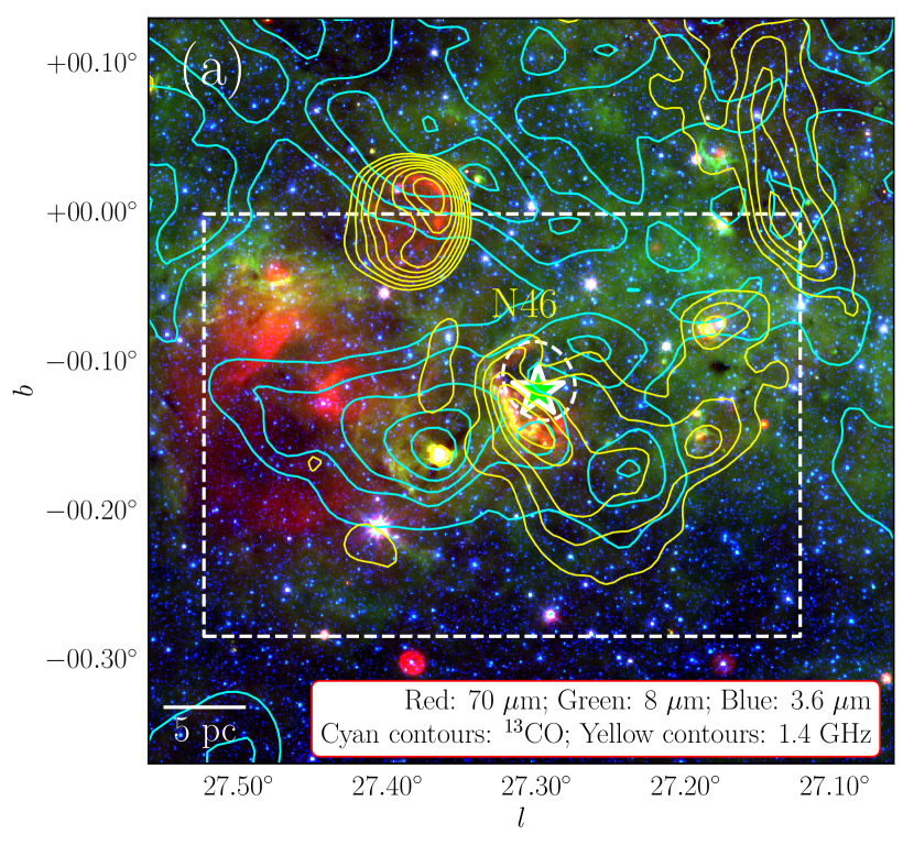
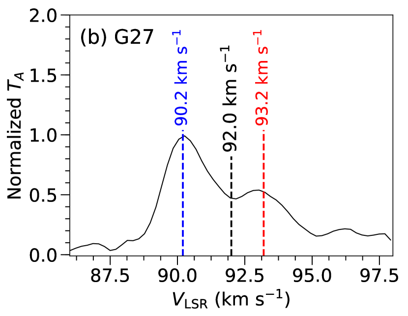
Figure 6.— Three-color composite image of the reference region, G27. The position of the W–R star, 1503–160L, is marked by a green star. The region hosts a MIR Galactic bubble, N46, which is marked by a dashed white ellipse. The 1.4 GHz VGPS contours (in yellow) are overplotted at levels of 28, 32, 37, 43, 50, 58, 70, and 90 mJy beam^-1, and cyan contours show the distribution of ¹³CO gas. A scale bar corresponding to 5 pc is shown in the bottom left-hand corner. (b) ¹³CO spectrum toward the W–R star in the reference region. The spectrum was obtained by averaging all emission within a circle of a 45^′′ diameter centered on the coordinates of the W–R star. Two emission peaks are clearly seen. We have marked the velocities corresponding to the emission peaks and the trough by blue and red, and black dashed lines, respectively.

The spectro-photometric distance of the W–R star associated with the reference region is 5.2$\pm$0.5 kpc (Dewangan et al., 2016, see also Table 1). A well-matched distance of a W–R star with the velocity of the trough in the ¹³CO spectrum implies a physical association of the W–R star with this particular molecular cloud and, more precisely, with the trough at a $v_{\mathrm{LSR}}$ of 92.0 km s^-1. The ¹³CO spectrum (Figure 6b) also exhibits two emission peaks corresponding to blue-shifted (90.2 km s^-1) and red-shifted (93.2 km s^-1) parts of the cloud, possibly dispersed by the energetics of the W–R star. Evidence of the influence of the W–R star was already found for this region by Dewangan et al. (2016). Hence, any region with a double-peaked ¹³CO spectrum toward the position of a W–R star exhibiting a trough might be explored for any impact of W–R stars on their parent molecular clouds.

The ¹³CO spectra for our selected regions are constructed by integrating all emission within a 45^′′ diameter, centered on the positions of the W–R stars (Figure 7) for velocity ranges where dust clumps are generally identified (see Section 2). All spectra show similar double-peaked spectral signatures as seen in the spectrum toward the reference region (see Figure 6b) except for the G34 region. The spectrum for the G34 region constructed for a 45^′′ diameter shows three peaks (see Figure 7c). However, the highest velocity peak (at $v_{\mathrm{LSR}}$ of $\sim$61 km s^-1) dissolves when the spectrum is produced for a 240^′′ diameter. This implies a small component of molecular gas along the sight line to the W–R star which is peaking at a $v_{\mathrm{LSR}}$ of 61 km s^-1. The emission peaks, troughs, and corresponding velocities are marked and labeled in Figure 7.

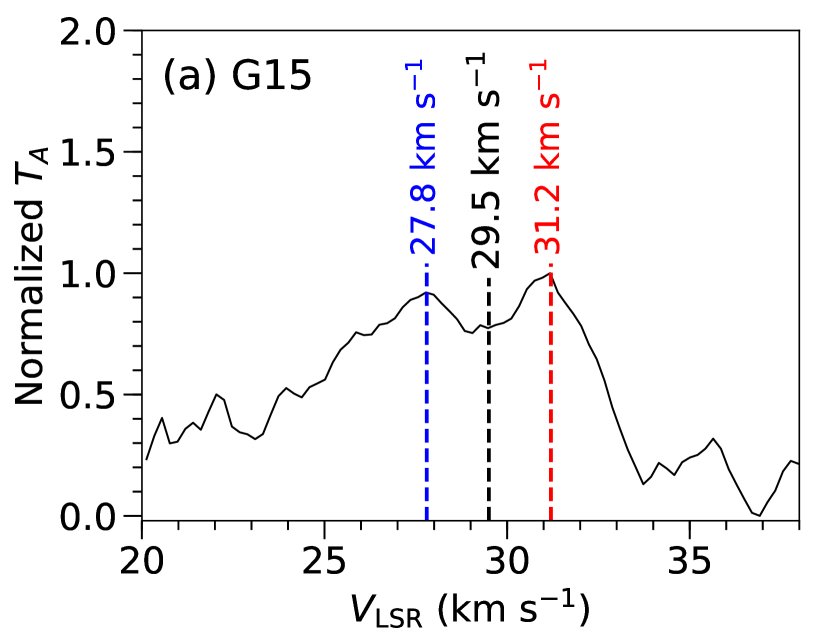
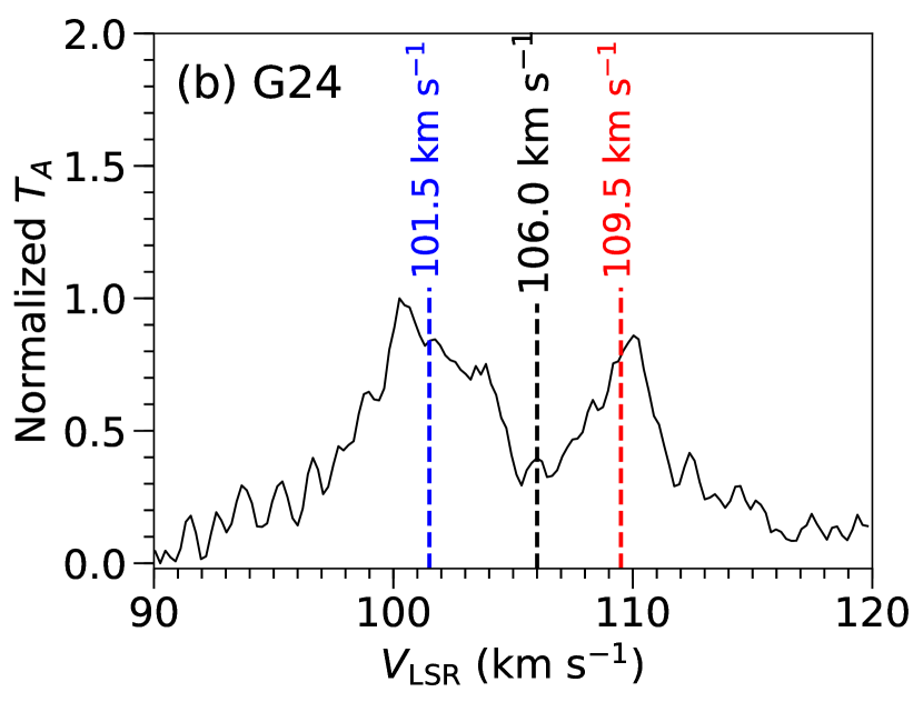
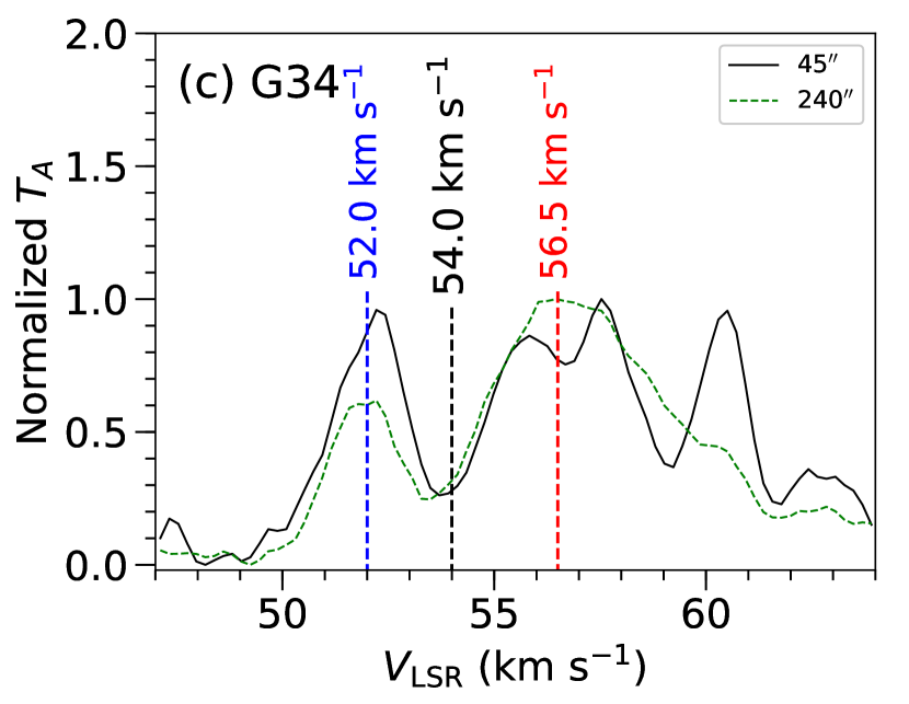
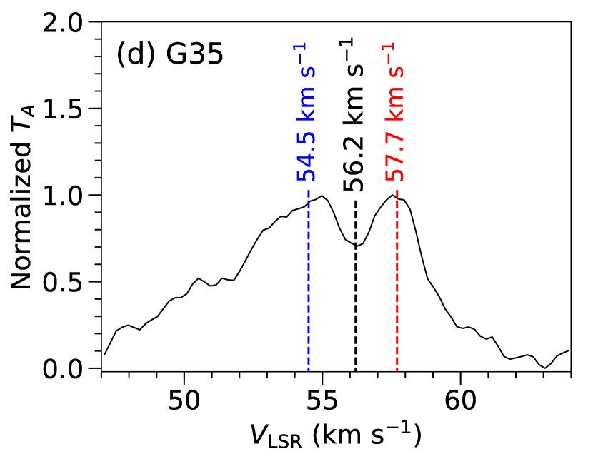
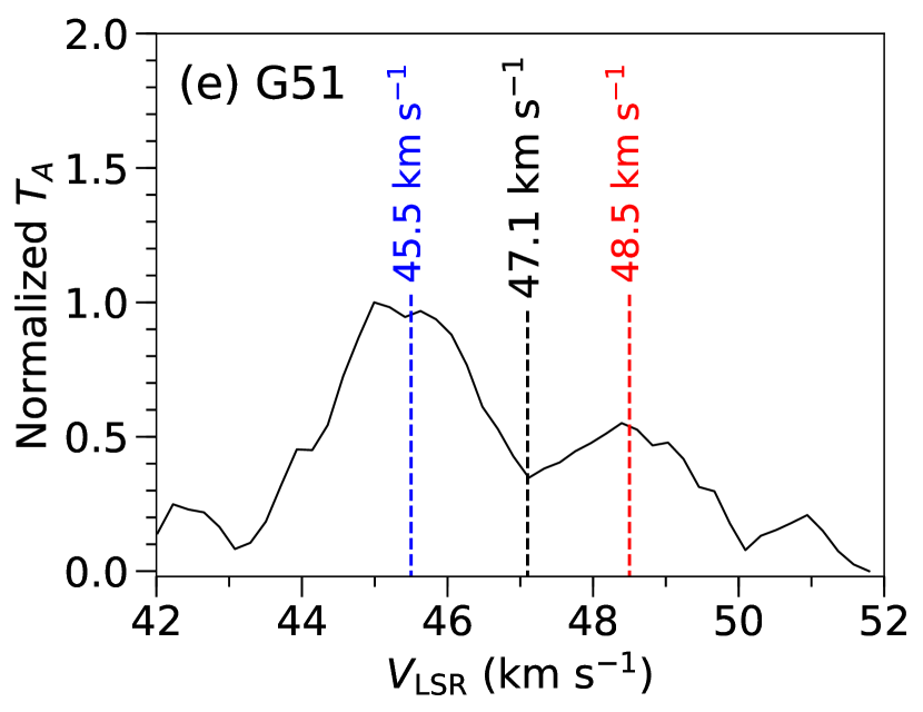
Figure 7.— ¹³CO spectra of our five selected regions (a) G15, (b) G24, (c) G34, (d) G35, and (e) G51. The spectra were constructed following the same procedure as that applied to the reference region, G27 (see the caption of Figure 6). Velocities corresponding to the blue- and red-shifted emission peaks, and to the trough, are marked by blue and red, and black-dashed lines, respectively. The ¹³CO spectrum of the G34 region constructed for a 45^′′ diameter shows three peaks. The third peak at $\sim$61 km s^-1 dissolves if the spectrum is constructed for a 240^′′ diameter.

The kinematic distances (i.e. $d_{\mathrm{Near}}$) of all but one trough (in the G51 region) agree well with the distances of the respective W–R stars, indicating that they are the host clouds of these W–R stars (see Table 1 for the velocity ranges of the identified clouds). The scenario is different for G51 as no dust clumps were identified near the W–R star in this region (Urquhart et al., 2018). Upon exploring the GRS ¹³CO spectrum for the entire observed velocity range, we identified a molecular cloud in a velocity range of 43–51 km s^-1 with the expected double-peaked spectral signature (Figure 7e). For this region, the $d_{\mathrm{Far}}$ (6.8$\pm$0.7 kpc) corresponding to the velocity of the trough lies within the range of the spectro-photometric distance (5.9$\pm$0.5 kpc) of the W–R star. It is also possible for this region that the surrounding area of this W–R star is devoid of molecular gas. However, we consider that the W–R star toward the G51 region is possibly associated with this particular molecular cloud located in the $v_{\mathrm{LSR}}$ range of 43–51 km s^-1.

Note that double peaked structures in the molecular spectra may arise for several reasons. Thus, we explored the molecular spectra of five lines of sight within the field for each region presented in Appendix A. Such structures are indeed present in the molecular spectra including in the spectrum toward the W–R star in G24, but at a different $v_{\mathrm{LSR}}$ range. However, the origin of such structures is better clarified based on a position–velocity ($p-v$) analysis. All field regions that show double-peaked spectral features typically have two cloud components along the line of sight. However, the $p-v$ analysis revealed that those clouds (except for one) do not exhibit the signature that resembles the expansion of the molecular gas (unlike the signatures discussed in the next section). Only one field region (in the G24 field) shows a signature of expanding molecular gas, possibly driven by an intermediate mass YSO (for details see Appendix A).

5. Kinematics of molecular gas and identification of young sources

In the previous section, analysis of the molecular spectra helped us to identify the host clouds of all five W–R stars. In the subsequent sections, we explore the dynamics of the host molecular clouds and also search for signatures of active star formation (i.e. the presence of cold clumps and YSOs) around these W–R stars.

5.1. Dynamics of the molecular gas

The $p-v$ diagram of molecular line data (e.g., ¹³CO) is a powerful tool to probe the dynamics of the molecular gas. Expansion, inflows, and outflows in molecular clouds have different imprints in the $p-v$ diagram (see e.g. Arce et al., 2011; Dewangan et al., 2016; Baug et al., 2018). For example, ring-like, U-like, or inverted U-like structures in the $p-v$ diagram are typically indicative of the presence of expanding molecular shells (see Arce et al., 2011; Fontani et al., 2012; Feddersen et al., 2018). In the G27 region, Dewangan et al. (2016) reported the presence of an expanding molecular shell inferred from a similar feature in the $p-v$ diagram. They also estimated that the molecular shell in the G27 has an expansion velocity ($v_{\mathrm{exp}}$) of 3 km s^-1.

The integrated intensity maps and the corresponding $p-v$ diagrams of all five regions are shown in Figures 8–10. Ring-like structures are seen in the $p-v$ diagrams of all but one region (see the magenta lines in Figures 8–10). The coordinates of the W–R stars (i.e. $l$ or $b$) and the velocities of the corresponding troughs are also marked in all $p-v$ diagrams. No significant feature is seen in the G15 region when the $p-v$ diagram is constructed for the full selected area (see Figure 8b,c). But, a clear ring-like structure can be discerned when it is constructed for a 6${}^{\prime}\times$6^′ area centered on the W–R star. This could be because the $p-v$ analysis for the larger area includes strong ¹³CO emission from M17, which may drown out weak (e.g., ring-like) features. These ring-like structures in the $p-v$ diagrams are typical signatures of the presence of expanding molecular shells, and the presence of a W–R star toward the center of this ring-like structure indicates that the expanding shell has possibly developed from the influence of the W–R star.

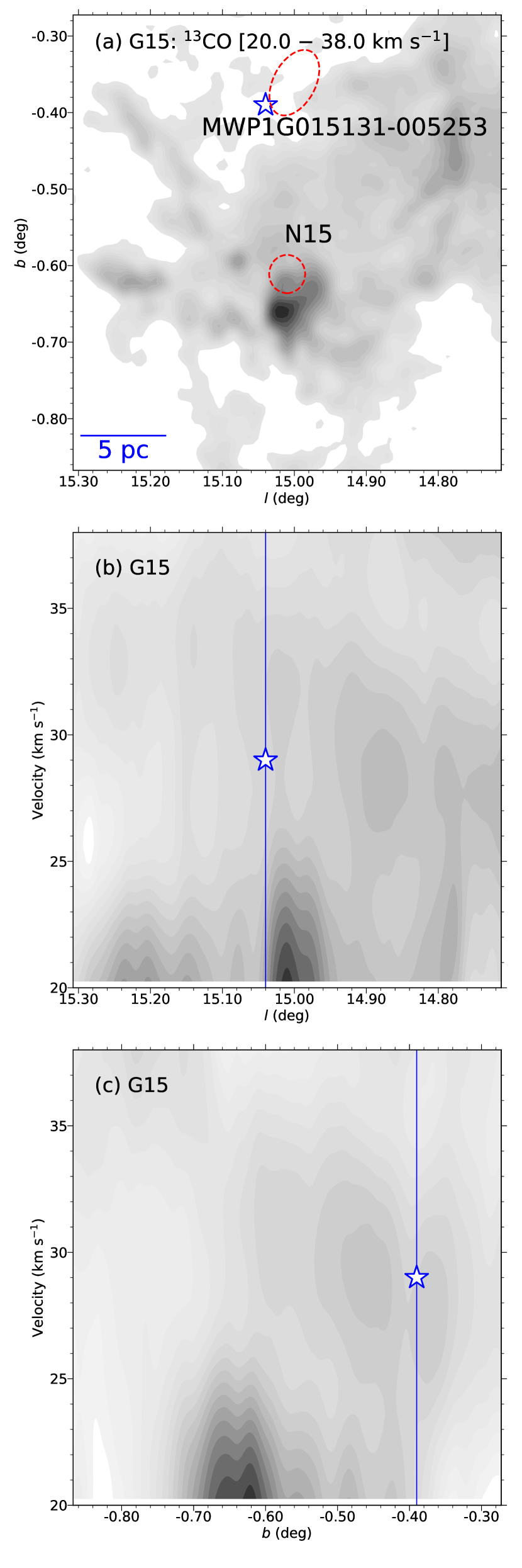
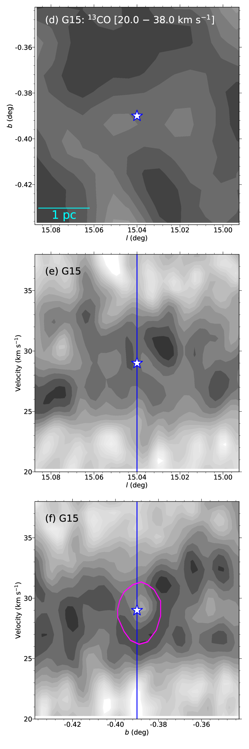
Figure 8.— (a) Integrated intensity map (solid gray contours) of the G15 region for the 36${}^{\prime}\times$36^′ area around $l$=15^∘.010, $b$=$-$0^∘.570, for a velocity range of 20–38 km s^-1. (b) and (c) Corresponding $p-v$ diagrams (solid gray contours) of the selected area around the G15 region for the same velocity range. No special feature is visible in the $p-v$ diagrams. (d), (e), and (f) are, respectively, the integrated intensity map and $p-v$ diagrams (solid gray contours) of the G15 region for the same velocity range of 20–38 km s^-1 but for a smaller area of 6${}^{\prime}\times$6^′ area around $l$=15^∘.040, $b$=$-$0^∘.390. A ring-like structure can be easily discerned in panel (f). The position of the W–R star is marked by stars in the spatial maps and by lines in all $p-v$ diagrams. The stars marked in the $p-v$ diagrams indicate the probable positions of the W–R star if it is located in the trough marked in Figure 7a.

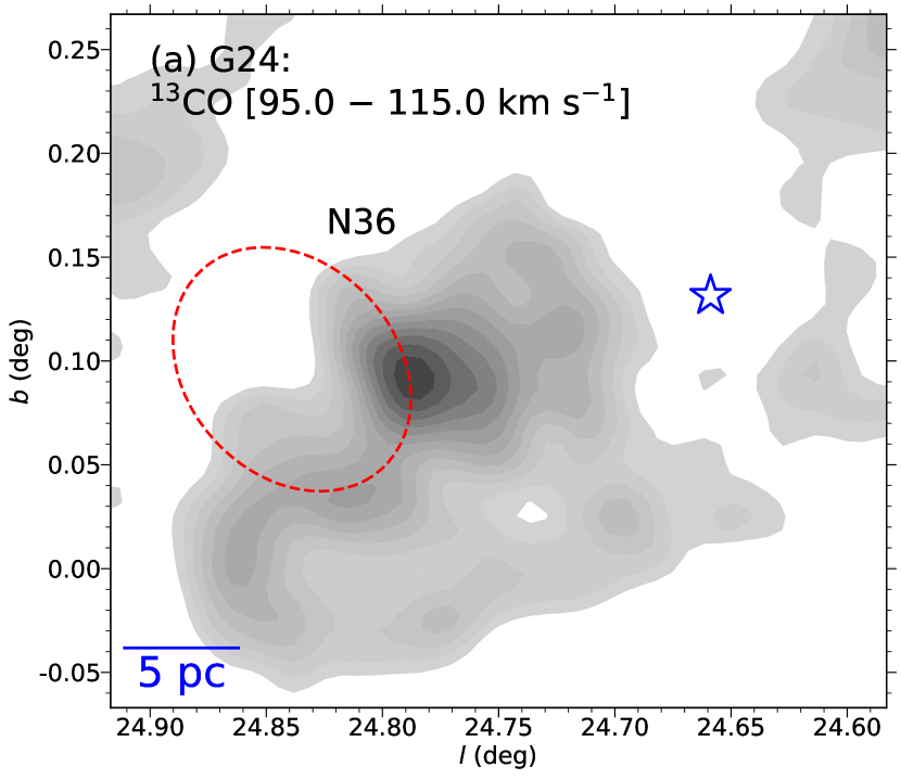
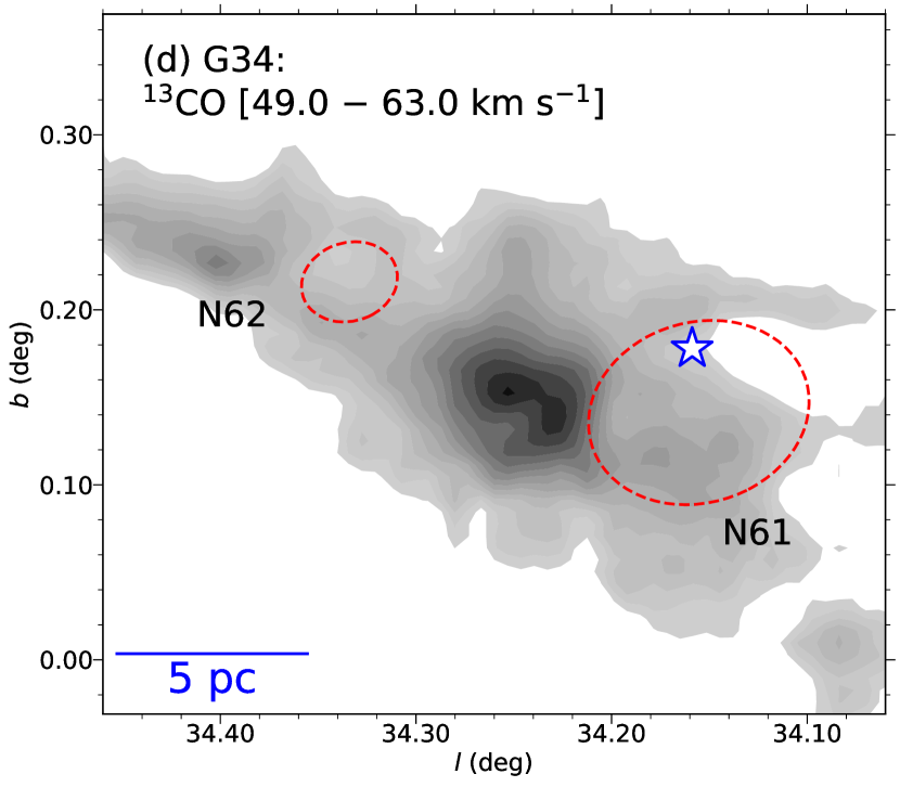
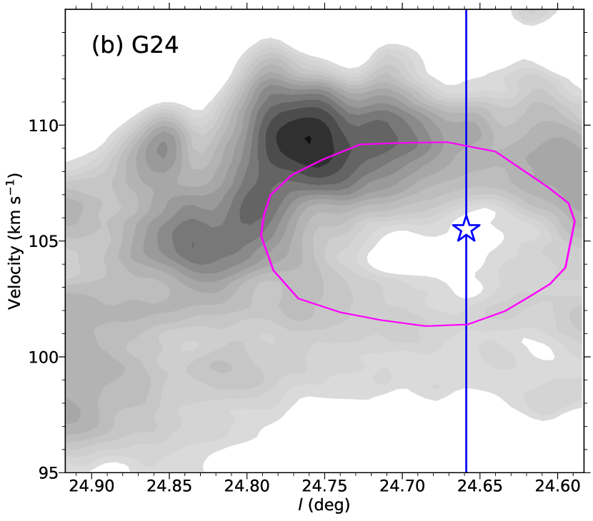
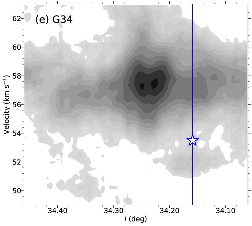
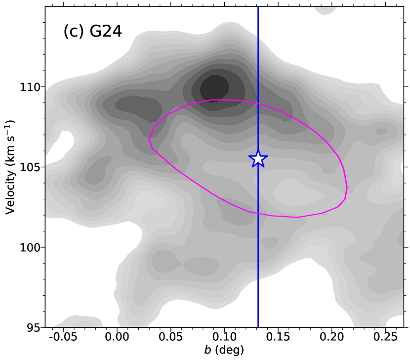
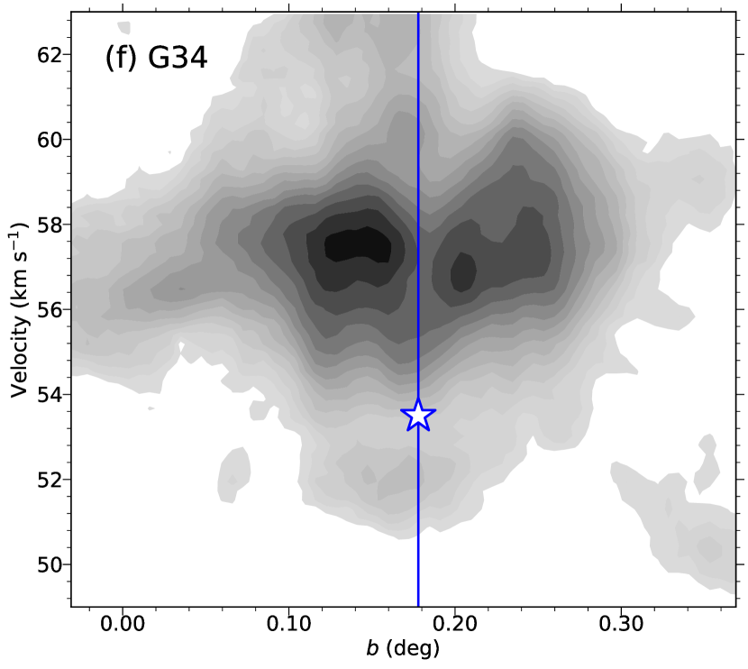
Figure 9.— (a) Integrated intensity map (solid gray contours) of the G24 region for a velocity range of 92–118 km s^-1. (b) and (c) $p-v$ diagrams (solid gray contours) of the G24 region for the same velocity range. (d), (e), and (f) are, respectively, the integrated intensity map and $p-v$ diagrams (solid gray contours) of the G34 region for a velocity range of 49–63 km s^-1. The positions of the W–R stars are marked by stars in the spatial maps and by lines in the $p-v$ diagrams of both regions. The stars marked in $p-v$ diagrams indicate the probable positions of the W–R stars if they are located in the troughs marked in Figures 7b and c.

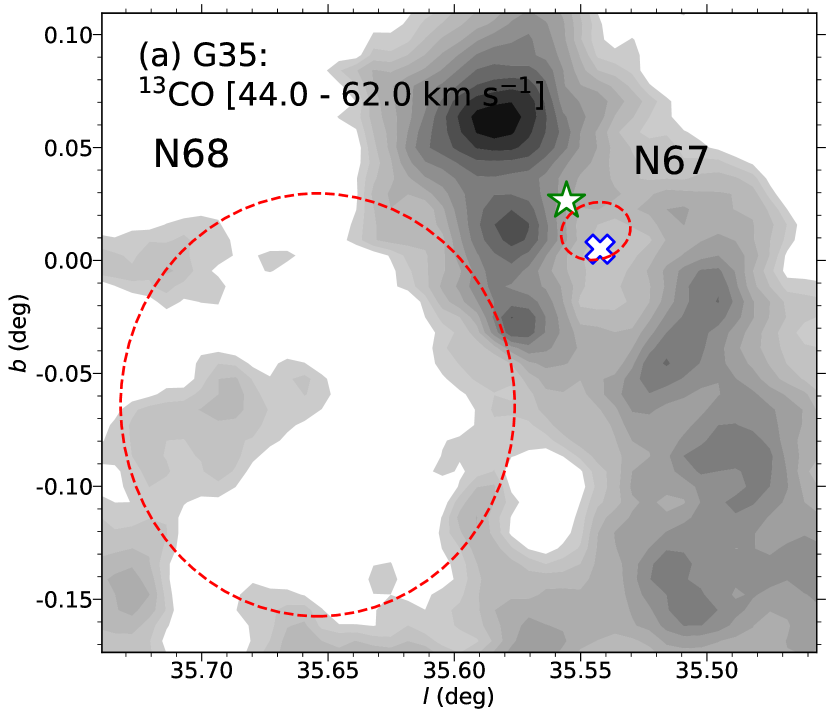
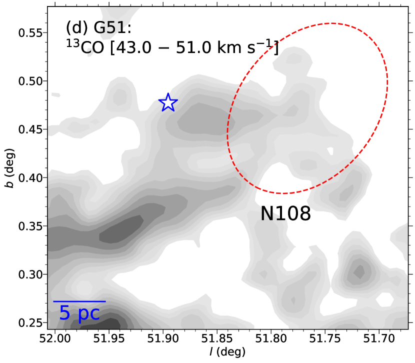
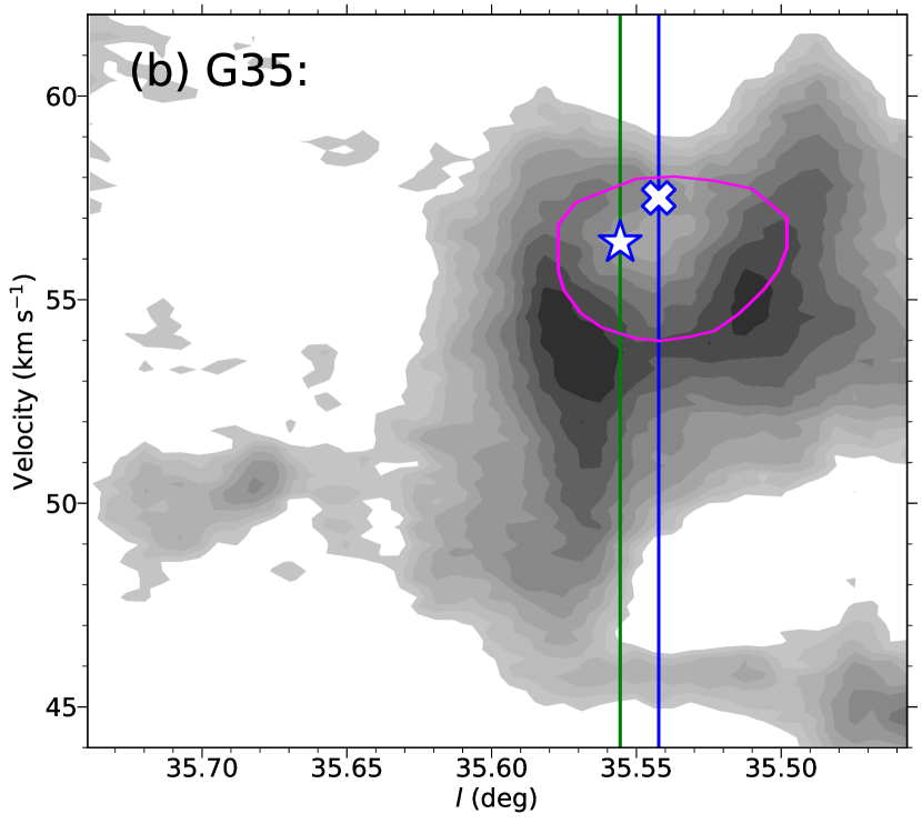
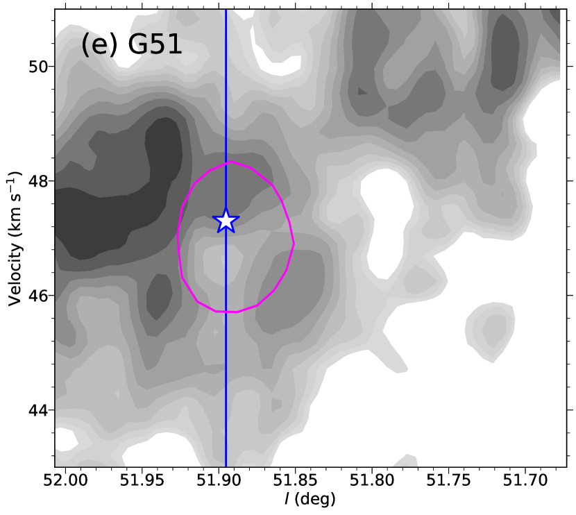
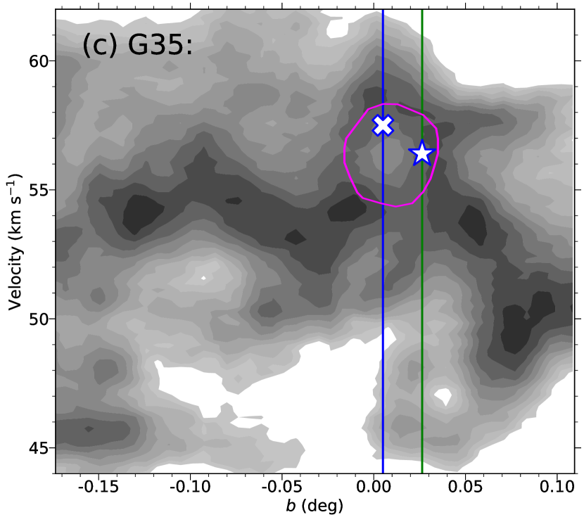
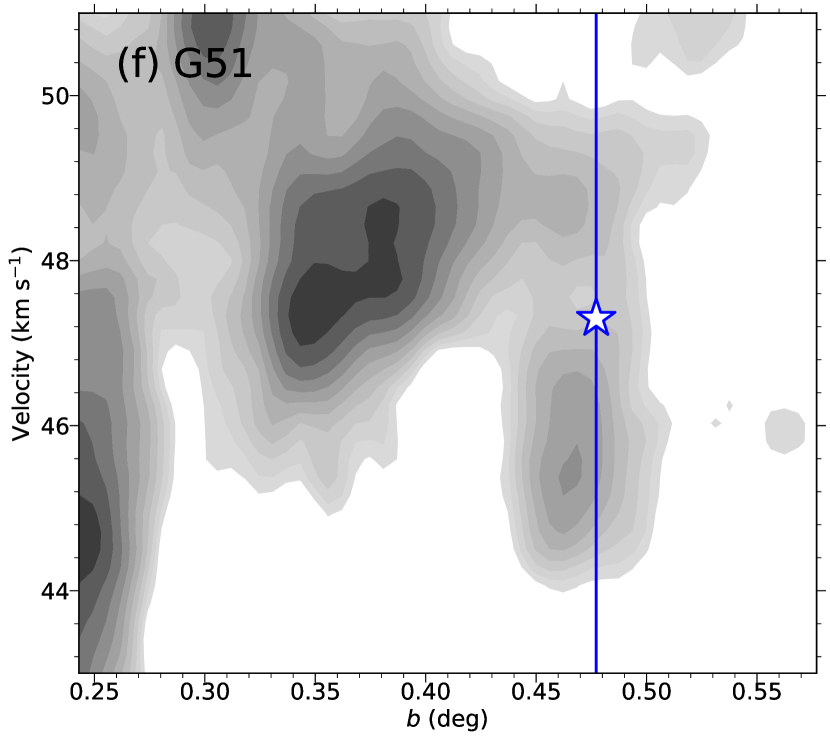
Figure 10.— (a), (b), and (c) Integrated intensity map and $p-v$ diagrams (solid gray contours) of the G35 region for a velocity range of 44–62 km s^-1. (d), (e), and (f) Integrated intensity map and $p-v$ diagrams (solid gray contours) of the G51 region for a velocity range of 42–52 km s^-1. The positions of the W–R stars are indicated by stars in the spatial maps and by lines in the $p-v$ diagrams for both regions. The stars marked in the $p-v$ diagrams indicate the probable positions of the W–R stars if they are located in the troughs marked in Figures 7d and e. Toward G35, an H ii region located near the W–R star which could also be the driving source of the expanding shell. Possible location of the H ii region is also marked by a cross in the integrated map as well as in the $p-v$ diagrams.

No ring-like or U-like structures are seen in the $p-v$ diagram of the G34 region despite the physical association of the W–R star with the corresponding molecular cloud. A possible reason could be that the red-shifted part of the cloud is larger and more intense than its blue-shifted counterpart (see Figure 7c). Thus, the red-shift cloud has sufficient intensity to surpass the faint features in the $p-v$ diagram. Note that the ring-like structure in the $p-v$ diagram of the G24 region is deformed. Also, in the G35 region, the W–R star is not exactly at the center of the ring-like structure. As can be seen in the integrated ¹³CO map of the G24 region (see Figure 9a), the molecular gas is mainly concentrated near the bubble N36. Such an asymmetrical distribution of molecular gas may lead to a deformed ring-like structure in the $p-v$ diagrams. The displacement of the W–R star with respect to the ring-like structures may arise either from differential expansion of the blue- and red-shifted parts of the molecular cloud because of their density contrast, or if the W–R star has a differential motion with respect to the surrounding clouds. For example, the cloud toward the N36 bubble with respect to the W–R star is about 3–4 times more intense compared to the cloud in the other side of the W–R star. Such contrast in the molecular cloud density cloud deform the ring-like features in the $p-v$ diagram.

For G35, an H ii region was spatially found toward the ring-like structure. However, $v_{\mathrm{exp}}$ of this particular ionized gas is 57.5$\pm$0.1 km s^-1 (Anderson et al., 2011), and hence, does not appear at the center of the ring-like structure in the $p-v$ diagram (see Figure 10a,b,c). It is, thus, possible that both W–R star and ionized gas played important role in expanding the surrounding gas. However, the dynamical age of this H ii region is ($\sim$0.5 Myr; calculated in Section 6) much lower compared to the age of the W–R star ($\sim$5 Myr). Thus, we consider that the W–R star is the primary driving source of the expanding gas. It is also possible that the W–R star in the G35 region has a differential plane of the sky motion with respect to the surrounding molecular cloud which has made it to appear off-centered. We found that in a life-time of a W–R star ($\sim$5 Myr) a differential motion of 10 $\mu as$ yr^-1 may lead to the off-set seen in the $p-v$ diagram of the G35 region. Understanding the origin of this scenario requires a detailed analysis of the proper motion of the W–R star as well as of the surrounding stars that are formed in the same host cloud. The expansion velocities of the molecular shells, inferred from the difference between the central velocity and the velocity of the outer edge of the ring-like structures, are also estimated for all regions (see Table 1). The shells identified here are expanding with velocities of 2–5 km s^-1.

5.2. Identification of dust clumps

Multiband Herschel images (160, 250, 350, and 500 $\mu$m) are useful to construct column density maps. The detailed procedure to construct a column density map is not presented in this paper but can be found elsewhere (Mallick et al., 2015; Baug et al., 2018). Figures corresponding to the column density maps are not shown here. For clump identification, we employed the python-based astrodendro package (Rosolowsky et al., 2008), which uses the dendrogram technique to identify hierarchical structures (or clumps). We considered only those clumps as real clumps that have effective areas of more than 9 pixels of column density maps and peak flux levels in excess of 5$\sigma$ compared to the surrounding background flux (where $\sigma$ is rms determined from dark patches in the maps). The traditional clumpfind method (Williams et al., 1994) was also applied to the same set of column density maps, and we found that the number of detected clumps and their central coordinates are generally similar. Henceforth, we will only consider those clumps that were identified using the dendrogram method. Statistics of the identified clumps in all five regions are presented in Table 2.

The mass of each clump is estimated using (see also Mallick et al., 2015):

$$M_{\mathrm{clump}}=\mu_{\mathrm{H_{2}}}m_{\mathrm{H}}Area_{\mathrm{pix}}\Sigma N(\mathrm{H_{2}}),$$ (1)

where $Area_{\mathrm{pix}}$ is the area subtended by a single pixel. Identified clumps have a wide range of masses (see Table 2). The dust clumps identified toward the G24 region are generally one order of magnitude more massive compared with the other four regions. Note that this particular region is located at a greater distance and, hence, multiple small clumps may appear as a single clump because of resolution limitations. Also, multiple clouds are present toward the G24 region (as seen in the ¹³CO spectrum for the full GRS velocity range). Thus, flux from multiple clouds may increase the flux levels in the Herschel maps and, hence, the estimated column density.

5.3. Young stellar sources

Young star-forming regions are typically associated with large numbers of YSOs. YSOs in all selected regions are identified using the MIR color–magnitude and color–color schemes. The Spitzer-IRAC and MIPS point sources are employed to identify and classify YSOs using [3.6]$-$[24]/[3.6] color–magnitude, and [5.8]$-$[8.0]/[3.6]$-$[4.5] and [3.6]$-$[4.5]/[4.5]$-$[5.8] color–color schemes (the corresponding figures are not shown). The detailed procedure of YSO identification schemes can be found in Baug et al. (2016). The methods used may suffer from significant contamination in distant regions, since multiple sources may appear as a single source because of the limited spatial resolution of the Spitzer images. In addition, AGB stars and background galaxies often appear with excess flux in the MIR bands, and thus, may mimic as YSOs. However, here our main interest is to statistically identify areas with active star formation rather than characterize the properties of individual YSOs. Thus, even for distant regions, these schemes may help us to identify areas with ongoing star formation. The statistics of the identified YSOs for all regions are listed in Table 2.

Table 2Details of the identified cold clumps, YSOs, and Gaia sources in all five regions.

Region	Number of	Clump Mass ($M_{\odot}$)			YSOs
	Clumps	Minimum	Maximum	Median	Class I	Flat Spec.	Class II
G15	70	107	3207	323	95	20	198
G24	27	701	16241	1838	92	11	168
G34	29	42	3642	390	136	17	152
G35	20	105	4095	445	57	6	55
G51	19	168	3955	337	27	10	33

5.3.1 Surface density analysis of YSOs

The distribution of YSO clusters in any star-forming region can help us characterize areas of active star formation. To examine the clustering behavior of YSOs toward our selected star-forming regions, we performed a nearest-neighbor surface density analysis of the identified YSOs, assuming that they are all located at a single distance. In surface density analysis, any value can be adopted for nearest-neighbor to examine clustering behavior. Generally, a large value of nearest-neighbor is sensitive to the large-scale distribution of YSOs, while a small value helps to identify small-scale density variations. This method can be thought of as a smoothing process to identify areas with large numbers of YSOs. We performed the nearest-neighbor surface density analysis for 20 YSOs as Schmeja et al. (2008) reported that 20 nearest-neighbor analysis can be used to identify clusters of 10–1500 YSOs. Figure 11a shows the locations of the YSOs in the G15 region overplotted on the Herschel 350 $\mu$m image. The surface density contours of Class I (including flat-spectrum sources) and Class II YSOs in the G15 region, overlaid on the integrated C¹⁸O intensity map over the velocity range 20–38 km s^-1, are shown in Figure 11b. Because of the large optical depth, C¹⁸O emission detects the densest parts of the molecular clouds compared to ¹²CO and ¹³CO. Again, we perform a dendrogram analysis on this integrated C¹⁸O map to identify cold molecular condensations. Cold condensations identified in the integrated C¹⁸O/¹³CO maps and the dust clumps (Urquhart et al., 2018) are marked in Figure 11b.

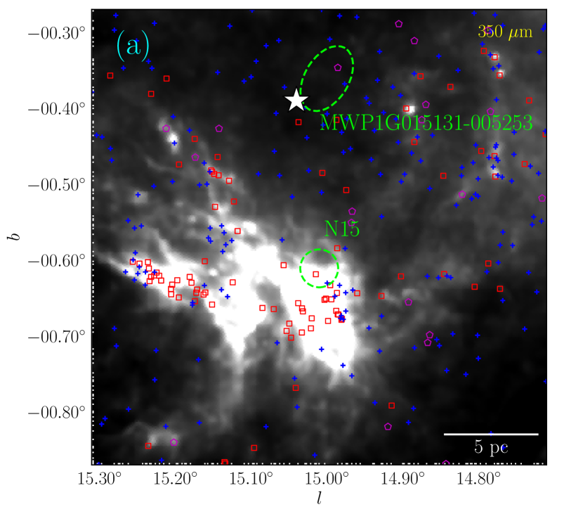
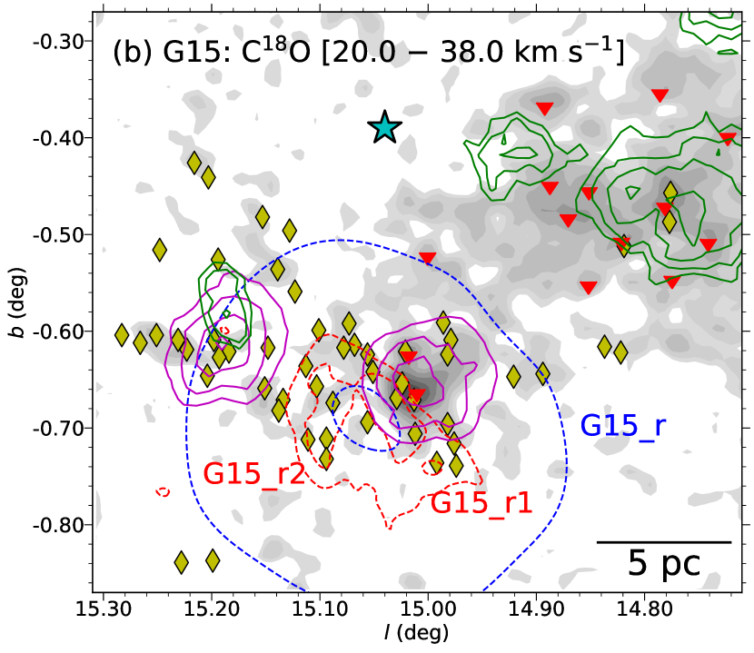
Figure 11.— (a) Class I (red squares), flat-spectrum (magenta pentagons), and Class II (blue crosses) YSOs overplotted on the Herschel 350 $\mu$m image of the G15 region. The remaining symbols are similar to those in Figure 1. (b) 20 nearest-neighbor surface density contours of Class I (and flat-spectrum) and Class II YSOs in magenta and green, respectively, are overlaid on the velocity-integrated C¹⁸O map (solid gray contours). The contours are drawn at 0.45, 0.6, 0.9, and 1.4 YSO pc^-2 for Class I and 0.45, 0.5, 0.6, 0.8 YSO pc^-2 for Class II sources. Contour at 100 and 3,000 mJy beam^-1 of the VGPS 1.4 GHz emission are also shown in dashed blue to indicate the extent of the ionized gas. The NVSS 1.4 GHz contour at 300 and 3,000 mJy beam^-1 are also shown in dashed red which resolves two peaks, and are also labeled. The corresponding ionized regions are labeled. Positions of the cold condensations and dust clumps (Urquhart et al., 2018) are shown as red triangles and yellow diamonds, respectively. The position of the W–R star is marked by a cyan star.

The 20 nearest-neighbor surface density contours for other regions, overlaid on velocity-integrated C¹⁸O maps, are shown in Figure 12. As C¹⁸O data were not available for the G51 region, the 20 nearest-neighbor YSO surface density contours for this region are overplotted on an integrated ¹³CO map. The 5$\sigma$ VGPS contours of ionized gas in all regions are also shown to mark the boundaries of the ionized gas.

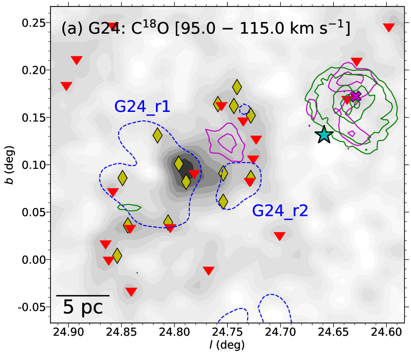
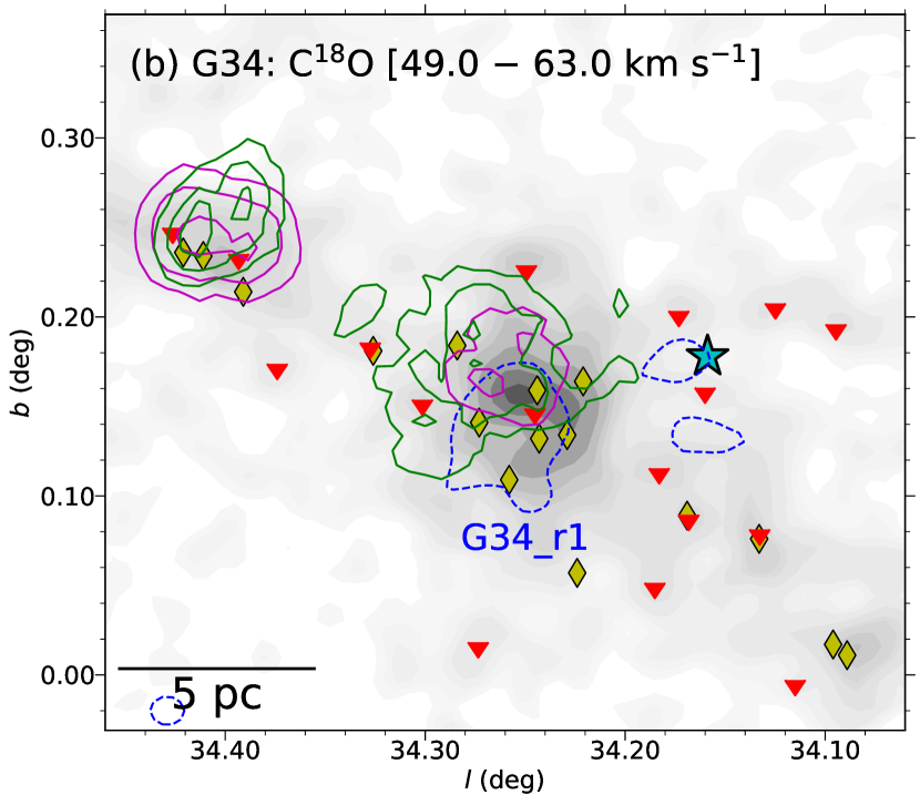
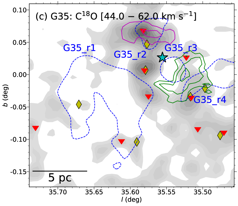
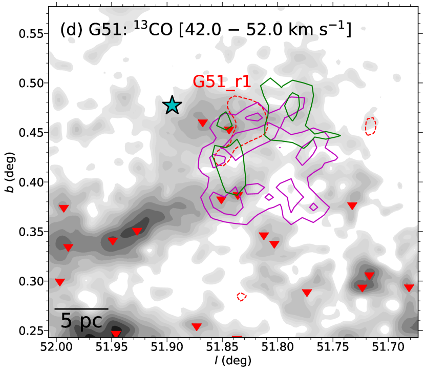
Figure 12.— The 20 nearest-neighbor surface density contours of Class I (and flat-spectrum) and Class II YSOs in magenta and green, respectively, overlaid on the velocity-integrated C¹⁸O maps (solid gray contours). As C¹⁸O data were unavailable for the G51 region, the contours for this region are overlaid on the velocity-integrated ¹³CO map. (a) G24 region: Class I contours are drawn at 0.20, and 0.25 YSO pc^-2, Class II contours at 0.25, 0.30, 0.45, and 0.60 YSO pc^-2, and a single contour of ionized gas in dashed blue at 250 mJy beam^-1 shows the extent of the ionized gas. (b) G34 region: Class I contours are drawn at 1.3, 2, and 4 YSO pc^-2, Class II contours at 0.65, 0.8, and 1.0 YSO pc^-2, and 180 mJy beam^-1 for the ionized gas. (c) G35 region: 0.4, and 0.5 YSO pc^-2 for Class I, and 0.27, 0.3, and 0.35 YSO pc^-2 for Class II, and 170 mJy beam^-1 for the ionized gas. (d) G51 region: 0.035 and 0.04 YSO pc^-2 for Class I and 0.03 and 0.035 YSO pc^-2 for Class II, and 90 mJy beam^-1 for the ionized gas. Ionized regions in all panels are labeled. Positions of cold condensations and dust clumps (Urquhart et al., 2018) are marked as red triangles and yellow diamonds, respectively. Note that no dust clumps are identified in the selected area for G51. Positions of the W–R stars are marked by cyan stars.

5.4. Molecular shells around W–R stars

Herschel column density maps are often contaminated by foreground and background emission. Such contamination becomes particularly unavoidable toward the inner Galactic plane. Although this might not affect the large structures, it could overwhelm faint structures in the Herschel column density maps. The FUGIN survey (see Section 3.4) provides simultaneously observed spectral data of the ¹²CO ($J$=1–0), ¹³CO ($J$=1–0), and C¹⁸O ($J$=1–0) lines. The ¹²CO and ¹³CO data were used to construct column density maps of the selected regions. This method to construct column density maps is expected to be more robust, because it generates maps for any given velocity range and thus eliminates foreground and background contributions. Excitation temperatures ($T_{\mathrm{ex}}$) were estimated from the ¹²CO data assuming the transition as optically thick, using

$$T_{\mathrm{ex}}=5.5/\mathrm{ln}~{}\bigg{(}1+\frac{5.5}{T_{\mathrm{mb}}(^{12}\mathrm{CO~{}peak})+0.82}\bigg{)}.$$ (2)

The corresponding $T_{\mathrm{ex}}$ was used to estimate the optical depth of the ¹³CO emission ($\tau_{13}(v)$) at each pixel and velocity ($v$) from the ¹³CO brightness temperature ($T_{\mathrm{mb}}(v)$),

$$\tau_{13}(v)=-\mathrm{ln}~{}\bigg{[}1-\frac{T_{\mathrm{mb}}(v)}{5.3}\bigg{(}\frac{1}{\mathrm{exp}(\frac{5.3}{T_{\mathrm{ex}}})-1}-0.16\bigg{)}^{-1}\bigg{]}.$$ (3)

The ¹³CO column density for each pixel was estimated by integrating the emission over the identified velocity range, using

$$N(^{13}\mathrm{CO})=2.4\times 10^{14}\times\sum\frac{T_{\mathrm{ex}}\tau_{13}(v)\Delta v}{1-\mathrm{exp}\big{(}-\frac{5.3}{T_{\mathrm{ex}}}\big{)}}.$$ (4)

Finally, $N(^{13}\mathrm{CO})$ was converted to $N(\mathrm{H_{2}})$ using a conversion factor of 7.7$\times$10⁵ (Kohno et al., 2018). A more detailed description of the calculation method can be found in Kohno et al. (2018) and Torii et al. (2019). The final column density maps for four regions are presented in Figure 13. As FUGIN data do not cover the G51 region, we used the Herschel column density map to identify the molecular shell. It is found that a few clumps seen in the dust column density maps (figures are not shown in this paper) are missing in these gas column density maps. Those clumps might be part of foreground and background clouds. In addition, gas column density maps detected detailed structures that were missing in the dust column density maps, possibly because the ¹³CO column density maps are less contaminated from the foreground and background emission.

Low-density cavities and circular shells around W–R stars are apparent in almost all regions except for G35 (see Figure 13). Note that these shells and cavities are identified around W–R stars using molecular line data, and are different from the MIR bubbles seen in the Spitzer-IRAC images. Possible inner boundaries of the shells are marked by red circles based on visual identification of the cavities. Although the shell is not very apparent in the G35 region, the immediate vicinity of the W–R star is deficient in molecular gas (see Figure 13d). The outer boundaries of the shells are also marked by white circles of radii equal to twice the radii of the inner boundaries. Note that these outer boundaries do not have any physical significance, but just help us in estimating the average column densities of the shells. The cavities within the shells are devoid of molecular gas and have comparatively lower column densities than the annular areas marked within the red and white circles.

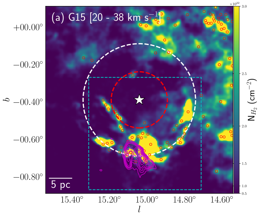
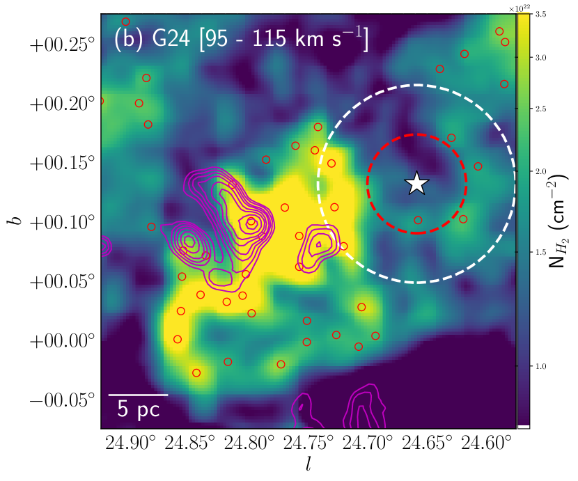
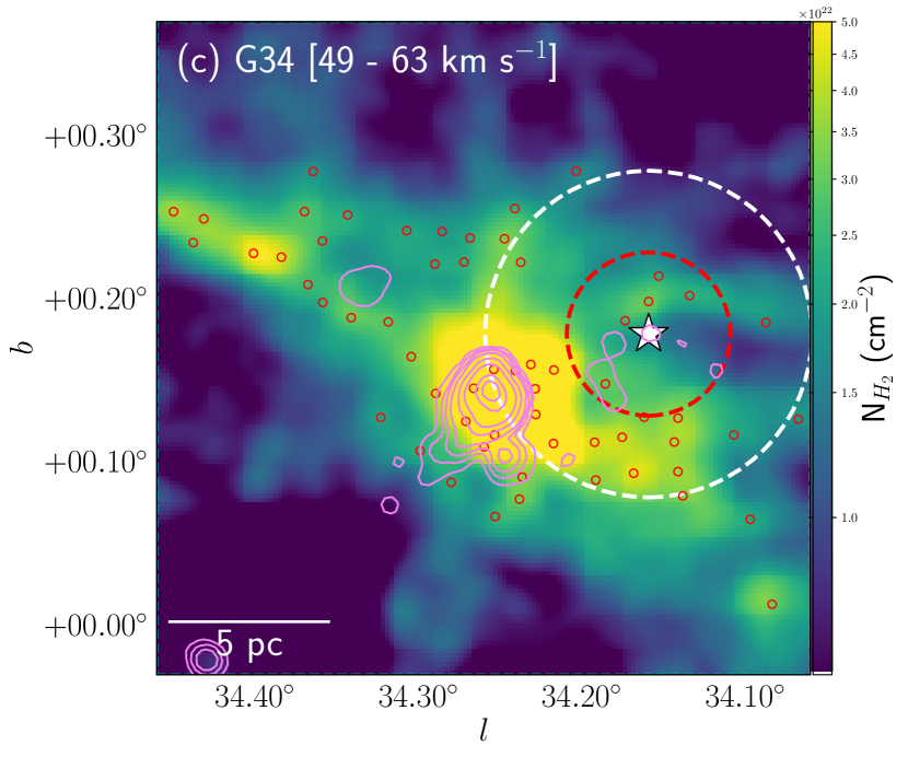
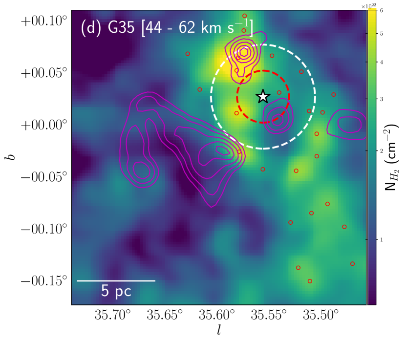
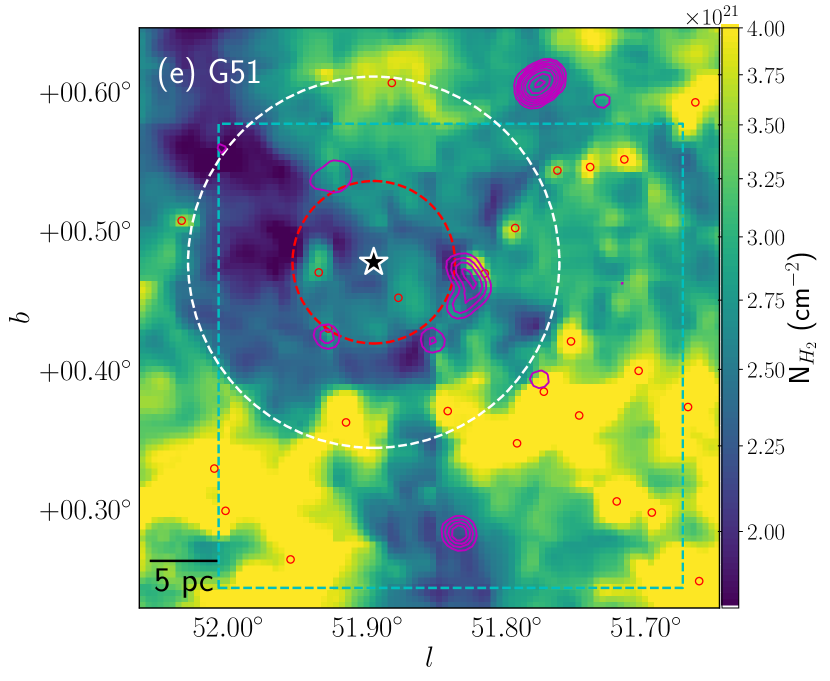
Figure 13.— Column density maps constructed using ¹²CO and ¹³CO data of all regions. Since ¹²CO data were not available for the G51 region, we show the Herschel column density map again for a larger area. The cyan dashed boxes for the G15 and G51 regions show the areas of interest. For remaining regions, maps are shown for the same areas explored in this paper. The magenta contours in each panel depict the distribution of the ionized gas. Possible boundaries of cavities centered on the W–R stars are marked as red dashed circles. Outer boundaries of shells (radii twice the radii of corresponding inner shells) are also marked as white dashed circles. The annular areas in red and white circles are meant to help us estimate the column densities of the shells. Clumps identified in these column density maps are also marked by small red open circles.

5.5. Pressure of W–R stars

We identify the primary energetic component of the W–R stars that acts as the major agent to disperse the surrounding molecular gas. The expansion of the molecular gas with velocities of about 2–5 km s^-1 is detected in the $p-v$ diagrams of all regions (except for G34; see Section 5.1) which is likely caused by the energetic inputs from the central W–R stars. In general, massive stars exert multiple pressure components on their surrounding molecular gas (e.g. pressure owing to radiation, stellar winds, and ionized gas).

To get an idea about the different pressure components and the extent of the influence of the W–R stars, we computed the pressure owing to stellar winds, $P_{\mathrm{wind}}$ ($=\dot{M_{\mathrm{w}}}V_{\mathrm{w}}/4\pi D_{\mathrm{s}}^{2}$, where $D_{\mathrm{s}}$ is the distance from the W–R star) and the pressure owing to radiation, $P_{\mathrm{rad}}$ ($=L_{\mathrm{bol}}/4\pi cD_{s}^{2}$) for a range of distances from the W–R star. Nugis & Lamers (2000) studied the wind characteristics of W–R stars based on their stellar parameters. The stellar wind velocities for our spectral types were obtained from Nugis & Lamers (2000). Typical mass-loss rates for these stars were also computed using their equation (24). Armed with those typical values of mass-loss rates ($\dot{M_{\mathrm{w}}}$) and stellar wind velocities ($V_{\mathrm{w}}$), we estimate $P_{\mathrm{wind}}$ for a separation range ($D_{\mathrm{s}}$) of 1–20 pc from the powering W–R star (see Figure 14). To calculate $P_{\mathrm{rad}}$, the bolometric luminosities ($L_{\mathrm{bol}}$) of these W–R stars are also obtained from Nugis & Lamers (2000). The $L_{\mathrm{bol}}$ values are similar ($\sim$2–5$\times$10${}^{5}~{}L_{\odot}$) for all W–R spectral types in our sample. Hence, $P_{\mathrm{rad}}$ is estimated for a single $L_{\mathrm{bol}}$ value of 3$\times$10${}^{5}~{}L_{\odot}$, for the same range of $D_{\mathrm{s}}$. Figure 14 shows that $P_{\mathrm{wind}}$ is typically an order of magnitude higher than $P_{\mathrm{rad}}$. Dyson & Williams (1980) reported that a cool giant molecular cloud with a typical temperature of $\sim$20 K and a particle density of 10³–10⁴ cm^-3 exhibits an outward pressure (i.e. $P_{\mathrm{MC}}$) of about 10^-12–10^-11 dyne cm^-2. None of the W–R stars in our sample are associated with ionized gas peaks, which makes it difficult to estimate the pressure owing to the ionized gas from W–R stars. Dewangan et al. (2016) also found for the G27 region that the pressure from ionized gas is two orders lower compared to $P_{\mathrm{wind}}$ and $P_{\mathrm{rad}}$. We nevertheless estimated a characteristic value of pressure owing to ionized gas formed by an O-type progenitor of a W–R star ($m_{\ast}\sim 20M_{\odot}$). The ionized gas pressure can be formulated as, $P_{\mathrm{HII}}=\mu_{\mathrm{II}}m_{H}c_{\mathrm{II}}^{2}\left(S_{Lyc}/4\pi\beta_{2}D_{\mathrm{s}}^{3}\right)^{1/2}$, where the mean molecular weight in an H ii region, $\mu_{\mathrm{II}}$=0.678 (Bisbas et al., 2009), the sound speed in an H ii region, $c_{\mathrm{II}}$ = 11 km s^-1, and the recombination coefficient, $\beta_{2}$ = 2.6$\times$10^-13 cm³ s^-1. Possible pressure component caused by H ii region developed by a typical O-type progenitor of a W–R star ($S_{Lyc}\sim$10^48.3 photon s^-1; Panagia, 1973) is also plotted in Figure 14. It can be seen that the pressure due to ionized gas is typically lower compared to $P_{\mathrm{wind}}$. Accordingly, in Figure 14 one can see that these W–R stars can drive the surrounding molecular gas out to a distance of about 10 pc primarily because of their stellar winds.

Table 3Parameters of the ionized gas and shells in all five regions.

Region	Cavity	$N(\mathrm{H_{2}})$ (1021cm-2)			Ionized	Int. Flux	log ($S_{\mathrm{Lyc}}$)	$R_{\mathrm{t}}$	$t_{\mathrm{dyn}}\mathrm{(}Myr)$	$P$ on shella
	size (pc)	Cavity	Shell	Inc. factorb	Region id	density (Jy)	(photon s-1)	(pc)	(5000 cm-3)	$P_{\mathrm{wind}}$	$P_{\mathrm{HII}}$
G15	6.0	9.6	18.0	88%	G15_r	571.700	50.435	4.71	0.965	14.7	27.5
	6.0	9.6	18.0	88%	G15_r1c	130.240	49.793	2.48	0.451	14.7	14.6
					G15_r2c	146.680	49.844	1.85	0.252	14.7	14.4
G24	5.0	13.9	18.2	31%	G24_r2	5.738	49.188	3.35	1.116	5.1	9.4
G34	3.0	22.2	30.0	35%	G34_r1	10.565	48.866	0.65	0.070	18.3	19.0
G35	1.3	28.0	31.8	14%	G35_r1	1.492	48.251	1.01	0.231	96.5	14.3
					G35_r2	1.797	48.332	1.36	0.373	96.5	35.6
G51	6.0	2.4	2.8	17%	G51_r1d	0.088	47.403	–	–	2.4	–

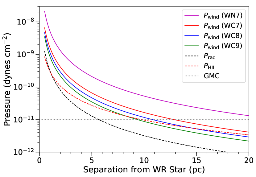
Figure 14.— Wind pressure exerted by W–R stars of different spectral types (red, green, blue, and magenta curves) at different physical distances. The pressure owing to radiation is shown by a single dashed black curve, because all WC7, WC8, WC9, and WN7 stars have a similar bolometric luminosity of about 3$\times$10${}^{5}~{}L_{\odot}$. The pressure experienced by a typical cool giant molecular cloud is shown by the gray dotted line. In the absence of ionized peaks associated with W–R stars, we have shown a possible pressure component of ionized gas (red dashed line) developed by a typical O-type progenitor ($m_{\ast}\sim 20M_{\odot}$). For all W–R stars, the pressure owing to winds is an order of magnitude higher than the radiation pressure.

Although no ionized-gas peaks are exactly associated with any W–R stars in our sample, several H ii regions are present in the selected regions. In fact, these H ii regions are spatially distributed around the molecular shells identified in Section 5.4 (see also Figure 13). Note that expansion of the ionized gas is believed to be an efficient triggering mechanism. Thus, it is important to explore the pressure exerted by these particular H ii regions ($P_{\mathrm{HII}}$) on the surrounding gas. To estimate $P_{\mathrm{HII}}$, we obtained the Lyman continuum flux ($S_{\mathrm{Lyc}}$ in photons s^-1) for selected ionized regions located near the W–R stars (see labels in Figures 11b and Figure 12) using the radio continuum flux, following the equation given by Moran (1983):

$$S_{\mathrm{Lyc}}=8\times 10^{43}\left(\frac{S_{\nu}}{\mathrm{mJy}}\right)\left(\frac{T_{e}}{10^{4}\mathrm{K}}\right)^{-0.45}\left(\frac{D}{\mathrm{kpc}}\right)^{2}\left(\frac{\nu}{\mathrm{GHz}}\right)^{0.1},$$ (5)

where $S_{\nu}$ is the total flux density, $T_{e}$ is the electron temperature, $D$ is the distance to the source, and $\nu$ is the frequency of the observations. The assumption was made that the region is homogeneous and spherically symmetric. The radio continuum fluxes and extents of the ionized regions are estimated from the VGPS 1.4 GHz maps using the jmfit task in aips. The pressure owing to ionized gas ($P_{\mathrm{HII}}$) is formulated as outlined above. The estimated radio continuum flux densities, extent of the ionized gas in pc, and $S_{\mathrm{Lyc}}$ are listed in Table 3. As ionized regions are distributed around the molecular shells, they may exert an opposite pressure on the shells compared to the $P_{\mathrm{wind}}$ from the central W–R stars. Thus, we also estimated the $P_{\mathrm{wind}}$ from the W–R stars and $P_{\mathrm{HII}}$ from a few surrounding H ii regions on the molecular shells, and corresponding values are listed in Table 3. However, the H ii region toward the G51 region (G51_r1) is located at a distance of $\sim$10 kpc (Bania et al., 2012), and it is therefore excluded from this analysis.

6. Discussion

The primary aim of this study is to assess the influence of W–R stars on their parent molecular clouds. The presence of nebulous or bubble-like features around massive W–R stars is typically interpreted as evidence of an interaction between W–R stars and their surrounding molecular clouds (Lamers & Cassinelli, 1999; Dewangan et al., 2016). A few recent studies already reported a positive impact of W–R stars on their parent molecular clouds for the next generation of star formation (see Liu et al., 2012; Cichowolski et al., 2015; Dewangan et al., 2016, and references therein). Owing to their strong energetic (wind and radiation) impact, the W–R stars in our sample have dispersed their nearby molecular gas and created cavities that are primarily represented by a trough between the two emission peaks in the ¹³CO spectra (Section 4).

Ionized gas (i.e. H ii regions) is seen in all regions (see Figures 11b and 12). In addition, in the surface density analysis, clusters of YSOs were also spatially found near the H ii regions. It is therefore important to examine whether these H ii regions are sufficiently old to trigger the formation of the surrounding YSOs. We used the parameters listed in Table 3 and calculated their dynamical ages following the procedure of Baug et al. (2015). The estimated dynamical age of an H ii region may substantially vary depending on the initial value of the ambient density. Hence, we calculated the dynamical ages for a range of initial ambient densities starting from 1000 to 10,000 cm^-3 (i.e. classical to ultra-compact H ii regions; Kurtz, 2002). The estimated dynamical ages of the H ii regions located near the YSO clusters are shown in Figure 15. The average lifetimes of Class I and Class II YSOs (i.e. $\sim$0.44 Myr and $\sim$2 Myr, respectively; Evans et al., 2009) and the typical age of W–R stars ($\sim$5 Myr; Lamers & Cassinelli, 1999) are also marked in Figure 15.

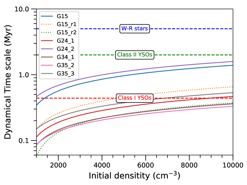
Figure 15.— Variation of the dynamical ages of the ionized gas seen in all selected regions for a range of initial ambient densities. The regions shown in the legend are labeled in Figures 11b and 12. The mean lifetimes of Class I and Class II YSOs, and the typical age of a W–R star are also marked.

Given any initial ambient density, the H ii regions in G34 and G35 are not capable of initiating the formation of YSOs seen in these regions. The ionized gas in the G15 and G24 (G24_r2) are characterized by a dynamical timescale that is sufficiently long to trigger the formation of Class I YSOs in its vicinity. A sequence of Class I YSOs and C¹⁸O condensations can indeed be noted around the ionized gas in the G24 region (see Figure 12a). Such a sequence is a typical signature of triggered star formation by the expansion of the ionized gas. However, no such sequence is seen in any other regions. Note that although VGPS maps typically trace extended radio continuum emission compared to NVSS maps, the VGPS is generally unable to resolve the detailed distribution of the ionized gas because of its lower resolution. Figure 11b shows that the NVSS has resolved two peaks of ionized gas (G15_r1 and G15_r2). The dynamical ages of these two ionized regions are not sufficient to initiate the formation of Class II YSOs, and only one is marginally old enough to initiate the formation of Class I YSOs.

As can be seen in Figure 13, the ionized gas is typically distributed around the molecular shells developed by the W–R stars. Clusters of YSOs and dense condensations are also seen a few pc from the W–R stars (see Figures 11 and 12), but none are generally coincident with the positions of the W-R stars. This observational picture might be explained considering that all W–R stars in our sample have developed expanding molecular shells and created cavities within these shells. Thus, these cavities have lower gas densities, perhaps too low to form any YSOs or cold dust/molecular condensations. In fact, no recent star formation is found within a few pc of our sample W–R stars (see Figures 11b and 12), while clumps and YSO clusters are generally projected at separations of 2–8 pc from the W–R stars. The ionized regions, as well as all identified YSOs, are comparatively younger than the W–R stars, and they are commonly distributed around the molecular shells.

It is also important to note that with typical expansion velocities of 2–5 km s^-1, W–R stars can create shells of 3–8 pc in size within 2 Myr and accumulate matter around the shells, as seen in all our selected regions. In fact, these shells are denser compared to the inner cavities, and the column densities in these molecular shells are enhanced by a minimum of 14$\pm$10% (for the G35 region) to as much as 88$\pm$10% (for the G15 region) compared to the column densities in the cavities (see Table 3). In addition, the surrounding H ii regions have dynamical timescales $\lesssim$2 Myr, even for an initial ambient density of 10,000 cm^-3, which is much younger than the ages of the W–R stars. Higher values of $P_{\mathrm{wind}}$ exerted on the shells than $P_{\mathrm{HII}}$ from the ionized gas (see Table 3) indicate a possibility of further expansion of the shells. All these results indicate that these W–R stars may indeed be responsible for halting recent star formation in their surrounding cavities. An enhanced column density and the presence of active star formation around expanding shells also indicate that molecular gas was collected around these shells which subsequently collapsed to form stars (i.e. the ‘collect and collapse’ scenario). The presence of ionized gas around the shells may trigger further star formation, as seen in the G24 region. Such star formation around W–R shells was already noted by Liu et al. (2012).

M17 is regarded one of the most active Galactic star-forming regions, with a star-formation rate of $\geq 0.004~{}M_{\odot}$ yr^-1 (see Povich et al., 2016, and references therein), which is four times higher than that of the Orion Nebula Cluster. The reason for such a high star-formation rate is still open to debate. Jiang et al. (2002) derived an upper age limit of 3 Myr for M17 which is about 2 Myr younger than the W–R star (typical age of $\sim$5 Myr). The expanding shell with $v_{\mathrm{exp}}$ of 4 km s^-1 driven by the W–R star may reach $\sim$8 pc even in 2 Myr, i.e. the projected separation of the M17 cluster from the W–R star. It is thus possible that the presence of an external driving source, like a W–R star, has caused such a high star-formation rate in M17. Thus, the influence of the W–R star on the M17 region in the context of rapid star formation should be investigated in greater detail.

Overall, the presence of a W–R star significantly affects the dynamics of the parent cloud. The expanding molecular shell driven by a strong stellar wind may create gas-deficient cavities and, thus, further star formation is quenched in those cavities. However, the expanding molecular shell may still help to accumulate molecular gas in the outer layer of the shell, which may collapse and result in further star formation. The impacts of W–R stars might be found in several other Galactic star-forming regions. It is possible that several such regions are still unexplored because of poorly known spectral types and distances of W–R stars. Statistics on the influence of W–R stars on Galactic star formation can be improved if good estimates of the spectral types and better distance calibrations are available for Galactic W–R stars.

7. Conclusions

The primary goal of this study was to explore the impact of W–R stars on their parent molecular clouds. The main results of this study are the following.

1. Strong stellar winds from the W–R stars have created gas-deficient cavities in the host molecular clouds. A signature of these cavities in the parent molecular cloud is found in the form of a trough between the two emission peaks in the ¹³CO spectrum along W–R stars. All the W–R stars in our sample are located at the velocities of the troughs.

2. In all but one region, we identified expanding molecular shells from the $p-v$ analysis of the ¹³CO data. These molecular shells are expanding with velocities of 2–5 km s^-1, and W–R stars are identified as the primary driving sources of this expansion. Although a W–R star is associated with the molecular cloud toward the G34 region, no signature of expanding molecular gas is noted. This is possibly because the red-shifted part of the cloud is significant and sufficiently intense to drown out any ring- or U-like structure in the $p-v$ diagrams.

3. The dynamical ages of none of the H ii regions are sufficiently old to trigger the formation of Class II YSOs seen in our selected regions. However, ionized gas in the G24 region is found to be capable of triggering the formation of Class I YSOs. In fact, a sequence of a cluster of YSOs and molecular condensations is seen around the ionized gas toward the G24 region, indicating recent star formation, possibly triggered by expansion of the ionized gas.

4. Estimation of pressure components reveals that the pressure owing to stellar winds dominates over the radiation pressure of W–R stars by an order of magnitude, and the wind pressure ($P_{\mathrm{wind}}$) is capable of driving the surrounding molecular gas up to a distance of about 10 pc.

5. The M17 region (located toward the G15 region) is a Galactic star-forming region with a high star-formation rate. The expanding shell with $v_{\mathrm{exp}}$ of 4 km s^-1 driven by the W–R star may reach M17 in about 2 Myr. Thus, energetic input from a W–R star within 10 pc could possibly explain the high star-formation rate of the M17 region. The influence of this W–R star on the M17 cluster should be investigated in greater detail.

6. Gas deficient cavities of 2–6 pc in size are identified in molecular column density maps. An absence of recent star formation in all these cavities indicates that stellar winds from W–R stars have dispersed the molecular material from their immediate vicinity and developed these cavities. Star formation is quenched in the cavities.

7. The column densities in cavities generally have lower values and are enhanced by a minimum of 14$\pm$10% (in the G35 region) to as much as 88$\pm$10% (in the G15 region) compared to the surrounding shells. Molecular gas is collected around expanding shells and enhanced column densities. Clusters of YSOs (i.e. Class I–II), massive condensations of 10²–10${}^{3}M_{\odot}$ and ionized gas are typically distributed around these shells. Star formation around the molecular shells might be affected by the W–R stars. Accumulation of molecular gas due to the expansion of the shells could have a positive impact on the recent star formation around the shells.

Overall, it is evident that the stellar winds from W–R stars have a large impact on the dynamics of their surrounding clouds. They are capable of developing gas-deficient cavities surrounded by expanding molecular shells. Although star formation is quenched in those cavities because of the impact of the W–R stars, they may also initiate further star formation in the outer layers of the molecular shells. Several other Galactic regions associated with W–R stars might be explored in greater detail to understand the influence of W–R stars on their parent molecular clouds. Such studies, however, require precise distance estimates to Galactic W–R stars.

Appendix A A. Cloud structures toward field regions

It is not necessary that the double-peaked structures seen in ¹³CO spectra with a trough between the peaks could only develop owing to the presence of W–R stars. In fact, such structures simply signify the presence of two intense parts of the molecular cloud along the sight lines. Similar structures could appear for several reasons. For example, molecular spectra in regions affected by active cloud–cloud collisions also exhibit similar structures (Baug et al., 2016). However, the occurrence of different mechanisms results in distinct signatures in the $p-v$ diagrams. Hence, as a quality control, we constructed molecular spectra along five randomly distributed lines of sight within the field for every region. The corresponding spectra along with the spectrum toward the W-R star for the whole velocity range of the GRS are presented in Figure 16. The spectra for field directions were constructed by summing up all the emission within a 1^′ diameter. We considered slightly larger diameter than the GRS beam (45^′′) to accumulate more emission. The sky coordinates for all spectra are also indicated in the figure. The host molecular clouds studied in this paper are marked with bold lines in Figure 16.

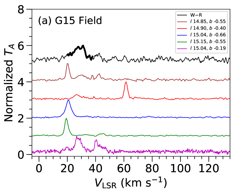
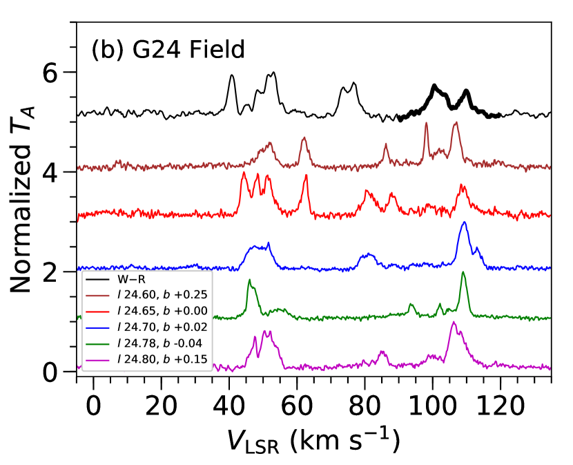
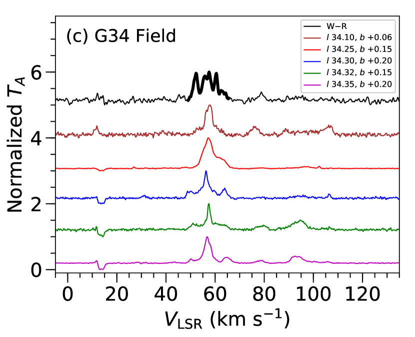
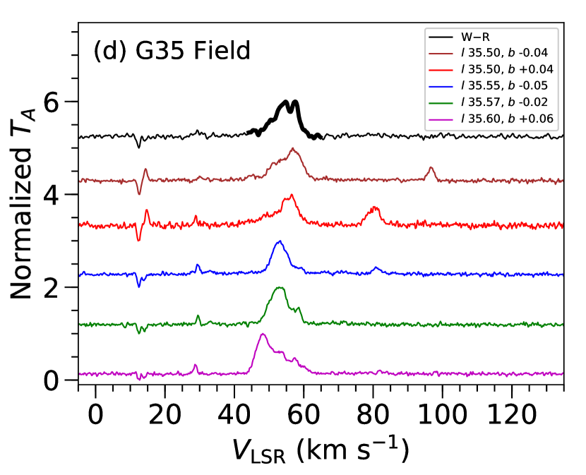
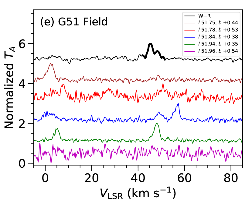
Figure 16.— ¹³CO spectra of five randomly chosen lines of sight for each region: (a) G15, (b) G24, (c) G34, (d) G35, and (e) G51. The spectra were constructed following the same procedure as that applied to the W–R stars, and plotted for the full velocity range of GRS from $-$5–135 km s^-1. The parts of the clouds explored in this paper are marked by bold lines. A few velocity regimes (particularly in the G24 region) show double or multiple peaks for which $p-v$ diagrams are examined.

Double-peaked structures are seen along multiple lines of sight toward the G24 region, and also toward the G15 and G51 regions. Another cloud with double-peaked emission features ($v_{\mathrm{LSR}}~{}\sim$ 70–82 km s^-1) is also seen in the ¹³CO spectrum along the W–R star in the G24 region. Thus, to understand the origin of these double- or triple-peaked structures, we constructed $p-v$ diagrams of these particular clouds. The corresponding $p-v$ diagrams are presented in Figures 17, 18, and 19. The $p-v$ diagrams of all but one sight line (in G24 field) indicate the presence of two distinct molecular clouds, but no signature of expanding molecular gas is seen along these lines of sight including the cloud at $v_{\mathrm{LSR}}~{}\sim$ 70–82 km s^-1 toward the W–R star in the G24 region (see Figures 19d,e,f). One cloud toward the G24 field shows a ring-like structure in the $p-v$ diagram (see Figure 18b) that resembles the expansion of molecular gas. Therefore, we explored the possible driver of the expanding gas, and found an YSO candidate reported by Robitaille et al. (2008). We also modeled the spectral energy distribution (SED) of the source using the SED fitting tool of Robitaille et al. (2006) which results the source to be a Class I YSO with a mass of 5.0$\pm$0.5 M_⊙ and a surface temperature of 14,000$\pm$2200 K. This particular source is hot and massive enough to drive expansion of the surrounding molecular gas. All these results eventually signify that the ring-like structures in the $p-v$ diagrams seen around W–R stars are signatures of expanding molecular gas driven by the strong energetics from W–R stars.

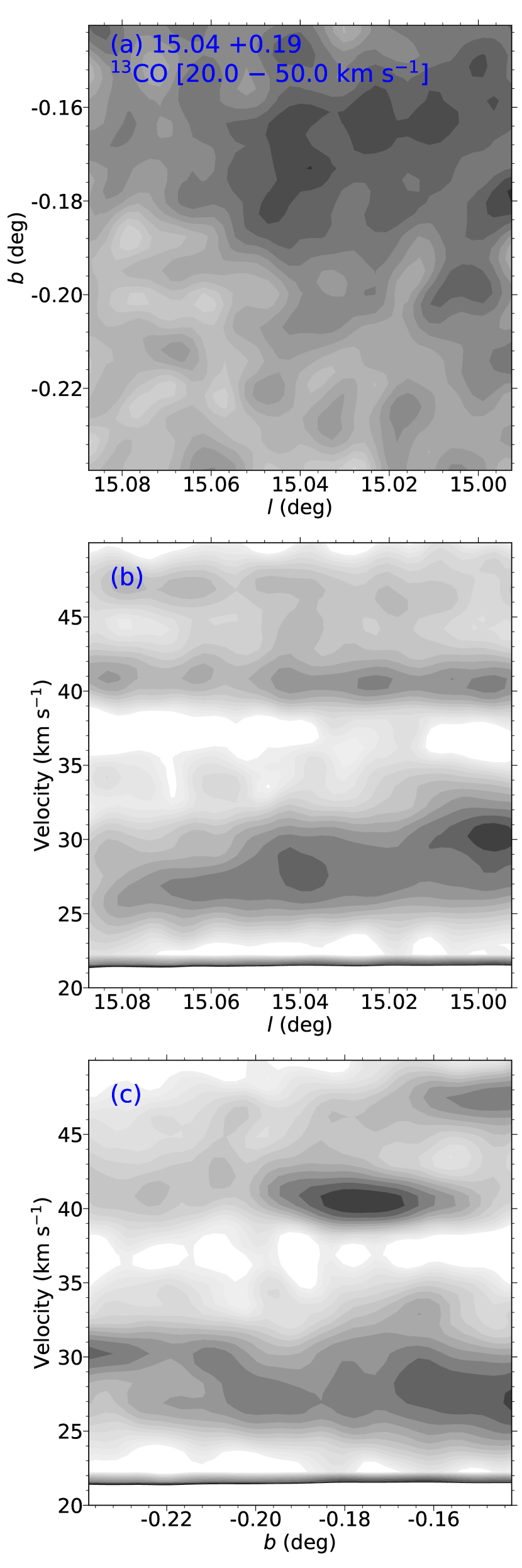
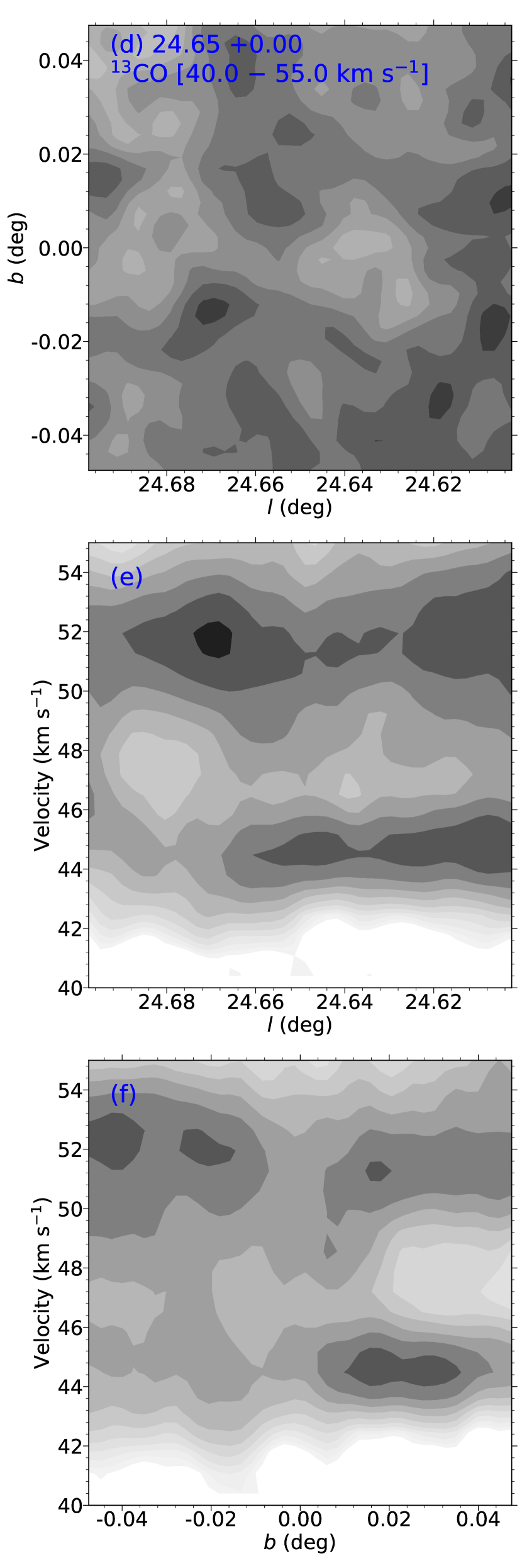
Figure 17.— (a) and (d) Integrated intensity map of the field regions (labeled in each figure) for the respective velocity range (marked) where multiple peaks are seen in the ¹³CO spectrum (in Figure 16). (b), (c), (e) and (f) Corresponding $p-v$ diagrams.

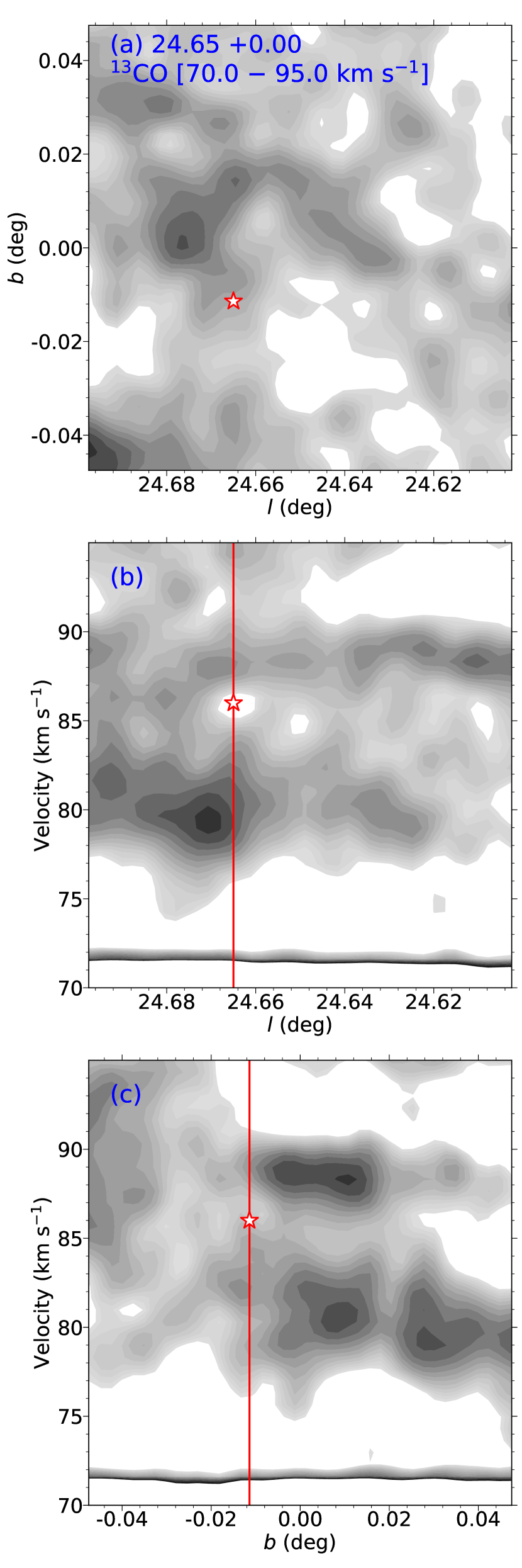
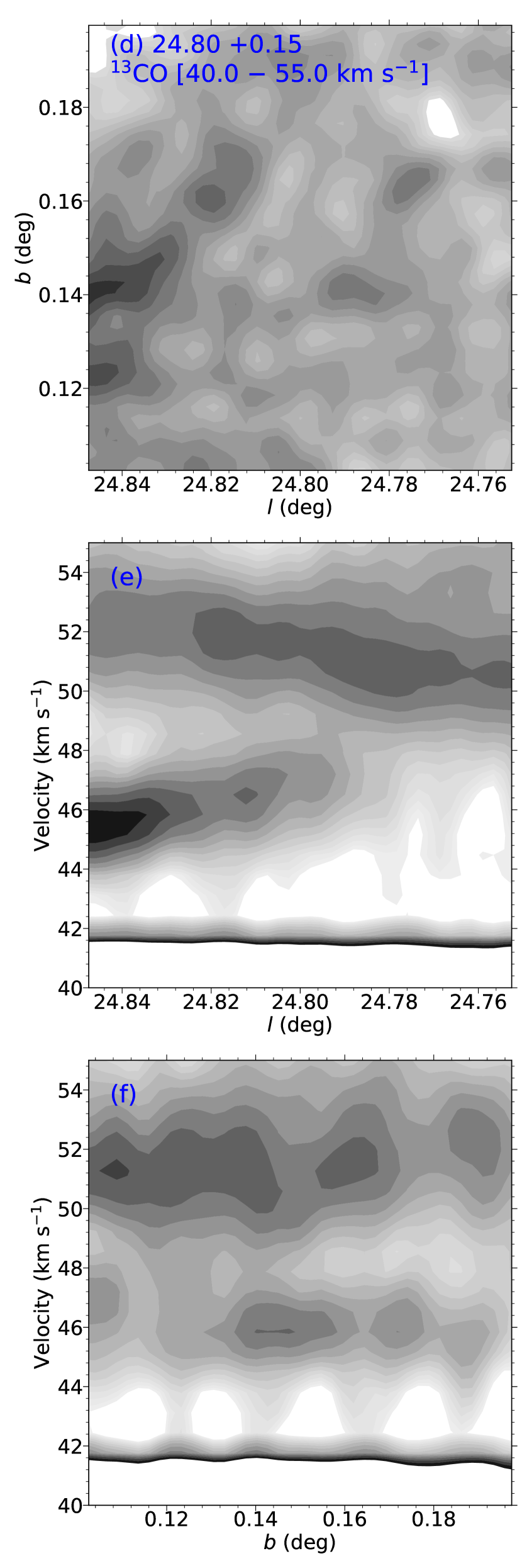
Figure 18.— As Figure 17. In these $p-v$ diagrams, ring-like structures are easily discerned. A ring-like structure can be seen in (b). The possible source (an intermediate mass YSO) of these ring-like structures (or expansion) is marked by a star.

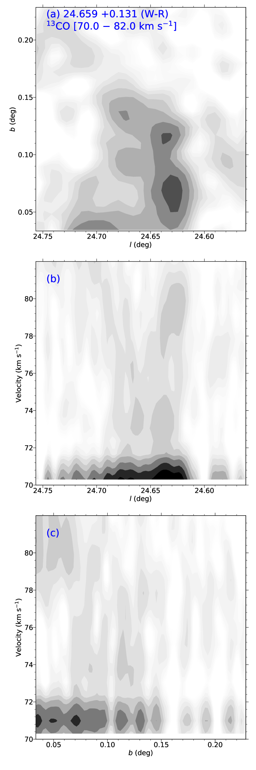
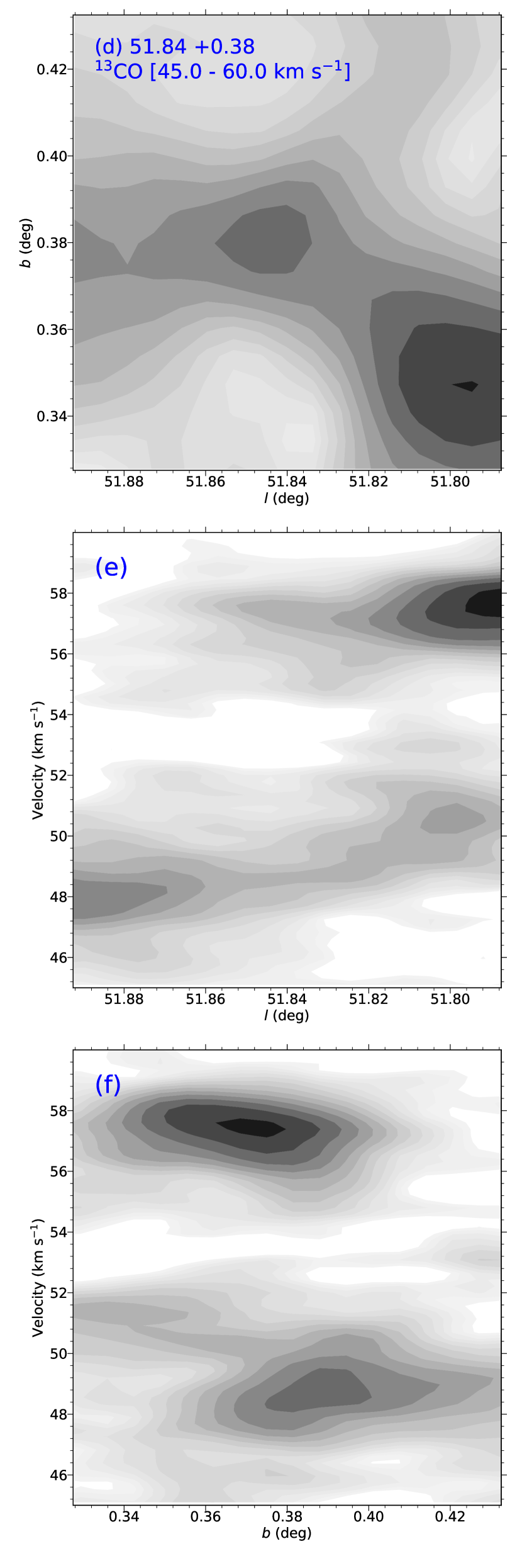
Figure 19.— As Figure 17. No ring-like structure is seen in these $p-v$ diagrams.

References

- Arce et al. (2011) Arce, H. G., Borkin, M. A., Goodman, A. A., Pineda, J. E., & Beaumont, C. N. 2011, ApJ, 742, 105
- Anderson et al. (2009) Anderson, L. D., & Bania, T. M. 2009, ApJ, 690, 706
- Anderson et al. (2011) Anderson, L. D., Bania, T. M., Balser, D. S., et al. 2011, ApJS, 194, 32
- Anderson et al. (2012) Anderson, L. D., Bania, T. M., Balser, D. S., & Rood, R. T. 2012, ApJ, 754, 62
- Bailer-Jones et al. (2018) Bailer-Jones, C. A. L., Rybizki, J., Fouesneau, M., Mantelet, G., & Andrae, R. 2018, AJ, 156, 58
- Bania et al. (2010) Bania, T. M., Anderson, L. D., Balser, D. S., & Rood, R. T. 2010, ApJ, 718, L106
- Bania et al. (2012) Bania, T. M., Anderson, L. D., & Balser, D. S. 2012, ApJ, 759, 96
- Baug et al. (2015) Baug, T., Ojha, D. K., Dewangan, L. K., et al. 2015, MNRAS, 454, 4335
- Baug et al. (2016) Baug, T., Dewangan, L. K., Ojha, D. K., & Ninan, J. P. 2016, ApJ, 833, 85
- Baug et al. (2018) Baug, T., Dewangan, L. K., Ojha, D. K., et al. 2018, ApJ, 852, 119
- Benjamin et al. (2003) Benjamin, R. A., Churchwell, E., Babler, B. L., et al. 2003, PASP, 115, 953
- Bertoldi (1989) Bertoldi, F. 1989, ApJ, 346, 735
- Bisbas et al. (2009) Bisbas, T. G., Wünsch, R., Whitworth, A. P., & Hubber, D. A. 2009, A&A, 497, 649
- Carey et al. (2005) Carey, S. J., Noriega-Crespo, A., Price, S. D., et al. 2005, BAAS, 37, 63.33
- Chibueze et al. (2016) Chibueze, J. O., Kamezaki, T., Omodaka, T., et al. 2016, MNRAS, 460, 1839
- Churchwell et al. (2006) Churchwell, E., Povich, M. S., Allen, D., et al. 2006, ApJ, 649, 759
- Churchwell et al. (2007) Churchwell, E., Watson, D. F., Povich, M. S., et al. 2007, ApJ, 670, 428
- Cichowolski et al. (2015) Cichowolski, S., Suad, L. A., Pineault, S., et al. 2015, MNRAS, 450, 3458
- Condon et al. (1998) Condon, J. J., Cotton, W. D., Greisen, E. W., et al. 1998, AJ, 115, 1693
- Crowther (2007) Crowther, P. A. 2007, ARA&A, 45, 177
- Crowther et al. (2006) Crowther, P. A., Hadfield, L. J., Clark, J. S., Negueruela, I., & Vacca, W. D. 2006, MNRAS, 372, 1407
- Cutri et al. (2003) Cutri, R. M., Skrutskie, M. F., van Dyk, S., et al. 2003, The 2MASS All Sky Catalog of Point Sources (available at https://www.ipac.caltech.edu/2mass/)
- Dale et al. (2013) Dale, J. E., Ngoumou, J., Ercolano, B., & Bonnell, I. A. 2013, MNRAS, 436, 3430
- Deharveng et al. (2008) Deharveng, L., Lefloch, B., Kurtz, S., et al. 2008, A&A, 482, 585
- Deharveng et al. (2010) Deharveng, L., Schuller, F., Anderson, L. D., et al. 2010, A&A, 523, A6
- Devine et al. (2018) Devine, K., Mori, J., Watson, C., Trujillo, L., & Hicks, M. 2018, ApJ, 861, 117
- Dewangan et al. (2016) Dewangan, L. K., Baug, T., Ojha, D. K., et al. 2016, ApJ, 826, 27
- Dewangan et al. (2018) Dewangan, L. K., Dhanya, J. S., Ojha, D. K., & Zinchenko, I. 2018, ApJ, 866, 20
- Dyson & Williams (1980) Dyson, J. E., & Williams, D. A. 1980, New York, Halsted Press, 1980. 204 p.,
- Elmegreen (1998) Elmegreen, B. G. 1998, Origins, 148, 150
- Elmegreen & Lada (1977) Elmegreen, B. G., & Lada, C. J. 1977, ApJ, 214, 725
- Evans et al. (2009) Evans, N. J., II, Dunham, M. M., Jrgensen, J. K., et al. 2009, ApJS, 181, 321
- Faúndez et al. (2004) Faúndez, S., Bronfman, L., Garay, G., et al. 2004, A&A, 426, 97
- Feddersen et al. (2018) Feddersen, J. R., Arce, H. G., Kong, S., et al. 2018, ApJ, 862, 121
- Fontani et al. (2012) Fontani, F., Caselli, P., Zhang, Q., et al. 2012, A&A, 541, A32
- Foster et al. (2012) Foster, J. B., Stead, J. J., Benjamin, R. A., Hoare, M. G., & Jackson, J. M. 2012, ApJ, 751, 157
- Gaia Collaboration et al. (2018) Gaia Collaboration, Brown, A. G. A., Vallenari, A., et al. 2018, A&A, 616, A1
- Griffin et al. (2010) Griffin, M. J., Abergel, A., Abreu, A, et al. 2010, A&A, 518L, 3
- Gutermuth & Heyer (2015) Gutermuth, R. A., & Heyer, M. 2015, AJ, 149, 64
- Hadfield et al. (2007) Hadfield, L. J., van Dyk, S. D., Morris, P. W., et al. 2007, MNRAS, 376, 248
- Jackson et al. (2006) Jackson, J. M., Rathborne, J. M., Shah, R. Y., et al. 2006, ApJS, 163, 145
- Jiang et al. (2002) Jiang, Z., Yao, Y., Yang, J., et al. 2002, ApJ, 577, 245
- Kanarek et al. (2015) Kanarek, G., Shara, M., Faherty, J., Zurek, D., & Moffat, A. 2015, MNRAS, 452, 2858
- Kohno et al. (2018) Kohno, M., Tachihara, K., Fujita, S., et al. 2018, PASJ, arXiv:1809.00118, in press
- Kurtz (2002) Kurtz, S. 2002, in ASP Conf. Ser. 267, Hot Star Workshop III: The Earliest Phases of Massive Star Birth, ed. Crowther P. A. (San Francisco, CA: ASP), 81
- Kurayama et al. (2011) Kurayama, T., Nakagawa, A., Sawada-Satoh, S., et al. 2011, PASJ, 63, 513
- Lamers & Cassinelli (1999) Lamers, H. J. G. L. M., & Cassinelli, J. P. 1999, Introduction to Stellar Winds, by H. J. G. L. M. Lamers and J. P. Cassinelli, pp. 452. ISBN 0521593980. Cambridge, UK: Cambridge University Press, June 1999., 452
- Lefloch & Lazareff (1994) Lefloch, B., & Lazareff, B. 1994, A&A, 289, 559
- Li et al. (2013) Li, G.-X., Wyrowski, F., Menten, K., & Belloche, A. 2013, A&A, 559, A34
- Liu et al. (2012) Liu, T., Wu, Y., Zhang, H., & Qin, S.-L. 2012, ApJ, 751, 68
- Mallick et al. (2015) Mallick, K. K., Ojha, D. K., Tamura, M., et al. 2015, MNRAS, 447, 2307
- Marston (1996) Marston, A. P. 1996, AJ, 112, 2828
- Minamidani et al. (2016) Minamidani, T., Nishimura, A., Miyamoto, Y., et al. 2016, Proc. SPIE, 9914, 99141Z
- Moran (1983) Moran, J. M. 1983, Rev. Mexicana Astron. Astrofis., 7, 95
- Morgan et al. (2010) Morgan, L. K., Figura, C. C., Urquhart, J. S., & Thompson, M. A. 2010, MNRAS, 408, 157
- Motte et al. (2018) Motte, F., Bontemps, S., & Louvet, F. 2018, ARA&A, 56, 41
- Nugis & Lamers (2000) Nugis, T., & Lamers, H. J. G. L. M. 2000, A&A, 360, 227
- Ogura et al. (2007) Ogura, K., Chauhan, N., Pandey, A. K., et al. 2007, PASJ, 59, 199
- Panagia (1973) Panagia, N. 1973, AJ, 78, 929
- Panwar et al. (2014) Panwar, N., Chen, W. P., Pandey, A. K., et al. 2014, MNRAS, 443, 1614
- Poglitsch et al. (2010) Poglitsch, A., Waelkens, C., Geis, N., et al. 2010, A&A, 518, L2
- Pomarès et al. (2009) Pomarès, M., Zavagno, A., Deharveng, L., et al. 2009, A&A, 494, 987
- Povich et al. (2016) Povich, M. S., Townsley, L. K., Robitaille, T. P., et al. 2016, ApJ, 825, 125
- Rathborne et al. (2006) Rathborne, J. M., Jackson, J. M., & Simon, R. 2006, ApJ, 641, 389
- Reid et al. (2014) Reid, M. J., Menten, K. M., Brunthaler, A., et al. 2014, ApJ, 783, 130
- Reipurth (1983) Reipurth, B. 1983, A&A, 117, 183
- Robitaille et al. (2008) Robitaille, T. P., Meade, M. R., Babler, B. L., et al. 2008, AJ, 136, 2413
- Robitaille et al. (2006) Robitaille, T. P., Whitney, B. A., Indebetouw, R., et al. 2006, ApJS, 167, 256
- Rosolowsky et al. (2008) Rosolowsky, E. W., Pineda, J. E., Kauffmann, J., & Goodman, A. A. 2008, ApJ, 679, 1338
- Sakai et al. (2018) Sakai, T., Yanagida, T., Furuya, K., et al. 2018, ApJ, 857, 35
- Schmeja et al. (2008) Schmeja, S., Kumar, M. S. N., & Ferreira, B. 2008, MNRAS, 389, 1209
- Shara et al. (2012) Shara, M. M., Faherty, J. K., Zurek, D., et al. 2012, AJ, 143, 149
- Simon et al. (2006) Simon, R., Rathborne, J. M., Shah, R. Y., Jackson, J. M., & Chambers, E. T. 2006, ApJ, 653, 1325
- Simpson et al. (2012) Simpson, R. J., Povich, M. S., Kendrew, S., et al. 2012, MNRAS, 424, 2442
- Skrutskie et al. (2006) Skrutskie, M. F., Cutri, R. M., Stiening, R., et al. 2006, AJ, 131, 1163
- Sokal et al. (2016) Sokal, K. R., Johnson, K. E., Indebetouw, R., & Massey, P. 2016, ApJ, 826, 194
- Stil et al. (2006) Stil, J. M., Taylor, A. R., Dickey, J. M., et al. 2006, AJ, 132, 1158
- Torii et al. (2019) Torii, K., Fujita, S., Nishimura, A., et al. 2019, PASJ, arXiv:1809.06642, in press
- Umemoto et al. (2017) Umemoto, T., Minamidani, T., Kuno, N., et al. 2017, PASJ, 69, 78
- Urquhart et al. (2018) Urquhart, J. S., König, C., Giannetti, A., et al. 2018, MNRAS, 473, 1059
- Urquhart et al. (2007) Urquhart, J. S., Thompson, M. A., Morgan, L. K., et al. 2007, A&A, 467, 1125
- van der Hucht (2001) van der Hucht, K. A. 2001, New A Rev., 45, 135
- van der Hucht (2006) van der Hucht, K. A. 2006, A&A, 458, 453
- Wang et al. (2016) Wang, K., Testi, L., Burkert, A., et al. 2016, ApJS, 226, 9
- Watson et al. (2003) Watson, C., Araya, E., Sewilo, M., et al. 2003, ApJ, 587, 714
- Wenger et al. (2018) Wenger, T. V., Balser, D. S., Anderson, L. D., & Bania, T. M. 2018, ApJ, 856, 52
- Whitworth et al. (1994) Whitworth, A. P., Bhattal, A. S., Chapman, S. J., Disney, M. J., & Turner, J. A. 1994, MNRAS, 268, 291
- Williams et al. (1994) Williams, J. P., de Geus, E. J., & Blitz, L. 1994, ApJ, 428, 693
- Wu et al. (2014) Wu, Y. W., Sato, M., Reid, M. J., et al. 2014, A&A, 566, A17
- Xu et al. (2016) Xu, J.-L., Li, D., Zhang, C.-P., et al. 2016, ApJ, 819, 117
- Zavagno et al. (2007) Zavagno, A., Pomarès, M., Deharveng, L., et al. 2007, A&A, 472, 835
- Zavagno et al. (2010a) Zavagno, A., Anderson, L. D., Russeil, D., et al. 2010, A&A, 518, L101
- Zavagno et al. (2010b) Zavagno, A., Russeil, D., Motte, F., et al. 2010, A&A, 518, L81
- Zhang & Wang (2013) Zhang, C.-P., & Wang, J.-J. 2013, RAA, 13, 47