Isotope shifts in ^20,22Ne - Precision measurements and global analysis in the framework of intermediate coupling

Abstract

We report new precision measurements of the ²⁰Ne–²²Ne isotope shift for several transitions, as well as state-of-the-art, ab initio field-shift calculations. Our results are combined with historical measurements in a global fit to obtain the isotope shifts of all fifty low-lying neon levels with high precision. These level shifts show a wealth of electronic, nuclear, and relativistic phenomena. Relying on the analogy between mass shift and fine-structure operators, we explain this plethora of neon level-shifts utilizing a small number of effective parameters in a global parametric investigation. This investigation provides a birds-eye view on the isotope shift phenomena in noble gasses. From this vantage point, we reinterpret every effort made to calculate neon mass-shifts ab initio, and show that a remarkable agreement between experiment and theory is obtained.

I Introduction

Upon analyzing the mass spectrum of neon ions emerging from canal rays, J. J. Thompson and W. Wein observed a weak line at $22$ atomic mass units Thomson (1912). This observation led to the discovery that a specific element may be found with different mass, an isotope. Soon after, T. R. Merton suggested the possibility of detection of neon isotopes by spectroscopic means Thomson et al. (1921), owing to small lineshifts between them generally referred to as isotope shifts (IS).

Isotope shifts are minute differences between the electronic energy levels of different isotopes of the same element. Today they are the focus of a multitude of theoretical and experimental efforts due to their importance for atomic and nuclear physics. For few electron-systems such as hydrogen Huber et al. (1998); Jentschura et al. (2011), helium Monkhorst (1994); Pachucki and Yerokhin (2015); Pachucki et al. (2017), lithium Yan and Drake (2000); Nörtershäuser et al. (2011), and ions such as Ar¹³⁺ Draganić et al. (2003); Orts et al. (2006), accurate theory is available and so very precise measurements determine parameters such as charge radii Lu et al. (2013), as well as test bound-state QED Nörtershäuser et al. (2015). The theory for isotope shifts of multielectron atoms is more involved; nevertheless, their IS are of interest for astrophysical searches for $\alpha$-variation Ashenfelter et al. (2004); Korol and Kozlov (2007); Berengut et al. (2011), probing for atomic Higgs and new Higgs-Like forces Delaunay et al. (2017), as well as other new-physics scenarios Frugiuele et al. (2017).

From a nuclear physics perspective, isotope shifts combine different precise atomic physics probes for studying nuclear properties, and their main use is nuclear-model-independent determination of (RMS) charge-radii differences Brix and Kopfermann (1958); Otten (1989); Palffy (2010); Campbell et al. (2016). The shape of some light isotopes ($A<30$) vary wildly from the liquid-drop model Campbell et al. (2016); Freer et al. (2018), and display exotic phenomena such as proton and neutron halos Tanihata (1996); Wang et al. (2004); Sanchez et al. (2006); Mueller et al. (2007); Nörtershäuser et al. (2009). On the other hand, the nuclear shape effect on the isotope shifts of light atoms is small compared with the total IS. Thus, for the determination of radii differences for light multielectron isotopes, both experiment and theory must display high precision and accuracy.

The isotope shifts of neon constitute a compelling case, and are the focus of this work. From the experimental perspective, a great multitude of lineshifts in the ^20,22Ne pair has been measured over the last hundred years (see references in tables 8, and 9), and including this work, some very precise results exist for a number of lines. From a theoretical perspective, even-even neon isotopes, which do not possess a hyperfine structure, provide a clean environment to investigate the IS phenomena in light atomic systems with strong electron-hole interactions.

When analyzed globally, the plethora of experimental information gathered here not only gives an improved precision and accuracy in IS determination, but enables benchmarking and cross-checking theoretical calculations from a birds-eye perspective. We show that alleged large discrepancies between experiment and theory, which dominated theoretical work on neon isotope shifts in the last hundred years, are removed upon a reanalysis and reinterpretation enabled by our investigation.

The remainder of this paper is organized as follows. In Sec. II we provide a short background on the origins of the isotope shift phenomena and introduce the notations to be used in the following sections.

Sec. III presents new, ab initio, field shift calculations, covering all relevant neon configurations. An immediate application of this calculation is a considerable update to the RMS charge radii differences of stable and unstable neon isotopes, and their uncertainty. The updated field shifts are used in the following sections for comparison between experiment and theory, since they were not taken into account in most calculations.

In Sec. IV we present precision measurements of the ^20,22Ne isotope shifts for several transitions between the $2p^{5}3s$ and $2p^{5}3p$ manifolds. The small experimental uncertainty results from the use of the new measurement scheme of Dual-sideband Saturated absorption Spectroscopy Ohayon et al. (2017). In Sec. V, our measurements, as well as every other relevant isotope shift measurement existing in the literature, are averaged line by line, accounting for outliers and inconsistencies.

In Sec. VI, we extract the residual-shifts of levels from a global linear fit to the average lineshifts. The lineshifts are then recalculated from levels resulting in a large increase in precision. The calculated lineshifts are presented in tables 8 and 9 and do not depend on any atomic physics theoretical framework.

In order to interpret, as well as significantly reduce the uncertainty in the level shifts we utilize the strong analogy between specific mass shifts (SMS) and fine-structure operators. First, in Sec. VII, we investigate the fine-structure of neon in the framework of intermediate coupling to obtain an approximate expansion of the relevant wavefunctions over LS and jj-coupled bases. Utilizing the angular coefficients of this expansion, we introduce in Sec. VIII, a small set of effective parameters for each configuration, with the same angular coefficients. These intraconfiguration parameters identify and differentiate between relativistic, 1, and 2-order SMS effects, and are extracted from fitting the average lineshifts of Sec. V directly. Recalculating the level shifts from a smaller number of IS parameters dramatically reduces the uncertainty and so reveals the structure of poorly measured configurations.

In Sec. IX, a smaller set of effective IS parameters is used in a similar way, relying on a deeper analogy between fine-structure and SMS effects. Thus a phenomenological understanding as to the origin of various SMS effects is gained, and a greater precision in the levelshifts is obtained.

In Sec. X, we review all previous efforts for calculating neon isotope shifts ab initio. Each theoretical effort is examined and reinterpreted in light of the phenomenological parameters of Sec VIII and IX, as well as the field shifts of Sec. III.

Section XI is devoted to conclusions and outlook.

II Origins of the isotope shift

Isotope shifts result from a change in the mass and the charge distribution of the nucleus, which corresponds to a mass shift (MS), which predominates in light elements; and field shift (FS), which is the main effect in heavy atoms. For a multi-electron-system, and in the non-relativistic limit, the mass shift is composed of a normal mass shift (NMS), resulting from a change in the reduced mass of the electron, and a specific mass shift (SMS), which is sensitive to electron correlations Hughes and Eckart (1930).

Denoting the heavier isotope by $H$ and the lighter by $L$, the isotope shift of a transition with frequency $\nu$ is

$$\delta\nu^{\mathrm{L,H}}=\nu_{\mathrm{H}}-\nu_{\mathrm{L}}$$ (1)

and the NMS in the non-relativistic limit is defined as King (2013):

$$\delta\nu^{\mathrm{L,H}}_{\mathrm{NMS}}=\nu_{\mathrm{L}}m\frac{M_{\mathrm{H}}-M_{\mathrm{L}}}{M_{\mathrm{L}}(M_{\mathrm{H}}+m)},$$ (2)

where $m$ is the electron mass, and we adopt the convention that an isotope shift is positive when the line of the heavier isotope corresponds to the higher frequency.

The NMS as defined by (2) is the main contribution to the IS of light atoms King (2013), and amounts to approximately $1$ GHz in the optical lines of neon; however, owing to precise neon mass measurements Geithner et al. (2008a), one may subtract it without introducing appreciable contributions to the uncertainty. The largest relevant NMS uncertainty is in the most energetic lines ($63$ nm) and amounts to only a few kHz resulting from uncertainty in the wavelength Saloman and Sansonetti (2004).

As early as 1930, Nagaoka and Mishima Nagaoka (1930) observed a strong deviation from the NMS formula for neon lines, indicating there are other important effects. After subtracting the NMS, the remaining shift is denoted the residual isotope shift (RIS) Bauche and Champeau (1976). It includes the SMS, the FS, and relativistic corrections to all effects, which are non-negligible in the level of precision presented here.

The SMS depends on correlations between electrons and its calculation is very sensitive to the details of the wavefunctions used King (2013). In light elements ($Z<30$), it is by far the strongest contribution to the RIS for transitions and can be either positive or negative depending on the nature of correlations Bauche and Champeau (1976). It can be reliably calculated with very high precision only in very light elements with few electrons, five electrons being the forefront of such calculations Puchalski et al. (2015); Maaß et al. (2019).

The FS in neon can only be observed with high precision, and so until the turn of the century have been considered negligible Geithner et al. (2000). Since it is small, a 1-order picture is adopted here, where the change in energy of a level is proportional to the change in total electron probability density at the origin, times the mean-square charge radius difference $\delta\langle r^{2}\rangle$ Rosenthal and Breit (1932):

$$\delta\nu_{\mathrm{FS}}=F\times\delta\langle r^{2}\rangle,$$ (3)

where $F$ the so called field-shift factor (FSF) of the level. Under the above convention, for transitions where the upper level has a lower electron density at the origin than the lower level, then the FSF is negative Nazé (2012).

III Field-Shift factors and neon charge radii

Table 1: Calculated field-shift factors of neon levels relative to the ground state, in MHz/fm². Uncertainties are estimated from the rate of convergence (parenthesis), and are dominated by uncertainty in the FS-factor of the ground state (square brackets). The last line is the field shift of the $614$ nm transition. Comparison with previous calculations is presented where available. The last column gives the field shift obtained from eq. 3 utilizing radii measurements, with correlated uncertainty in square brackets dominated by nuclear model.

	This Work	Li et al. (2016)	Nazé (2012)	Geithner et al. (2000)	FS (MHz)
Method:	CI+MBPT	MCDHF	MCDHF	GFS
$3s$	142(2)[6]	138	139		-44[5]
$3p$	112(1)[6]				-35[4]
$4s$	118(1)[6]				-37[4]
$3d$	114(1)[6]				-35[4]
$4p$	111(2)[6]				-35[4]
$5s$	115(2)[6]				-36[4]
$4d$	112(1)[6]				-35[4]
$4f$	112(1)[6]				-35[4]
$3s[3/2]_{2}$
$\rightarrow 3p[3/2]_{2}$	-30.5(1.1)	-32.3		-40(4)	9.5[1.0]

Whereas SMS effects are considered difficult to calculate ab initio with high precision, calculations of the FSF of Eq. 3 have reached the point where they are considered trustworthy in a multitude of scenarios, with uncertainties on the order of a few percent Marinova (2015); Campbell et al. (2016).

We performed relativistic ab initio field shift calculations in neon using the AMBiT software Kahl and Berengut (2019). AMBiT calculates the electronic structure of a given atom using a combination of particle-hole configuration interaction (CI) and many-body perturbation theory (MBPT); this has been thoroughly detailed in Kahl and Berengut (2019); Berengut (2016). The orbitals in a CI+MBPT calculation are divided into valence and core orbitals. The valence-valence correlations are treated with CI while MBPT is applied to the core-valence interactions Dzuba et al. (1996).

Our calculations in neon begin with a Dirac-Hartree-Fock (DHF) calculation. Each electron is treated as a single electron in a mean field $V^{N_{\mathrm{DF}}}$ arising from all electrons $N_{\mathrm{DF}}$ included in the DHF method. We selected a $V^{N-1}$ potential, which corresponds to the average potential from all but one of the electrons in neon. A single electron basis set is then constructed from B-splines in the DHF potential, these are used for the valence and virtual orbitals Shabaev et al. (2004); Johnson et al. (1988).

The emu CI method, which is explained in detail in Geddes et al. (2018), is used instead of conventional CI in order to decrease computational time and improve convergence. We construct our configuration state functions (CSFs) by single or double excitation of electrons and holes from the leading configurations $0$ (i.e. the closed-shell configuration $1s^{2}\ 2s^{2}\ 2p^{6}$), $2p^{-1}3s^{1}$, $2p^{-1}3p^{1}$ and $2p^{-1}3d^{1}$. The ’$-1$’ superscript in the aforementioned configurations represents a hole state in a given orbital relative to the closed-shell configuration. In neon, we restrict our single particle basis set to $13spdf$ for the CI calculation (that is, we only include excitations to valence and virtual orbitals up to $n=13$ and $l=3$). We also allow hole excitations to the $2s$ and $2p$ core shells, while correlations with the $1s$ orbital are included using MBPT. Our use of emu CI ignores correlations between high-energy doubly-excited states. The MBPT method introduced in Dzuba et al. (1996) has been implemented in AMBiT using the diagrammatical technique described in Berengut et al. (2006). The neon calculation included one, two and three body core-valence diagrams at the second order of perturbation theory using a virtual basis set of $30spdfg$.

The Coulomb potential in AMBiT includes the effect of a finite nuclear charge distribution with a Fermi-Dirac distribution. Therefore we can use the “finite field” method to obtain field shift coefficients for neon. We modify the root-mean nuclear charge radii $\langle r^{2}\rangle$ in regular increments, performing the entire CI+MBPT calculation each time to obtain transition energies $\omega$. The FSFs are extracted as

$$F=\frac{\delta\omega}{\delta\langle r^{2}\rangle}.$$ (4)

The results of our calculation for the FSF of each configuration, relative to the ground state, are given in table 1. The uncertainty is estimated from the convergence rate with a varying number of basis functions, as well as the ability of the code to recreate the level energies ($4\%)$. It is dominated by the ground state calculation. The FSF variance within each configuration is smaller than our quoted uncertainty, and thus for the current level of precision, we regard each configuration as having the same FSF, nevertheless, for specific transitions, the exact FSF is quoted. For the relative FSF between configurations, i.e. the 614 nm transition of which the IS was measured for unstable isotopes Marinova et al. (2011), the uncertainty is slightly lower, as the ground state is not involved. We note that for non-s states, the FSF quickly converges to the ionization limit, estimated as $112(1)[6]$ MHz/fm².

The few ab initio calculations that are available in the literature Li et al. (2016); Nazé (2012) are tabulated as well, and an agreement is found to the level of a few percent. Note that we reversed the sign of the field shift factor as it appears in Li et al. (2016); when adding two neutrons to ²⁰Ne, the nuclear charge radius shrinks, resulting in a larger binding energy for the valence $2p^{5}3s$ electron and a negligible field change for the $2p^{5}3p$ electron. Thus $s-p$ transitions are more energetic for ²²Ne, resulting in a positive field shift. Assuming that the calculations of Li et al. (2016), which used the Multiconfiguration Dirac-Hartree-Fock method, have a comparable uncertainty, as indicated by his convergence rate, our results are in agreement. Focusing on the $614$ nm transition, we consider a weighted FS-factor value of: $-31.4(0.9)$ MHz/fm². This value is four times as precise as, and disagrees with, the value of $-40(4)$ MHz/fm² estimated by Geithner et al. (2000) utilizing the semi-empirical GFS formula. It is noteworthy to mention that a $25\%$ disagreement between ab initio and semi-empirical calculations was found in Mg $s-p$ transitions Berengut et al. (2003).

Substituting the FSF of table 1 in Eq. 3, along with the independently measured muonic X-ray measurements of $\delta\langle r^{2}\rangle^{20,22}=-0.31[3]$ Fricke et al. (1995), we obtain the FS for each transition, with a correlated systematic uncertainty dominated by the nuclear model Marinova et al. (2011).

We utilize the $614$ nm transition field shift to update the RMS charge radii differences of ^{17-19,21-26,28}Ne, $\delta\langle r^{2}\rangle^{20,A}$, utilizing the IS results presented in Marinova et al. (2011). Given in table 2, the effect of the updated FS-factor and its reduced uncertainty on $\delta\langle r^{2}\rangle^{20,A}$, is dramatic. Eq. 3 predicts that once a FS is given, there exists a linear relationship between the FS factor and the deduced radii differences; and indeed, the statistical uncertainty is larger by $25\%$; however, the updated values differ substantially from the previous. This difference stems from the fact that the FS-factor is used to calibrate the mass shift in a modified king-plot procedure Marinova et al. (2011). We find a new mass shift factor $363.73(23)$ GHz u with uncertainty dominated by statistics, where the previous one $363.07[43]$ GHz u with uncertainty dominated by that of the FSF.

The updated $\delta\langle r^{2}\rangle^{20,A}$ of table 2 posses a smaller total uncertainty and agree better with the x-ray measurements for stable isotopes Fricke et al. (1995), with the Droplet-model predictions of Marinova et al. (2011), and with recent ab initio coupled cluster calculations Jansen et al. (2016).

On top of updating the RMS charge radii differences, the FSF results presented in this section are utilised in Sec. X for a comparison between analyzed neon isotope shift measurements and revisited mass shift calculations.

Table 2: RMS charge radii difference in fm² with updated field shift factor from this work. Statistical uncertainty resulting from original IS measurements is in parenthesis. Correlated systematic uncertainty in square brackets and affect the general slope around the ²⁰Ne point Marinova (2015).

A	$\delta\langle r^{2}\rangle^{20,A}$ Marinova et al. (2011)	$\delta\langle r^{2}\rangle^{20,A}$ Updated	$r_{\mathrm{ch}}$ (fm)
17	0.220(29) [123]	0.097(37) [092]	3.022(6) [15]
18	-0.207(15) [112]	-0.380(20) [071]	2.942(3) [12]
19	0.017(19) [041]	-0.033(24) [029]	3.001(4) [05]
20	0	0	3.006     [02]
21	-0.217(14) [024]	-0.227(18) [022]	2.968(3) [04]
22	-0.321(04) [043]	-0.314(05) [040]	2.953(1) [07]
23	-0.571(34) [064]	-0.592(44) [059]	2.906(8) [10]
24	-0.627(19) [075]	-0.624(24) [072]	2.900(4) [12]
25	-0.429(16) [122]	-0.336(21) [099]	2.950(4) [17]
26	-0.484(18) [143]	-0.374(22) [114]	2.943(4) [19]
28	-0.239(35) [213]	-0.004(44) [155]	3.005(7) [26]

IV Precision Measurements of neon isotope shifts

We use the method of Dual-sideband Saturated Absorption Spectroscopy (DSAS) to obtain the isotopic shifts between even neon isotopes with masses ${20}$ and $22$, for several optical transitions between the $2p^{5}3s$ and $2p^{5}3p$ configurations. In general, isotopes with an even number of nucleons do not possess a nuclear magnetic moment, which would lead to hyperfine structure that complicates both the measurement and interpretation of isotope shifts King (2013).

Briefly, the DSAS method Ohayon et al. (2017), utilizes two electro-optic-modulators (EOMs), each modulating a different laser beam split from the same source. A high-frequency resonant EOM (here QUBIG EO-T1650M3 $1.5-1.7$ GHz) is introduced before a standard saturated absorption setup, and in practice folds the apparent isotope shift from roughly $1.6$ GHz to $50$ MHz, greatly decreasing the scan range of the laser to a few linewidths. A low-frequency EOM is placed at the entrance to a high-finesse Fabri-Pérot (FP) cavity to create three narrow frequency-markers separated by the low EOM frequency. This signal acts as a calibrated ‘ruler’. By setting the low-frequency EOM driving frequency and amplitude, and FP offset so that two FP peaks merge with the folded IS peaks, the effect of laser frequency drift and scan nonlinearity is canceled to first order. The experimental system is described in Ohayon et al. (2017), where the main difference in this work is that we use a narrow-band ($<$MHz) dye-laser in lieu of a home-built external cavity diode laser, enabling us to measure a variety of transitions in the optical regime with smaller inhomogeneous line-broadening.

In Ohayon et al. (2017), systematic shifts resulting from pressure of $100$ mTorr, and RF- and laser-power were determined to be negligible ($<10$ kHz), and since the pressure shift is comparable for all of our measured lines Jabr and Bennett Jr (1980); Leo et al. (1996), the pressure isotope shift is negligible at the current level of precision. Nevertheless, due to the variety of transitions inspected in this work, we were able to determine the current limits of the DSAS method. We found two main systematic effects not accounted for in Ohayon et al. (2017):

The first is a slight asymmetry in the ruler signal, which is somewhat mitigated by removing the mode-matching lens before the FP and by filtering out high order harmonics from the LF EOM driver. The influence of this asymmetry on the IS uncertainty was accounted for by alternating the FP peaks between center and red-sideband, to center and blue-sideband, averaging each group separately, and taking the maximal difference between groups as systematic uncertainty $\sigma_{\mathrm{FP}}$.

The second effect comes from velocity changing collisions Sasso et al. (1988), which contribute to the lineshape uncertainty in the fit to the IS signal, by introducing a broad gaussian background. By alternating the resonant EOM frequency between $\mathrm{IS}+50$ and $\mathrm{IS}-50$ MHz, thus switching the atomic signal peaks from ²⁰Ne redshifted relative to ²²Ne, to ²⁰Ne blueshifted relative to ²²Ne, we dramatically change the background shape. The maximal difference between averages of each group is taken as lineshape uncertainty $\sigma_{\mathrm{LS}}$.

The total uncertainty is quoted conservatively as a linear sum of statistical and systematic uncertainties and results in $\sigma_{\mathrm{tot}}=0.1-0.2$ MHz giving a precision of at best $7\times 10^{-5}$. With the new systematics in mind, the $640$ nm isotope shift reported in Ohayon et al. (2017) was remeasured in a variety of conditions, and the recent value, along with all other measured transitions is reported in table 3.

Table 3: Measured isotope shifts, $\delta\nu^{20,22}$ in this work, and uncertainty budget (MHz), for each wavelength in air (nm). $\sigma_{\mathrm{stat}}$ the statistical uncertainty, $\sigma_{\mathrm{FP}}$ the systematic uncertainty in the Fabri-Pérot ‘ruler’ signal, and $\sigma_{\mathrm{LS}}$ the lineshape uncertainty resulting mainly from assymetry induced by velocity changing collisions. The total uncertainty is taken as a linear sum.

$\lambda$ (nm)	$\delta\nu^{20,22}$ (MHz)	$\sigma_{\mathrm{stat}}$	$\sigma_{\mathrm{FP}}$	$\sigma_{\mathrm{LS}}$	$\sigma_{\mathrm{Tot}}$
653.3	1588.238	0.019	0.081	0.117	0.22
650.6	1651.251	0.025	0.076	0.070	0.17
640.2	1626.051	0.014	0.046	0.050	0.11
638.3	1679.601	0.019	0.089	0.149	0.26
633.4	1641.052	0.016	0.053	0.091	0.16
630.5	1674.265	0.020	0.078	0.092	0.19
626.6	1647.375	0.013	0.115	0.016	0.14

V Transition isotope shifts

For the global analysis in the following sections, every historical isotope shift in transitions between low-lying ($2p^{5}4d$ and lower) levels, is useful. We thus compiled and averaged the relevant lineshifts available in the literature, and presented them in tables 8 and 9 of the Appendix. These are roughly $260$ individual measurements reported in $40$ publications as early as 1930, spanning wavelengths of $60-8000$ nm.

For the lines for which $n\geq 3$ measurements exist, we apply Chauvenet’s criterion with a p-value of $0.05/n$ for identifying single outliers Chauvenet (1863). The six outliers found are italicized in table 9 and removed from the analysis. The fact that three of them were measured by the same group Konz et al. (1992) may indicate an unaccounted-for systematic in that measurement campaign. The weighted mean is recalculated after removal of outliers and appears in tables 8 and 9.

To account for inconsistencies in the data, which were not removed along with the outliers, we inflate the standard uncertainty by $max(d_{i},1)$, where $d_{i}=\sqrt{\chi_{i}^{2}/\nu_{i}}$ is the Birge-Ratio for each line Birge (1932), and $\nu_{i}$ the degrees of freedom (DOFs). In contrast with Basar et al. (1997), we do not deflate the uncertainty of measurements which are in agreement. The line for which previous published results are most inconsistent is $3391.2$ nm with $d=2.2$.

After the cleaning and averaging process we are left with $145$ average transition isotope shifts which are in general more precise and accurate. For each line, we subtract the NMS using equation 2, to obtain the list of line RIS, denoted $\vec{T}$. These lines connect $56$ levels.

VI Residual Level Shifts

The RIS of levels (denoted $\vec{L}$) is easier to interpret, from the perspective of atomic theory, than that of lines Bauche and Champeau (1976); Pendrill (1997); Mårtensson-Pendrill (2008). Moreover, due to the fact that there are many more lines than levels, recalculating the line IS from level IS results in a substantial increase in precision.

Since most lines connect to it, we chose the reference level, for which the RIS is held at zero, as $3s[3/2]_{2}$, and since this level is purely LS-coupled, we will refer to it as $3s$ ${}^{3}P_{2}$. This choice has no effect on any physical observables such as lineshifts Bauche and Champeau (1976), but makes the covariance matrix (table 11) more diagonal. Owing to the independent and Gaussian nature of the average lineshifts, the level RIS and their uncertainties are readily obtained from a weighted multivariate linear regression Chatfield et al. (2010), to the following linear equation:

$$\vec{T}=\boldsymbol{M_{0}}\vec{L},$$ (5)

where $M_{0}$ is a $145\times 55$ design matrix consisting of plus (minus) ones for upper (lower) levels, and with the reference level removed. The obtained level RIS and their uncertainties are presented in table 10. Retaining two significant digits in correlations, the correlation matrix separates to two blocks, shown in table 11. The obtained value $\chi^{2}/\nu=0.987$ for $\nu=90$ DOFs is in accordance with the most probable value for this distribution: $0.98\pm 0.15$, and indicates the consistency of the analysis, as well as the applicability of the Birge-ratio uncertainty inflation employed in the averaging process of Sec. V.

The IS of lines is recalculated from that of the levels and presented in tables 8 and 9, with their uncertainties estimated utilizing the correlation matrix of table 11. For most lines, our calculation yields results close to the historical average shift, with lower uncertainty. The average gain in uncertainty is $9$, with the highest gain of around $71$ for the poorly measured IS of the $625.9$ nm line. Lineshifts which have not been measured, including those belonging to forbidden transitions, and transitions involving the ground state, which are in the interest of recent investigation Saprykin et al. (2015); Saprykin (2017), can be calculated using tables 10, and 11.

Two lineshifts stand out since their calculated IS using the global fit is more than two standard deviations away from previous published results; these are the $783.9$ and $576.0$ nm lineshifts, which have only been measured by a single group Basar et al. (1997), and so did not benefit from the historical averaging procedure. This observation demonstrates that the lineshifts calculated from the level shifts are less affected by unknown systematic errors, which may plague a single measurement, and so are expected to yield a higher accuracy.

In order to describe the level RIS using a small set of atomic physics parameters, we rely on the observation of Stone Stone (1959), that the operators contributing to the SMS, are analogous to those which contribute to the fine-structure. First we investigate neon energy levels to gain an understanding of the contributing factors and the compositions of each level.

VII Intermediate coupling analysis of neon fine-structure

Excluding the neon ground state, which we denote ${}^{1}S_{0}$, all atomic neon electronic levels reported here are excitations of a single electron from the $1s^{2}2s^{2}2p^{6}$ configuration to principal and orbital quantum numbers $n$ and $l$, respectively. The $2p$ hole left by the excited electron results in a core angular momentum $j_{\mathrm{c}}$ of $1/2$ or $3/2$ creating two so-called subconfigurations. Adopting the definitions for the term $\vec{K}=\vec{j_{\mathrm{c}}}+\vec{l}$, and total angular momentum $\vec{J}=\vec{K}+\vec{s}$, all levels can be approximately identified using shorthand Racah notation: $nl[K]_{J}$ for the $j_{\mathrm{c}}=3/2$ subconfiguration, and $nl^{\prime}[K]_{J}$, for the $j_{\mathrm{c}}=1/2$ subconfiguration. Since most excited states in neon do not conform to a particular coupling scheme, one should consider the above as simply a label, with only $J$ being a good quantum number.

The electron-hole interactions are described by LS-coupled basis functions, and evaluated using Slater-Condon integrals: the Coulomb integrals $F_{k}(2p,nl)$, and the exchange integrals $G_{k}(2p,nl)$ Condon and Shortley (1951). On the other hand, both the hole and the valence spins interact with their own orbits, to produce a fine-structure splitting $\zeta_{nl}$, described in a jj-coupled basis. Thus the appropriate description scheme is intermediate-coupling (IC) Stone (1959), in which groups of levels with the same total angular momentum mix. Consequently, only the levels with $J=0,2$ of $ns$ sub-shells, $J=0,4$ of level $nd$, and the $J=3$ level of $np$, are at the same time purely LS and purely jj-coupled.

To obtain the compositions of each intermediate-coupled wavefunction in an LS basis, we follow the procedure outlined by Cowan (1968). Throughout this section, the procedure is written explicitly for $p^{5}ns$ configurations, and is performed in an analogous way for the other configurations. First, the atomic Hamiltonian is approximated by adding a diagonal Slater-Integral matrix, representing exchange and coulomb interactions in the central field approximation, and a spin-orbit block-matrix, where each block mixes different $J$s. For $p^{5}ns$ configurations the IC matrix reads:

$$\left(\begin{array}[]{ccccc}&{}^{3}P_{2}&{}^{3}P_{1}&{}^{1}P_{1}&{}^{3}P_{0}\\ {}^{3}P_{2}&-G_{1}-\frac{\zeta_{2p}}{2}&0&0&0\\ {}^{3}P_{1}&0&-G_{1}+\frac{\zeta_{2p}}{2}&-\frac{\zeta_{2p}}{\sqrt{2}}&0\\ {}^{1}P_{1}&0&-\frac{\zeta_{2p}}{\sqrt{2}}&G_{1}&0\\ {}^{3}P_{0}&0&0&0&-G_{1}+\zeta_{2p}\\ \end{array}\right)$$ (6)

where we set the overall shift to zero by considering differences.

The 1-order Slater integrals, $G_{1}(2p,ns)$, account for the energy difference between ${}^{3}P$ and ${}^{1}P$ LS-states, and appear only in odd configurations. $\zeta_{2p}$ is the hole spin-orbit parameter which mixes $J=1$ states. The signs of fine-structure parameters which appear in 6 and its analogues for other configurations are chosen so that in a physical case, all parameters are positive.

The eigenvalues and eigenfunctions of the IC matrix represent the energies and compositions respectively of different levels, as a function of various fine-structure parameters; for $p^{5}ns$ configurations they read:

$$\begin{array}[]{cccc}-G_{1}-\frac{\zeta_{2p}}{2}&\zeta_{2p}-G_{1}&\frac{1}{4}\left(\zeta_{2p}-\sqrt{16G_{1}^{2}-8\zeta G_{1}+9\zeta_{2p}^{2}}\right)&\frac{1}{4}\left(\zeta_{2p}+\sqrt{16G_{1}^{2}-8\zeta_{2p}G_{1}+9\zeta_{2p}^{2}}\right)\\ \{1,0,0,0\}&\{0,0,0,1\}&\left\{0,\frac{4G_{1}-\zeta_{2p}+\sqrt{16G_{1}^{2}-8\zeta_{2p}G_{1}+9\zeta_{2p}^{2}}}{2\sqrt{2}\zeta_{2p}},1,0\right\}&\left\{0,-\frac{-4G_{1}+\zeta_{2p}+\sqrt{16G_{1}^{2}-8\zeta_{2p}G_{1}+9\zeta_{2p}^{2}}}{2\sqrt{2}\zeta_{2p}},1,0\right\}.\end{array}$$ (7)

Due to the simplicity of the eigenvalues of $p^{5}ns$ states, given in equation 7, the amount of mixing is described by a single parameter $\chi_{n}=(1+(4/3)G_{1}(n)/\zeta_{2p})^{-1}$ Cowan (1981), which equals $0$ in the LS limit $(G_{1}>>\zeta_{2p})$, and $1$ in the jj limit $(\zeta_{2p}>>G_{1})$.

To determine the values of fine-structure parameters for each configuration, we utilize the fact that neon energy levels are very well known Saloman and Sansonetti (2004), and employ a standard nonlinear $\chi^{2}$-minimization procedure to reproduce them. In accordance with Feneuille et al. (1970), we find that for $np$ configurations, inclusion of the Trees-Racah effective operator $\bar{\alpha}$ in the IC matrix Trees (1951); Racah (1952); Wybourne (1968), with LS-coefficients $L(L+1)$, considerably improves the fit. This operator accounts for the effect of interaction with distant configurations. An inclusion of a valence spin orbit parameters $\zeta_{nl}$ was found to improve the fit for $np$ levels but not for $nd$ levels, where it is vanishingly small. The results are presented in table 4.

Inspecting the parameters of table 4, the best estimation for the fitting quality is that within uncertainty, the same $\zeta_{2p}$ values are found for each configuration, and are close to $\zeta_{2p}=520.283(1)$ cm^-1, the core fine-structure splitting measured from the spectrum of Ne-II Kramida and Nave (2006).

Except for the inclusion of $\bar{\alpha}$ in the above considerations, we neglected to explicitly include configuration interaction, which pushes interacting close energy levels apart, since it is negligible in all lower ($n\leq 4$) configurations of neon Keller (1973), and in the $5s$ configuration Pendrill (1997). We note that appreciable configuration interaction is expected as levels coalesce towards the ionization limit. In neon it has been identified in the $6,8,10,11s$, $7,8p$, and $6,7,9d$ configurations Condon and Shortley (1951); Pendrill (1997), and so the IS extrapolations to the ionization limit relying on these configurations reported in Eikema et al. (1994); Saprykin (2016), should be examined.

Substituting the fine-structure values of table 4 to the IC eigenvectors (for which equation 7 is an example) for each configuration, results in the parametrization of neon wavefunctions over an LS-coupled basis. The parentage is obtained by squaring the eigenvector coefficients and is written in table 12. The core parentage is obtained by expanding each LS-term over the jj-basis Cowan (1981), and demonstrates that $p^{5}4s$ and higher levels are practically jj-coupled.

Armed with the angular coefficients for each term, the RIS of levels is explained by a small number of effective IS parameters, analogous to some of the fine-structure parameters of table 4.

Table 4: Fine structure parameters, obtained from nonlinear fitting of neon fine structure (cm^-1). Column heads denote the $nl$ configuration of the valence electron. $\zeta_{2p}$ is the $2p$-hole spin-orbit interaction. $F_{2}$ is a second-order Coulomb integral between valence electron and $2p$-hole where the zero order was set to zero by considering differences. The $G_{n}$ are the nth-order exchange integrals between valence and $2p$-hole. $\zeta_{nl}$ a spin-orbit interaction found to be non-negligible only in $np$-configurations. $\bar{\alpha}$ is the Racah-Trees effective parameter (see text) which accounts for small distant configuration interactions.

	3s	3p	4s	5s	3d	4p	4d
$\zeta_{2p}$	518.0(3)	518(3)	519.0(4)	518.7(1)	520.1(8)	518(4)	519.8(8)
$F_{2}$		157.2(3)			16.3(1)	44.4(6)	6.7(1)
$G_{0}$		766.3(6)				243(2)
$G_{1}$	743.5(3)		174.9(6)	67.5(2)	3.0(2)		1.7(2)
$G_{2}$		37.2(5)				12(2)
$G_{3}$					0.03(3)		0.00(4)
$\zeta_{nl}$		8(2)				3(5)
$\bar{\alpha}$		31.7(7)				8(2)

VIII Intraconfiguration fit

Inspecting the level RIS of table 10, the first striking feature is a large difference between the centers of gravity of all different configurations, which is around $10$ GHz for the ground level, and up to $1$ GHz between other levels. Whereas most of this offset results from SMS effects, up to $44$ MHz are attributed to field-shift effects of table 1.

In the following paragraphs we introduce a series of effective intraconfiguration isotope shift parameters, analogous to a subset of the fine-structure parameters of table 4. These parameters, together with the angular coefficients derived in Sec. VII and presented in table 12, describe the level RIS in an order-by-order basis.

First we denote the RIS offset of $p^{5}nl$ ${}^{3}P$ terms from the $p^{5}3s$ ${}^{3}P_{2}$ reference level, as $f_{0}(nl)$. This introduces $7$ RIS offset parameters, one for each configuration other than the reference. These offset parameters constitute all order SMS, the FS of table 1, and possible relativistic corrections which we deduce that are small outside of the $2p$-core.

Due to the negligible field-shift differences within configurations, intraconfiguration effects are pure SMS. 1-order SMS is analogous to the $G_{1}$ fine-structure parameter of table 4Stone (1959), which differentiates between ${}^{1}P$ and other LS-terms. We thus introduce $5$ 1-order SMS parameters $g_{1}(2p,nl)$, one for each odd configuration, with the same angular coefficients as the ${}^{1}P$ terms of table 12 Bauche and Champeau (1976).

Since spin-orbit interaction is significant in the core, we introduce $7$ core-shift $z_{2p}$ parameters, one for each configuration other than the ground state, analogous to $\zeta_{2p}$ of table 4, with the same angular coefficients as the $j_{\mathrm{c}}=1/2$ parentage of table 12. This $J$-dependence for pure LS-terms was first observed in neon Bauche and Keller (1971), and is a genuine signature of IS relativistic effects Bauche and Champeau (1976), which for mass shift operators are order $(\alpha Z)^{2}$ Korol and Kozlov (2007). Including spin-orbit parameters for the valence electron was not found to improve the fit and we conclude that they are negligible in the current level of precision.

The origins for this ionic-core RIS has been ascribed to a few large ($\sim 100$ MHz) relativistic IS effects which partially cancel each other: The first is the relativistic spin-orbit interaction, a one-body operator which may be identified as the relativistic correction to the NMS. Two two-body relativistic corrections have been identified as well, the spin-other-orbit contribution, and Stone’s term denoted $\Delta_{1}$ Stone (1963), which does not have a fine-structure analogue Veseth (1985a). The fourth relativistic correction, which is difficult to calculate, is the crossed second order CSO effect between the SMS operator and various magnetic terms in the Hamiltonian Keller (1973).

Except for the core shift, and excluding higher order terms, all $np$ levels are expected to have the same SMS, since no $G_{1}$ Slater integral appears in the energy difference between terms Stone (1959). The fact that $np$ levels do not have the same RIS was first evident in the measurements of Odintsov (1965) but overlooked later in the analysis of Konz et al. (1992); Ahmad (1985). Since the LS-dependent relativistic corrections which appear in Stone (1961, 1963), are estimated to be much smaller, this difference has been attributed to the CSO effect of the SMS and electrostatic energy operators Keller (1973). A brute-force approach, which we follow here, for accounting for 2-order SMS is to include one effective IS parameter for each LS-term Bauche and Champeau (1976). For each of the two $np$ configurations, and since the ${}^{3}P$ shift is absorbed in $f_{0}$, we include 5 parameters $T(^{2S+1}L)$ with the same angular coefficients as the respective LS-terms in table 12.

Table 5: Effective residual isotope shift parameters from intraconfiguration global fit (MHz). $z_{2p}$ is the $2p$-hole relativistic shift parameter, analogous to the $\zeta_{2p}$ hole spin-orbit fine structure parameter of table 4. $f_{0}$ is the offset of the ${}^{3}P$ level of each configuration from the $p^{5}3s$ ${}^{3}P_{2}$ reference level, resulting from all-order SMS and the FS denoted in table 1. $g_{1}$ is the 1-order SMS parameter differentiating ${}^{1}P$ and ${}^{3}P$ terms of odd configuration, analougous to the $G_{1}$ Slater-integrals of table 4. $T(^{2S+1}L)$ are 2-order SMS parameters for LS-terms, present only in the even configurations. $c$ is an effective configuration-interaction parameter which translates the $3p$’$[1/2]_{1}$ level.

	3s	3p	3d	4p	5s	4d
$z_{2p}$	23.7(2)	23.6(9)	27(2)	27(2)	22(2)	23(2)
$f_{0}$		419.4(8)	241(3)	280(3)	186(2)	233(1)
$g_{1}$	-726(1)		-107(4)		-64(5)	-58(7)
$T(^{1}S)$		-87(2)		-31(2)
$T(^{3}S)$		130(2)		69(17)
$T(^{1}P)$		65(2)		14(2)
$T(^{1}D)$		45(1)		5(3)
$T(^{3}D)$		39.0(7)		16(1)
$c$		4.6(6)

The level RIS of the $3p$ configuration is known with very high accuracy, and so minute effects, which were not necessary to be taken into account in the analysis of Bauche and Keller (1971), are found to play a role here. Due to the small ($<1\%$) but known CI mixing of the most energetic $3p$ levels Liberman (1973), we find that an effective CI parameter has to be included for the two highest (and so most mixed) levels. The highest level is entirely ${}^{1}S$, and so CI shift is already absorbed in $T(^{1}S)$; we thus included a single effective CI parameter $c$ which translates the $3p$’$[1/2]_{1}$ level.

The $30$ 1 and 2-order effective IS parameters are denoted $\vec{P}$ and follow a linear relation to the RIS of levels:

$$\vec{L}=\boldsymbol{M_{1}}\vec{P}$$ (8)

Where $M_{1}$ is a $55\times 30$ block matrix of angular coefficients from table 12, and each block corresponds to a configuration. In principle it is possible to employ Eq. 8 for the levels of each configuration separately and obtain the isotope shift parameters, this procedure is often called a ‘parametric investigation’ and is reviewed in Bauche and Champeau (1976). Nevertheless, since the level shifts are derived from transition shifts, they are in some cases extremely correlated, and do not necessarily have a Gaussian distribution, a fact which may add complexity and ambiguity to the analysis.

A true and simple linear global fit, relying on uncorrelated measurements with normally distributed uncertainties, connects the theoretical parameters with the measured quantities directly. In practice, combining equations 5 and 8 results in a linear relationship between transitions and IS parameters:

$$\vec{T}=\boldsymbol{M_{01}}\vec{P}$$ (9)

where $M_{01}=M_{0}\times M_{1}$ a $145\times 30$ design matrix. The fitting value for $\nu=115$ DOFs was $\chi^{2}/\nu=0.937$, and the obtained parameters are presented in table 5.

The level RIS are recalculated from the IS parameters and their correlations, and presented in table 10. The application of an intra-configuration fit yields an average gain in uncertainty for level RIS of $10$, revealing the structure of the $3d,4p$ configurations. Calculating lineshifts from IS parameters and their correlations, the average gain in uncertainty over the historical average is $20$, demonstrating the strength of this technique. For the three $4s$ levels, there is an equal number of parameters, and so this configuration is dealt with in the next section. For all other valence-hole configurations, the similar values of the relativistic core shift $z_{2p}$ indicate the consistency of analysis; these are plotted in figure 1, where they are compared with previous determinations Bauche and Keller (1971); Keller (1973); Basar et al. (1997). We note that the lower uncertainty reported by Keller (1973) is an attribute of the statistical formalism used.

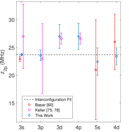
Figure 1: Relativistic core fine-structure SMS (MHz) in various configurations. Compared with the values obtained by Basar et. al. Basar et al. (1997), and Keller et. al. Keller (1973); Bauche and Keller (1971). The dashed line notes the value returned from the interconfiguration global fit of Sec. IX

.

IX Interconfiguration fit

The similar values of $z_{2p}$ of figure 1 indicate that combining them to a single parameter - the SMS in the Ne-II fine-structure, will improve the global fit. Another reduction of parameters is possible by taking the isotope-shift fine-structure analogy further, through assuming that the $g_{1}$ parameters of table 5 not only share the $G_{1}$ parameters’ angular coefficients, but also decrease with the same proportion:

$$\frac{g_{1}(2p,nl)}{g_{1}(2p,n^{\prime}l)}=\frac{G_{1}(2p,nl)}{G_{1}(2p,n^{\prime}l)}.$$ (10)

Figure 2 demonstrates the validity of equation 10 for the relevant configurations.

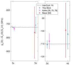
Figure 2: 1-order SMS parameters $g_{1}$ from table 5, and those deduced from Baser et. al. Basar et al. (1997), and Keller et. al. Bauche and Keller (1971); Keller (1973); Bauche and Champeau (1976). $g_{1}(nl)$ is scaled to $g_{1}(3l)$ according to the respective fine-structure exchange integrals using equation 10. The dashed line notes the value returned from the interconfiguration global fit of Sec. IX.

The above discussion leads to a global fit with $21$ parameters (table 6), and $\nu=124$ DOFs, which gives $\chi^{2}/\nu=0.930$. The value of the global core SMS parameter is shown in figure 1, and of the relevant $g_{1}(2p,3l)$ parameters in figure 2. As in Sec. VIII, the level RIS are recalculated and given in table 10, and show an average gain of $2.5$ in uncertainty between intra- and inter-configuration fit. Recalculating transition shifts from the parameters of table 6, and their correlations, results in an average gain of $27$.

The inter- and intraconfiguration effective RIS parameters of tables 5 and 6 offer an informed method of comparing the analyzed experimental results with theoretical calculations, since the latter usually did not account for one or more non-negligible effects.

Table 6: Effective IS parameters for inter-configuration global fit (MHz). Compared with table 5, the $z_{2p}$ parameters are fused together, and some $g_{1}$ parameters are deduced from Eq. 10.

	3s	3p	4s	3d	4p	5s	4d
$z_{2p}$	23.7(2)
$f_{0}$		419.4(7)	144(2)	244(2)	283(3)	186(1)	233(7)
$g_{1}$	-726(1)			-110(3)
$T(^{1}S)$		-87(2)			-32(2)
$T(^{3}S)$		130(2)			69(15)
$T(^{1}P)$		64(1)			14(2)
$T(^{1}D)$		45(1)			6(3)
$T(^{3}D)$		39.0(7)			16(1)
$c$		4.6(6)

X Comparison with theory

In this section we go over every theoretical effort made in the past to calculate neon isotope shift for the relevant transitions. We show that many large discrepancies are removed when reinterpreting the ab initio calculations of specific mass shifts as calculations of the effective parameters of tables 5 and 6, while taking into account the field shifts of table 1.

The first effort for calculating SMS effects in isotope shifts was undertaken by Bartlet and Gibbons in $1933$ Bartlett and Gibbons (1933). They used Hartree-Fock (HF) wavefunctions to evaluate the isotope shifts in neon $3s-3p$ transitions measured by Nagaoka (1930). Since LS-coupling was assumed, and no FS, core shift, and CSO effects were taken into account, their results may now be reinterpreted as a calculation of 1-order SMS parameters. Adapting their notations to the conventions of this work, and utilizing modern values for the neon and electron masses, their resulting LS SMS parameter: $g_{1}(3s)=$ $3s$ ${}^{1}P$ - $3s$ ${}^{3}P$ = $-589$ MHz, is now in a reasonable agreement, considering the number of HF functions used Ahmad (1985), with the value of $g_{1}(3s)=-726(1)$ MHz from table 6.

More recently, an MBPT calculation relying on the same assumptions as Bartlett and Gibbons (1933), including LS coupling, was attempted by Ahmad (1985). Thus it can not be directly compared with experiment in a meaningful way. Taking the difference between their value for the $3s$ ${}^{1}P-3p$ SMS, and $3s$ ${}^{3}P-3p$ SMS to the first-order of the computation (which is the only order expected to contribute to this value) returns a value of $g_{1}(3s)=-720$ MHz, which is agreement with our analysis to $1\%$. This agreement supports the fact that relativistic effects do not contribute substantially to SMS outside the core.

Other estimates of 1-order SMS parameters appear in the literature for parametric investigations in neon, and may be compared directly with the values appearing in tables 5 and 6. Our value of $g_{1}(3d)=-106(4)$ MHz, agrees with the value of $3d$ ${}^{1}P$ - $3d$ ${}^{3}P$ = $-96(6)$ MHz calculated by Keller and Lesprit (1973) using multiconfigurational Hartree-Fock (MCHF) computations Hartree et al. (1939), with uncertainty estimated from the difference between their results for two calculation methods. Our value of $g_{1}(4d)=-58(7)$ MHz agrees well with the value of $-58$ MHz computed by Bauche using the code of Fischer (1970), as it appears in Giacobino et al. (1979), however, our value of $g_{1}(5s)=-64(5)$ MHz is in less agreement with the calculated value of $-54$ MHz appearing in Giacobino et al. (1979).

As for the offset between configurations, both Bartlett and Gibbons (1933) and Ahmad (1985) calculated $3s-3p$ isotope shifts assuming no appreciable FS, which from table 1 is $9.5(1.0)$ MHz, and negligible differences within the $3p$ configuration, where from table 10, the differences are up to $200$ MHz. For comparison purposes, we compute the center of gravity of the $3p$ configuration relative to the reference level, by weighing each LS-parameter $T(^{2S+1}L)$ of table 6, by its multiplicity $w_{SL}=(2S+1)(2L+1)$. The resulting center configuration relative RIS is $\delta\nu_{\mathrm{RIS}}(3p)=f_{0}(3p)+\Sigma_{SL\neq^{3}P}w_{SL}T(^{2S+1}L)/\Sigma_{SL}w_{SL}=456(3)$ MHz. For comparing the SMS itself, we remove the relative field shift of $9.5$ MHz appreaing in table 1 to obtain a value of $\delta\nu_{\mathrm{SMS}}(3p)=447(3)$ MHz. This value is in reasonable agreement with the value of $3s$ ${}^{3}P$ $-3p$ $=410$ MHz of Bartlett and Gibbons (1933), and is in very good agreement with the value of $3s$ ${}^{3}P$ -$3p$ $=447$ MHz calculated by Ahmad (1985) to 1-order. 2-order SMS effects are not expected to contribute to the center of gravity shift. This agreement further validates that relativistic IS effects do not play a significant role outside of the core.

For relating the relativistic core fine-structure IS of our analysis with theory, the separation between NMS and SMS is not accurate, and the comparison is made by considering the total core fine-structure IS. Applying equation 2 to the Ne-II fine-structure interval of $780.424(2)$ cm^-1 Kramida and Nave (2006), we obtain a core fine-structure non-relativistic NMS of $58.35$ MHz, with negligible uncertainty. Adding to that the global SMS parameter $z_{2p}=23.72(16)$ from table 6, the total core fine-structure isotope shift is estimated as $82.07(16)$ MHz. This value compares well with a difficult, 4-order, MBPT calculation by Veseth, which under our sign convention results in $93(14)$ MHz, with the uncertainty evaluated as $10\%$ of the large CSO term in the calculation Veseth (1985a).

Since the optical electron is at rest at infinity, the RIS of all levels approaches zero with respect to the appropriate subconfiguration ionization limit. The $f_{0}$ values of table 6 represent the RIS of pure $j_{\mathrm{c}}=3/2$,${}^{3}P$ states, which for $ns,nd$ configurations is a non-relativistic, 1-order effect and expected to approach zero in an ordinary (polynomial) manner. From this convergence rate, a crude estimation of the absolute RIS of the reference level is $210(20)$ MHz, resulting in an absolute RIS of the ground level of $-9392(23)$ MHz. From the fast convergence of the FS-factors to the ionization limit (table 1), we assume that the absolute field shift of $4f$ state is negligible, and so estimate the absolute FS of the ground level by $\delta\nu_{\mathrm{FS}}$(${}^{1}S_{0})=-35(4)$ MHz, giving an absolute $\delta\nu_{\mathrm{SMS}}$(${}^{1}P_{0})=-9358(23)$ MHz. This value agrees to some extent with the calculated value of $-10.1$ GHz calculated by Veseth (1985b), if we follow Eikema et al. (1994) in estimating the calculation uncertainty as $0.5$ GHz.

To conclude this section we review the only available direct calculation of various IS effects for a specific transition, namely the $614.3$ nm transition between our reference level $3s[3/2]_{2}$ and the $3p[3/2]_{2}$ level Li et al. (2016). This line isotope shift is of high interest for nuclear physics, since it was measured precisely for various neon isotopes, including the two-proton halo candidate, ¹⁷Ne Geithner et al. (2008b); Marinova et al. (2011), and determines the RMS charge radii difference between them. The calculation method used was multiconfigurational Dirac-Hartree-Fock (MCDHF), including Breit interactions and not including other relativistic corrections. A direct comparison with the shifts observed in experiment, for which the uncertainty was $1-3$ MHz, yielded discrepancies from $15$ to $97$ MHz (see table 4 in Li et al. (2016)).

Table 7: Isotope shift effective parameters compared with theoretical calculations. The first lines reinterpret calculations of mass shifts within configurations as those of effective $g_{1}$ parameters from tables 5 and 6. The following lines reinterpret calculations of interconfiguration offsets utilizing the field shifts of table 1. All values are in MHz.

Parameter	This Work	Theory	Ref.	Method
$g_{1}(3s)$	-726(1)	-720	Ahmad (1985)	MBPT
		-591	Bartlett and Gibbons (1933)	HF
$g_{1}(3d)$	-106(4)	-96	Keller (1973)	MCHF
$g_{1}(4d)$	-58(7)	-58	Giacobino et al. (1979)	MCHF
$g_{1}(5s)$	-64(5)	-54	Giacobino et al. (1979)	MCHF
$\delta\nu_{\mathrm{SMS}}(3s$ ${}^{3}P_{2}-3p)$	447(3)	447	Ahmad (1985)	MBPT
		410	Bartlett and Gibbons (1933)	HF
$\delta\nu$(fine structure)	82.1(2)	93	Veseth (1985a)	MBPT
$\delta\nu_{\mathrm{SMS}}$(Core-Ionization limit)	-9359(23)	-10110	Veseth (1985b)	MBPT
$\delta\nu(3s$ ${}^{3}P_{2}-3p[3/2]_{2})$	1663.8(2)	1668	Li et al. (2016)	MCDHF

These discrepancies are to a large extent removed upon reanalysis of the theory. After reversing the sign of the field shifts of table 4 in Li et al. (2016), the discrepancies are even larger for all isotopes, and vary between $30$ and $110$ MHz. Another large correction is related to the Breit interaction. In this work we demonstrated that relativistic effects are mostly confined to the core, where the unaccounted-for relativistic corrections to the mass shift operators cancel the Breit interaction to a large extent Veseth (1985a). Moreover, the $3s[3/2]_{2}$ level is completely related to the $j_{\mathrm{c}}=3/2$ core, and the $3p[3/2]_{2}$ level is $89\%$ related to this core (see table 12). We thus exchange the Breit correction of $9$ GHz u ($27$ MHz for ^20,22Ne) of table 3 in Li et al. (2016), with the much smaller value of $0.57$ GHz u, corresponding to a $11\%\times z(2p)=2.6$ MHz for ^20,22Ne core shift. After application of both corrections, and assessing the theoretical uncertainty as at least the last presented digit, an agreement between experiment and theory is achieved for all neon isotopes. The corrected theoretical value for ^20,22Ne is $1668(5)$ and agrees with the value measured by Geithner et al. (2008b) of $1663.6(1.7)$ MHz, and the updated value from this work of $1663.8(2)$.

An overview of table 7 demonstrates that when relativistic effects do not play a key role, i.e. outside of the core, MBPT and MCHF methods handle multielectron correlations much better than is most often claimed Marinova (2015), at least for the case of neon transitions.

XI Conclusion and outlook

XI.1 Neon charge radii

In this work we calculated the field-shift factors for a variety of neon transitions with an accuracy of a few percent. These values are used in updating the RMS charge radii differences for a multitude of neon isotopes, as well as facilitating a comparison of mass shift parameters with theoretical calculations.

Following our update, the limiting factor for determining neon charge radii differences is the systematic uncertainty in the modified King-plot procedure stemming from the calibration of absolute ^20-22Ne radii measurements. A better calibration of the slope is obtained provided that $\delta\langle r^{2}\rangle^{20,22}$ is known with higher precision. Whereas we elected to use the same, nuclear-model dependent, value for $\delta\langle r^{2}\rangle^{20,22}$ that is used by Geithner et al. (2008b); Marinova et al. (2011), other determinations appear in the literature Fricke et al. (2004), which indicate that the isotope shifts are not as well-understood as claimed and may benefit from further discussion.

Conversely, if relativistic calculations on many electron correlations reach a point where it is possible to predict the specific mass shift for any of the most accurately known neon transitions (i.e. the $640$ nm cooling transition, between levels which have the same core) to an accuracy of roughly $200$ kHz, then $\delta\langle r^{2}\rangle^{20,22}$ may be deduced directly from the isotope shift without a King plot procedure. This would remove systematic uncertainties in $\delta\langle r^{2}\rangle^{20,A}$, which are up to an order of magnitude greater than the statistical uncertainty in the IS measurements. Such an effort is under way.

XI.2 Dual Sideband Spectroscopy

We measured the isotope shifts of seven transitions with an accuracy of $<10^{-4}$. The consistency of experimental results demonstrates that dual sideband spectroscopy is a simple and precise technique for obtaining the frequency differences between far resonances, and removes frequency noise and nonlinear scanning effects.

Utilizing this technique a substantially shorter laser frequency scan is possible, which may be beneficial in the spectroscopy of short lived radioisotopes Campbell et al. (2016). We plan to combine this technique with metastable quenching spectroscopy Ohayon et al. (2015), for hyperfine and isotope shift measurements of various neon isotopes produced at the SARAF particle accelerator Ohayon et al. (2018); Mardor et al. (2018).

XI.3 Parametric analysis and global fit

The great body of isotope shift data, which is available only for neon and analyzed in this work, provides a unique opportunity for developing new methods for classifying and understanding the various relativistic, electronic and nuclear effects which donate to the lineshifts.

The parametric investigation employed here, allows to disentangle the complex intermediate coupling of neon levels, and enables to describe $145$ average transition isotope shifts through $21$ effective parameters which are either purely jj or LS-coupled. Recalculating neon levelshifts from these parameters results in a substantial increase in precision. This database of precise neon isotope shifts from $80-8000$ nm may be used for calibration of collinear laser spectroscopy experiments at various accelerator facilities Gebert et al. (2015).

Even though our reanalysis demonstrates that specific mass shift calculations in neon preform better than common knowledge, still their limited accuracy is the limiting factor for most charge radii difference determinations, in neon and other multielectron elements Marinova (2015); Gebert et al. (2015). We propose that new, relativistic ab initio mass shift calculations are preformed for a large number of levels, analyzed in the intermediate coupling framework, and compared to experimental observables in a parametric basis.

Appendix

This appendix contains the inputs to, and outputs from, our global analysis. Tables 8 and 9 contain the experimental transition isotope shifts used. Their averaging procedure is discussed in Sec. V. Tables 10 and 11, present the extracted residual isotope shift (RIS) of levels and their correlations, respectively, relative to the the reference level $3s[3/2]_{2}$, and discussed in Sec. VI. The angular coefficients, calculated according the procedure outlined in Sec. VII, are presented in table 12. These coefficients are used for calculation of level shifts for the two fitting procedures outlined in sections VIII, and IX.

Table 8: Measured isotope shifts in MHz for transitions with air wavelength of 60-600 nm. ‘Mean’ column is the dispersion-corrected weighted average. ‘Calc’ are the calculated shifts from fitting equation 5.

$\lambda$	From	To	Ritschl (1937); Biraben et al. (1975); Giacobino et al. (1979); Eikema et al. (1994); Rupper and Merkt (2004)	Saprykin et al. (2015); Saprykin (2016, 2017)	Mean IS	Calculated IS
62.95	${}^{1}S_{0}$	$4s$ $[3/2]_{1}$	2159(90)	2305(20)	2298(31)	2309(29)
73.57	${}^{1}S_{0}$	$3s$’$[1/2]_{1}$	-90(90)	-98(16)	-98(16)	-99(11)
74.35	${}^{1}S_{0}$	$3s$ $[3/2]_{1}$	420(90)	417(16)	417(16)	415(11)
296.07	$3s$ $[3/2]_{2}$	$4d$’$[3/2]_{1}$	2764.6(3.0)		2764.6(3.0)	2764.2(3.0)
296.16	$3s$ $[3/2]_{2}$	$4d$’$[3/2]_{2}$	2779.2(4.0)		2779.2(4.0)	2778.1(3.8)
296.17	$3s$ $[3/2]_{2}$	$4d$’$[5/2]_{3}$	2780.1(1.3)		2780.1(1.3)	2780.2(1.3)
296.18	$3s$ $[3/2]_{2}$	$4d$’$[5/2]_{2}$	2781.8(2.0)		2781.8(2.0)	2781.8(2.0)
302.88	$3s$ $[3/2]_{2}$	$4d$ $[5/2]_{3}$	2701.4(2.4)		2701.4(2.4)	2702.5(2.3)
302.89	$3s$ $[3/2]_{2}$	$4d$ $[5/2]_{2}$	2702.5(5.0)		2702.5(5.0)	2702.0(4.8)
303.08	$3s$ $[3/2]_{2}$	$4d$ $[3/2]_{1}$	2668.7(5.0)		2668.7(5.0)	2668.6(4.9)
303.22	$3s$ $[3/2]_{2}$	$4d$ $[3/2]_{2}$	2699.3(2.1)		2699.3(2.1)	2698.4(2.1)
303.31	$3s$ $[3/2]_{2}$	$4d$ $[7/2]_{3}$	2696.1(5.2)		2696.1(5.2)	2696.1(4.9)
303.32	$3s$ $[3/2]_{2}$	$4d$ $[7/2]_{4}$	2697.0(3.6)		2697.0(3.6)	2697.0(3.6)
303.55	$3s$ $[3/2]_{2}$	$4d$ $[1/2]_{1}$	2686.0(2.6)		2686.0(2.6)	2686.0(2.6)
306.52	$3s$ $[3/2]_{2}$	$5s$’$[1/2]_{1}$	2621.4(2.3)		2621.4(2.3)	2620.7(2.1)
306.99	$3s$ $[3/2]_{2}$	$5s$’$[1/2]_{0}$	2646.8(3.6)		2646.8(3.6)	2646.6(3.6)
313.67	$3s$ $[3/2]_{2}$	$5s$ $[3/2]_{1}$	2532.5(3.0)		2532.5(3.0)	2532.6(3.0)
314.51	$3s$ $[3/2]_{2}$	$5s$ $[3/2]_{2}$	2562.1(2.4)		2562.1(2.4)	2562.1(2.4)
336.98	$3s$ $[3/2]_{2}$	$4p$’$[3/2]_{2}$	2488(90)		2488(90)	2532.9(3.2)
336.99	$3s$ $[3/2]_{2}$	$4p$’$[1/2]_{1}$	2488(90)		2488(90)	2537.1(4.9)
344.77	$3s$ $[3/2]_{2}$	$4p$ $[3/2]_{2}$	2428(90)		2428(90)	2380(37)
345.07	$3s$ $[3/2]_{2}$	$4p$ $[3/2]_{1}$	2548(90)		2548(90)	2436(47)
345.41	$3s$ $[3/2]_{1}$	$4p$ $[1/2]_{0}$	2488(90)		2488(90)	2462(40)
346.04	$3s$’$[1/2]_{0}$	$4p$’$[3/2]_{2}$	2548(90)		2548(90)	2451.1(3.2)
346.43	$3s$ $[3/2]_{2}$	$4p$ $[5/2]_{2}$	2518(90)		2518(90)	2446.2(6.6)
346.65	$3s$’$[1/2]_{0}$	$4p$’$[3/2]_{1}$	2428(90)		2428(90)	2456.0(6.3)
347.25	$3s$ $[3/2]_{2}$	$4p$ $[5/2]_{3}$	2518(90)		2518(90)	2488(77)
349.80	$3s$ $[3/2]_{1}$	$4p$ $[3/2]_{2}$	2398(90)		2398(90)	2390(37)
350.12	$3s$ $[3/2]_{1}$	$4p$ $[3/2]_{1}$	2488(90)		2488(90)	2446(47)
351.07	$3s$ $[3/2]_{2}$	$4p$ $[1/2]_{1}$	2518(90)		2518(90)	2499(64)
351.51	$3s$ $[3/2]_{1}$	$4p$ $[5/2]_{2}$	2518(90)		2518(90)	2456.1(6.6)
352.04	$3s$’$[1/2]_{1}$	$4p$’$[1/2]_{0}$	3178(90)		3178(90)	3039(40)
360.01	$3s$’$[1/2]_{1}$	$4p$’$[3/2]_{1}$	3088(90)		3088(90)	3061.7(6.5)
360.91	$3s$’$[1/2]_{0}$	$4p$ $[1/2]_{1}$	2398(90)		2398(90)	2417(64)
363.36	$3s$’$[1/2]_{1}$	$4p$ $[1/2]_{0}$	3118(90)		3118(90)	2976(40)
368.22	$3s$’$[1/2]_{1}$	$4p$ $[3/2]_{2}$	2878(90)		2878(90)	2904(37)
368.57	$3s$’$[1/2]_{1}$	$4p$ $[3/2]_{1}$	2818(90)		2818(90)	2960(47)
370.12	$3s$’$[1/2]_{1}$	$4p$ $[5/2]_{2}$	3058(90)		3058(90)	2970.0(6.7)

			Nagaoka (1930); Ritschl (1937); Schober (1939)	Odintsov (1965)	Wik et al. (1978)	Belfrage et al. (1983); Lindsay et al. (1991)	Delsart and Keller (1975); Bergquist ; Gerstenberger et al. (1988); Bielski et al. (1991)	Konz et al. (1992); Cheng and Shy (2000)	Guthöhrlein and Windholz (1995)	Ståhlberg et al. (1989); Basar et al. (1997)	Mean IS	Calculated IS
511.4	$3p$ $[1/2]_{1}$	$4d$’$[3/2]_{1}$	899(150)								899(150)	1148.5(3.5)
532.6	$3p$ $[1/2]_{1}$	$4d$ $[3/2]_{1}$	989(90)								989(90)	1052.9(5.2)
533.1	$3p$ $[1/2]_{1}$	$4d$ $[3/2]_{2}$	1229(90)								1229(90)	1082.7(2.8)
534.1	$3p$ $[1/2]_{1}$	$4d$ $[1/2]_{1}$	1139(90)								1139(90)	1070.3(3.2)
534.3	$3p$ $[1/2]_{1}$	$4d$ $[1/2]_{0}$	929(90)								929(90)	929(90)
540.0	$3s$ $[3/2]_{1}$	$3p$’$[1/2]_{0}$	1829(90)				1802(27)				1804(26)	1772.4(2.4)
543.4	$3p$ $[1/2]_{1}$	$5s$’$[1/2]_{1}$	809(90)				1000(50)	1014.0(5.0)			1013.2(8.0)	1004.5(2.7)
544.8	$3p$ $[1/2]_{1}$	$5s$’$[1/2]_{0}$	899(90)								899(90)	1030.9(4.1)
556.2	$3p$ $[5/2]_{2}$	$4d$’$[3/2]_{2}$	989(150)								989(150)	1137.1(3.8)
565.2	$3p$ $[3/2]_{1}$	$4d$’$[3/2]_{1}$	869(150)								869(150)	1094.7(3.0)
565.7	$3p$ $[3/2]_{1}$	$4d$’$[5/2]_{2}$								1120(30)	1120(30)	1112.4(2.0)
566.2	$3p$ $[1/2]_{1}$	$5s$ $[3/2]_{1}$	839(90)								839(90)	916.9(3.5)
569.0	$3p$ $[1/2]_{1}$	$5s$ $[3/2]_{2}$	959(90)							940(30)	942(28)	946.4(3.0)
571.9	$3p$ $[3/2]_{2}$	$4d$’$[5/2]_{3}$								1120(30)	1120(30)	1116.2(1.3)
574.8	$3p$ $[5/2]_{3}$	$4d$ $[5/2]_{3}$								1093(12)	1093(12)	1076.5(2.3)
576.0	$3p$ $[5/2]_{3}$	$4d$ $[3/2]_{2}$								1047(11)	1047(11)	1072.4(2.1)
576.4	$3p$ $[5/2]_{3}$	$4d$ $[7/2]_{4}$								1070(30)	1070(30)	1071.0(3.6)
580.4	$3p$ $[5/2]_{2}$	$4d$ $[5/2]_{2}$								1070(30)	1070(30)	1061.0(4.8)
582.0	$3p$ $[5/2]_{2}$	$4d$ $[7/2]_{3}$	929(90)							1070(20)	1063(30)	1055.2(4.9)
585.2	$3s$’$[1/2]_{1}$	$3p$’$[1/2]_{0}$	2248(90)	2287.4(3.0)	2276.0(7.0)	2300(15)			2298(20)		2286.3(2.7)	2286.1(2.2)
587.3	$3p$’$[3/2]_{1}$	$4d$’$[5/2]_{2}$								1060(20)	1060(20)	1053.1(2.0)
588.2	$3s$ $[3/2]_{2}$	$3p$’$[1/2]_{1}$	1709(90)	1738.8(3.0)	1736.6(1.8)	1740(2)	1736.7(6)	1738(6)	1736.0(5.0)		1736.97(53)	1736.93(51)
590.2	$3p$’$[3/2]_{2}$	$4d$’$[5/2]_{3}$								1070(20)	1070(20)	1064.4(1.6)
590.3	$3p$’$[3/2]_{2}$	$4d$’$[5/2]_{2}$								1061(18)	1061(18)	1066.1(2.2)
590.6	$3p$ $[3/2]_{1}$	$4d$ $[5/2]_{2}$	1019(150)							1020(20)	1020(20)	1032.5(4.8)
591.3	$3p$ $[3/2]_{1}$	$4d$ $[3/2]_{1}$	779(150)							1002(14)	1000(21)	999.1(4.9)
591.9	$3p$ $[1/2]_{0}$	$4d$’$[3/2]_{1}$	959(150)							1070(30)	1066(29)	1072.8(3.8)
594.5	$3s$ $[3/2]_{2}$	$3p$’$[3/2]_{2}$	1679(90)	1714.8(3.0)	1716.4(1.4)	1717(3)	1731(12)	1714(4)	1714.3(5.0)	1712(8)	1716.0(1.1)	1715.77(94)
596.1	$3p$’$[1/2]_{1}$	$4d$’$[3/2]_{1}$								1020(20)	1020(20)	1027.2(3.0)
596.5	$3p$’$[1/2]_{1}$	$4d$’$[3/2]_{2}$								1029(14)	1029(14)	1041.2(3.9)
597.4	$3p$ $[3/2]_{2}$	$4d$ $[5/2]_{3}$								1070(20)	1070(20)	1038.5(2.3)
597.5	$3s$ $[3/2]_{2}$	$3p$’$[3/2]_{1}$	1649(90)		1730.0(3.7)	1728(5)		1725(3)	1727.3(5.0)	1734(11)	1727.4(1.9)	1728.78(21)
598.8	$3p$ $[3/2]_{2}$	$4d$ $[3/2]_{2}$	1109(150)							1030(20)	1031(20)	1034.4(2.1)
599.2	$3p$ $[3/2]_{2}$	$4d$ $[7/2]_{3}$								1030(16)	1030(16)	1032.1(4.9)

Table 9: Measured isotope shifts in MHz for transitions with air wavelength of 600-10,000 nm. ‘Mean’ column is the dispersion-corrected weighted average. ‘Calculated’ are the calculated shifts from fitting equation 5. Ouliers are italicized.

$\lambda$	From	To	Ritschl (1937); Schober (1939); Cordover et al. (1965)	Odintsov (1965); Zory (1966)	Schweitzer Jr (1968); Delsart and Keller (1975); Julien et al. (1980); Belfrage et al. (1983)	Ståhlberg et al. (1989); Lindsay et al. (1991); Konz et al. (1992)	Ballik (1972); Guthöhrlein and Windholz (1995)	Kotlikov and Tokarev (1980); Basar et al. (1997)	Vernyi and Sokolova (1967); Ducas et al. (1972); Zhao (1987); Geithner et al. (2008a)	This Work	Mean	Calculated
600.1	$3p$ $[3/2]_{2}$	$4d$ $[1/2]_{1}$						1020(20)			1020(20)	1022.0(2.6)
603.0	$3s$ $[3/2]_{1}$	$3p$’$[1/2]_{1}$	1709(90)				1743.5(5.0)	1746(17)			1743.6(4.8)	1747.18(53)
607.4	$3s$ $[3/2]_{1}$	$3p$ $[1/2]_{0}$	1679(90)	1702.8(3.0)			1700.5(5.0)	1695(17)			1702.0(2.5)	1701.6(2.5)
609.6	$3s$ $[3/2]_{1}$	$3p$’$[3/2]_{2}$	1679(90)	1726.8(3.0)	1740(12)	1753(8)	1720.0(5.0)	1722(17)	1708(26)		1725.3(2.5)	1726.03(95)
612.8	$3s$ $[3/2]_{1}$	$3p$’$[3/2]_{1}$					1737.5(2.0)	1745(16)			1737.6(2.0)	1739.04(25)
614.3	$3s$ $[3/2]_{2}$	$3p$ $[3/2]_{2}$	1649(90)	1660.9(3.0)	1669(4)	1660(3)	1663.7(5.0)	1653(14)	1663.6(1.7)		1663.0(1.2)	1664.01(25)
616.3	$3s$’$[1/2]_{0}$	$3p$’$[1/2]_{1}$	1649(90)	1651.9(3.0)	1663(5)	1665(5)	1653.8(5.0)				1656.4(2.8)	1655.19(54)
618.2	$3p$ $[5/2]_{3}$	$5s$ $[3/2]_{2}$	1019(90)								1019(90)	936.1(2.4)
621.7	$3s$ $[3/2]_{2}$	$3p$ $[3/2]_{1}$	1679(150)			1674(3)	1666.3(5.0)		1669.43(8)		1669.43(8)	1669.43(8)
624.7	$3p$ $[5/2]_{2}$	$5s$ $[3/2]_{2}$	869(150)								869(150)	921.1(2.4)
625.9	$3p$’$[1/2]_{1}$	$4d$ $[3/2]_{2}$	1079(150)								1079(150)	961.5(2.1)
626.6	$3s$’$[1/2]_{0}$	$3p$’$[3/2]_{1}$	1619(90)	1645.9(3.0)	1651(3)	1658(3)	1649.5(5.0)		1646.92(9)	1647.37(14)	1647.05(10)	1647.05(10)
630.5	$3s$ $[3/2]_{1}$	$3p$ $[3/2]_{2}$	1649(90)	1675.8(3.0)			1679.0(5.0)			1674.27(19)	1674.28(19)	1674.26(19)
632.8	$3p$’$[3/2]_{2}$	$5s$’$[1/2]_{1}$	875(12)	909(15)	901(20)	904(8)	1052(100)	889(9)	684(60)		895.5(6.1)	904.4(2.2)
633.4	$3s$ $[3/2]_{2}$	$3p$ $[5/2]_{2}$	1619(90)			1650(3)	1651.9(5.0)		1640.91(11)	1641.05(16)	1640.96(12)	1640.97(11)
638.3	$3s$ $[3/2]_{1}$	$3p$ $[3/2]_{1}$	1709(90)	1681.8(3.0)			1683.0(5.0)			1679.60(26)	1679.63(26)	1679.68(17)
640.2	$3s$ $[3/2]_{2}$	$3p$ $[5/2]_{3}$	1709(90)	1627.9(3.0)	1630(3)	1632(3)	1631.2(5.0)	1629.5(1.0)	1625.93(12)	1626.05(11)	1626.01(09)	1626.01(09)
644.5	$3p$ $[3/2]_{2}$	$5s$ $[3/2]_{2}$	899(150)								899(150)	898.1(2.4)
650.6	$3s$ $[3/2]_{1}$	$3p$ $[5/2]_{2}$	1709(90)	1645.9(3.0)			1653.1(5.0)	1653(2)		1651.25(17)	1651.25(18)	1651.22(15)
653.3	$3s$’$[1/2]_{0}$	$3p$ $[3/2]_{1}$	1679(90)	1585.9(3.0)		1607(6)	1597.9(5.0)	1588(3)	1587.54(11)	1588.24(22)	1587.68(16)	1587.69(16)
659.9	$3s$’$[1/2]_{1}$	$3p$’$[1/2]_{1}$	2129(90)	2263.4(3.0)			2257.9(5.0)	2259(2)			2260.1(1.8)	2260.8(1.3)
665.2	$3s$’$[1/2]_{1}$	$3p$ $[1/2]_{0}$					2201(20)	2190(20)			2196(14)	2215.2(2.8)
667.8	$3s$’$[1/2]_{1}$	$3p$’$[3/2]_{2}$	2129(90)	2236.5(3.0)		2230(6)	2218.8(5.0)				2231.4(4.4)	2239.7(1.5)
671.7	$3s$’$[1/2]_{1}$	$3p$’$[3/2]_{1}$	2099(90)	2257.4(3.0)			2256.0(3.0)				2256.6(2.7)	2252.7(1.3)
692.9	$3s$’$[1/2]_{1}$	$3p$ $[3/2]_{2}$	2159(90)	2188.5(3.0)			2199.8(5.0)				2191.5(3.6)	2187.9(1.3)
702.4	$3s$’$[1/2]_{1}$	$3p$ $[3/2]_{1}$					2180(20)				2180(20)	2193.3(1.3)
703.2	$3s$ $[3/2]_{2}$	$3p$ $[1/2]_{1}$	1649(90)	1615.9(3.0)			1616.3(5.0)				1616.0(2.6)	1615.7(1.9)
717.4	$3s$’$[1/2]_{1}$	$3p$ $[5/2]_{2}$	2039(90)				2134(20)				2130(20)	2164.9(1.3)
724.5	$3s$ $[3/2]_{1}$	$3p$ $[1/2]_{1}$	1529(150)				1626.7(3.0)				1626.7(3.0)	1626.0(1.9)
743.9	$3s$’$[1/2]_{0}$	$3p$ $[1/2]_{1}$	1439(90)								1439(90)	1534.0(1.9)
748.9	$3p$ $[1/2]_{1}$	$3d$ $[3/2]_{2}$	600(90)								600(90)	617(37)
753.6	$3p$ $[1/2]_{1}$	$3d$ $[1/2]_{1}$	570(90)								570(90)	548(69)
754.4	$3p$ $[1/2]_{1}$	$3d$ $[1/2]_{0}$	690(90)								690(90)	690(90)
783.3	$3p$ $[5/2]_{3}$	$3d$’$[3/2]_{2}$						780(30)			780(30)	766.1(5.1)
783.9	$3p$ $[5/2]_{3}$	$3d$’$[5/2]_{3}$						670(30)			670(30)	762.7(3.3)

			Ritschl (1937); Schober (1939); Szöke and Javan (1963); Sakurai et al. (1966)	Cordover et al. (1967)	Ducas et al. (1972)	Ballik (1972); Ohi (1973)	Keller (1973); Delsart and Keller (1975); Sasada and Kubota (1992)	Mean	Calculated
813.6	$3p$ $[3/2]_{1}$	$3d$’$[5/2]_{2}$	570(150)					570(150)	722.1(6.4)
837.7	$3p$ $[5/2]_{3}$	$3d$ $[7/2]_{4}$	630(150)					630(150)	714(77)
849.5	$3p$ $[5/2]_{2}$	$3d$ $[7/2]_{3}$	630(90)					630(90)	657.4(6.7)
859.1	$3p$’$[3/2]_{1}$	$3d$’$[5/2]_{2}$	510(150)					510(150)	662.8(6.4)
863.4	$3p$ $[3/2]_{1}$	$3d$ $[5/2]_{2}$	600(150)					600(150)	618(47)
865.4	$3p$’$[3/2]_{2}$	$3d$’$[5/2]_{3}$	420(150)					420(150)	672.9(3.4)
878.0	$3p$ $[3/2]_{2}$	$3d$ $[5/2]_{3}$	600(150)					600(150)	576(37)
878.4	$3p$’$[1/2]_{1}$	$3d$’$[3/2]_{2}$	420(150)					420(150)	655.1(5.1)
886.5	$3p$ $[1/2]_{1}$	$4s$’$[1/2]_{1}$	210(150)					210(150)	360.7(2.8)
886.6	$3p$ $[3/2]_{2}$	$3d$ $[7/2]_{3}$	570(90)					570(90)	634.4(6.7)
914.8	$3p$’$[3/2]_{1}$	$3d$ $[5/2]_{2}$	540(150)					540(150)	558(47)
920.2	$3p$’$[3/2]_{1}$	$3d$ $[3/2]_{1}$	360(90)					360(90)	495(40)
922.0	$3p$’$[3/2]_{2}$	$3d$ $[5/2]_{3}$	600(150)					600(150)	524(37)
922.6	$3p$’$[3/2]_{1}$	$3d$ $[3/2]_{2}$	510(150)					510(150)	503(37)
930.1	$3p$’$[3/2]_{2}$	$3d$ $[3/2]_{2}$	480(150)					480(150)	516(37)
932.6	$3p$ $[1/2]_{0}$	$3d$ $[3/2]_{1}$	360(90)					360(90)	532(40)
942.5	$3p$ $[1/2]_{0}$	$3d$ $[1/2]_{1}$	420(150)					420(150)	472(69)
945.9	$3p$’$[1/2]_{1}$	$3d$ $[3/2]_{2}$	390(150)					390(150)	495(37)
948.6	$3p$ $[1/2]_{1}$	$4s$ $[3/2]_{1}$	360(90)					360(90)	268(31)
953.4	$3p$’$[1/2]_{1}$	$3d$ $[1/2]_{1}$	420(150)					420(150)	427(69)
966.5	$3p$ $[1/2]_{1}$	$4s$ $[3/2]_{2}$	510(90)					510(90)	510(90)
1152	$3p$’$[3/2]_{2}$	$4s$’$[1/2]_{1}$	261(3)	257(8)	261(5)	257(25)	259.5(4.2)	260.3(2.1)	260.6(1.9)
1523	$3p$’$[1/2]_{0}$	$4s$’$[1/2]_{1}$					215.0(3.0)	215.0(3.0)	214.3(2.3)
3317	$4p$ $[5/2]_{2}$	$5s$ $[3/2]_{1}$					86.9(6.0)	86.9(6.0)	86.4(5.9)
3333	$4p$’$[3/2]_{1}$	$5s$’$[1/2]_{1}$					82.4(6.0)	82.4(6.0)	82.9(6.0)
3390	$4p$’$[1/2]_{1}$	$5s$’$[1/2]_{1}$					83.6(4.5)	83.6(4.5)	83.7(4.4)
3391	$4p$’$[3/2]_{2}$	$5s$’$[1/2]_{1}$	63(13)			90.3(1.6)	84.8(1.5)	87.2(2.4)	87.8(2.4)
3773	$3d$ $[3/2]_{1}$	$4p$’$[1/2]_{0}$					291.4(1.5)	291.4(1.5)	291.4(1.5)
5403	$3d$’$[3/2]_{1}$	$4p$’$[1/2]_{0}$					175.7(0.6)	175.7(0.6)	175.7(0.6)
5665	$3d$ $[3/2]_{1}$	$4p$ $[1/2]_{0}$					228.4(1.3)	228.4(1.3)	228.5(1.3)
6985	$3d$ $[3/2]_{2}$	$4p$ $[3/2]_{2}$					147.8(0.9)	147.8(0.9)	147.8(0.9)
7477	$3d$ $[5/2]_{3}$	$4p$ $[3/2]_{2}$					140.0(0.9)	140.0(0.9)	140.0(0.9)
7614	$3d$ $[5/2]_{2}$	$4p$ $[3/2]_{1}$					148.4(0.6)	148.4(0.6)	148.4(0.6)
7648	$3d$ $[7/2]_{3}$	$4p$ $[5/2]_{2}$					147.8(0.9)	147.8(0.9)	147.8(0.9)
7699	$3d$’$[5/2]_{3}$	$4p$’$[3/2]_{2}$					143.6(0.9)	143.6(0.9)	143.7(0.9)
7763	$3d$’$[3/2]_{2}$	$4p$’$[1/2]_{1}$					144.5(1.5)	144.5(1.5)	144.5(1.5)
8006	$3d$’$[5/2]_{2}$	$4p$’$[3/2]_{1}$					145.7(1.2)	145.7(1.2)	145.7(1.2)
8059	$3d$ $[7/2]_{4}$	$4p$ $[5/2]_{3}$					147.2(0.6)	147.2(0.6)	147.2(0.6)

Table 10: Residual isotope shifts in MHz, relative to the reference level. The 1 column is obtained from fitting Eq. 5, and the last two columns by fitting Eq. 9 utilizing the models of Sec. VIII and IX.

	Direct calculation	Intraconf. fit	Interconf. fit
Parameters:	55	30	21
DOF	90	115	124
Chi2/DOF	0.987	0.937	0.930
Relative AIC	42	10	0
$S_{0}$	9597(11)	9598(11)	9602(11)
$3s$ $[3/2]_{2}$	0	0	0
$3s$ $[3/2]_{1}$	-41.47(17)	-41.74(10)	-41.74(10)
$3s$’$[1/2]_{0}$	23.65(18)	23.72(17)	23.72(16)
$3s$’$[1/2]_{1}$	-662.0(1.3)	-660.7(1.1)	-660.7(1.1)
$3p$ $[1/2]_{1}$	552.8(1.9)	552.8(1.9)	552.8(1.9)
$3p$ $[5/2]_{3}$	458.449(92)	458.427(86)	458.420(76)
$3p$ $[5/2]_{2}$	460.91(11)	460.81(10)	460.81(10)
$3p$ $[3/2]_{1}$	467.129(78)	467.151(72)	467.156(70)
$3p$ $[3/2]_{2}$	447.18(25)	446.96(21)	446.96(20)
$3p$’$[3/2]_{1}$	477.85(21)	477.89(19)	477.89(17)
$3p$’$[3/2]_{2}$	458.38(94)	458.04(66)	458.12(32)
$3p$ $[1/2]_{0}$	429.5(2.5)	428.25(75)	428.28(71)
$3p$’$[1/2]_{1}$	466.08(51)	466.18(51)	466.18(51)
$3p$’$[1/2]_{0}$	346.8(2.4)	347.6(2.3)	347.6(2.3)
$4s$ $[3/2]_{2}$	289(90)	289(90)	143.7(1.9)
$4s$ $[3/2]_{1}$	33(31)	33(31)	69.9(1.9)
$4s$’$[1/2]_{1}$	70.3(2.0)	70.3(2.0)	70.3(1.9)
$3d$ $[1/2]_{0}$	251(90)	241.1(3.2)	244.2(2.3)
$3d$ $[1/2]_{1}$	109(69)	221.7(3.0)	224.0(2.4)
$3d$ $[7/2]_{4}$	281(77)	241.1(3.2)	244.2(2.3)
$3d$ $[7/2]_{3}$	238.4(6.7)	241.1(3.2)	244.2(2.3)
$3d$ $[3/2]_{2}$	171(37)	241.7(3.1)	244.7(2.3)
$3d$ $[3/2]_{1}$	160(40)	182.9(3.1)	183.9(2.8)
$3d$ $[5/2]_{2}$	219(47)	241.3(3.1)	244.4(2.3)
$3d$ $[5/2]_{3}$	172(37)	241.3(3.1)	244.4(2.3)
$3d$’$[5/2]_{2}$	270.5(6.4)	267.9(2.6)	267.7(2.3)
$3d$’$[5/2]_{3}$	267.6(3.3)	267.9(2.6)	267.7(2.3)
$3d$’$[3/2]_{2}$	270.2(5.1)	267.6(2.6)	267.4(2.3)
$3d$’$[3/2]_{1}$	216(40)	239.4(2.9)	238.2(2.5)
$4p$ $[1/2]_{1}$	370(64)	344(15)	347(13)
$4p$ $[5/2]_{3}$	335(77)	295.6(3.2)	298.6(2.4)
$4p$ $[5/2]_{2}$	288.5(6.6)	291.2(3.3)	294.3(2.3)
$4p$ $[3/2]_{1}$	270(47)	291.6(3.2)	294.6(2.4)
$4p$ $[3/2]_{2}$	212(37)	282.0(3.1)	284.8(2.4)
$4p$ $[1/2]_{0}$	257(40)	279.2(2.9)	280.9(2.6)
$4p$’$[3/2]_{1}$	322.9(6.3)	320.4(2.7)	320.3(2.3)
$4p$’$[1/2]_{1}$	318.4(4.9)	316.2(2.8)	316.1(2.6)
$4p$’$[3/2]_{2}$	314.2(3.2)	314.5(2.6)	314.4(2.3)
$4p$’$[1/2]_{0}$	253(40)	276.7(3.0)	275.8(2.6)
$5s$ $[3/2]_{2}$	185.4(2.4)	186.3(2.2)	186.1(1.3)
$5s$ $[3/2]_{1}$	149.5(3.0)	148.9(2.6)	147.8(1.3)
$5s$’$[1/2]_{0}$	211.7(3.6)	208.8(2.4)	209.8(1.3)
$5s$’$[1/2]_{1}$	181.6(2.1)	181.8(1.8)	182.2(1.3)
$4d$ $[1/2]_{0}$	83(90)	233.4(1.2)	233.41(75)
$4d$ $[1/2]_{1}$	223.6(2.6)	223.5(1.3)	222.77(77)
$4d$ $[7/2]_{4}$	232.7(3.6)	233.4(1.2)	233.41(75)
$4d$ $[7/2]_{3}$	231.7(4.9)	233.4(1.2)	233.41(75)
$4d$ $[3/2]_{2}$	233.3(2.1)	233.5(1.2)	233.49(75)
$4d$ $[3/2]_{1}$	202.2(4.9)	203.5(3.2)	201.3(1.1)
$4d$ $[5/2]_{2}$	234.1(4.8)	233.4(1.2)	233.44(75)
$4d$ $[5/2]_{3}$	234.6(2.3)	233.4(1.2)	233.44(75)
$4d$’$[5/2]_{2}$	258.1(2.0)	256.8(1.0)	257.10(75)
$4d$’$[5/2]_{3}$	256.4(1.3)	256.8(1.0)	257.10(75)
$4d$’$[3/2]_{2}$	254.2(3.8)	256.7(1.0)	257.05(75)
$4d$’$[3/2]_{1}$	239.5(3.0)	238.7(2.1)	237.75(86)

Table 11: Correlation matrix of levels calculated using Eq. 5.

	$S_{0}$	$3s$ $[3/2]_{1}$	$3s$’$[1/2]_{0}$	$3s$’$[1/2]_{1}$	$3p$ $[5/2]_{2}$	$3p$ $[3/2]_{1}$	$3p$ $[3/2]_{2}$	$3p$’$[3/2]_{1}$	$3p$’$[3/2]_{2}$	$3p$’$[1/2]_{1}$	$3p$’$[1/2]_{0}$	$4s$ $[3/2]_{1}$	$4s$’$[1/2]_{1}$
$S_{0}$	1											0.33
$3s$ $[3/2]_{1}$		1			0.46	0.19	0.65
$3s$’$[1/2]_{0}$			1			0.43		0.86
$3s$’$[1/2]_{1}$				1					0.12	0.20	0.37		0.18
$3p$ $[5/2]_{2}$		0.46			1		0.30
$3p$ $[3/2]_{1}$		0.19	0.43			1	0.12	0.37
$3p$ $[3/2]_{2}$		0.65			0.30	0.12	1
$3p$’$[3/2]_{1}$			0.86			0.37		1
$3p$’$[3/2]_{2}$				0.12					1		0.18		0.38
$3p$’$[1/2]_{1}$				0.20						1
$3p$’$[1/2]_{0}$				0.37					0.18		1		0.44
$4s$ $[3/2]_{1}$	0.33											1
$4s$’$[1/2]_{1}$				0.18					0.38		0.44		1

	$3d$ $[7/2]_{4}$	$3d$ $[7/2]_{3}$	$3d$ $[3/2]_{2}$	$3d$ $[3/2]_{1}$	$3d$ $[5/2]_{2}$	$3d$ $[5/2]_{3}$	$3d$’$[5/2]_{2}$	$3d$’$[5/2]_{3}$	$3d$’$[3/2]_{2}$	$3d$’$[3/2]_{1}$	$4p$ $[5/2]_{3}$	$4p$ $[5/2]_{2}$	$4p$ $[3/2]_{1}$	$4p$ $[3/2]_{2}$	$4p$ $[1/2]_{0}$	$4p$’$[3/2]_{1}$	$4p$’$[1/2]_{1}$	$4p$’$[3/2]_{2}$	$4p$’$[1/2]_{0}$	$5s$ $[3/2]_{1}$	$5s$’$[1/2]_{1}$
$3d$ $[7/2]_{4}$	1										0.999970
$3d$ $[7/2]_{3}$		1										0.9909								0.44
$3d$ $[3/2]_{2}$			1			0.99942								0.99971
$3d$ $[3/2]_{1}$				1						0.99920					0.99944				0.99931
$3d$ $[5/2]_{2}$					1								0.999917
$3d$ $[5/2]_{3}$			0.99942			1								0.99971
$3d$’$[5/2]_{2}$							1	0.20	0.13							0.982	0.13	0.21			0.32
$3d$’$[5/2]_{3}$							0.20	1	0.25							0.20	0.26	0.962			0.63
$3d$’$[3/2]_{2}$							0.13	0.25	1							0.13	0.956	0.26			0.40
$3d$’$[3/2]_{1}$				0.99920						1					0.9986				0.99989
$4p$ $[5/2]_{3}$	0.999970										1
$4p$ $[5/2]_{2}$		0.9909										1								0.44
$4p$ $[3/2]_{1}$					0.999917								1
$4p$ $[3/2]_{2}$			0.99971			0.99971								1
$4p$ $[1/2]_{0}$				0.99944						0.9986					1				0.9988
$4p$’$[3/2]_{1}$							0.982	0.20	0.13							1	0.13	0.21			0.33
$4p$’$[1/2]_{1}$							0.13	0.26	0.956							0.13	1	0.27			0.41
$4p$’$[3/2]_{2}$							0.21	0.962	0.26							0.21	0.27	1			0.65
$4p$’$[1/2]_{0}$				0.99931						0.99989					0.9988				1
$5s$ $[3/2]_{1}$		0.44										0.44								1
$5s$’$[1/2]_{1}$							0.32	0.63	0.40							0.33	0.41	0.65			1

Table 12: Parentage of neon levels in percentage. The first six columns are the squared angular coefficients in an LS-coupled basis. The last two columns are the coefficients in a jj-coupled basis. On top are odd levels and on bottom are even levels.

	${}^{1}P$	${}^{3}P$	${}^{1}D$	${}^{3}D$	${}^{1}F$	${}^{3}F$	$j_{\mathrm{c}}=3/2$	$j_{\mathrm{c}}=1/2$
$3s$ $[3/2]_{2}$		100					100
$3s$ $[3/2]_{1}$	7.06	92.94					59.8	40.2
$3s$’$[1/2]_{0}$		100						100
$3s$’$[1/2]_{1}$	92.94	7.06					40.16	59.84
$4s$ $[3/2]_{1}$		100					100.00
$4s$ $[3/2]_{1}$	43.90	56.10					94.75	5.25
$4s$’$[1/2]_{1}$	56.10	43.90					5.25	94.75
$3d$ $[1/2]_{0}$		100					100
$3d$ $[1/2]_{1}$	18.34	80.47		1.18			99.82	0.18
$3d$ $[7/2]_{4}$						100	100
$3d$ $[7/2]_{3}$				0.00	56.72	43.27	100.00	0.00
$3d$ $[3/2]_{2}$		64.05	14.38	21.57			97.99	2.01
$3d$ $[3/2]_{1}$	55.02	7.86		37.12			98.75	1.25
$3d$ $[5/2]_{2}$			42.12	28.08		29.79	99.25	0.75
$3d$ $[5/2]_{3}$				70.26	13.06	16.67	99.27	0.73
$3d$’$[5/2]_{2}$			17.88	11.92		70.21	0.75	99.25
$3d$’$[5/2]_{3}$				29.73	30.21	40.05	0.74	99.26
$3d$’$[3/2]_{2}$		35.95	25.62	38.43			2.01	97.99
$3d$’$[3/2]_{1}$	26.64	11.67		61.69			1.43	98.57
$5s$ $[3/2]_{2}$		100					100
$5s$ $[3/2]_{1}$	58.35	41.64					99.26	0.74
$5s$’$[1/2]_{0}$		100						100
$5s$’$[1/2]_{1}$	41.64	58.35					0.74	99.26
$4d$ $[1/2]_{0}$		100					100
$4d$ $[1/2]_{1}$	17.13	80.68		2.19			99.95	0.05
$4d$ $[7/2]_{4}$						100	100
$4d$ $[7/2]_{3}$				0.00	57.01	42.99	100.00
$4d$ $[3/2]_{2}$		56.00	17.60	26.40			99.64	0.36
$4d$ $[3/2]_{1}$	51.78	4.98		43.24			99.83	0.17
$4d$ $[5/2]_{2}$			44.95	29.97		25.09	99.89	0.11
$4d$ $[5/2]_{3}$				74.92	10.86	14.22	99.89	0.11
$4d$’$[5/2]_{2}$			15.05	10.03		74.91	0.11	99.89
$4d$’$[5/2]_{3}$				25.08	32.13	42.79	0.11	99.89
$4d$’$[3/2]_{2}$		44.00	22.40	33.60			0.36	99.64
$4d$’$[3/2]_{1}$	31.09	14.34		54.57			0.23	99.77

	${}^{1}S$	${}^{3}S$	${}^{1}P$	${}^{3}P$	${}^{1}D$	${}^{3}D$	$j_{\mathrm{c}}=3/2$	$j_{\mathrm{c}}=1/2$
$3p$ $[1/2]_{1}$		98.22	0.57	1.22		0.00	78.55	21.45
$3p$ $[5/2]_{3}$						100	100
$3p$ $[5/2]_{2}$				2.08	22.62	75.31	92.15	7.85
$3p$ $[3/2]_{1}$		0.001	17.687	9.147		73.166	67.58	32.42
$3p$ $[3/2]_{2}$				43.42	49.05	7.53	89.15	10.85
$3p$’$[3/2]_{1}$		0.00	49.14	24.03		26.83	32.42	67.58
$3p$’$[3/2]_{2}$				54.50	28.33	17.16	18.70	81.30
$3p$ $[1/2]_{0}$	3.19			96.81			50.97	49.03
$3p$’$[1/2]_{1}$		1.78	32.61	65.60		0.00	21.45	78.55
$3p$’$[1/2]_{0}$	96.81			3.19			49.03	50.97
$4p$ $[1/2]_{1}$		89.43	3.41	7.17		0.00	92.13	7.87
$4p$ $[5/2]_{3}$						100	100
$4p$ $[5/2]_{2}$				3.86	38.43	57.71	99.02	0.98
$4p$ $[3/2]_{1}$		0.00	47.91	23.92		28.16	98.08	1.92
$4p$ $[3/2]_{2}$				71.90	24.65	3.45	99.48	0.52
$4p$ $[1/2]_{0}$	21.06			78.94			78.79	21.21
$4p$’$[3/2]_{1}$		0.00	19.89	8.32		71.79	1.92	98.08
$4p$’$[1/2]_{1}$		10.57	28.80	60.59		0.04	7.86	92.14
$4p$’$[3/2]_{2}$				24.24	36.92	38.84	1.50	98.50
$4p$’$[1/2]_{0}$	78.94			21.06			21.21	78.79

References

- Thomson (1912) J. J. Thomson, The London, Edinburgh, and Dublin Philosophical Magazine and Journal of Science 24, 209 (1912).
- Thomson et al. (1921) J. Thomson, F. Aston, F. Soddy, T. Merton, and F. Lindemann, Proceedings of the Royal Society of London. Series A, Containing Papers of a Mathematical and Physical Character 99, 87 (1921).
- Huber et al. (1998) A. Huber, T. Udem, B. Gross, J. Reichert, M. Kourogi, K. Pachucki, M. Weitz, and T. W. Hänsch, Phys. Rev. Lett. 80, 468 (1998).
- Jentschura et al. (2011) U. D. Jentschura, A. Matveev, C. G. Parthey, J. Alnis, R. Pohl, T. Udem, N. Kolachevsky, and T. W. Hänsch, Phys. Rev. A 83, 042505 (2011).
- Monkhorst (1994) H. J. Monkhorst, International Journal of Quantum Chemistry 49, 877 (1994), https://onlinelibrary.wiley.com/doi/pdf/10.1002/qua.560490609 .
- Pachucki and Yerokhin (2015) K. Pachucki and V. A. Yerokhin, Journal of Physical and Chemical Reference Data 44, 031206 (2015), https://doi.org/10.1063/1.4921428 .
- Pachucki et al. (2017) K. Pachucki, V. Patkós, and V. A. Yerokhin, Phys. Rev. A 95, 062510 (2017).
- Yan and Drake (2000) Z.-C. Yan and G. W. Drake, Physical Review A 61, 022504 (2000).
- Nörtershäuser et al. (2011) W. Nörtershäuser, R. Sánchez, G. Ewald, A. Dax, J. Behr, P. Bricault, B. A. Bushaw, J. Dilling, M. Dombsky, G. W. F. Drake, S. Götte, H.-J. Kluge, T. Kühl, J. Lassen, C. D. P. Levy, K. Pachucki, M. Pearson, M. Puchalski, A. Wojtaszek, Z.-C. Yan, and C. Zimmermann, Phys. Rev. A 83, 012516 (2011).
- Draganić et al. (2003) I. Draganić, J. R. Crespo López-Urrutia, R. DuBois, S. Fritzsche, V. M. Shabaev, R. S. Orts, I. I. Tupitsyn, Y. Zou, and J. Ullrich, Phys. Rev. Lett. 91, 183001 (2003).
- Orts et al. (2006) R. S. Orts, Z. Harman, J. R. Crespo López-Urrutia, A. N. Artemyev, H. Bruhns, A. J. G. Martínez, U. D. Jentschura, C. H. Keitel, A. Lapierre, V. Mironov, V. M. Shabaev, H. Tawara, I. I. Tupitsyn, J. Ullrich, and A. V. Volotka, Phys. Rev. Lett. 97, 103002 (2006).
- Lu et al. (2013) Z.-T. Lu, P. Mueller, G. Drake, W. Nörtershäuser, S. C. Pieper, and Z.-C. Yan, Reviews of Modern Physics 85, 1383 (2013).
- Nörtershäuser et al. (2015) W. Nörtershäuser, C. Geppert, A. Krieger, K. Pachucki, M. Puchalski, K. Blaum, M. L. Bissell, N. Frömmgen, M. Hammen, M. Kowalska, et al., Physical review letters 115, 033002 (2015).
- Ashenfelter et al. (2004) T. Ashenfelter, G. J. Mathews, and K. A. Olive, Phys. Rev. Lett. 92, 041102 (2004).
- Korol and Kozlov (2007) V. A. Korol and M. G. Kozlov, Phys. Rev. A 76, 022103 (2007).
- Berengut et al. (2011) J. C. Berengut, V. A. Dzuba, V. V. Flambaum, J. A. King, M. G. Kozlov, M. T. Murphy, and J. K. Webb, in From Varying Couplings to Fundamental Physics, edited by C. Martins and P. Molaro (Springer Berlin Heidelberg, Berlin, Heidelberg, 2011) pp. 9–16.
- Delaunay et al. (2017) C. Delaunay, R. Ozeri, G. Perez, and Y. Soreq, Phys. Rev. D 96, 093001 (2017).
- Frugiuele et al. (2017) C. Frugiuele, E. Fuchs, G. Perez, and M. Schlaffer, Phys. Rev. D 96, 015011 (2017).
- Brix and Kopfermann (1958) P. Brix and H. Kopfermann, Reviews of Modern Physics 30, 517 (1958).
- Otten (1989) E. W. Otten, in Treatise on heavy ion science (Springer, 1989) pp. 517–638.
- Palffy (2010) A. Palffy, Contemporary Physics 51, 471 (2010), https://doi.org/10.1080/00107514.2010.493325 .
- Campbell et al. (2016) P. Campbell, I. Moore, and M. Pearson, Progress in Particle and Nuclear Physics 86, 127 (2016).
- Freer et al. (2018) M. Freer, H. Horiuchi, Y. Kanada-En’yo, D. Lee, and U.-G. Meißner, Rev. Mod. Phys. 90, 035004 (2018).
- Tanihata (1996) I. Tanihata, Journal of Physics G: Nuclear and Particle Physics 22, 157 (1996).
- Wang et al. (2004) L.-B. Wang, P. Mueller, K. Bailey, G. Drake, J. Greene, D. Henderson, R. Holt, R. Janssens, C. Jiang, Z.-T. Lu, et al., Physical review letters 93, 142501 (2004).
- Sanchez et al. (2006) R. Sanchez, W. Nörtershäuser, G. Ewald, D. Albers, J. Behr, P. Bricault, B. A. Bushaw, A. Dax, J. Dilling, M. Dombsky, et al., Physical review letters 96, 033002 (2006).
- Mueller et al. (2007) P. Mueller, I. Sulai, A. Villari, J. Alcantara-Nunez, R. Alves-Condé, K. Bailey, G. Drake, M. Dubois, C. Eléon, G. Gaubert, et al., Physical review letters 99, 252501 (2007).
- Nörtershäuser et al. (2009) W. Nörtershäuser, D. Tiedemann, M. Žáková, Z. Andjelkovic, K. Blaum, M. Bissell, R. Cazan, G. Drake, C. Geppert, M. Kowalska, et al., Physical review letters 102, 062503 (2009).
- Ohayon et al. (2017) B. Ohayon, G. Gumpel, and G. Ron, Journal of Physics B: Atomic, Molecular and Optical Physics 50, 055401 (2017).
- Hughes and Eckart (1930) D. Hughes and C. Eckart, Physical Review 36, 694 (1930).
- King (2013) W. H. King, Isotope shifts in atomic spectra (Springer Science & Business Media, 2013).
- Geithner et al. (2008a) W. Geithner, T. Neff, G. Audi, K. Blaum, P. Delahaye, H. Feldmeier, S. George, C. Guénaut, F. Herfurth, A. Herlert, et al., Physical review letters 101, 252502 (2008a).
- Saloman and Sansonetti (2004) E. B. Saloman and C. J. Sansonetti, Journal of Physical and Chemical Reference Data 33, 1113 (2004), https://doi.org/10.1063/1.1797771 .
- Nagaoka (1930) H. Nagaoka, Institute Phys. Chem. Research (Tokyo) 13, 293 (1930).
- Bauche and Champeau (1976) J. Bauche and R.-J. Champeau, in Advances in atomic and molecular physics, Vol. 12 (Elsevier, 1976) pp. 39–86.
- Puchalski et al. (2015) M. Puchalski, J. Komasa, and K. Pachucki, Physical Review A 92, 062501 (2015).
- Maaß et al. (2019) B. Maaß, T. Hüther, J. Krause, J. Krämer, K. König, A. Lovato, P. Müller, M. Puchalski, K. Pachucki, R. Roth, et al., arXiv preprint arXiv:1901.06323 (2019).
- Geithner et al. (2000) W. Geithner, K. Hilligsoe, S. Kappertz, G. Katko, M. Keim, S. Kloos, G. Kotrotsios, P. Lievens, K. Marinova, R. Neugart, L. Vermeeren, S. Wilbert, and the ISOLDE Collaboration, Hyperfine Interactions 127, 117 (2000).
- Rosenthal and Breit (1932) J. E. Rosenthal and G. Breit, Physical Review 41, 459 (1932).
- Nazé (2012) C. Nazé, Relativistic ab initio calculations of isotope shifts, Ph.D. thesis (2012).
- Li et al. (2016) J. Li, M. Godefroid, and J. Wang, Journal of Physics B: Atomic, Molecular and Optical Physics 49, 115002 (2016).
- Marinova (2015) K. Marinova, Journal of Physical and Chemical Reference Data 44, 031214 (2015).
- Kahl and Berengut (2019) E. V. Kahl and J. C. Berengut, Computer Physics Communications (2019), 10.1016/j.cpc.2018.12.014.
- Berengut (2016) J. C. Berengut, Phys. Rev. A 94, 012502 (2016).
- Dzuba et al. (1996) V. A. Dzuba, V. V. Flambaum, and M. G. Kozlov, Phys. Rev. A 54, 3948 (1996).
- Shabaev et al. (2004) V. M. Shabaev, I. I. Tupitsyn, V. A. Yerokhin, G. Plunien, and G. Soff, Phys. Rev. Lett. 93, 130405 (2004).
- Johnson et al. (1988) W. R. Johnson, S. A. Blundell, and J. Sapirstein, Phys. Rev. A 37, 307 (1988).
- Geddes et al. (2018) A. J. Geddes, D. A. Czapski, E. V. Kahl, and J. C. Berengut, Phys. Rev. A 98, 042508 (2018).
- Berengut et al. (2006) J. C. Berengut, V. V. Flambaum, and M. G. Kozlov, Phys. Rev. A 73, 012504 (2006).
- Marinova et al. (2011) K. Marinova, W. Geithner, M. Kowalska, K. Blaum, S. Kappertz, M. Keim, S. Kloos, G. Kotrotsios, P. Lievens, R. Neugart, et al., Physical Review C 84, 034313 (2011).
- Berengut et al. (2003) J. C. Berengut, V. A. Dzuba, and V. V. Flambaum, Phys. Rev. A 68, 022502 (2003).
- Fricke et al. (1995) G. Fricke, C. Bernhardt, K. Heilig, L. Schaller, L. Schellenberg, E. Shera, and C. Dejager, Atomic Data and Nuclear Data Tables 60, 177 (1995).
- Jansen et al. (2016) G. R. Jansen, M. D. Schuster, A. Signoracci, G. Hagen, and P. Navrátil, Phys. Rev. C 94, 011301 (2016).
- Jabr and Bennett Jr (1980) S. N. Jabr and W. R. Bennett Jr, Physical Review A 21, 1518 (1980).
- Leo et al. (1996) P. J. Leo, D. F. T. Mullamphy, G. Peach, V. Venturi, and I. B. Whittingham, Journal of Physics B: Atomic, Molecular and Optical Physics 29, 4573 (1996).
- Sasso et al. (1988) A. Sasso, G. M. Tino, M. Inguscio, N. Beverini, and M. Francesconi, Il Nuovo Cimento D 10, 941 (1988).
- Chauvenet (1863) W. Chauvenet, A Manual of Spherical and Practical Astronomy: Embracing the General Problems of Spherical Astronomy, the Special Applications to Nautical Astronomy, and the Theory and Use of Fixed and Portable Astronomical Instruments, with an Appendix on the Method of Least Squares (Philadelphia: JB Lippincott and Co, 1863).
- Konz et al. (1992) E. Konz, T. Kraft, and H.-G. Rubahn, Appl. Opt. 31, 4995 (1992).
- Birge (1932) R. T. Birge, Phys. Rev. 40, 207 (1932).
- Basar et al. (1997) G. Basar, G. Basar, S. Büttgenbach, S. Kröger, and H.-D. Kronfeldt, Zeitschrift für Physik D Atoms, Molecules and Clusters 39, 283 (1997).
- Pendrill (1997) L. Pendrill, Physica Scripta 1997, 151 (1997).
- Mårtensson-Pendrill (2008) A.-M. Mårtensson-Pendrill, Canadian Journal of Physics 86, 99 (2008).
- Chatfield et al. (2010) C. Chatfield, J. Zidek, and J. Lindsey, An introduction to generalized linear models (Chapman and Hall/CRC, 2010).
- Saprykin et al. (2015) E. Saprykin, V. A. Sorokin, and A. M. Shalagin, Quantum Electronics 45, 672 (2015).
- Saprykin (2017) E. Saprykin, Optics and Spectroscopy 122, 549 (2017).
- Stone (1959) A. P. Stone, Proceedings of the Physical Society 74, 424 (1959).
- Condon and Shortley (1951) E. U. Condon and G. H. Shortley, The theory of atomic spectra (Cambridge University Press, 1951).
- Cowan (1968) R. D. Cowan, JOSA 58, 808 (1968).
- Cowan (1981) R. D. Cowan, The theory of atomic structure and spectra, 3 (Univ of California Press, 1981).
- Feneuille et al. (1970) S. Feneuille, M. Klapisch, E. Koenig, and S. Liberman, Physica 48, 571 (1970).
- Trees (1951) R. Trees, Phys. Rev. 83, 756 (1951).
- Racah (1952) G. Racah, Physical Review 85, 381 (1952).
- Wybourne (1968) B. G. Wybourne, The Journal of Chemical Physics 48, 2596 (1968), https://doi.org/10.1063/1.1669488 .
- Kramida and Nave (2006) A. E. Kramida and G. Nave, The European Physical Journal D - Atomic, Molecular, Optical and Plasma Physics 39, 331 (2006).
- Keller (1973) J. Keller, Journal of Physics B: Atomic and Molecular Physics 6, 1771 (1973).
- Eikema et al. (1994) K. S. E. Eikema, W. Ubachs, and W. Hogervorst, Physical Review A 49, 803 (1994).
- Saprykin (2016) E. G. Saprykin, Optics and Spectroscopy 120, 212 (2016).
- Bauche and Keller (1971) J. Bauche and J.-C. Keller, Physics Letters A 36, 211 (1971).
- Stone (1963) A. Stone, Proceedings of the Physical Society 81, 868 (1963).
- Veseth (1985a) L. Veseth, Phys. Rev. A 32, 1328 (1985a).
- Odintsov (1965) V. Odintsov, Optics and Spectroscopy 18, 205 (1965).
- Ahmad (1985) S. Ahmad, Journal of Physics B: Atomic and Molecular Physics 18, 3457 (1985).
- Stone (1961) A. Stone, Proceedings of the Physical Society 77, 786 (1961).
- Liberman (1973) S. Liberman, Physica 69, 598 (1973).
- Bartlett and Gibbons (1933) J. H. Bartlett and J. J. Gibbons, Phys. Rev. 44, 538 (1933).
- Keller and Lesprit (1973) J. Keller and J. Lesprit, Physica 64, 202 (1973).
- Hartree et al. (1939) D. R. Hartree, W. Hartree, and B. Swirles, Phil. Trans. R. Soc. Lond. A 238, 229 (1939).
- Fischer (1970) C. F. Fischer, Computer Physics Communications 1, 151 (1970).
- Giacobino et al. (1979) E. Giacobino, F. Biraben, E. De Clercq, K. Wohrer-Beroff, and G. Grynberg, Journal de Physique 40, 1139 (1979).
- Veseth (1985b) L. Veseth, Journal of Physics B: Atomic and Molecular Physics 18, 3463 (1985b).
- Geithner et al. (2008b) W. Geithner, T. Neff, G. Audi, K. Blaum, P. Delahaye, H. Feldmeier, S. George, C. Guénaut, F. Herfurth, A. Herlert, S. Kappertz, M. Keim, A. Kellerbauer, H.-J. Kluge, M. Kowalska, P. Lievens, D. Lunney, K. Marinova, R. Neugart, L. Schweikhard, S. Wilbert, and C. Yazidjian, Phys. Rev. Lett. 101, 252502 (2008b).
- Fricke et al. (2004) G. Fricke, K. Heilig, and H. F. Schopper, Nuclear charge radii (Springer Berlin, 2004).
- Ohayon et al. (2015) B. Ohayon, E. Wåhlin, and G. Ron, Journal of Instrumentation 10, P03009 (2015).
- Ohayon et al. (2018) B. Ohayon, J. Chocron, T. Hirsh, A. Glick-Magid, Y. Mishnayot, I. Mukul, H. Rahangdale, S. Vaintraub, O. Heber, D. Gazit, and G. Ron, Hyperfine Interactions 239, 57 (2018).
- Mardor et al. (2018) I. Mardor, O. Aviv, M. Avrigeanu, D. Berkovits, A. Dahan, T. Dickel, I. Eliyahu, M. Gai, I. Gavish-Segev, S. Halfon, M. Hass, T. Hirsh, B. Kaiser, D. Kijel, A. Kreisel, Y. Mishnayot, I. Mukul, B. Ohayon, M. Paul, A. Perry, H. Rahangdale, J. Rodnizki, G. Ron, R. Sasson-Zukran, A. Shor, I. Silverman, M. Tessler, S. Vaintraub, and L. Weissman, The European Physical Journal A 54, 91 (2018).
- Gebert et al. (2015) F. Gebert, Y. Wan, F. Wolf, C. N. Angstmann, J. C. Berengut, and P. O. Schmidt, Phys. Rev. Lett. 115, 053003 (2015).
- Ritschl (1937) R. Ritschl, Physik. Zeits. 38, 6 (1937).
- Biraben et al. (1975) F. Biraben, E. Giacobino, and G. Grynberg, Physical Review A 12, 2444 (1975).
- Rupper and Merkt (2004) P. Rupper and F. Merkt, Review of scientific instruments 75, 613 (2004).
- Schober (1939) H. Schober, Physik. Zeits. 40, 77 (1939).
- Wik et al. (1978) T. Wik, W. R. Bennett Jr, and W. Lichten, Physical Review Letters 40, 1080 (1978).
- Belfrage et al. (1983) C. Belfrage, P. Grafström, S. Kröll, and S. Svanberg, Physica Scripta 27, 367 (1983).
- Lindsay et al. (1991) A. Lindsay, J. Nicol, and D. Stacey, Journal of Physics B: Atomic, Molecular and Optical Physics 24, 4901 (1991).
- Delsart and Keller (1975) C. Delsart and J.-C. Keller, Optics Communications 15, 91 (1975).
- (105) J. Bergquist, Neon Isotope and Hyperfine Studies(PhD thesis, University of Colorado, Boulder, Colorado, 1978) .
- Gerstenberger et al. (1988) D. Gerstenberger, A. Drobshoff, and S. Sheng, IEEE journal of quantum electronics 24, 501 (1988).
- Bielski et al. (1991) A. Bielski, S. Brym, J. Szudy, R. Trawinski, and J. Wolnikowski, Journal of Physics B: Atomic, Molecular and Optical Physics 24, 4909 (1991).
- Cheng and Shy (2000) W.-Y. Cheng and J.-T. Shy, Applied Physics B 70, 889 (2000).
- Guthöhrlein and Windholz (1995) G. Guthöhrlein and L. Windholz, in Summer School and International Symposium on the Physics of Ionized Gases (Nova Science Publishers, Inc., 1995).
- Ståhlberg et al. (1989) B. Ståhlberg, P. Jungner, and T. Fellman, Applied spectroscopy 43, 654 (1989).
- Cordover et al. (1965) R. Cordover, T. Jaseja, and A. Javan, Applied Physics Letters 7, 322 (1965).
- Zory (1966) P. Zory, Journal of Applied Physics 37, 3643 (1966).
- Schweitzer Jr (1968) W. G. Schweitzer Jr, Applied Physics Letters 13, 367 (1968).
- Julien et al. (1980) L. Julien, M. Pinard, and F. Laloë, Journal de Physique Lettres 41, 479 (1980).
- Ballik (1972) E. Ballik, Canadian Journal of Physics 50, 47 (1972).
- Kotlikov and Tokarev (1980) E. Kotlikov and V. Tokarev, Optics and Spectroscopy 49, 486 (1980).
- Vernyi and Sokolova (1967) E. Vernyi and E. Y. Sokolova, Journal of Applied Spectroscopy 6, 172 (1967).
- Ducas et al. (1972) T. Ducas, M. Feld, L. Ryan Jr, N. Skribanowitz, and A. Javan, Physical Review A 5, 1036 (1972).
- Zhao (1987) P. Zhao, JOSA B 4, 644 (1987).
- Szöke and Javan (1963) A. Szöke and A. Javan, Physical Review Letters 10, 521 (1963).
- Sakurai et al. (1966) K. Sakurai, Y. Ueda, M. Takami, and K. Shimoda, Journal of the Physical Society of Japan 21, 2090 (1966).
- Cordover et al. (1967) R. Cordover, P. Bonczyk, and A. Javan, Physical Review Letters 18, 730 (1967).
- Ohi (1973) M. Ohi, Japanese Journal of Applied Physics 12, 1377 (1973).
- Sasada and Kubota (1992) H. Sasada and O. Kubota, Applied Physics B 55, 186 (1992).