Outage Analysis of Cooperative NOMA Using Maximum Ratio Combining at Intersections

Abstract

The paper investigates the improvement of using maximum ratio combining (MRC) in cooperative vehicular communications (VCs) transmission schemes considering non-orthogonal multiple access scheme (NOMA) at intersections. The transmission occurs between a source and two destination nodes with a help of a relay. The transmission is subject to interference originated from vehicles that are located on the roads. Closed form outage probability expressions are obtained. We compare the performance of MRC cooperative NOMA with a classical cooperative NOMA, and show that implementing MRC in cooperative NOMA transmission offers a significant improvement over the classical cooperative NOMA in terms of outage probability. We also compare the performance of MRC cooperative NOMA with MRC cooperative orthogonal multiple access (OMA), and we show that NOMA has a better performance than OMA. Finally, we show that the outage probability increases when the nodes come closer to the intersection, and that using MRC considering NOMA improves the performance in this context. The analysis is verified with Monte Carlo simulations.

I Introduction

I-A Motivation

Road traffic safety is a major issue, and more particularly at intersections since $50\%$ of accidents occurs at intersections [2]. Vehicular communications (VCs) offer several applications for accident prevention, or alerting vehicles when accidents happen in their vicinity. Thus, high reliability and low latency communications are required in safety-based vehicular communications. To increase the data rate and spectral efficiency [3] in the fifth generation (5G) of communication systems, non-orthogonal multiple access (NOMA) is an appropriate candidate as a multiple access scheme. Unlike orthogonal multiple access (OMA), NOMA allows multiple users to share the same resource with different power allocation levels.

I-B Related Works

NOMA is an efficient multiple access technique for spectrum use. It has been shown that NOMA outperforms OMA [4, 5, 6, 7, 8]. However, few research investigates the effect of co-channel interference and their impact on the performance considering direct transmission [9, 10, 11], and cooperative transmission [12].

Regarding VCs, several works investigate the effect of interference considering OMA in highway scenarios [13]. As for intersection scenarios, the performance in terms of success probability are derivated [14, 15]. The performance of vehicle to vehicle (V2V) communications are evaluated for multiple intersections scheme in [16]. In [17], the authors derive the outage probability of a V2V communications with power control strategy. In [18], the authors investigate the impact of a line of sight and non line of sight transmissions at intersections considering Nakagami-$m$ fading channels. The authors in [19] study the effect of mobility of vehicular communications at road junctions. In [20, 21, 22, 23], the authors respectively study the impact of non-orthogonal multiple access, and cooperative non-orthogonal multiple access with NOMA at intersections. The authors further extended their work to millimeter wave vehicular networks using NOMA in [24, 25].

Following this line of research, we study the performance of vehicular communications at intersections in the presence of interference considering cooperative NOMA transmissions using maximum ratio combining (MRC).

I-C Contributions

The contributions of this paper are as follows:

• We analyze the performance and the improvement of using MRC in cooperative VCs transmission schemes considering NOMA at intersections in terms of outage probability. Closed form outage probability expressions are obtained.

• We compare the performance of MRC cooperative NOMA with a classical cooperative NOMA, and show that implementing MRC in cooperative NOMA transmission offers a significant improvement over the classical cooperative NOMA in terms of outage probability.

• We also compare the performance of MRC cooperative NOMA with MRC cooperative OMA, and we show that NOMA has a better performance than OMA.

• Finally, we show that the outage probability increases when the nodes come closer to the intersection, and that using MRC considering NOMA improves significantly the performance in this context.

• All the theoretical results are verified with Monte Carlo simulations.

I-D Organization

The rest of this paper is organized as follows. Section II presents the system model. In Section III, NOMA outage behavior is investigated. The Laplace transform expressions are presented in Section IV. Simulations and discussions are in Section V. Finally, we conclude the paper in Section VI.

II System Model

Figure 1: Cooperative NOMA system model for vehicular communications involving two destination nodes and a relay node. For this example, $S$ is a vehicle, $R$ is an infrastructure, $D_{1}$ is a vehicle, and $D_{2}$ is an infrastructure.

In this paper, we consider a cooperative NOMA transmission between a source, denoted $S$, and two destinations, denoted $D_{1}$ and $D_{2}$, with the help of a relay, denoted $R$. The set $\{S,R,D_{1},D_{2}\}$ denotes the nodes and their locations as depicted in Fig.1.

We consider an intersection scenario involving two perpendicular roads, an horizontal road denoted by $X$, and a vertical road denoted by $Y$. In this paper, we consider both V2V and V2I communications, hence, any node of the set $\{{S,R,D_{1},D_{2}}\}$ can be on the road or outside the roads. We denote by $M$ the receiving node, and by $m$ the distance between the node $M$ and the intersection, where $M\in\{R,D_{1},D_{2}\}$ and $m\in\{r,d_{1},d_{2}\}$, as shown in Fig.1. Note that the intersection is the point where the $X$ road and the $Y$ road intersect.

The set $\{{S,R,D_{1},D_{2}}\}$ is subject to interference that are originated from vehicles located on the roads. The set of interfering vehicles located on the $X$ road, denoted by $\Phi_{X}$ (resp. on the $Y$ road, denoted by $\Phi_{Y}$) are modeled as a One-Dimensional Homogeneous Poisson Point Process (1D-HPPP), that is, $\Phi_{X}\sim\textrm{1D-HPPP}(\lambda_{X},x)$ (resp.$\Phi_{Y}$ $\sim\textrm{1D-HPPP}(\lambda_{Y},y)$), where $x$ and $\lambda_{X}$ (resp. $y$ and $\lambda_{Y}$) are the position of interferer vehicles and their intensity on the $X$ road (resp. $Y$ road). The notation $x$ and $y$ denotes both the interferer vehicles and their locations. We consider slotted ALOHA protocol with parameter $p$, i.e., every node accesses the medium with a probability $p$. We denote by $l_{ab}$ the path loss between the nodes $a$ and $b$, where $l_{ab}=r_{ab}^{-\alpha}$, $r_{ab}$ is the Euclidean distance between the node $a$ and $b$, i.e., $r_{ab}=\|a-b\|$, and $\alpha$ is the path loss exponent.

We use a Decode and Forward (DF) decoding strategy, i.e., $R$ decodes the message, re-encodes it, then forwards it to $D_{1}$ and $D_{2}$. We also use a half-duplex transmission in which a transmission occurs during two phases. Each phase lasts one time–slot. We consider using MRC at the destination nodes, hence, during the first phase, $S$ broadcasts the message, and the receiving nodes $R$, $D_{1}$ and $D_{2}$ try to decode it, that is, ($S\rightarrow R$, $S\rightarrow D_{1}$, and $S\rightarrow D_{2}$). During the second phase, $R$ broadcasts the message to $D_{1}$ and $D_{2}$ ($R\rightarrow D_{1}$ and $R\rightarrow D_{2}$). Then $D_{1}$ and $D_{2}$ add the power received in the first phase from $S$ and the power received from $R$ during the second phase to decode the message.

Several works in NOMA order the receiving nodes by their channel states (see [7, 26] and references therein). However, it has been shown in [27, 28], that it is a more realistic assumption to order the receiving nodes according to their quality of service (QoS) priorities. We consider the case when, node $D_{1}$ needs a low data rate but has to be served immediately, whereas node $D_{2}$ require a higher data rate but can be served later. For instance $D_{1}$ can be a vehicle that needs to receive safety data information about an accident in its surrounding, whereas $D_{2}$ can be a user that accesses his/her internet connection. We consider an interference limited scenario, that is, the power of noise is neglected. Without loss of generality, we assume that all nodes transmit with a unit power. The signal transmitted by $S$, denoted $\chi_{S}$ is a mixture of the message intended to $D_{1}$ and $D_{2}$. This can be expressed as

$$\chi_{S}=\sqrt{a_{1}}\chi_{D1}+\sqrt{a_{2}}\chi_{D2},$$

where $a_{i}$ is the power coefficients allocated to $D_{i}$, and $\chi_{Di}$ is the message intended to $D_{i}$, where $i\in\{1,2\}$. Since $D_{1}$ has higher power than $D_{2}$, that is $a_{1}\geq a_{2}$, then $D_{1}$ comes first in the decoding order. Note that, $a_{1}+a_{2}=1$.
The signal received at $R$ and $D_{i}$ during the first time slot are expressed as

$$\mathcal{Y}_{R}=h_{SR}\sqrt{l_{SR}}\>\chi_{S}+\sum_{x\in\Phi_{X_{R}}}h_{Rx}\sqrt{l_{Rx}}\>\chi_{x}+\sum_{y\in\Phi_{Y_{R}}}h_{Ry}\sqrt{l_{Ry}}\>\chi_{y},$$

and

$$\mathcal{Y}_{D_{i}}=h_{SD_{i}}\sqrt{l_{SD_{i}}}\>\chi_{S}+\sum_{x\in\Phi_{X_{D_{i}}}}h_{D_{ix}}\sqrt{l_{D_{ix}}}\>\chi_{x}+\sum_{y\in\Phi_{Y_{D_{i}}}}h_{D_{iy}}\sqrt{l_{D_{iy}}}\>\chi_{y}.$$

The signal received at $D_{i}$ during the second time slot is expressed as

$$\mathcal{Y}_{D_{i}}=h_{RD_{i}}\sqrt{l_{RD_{i}}}\>\chi_{R}+\sum_{x\in\Phi_{X_{D_{i}}}}h_{D_{ix}}\sqrt{l_{D_{ix}}}\>\chi_{x}+\sum_{y\in\Phi_{Y_{D_{i}}}}h_{D_{iy}}\sqrt{l_{D_{iy}}}\>\chi_{y},$$

where $\mathcal{Y}_{Di}$ is the signal received by $D_{i}$. The messages transmitted by the interfere node $x$ and $y$, are denoted respectively by $\chi_{x}$ and $\chi_{y}$, $h_{ab}$ denotes the fading coefficient between node $a$ and $b$, and it is modeled as $\mathcal{CN}(0,1)$. The power fading coefficient between the node $a$ and $b$, denoted $|h_{ab}|^{2}$, follows an exponential distribution with unit mean. The aggregate interference is defined as

$$I_{X_{M}}=\sum_{x\in\Phi_{X_{M}}}|h_{Mx}|^{2}l_{Mx}$$ (1)

$$I_{Y_{M}}=\sum_{y\in\Phi_{Y_{M}}}|h_{My}|^{2}l_{My},$$ (2)

where $I_{X_{M}}$ denotes the aggregate interference from the $X$ road at $M$, $I_{Y_{M}}$ denotes the aggregate interference from the $Y$ road at $M$, $\Phi_{X_{M}}$ denotes the set of the interferers from the $X$ road at $M$, and $\Phi_{Y_{M}}$ denotes the set of the interferers from the $Y$ road at $M$.

III NOMA Outage Behavior

III-A Outage Events

According to successive interference cancellation (SIC) [29], $D_{1}$ is decoded first since it has the higher power allocation, and $D_{2}$ message is considered as interference. The outage event at $R$ to not decode $D_{1}$, denoted $\mathcal{A}_{R_{1}}(\Theta_{1})$, is defined as

$$\mathcal{A}_{R_{1}}(\Theta_{1})\triangleq\frac{|h_{SR}|^{2}l_{SR}\,a_{1}}{|h_{SR}|^{2}l_{SR}a_{2}+I_{X_{R}}+I_{Y_{R}}}<\Theta_{1},$$ (3)

where $\Theta_{1}=2^{2\mathcal{R}_{1}}-1$, and $\mathcal{R}_{1}$ is the target data rate of $D_{1}$.

Since $D_{2}$ has a lower power allocation, $R$ has to decode $D_{1}$ message, then decode $D_{2}$ message. The outage event at $R$ to not decode $D_{2}$ message, denoted $\mathcal{A}_{R_{2}}(\Theta_{2})$, is defined as

$$\mathcal{A}_{R_{2}}(\Theta_{2})\triangleq\frac{|h_{SR}|^{2}l_{SR}\,a_{2}}{I_{X_{R}}+I_{Y_{R}}}<\Theta_{2},$$ (4)

where $\Theta_{2}=2^{2\mathcal{R}_{2}}-1$, and $\mathcal{R}_{2}$ is the target data rate of $D_{2}$.

Similarly, the outage event at $D_{1}$ to not decode its intended message in the first phase ($S\rightarrow D_{1}$), denoted $\mathcal{B}_{D_{1}}(\Theta_{1})$, is given by

$$\mathcal{B}_{D_{1}}(\Theta_{1})\triangleq\frac{|h_{SD_{1}}|^{2}l_{SD_{1}}\,a_{1}}{|h_{SD_{1}}|^{2}l_{SD_{1}}a_{2}+I_{X_{D_{1}}}+I_{Y_{D_{1}}}}<\Theta_{1}.$$ (5)

Finally, in order for $D_{2}$ to decode its intended message, it has to decode $D_{1}$ message. The outage event at $D_{2}$ to not decode $D_{1}$ message in the first phase ($S\rightarrow D_{2}$), denoted $\mathcal{B}_{D_{2-1}}(\Theta_{1})$, and the outage event at $D_{2}$ to not decode its intended message, denoted $\mathcal{B}_{D_{2-2}}(\Theta_{2})$, are respectively given by

$$\mathcal{B}_{D_{2-1}}(\Theta_{1})\triangleq\frac{|h_{SD_{2}}|^{2}l_{SD_{2}}\,a_{1}}{|h_{SD_{2}}|^{2}l_{SD_{2}}a_{2}+I_{X_{D_{2}}}+I_{Y_{D_{2}}}}<\Theta_{1},$$ (6)

and

$$\mathcal{B}_{D_{2-2}}(\Theta_{2})\triangleq\frac{|h_{SD_{2}}|^{2}l_{SD_{2}}\,a_{2}}{I_{X_{D_{2}}}+I_{Y_{D_{2}}}}<\Theta_{2}.$$ (7)

During the second phase, $D_{1}$ adds the power received from $S$ and from $R$. Hence, the outage event at $D_{1}$ to not decode its message in the second phase, denoted $\mathcal{C}_{D_{1}}(\Theta_{1})$, is expressed as

$$\mathcal{C}_{D_{1}}(\Theta_{1})\triangleq\frac{\mathrm{MRC}_{({SD_{1}},{RD_{1}})}\,a_{1}}{\mathrm{MRC}_{({SD_{1}},{RD_{1}})}\,a_{2}+I_{X_{D_{1}}}+I_{Y_{D_{1}}}}<\Theta_{1},$$ (8)

where is defined as

$$\mathrm{MRC}_{({SD_{1}},{RD_{1}})}\triangleq|h_{SD_{1}}|^{2}l_{SD_{1}}+|h_{RD_{1}}|^{2}l_{RD_{1}}$$ (9)

In the same way, in the second phase, $D_{2}$ adds the power received from $S$ and from $R$. Hence, the outage event at $D_{2}$ to not decode $D_{1}$ message, denoted $\mathcal{C}_{D_{2-1}}(\Theta_{1})$, and the outage event at $D_{2}$ to not decode its message, denoted $\mathcal{C}_{D_{2-2}}(\Theta_{2})$, are respectively expressed as

$$\mathcal{C}_{D_{2-1}}(\Theta_{1})\triangleq\frac{\mathrm{MRC}_{({SD_{2}},{RD_{2}})}\,a_{1}}{\mathrm{MRC}_{({SD_{2}},{RD_{2}})}\,a_{2}+I_{X_{D_{2}}}+I_{Y_{D_{2}}}}<\Theta_{1},$$ (10)

and

$$\mathcal{C}_{D_{2-2}}(\Theta_{2})\triangleq\frac{\mathrm{MRC}_{({SD_{2}},{RD_{2}})}\,a_{2}}{I_{X_{D_{2}}}+I_{Y_{D_{2}}}}<\Theta_{2}.$$ (11)

The overall outage event related to $D_{1}$, denoted $\textit{O}_{(1)}$, is given by

$$\textit{O}_{(1)}\triangleq\Big{[}\mathcal{B}_{D_{1}}(\Theta_{1})\cap\mathcal{A}_{R_{1}}(\Theta_{1})\Big{]}\cup\Big{[}\mathcal{A}_{R_{1}}^{C}(\Theta_{1})\cap\mathcal{C}_{D_{1}}(\Theta_{1})\Big{]},$$ (12)

Finally, the overall outage event related to $D_{2}$, denoted $\textit{O}_{(2)}$, is given by

$$\textit{O}_{(2)} \triangleq \left[\Bigg{\{}\bigcup_{i=1}^{2}\mathcal{B}_{D_{2-i}}(\Theta_{i})\Bigg{\}}\cap\Bigg{\{}\bigcup_{i=1}^{2}\mathcal{A}_{R_{i}}(\Theta_{i})\Bigg{\}}\right]$$ (13)

$$\bigcup\left[\Bigg{\{}\bigcap_{i=1}^{2}\mathcal{A}_{R_{i}}^{C}(\Theta_{i})\Bigg{\}}\cap\Bigg{\{}\bigcup_{i=1}^{2}\mathcal{C}_{D_{2-i}}(\Theta_{i})\Bigg{\}}\right].$$

III-B Outage Probability Expressions

In the following, we will express the outage probability $\textit{O}_{(1)}$ and $\textit{O}_{(2)}$. The probability $\mathbb{P}(\textit{O}_{(1)})$, when $\Theta_{1}<a_{1}/a_{2}$, is given by

$$\mathbb{P}(\textit{O}_{(1)})=1-\mathcal{J}_{(D_{1})}\big{(}\frac{G_{1}}{l_{SD_{1}}}\big{)}-\mathcal{J}_{(R)}\big{(}\frac{G_{1}}{l_{SR}}\big{)}+\mathcal{J}_{(D_{1})}\big{(}\frac{G_{1}}{l_{SD_{1}}}\big{)}\mathcal{J}_{(R)}\big{(}\frac{G_{1}}{l_{SR}}\big{)}\\ +\mathcal{J}_{(R)}\big{(}\frac{G_{1}}{l_{SR}}\big{)}-\frac{l_{RD_{1}}\mathcal{J}_{(R)}\big{(}\frac{G_{1}}{l_{SR}}\big{)}\mathcal{J}_{(D_{1})}\big{(}\frac{G_{1}}{l_{RD_{1}}}\big{)}-l_{SD_{1}}\mathcal{J}_{(R)}\big{(}\frac{G_{1}}{l_{SR}}\big{)}\mathcal{J}_{(D_{1})}\big{(}\frac{G_{1}}{l_{SD_{1}}}\big{)}}{l_{RD_{1}}-l_{SD_{1}}},$$ (14)

where $G_{1}=\Theta_{1}/(a_{1}-\Theta_{1}a_{2})$, and $\mathcal{J}_{(M)}\Big{(}\frac{A}{B}\Big{)}$ is expressed as

$$\mathcal{J}_{(M)}\Big{(}\frac{A}{B}\Big{)}=\mathcal{L}_{I_{X_{M}}}\Big{(}\frac{A}{B}\Big{)}\mathcal{L}_{I_{Y_{M}}}\Big{(}\frac{A}{B}\Big{)}.$$ (15)

The probability $\mathbb{P}(\textit{O}_{(2)})$, when $\Theta_{1}<a_{1}/a_{2}$, is given by

$$\mathbb{P}(\textit{O}_{(2)})=1-\mathcal{J}_{(D_{2})}\big{(}\frac{G_{\mathrm{max}}}{l_{SD_{2}}}\big{)}-\mathcal{J}_{(R)}\big{(}\frac{G_{\mathrm{max}}}{l_{SR}}\big{)}+\mathcal{J}_{(D_{2})}\big{(}\frac{G_{\mathrm{max}}}{l_{SD_{2}}}\big{)}\mathcal{J}_{(R)}\big{(}\frac{G_{\mathrm{max}}}{l_{SR}}\big{)}\\ +\mathcal{J}_{(R)}\big{(}\frac{G_{\mathrm{max}}}{l_{SR}}\big{)}-\frac{l_{RD_{2}}\mathcal{J}_{(R)}\big{(}\frac{G_{\mathrm{max}}}{l_{SR}}\big{)}\mathcal{J}_{(D_{2})}\big{(}\frac{G_{\mathrm{max}}}{l_{RD_{2}}}\big{)}-l_{SD_{2}}\mathcal{J}_{(R)}\big{(}\frac{G_{\mathrm{max}}}{l_{SR}}\big{)}\mathcal{J}_{(D_{2})}\big{(}\frac{G_{\mathrm{max}}}{l_{SD_{2}}}\big{)}}{l_{RD_{2}}-l_{SD_{2}}},$$ (16)

where $G_{\mathrm{max}}=\mathrm{max}(G_{1},G_{2})$, and $G_{2}=\Theta_{2}/a_{2}$.
Proof: See Appendix A. $\blacksquare$

IV Laplace Transform Expressions

In this section, we derive the Laplace transform expressions of the interference from the $X$ road and from the $Y$ road. The Laplace transform of the interference originating from the $X$ road at the received node, denoted $M$, is expressed as

$$\mathcal{L}_{I_{X_{M}}}(s)=\exp\Bigg{(}-\emph{p}\lambda_{X}\int_{\mathbb{R}}\dfrac{1}{1+\|\textit{x}-{M}\|^{\alpha}/s}\textrm{d}x\Bigg{)},$$ (17)

where

$$\|\textit{x}-{M}\|=\sqrt{\big{[}m\sin(\theta_{{M}})\big{]}^{2}+\big{[}x-m\cos(\theta_{M})\big{]}^{2}}.$$ (18)

The Laplace transform of the interference originating from the $Y$ road at $M$ is given by

$$\mathcal{L}_{I_{Y_{M}}}(s)=\exp\Bigg{(}-\emph{p}\lambda_{Y}\int_{\mathbb{R}}\frac{1}{1+\|\textit{y}-{M}\|^{\alpha}/s}\textrm{d}y\Bigg{)},$$ (19)

where

$$\|\textit{y}-{M}\|=\sqrt{\big{[}m\cos(\theta_{{M}})\big{]}^{2}+\big{[}y-m\sin(\theta_{M})\big{]}^{2}},$$ (20)

Proof: See Appendix B. $\blacksquare$
The expression (17) and (19) can be calculated with mathematical tools such as MATLAB. Closed form expressions are obtained for $\alpha=2$ and $\alpha=4$. We only present the expressions when $\alpha=2$ due to lack of space.

The Laplace transform expressions of the interference at the node ${M}$ when $\alpha=2$ are given by

$$\mathcal{L}_{I_{X_{M}}}(s)=\exp\Bigg{(}-\dfrac{\emph{p}\lambda_{X}s\pi}{\sqrt{\big{[}m\sin(\theta_{{M}})\big{]}^{2}+s}}\Bigg{)},$$ (21)

and

$$\mathcal{L}_{I_{Y_{M}}}(s)=\exp\Bigg{(}-\dfrac{\emph{p}\lambda_{Y}s\pi}{\sqrt{\big{[}m\cos(\theta_{{M}})\big{]}^{2}+s}}\Bigg{)}.$$ (22)

Proof: See Appendix C. $\blacksquare$

V Simulations and Discussions

In this section, we evaluate the performance of cooperative NOMA using MRC at road intersections. In order to verify the accuracy of the theoretical results, Monte Carlo simulations are carried out by averaging over 10,000 realizations of the PPPs and fading parameters. In all figures, Monte Carlo simulations are presented by marks, and they match perfectly the theoretical results, which validates the correctness of our analysis. We set, without loss of generality, $\lambda_{X}=\lambda_{Y}=\lambda$. Unless stated otherwise, $S=(0,0)$, $R=(50,0)$, $D_{1}=(100,10)$, and $D_{2}=(100,-10)$.

Figure 2: Outage probability as a function of $a_{1}$, using a relay transmission and MRC transmission, considering NOMA and OMA.

Fig.2 shows the outage probability as a function of $a_{1}$, using a relay transmission [22] and MRC transmission, considering NOMA and OMA. We can see from Fig.2, that using MRC offers a significant improvement over the relay transmission. We can also see that the improvement that MRC offers compared to the the relay transmission is greater for $D_{2}$ using NOMA. We can alos see that MRC using NOMA has a decreases in outage of $34\%$ compared to relay using NOMA. Whereas the improvement of MRC using OMA compared to relay OMA is $2\%$. On the other hand, we can notice an improve of $60\%$ when using MRC in NOMA compared to MRC in OMA.

Figure 3: Outage probability as a function of the distance between the nodes and the intersection, considering NOMA and OMA.

Fig.3 shows the outage probability as a function of the distance between the nodes and the intersection, considering NOMA and OMA. We can see that the outage probability reaches its maximum value a the intersection, that is, when the distance between the nodes and the intersection equals zero. This because when the nodes are far from the intersection, the aggregate interference of the vehicles that are located on the same road as the nodes interfere is greater than the aggregate interference of the vehicles that are on the other road. However, when the nodes are at the intersection, the interfering vehicles of both roads interfere equally on the nodes. We can also see from Fig.3 that NOMA outperforms OMA for both $D_{1}$ and $D_{2}$.

Figure 4: Outage probability as a function of $\lambda$, considering NOMA and OMA.

Fig.4 investigates the impact of the vehicles density $\lambda$ on the outage probability, considering NOMA and OMA. We can see from Fig.4 that, as the intensity of the vehicles increases, the outage probability increases. We can also see that, when $a_{1}=0.6$, NOMA outperforms OMA for both $D_{1}$ and $D_{2}$. However, we can see that, when when $a_{1}=0.8$, NOMA outperforms OMA only for $D_{1}$, whereas OMA outperforms NOMA for $D_{2}$. This because, when we allocate more power to $D_{1}$, less power is allocated to $D_{2}$, which decreases the performance of NOMA compared to OMA.

Fig.5 depicts the outage probability as a function of the relay position, using a relay transmission and MRC transmission considering NOMA. Without loss of generality, we set $\|S-D_{1}\|=\|S-D_{2}\|=100$m. We can notice from Fig.5 that, the optimal position for the relay using a relay transmission is at the mid distance between the source $S$, and the destinations, $D_{1}$ and $D_{2}$. However, we can see that for MRC, the optimal relay position is when the relay is close to the destination nodes. This can be explained as follows: when the relay is close to the destination ($D_{1}$ or $D_{2}$), the channel between $S$ and $D_{1}$ ($S\rightarrow D_{1}$) and the channel between $R$ and $D_{1}$ ($R\rightarrow D_{1}$) will be decorrelated, thus, increasing the diversity gain.

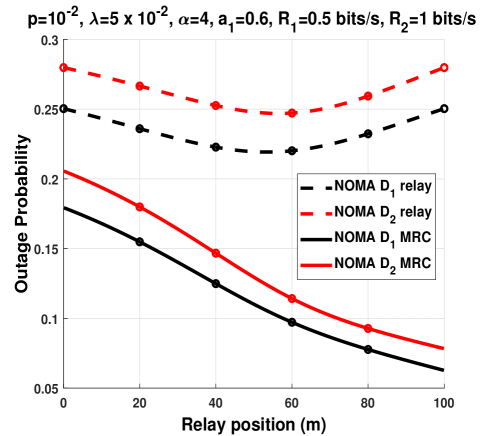
Figure 5: Outage probability as a function of the relay position, using a relay transmission and MRC transmission considering NOMA.

VI Conclusion

In this paper, we studied the improvement of using MRC in cooperative VCs transmission schemes considering NOMA at intersections. Closed form outage probability expressions were obtained. We compared the performance of MRC cooperative NOMA with a classical cooperative NOMA, and showed that MRC in cooperative NOMA transmission offers a significant improvement over the classical cooperative NOMA in terms of outage probability. We also compared the performance of MRC cooperative NOMA with MRC cooperative orthogonal multiple access (OMA), and we showed that NOMA has a better performance than OMA. Finally, we showed that the outage probability increases when the nodes come closer to the intersection, and that using MRC considering NOMA improves the performance in this context.

Appendix A

The outage probability related to $D_{1}$, denoted $\mathbb{P}(\textit{O}_{(1)})$, is expressed as

$$\mathbb{P}(\textit{O}_{(1)})=\mathbb{P}\Big{(}\mathcal{B}_{D_{1}}\cap\mathcal{A}_{D_{1}}\Big{)}+\mathbb{P}\Big{(}\mathcal{A}_{D_{1}}^{C}\cap\mathcal{C}_{D_{1}}\Big{)}$$ (23)

First, we calculate the probability $\mathbb{P}\Big{(}\mathcal{A}_{R_{1}}^{C}\cap\mathcal{C}_{D_{1}}\Big{)}$ as

$$\mathbb{P}\Big{(}\mathcal{A}_{R_{1}}^{C}\cap\mathcal{C}_{D_{1}}\Big{)} = \mathbb{E}_{I_{X},I_{Y}}\Bigg{[}\mathbb{P}\Bigg{\{}\ \frac{|h_{SR}|^{2}l_{SR}a_{1}}{|h_{SR}|^{2}l_{SR}a_{2}+I_{X_{R}}+I_{Y_{R}}}\geq\Theta_{1}$$

$$\bigcap\frac{\left(|h_{SD_{1}}|^{2}l_{SD_{1}}+|h_{RD_{1}}|^{2}l_{RD_{1}}\right)\,a_{1}}{\left(|h_{SD_{1}}|^{2}l_{SD_{1}}+|h_{RD_{1}}|^{2}l_{RD_{1}}\right)\,a_{2}+I_{X_{D_{1}}}+I_{Y_{D_{1}}}}<\Theta_{1}\Bigg{\}}\Bigg{]}$$

$$= \mathbb{E}_{I_{X},I_{Y}}\Bigg{[}\mathbb{P}\Bigg{\{}\ |h_{SR}|^{2}l_{SR}(a_{1}-\Theta_{1}a_{2})\geq\Theta_{1}\big{[}I_{X_{R}}+I_{Y_{R}}\big{]}$$

$$\bigcap\left(|h_{SD_{1}}|^{2}l_{SD_{1}}+|h_{RD_{1}}|^{2}l_{RD_{1}}\right)\,(a_{1}-\Theta_{1}a_{2})<\Theta_{1}\big{[}I_{X_{D_{1}}}+I_{Y_{D_{1}}}\big{]}\Bigg{\}}\Bigg{]}.$$

When $\Theta_{1}<a_{1}/a_{2}$, and setting $G_{1}=\Theta_{1}/(a_{1}-\Theta_{1}a_{2})$, we obtain

$$\mathbb{P}\Big{(}\mathcal{A}_{R_{1}}^{C}\cap\mathcal{C}_{D_{1}}\Big{)} = \mathbb{E}_{I_{X},I_{Y}}\Bigg{[}\mathbb{P}\Bigg{\{}\ |h_{SR}|^{2}\geq\frac{G_{1}}{l_{SR}}\big{[}I_{X_{R}}+I_{Y_{R}}\big{]}\Bigg{\}}$$ (26)

$$\times\Bigg{\{}1-\mathbb{P}\left(|h_{SD_{1}}|^{2}l_{SD_{1}}+|h_{RD_{1}}|^{2}l_{RD_{1}}\geq G_{1}\big{[}I_{X_{D_{1}}}+I_{Y_{D_{1}}}\big{]}\right)\Bigg{\}}\Bigg{]}.$$

Since $|h_{SR}|^{2}$ follows an exponential distribution with unit mean, and the second probability in (26) can be written as

$$\mathbb{P}\big{[}|h_{SD_{1}}|^{2}l_{SD_{1}}+|h_{RD_{1}}|^{2}l_{RD_{1}}\geq G_{1}(I_{X_{D_{1}}}+I_{Y_{D_{1}}})\big{]}=\\ \dfrac{l_{RD_{1}}\exp\Big{[}-\dfrac{G_{1}}{l_{RD_{1}}}(I_{X_{D_{1}}}+I_{Y_{D_{1}}})\Big{]}-l_{SD_{1}}\exp\Big{(}-\dfrac{G_{1}}{l_{SD_{1}}}[I_{X_{D_{1}}}+I_{Y_{D_{1}}})\Big{]}}{l_{RD_{1}}-l_{SD_{1}}}.$$ (27)

Then, the equation (26) becomes

$$\mathbb{P}\Big{(}\mathcal{A}_{R_{1}}^{C}\cap\mathcal{C}_{D_{1}}\Big{)}=\mathbb{E}_{I_{X},I_{Y}}\Bigg{[}\exp\left(\frac{G_{1}}{l_{SR}}\big{[}I_{X_{R}}+I_{Y_{R}}\big{]}\right)\\ \times 1-\dfrac{l_{RD_{1}}\exp\Big{[}-\dfrac{G_{1}}{l_{RD_{1}}}(I_{X_{D_{1}}}+I_{Y_{D_{1}}})\Big{]}-l_{SD_{1}}\exp\Big{(}-\dfrac{G_{1}}{l_{SD_{1}}}[I_{X_{D_{1}}}+I_{Y_{D_{1}}})\Big{]}}{l_{RD_{1}}-l_{SD_{1}}}\big{]}\Bigg{\}}\Bigg{]}\\ =\mathbb{E}_{I_{X},I_{Y}}\Bigg{[}\exp\left(\frac{G_{1}}{l_{SR}}\big{[}I_{X_{R}}+I_{Y_{R}}\big{]}\right)-\exp\left(\frac{G_{1}}{l_{SR}}\big{[}I_{X_{R}}+I_{Y_{R}}\big{]}\right)\\ \times\dfrac{l_{RD_{1}}\exp\Big{[}-\dfrac{G_{1}}{l_{RD_{1}}}(I_{X_{D_{1}}}+I_{Y_{D_{1}}})\Big{]}-l_{SD_{1}}\exp\Big{(}-\dfrac{G_{1}}{l_{SD_{1}}}[I_{X_{D_{1}}}+I_{Y_{D_{1}}})\Big{]}}{l_{RD_{1}}-l_{SD_{1}}}\big{]}\Bigg{\}}\Bigg{]}.$$ (28)

Using the independence of the PPP on the road $X$ and $Y$, and given that $\mathbb{E}[e^{sI}]=\mathcal{L}_{I}(s)$, we finally get

$$\mathbb{P}\Big{(}\mathcal{A}_{R_{1}}^{C}\cap\mathcal{C}_{D_{1}}\Big{)}=\mathcal{L}_{I_{X_{R}}}\bigg{(}\frac{G_{1}}{l_{SR}}\bigg{)}\mathcal{L}_{I_{Y_{R}}}\bigg{(}\frac{G_{1}}{l_{SR}}\bigg{)}\\ -\mathcal{L}_{I_{X_{R}}}\bigg{(}\frac{G_{1}}{l_{SR}}\bigg{)}\mathcal{L}_{I_{Y_{R}}}\bigg{(}\frac{G_{1}}{l_{SR}}\bigg{)}\frac{l_{RD_{1}}\mathcal{L}_{I_{X_{D_{1}}}}\bigg{(}\frac{G_{1}}{l_{RD_{1}}}\bigg{)}\mathcal{L}_{I_{Y_{D_{1}}}}\bigg{(}\frac{G_{1}}{l_{RD_{1}}}\bigg{)}-l_{SD_{1}}\mathcal{L}_{I_{X_{D_{1}}}}\bigg{(}\frac{G_{1}}{l_{SD_{1}}}\bigg{)}\mathcal{L}_{I_{Y_{D_{1}}}}\bigg{(}\frac{G_{1}}{l_{SD_{1}}}\bigg{)}}{l_{RD_{1}}-l_{SD_{1}}}.$$ (29)

The probability $\mathbb{P}\Big{(}\mathcal{B}_{D_{1}}\cap\mathcal{A}_{D_{1}}\Big{)}$ can be expressed as

$$\mathbb{P}\Big{(}\mathcal{B}_{D_{1}}\cap\mathcal{A}_{D_{1}}\Big{)} = 1-\mathbb{P}\Big{(}\mathcal{B}_{D_{1}}^{C}\cup\mathcal{A}_{D_{1}}^{C}\Big{)}$$ (30)

$$= 1-\mathbb{P}\Big{(}\mathcal{B}_{D_{1}}^{C}\Big{)}-\mathbb{P}\Big{(}\mathcal{A}_{D_{1}}^{C}\Big{)}+\mathbb{P}\Big{(}\mathcal{B}_{D_{1}}^{C}\cap\mathcal{A}_{D_{1}}^{C}\Big{)}$$

The final expression can acquired following the same steps above.

The outage probability related to $D_{2}$, denoted $\mathbb{P}(\textit{O}_{(2)})$, is expressed as

$$\mathbb{P}(\textit{O}_{(2)}) = \mathbb{P}\left[\Bigg{\{}\bigcup_{i=1}^{2}\mathcal{B}_{D_{2-i}}(\Theta_{i})\Bigg{\}}\cap\Bigg{\{}\ \bigcup_{i=1}^{2}\mathcal{A}_{R_{i}}(\Theta_{i})\Bigg{\}}\right]$$ (31)

$$+\mathbb{P}\left[\Bigg{\{}\bigcap_{i=1}^{2}\mathcal{A}_{R_{i}}^{C}(\Theta_{i})\Bigg{\}}\cap\Bigg{\{}\bigcup_{i=1}^{2}\mathcal{C}_{D_{2-i}}(\Theta_{i})\Bigg{\}}\right].$$

To calculate the first probability in (31), we proceed as follows

$$\mathbb{P}\left[\Bigg{\{}\bigcup_{i=1}^{2}\mathcal{B}_{D_{2-i}}(\Theta_{i})\Bigg{\}}\cap\Bigg{\{}\bigcup_{i=1}^{2}\mathcal{A}_{R_{i}}(\Theta_{i})\Bigg{\}}\right] = 1-\mathbb{P}\left[\Bigg{\{}\bigcap_{i=1}^{2}\mathcal{B}_{D_{2-i}}^{C}(\Theta_{i})\Bigg{\}}\cup\Bigg{\{}\bigcap_{i=1}^{2}\mathcal{A}_{R_{i}}^{C}(\Theta_{i})\Bigg{\}}\right]$$

$$= 1-\mathbb{P}\left[\bigcap_{i=1}^{2}\mathcal{B}_{D_{2-i}}^{C}(\Theta_{i})\right]-\mathbb{P}\left[\bigcap_{i=1}^{2}\mathcal{A}_{R_{i}}^{C}(\Theta_{i})\right]$$

$$+\mathbb{P}\left[\Bigg{\{}\bigcap_{i=1}^{2}\mathcal{B}_{D_{2-i}}^{C}(\Theta_{i})\Bigg{\}}\cap\Bigg{\{}\bigcap_{i=1}^{2}\mathcal{A}_{R_{i}}^{C}(\Theta_{i})\Bigg{\}}\right].$$

Since the computation of first and the second probability in (A) follow the same steps above, we only calculate the last probability in (A), hence, proceed as follows

$$\mathbb{P}\left[\Bigg{\{}\bigcap_{i=1}^{2}\mathcal{B}_{D_{2-i}}^{C}(\Theta_{i})\Bigg{\}}\cap\Bigg{\{}\bigcap_{i=1}^{2}\mathcal{A}_{R_{i}}^{C}(\Theta_{i})\Bigg{\}}\right]=\\ \mathbb{E}_{I_{X},I_{Y}}\Bigg{[}\mathbb{P}\Bigg{\{}\frac{|h_{SD_{2}}|^{2}l_{SD_{2}}a_{1}}{|h_{SD_{2}}|^{2}l_{SD_{2}}a_{2}+I_{X_{D_{2}}}+I_{Y_{D_{2}}}}\geq\Theta_{1},\frac{|h_{SD_{2}}|^{2}l_{SD_{2}}a_{2}}{I_{X_{D_{2}}}+I_{Y_{D_{2}}}}\geq\Theta_{2},\\ \frac{|h_{SR}|^{2}l_{SR}a_{1}}{|h_{SR}|^{2}l_{SR}a_{2}+I_{X_{R}}+I_{Y_{R}}}\geq\Theta_{1},\frac{|h_{SR}|^{2}l_{SR}a_{2}}{I_{X_{R}}+I_{Y_{R}}}\geq\Theta_{2}\Bigg{\}}\Bigg{]}.$$ (33)

When $\Theta_{1}<a_{1}/a_{2}$, and setting $G_{2}=\theta_{2}/a_{2}$, we obtain

$$\mathbb{P}\left[\Bigg{\{}\bigcap_{i=1}^{2}\mathcal{B}_{D_{2-i}}^{C}(\Theta_{i})\Bigg{\}}\cap\Bigg{\{}\bigcap_{i=1}^{2}\mathcal{A}_{R_{i}}^{C}(\Theta_{i})\Bigg{\}}\right]=\\ \mathbb{E}_{I_{X},I_{Y}}\Bigg{[}\mathbb{P}\Bigg{\{}|h_{SD_{2}}|^{2}\geq\frac{G_{1}}{l_{SD_{2}}}\big{[}I_{X_{D_{2}}}+I_{Y_{D_{2}}}\big{]},|h_{SD_{2}}|^{2}\geq\frac{G_{2}}{l_{SD_{2}}}\big{[}I_{X_{D_{2}}}+I_{Y_{D_{2}}}\big{]},\\ |h_{SR}|^{2}\geq\frac{G_{1}}{l_{SR}}\big{[}I_{X_{R}}+I_{Y_{R}}\big{]},|h_{SR}|^{2}\geq\frac{G_{2}}{l_{SR}}\big{[}I_{X_{R}}+I_{Y_{R}}\big{]}\Bigg{\}}\Bigg{]}\\ =\mathbb{E}_{I_{X},I_{Y}}\Bigg{[}\mathbb{P}\Bigg{\{}|h_{SD_{2}}|^{2}\geq\frac{\max(G_{1},G_{2})}{l_{SD_{2}}}\big{[}I_{X_{D_{2}}}+I_{Y_{D_{2}}}\big{]},|h_{SR}|^{2}\geq\frac{\max(G_{1},G_{2})}{l_{SR}}\big{[}I_{X_{R}}+I_{Y_{R}}\big{]}\Bigg{\}}\Bigg{]}.$$ (34)

Finally, we get

$$\mathbb{P}\left[\Bigg{\{}\bigcap_{i=1}^{2}\mathcal{B}_{D_{2-i}}^{C}(\Theta_{i})\Bigg{\}}\cap\Bigg{\{}\bigcap_{i=1}^{2}\mathcal{A}_{R_{i}}^{C}(\Theta_{i})\Bigg{\}}\right] = \mathcal{L}_{I_{X_{D_{2}}}}\bigg{(}\frac{G_{\mathrm{max}}}{l_{SD_{2}}}\bigg{)}\mathcal{L}_{I_{Y_{D_{2}}}}\bigg{(}\frac{G_{\mathrm{max}}}{l_{SD_{2}}}\bigg{)}$$ (35)

$$\times\>\mathcal{L}_{I_{X_{R}}}\bigg{(}\frac{G_{\mathrm{max}}}{l_{SR}}\bigg{)}\mathcal{L}_{I_{Y_{R}}}\bigg{(}\frac{G_{\mathrm{max}}}{l_{SR}}\bigg{)},$$

where $G_{\mathrm{max}}=\mathrm{max}(G_{1},G_{2})$.

Appendix B

The Laplace transform of the interference originating from the X road at $M$ is expressed as

$$\mathcal{L}_{{I_{X_{M}}}}(s)=\mathbb{E}\big{[}{\\ \exp(-sI_{X_{M}})}\big{]}.$$ (36)

Plugging (1) into (36) yields

$$\mathcal{L}_{{I_{X_{M}}}}(s) = \mathbb{E}\Bigg{[}{\exp\Bigg{(}-\sum_{x\in\Phi_{X_{M}}}s|h_{{M}x}|^{2}l_{{M}x}\Bigg{)}}\Bigg{]}$$ (37)

$$= \mathbb{E}\Bigg{[}\prod_{x\in\Phi_{X_{M}}}\exp\Bigg{(}-s|h_{{M}x}|^{2}l_{{M}x}\Bigg{)}\Bigg{]}$$

$$\overset{(a)}{=} \mathbb{E}\Bigg{[}\prod_{x\in\Phi_{X_{M}}}\mathbb{E}_{|h_{{M}x}|^{2},p}\Bigg{\{}\exp\Bigg{(}-s|h_{{M}x}|^{2}l_{Mx}\Bigg{)}\Bigg{\}}\Bigg{]}$$

$$\overset{(b)}{=} \mathbb{E}\Bigg{[}\prod_{x\in\Phi_{X_{M}}}\dfrac{p}{1+sl_{{M}x}}+1-p\Bigg{]}$$

$$\overset{(c)}{=} \exp\Bigg{(}-\lambda_{X}\displaystyle\int_{\mathbb{R}}\Bigg{[}1-\bigg{(}\dfrac{p}{1+sl_{{M}x}}+1-p\bigg{)}\Bigg{]}\textrm{d}x\Bigg{)}$$

$$= \exp\Bigg{(}-p\lambda_{X}\displaystyle\int_{\mathbb{R}}\dfrac{1}{1+1/sl_{{M}x}}\textrm{d}x\Bigg{)},$$

where (a) follows from the independence of the fading coefficients; (b) follows from performing the expectation over $|h_{{M}x}|^{2}$ which follows an exponential distribution with unit mean, and performing the expectation over the set of interferes; (c) follows from the probability generating functional (PGFL) of a PPP [30]. Then, substituting $l_{{M}x}=\|\textit{x}-M\|^{-\alpha}$ in (37) yields (17). The equation (19) can be acquired by following the same steps.

Appendix C

In order to calculate the Laplace transform of interference originated from the $X$ road at the node $M$, we have to calculate the integral in (17). We calculate the integral in (17) when $\alpha=2$. Let us take $m_{x}=m\cos(\theta_{M})$, and $m_{y}=m\sin(\theta_{M}$), then (17) becomes

$$\mathcal{L}_{I_{X_{M}}}(s) = \exp\Bigg{(}-\emph{p}\lambda_{X}\int_{\mathbb{R}}\dfrac{1}{1+m_{y}^{2}+(x-m_{x})^{2}/s}\textrm{d}x\Bigg{)}$$

$$= \exp\Bigg{(}-\emph{p}\lambda_{X}s\int_{\mathbb{R}}\dfrac{1}{s+m_{y}^{2}+(x-m_{x})^{2}}\textrm{d}x\Bigg{)}.$$

The integral inside the exponential in (C) equals

$$\int_{\mathbb{R}}\dfrac{1}{s+m_{y}^{2}+(x-m_{x})^{2}}\textrm{d}x=\dfrac{\pi}{\sqrt{m_{y}^{2}+s}}.$$ (39)

Then, plugging (39) into (C), we obtain

$$\mathcal{L}_{I_{X_{M}}}(s)=\exp\Bigg{(}-\emph{p}\lambda_{X}\dfrac{s\,\pi}{\sqrt{m_{y}^{2}+s}}\Bigg{)}.$$ (40)

Finally, substituting $m_{y}$ by $m\sin(\theta_{{M}})$ into (40) yields (21). Following the same steps above, and without details for the derivation, we obtain (22).

References

• [1] B. E. Y. Belmekki, A. Hamza, and B. Escrig, “Outage analysis of cooperative noma using maximum ratio combining at intersections,” in IEEE 15th Int. Conf. Wireless Mobile Comput. Netw. Commun. (WiMob), pp. 1–6, IEEE, 2019.
• [2] U.S. Dept. of Transportation, National Highway Traffic Safety Administration, “Traffic safety facts 2015,” Jan. 2017.
• [3] Z. Ding, Y. Liu, J. Choi, Q. Sun, M. Elkashlan, I. Chih-Lin, and H. V. Poor, “Application of non-orthogonal multiple access in lte and 5g networks,” IEEE Communications Magazine, vol. 55, no. 2, pp. 185–191, 2017.
• [4] Y. Saito, Y. Kishiyama, A. Benjebbour, T. Nakamura, A. Li, and K. Higuchi, “Non-orthogonal multiple access (noma) for cellular future radio access,” in Vehicular Technology Conference (VTC Spring), 2013 IEEE 77th, pp. 1–5, IEEE, 2013.
• [5] L. Dai, B. Wang, Y. Yuan, S. Han, I. Chih-Lin, and Z. Wang, “Non-orthogonal multiple access for 5g: solutions, challenges, opportunities, and future research trends,” IEEE Communications Magazine, vol. 53, no. 9, pp. 74–81, 2015.
• [6] S. R. Islam, N. Avazov, O. A. Dobre, and K.-S. Kwak, “Power-domain non-orthogonal multiple access (noma) in 5g systems: Potentials and challenges,” IEEE Communications Surveys & Tutorials, vol. 19, no. 2, pp. 721–742, 2017.
• [7] Z. Ding, Z. Yang, P. Fan, and H. V. Poor, “On the performance of non-orthogonal multiple access in 5g systems with randomly deployed users,” IEEE Signal Processing Letters, vol. 21, no. 12, pp. 1501–1505, 2014.
• [8] Z. Mobini, M. Mohammadi, H. A. Suraweera, and Z. Ding, “Full-duplex multi-antenna relay assisted cooperative non-orthogonal multiple access,” arXiv preprint arXiv:1708.03919, 2017.
• [9] K. S. Ali, H. ElSawy, A. Chaaban, M. Haenggi, and M.-S. Alouini, “Analyzing non-orthogonal multiple access (noma) in downlink poisson cellular networks,” in Proc. of IEEE International Conference on Communications (ICC18), 2018.
• [10] Z. Zhang, H. Sun, R. Q. Hu, and Y. Qian, “Stochastic geometry based performance study on 5g non-orthogonal multiple access scheme,” in Global Communications Conference (GLOBECOM), 2016 IEEE, pp. 1–6, IEEE, 2016.
• [11] H. Tabassum, E. Hossain, and J. Hossain, “Modeling and analysis of uplink non-orthogonal multiple access in large-scale cellular networks using poisson cluster processes,” IEEE Transactions on Communications, vol. 65, no. 8, pp. 3555–3570, 2017.
• [12] Y. Liu, Z. Qin, M. Elkashlan, A. Nallanathan, and J. A. McCann, “Non-orthogonal multiple access in large-scale heterogeneous networks,” IEEE Journal on Selected Areas in Communications, vol. 35, no. 12, pp. 2667–2680, 2017.
• [13] A. Tassi, M. Egan, R. J. Piechocki, and A. Nix, “Modeling and design of millimeter-wave networks for highway vehicular communication,” IEEE Transactions on Vehicular Technology, vol. 66, no. 12, pp. 10676–10691, 2017.
• [14] E. Steinmetz, M. Wildemeersch, T. Q. Quek, and H. Wymeersch, “A stochastic geometry model for vehicular communication near intersections,” in Globecom Workshops (GC Wkshps), 2015 IEEE, pp. 1–6, IEEE, 2015.
• [15] M. Abdulla, E. Steinmetz, and H. Wymeersch, “Vehicle-to-vehicle communications with urban intersection path loss models,” in Globecom Workshops (GC Wkshps), 2016 IEEE, pp. 1–6, IEEE, 2016.
• [16] J. P. Jeyaraj and M. Haenggi, “Reliability analysis of v2v communications on orthogonal street systems,” in GLOBECOM 2017-2017 IEEE Global Communications Conference, pp. 1–6, IEEE, 2017.
• [17] T. Kimura and H. Saito, “Theoretical interference analysis of inter-vehicular communication at intersection with power control,” Computer Communications, 2017.
• [18] B. E. Y. Belmekki, A. Hamza, and B. Escrig, “Cooperative vehicular communications at intersections over nakagami-m fading channels,” Vehicular Communications, p. doi:10.1016/j.vehcom.2019.100165, 07 2019.
• [19] B. E. Y. Belmekki, A. Hamza, and B. Escrig, “Performance analysis of cooperative communications at road intersections using stochastic geometry tools,” arXiv preprint arXiv:1807.08532, 2018.
• [20] B. E. Y. Belmekki, A. Hamza, and B. Escrig, “Outage performance of NOMA at road intersections using stochastic geometry,” in 2019 IEEE Wireless Communications and Networking Conference (WCNC) (IEEE WCNC 2019), pp. 1–6, IEEE, 2019.
• [21] B. E. Y. Belmekki, A. Hamza, and B. Escrig, “On the performance of 5g non-orthogonal multiple access for vehicular communications at road intersections,” Vehicular Communications, p. doi:10.1016/j.vehcom.2019.100202, 2019.
• [22] B. E. Y. Belmekki, A. Hamza, and B. Escrig, “On the outage probability of cooperative 5g noma at intersections,” in 2019 IEEE 89th Vehicular Technology Conference (VTC2019-Spring), pp. 1–6, IEEE, 2019.
• [23] B. E. Y. Belmekki, A. Hamza, and B. Escrig, “Performance analysis of cooperative noma at intersections for vehicular communications in the presence of interference,” Ad hoc Networks, p. doi:10.1016/j.adhoc.2019.102036, 2019.
• [24] B. E. Y. Belmekki, A. Hamza, and B. Escrig, “Non-orthogonal multiple access performance for millimeter wave in vehicular communications,” arXiv preprint arXiv:1909.12392, 2019.
• [25] B. E. Y. Belmekki, A. Hamza, and B. Escrig, “Outage analysis of cooperative noma in millimeter wave vehicular network at intersections,” arXiv preprint arXiv:1904.11022, 2019.
• [26] Z. Ding, M. Peng, and H. V. Poor, “Cooperative non-orthogonal multiple access in 5g systems,” IEEE Communications Letters, vol. 19, no. 8, pp. 1462–1465, 2015.
• [27] Z. Ding, H. Dai, and H. V. Poor, “Relay selection for cooperative noma,” IEEE Wireless Communications Letters, vol. 5, no. 4, pp. 416–419, 2016.
• [28] Z. Ding, L. Dai, and H. V. Poor, “Mimo-noma design for small packet transmission in the internet of things,” IEEE access, vol. 4, pp. 1393–1405, 2016.
• [29] M. O. Hasna, M.-S. Alouini, A. Bastami, and E. S. Ebbini, “Performance analysis of cellular mobile systems with successive co-channel interference cancellation,” IEEE Transactions on Wireless Communications, vol. 2, no. 1, pp. 29–40, 2003.
• [30] M. Haenggi, Stochastic geometry for wireless networks. Cambridge University Press, 2012.