The Scale Factor Potential Approach to Inflation

Abstract

We propose a new approach to investigate inflation in a model-independent way, and in particular to elaborate the involved observables, through the introduction of the “scale factor potential”. Through its use one can immediately determine the inflation end, which corresponds to its first (and global) minimum. Additionally, we express the inflationary observables in terms of its logarithm, using as independent variable the e-folding number. As an example, we construct a new class of scalar potentials that can lead to the desired spectral index and tensor-to-scalar ratio, namely $n_{s}\approx 0.965$ and $r\sim 10^{-4}$ for 60 $e$-folds, in agreement with observations.

I Introduction

The inflationary paradigm is considered as a necessary part of the standard model of cosmology, since it provides the solution to the fundamental puzzles of the old Big Bang theory, such as the horizon, the flatness, and the monopole problems Starobinsky (1979); Kazanas (1980); Starobinsky (1980); Guth (1981); Linde (1982); Albrecht and Steinhardt (1982); Barrow and Ottewill (1983); Blau et al. (1987). It can be achieved through various mechanisms, for instance through the introduction of primordial scalar field(s) Barrow and Paliathanasis (2016, 2018); Olive (1990); Linde (1994); Liddle et al. (1994); Lidsey et al. (1997); Cervantes-Cota and Dehnen (1995); Berera (1995); Armendariz-Picon et al. (1999); Kanti and Olive (1999); Garriga and Mukhanov (1999); Gordon et al. (2000); Bassett et al. (2006); Chen and Wang (2010); Germani and Kehagias (2010); Kobayashi et al. (2010); Feng et al. (2010); Burrage et al. (2011); Kobayashi et al. (2011); Ohashi and Tsujikawa (2012); Hossain et al. (2014); Wali Hossain et al. (2015); Cai et al. (2015); Geng et al. (2015); Kamali et al. (2016); Geng et al. (2017); Benisty and Guendelman (2018); Dalianis et al. (2019); Dalianis and Tringas (2019); Benisty et al. (2020); Benisty (2019); Benisty et al. (2019a, b); Staicova and Stoilov (2019a); Staicova (2019); Staicova and Stoilov (2019b); Guendelman (1999); Guendelman et al. (2015); Qiu et al. (2020), or through correction terms into the modified gravitational action Dvali and Tye (1999); Kawasaki et al. (2000); Bojowald (2002); Nojiri and Odintsov (2003); Kachru et al. (2003); Nojiri and Odintsov (2006); Ferraro and Fiorini (2007); Cognola et al. (2008); Cai and Saridakis (2011); Ashtekar and Sloan (2011); Qiu and Saridakis (2012); Briscese et al. (2013); Ellis et al. (2013); Basilakos et al. (2013); Sebastiani et al. (2014); Baumann and McAllister (2015); Dalianis and Farakos (2015); Kanti et al. (2015); De Laurentis et al. (2015); Basilakos et al. (2016); Bonanno and Platania (2015); Koshelev et al. (2016); Bamba et al. (2017); Motohashi and Starobinsky (2017); Oikonomou (2018); Benisty and Guendelman (2019); Antoniadis et al. (2018); Karam et al. (2019); Nojiri et al. (2019); Benisty et al. (2019c); Mukhanov (2013).

Additionally, inflation was proved crucial in providing a framework for the generation of primordial density perturbations Mukhanov and Chibisov (1981); Guth and Pi (1982). Since these perturbations affect the Cosmic Background Radiation (CMB), the inflationary effect on observations can be investigated through the prediction for the scalar spectral index of the curvature perturbations and its running, for the tensor spectral index, and for the tensor-to-scalar ratio.

The standard approach to calculate the above inflation related observables, is by performing a detailed perturbation analysis. Nevertheless, the procedure can be simplified if one imposes the slow-roll approximation and introduces the slow-roll parameters Martin et al. (2014), either in the case where inflation is driven by a scalar field and its potential, or in the case where inflation arises through gravitational modification.

In the present work we propose a new approach to investigate inflation, and in particular the involved observables, through the introduction of the “scale factor potential”. This scale factor potential is defined by demanding it to be opposite to the “kinetic energy” of the scale factor in order for them to add to zero. As we will see, it is very useful in studying inflation for every underlying theory, since through its use one can immediately determine the inflation end, namely at its minimum, as well as he can calculate the various inflationary observables.

The plan of the work is as follows: In section II we introduce the concept of the scale-factor potential. In section III we apply it in order to investigate inflation in general, and using it we propose a new inflationary scalar-field potential that can generate a spectral index and a tensor-to-scalar ratio in agreement with observations. Finally, in section V we summarize our results.

II Scale factor potential

In this section we introduce the concept of “scale factor potential”, which is a mathematical tool that proves very useful in performing inflationary calculations. We focus on the usual case of a homogeneous and isotropic cosmology with the Friedmann-Robertson-Walker (FRW) metric

$${\rm d}s^{2}=-{\rm d}t^{2}+a^{2}(t)\left[\frac{{\rm d}r^{2}}{1-Kr^{2}}+r^{2}\left(d\theta^{2}+\sin^{2}\theta d\phi^{2}\right)\right],$$ (1)

where $a(t)$ is the scale factor and $K$ determines spatial curvature, with value of $0$ for a spatially flat universe.

The scale factor potential $U(a)$ is defined by demanding it to opposite to the “kinetic energy” of the scale factor, i.e. $\dot{a}^{2}$, in order for them to add to zero, namely:

$$\dot{a}^{2}+U\left(a\right)=0,$$ (2)

and hence it has dimensions of inverse length square. In order to provide a more illustrating picture, let’s consider the general Friedmann equation in the case of $\Lambda$CDM paradigm, namely

$$H^{2}+\frac{K}{a^{2}}=\frac{8\pi G}{3}\left(\rho_{m}+\rho_{r}+\rho_{\Lambda}\right),$$ (3)

where $\rho_{m}$,$\rho_{r}$,$\rho_{\Lambda}$ correspond respectively to the energy density of matter, radiation and cosmological constant, and $G$ is the Newton’s constant. Hence, in this case the corresponding scale factor potential will be

$$U(a)=-a^{2}H_{0}^{2}\left[\Omega_{\Lambda}^{(0)}+\frac{\Omega_{K}^{(0)}}{a^{2}}+\frac{\Omega_{m}^{(0)}}{a^{3}}+\frac{\Omega_{r}^{(0)}}{a^{4}}\right],$$ (4)

where $\Omega_{i}^{(0)}$ are the values of the density parameters $\Omega_{i}=8\pi G\rho_{i}/3H^{2}$ at the present scale factor $a_{0}=1$, and $H_{0}$ is the present Hubble parameter (we have defined $\rho_{K}\equiv-3K/(8\pi Ga^{2})$). In Fig. 1 we depict $U(a)$ for the case where the Universe contains only the cosmological constant (de Sitter Universe), for the case of a matter-dominated Universe, and for the standard $\Lambda$CDM scenario.

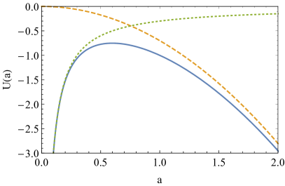
Figure 1: The scale factor potential $U(a)$ for the case of a flat de Sitter Universe (orange-dashed curve), i.e with $\Omega_{\Lambda}^{(0)}=1$, for the case of a flat matter-dominated universe (green-dotted curve), i.e with $\Omega_{m}^{(0)}=1$, and for $\Lambda$CDM paradigm (blue-solid curve), with $\Omega_{\Lambda}^{(0)}=0.7$, $\Omega_{m}^{(0)}=0.3$, in units where $H_{0}=1$.

III Application to Inflation

In this section we investigate the inflation realization using the scale factor potential introduced above. Let us first start by the description of the basic de Sitter evolution. One can immediately see that in such exponential expansion of the form $a(t)=a_{i}e^{H_{dS}(t-t_{i})}$ the scale factor potential (2) is just an inverse parabola, namely $U(a)=-H_{dS}^{2}a^{2}$, whose shape is determined by the de Sitter Hubble parameter value $H_{dS}$. Hence, we deduce that in any physically interesting inflationary scenario, the scale factor potential will start from an inverse parabola at small scale factors, and then as the universe proceeds towards the inflationary exit $U(a)$ will deviate accordingly.

The important issue in a successful inflationary realization is the calculation of various inflation-related observables, such as the scalar spectral index of the curvature perturbations $n_{\mathrm{s}}$, its running $\alpha_{\mathrm{s}}\equiv dn_{\mathrm{s}}/d\ln k$, where $k$ is the absolute value of the wave number $\vec{k}$, the tensor spectral index $n_{\mathrm{T}}$ and the tensor-to-scalar ratio $r$. These quantities are determined by observational data very accurately, and hence confrontation can constrain of exclude the studied scenarios.

In general, the calculation of the above observables demands a detailed perturbation analysis. Nevertheless, one can obtain approximate expressions by imposing the slow-roll assumptions, under which all inflationary information is encoded in the slow-roll parameters. In particular, one first introduces Martin et al. (2014)

$$\epsilon_{n+1}=\frac{d}{dN}\log|\epsilon_{n}|,$$ (5)

where $\epsilon_{0}\equiv H_{i}/H$ and $N\equiv\ln(a/a_{i})$ is the e-folding number, with $a_{i}$ the scale factor at the beginning of inflation, $H_{i}$ the corresponding Hubble parameter, and $n$ a positive integer. As usual inflation ends at a scale factor $a_{f}$ where $\ddot{a}=0$, i.e. where $\epsilon_{1}(a_{f})=1$, and the slow-roll approximation breaks down. Finally, in terms of the first three $\epsilon_{n}$, which are easily found to be

$$\!\!\!\!\!\!\!\!\!\!\!\!\!\!\epsilon_{1}\equiv-\frac{\dot{H}}{H^{2}},$$ (6)

$$\!\!\!\!\!\!\!\!\!\!\!\!\!\!\epsilon_{2}\equiv\frac{\ddot{H}}{H\dot{H}}-\frac{2\dot{H}}{H^{2}},$$ (7)

$$\!\!\!\!\!\!\!\!\!\!\!\!\!\!\epsilon_{3}\equiv\left(\ddot{H}H-2\dot{H}^{2}\right)^{-1}$$

$$\!\!\!\!\cdot\!\left[\frac{H\dot{H}\dddot{H}-\ddot{H}(\dot{H}^{2}+H\ddot{H})}{H\dot{H}}-\frac{2\dot{H}}{H^{2}}(H\ddot{H}-2\dot{H}^{2})\right]\!,$$ (8)

the inflationary observables are expressed as Martin et al. (2014)

$$r \approx 16\epsilon_{1},$$ (9)

$$n_{\mathrm{s}} \approx 1-2\epsilon_{1}-\epsilon_{2},$$ (10)

$$\alpha_{\mathrm{s}} \approx -2\epsilon_{1}\epsilon_{2}-\epsilon_{2}\epsilon_{3},$$ (11)

$$n_{\mathrm{T}} \approx -2\epsilon_{1},$$ (12)

where all quantities are calculated at $a_{i}$.

Let us now see how the above approach is simplified with the use of the scale factor potential $U(a)$. In particular, using the definition (2) we can immediately express the slow-roll parameters above as:

$$\!\!\!\!\!\!\!\!\!\!\!\epsilon_{1}=1-\frac{aU^{\prime}}{2U},$$ (13)

$$\!\!\!\!\!\!\!\!\!\!\!\epsilon_{2}=\frac{a\left\{aU^{\prime 2}-U\left[aU^{\prime\prime}+U^{\prime}\right]\right\}}{U\left(2U-aU^{\prime}\right)},$$ (14)

$$\!\!\!\!\!\!\!\!\!\!\!\epsilon_{3}=\left\{U\left(2U-aU^{\prime}\right)\left[U\left(aU^{\prime\prime}+U^{\prime}\right)-aU^{\prime 2}\right]\right\}^{-1}$$

$$\ \cdot\Big{\{}-a^{3}U^{\prime 4}+a^{2}UU^{\prime 2}\left(aU^{\prime\prime}+5U^{\prime}\right)$$

$$\ \ \ \ \,-aU^{2}\left[-a^{2}U^{\prime\prime 2}+aU^{\prime}\left(aU^{\prime\prime\prime}+7U^{\prime\prime}\right)+6U^{\prime 2}\right]$$

$$\ \ \ \ \,+2U^{3}\left[a\left(aU^{\prime\prime\prime}+3U^{\prime\prime}\right)+U^{\prime}\right]\Big{\}},$$ (15)

where primes denote derivatives with respect to $a$. The end of inflation is obtained when $\epsilon_{1}(a_{f})=1$. Eq. (13) with $\epsilon_{1}=1$ yields $U^{\prime}(a_{f})=0$. Hence, we deduce that inflation ends at the minimum of the scale factor potential (we know that it is minimum and not a maximum since as we mentioned the evolution in every inflationary model starts close to de Sitter i.e. to the inverse parabola $U(a)=-H_{dS}^{2}a^{2}$, thus it starts from a maximum of $U(a)$. The simplicity of the condition $U^{\prime}(a_{f})=0$ reveals the advantage of the use of $U(a)$). This feature will become useful later on. Finally, by inserting relations (13)-(III) calculated at $a_{i}$ into (9)-(12) we obtain the inflationary observables.

Since the e-folding number is defined as the logarithm of the scale factor, namely $N\equiv\ln(a/a_{i})$, we can introduce the logarithm of the scale factor potential as

$$P=-\ln\left[\frac{U(a)}{U(a_{i})}\right].$$ (16)

Using these variables the Hubble function is expressed in terms of the e-folding number as

$$H(N)=H(0)\,\exp\left[-N-\frac{1}{2}P(N)\right],$$ (17)

which proves to be very useful since it is straightforwardly relates $H$ with $N$, i.e. to the variable which determines the duration of a successful inflation (a successful inflation needs $\mathcal{N}_{f}\sim 50-70$). Finally, inserting these variables into (13)-(III) we express the slow-roll parameters is a simple way as (5):

$$\epsilon_{1}=1+\frac{1}{2}P^{\prime}\left(N\right),$$ (18)

$$\epsilon_{2}=\frac{P^{\prime\prime}\left(N\right)}{P^{\prime}\left(N\right)+2},$$ (19)

$$\epsilon_{3}=\frac{P^{\prime\prime\prime}(N)}{P^{\prime\prime}(N)}-\frac{P^{\prime\prime}\left(N\right)}{P^{\prime}\left(N\right)+2}.$$ (20)

Since inflation ends when $\epsilon_{1}(\mathcal{N}_{f})=1$, from (18) we deduce that this happens at $P^{\prime}(\mathcal{N}_{f})=0$, i.e at the minimum of $P$, which was expected since as we mentioned above inflation ends at the minimum of $U$.

Inserting relations (18)-(20) calculated at the beginning of inflation, i.e. at $N=0$, into (9)-(12) we obtain the inflationary observables. In particular, doing so we find:

$$r\approx 16+8P^{\prime}\left(0\right),$$ (21)

$$n_{\mathrm{s}}\approx-1-P^{\prime}\left(0\right)-\frac{P^{\prime\prime}\left(0\right)}{P^{\prime}\left(0\right)+2},$$ (22)

$$\alpha_{\mathrm{s}}\approx-P^{\prime\prime}(0)-\frac{P^{\prime\prime\prime}(0)}{P^{\prime}(0)+2}+\left[\frac{P^{\prime\prime}(0)}{P^{\prime}(0)+2}\right]^{2},$$ (23)

$$n_{\mathrm{T}}\approx-2-P^{\prime}\left(0\right).$$ (24)

Hence, as we can see, the initial values for $P$ and its derivatives, i.e. of the scale factor potential and its derivatives, are the crucial ones in determining the value of the inflationary observables. In the slow-roll approximation in the beginning of inflation we have $\epsilon_{n}\ll 1$, which using expressions (18)-(20) lead to

$$-2\lesssim P^{\prime}\left(0\right)\ll 0$$

$$0\lesssim P^{\prime\prime}(0)\ll P^{\prime}(0)+2.$$ (25)

We proceed by exploring the properties of the logarithm of the scale factor potential $P(N)$ in order to obtain inflationary observables, and in particular spectral index $n_{\mathrm{s}}$ and tensor-to-scalar ratio $r$, in agreement with observations. From (21),(22) we acquire

$$P^{\prime}(0)=\frac{r}{8}-2$$ (26)

$$P^{\prime\prime}(0)=\frac{r}{64}\left[8(1-n_{\mathrm{s}})-r\right].$$ (27)

Hence, we need to introduce a parametrization for $P(N)$ that could incorporate these. From the definition (17) we find that the pure de Sitter solution gives $P_{dS}=-2N$, and thus $P_{dS}(0)=0$, $P_{dS}^{\prime}(0)=-2$, $P_{dS}^{\prime\prime}(0)=0$, which corresponds to the inverse parabola behavior of the scale factor potential mentioned above. Since the bulk of inflation corresponds to an exponential expansion, a good parametrization for $P(N)$ should be a suitable deviation from this de Sitter form.

The above scale factor potential formalism is of general applicability in any inflation realization, whether this is driven by a scalar field, or it arises effectively from modified gravity, or from any other mechanism. In order to provide a more transparent picture let us consider as an example the well-known Starobinsky inflation Starobinsky (1979); Barrow and Ottewill (1983); Barrow and Cotsakis (1988); Barrow (1988). This scenario arises from a quadratic $f(R)$ gravity of the form $f(R)=\frac{1}{16\pi G}R+\frac{1}{2M^{2}}R^{2}$, with $M$ a mass scale, which transformed in the Einstein frame is equivalent with a canonical scalar field $\phi$ moving in a potential Barrow and Cotsakis (1988); Barrow (1988):

$$V\left(\phi\right)=\frac{M^{2}}{32\pi G}\left(1-e^{-\sqrt{16\pi G/3}\phi}\right)^{2}.$$ (28)

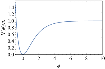
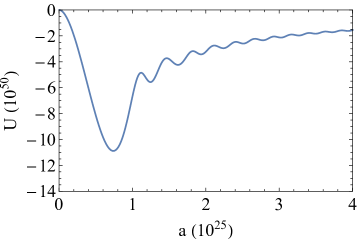
Figure 2: Upper graph: The scalar field potential $V(\phi)$ in the Einstein frame of the Starobinsky inflation. Lower graph: The corresponding scale factor potential $U(a)$ as it is numerically reconstructed from the solution of Eqs. (28)-(31). Inflation ends at the global minimum of $U(a)$, and its subsequent oscillations correspond to the scalar oscillations around the minimum of $V(\phi)$ during the reheating phase. We use units where $8\pi G=1$ and we set the scale factor at the beginning of inflation to $a_{i}=1$.

The Friedmann equations are:

$$H^{2}=\frac{8\pi G}{3}\left[\frac{1}{2}\dot{\phi}^{2}+V(\phi)\right],$$ (30)

$$\dot{H}=-4\pi G\dot{\phi}^{2},$$

while the Klein Gordon equation for the scalar field is

$$\ddot{\phi}+3H\dot{\phi}+V^{\prime}(\phi)=0.$$ (31)

In the upper panel of Fig. 2 we present the shape of the Starobinsky potential (28). On the lower panel we depict the corresponding scale factor potential as it is numerically reconstructed from the evolution of Eqs. (28)-(31). As we observe, and as analyzed in detail above, the scale factor potential starts with an inverse parabola at the initial scale factors and inflation durates up to its first (and global) minimum. The subsequent oscillations of $U(a)$ correspond to the scalar oscillations around the minimum of the physical potential $V(\phi)$ during the reheating phase Kofman et al. (1997). Note the advantage that in the scale factor potential picture we know exactly the inflation end, namely at its minimum, while in the usual potential picture it is not straightforwardly determined when the slow roll finishes and inflation ends.

IV Parameterization of the Potential

In this section we consider a specific example of the above formalism. We apply the parametrization

$$P(N)=-2\left(\frac{1}{N_{0}+N}+N\right),$$ (32)

with $N_{0}$ the model parameter. This form satisfies the condition (25). Using that the end of inflation happens at $P^{\prime}(\mathcal{N}_{f})=0$ it gives:

$$N_{f}+N_{0}=1.$$ (33)

The corresponding slow-roll parameters (18)-(20) read:

$$\epsilon_{1}=\frac{1}{(N_{0}+N)^{2}}$$

$$\epsilon_{2}=-\frac{2}{N_{0}+N}$$

$$\epsilon_{3}=-\frac{1}{N_{0}+N}.$$ (34)

Moreover, all other slow-roll parameters are the same with $\epsilon_{3}$. As we can see, the advantage of the ansatz (32) is that all slow-roll parameters are small and therefore the initial state is by construction close to de Sitter solution. The inflationary observables become

$$r=\frac{16}{(\mathcal{N}_{f}-1)^{2}}$$ (35)

$$n_{s}=\frac{(\mathcal{N}_{f}-4)\mathcal{N}_{f}+1}{(\mathcal{N}_{f}-1)^{2}}.$$ (36)

Taking as an example the e-folding number as $\mathcal{N}_{f}=60$ we find that

$$r=0.00459,\quad n_{\mathrm{s}}=0.9655.$$ (37)

Eliminating $\mathcal{N}_{f}$ between (35)-(36) gives

$$r=-8\left(n_{\mathrm{s}}-2+\sqrt{3-2n_{\mathrm{s}}}\right),$$ (38)

which is a very useful expression since it allows for a direct comparison with observations.

Figure 3: 1$\sigma$ (magenta) and 2$\sigma$ (light magenta) contours for Planck 2018 results (Planck $+TT+lowP$) Akrami et al. (2018), on $n_{\mathrm{s}}-r$ plane. Additionally, we present the predictions of the scale factor potential (32) with $50\leq\mathcal{N}_{f}\leq 70$, according to (38) ($n_{\mathrm{s}}=0.9584$ for $\mathcal{N}_{f}=50$ and $n_{\mathrm{s}}=0.9706$ for $\mathcal{N}_{f}=70$).

In Fig. 3 we present the predictions of the scenario at hand in the $n_{s}-r$ plane, for e-folding numbers $\mathcal{N}_{f}$ varying between 50 and 70, on top of the 1$\sigma$ and 2$\sigma$ likelihood contours of the Planck 2018 results Akrami et al. (2018); Aghanim et al. (2018). As we can see, the agreement with observations is very efficient, and the predictions lie well within the 1$\sigma$ region. Moreover, in the future Euclid and SPHEREx missions and the BICEP3 experiment, are expected to provide better observational bounds to test these predictions.

We can now proceed in applying the scale factor potential approach in order to reconstruct a physical scalar-field potential that can generate the desirable inflationary observables. From the definition of the scale factor potential (2), as well as the Friedmann equation (30) that holds in every scalar-field inflation, we extract the following solutions:

$$\phi(a)=-\int_{a_{i}}^{a}\frac{\sqrt{2U(a)-aU^{\prime}(a)}}{a\sqrt{U(a)}}\,da,$$ (39)

$$V(\phi(a))=V_{0}-\frac{a\,U^{\prime}(a)+4U(a)}{2a^{2}}.$$ (40)

Expressed in terms of the e-folding number $N$ and the logarithm of the scale factor potential $P(N)$ of (16) the above solutions become:

$$\phi(N)=-\int_{0}^{N}\sqrt{2+P^{\prime}(N)}\,dN,$$ (41)

$$V(\phi(N))=V_{0}+e^{-P(N)-2N}\left[2-\frac{1}{2}P^{\prime}(N)\right].$$ (42)

Let us apply the above formalism in our specific parametrization (32). Inserting it into (41)-(42) finally yields:

$$\!\!\!\!\!\!\!\!\!\!\!\!\!\!\!\!\phi(N)=\sqrt{2}\log\left(\frac{N+N_{0}}{N_{0}}\right)$$ (43)

and

$$\begin{split}V(\phi(N))=H_{0}^{2}e^{\frac{2}{N_{0}+N}}\left[3-\frac{1}{(N_{0}+N)^{2}}\right].\end{split}$$ (44)

Expression (43) can be inversed, in order to find $N(\phi)$ and then through insertion into (44) to extract $V(\phi)$ analytically as

$$\!\!\!\!\!\!\!\!\!\!\!\!\!\!\!\!V(\phi)=H_{0}^{2}e^{\frac{2e^{-\frac{\phi}{\sqrt{2}}}}{N_{0}}-\sqrt{2}\phi}\left(3N_{0}^{2}e^{\sqrt{2}\phi}-1\right).$$ (45)

Hence, this potential is the physical potential that leads to the observables depicted in Fig. 3. In Fig. 4 we depict the scale factor potential $U(a)$ of the parameterization (32), as well as the corresponding scalar-field potential $V(\phi)$ of (45). The universe begins with $\phi\gg 1$ with a slow-roll behavior, and the scalar field moves towards the left. The asymptotic values of the potential are:

$$V_{+\infty}=3H^{2}_{0},\quad V_{-\infty}=0,$$ (46)

and thus $3H^{2}_{0}$ represents the energy scale of the inflationary epoch.

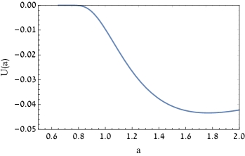
Figure 4: Upper graph: The scale factor potential $U(a)$ of the parameterization (32). Lower graph: The corresponding scalar-field potential $V(\phi)$ of (45), normalized by its value at $\infty$. We use units where $8\pi G=1$ and we set the scale factor at the beginning of inflation to $a_{i}=1$. We consider e-folding number $\mathcal{N}_{f}=60$, and thus (33) gives $N_{0}=-59$. Inflation ends at the global minimum of $U(a)$.

We close this section by mentioning that the above potential reconstruction was just an example that arose from the consideration of the polynomial parametrization of $P(N)$ in (32). By imposing other parametrizations we can obtain, numerically or analytically, other potential forms that lead to the desired inflationary observables. Such capabilities reveal the advantages of the approach at hand.

V Conclusions

In this work we proposed a new approach to investigate inflation in a model-independent way, and in particular to elaborate the involved observables, through the introduction of the “scale factor potential” $U(a)$ . This potential is defined by demanding it to be opposite to the “kinetic energy” of the scale factor in order for them to add to zero.

The scale factor potential is very useful in studying inflation for every underlying theory. Firstly, through its use one can immediately determine the inflation end, which corresponds to its first (and global) minimum, which is an advantage comparing to the usual potential picture, in which it is not straightforwardly determined when the slow roll finishes and inflation ends. The subsequent oscillations of $U(a)$ correspond to the scalar oscillations around the minimum of the physical potential during the reheating phase.

Additionally, we expressed the inflationary observables, such as the spectral index and its running, the tensor-to-scalar ratio, and the tensor spectral index, in terms of the scale factor potential and its derivatives. Then we introduced the logarithm $P$ of $U$ and we used as independent variable the e-folding number $N$, re-expressing the inflationary observables straightaway in terms of the initial values of $P$ and its derivatives. In this way, introducing parametrizations for $P(N)$ we were able to reconstruct $U$ that leads to the imposed inflationary observables.

We applied it in order to reconstruct a physical scalar-field potential that can generate the desirable inflationary observables. Hence, as an example, we reconstructed analytically a new class of scalar-potentials that can lead to the desired spectral index and tensor-to-scalar ratio, in agreement with observations.

Finally, by imposing other parametrizations for $P(N)$ we can obtain, numerically or analytically, other potential forms that lead to the given inflationary observables. Such capabilities reveal the advantages of the use of the scale factor potential.