Using Weaker Consistency Models with Monitoring and Recovery for Improving Performance of Key-Value Stores

Abstract

Consistency properties provided by most key-value stores can be classified into sequential consistency and eventual consistency. The former is easier to program with but suffers from lower performance whereas the latter suffers from potential anomalies while providing higher performance. We focus on the problem of what a designer should do if he/she has an algorithm that works correctly with sequential consistency but is faced with an underlying key-value store that provides a weaker (e.g., eventual or causal) consistency. We propose a detect-rollback based approach: The designer identifies a correctness predicate, say $P$, and continues to run the protocol, as our system monitors $P$. If $P$ is violated (because the underlying key-value store provides a weaker consistency), the system rolls back and resumes the computation at a state where $P$ holds.

We evaluate this approach with graph-based applications running on the Voldemort key-value store. Our experiments with deployment on Amazon AWS EC2 instances shows that using eventual consistency with monitoring can provide a $50\%$ – $80\%$ increase in throughput when compared with sequential consistency. We also observe that the overhead of the monitoring itself was low (typically less than $4\%$) and the latency of detecting violations was small. In particular, in a scenario designed to intentionally cause a large number of violations, more than $99.9\%$ of violations were detected in less than $50\text{\,}\mathrm{m}\mathrm{i}\mathrm{l}\mathrm{l}\mathrm{i}\mathrm{s}\mathrm{e}\mathrm{c}\mathrm{o}\mathrm{n}\mathrm{d}\mathrm{s}$ in regional networks (all clients and servers in the same Amazon AWS region), and in less than $3\text{\,}\mathrm{s}\mathrm{e}\mathrm{c}\mathrm{o}\mathrm{n}\mathrm{d}\mathrm{s}$ in global networks.

We find that for some applications, frequent rollback can cause the program using eventual consistency to effectively stall. We propose alternate mechanisms for dealing with re-occurring rollbacks. Overall, for applications considered in this paper, we find that even with rollback, eventual consistency provides better performance than using sequential consistency.

Research

1 Introduction

Distributed key-value data stores have gained increasing popularity due to their simple data model and high performance [1]. A distributed key-value data store, according to CAP theorem [2, 3], cannot simultaneously achieve sequential consistency and availability while tolerating network partitions. Since fault-tolerance, especially the provision of an acceptable level of service in the presence of node or channel failures, is a critical dependability requirement of any system, network partition tolerance is a necessity. Hence, it is inevitable to make trade-offs between availability and consistency, resulting in a spectrum of weaker consistency models such as causal consistency and eventual consistency [4, 5, 6, 1, 7, 8, 9].

Weaker consistency models are attractive because they have the potential to provide higher throughput and higher customer satisfaction. On the other hand, weaker consistency models suffer from data conflicts. Although such data conflicts are infrequent [1], such incidences will affect the correctness of the computation and invalidate subsequent results.

Furthermore, developing algorithms for the sequential consistency model is easier than developing those for weaker consistency models. Moreover, since the sequential consistency model is more natural, the designer may already have access to an algorithm that is correct only under sequential consistency. Thus, in this case, the question for the designer is what to do if the underlying system provides a weaker consistency or if the underlying system provides better performance under weaker consistency models?

As an illustration of such a scenario, consider a distributed computation that relies on a key-value store to arrange exclusive access to a critical resource for the clients. If the key-value store employs sequential consistency and the clients use Peterson’s algorithm, mutual exclusion is guaranteed [10], but the performance would be impeded due to the strict requirement of sequential consistency. If eventual consistency is adopted, then mutual exclusion is violated.

In this case, the designer has two options: (1) Either develop a brand new algorithm that works under eventual consistency, or (2) Run the algorithm by pretending that the underlying system satisfies sequential consistency but monitor it to detect violations of the mutual exclusion requirement. In case of the first option, we potentially need to develop a new algorithm for every consistency model used in practice, whereas in case of the second option, the underlying consistency model is irrelevant although we may need to rollback the system to an earlier state if a violation is found. While the rollback in general distributed systems is a challenging task, existing approaches have provided rollback mechanisms for key-value stores with low overhead [11]. Moreover, it is possible to develop efficient application-specific rollback algorithms by exploiting the properties of applications.

The predicate $P$ to monitor depends on the application. For the mutual exclusion application we alluded to above, $P$ might be exclusive access to the shared resource. As another example, consider the following. For many distributed graph processing applications, the clients process a given set of graph nodes. Since the state of a node depends on its neighbors, the clients need to coordinate to avoid updating two neighboring nodes simultaneously, otherwise they may read inconsistent information. In this case, predicate $P$ is the conjunction of smaller predicates and each smaller predicate proscribes the concurrent access to one pair of neighboring graph nodes (Note that pairs of neighboring nodes belonging to the same client do not need monitoring). We note that in a general problem, a smaller predicate may involve any number of processes. The application will continue executing as long as predicate $P$ is true. If $P$ is violated, the system will be rolled back to an earlier correct state from where subsequent execution will resume (cf. Figure 1).

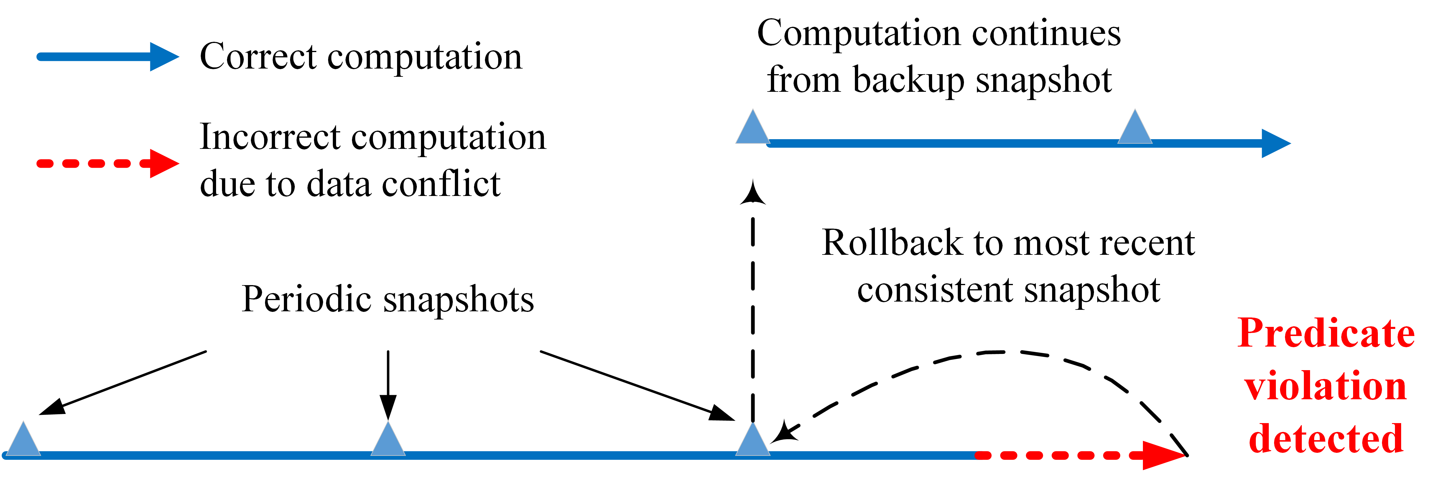
Figure 1: The detect-rollback approach: when the predicate of interest is violated, system state is restored to the most recent consistent snapshot and the computation resumes from there.

We require that the monitoring module is non-intrusive, i.e., it allows the underlying system to execute unimpeded. To evaluate the effectiveness of the monitors, we need to identify three parameters: (1) The benefit of using the monitors instead of relying on sequential consistency, (2) The overhead of the monitors, i.e., how the performance is affected when we introduce the monitoring module, and (3) Detection latency of the monitors, i.e., how long the monitors take to detect violation of $P$. (Note that since the monitoring module is non-intrusive, it cannot prevent violation of $P$.)

Contributions of the paper. We implement the monitors for linear and semilinear predicates based on the algorithms in [12, 13, 14] and develop a rollback algorithm for some graph-based applications. We integrate our prototype into LinkedIn’s Voldemort key-value store and run experiments on Amazon AWS network. Besides Amazon AWS network, we also run experiments on our local lab network where we can control network condition such as network latency. We evaluate our approach by running graph-based applications motivated by the task of Social Media Analysis on social graphs and Weather Monitoring on planar graphs. The source code and experiment results are available at [15]. The observations from the experiments are as follows:

• On Amazon AWS network, we run both sequential consistency without the monitors and eventual consistency with the monitors. We observe that –even with the overhead of the monitors– eventual consistency achieves a higher throughput than sequential consistency does. Specifically, the aggregate client throughput was improved by $50\%$ – $80\%$ when running Social Media Analysis motivated applications, and by $37\text{\,}\mathrm{\char 37\relax}$ on Weather Monitoring motivated applications. Furthermore, in those experiments, we find that violation of mutual exclusion is not frequent. For example, on Social Media Analysis, a violation occurred every $4,500\text{\,}\mathrm{s}$ on average, and was detected within $3\text{\,}\mathrm{s}$.

• We also evaluate the overhead of the monitoring module if it is intended solely for debugging or runtime monitoring. We find that when the monitors were used with sequential consistency, the overhead was at most $8\text{\,}\mathrm{\char 37\relax}$. And, for eventual consistency, the overhead was less than $4\text{\,}\mathrm{\char 37\relax}$.

• We design test cases with a large number of violations to stress the monitors. In those test cases, more than $99.9\text{\,}\mathrm{\char 37\relax}$ of violations were detected within $50\text{\,}\mathrm{ms}$ for Amazon AWS regional network (all machines in the same region), and within $3\text{\,}\mathrm{s}$ for the global network (machines in multiple regions).

• To evaluate the final benefit the applications can achieve after accounting for the cost of the monitors and rollback, we run graph-based applications with our rollback algorithm on the local lab network. We observe the final benefit varies depending on the properties of applications. Specifically, on non-terminating applications such as Weather Monitoring, the progress of the application running on eventual consistency with monitors and rollback was $45\%$ – $47\%$ faster than running on sequential consistency. On the other hand, on terminating applications such as Social Media Analysis, the final application progress benefit was $10\%$ – $20\%$. One of the reasons for the reduced benefit in terminating applications is that at the end of terminating execution, there are a few nodes to be processed, thus the chance of conflicts and recurring violations is increased during this time. In fact, if the application keeps using eventual consistency, the computation may stall due to repeated rollbacks (livelocks). We use some strategies such as backoff and adaptive consistency to handle the livelock issue. We also observe that terminating applications using our approach progressed $16\%$ – $28\%$ faster than using sequential consistency during the first $90\text{\,}\mathrm{\char 37\relax}$ of the work, and $10\%$ – $20\%$ faster overall (because it has to switch from eventual consistency to sequential consistency during the end of the execution).

To the best of our knowledge, our work is the first to experimentally quantify and analyze the benefits of eventual consistency with monitoring and rollback (compared to sequential consistency) on key-value stores. We also propose an efficient rollback algorithm for graph-based applications. Our results suggest that several correctness-sensitive applications are able to take advantage of weaker consistency models from the underlying data store to improve their performance while still preserving the correctness/safety properties. This opens an alternate design option and gives more flexibility to the application designer.

Organization of the paper: Section 2 describes the architecture of the key-value store used in this paper. In section 3, we define the notion of causality and identify how the uncertainty of event ordering in distributed systems affects the problem of predicate detection. Section 4 describes the overall architecture of the system using monitors. Section 5 explains the design of the predicate detection module used in this paper. In section 6, we discuss rollback approaches when a violation is detected, and develop a rollback algorithm for some graph-based applications. Section 7 presents experimental results and discussion. Section 8 compares our paper with related work and we conclude the paper in Section 9.

2 System Architecture

2.1 Distributed Key-Value Store

We utilize the standard architecture for key-value stores. Specifically, the data consists of (one or more) tables with two fields, a unique key and the corresponding value. The field value consists of a list of $<version,value>$ pairs. A version is a vector clock that describes the origin of the associated value. It is possible that a key has multiple versions when different clients issue PUT (write) requests for that key independently. When a client issues a GET (read) request for a key, all existing versions of that key will be returned. The client could resolve multiple versions for the same key on its own or use the resolver function provided from the library. To provide efficient access to this table, it is divided into multiple partitions. Furthermore, to provide redundancy and ease of access, the table is replicated across multiple replicas.

To access the entries in this table, the client utilizes two operations, GET and PUT. The operation GET($x$) provides the client with the value (or values if multiple versions exist) associated with key $x$. The operation PUT($x,val$) changes the value associated with key $x$ to $val$. The state of the servers can be changed only by PUT requests from clients.

2.2 Voldemort Key Store

Voldemort is LinkedIn’s open source equivalence of Amazon’s Dynamo key-value store. In Voldemort, clients are responsible for handling replication. When connecting to a server for the first time, a client receives meta-data from the server. The meta-data contains the list of servers and their addresses, the replication factor ($N$), required reads ($R$), required writes ($W$), and other configuration information.

When a client wants to perform a PUT (or GET) operation, it sends PUT (GET) requests to $N$ servers and waits for the responses for a predefined amount of time (timeout). If at least $W$ ($R$) acknowledgments (responses) are received before the timeout, the PUT (GET) operation is considered successful. If not, the client performs one more round of requests to other servers to get the necessary number of acknowledgments (responses). After the second round, if still less than $W$ ($R$) replies are received, the PUT (GET) operation is considered unsuccessful.

Since the clients do the task of replication, the values $N$, $R$, $W$ specified in the meta-data is only a suggestion. The clients can change those values for their needs. By adjusting the value of $W$, $R$, and $N$, the client can tune the consistency model. For example, if $W+R>N$ and $W>\frac{N}{2}$ for every client, then they run on sequential consistency. On the other hand, if $W+R\leq N$ then they have eventual consistency.

3 The Problem of Predicate Detection in Distributed Systems

Each process execution in a distributed system results in changing its local state, sending messages to other processes or receiving messages from other processes. In turn, this creates a partial order among local states of the processes in distributed systems. This partial order, the happened-before relation [16], is defined as follows:

Given two local states $a$ and $b$, we say that $a$ happened before $b$ (denoted as $a\rightarrow b$) iff

• $a$ and $b$ are local states of the same process and $a$ occurred before $b$,

• There exists a message $m$ such that $a$ occurred before sending message $m$ and $b$ occurred after receiving message $m$, or

• There exists a state $c$ such that $a\rightarrow c$ and $c\rightarrow b$.

We say that states $a$ and $b$ are concurrent (denoted as $a\|b$) iff $\neg(a\rightarrow b)\ \ \wedge\ \ \neg(b\rightarrow a)$

The goal of a predicate detection algorithm is to ensure that the predicate of interest $P$ is always satisfied during the execution of the distributed system. In other words, we want monitors to notify us of cases where predicate $P$ is violated.

To detect whether the given predicate $P$ is violated, we utilize the notion of possibility modality [17, 18]. In particular, the goal is to find a set of local states $e_{1},e_{2},..e_{n}$ such that

• One local state is chosen from every process,

• All chosen states are pairwise concurrent.

• The predicate $\neg P$ is true in the global state $\langle e_{1},e_{2},\cdots,e_{n}\rangle$

3.1 Vector Clocks and Hybrid Vector Clocks

To determine whether state $a$ happened before state $b$, we can utilize vector clocks or hybrid vector clocks. Vector clocks, defined by Fidge and Mattern [19, 20], are designed for asynchronous distributed systems that make no assumption about underlying speed of processes or about message delivery. Hybrid vector clocks [21] are designed for systems where clocks of processes are synchronized within a given synchronization error (denoted as parameter $\epsilon$ in this paper). While the size of vector clocks is always $n$, the number of processes in the system, hybrid vector clocks have the potential to reduce the size to less than $n$.

Our predicate detection module can work with either of these clocks. For simplicity, we recall hybrid vector clocks (HVC) below.

Every process maintains its own HVC. HVC at process $i$, denoted as $HVC_{i}$, is a vector with $n$ elements such that $HVC_{i}[j]$ is the most recent information process $i$ knows about the physical clock of process $j$. $HVC_{i}[i]=PT_{i}$, the physical time at process $i$. Other elements $HVC_{i}[j],j\neq i$ is learned through the communication between processes. When process $i$ sends a message, it updates its HVC as follows: $HVC_{i}[i]=PT_{i}$, $HVC_{i}[j]=max(HVC_{i}[j],PT_{i}-\epsilon)$ for $j\neq i$. Then $HVC_{i}$ is piggy-backed with the outgoing message. Upon reception of a message $msg$, process $i$ will use the piggy-backed hybrid vector clock $HVC_{msg}$ to update its HVC: $HVC_{i}[i]=PT_{i}$, $HVC_{i}[j]=max(HVC_{msg}[j],PT_{i}-\epsilon)$ for $j\neq i$.

Hybrid vector clocks are vectors and can be compared as usual. Given two hybrid vector clock $HVC_{i}$ and $HVC_{j}$, we say $HVC_{i}$ is smaller than $HVC_{j}$, denoted as $HVC_{i}<HVC_{j}$, iff $HVC_{i}[k]\leq HVC_{j}[k]\forall k$ and $\exists l:HVC_{i}[l]<HVC_{j}[l]$. If $\neg(HVC_{i}<HVC_{j})\wedge\neg(HVC_{j}<HVC_{i})$, then the two hybrid vector clocks are concurrent, denoted as $HVC_{i}||HVC_{j}$.

If we set $\epsilon=\infty$, then hybrid vector clocks have the same properties as vector clocks. If $\epsilon$ is finite, certain entries in $HVC_{i}$ can have the default value $PT_{i}-\epsilon$ and their representation can be compressed. For example, if $n=10,\epsilon=20$, a hybrid vector clock $HVC_{0}=[100,80,80,95,80,80,100,80,80,80]$ could be represented by $n$($10$) bits $10010010001$ and a list of three integers $10095100$, instead of a list of ten integers.

We use HVC in our implementation to facilitate its use when the number of processes is very large. However, in the experimental results, we ignore this optimization and treat as if $\epsilon$ is $\infty$.

3.2 Different Types of Predicate Involved in Predicate Detection

In the most general form, predicate $P$ is an arbitrary boolean function on the global state and the problem of detecting $\neg P$ is NP-complete [14]. However, for some classes of predicates such as linear predicates, semilinear predicates, and bounded sum predicates, there exist efficient detection algorithms [13, 12, 14]. In this paper, we adapt these algorithms for monitoring applications running on key-value stores. Since the correctness of our algorithms follows from the existing algorithms, we omit the detailed discussion of the algorithms and focus on their effectiveness in key-value stores.

4 A Framework for Optimistic Execution

The overall framework for optimistic execution in key-value store (i.e. running eventual consistency with monitors and rollback) is as shown in Figure 2. In addition to the actual system execution in the key-value store, we include local detectors for every server (cf. Figure 3). These local detectors provide information to the monitors. Note that the desired predicate $P$ can be a conjunction of several smaller predicates and the monitors are designed to ensure that each smaller predicate, says $P_{i}$ (which involves one or more processes), continues to be true during the execution. In other words, the monitors are checking if a consistent snapshot where $\neg P_{i}$ is true (thus $\neg P$ is true) exists.

When the monitors detect violation of the desired property $P$, they notify the rollback module. The monitors also identify a safe estimate of the start time $T_{violate}$ at which the violation occurred, based on the timestamps of local states they received.

If the violation of predicate $P$ is rare and the overall system execution is short, we could simply restart the computation from the beginning.

If the system computation is long, we can take periodic snapshots. Hence, when a violation is found, the rollback module notifies all clients and servers to stop the subsequent computation until the restoration to a checkpoint before $T_{violate}$ is complete. The exact length of intervals between the periodic snapshots would depend upon the cost of taking the snapshot and the probability of violating predicate $P$ in the intervals between snapshots.

In case the violations are frequent, feedbacks from the monitor can help the clients to adjust accordingly. For example, if Voldemort clients are running in eventual consistency and find that their computations are restored too frequently, they can switch to sequential consistency by tuning the value of $R$ and $W$ without the involvement of the servers (Recall that in the Voldemort key-value store, the clients are responsible for replication).

Alternatively, we can utilize approach such as Retroscope [11]. Retroscope allows us to dynamically create a consistent snapshot that was valid just before $T_{violate}$ if $T_{violate}$ is within its window-log. This is possible if the predicate detection module is effective enough to detect the violation promptly. In [11], it authors have shown that it is possible to enable rollback for up to $10$ minutes while keeping the size of logs manageable.

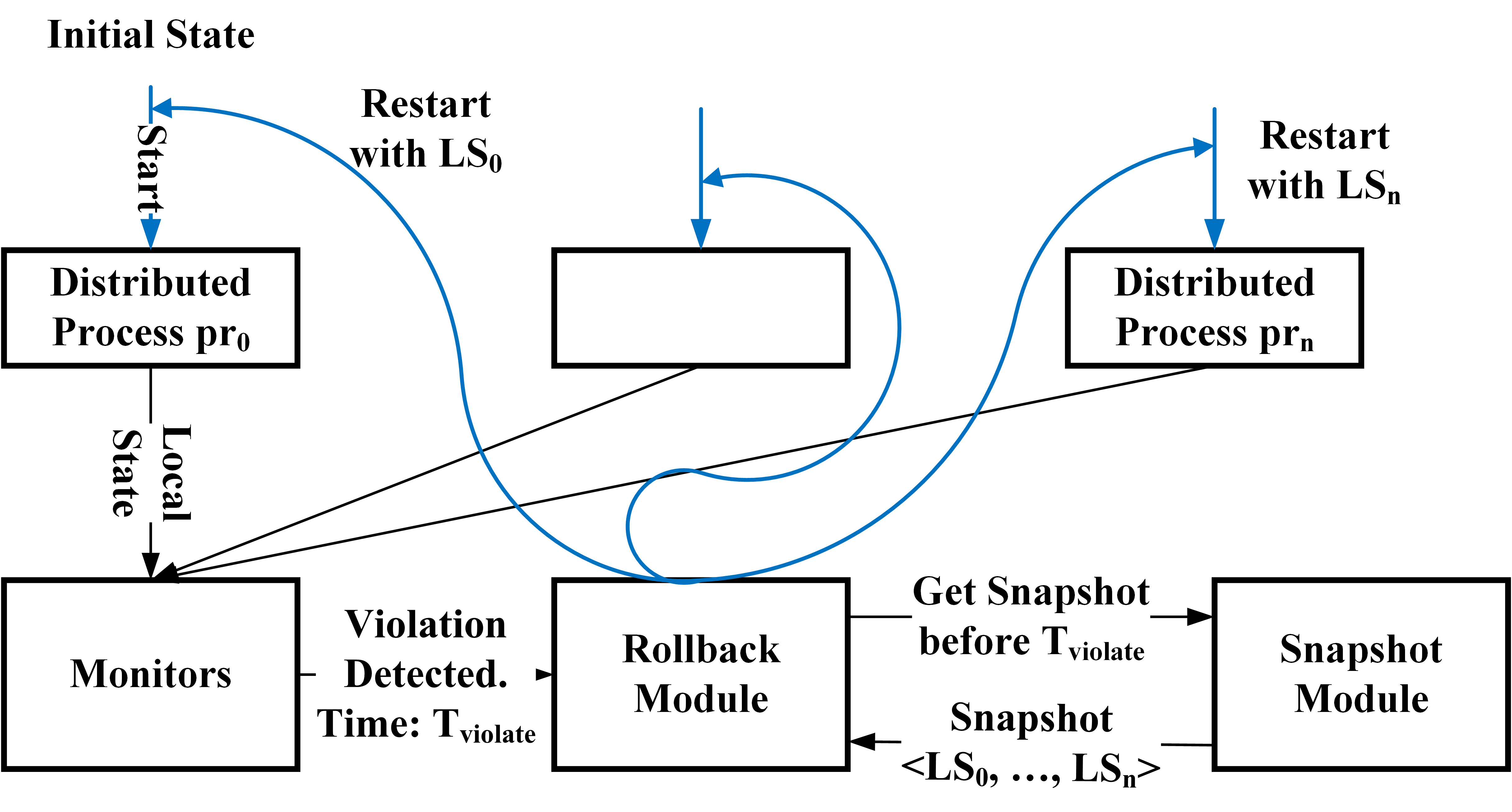
Figure 2: An overall framework for optimistic execution in key-value store

The approach in Retroscope can be further optimized by identifying the cause of the rollback. For instance, recall the example from the Introduction that considers a graph application and requires that two clients do not operate on neighboring nodes simultaneously. Suppose a violation is detected due to clients $C_{1}$ and $C_{2}$ operating on neighboring nodes $V_{1}$ and $V_{2}$. In this case, we need to rollback $C_{1}$ and $C_{2}$ to states before they operated on $V_{1}$ and $V_{2}$. However, clients that do not depend upon the inconsistent values of nodes $V_{1}$ and $V_{2}$ need not be rolled back. Hence, unnecessary rollback can be avoided.

5 Monitoring Module

The monitoring module is responsible for monitoring and detecting violation of the global predicate of interest in a distributed system. The structure of the module is as shown in Figure 3. It consists of local predicate detectors attached to each server and the monitors independent of the servers. The local predicate detector caches the state of its host server and sends information to the monitors. This is achieved by intercepting the PUT requests for variables that may affect the predicate being monitored. The monitors run predicate detection algorithm based on the information received to determine if the global predicate of interest $P$ has been violated.

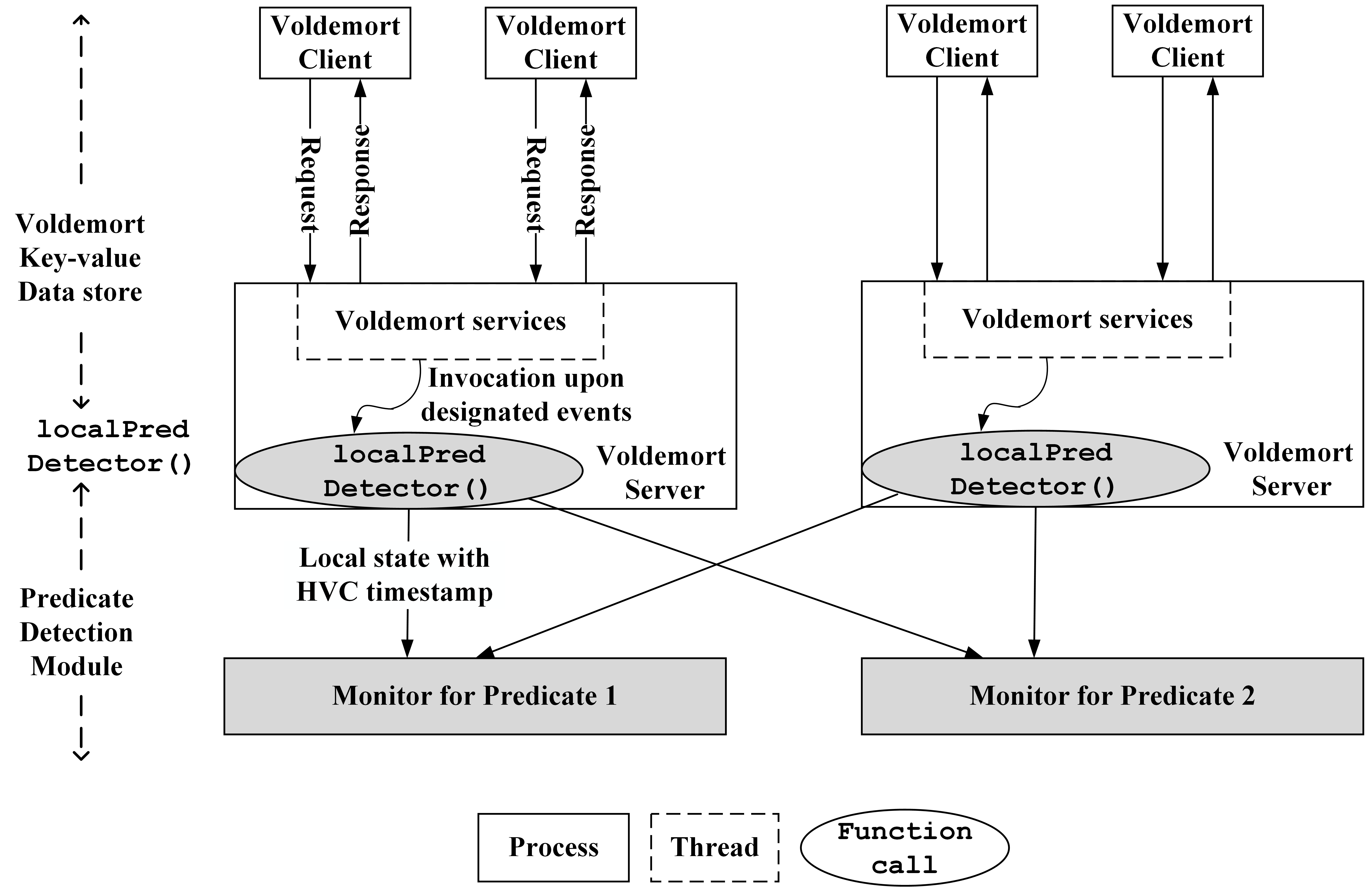
Figure 3: Architecture of predicate detection module

We anticipate that the predicate of interest $P$ is a conjunction of all constraints that should be satisfied during the execution. In other words, $P$ is of the form $P_{1}\wedge P_{2}\wedge\cdots P_{l}$ where each $P_{i}$ is a constraint (involving one or more processes) that the program is expected to satisfy. Each $P_{i}$ can be of different types (such as linear or semilinear). The job of the monitoring module is to identify an instance where $P$ is violated, i.e., to determine if there is a consistent cut where $\neg P_{1}\vee\neg P_{2}\vee\cdots\neg P_{l}$ is true. In order to monitor multiple predicates, the designer can have multiple monitors with one monitor for each predicate $P_{i}$ or one monitor for all predicates $P_{i}$’s. In the former case, the detection latency is small but the overheads can be unaffordable when the number of predicates is large since we need many monitor processes. In the latter case, the overhead is small but the detection latency is long. We adopt a compromise: our monitoring module consists of multiple monitors and each monitor is responsible for multiple predicates. The predicates are assigned to the monitors based on the hash of the predicate names in order to balance the monitors’ workload.

The number of monitors equals the number of servers and the monitors are distributed among the machines running the servers. We have done so to ensure that the cost of the monitors is accounted for in experimental results while avoiding overloading a single machine. An alternative approach is to have monitors on a different machine. In this case, the trade-off is between CPU cycles used by the monitors (when monitors are co-located with servers) and communication cost (when monitors are on a different machine). Our experiments suggest that in the latter approach (monitors on a different machine) monitoring is more efficient. However, since there is no effective way to compute the increased cost (of machines in terms of money), we report results where monitors are on the same machines as the servers.

Each (smaller) predicate $P_{i}$ is a boolean formula on the states of some variables. Since any boolean formula can be converted to a disjunctive normal form, users can provide the predicates being detected ($\neg P_{i}$’s) in disjunctive normal form. We use the XML format to represent the predicate. For example, the semilinear predicate, says $\neg P_{1}\equiv(x_{1}=1\land y_{1}=1)\lor z_{2}=1$, in XML format is shown in Figure 4. Observe that this XML format also identifies the type of the predicate (linear, semi-linear, etc.) so that the monitor can decide the algorithm to be used for detection.

<predicate>
  <type>semilinear</type>
  <conjClause>
    <id>0</id>
    <var>
      <name>x2</name> <value>1</value>
    </var>
    <var>
      <name>y2</name> <value>1</value>
    </var>
  </conjClause>
  <conjClause>
    <id>1</id>
    <var>
      <name>z2</name> <value>1</value>
    </var>
  </conjClause>
</predicate>

Figure 4: XML specification for $\neg P\equiv(x_{1}=1\land y_{1}=1)\lor z_{2}=1$

Implementation of local predicate detectors. Upon the execution of a PUT request, the server calls the interface function localPredicateDetector which examines the state change and sends a message (also known as a candidate) to one or more monitors if appropriate. Note that not all state changes cause the localPredicateDetector to send candidates to the monitors. The most common example of this is when the changed variable is not relevant to the predicates being detected. Other examples depend upon the type of predicate being detected. As an illustration, if predicate $\neg P$ is of the form $x_{1}\wedge x_{2}$ then we only need to worry about the case where $x_{i}$ changes from $false$ to $true$.

A candidate sent to the monitor of predicate $P_{i}$ consists of an HVC interval and a partial copy of the server local state containing variables relevant to $P_{i}$. The HVC interval is the time interval on the server when $P_{i}$ is violated, and the local state has the values of variables which make $\neg P_{i}$ true.

For example, assume the global predicate of interest to be detected is $\neg P\equiv\neg P_{1}\vee\neg P_{2}\cdots\vee\neg P_{m}$ where each $\neg P_{j}$ is a smaller global predicate. Assume that monitor $M_{j}$ is responsible for detection of predicate $\neg P_{j}$. Consider a smaller predicate, says $\neg P_{2}$, and for the sake of the example, assume that it is a conjunctive predicate, i.e. $\neg P_{2}\equiv(\neg LP_{2}^{1})\wedge(\neg LP_{2}^{2})\wedge...(\neg LP_{2}^{n})$ where $n$ is the number of servers. We want to detect when $\neg P_{2}$ becomes true. On a server, say server $i$, the local predicate detector will monitor the corresponding local predicate $\neg LP_{2}^{i}$ (or $\neg LP_{2}$ for short, in the context of server $i$ as shown in Figure 5). Since $\neg P_{2}$ is true only when all constituent local predicates are true, server $i$ only has to send candidates for the time interval when $\neg LP_{2}$ is true. In Figure 5, upon the first PUT request, no candidate is sent to monitor $M_{2}$ because $\neg LP_{2}$ is false during interval $[HVC_{i}^{0},HVC_{i}^{1}]$. After serving the first PUT request, the new local state makes $\neg LP_{2}$ true, starting from the time $HVC_{i}^{2}$. Therefore upon the second PUT request, a candidate is sent to monitor $M_{2}$ because $\neg LP_{2}$ is true during the interval $[HVC_{i}^{2},HVC_{i}^{3}]$. This candidate transmission is independent of whether $\neg LP_{2}$ is true or not after the second PUT request is served. It depends on whether $\neg LP_{2}$ is true after execution of the previous PUT request. That is why, upon the second PUT request, a candidate is also sent to monitor $M_{3}$ but none is sent to $M_{1}$. However, if the predicate is not a linear predicate, then upon a PUT request for a relevant variable, the local predicate detector has to send a candidate to the associated monitor anyway.

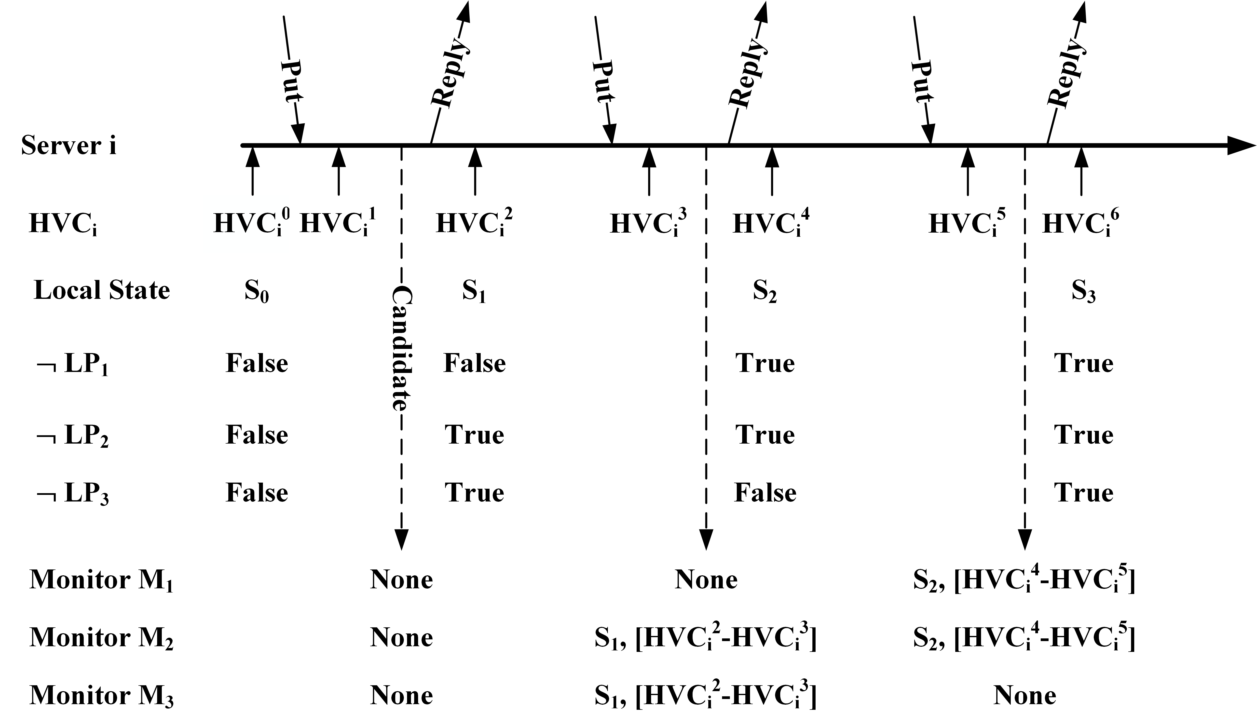
Figure 5: Illustration of candidates sent from a server to monitors corresponding to three conjunctive predicates. If the predicate is semilinear, the candidate is always sent upon a PUT request of relevant variables.

Implementation of the monitors. The task of a monitor is to determine if some smaller predicate $P_{i}$ under its responsibility is violated, i.e., to detect if a consistent state on which $\neg P_{i}$ is true exists in the system execution. The monitor constructs a global view of the variables relevant to $P_{i}$ from the candidates it receives. The global view is valid if all candidates in the global view are pairwise concurrent.

The concurrence/causality relationship between a pair of candidates is determined as follows: suppose we have two candidates $Cand_{1},Cand_{2}$ from two servers $S_{1},S_{2}$ and their corresponding HVC intervals $[HVC_{1}^{start},HVC_{1}^{end}],[HVC_{2}^{start},HVC_{2}^{end}]$. Without loss of generality, assume that $\neg(HVC_{1}^{start}>HVC_{2}^{start})$ (cf. Figure 6).

• If $HVC_{2}^{start}<HVC_{1}^{end}$ then the two intervals have common time segment and $Cand_{1}\|Cand_{2}$.

• If $HVC_{1}^{end}<HVC_{2}^{start}$, and $HVC_{1}^{end}[S_{1}]\leq HVC_{2}^{start}[S_{2}]-\epsilon$ then interval one is considered happens before interval two. Note that $HVC[i]$ is the element corresponding to process $i$ in HVC. In this case $Cand_{1}\rightarrow Cand_{2}$

• If $HVC_{1}^{end}<HVC_{2}^{start}$, and $HVC_{1}^{end}[S_{1}]>HVC_{2}^{start}[S_{2}]-\epsilon$, this is the uncertain case where the intervals may or may not have common segment. In order to avoid missing possible violations, the candidates are considered concurrent.

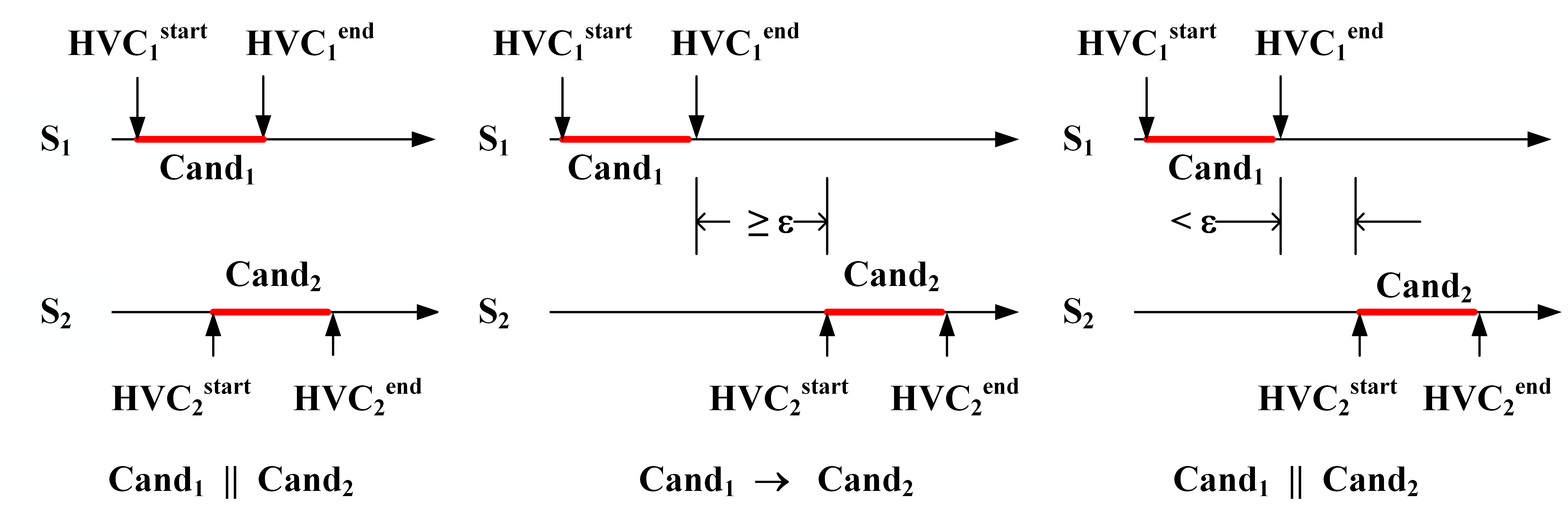
Figure 6: Illustration of causality relation under HVC interval perspective

When a global predicate is detected, the monitor informs the administrator or triggers a designated process of recovery. We develop detection algorithms for the monitors of linear predicates and semilinear predicates based on [13, 14] as shown in Algorithm 1 and Algorithm 2. Basically, the algorithms have to identify the correct candidates to update the global state ($GS$) so that we would not have to consider all possible combinations of $GS$ as well as not miss the possible violations. In linear (or semilinear) predicates, these candidates are forbidden (or semi-forbidden) states. Forbidden states are states such that if we do not replace them, we would not be able to find the violation. Therefore, we must advance the global state along forbidden states. Semi-forbidden states are states such that if we advance the global state along them, we would find a violation if there exists any. The procedure of advancing the global snapshot $GS$ along a local state $s$ ($s$ belongs to $GS$) means the successor of $s$ is added to $GS$. The successor of a local state $s$ is the next local state after $s$ on the same process. As $s$ is replaced by its successor, the global snapshot $GS$ “advances” forward. When advancing global state along a candidate (which contains a local state), that candidate may not be concurrent with other candidates existing in the global state. In that case, we have to advance the candidates to make them consistent. This is done by consistent(GS) in the algorithm. If we can advance global state along a candidate without calling consistent(GS), that candidate is called an eligible state. The set of all eligible states in the global state is denoted as eligible(GS) in the algorithms. For a more detailed discussion of linear and semi-linear predicates, we refer to [14].

Algorithm 1 Linear predicate monitor algorithm [13]

1:Input:

2:     $P$ $\triangleright$ global linear predicate to monitor

3:Variable:

4:     $GS$ $\triangleright$ global state

5:Initialization:

6:     $GS\leftarrow$ set of initial local states

7:while P(GS)==true do

8:     Find forbidden local state $s\in GS$

9:     $GS\leftarrow GS\cup{succ(s)}$ $\triangleright$ advance $GS$ along $s$

10:     consistent($GS$) $\triangleright$ make $GS$ consistent

11:end while

12:return $GS$

Algorithm 2 Semilinear predicate monitor algorithm [14]

1:Input:

2:     $P$ $\triangleright$ global semilinear predicate to monitor

3:Variable:

4:     $GS$ $\triangleright$ global state

5:Initialization:

6:     $GS\leftarrow$ set of initial local states

7:while P(GS)==true do

8:     Find a local state $s\in GS$ such that $s\in eligible(GS)$ and $s$ a semi-forbidden state of $P$ in $GS$.

9:     $GS\leftarrow GS\cup{succ(s)}$ $\triangleright$ advance $GS$ along $s$

10:end while

11:return $GS$

After a consistent global state $GS$ is obtained, we evaluate whether predicate $P$ is violated at this global state ($P(GS)=true$ means $P$ is satisfied, $P(GS)=false$ means $P$ is violated). If $P$ is violated, the algorithms return the global snapshot $GS$ as the evidence of the violation. Note that the monitors will keep running even after a violation is reported so that possible violations in the future will not be missed. This is the case when the applications, after being informed about the violation and rolling back to a consistent checkpoint before the moment when the violation occurred, continue their execution and violations occur again. Hence the monitors have to keep running in order to detect any violations of $P$.

The way we evaluate $P$ on global state $GS$ is slightly different from the algorithms in [14, 13, 12, 22]. In those algorithms, the candidates are sent directly from the clients containing the states of the clients. In our algorithms, the candidates are sent from the servers containing the information the servers know about the states of the clients that have been committed to the store by the clients. Note that, in a key-value store, the clients use the server store for sharing variables and committing updates. Therefore, the states of clients will eventually be reflected at the server store. Since the predicate $P$ is defined over the states of the clients, in order to detect violations of $P$ from the states stored at the server, we have to adapt the algorithms in [14, 13, 12, 22] to consider that difference. Furthermore, the state of a client can be stored slightly differently at different servers. For example, a PUT request may be successful at the regional server but not successful at remote servers. In that case, assuming we are using eventual consistency, the regional server store will have the update while remote stores do not have the update. Our algorithms also consider this factor when evaluating $P$. For example, suppose variable $x$ has version $v_{1}$ at a server and version $v_{2}$ at another server. Suppose that if $x=v_{1}$ then $P$ is violated, and if $x=v_{2}$ then $P$ is satisfied. To avoid missing possible violations, our algorithms check all available versions of $x$ when evaluating $P$.

Since our algorithms are adapted from [14, 13, 12, 22], the correctness of our algorithms follow from those existing algorithms. We refer to [14, 13, 12, 22] for more detailed discussion and proof of correctness of the algorithms.

Handling a large number of predicates. When the number of predicates to be monitored is large (e.g. hundreds of thousands, as in Social Media Analysis application in next section or in graph-based applications discussed in the Introduction), it is costly to maintain monitoring resources (memory, CPU cycles) for all of them simultaneously. That not only slows down the detection latency but also consumes all the resources on the machines hosting the monitors (for example, we received OutOfMemoryError error when monitoring tens of thousands of predicates simultaneously). However, we observe that not all predicates are active at the same time. Only predicates relevant to the nodes that the clients are currently working on are active. A predicate is considered inactive when there is no activity related to that predicate for a predetermined period of time, and therefore the evaluation of that predicate is unchanged. Consequently, the monitors can clean up resources allocated for that predicate to save memory and processing time.

Automatic inference of predicate from variable names. This feature is also motivated by applications where the number of predicates to be monitored is large such as the graph-based applications. In this case, it is impossible for the users to manually specify all the predicates. However, if the variables relevant to the predicates follow some naming convention, our monitoring module can automatically generate predicates on-demand. For example, in graph-based applications, the predicates are the mutual exclusions on any edge whose endpoints are assigned to two different clients. Let $A$ and $B$ are two such nodes and $A\_B$ is the edge between them. Assume $A<B$. If the clients are using Peterson’s mutual exclusion, the predicate for edge $A\_B$ will be

$$\neg P_{A\_B}\equiv(flagA\_B\_A=true\wedge turnA\_B="A")$$

$$\wedge(flagA\_B\_B=true\wedge turnA\_B="B")$$

When a server receives a PUT request from some client for a variable whose name is either flagA_B_A, or flagA_B_B, or turnA_B, it knows that the client is interested in the lock for edge $A\_B$ and the local predicate detector will generate the predicate for edge $A\_B$ so that the monitors can detect if the mutual exclusion access on edge $A\_B$ is violated. On the other hand, if the servers never see requests for variables flagA_B_A, flagA_B_B, and turnA_B, then both nodes $A$ and $B$ are assigned to the same client and we do not need the mutual exclusion predicate for edge $A\_B$.

6 Rollback from Violations

6.1 Rollback Mechanism

While inconsistency is possible with eventual consistency, it is rare [1] given that networks are reliable and data conflicts are infrequent. However, such inconsistencies and data conflicts can arise and, hence, one needs to deal with these conflicts if we are using an application that relies on sequential consistency. We discuss the rollback approaches for such scenarios.

One possible approach for rollback, especially if violations can be detected quickly is as follows: We partition the work assigned to each client in terms of several tasks. Each task consists of two phases (cf. Figure 7): (1) Read phase: the client obtains all necessary locks for all nodes in the task, reading the necessary data, and identify the values that need to be changed. However, all updates in this phase are done in local memory. (2) Write phase: the client writes the data that they are expected to change and reflect it in the data store.

In such a system, a violation could occur if clients C1 and C2 are accessing the same data simultaneously. For sake of discussion, suppose that client C1 started accessing the data before C2. Now, if the detection of violation is quick then detection would occur before client C2 enters the write phase. In this case, client C2 has not performed any changes to the key-value store. In other words, client C2 can re-start its task (that involves reading the data from the key-value store) to recover from the violation.

With this intuition, we can provide recovery as follows: When a violation is detected, if the client causing the violation is in the read phase, it aborts that task and starts that task again. On the other hand, if a client is in write phase (and this can happen to at most one task if detection is quick enough) then it continues its task normally. Note that with this approach, it is possible that two clients that result in a violation are both in the read phase. While one of the clients could be allowed to continue normally, this requires clients to know the status of other clients. We do not consider this option as it is expected that in most applications clients do not communicate directly. Rather, they communicate only via the key-value store. We utilize this approach in our rollback mechanism. In particular, when detection is quick, we use the Algorithm 3 for rollback (cf. Figure 7 and Algorithm 3).

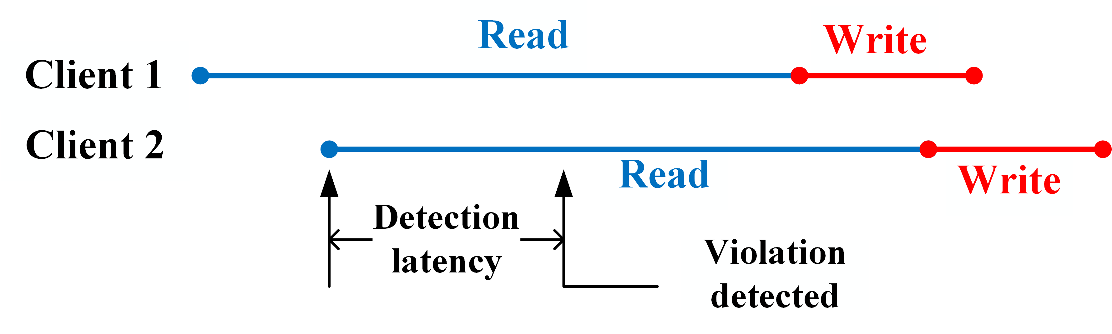
Figure 7: Two client tasks involved in a violation. Since detection latency is much smaller than the Read phase time, violation will be notified within Read phase of the current task of at least one client.

Other approaches for rollback are as follows:

• Rollback via Retroscope[11]. The most general approach is to utilize an algorithm such as RetroScope [11]. Specifically, it allows one to rollback the state of the key-value store to an earlier state. The time, $t$, of rollback is chosen in such a way that there are no violations before time $t$. Upon such a rollback, we can determine the phases the clients are in at time $t$. If a client is in the read phase at time $t$, it will abort its current task and begin it again. And, if the client is in a write phase, it will finish that phase. Note that since there are no conflicts until time $t$, such write phases will not result in conflicts.

  While this approach is most general, it is also potentially expensive. Hence, some alternate approaches are as follows:

• Use of Self-Stabilizing Algorithms. One possibility is if we are using a self-stabilizing algorithm. An algorithm is self-stabilizing if it is guaranteed to recover to a legitimate state even in the presence of arbitrary state perturbation. In [23], it is shown that if the underlying algorithm is self-stabilizing then we can simply ignore the violations as we can treat it as a state perturbation and the algorithm is already designed to handle it. In this case, there is neither a need for monitoring or rollback.

• Use of Application-Specific Rollbacks. Another possibility is application specific rollback. To illustrate this, consider an example of graph coloring. For sake of illustration, consider that we have three nodes A, B, C, arranged in a line with node B in the middle. Each node may have additional neighbors as well. Node A chooses its color based on the colors of its neighbors. Subsequently, node B chooses its color based on node A (and other neighbors of B). Afterward, C chooses its color based on B (and other neighbors of C). At this point, node B is required to rollback, it can still choose its color based on the new color of node C while still satisfying the constraints of graph coloring. In other words, in this application, we do not need to worry about cascading rollback.

Algorithm 3 Rollback algorithm at a client

1:for taskId = clientFirstTask to clientLastTask do

2:     while (performTask(taskId) == False) do

3:     end while

4:end for

5:

6:function performTask($taskId$)

7:     Obtain relevant locks

8:     Read information from data-store

9:     Compute new values

10:     if Violation is received then

11:         Release locks

12:         return False $\triangleright$ abort

13:     end if

14:     Write new values to data-store

15:     return True $\triangleright$ success

16:end function

6.2 Dealing with Potential of Livelocks

One potential issue with rollback is a possibility of livelocks. Specifically, if two clients C1 and C2 rollback and continue their execution then the same violation is likely to happen again. We consider the following choices for dealing with such livelocks.

• Random Backoff. Upon rollback, clients perform a random backoff. With backoff, the requests for locks from clients arrive at different times in the key-value store. Hence, the second client is likely to observe locks obtained by the first client in a consistent manner. In turn, this will reduce the possibility of the same violation to recur.

• Reordering of Tasks. If the work assigned to clients consists of several independent tasks, then clients can reorder the tasks upon detecting a violation. In this case, the clients involved in the rollback are likely to access different data and, hence, the possibility of another violation is reduced.

• Moving to Sequential Consistency. If the number of violations is beyond a certain threshold, clients may conclude that the cost of rollback is too high and, hence, they can move to sequential consistency. While this causes one to lose the benefits of an eventual consistent key-value store, there would be no need for rollback or monitoring.

7 Evaluation Results and Discussion

7.1 Experimental Setup

System configurations. We ran experiments on Amazon AWS EC2 instances. The servers ran on M5.xlarge instances with 4 vCPUs, 16 GB RAM, and a GP2 general-purpose solid-state drive storage volume. The clients ran on M5.large instances with 2 vCPUs and 8 GB RAM. The EC2 instances were located in three AWS regions: Ohio, U.S; Oregon, U.S; Frankfurt, Germany.

We also ran experiments on our local lab network which is set up so that we can control network latency. We used 9 commodity PCs, 3 for servers, 6 for clients, with configurations as in Table 1. Each client machine hosted multiple client processes, while each server machine hosted one Voldemort server process.

Table 1: Machine configuration in local lab experiments

Machine	CPU	RAM
Server machine 1, 2	4 Intel Core i5 3.33 GHz	4 GB
Server machine 3	4 Intel Core i3 3.70 GHz	8 GB
Client machine 1, 2	4 Intel Core i5 3.33 GHz	4 GB
Client machine 3, 4	Intel Core Duo 3.00 GHz	4 GB
Client machine 5	4 AMD Athlon II 2.8 GHz	6 GB
Client machine 6	4 Intel Core i5 2.30 GHz	4 GB

On the local network, we control the delay by placing proxies between the clients and the servers. For all clients on the same physical machine, there is one proxy process for those clients. All communication between those clients and any server is relayed through that proxy (cf. Figure 8). Due to the proxy delays, machines are virtually arranged into three regions as in Figure 9. Latency within a region is small ($2\text{\,}\mathrm{ms}$) while those across regions are high and tunable (e.g. $50\text{\,}\mathrm{ms}100\text{\,}\mathrm{ms}$). Since Voldemort uses active replication, we do not place proxies between servers. The latency in the proxies is simulated to follow the Gamma distribution [24, 25].

We considered replication factors ($N$) of 3 and 5. The parameters $R$ (required reads) and $W$ (required writes) are chosen to achieve different consistency models as shown in Table 2. The number of servers is equal to the replication factor $N$. The number of clients is varied between 15 and 90.

Table 2: Setup of consistency models with $N$ (replication factor), $R$ (required reads), and $W$ (required writes)

N	R	W	Abbreviation	Consistency model
3	1	3	N3R1W3	Sequential
	2	2	N2R2W2	Sequential
	1	1	N3R1W1	Eventual
5	1	5	N5R1W5	Sequential
	3	3	N5R3W3	Sequential
	1	1	N5R1W1	Eventual

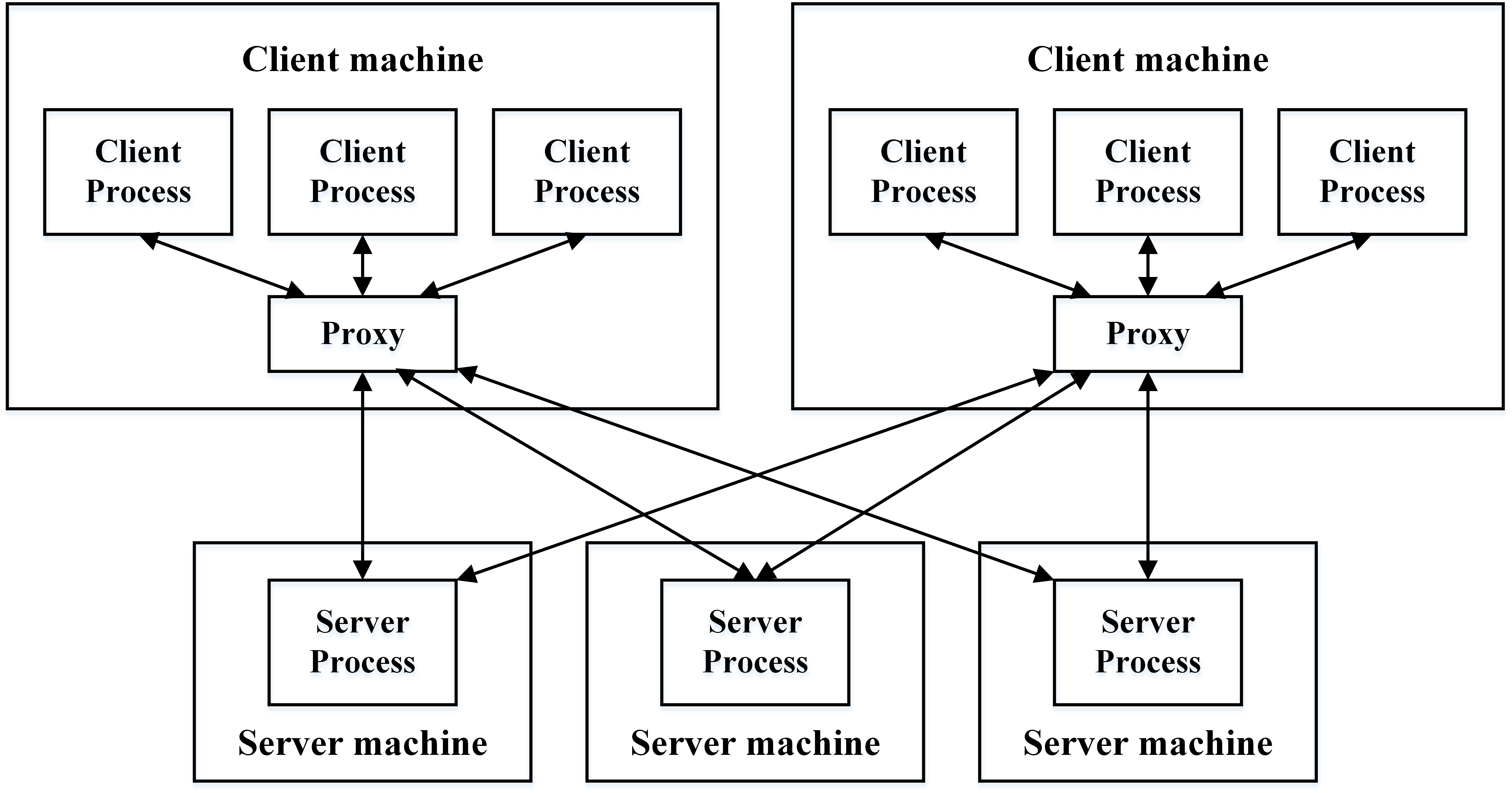
Figure 8: Simulating network delay using proxies

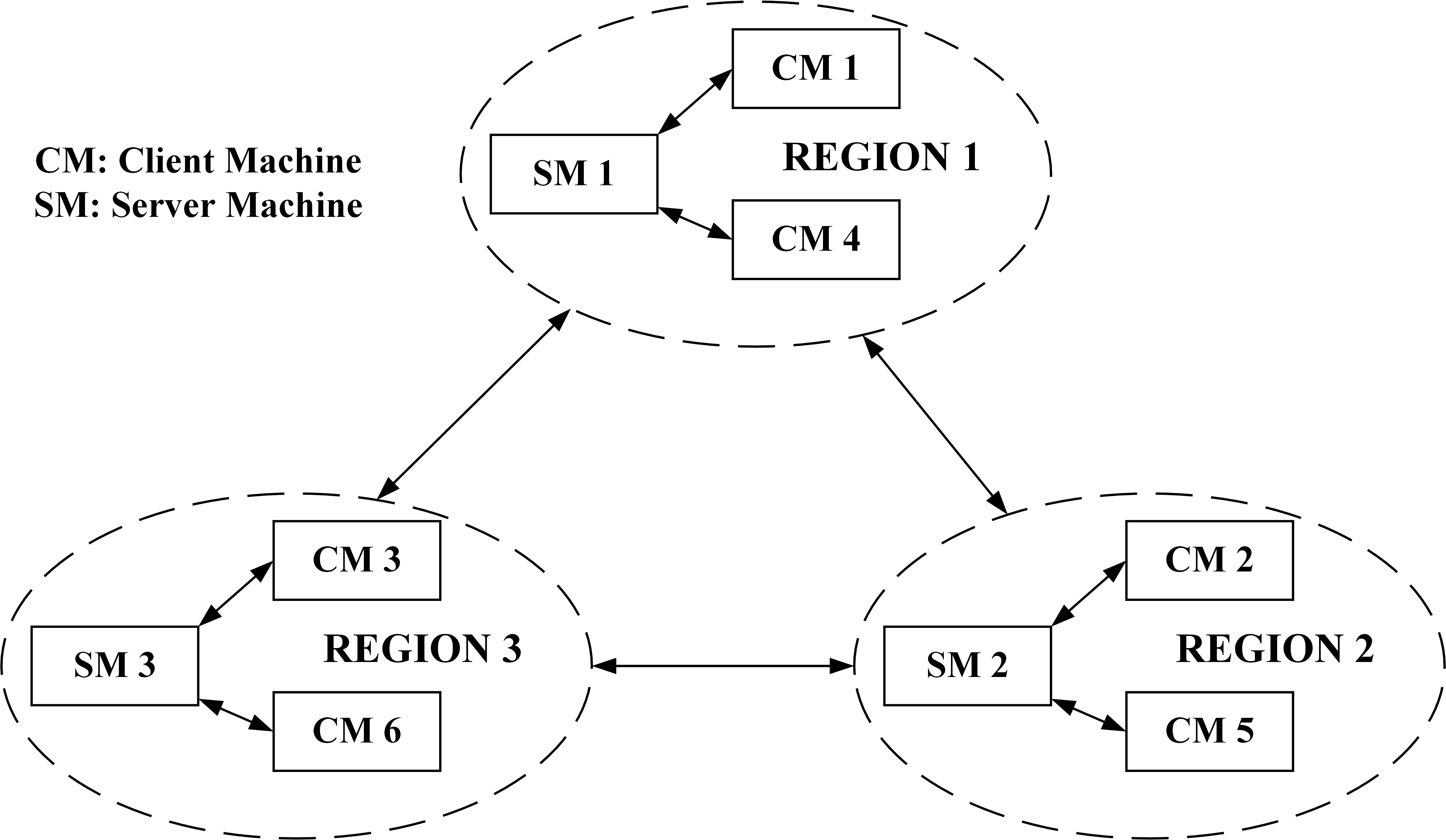
Figure 9: Network arrangement with proxies

Test cases. In our experiments, we used 3 case studies: Social Media Analysis, Weather Monitoring, and Conjunctive.

The application motivated by Social Media Analysis considers a large graph representing users and their connections. The goal of clients is to update the state of each user (node) based on its connections. For the sake of illustration in our analysis, the attribute associated with each user is a color and the task is to assign each node a color that is different from its neighbors. We use the tool networkx [26] to generate input graphs. There are two types of graph: (1) Power-law clustering graph that simulates the power-law degree and clustering characteristics of social networks, and (2) Random 6-regular graph in which each node has 6 adjacent edges and the edges are selected randomly. The reason we use random regular graphs is that they are the test cases where the workload is distributed evenly between clients and throughout the execution. The graphs have $50,000$ nodes with about $150,000$ edges. Each client is assigned a set of nodes to be colored and run a distributed coloring algorithm [27].

Since the color of a node is chosen based on its neighbors’ colors, while a client $C_{1}$ is coloring node $v_{1}$, no other client is updating the colors of $v_{1}$’s neighbors. The goal of the monitors is to detect violation of this requirement. This requirement can be viewed as a mutual exclusion (semi-linear) predicate where a client going to update the color of $v_{1}$ has to obtain all the exclusive locks associated with the edges incident to $v_{1}$. Mutual exclusion is guaranteed if clients use Peterson’s algorithm and the system provides sequential consistency [10]. However, it may be violated in the eventual consistency model. To avoid deadlock, clients obtain locks in a consistent order. For example, let $A\_B$ and $C\_D$ are the locks associated with the edges between nodes $A$ and $B$, and $C$ and $D$ respectively. Assume $A<B$ and $C<D$. Then lock $A\_B$ is obtained before $C\_D$ when $A<C$ or when $A=C$ and $B<D$.

The number of predicates being monitored in this test case is proportional to the number of edges.

We note that the task performed by each client (i.e., choosing the color of a node) is just used as an example. It is easily generalized for other analysis of Social Media Graph (e.g., finding clusters, collaborative learning, etc.)

The application motivated by Weather Monitoring task considers a planar graph (e.g. a line or a grid) where the state of each node is affected by the state of its neighbors. In a line-based graph, all the nodes of the graph are arranged on a line and each client is assigned a segment of the line. In a grid-based graph, the graph nodes are arranged on a grid. The clients are also organized as a grid and each client is responsible for a section of the grid of nodes. In this application, we model a client that updates the state of each node by reading the state of its neighbors and updating its own state. This application can be tailored to vary the ratio of GET/PUT request. This application is relevant to several practical planar graph problem such as weather forecasting [28], radio-coloring in wireless and sensor network [29], computing Voronoi diagram [30].

Finally, the Conjunctive application is an instance of distributed debugging where the predicate being detected (i.e., $\neg P$) is of the form $P_{1}\wedge P_{2}\wedge\cdots\wedge P_{l}$. Each local predicate $P_{i}$ becomes true with a probability $\beta$ and the goal of the monitors is to determine if the global conjunctive predicate $\neg P$ becomes true. In this application, we monitor multiple conjunctive predicates simultaneously. Since we can control how frequently these predicates become true by varying $\beta$, we can use it mainly to assess monitoring latency and stress the monitors. Conjunctive predicates are also useful in distributed testing such as to specify breakpoints.

Performance metrics and measurement. We use throughput as the performance metrics in our experiments. Throughput can be measured at two perspectives: application, and Voldemort server. The two perspectives are not the same but related. One application request triggers multiple requests at Voldemort client. For example, one application PUT request is translated into one GET_VERSION request (to obtain the last version of the key) and one PUT request (with a new incremented version) at the Voldemort client library. Then each Voldemort client request causes multiple requests at servers due to replication. Failures and timeout also make the counts at the applications and the servers differ. For example, an application request is served and counted at a server but if the server response is lost or arrives after the timeout, the request is considered unsuccessful and thus not counted at the application. Generally, servers’ counts are greater than applications’ counts. In our experiments, we use the aggregated measurement at servers to assess the overhead of our approach since the monitors directly interfere with the operation of the server, and use aggregated measurement at applications to assess the benefit of our approach because that measurement is close to users’ perspective. Hence, in the following sections, for the same experiment, we note that the measurements used for overhead and benefit evaluation are different.

Results stabilization. We ran each experiment three times and used the average as the representative results for that experiment. Figure 10 shows the stabilization of different runs of an experiment. Note that the values are aggregated from all applications. We observe that in every run, after a short period of initialization, the measurements converge on a stable value. When evaluating our approach, we use the values measured at the stable phase. We also note that the aggregated throughput in Figure 10 is not very high but expected. The pairwise round-trip latency between three AWS regions (Ohio, Oregon, Frankfurt) were $76\text{\,}\mathrm{ms}103\text{\,}\mathrm{ms}163\text{\,}\mathrm{ms}$. The average round-trip latency was $114\text{\,}\mathrm{ms}$. On M5.xlarge EC2 instances with a GP2 storage volume, the average I/O latency for a read and a write operation was roughly $0.3\text{\,}\mathrm{ms}$ and $0.5\text{\,}\mathrm{ms}$, respectively. We will roughly estimate the cost of a GET request since in Social Media Analysis, most operations are GET requests to read lock availability and colors of neighbors. Assume eventual consistency R1W1 is used, a GET request is executed by Voldemort client in two steps:

• Perform parallel request: client simultaneously sends GET requests to all servers (N = 3) and wait for responses with a timeout of $500\text{\,}\mathrm{ms}$. The wait is over when either client gets responses from all servers or the timeout expires. In this case, the client will get all responses in about $114.3\text{\,}\mathrm{ms}$ ($114\text{\,}\mathrm{ms}$ for communication delay, and $0.3\text{\,}\mathrm{ms}$ for the read operation processing time at the server).

• Perform serial request: client checks if it has received enough required responses. If not, it has to send addition GET requests to servers to get enough number of responses. If after the additional requests, the required number of responses is not met, the GET request is considered unsuccessful. Otherwise, the result is returned. In the current case, the number of responses received (3) is greater than the required (R = 1). Thus this step is skipped.

From this discussion, a GET request takes roughly $115\text{\,}\mathrm{ms}$ to complete, on average. Since GET is the dominating operation in the Social Media Analysis application, with 15 clients, the expected aggregated throughput is $\frac{15}{0.1143}\approx$ $131\text{\,}\mathrm{o}\mathrm{p}\mathrm{s}$. The average throughput measured in experiments was $132\text{\,}\mathrm{o}\mathrm{p}\mathrm{s}$ (cf. Figure 10).

If we run experiments where all machines are in the same region but in different availability zones, the aggregated throughput will be higher (cf. Figure 12). For example, in the AWS North Virginia region, the average round-trip latency within an availability zone was about $0.5\text{\,}\mathrm{ms}$, and between different availability zones was about $1.4\text{\,}\mathrm{ms}$. Based on the discussion about GET request above, a GET request takes roughly $0.8\text{\,}\mathrm{ms}$ ($0.5\text{\,}\mathrm{ms}$ for network latency within an availability zone plus $0.3\text{\,}\mathrm{ms}$ for processing read request at the server). Similarly, a GET_VERSION request takes $0.8\text{\,}\mathrm{ms}$. Since we are using R1W1 configuration, an actual PUT request can be satisfied by the server within the same availability zone. Thus, an actual PUT request takes roughly $1\text{\,}\mathrm{ms}$ ($0.5\text{\,}\mathrm{ms}$ for network latency within an availability zone plus $0.5\text{\,}\mathrm{ms}$ for write operation processing time at the server). A PUT request (consisting of a GET_VERSION request and an actual PUT request) takes roughly $1.8\text{\,}\mathrm{ms}$. Assume the workload consists of $50\text{\,}\mathrm{\char 37\relax}$ GETs and $50\text{\,}\mathrm{\char 37\relax}$ PUTs, then on average, a request takes $0.5\times 0.8+0.5\times 1.8=$ $1.3\text{\,}\mathrm{ms}$ = $0.001{}3\text{\,}\mathrm{s}$. With 10 clients, the expected aggregate throughput is $\frac{10}{0.0013}=$ $7,692\text{\,}\mathrm{o}\mathrm{p}\mathrm{s}$. If the workload consists of $75\text{\,}\mathrm{\char 37\relax}$ GETs and $25\text{\,}\mathrm{\char 37\relax}$ PUTs, a request takes $0.75\times 0.8+0.25\times 1.8=$ $1.05\text{\,}\mathrm{ms}$ = $0.001{}05\text{\,}\mathrm{s}$, and the expected aggregate throughput is $\frac{10}{0.00105}=$ $9,524\text{\,}\mathrm{o}\mathrm{p}\mathrm{s}$. In our experiments, the aggregate throughput measured for $50\text{\,}\mathrm{\char 37\relax}$ PUT and $25\text{\,}\mathrm{\char 37\relax}$ PUT was $7,782\text{\,}\mathrm{o}\mathrm{p}\mathrm{s}$ and $9,593\text{\,}\mathrm{o}\mathrm{p}\mathrm{s}$, respectively (cf. Figure 12(a) and 12(b)).

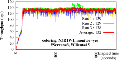
Figure 10: Illustration of result stabilization. The Social Media Analysis application is run three times on Amazon AWS with monitoring enabled. Number of servers ($N$) = $3$. Number of clients per server ($C/N$) = $5$. Aggregated throughput measured by Social Media Analysis application in three different runs and their average is shown. This average is used to represent the stable value of the application throughput.

7.2 Analysis of Throughput

Comparison of Eventual Consistency with Monitors vs. Sequential Consistency. As discussed in the introduction, one of the problems faced by the designers is that they have access to an algorithm that is correct under sequential consistency but the underlying key-value store provides a weaker consistency. In this case, one of the choices is to pretend as if sequential consistency is available but monitor the critical predicate $P$. If this predicate is violated, we need to rollback to an earlier state and resume the computation from there. Clearly, this approach would be feasible if the monitored computation with eventual consistency provides sufficient benefit compared with sequential consistency. In this section, we evaluate this benefit.

Figure 11(a) compares the performance of our algorithms for eventual consistency with monitors and sequential consistency without monitors in the Social Media Analysis application on the AWS environment. Using our approach, the client throughput was increased by $57\text{\,}\mathrm{\char 37\relax}$ (for N3R1W3) and $78\text{\,}\mathrm{\char 37\relax}$ (for N3R2W2). Note that the cost of a GET request is more expensive in N3R2W2 (the required number of positive acknowledgment is 2) than in N3R1W3 (the required acknowledgment is 1). Since in the Social Media Analysis application GET requests dominates, the application performs better in N3R1W3 than in N3R2W2.

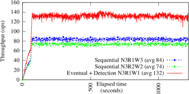
(a) Benefit=57% and 78%

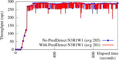
(b) Overhead on R1W1=1.4%

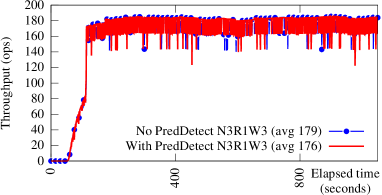
(c) Overhead on R1W3=1.7%

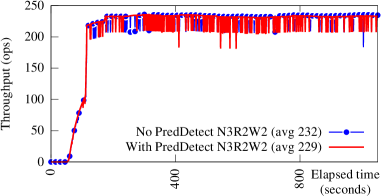
(d) Overhead on R2W2=1.3%

Figure 11: (AWS) Social Media Analysis application, 3 servers, 15 clients. The benefit of eventual consistency with monitors vs. sequential consistency without monitors (throughput improvement compared to R1W3 and R2W2 is 57% and 78%, respectively), and the overhead of running monitors on each consistency setting (the overhead is less than $2\%$).

Overhead of monitoring. A weaker consistency model allows the application to increase the performance on a key-value store as illustrated above. To ensure correctness, a weaker consistency model needs monitors to detect violations and trigger rollback recovery when such violations happen. As a separate tool, the monitors are useful in debugging to ensure that the program satisfies the desired property throughout the execution. In all cases, it is desirable that the overhead of the monitors is small so that they would not curtail the benefit of weaker consistency or make the debugging cost expensive.

Figures 11(b) 11(c), and 11(d) show the overhead of the monitors on different consistency settings in the Social Media Analysis application. The overhead was between $1\text{\,}\mathrm{\char 37\relax}2\text{\,}\mathrm{\char 37\relax}$. At its peak, the number of active predicates being monitored reached $20,000$ predicates. Thus, the overhead remains reasonable even with monitoring many predicates simultaneously.

7.3 Analysis of System and Application Factors

Impact of workload characteristics. In order to evaluate the impact of workload on our algorithms we ran the Weather Monitoring application where the proportional of PUT and GET was configurable. The number of servers was 5 and the number of clients was 10. The machines hosting the servers and clients were in the same AWS region (North Virginia, U.S.) but in 5 different availability zones. We choose machines in the same region to reduce the latency (to less than $2\text{\,}\mathrm{ms}$), thus increasing the throughput measure and stressing the servers and the monitors. If we put the clients and servers in different regions (e.g., Frankfurt Germany, Oregon USA, Ohio USA) then the throughput for 15 clients is low. To stress it further, we would have to add hundreds of clients which is very expensive. Hence, for the stress test, we put the servers and clients in the same region.

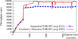
(a) PUT=25%. Benefit=18%

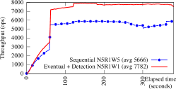
(b) PUT=50%. Benefit=37%

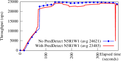
(c) PUT=50%. Overhead=4%

Figure 12: Benefit and overhead of monitors in Weather Monitoring application. Percentage of PUT requests is 25% and 50% Number of servers =$5$. Number of clients = $10$. Machines are on the AWS North Virginia region but in different availability zones.

From Figures 12(a) and 12(b), we find that when the percentage of PUT request increased from $25\text{\,}\mathrm{\char 37\relax}50\text{\,}\mathrm{\char 37\relax}$, the benefit over sequential consistency (N5R1W5 in this case) increased from $18\text{\,}\mathrm{\char 37\relax}37\text{\,}\mathrm{\char 37\relax}$. This is because the cost for a PUT request is expensive in N5R1W5 as a PUT request is successful only when it is confirmed by all 5 servers. Thus, when the proportion of PUT increases, the performance of N5R1W5 decreases. In such cases, sequential settings that balance R and W (e.g. N5R3W3) will perform better than sequential settings that emphasize W (e.g. N5R1W5). When GET requests dominate, it is vice versa (cf. Figure 11(a)). We also observe that, when PUT percentage increased and other parameters were unchanged, the aggregated throughput measured at clients decreased. That is because a PUT request consists of a GET_VERSION request (which is as expensive as a GET request) and an actual PUT request, therefore a PUT request takes a longer time to complete than a GET request does.

Regarding overhead, Figure 12(c) shows that the overhead was $4\text{\,}\mathrm{\char 37\relax}$ when PUT percentage was $50\text{\,}\mathrm{\char 37\relax}$. Note that in Weather Monitoring application, the number of predicates being monitored is proportional to the number of clients. Thus, the overhead remains reasonable even when monitoring several predicates simultaneously and the servers are stressed.

The number of violations detected in this experiment was only one instance in executions with a total time of $18,000\text{\,}\mathrm{ms}$. The violation was detected within $20\text{\,}\mathrm{ms}$.

Impact of network latency. We ran experiments on the local lab network (cf. Section 7.1) where the one-way latency within a region (cf. Figure 9) was $1\text{\,}\mathrm{ms}$ and one-way latency between regions varied from $50\text{\,}\mathrm{ms}100\text{\,}\mathrm{ms}$. The number of clients per each server varied between $10$ and $20$. The values in sub-columns “server” and “app” are the aggregate throughput measured at the servers and at the applications (unit is $\mathrm{o}\mathrm{p}\mathrm{s}$). In Table 3, the overhead is computed by comparing server measurements when the monitors are enabled and disabled. The benefit is computed by comparing application measurements on sequential consistency without monitoring to those on eventual consistency with monitoring. For example, when one-way latency is $50\text{\,}\mathrm{ms}$, if we run the Weather Monitoring application on N3R1W3 without monitoring, the aggregate server throughput is $649\text{\,}\mathrm{o}\mathrm{p}\mathrm{s}$ (Table 3, column 12 (N3R1W3 $\rightarrow$ server) and row 6 ($50\text{\,}\mathrm{ms}$ $\rightarrow$ Weather Monitoring $\rightarrow$ Monitor = no)) and the aggregate client throughput is $313\text{\,}\mathrm{o}\mathrm{p}\mathrm{s}$. If we run the same application on N3R1W3 with monitoring, the server throughput is $628\text{\,}\mathrm{o}\mathrm{p}\mathrm{s}$ (Table 3, column 12 and row 5). The overhead of monitoring Weather Monitoring application on N3R1W3 is $(649-628)/649=3.2\%$. The client throughput when run the same application on N3R1W1 with monitoring is $454\text{\,}\mathrm{o}\mathrm{p}\mathrm{s}$ (Table 3, column 7, row 5). Thus, the benefit of eventual consistency with monitoring vs. sequential consistency N3R1W3 is $(454-313)/313=45\%$.

From Table 3, as latency increases, the benefit of eventual consistency with monitoring vs. sequential consistency increases. For example when one-way latency increased from $50\text{\,}\mathrm{ms}100\text{\,}\mathrm{ms}$, in Social Media Analysis application, the benefit of eventual consistency with monitoring vs. sequential consistency R1W3 increased from $47\text{\,}\mathrm{\char 37\relax}60\text{\,}\mathrm{\char 37\relax}$. In the case of R2W2, the increase was from $65\text{\,}\mathrm{\char 37\relax}80\text{\,}\mathrm{\char 37\relax}$. This increase is expected because when latency increases, the chance for a request to be successful at a remote server decreases. Due to strict replication requirement of sequential consistency, the client will have to repeat the request again. On the other hand, on eventual consistency, requests are likely to be successfully served a local server and the client can continue regardless of results at remote servers. Hence, as servers are distributed in more geographically disperse locations, the benefit of eventual consistency is more noticeable. Regarding overhead, it was generally less than $4\text{\,}\mathrm{\char 37\relax}$. In all cases, the overhead was at most $8\text{\,}\mathrm{\char 37\relax}$.

Table 3: Overhead and benefit of monitors in local lab network. For Conjunctive and Weather Monitoring, PUT percentage is 50%.

Latency (ms)	Application	Client/ Server	Monitor	N3R1W1			N3R2W2				N3R1W3
				server	overhead	app	server	overhead	app	benefit	server	overhead	app	benefit
50	Conjunctive	20	yes	821	-0.2%	470	842	0.6%	375	25.3%	588	3.3%	337	40.7%
			no	819		470	847		375		608		334
	Weather Monitoring	20	yes	924	0.2%	454	795	7.1%	345	27.2%	628	3.2%	312	45.0%
			no	926		453	856		357		649		313
	Social Media Analysis	10	yes	560	0.2%	258	367	0.5%	156	65.4%	344	7.8%	174	47.4%
			no	561		267	369		156		373		175
100	Conjunctive	20	yes	476	0.4%	270	491	-0.2%	218	23.3%	354	0.0%	191	42.1%
			no	478		271	490		219		354		190
	Weather Monitoring	20	yes	544	0.7%	266	500	1.0%	209	28.5%	371	0.8%	176	49.4%
			no	548		273	505		207		374		178
	Social Media Analysis	10	yes	287	0.0%	135	236	0.0%	74	80%	185	-0.5%	86	60.7%
			no	287		133	236		75		184		84

7.4 Analysis of Violations and Detection Latency

Detection latency is the time elapsed between the violation of the predicate being monitored and the time when the monitors detect it. In our experiment with Social Media Analysis applications on eventual consistency (N3R1W1), in several executions of total $9,000\text{\,}\mathrm{s}$, we detected only 2 instances of mutual exclusion violations. Detection latency for those violations were $2,238\text{\,}\mathrm{ms}2,213\text{\,}\mathrm{ms}$. So for Social Media Analysis application, violations could happen on eventual consistency every $4,500\text{\,}\mathrm{s}$ on average.

In order to evaluate the detection latency of monitors with higher statistical reliability, we need experiments where violations are more frequent. In these experiments, the clients ran Conjunctive application in the same AWS configuration as Weather Monitoring application above. The monitors have to detect violations of conjunctive predicates of the form $P=P_{1}\wedge P_{2}\wedge\cdots P_{10}$. Furthermore, we can control how often these predicates become true by changing when local predicates are true. In these experiments, the rate of local predicate being true ($\beta$) was $1\text{\,}\mathrm{\char 37\relax}$, which was chosen based on the time breakdown of some MapReduce applications [31, 32]. The PUT percentage was $50\text{\,}\mathrm{\char 37\relax}$. The Conjunctive application is designed so that the number of predicate violations is large and to stress the monitors. We considered both eventual consistency and sequential consistency. Table 4 shows detection latency distribution of more than $20,000$ violations recorded in the Conjunctive experiments. Predicate violations are generally detected promptly. Specifically, $99.93\text{\,}\mathrm{\char 37\relax}$ of violations were detected in $50\text{\,}\mathrm{ms}$, $99.97\text{\,}\mathrm{\char 37\relax}$ of violations were detected in $1\text{\,}\mathrm{s}$. There were rare cases where detection latency was greater than ten seconds. Among all the runs, the maximum detection latency recorded was $17\text{\,}\mathrm{s}$, the average was $8\text{\,}\mathrm{ms}$.

Table 4: Response time in $20,647$ conjunctive predicate violations

Response time (milliseconds)	Count	Percentage
$<50$	20,632	$99.927\%$
$50-1,000$	6	$0.029\%$
$1,000-10,000$	3	$0.015\%$
$10,000-17,000$	6	$0.029\%$

Regarding overhead and benefit, the overhead of monitors on N5R1W1, N5R1W5, and N5R3W3 was $7.81\text{\,}\mathrm{\char 37\relax}6.50\text{\,}\mathrm{\char 37\relax}4.66\text{\,}\mathrm{\char 37\relax}$, respectively. The benefit of N5R1W1 over N5R1W5 and N5R3W3 was $27.90\text{\,}\mathrm{\char 37\relax}20.16\text{\,}\mathrm{\char 37\relax}$, respectively.

7.5 Evaluating Strategies for Handling Livelocks

In this section, we evaluate the effect of rollback mechanisms. We consider the evaluation of the Social Media Analysis with a power-law graph and Weather Monitoring with grid-based graph (cf. Section 7.1 for description of the graphs). We consider the execution with sequential consistency, eventual consistency with rollback but no mechanism for dealing with livelocks, and eventual consistency with one or more mechanism for dealing with livelocks. The results are shown in Figure 13.

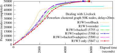
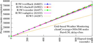
Figure 13: Effectiveness of livelock handling mechanisms. Number of servers=3, number of clients=30. We observed that adaptive mechanism worked best for Social Media Analysis (Figure 13), and backoff mechanism worked best for Weather Monitoring (Figure 13).

From this figure, we observe that the impact of livelocks is not the same in different applications. In particular, for terminating applications like Social Media Analysis, if the livelock issue is ignored, the computation does not terminate. Likewise, computation does not terminate with the mechanism of reordering of remaining tasks upon rollback. This is anticipated, in part, because recurrence of rollback happens in end-stages where the number of remaining tasks is low. On the other hand, for non-terminating application like Weather Monitoring, livelocks do not cause the computation to stall. Except for adaptive consistency, the effectiveness of different livelock handling strategies are almost similar. From Figure 13, we observe that rollback with adaptive consistency works best for terminating applications, and rollback with backoff works best for non-terminating applications. Therefore, we choose these mechanisms to handle livelocks in the detailed analysis of applications in Section 7.6.

7.6 Analysis of Applications

In this section, to illustrate the benefit of our approach, we run the recovery algorithm described in section 6.1 for two applications: Weather Monitoring and Social Media Analysis. We do not consider Conjunctive, as it was designed explicitly to cause too many violations for the purpose of detecting latency of violations. The analysis was performed in our local lab network with the round-trip latency varying between $5\text{\,}\mathrm{ms}50\text{\,}\mathrm{ms}$. We use the approach in Section 7.1 to add additional delays to evaluate the behavior of the application in a realistic setting where replicas are not physically co-located. In order to deal with livelocks, we utilize the backoff mechanism for Weather Monitoring application, and adaptive mechanism for Social Media Analysis application. The number of servers was 3 and the number of clients was 30.

Weather Monitoring. When running the Weather Monitoring application with eventual consistency, first, we consider the nodes organized in a line. In this case, the application progressed $47.2\text{\,}\mathrm{\char 37\relax}$ faster than running on sequential consistency (cf. Figure 14). Even if we extend it to a grid graph, the results are similar. In Figure 14, we find that in the grid graph, the application progressed $46.8\text{\,}\mathrm{\char 37\relax}$ faster under eventual consistency than in sequential consistency. In both of these executions, no violations were detected in the $500\text{\,}\mathrm{s}1,000\text{\,}\mathrm{s}$ window, respectively.

To evaluate the effect of rollbacks, we increase the chance of conflicts by reducing the coverage of each client (i.e. the number of nodes in the graph assigned to each client) so that the clients work on bordering nodes more frequently. In that setting, on a line graph, eventual consistency still progressed about $45\text{\,}\mathrm{\char 37\relax}$ faster than running on sequential consistency (cf. Figure 14), even though we had a substantial number of rollbacks ($36$ in $500\text{\,}\mathrm{s}$). The detection latency for violation was on average $18\text{\,}\mathrm{ms}$. The worst case detection latency was $55\text{\,}\mathrm{ms}$. We note that the application motivated by Weather Monitoring is a non-terminating application which keeps running without termination. Hence, the number of nodes processed measured in stable phase reflects the overall progress of the application. For this reason, in order to compare the progress of different experiment configurations, we measure the progress made by the clients after the same execution duration. For example, in Figure 14, the larger points on each line are where we measure the progress after the execution has run for $490\text{\,}\mathrm{s}$. Figure 14 also considers the progress made by the application on eventual consistency without rollback or monitoring. Thus, the resulting answer may be incorrect. The reason for this analysis is to evaluate the cost of monitoring and rollback. As shown in Figure 14, the cost of rollback is very small. Specifically, with rollback, the number of nodes processed decreased by about $1.4\text{\,}\mathrm{\char 37\relax}$.

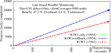
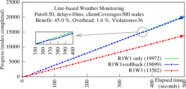
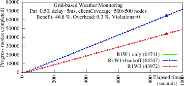
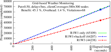
Figure 14: The benefit and overhead of Eventual consistency+Rollback vs. Sequential consistency in Weather Monitoring application. The inset figure within Figure 14 is a close-up view showing the impact of rollback. The larger points near the end of each data sequence are where we choose the representative values for the data sequences.

In grid-based graphs, eventual consistency progressed $45.1\text{\,}\mathrm{\char 37\relax}$ faster than sequential consistency did (cf. Figure 14) even though it had to rollback a number of times (68 times in $1,000\text{\,}\mathrm{s}$). The detection latency was $10\text{\,}\mathrm{ms}$ on average, and $41\text{\,}\mathrm{ms}$ in the worst case. The cost of rollback was $1.4\text{\,}\mathrm{\char 37\relax}$.

Social Media Analysis. Since the Weather Monitoring task is a non-terminating task, its behavior remains the same throughout the execution. Hence, to evaluate the effect of termination, we evaluate our approach in the Social Media Analysis application. Terminating computation suffer from the following when compared with non-terminating computations: (1) At the end, some clients may have completed their task thereby reducing the level of concurrency, and (2) The chance of rollback resulting in the same conflict increases, as the tasks remaining are very small. Therefore, the computation after rollback is more likely to be similar to the one before the rollback. In other words, the conflict is likely to recur.

We evaluate the effect of termination in two types of graph: (1) Power-law clustering (cf. Figure 15), and (2) Regular graphs (cf. Figure 15) where degrees of all nodes are close. (The details of these graphs is given in Section 7.1.)

On power-law clustering graphs, as shown in Figure 15, before the execution reached $90\%$ completion of the work, eventual consistency – even with the cost of monitoring and rolling back – progressed about $18.5\%$ faster than sequential consistency. However, in the remaining $10\%$ of the work, when there were a few nodes to be colored, the chance of conflict increased. Furthermore, the same conflict occurred after rollback as well. Hence, in the final phase, execution under eventual consistency almost stalled due to frequent rollbacks. When the clients utilized adaptive consistency then they could make progress through the final phase and finished about $9.5\%$ faster than sequential consistency. We note that the decline in computation rate in the final phase is also true for sequential consistency, and that is related to a property of power-law cluster graph that some nodes are high degree nodes. In regular random graph, we do not observe this decline as shown in Figure 15. The main reason for this is that the likelihood of conflict in the power-law graph is high since there are several nodes with a high degree. Furthermore, it is difficult to distribute the workload of power-law clustering graph to the clients evenly. Therefore, in the final phase, some clients have completed before the others, thus reducing the parallelism. By contrast, in the regular graph, the likelihood of conflict in end stages remains the same and the workload can be evenly distributed among the clients. On a regular graph, eventual consistency with monitoring and rollback was $26\%$ faster than sequential consistency before $90\%$ of the nodes were processed, and $20.8\%$ faster overall (cf. Figure 15).

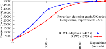
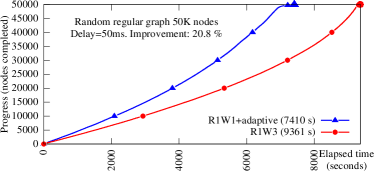
Figure 15: Comparing the completion time of Sequential Consistency (R1W3) vs. Eventual Consistency with rollback and adaptive consistency (R1W1+adaptive) in Social Media Analysis application. On a power-law clustering graph, before 90% of the nodes are processed, R1W1+adaptive progresses about 18% faster than R1W3. Overall, R1W1+adaptive is $9.5\%$ faster than R1W3. On a regular random graph, the benefit before $90\%$ of the nodes are processed is $26\%$ and the overall benefit is $20.8\%$.

7.7 Discussion

In this section, we consider some of the questions raised by this work including questions raised by the reviewers of LADC 2018 and JBCS.

What is the likely effect of the number of clients on the probability of rollback? First, we note that for linear predicates (e.g. conjunctive predicates), when the number of clients increases, the number of violations decreases as it is less likely to find a consistent snapshot where the local predicate at every client is true [33]. As a result, if we increase the concurrency level, the probability of rollback decreases. Hence in the following discussion, we limit the context to semi-linear predicates (e.g. mutual exclusion).

In general, the probability of rollback depends upon the probability that two clients are updating conflicting data. Thus, if the number of clients is too large when compared with the size of the graph (i.e. the coverage of a client is too small), the probability of conflict/rollback is high. We have validated this with experimental analysis of applications motivated by Weather Monitoring in section 7.6. However, in a typical deployment, the coverage of a client is usually large enough (e.g. thousands of nodes) that the chance of two clients concurrently working on neighboring nodes is small. Furthermore, when working on neighboring nodes, clients utilize mutual exclusion mechanism such as Peterson locks to prevent conflicts. Conflicts/rollbacks only happen when there is some data inconsistency related to the mutual exclusion mechanism that causes the clients concurrently updating neighboring nodes. In eventual consistency, data inconsistencies exist but are rare [34] and usually involve hardware and/or network failures. Hence, from our analysis, we anticipate that the probability of rollback is small given that each client is assigned a reasonable workload.

How do the observations in this paper relate to the CAP theorem? When latency increases, we are simulating pseudo network partition. In this case, which consistency level is better depends upon the configuration of the Voldemort servers.

As an illustration, consider the example where we have 5 servers and we use R2W4. Furthermore, suppose that one of the servers is partitioned from the other 4 servers.

With sequential consistency, the 4 servers and their associated clients can still make progress correctly. The partitioned server and its clients would not make progress. Hence, they could be considered as being dead. By some detection mechanism, we can detect such partitioning and assign the tasks of dead clients to other clients. And the computation could progress to the end.

With eventual consistency, all 5 servers and their clients make progress but the clients will process based on stale data. When the network is recovered, the data inconsistencies will invalidate the computation results of both sub-networks. When the monitor detects such partition and inconsistencies, we will have to rollback the whole systems, including the 4 servers and their clients (even though their results are correct, given that the partitioned server has been rolled back).

While the above discussion applies to R2W4, if the system used R1W5 then neither eventual consistency nor sequential consistency could make progress. This is because eventual consistency would result in inconsistently updated replicas. These inconsistencies would be resolved based on the implementation of Voldemort (e.g., latest write wins, minority replicas follow the majority replicas, etc). However, this conflict resolution may not be consistent with the needs of the application. And, in sequential consistency, no write operation would succeed. However, if the nodes are not partitioned but rather suffer from a high delay (but no partition), eventual consistency may be able to make progress. However, it would need to rollback frequently. By contrast, in sequential consistency, it is likely that most write operations fail (as they take too long to complete). Consequently, sequential consistency will not be able to make progress.

What the above discussion suggests is that when the delays are very high, the above approach would work for some configurations (e.g., R2W4) but not for others (e.g. R1W5). Hence, one of the future work in this area is to allow only certain clients to rollback while allowing others to continue without rollback.

Applications that cannot be rolled back. In this paper, we assume the application has exclusive access to its data. Specifically, before the application finishes, other applications will not read this application results. If the data is shared and used by multiple applications, then the rollback approach is not suitable since it is almost impossible to rollback other applications. For instance, the results of computing shortest paths, routing information can be produced by one application and used by other applications. In this case, other approaches such as self-stabilization can be useful.

8 Related Work

8.1 Predicate Detection in Distributed Systems

Predicate detection is an important task in distributed debugging. An algorithm for capturing consistent global snapshots and detecting stable predicates was proposed by Chandy and Lamport [35]. A framework for general predicate detection is introduced by Marzullo and Neiger [18] for asynchronous systems, and Stollers [17] for partially synchronous systems. These general frameworks face the challenge of state explosion as the predicate detection problem is NP-hard in general [14]. However, there exist efficient detection algorithms for several classes of practical predicates such as unstable predicates [36, 22, 37], conjunctive predicates [13, 38], linear predicates, semilinear predicates, bounded sum predicates [14]. Some techniques such as partial-order method [39] and computation slicing [40, 41] are also approaches to address the NP-Completeness of predicate detection. Those works use vector clocks to determine causality and the monitors receive states directly from the constituent processes. Furthermore, the processes are static. [42, 43] address the predicate detection in dynamic distributed systems. However, the class of predicate is limited to the conjunctive predicate. In this paper, our algorithms are adapted for detecting the predicate from only the states of the servers in the key-value store, not from the clients. The servers are static (except failure), but the clients can be dynamics. The predicates supported include linear (including conjunctive) predicates and semilinear predicates.

In [44, 45], the monitors use Hybrid Logical Clock (HLC) to determine causality between events in a distributed execution. HLC has the advantage of low overhead but suffers from false negatives (some valid violations are not detected). In contrast, we use hybrid vector clocks to determine causality in our algorithms. In [33], the authors discussed the impact of various factors, among which is clock synchronization error, on the precision of the monitors. In this paper, we set epsilon at a safe upper bound for practical clock synchronization error to avoid missing potential violations. In other words, a hybrid vector clock is practically a vector clock. Furthermore, this paper focuses on the efficiency and effectiveness of the monitors. Bloom Clock [46] is another alternative to vector clock. Due to the overhead of the counting Bloom filter, the benefit of Bloom clock only payoffs on very large distributed systems.

8.2 Distributed data-stores

Many NoSQL data-stores exist on the market today, and a vast portion of these systems provide eventual consistency. The eventual consistency model is especially popular among key-value and column-family databases. The original Dynamo [1] was one of the pioneers in the eventual consistency movement and served as the basis for Voldemort key-value store. Dynamo introduced the idea of hash-ring for data-sharding and distribution, but unlike Voldemort it relied on server-side replication instead of active client replication. Certain modern databases, such as Cosmos DB and DynamoDB  [47, 48] offer tunable consistency guarantees, allowing operators to balance consistency and performance. This flexibility would enable some applications to take advantage of optimistic execution while allowing other applications to operate under stronger guarantees if needed. However, many data-stores  [49, 50] are designed to provide strong consistency and may not benefit from optimistic execution module.

Aside from general purpose databases, a variety of specialized solutions exist. For instance, TAO  [51] handles social graph data at Facebook. TAO is not strongly consistent, as its main goal is performance and high scalability, even across datacenters and geographical regions. Gorilla  [52] is another Facebook’s specialized store. It operates on performance time-series data and highly tuned for Facebook’s global architecture. Gorilla also favors availability over consistency in regards to the CAP theorem. Crail-KV [53] is Samsung’s extension for Apache Crail data storage system [54] that leverages recent advances in hardware technology, especially key-value solid state drive, to provide higher I/O performance for distributed data store.

Various consistency models in distributed system are presented in the survey [55]. In [56], the authors introduce the notion of Fluctuating Eventual Consistency which is the mix of eventual consistency and strong consistency in order to provide stronger guarantee for eventual consistency. However, this correctness property is not suitable for the adaptive behaviour of application since it is not sufficient to prevent violations as sequential consistency does, and it has more extra synchronization effort than eventual consistency. Consistify [57] is a framework that supports tuning the consistency level of a distributed data store. However, Consistify has to statically analyzes the semantics of the application.

8.3 Snapshots and Reset

The problem of acquiring past snapshots of a system state and rolling back to these snapshots has been studied extensively. Freeze-frame file system  [58] uses Hybrid Logical Clock (HLC) to implement a multi-version Apache HDFS. Retroscope   [11] takes advantage of HLC to find consistent cuts in the system's global state by examining the state-history logs independently on each node of the system. The snapshots produced by Retroscope can later be used for node reset by simple swapping of data-files. Eidetic systems  [59] take a different approach and do not record all prior state changes. Instead, the eidetic system records any non-deterministic changes at the operating system level and constructing a model to navigate deterministic state mutations. This allows the system to revert the state of an entire machine, including the operating system, data and applications, to some prior point. Certain applications may not require past snapshots and instead need to quickly identify consistent snapshots in the presence of concurrent requests affecting the data. VLS  [60] is one such example designed to provide snapshots for data-analytics applications while supporting high throughput of requests executing against the system.

8.4 Distributed Data Processing

MapReduce [61], DataFlow [62] are general-purpose distributed data processing frameworks. In the realm of distributed graph processing, many frameworks are available such as Pregel [63], GraphLab [64], GraphX [65], and PowerGraph [66]. In those works, data is persisted in semi-structural storages such Google File System, Hadoop Distributed File Systems [67], BigTable [68], or in in-memory storage such as Spark [69]. Our work focuses on the no-structure key-value stores and the impact of different consistency models on key-value store performance. Our approach’s usefulness is also not limited to graph applications.

9 Conclusion

Due to limitations of the CAP theorem and the desire to provide availability/good performance during network partitions (or long network delays), many key-value stores choose to provide a weaker consistency such as eventual or causal consistency. This means that the designers need to develop new algorithms that work correctly under such weaker consistency models. An alternative approach is to run the algorithm by ignoring that the underlying system is not sequentially consistent but monitoring it for violations that may affect the application. For example, in the case of graph-based applications (such as those encountered in Weather Monitoring, Social Media Analysis, etc.), each client operates on a subset of nodes in the graph. It is required that two clients do not update two neighboring nodes simultaneously. In this case, the predicate of interest is that the local mutual exclusion is always satisfied.

We demonstrated the usage of this approach in the Voldemort key-value store. We considered two types of predicates: conjunctive predicates and semi-linear predicates (such as that required for local mutual exclusion). We evaluated our approach using Amazon AWS for graph applications motivated by Social Media Analysis and Weather Monitoring. Our approach improved the client throughput performance by $50\%$ – $80\%$. Furthermore, we find that the number of violations of predicates of interest was infrequent. Violations were also detected promptly. When all clients and servers were in the same region, the violations were detected within $50\text{\,}\mathrm{ms}$ whereas if they were in different regions, time for detection was higher. For example, in a network where clients and servers were located in Frankfurt Germany, Ohio USA, and Oregon USA, violations were detected in less than $3\text{\,}\mathrm{s}$. In this context, the time required for a client to work on one task was at least $22\text{\,}\mathrm{s}$ and was on average $45\text{\,}\mathrm{s}$. Thus, detection latency was significantly lower than the time for processing a task.

We developed an efficient rollback algorithm for graph-based applications with the assumption that all violations are detected quickly enough. Our rollback algorithm has mechanisms to handle livelocks (i.e. multiple rollbacks caused by a recurring violation) such as back-off and adaptive consistency where clients switch from eventual consistency to sequential consistency if violations are frequent. We observe that livelocks occur at the end of terminating computation. This is due to the fact that, in a graph processing application, when the computation is about to terminate, there are only a few nodes of the graph that need to be processed. Hence, if a conflict occurs between two clients $C1$ and $C2$, computation after their rollback is likely to have the same conflict again, as each client has only a very small set of nodes to be processed. In this case, without a livelock mechanism, eventual consistency will fail to process all the nodes. Adaptive consistency is also useful in scenarios where the network condition is unstable for an extended period of time. In this case, data inconsistencies are likely to happen and the clients process stale information and produce incorrect results. By switching to sequential consistency, some clients can make progress while some other clients those do not make progress also do not produce conflicting data. Since Voldemort uses active replication (where clients are responsible for replication), such an adaptive approach can be implemented by clients alone without any changes to the underlying server architecture. If passive replication were used, implementation of an adaptive approach would require servers to perform such a change.

We demonstrated the benefit of using eventual consistency with monitoring and rollback. On non-terminating applications such as those motivated by Weather Monitoring, our approach was $45\%$ – $47\%$ faster than running the application on sequential consistency, even occasional rollbacks occurred during the execution. Furthermore, the cost of the monitors and rollback was as low as $1.4\%$. On terminating applications such as those motivated by Social Media Analysis, adaptive consistency is required as eventual consistency fail to process all nodes. For this reason, the overall benefit is reduced. Specifically, when 90% of the nodes were processed, the benefit was $19\%$ – $26\%$. However, since it needed to switch to sequential consistency at the end due to excessive recurring violations, the final benefit was reduced to $10\%$ – $20\%$.

There are several possible future extensions of this work. Currently, the adaptive solution switches from eventual consistency to sequential consistency based on the feedback from monitors. It is possible that the increase in conflicts is temporary due to network issues. When the condition is resumed to normal, it would be beneficial to run in eventual consistency again. However, in sequential consistency, monitors are not required and, thus, there is no feedback mechanism to determine when using eventual consistency is reasonable. One needs to develop new techniques to permit this possibility.

Another issue is that the monitors used in this work suffer from false positives, i.e., they initiate rollback when it was not absolutely necessary. One possible reason for false positives is that the clients, say $C1$ and $C2$, involved in rollback had only read from the key-value store. In this case, one of the clients can continue the execution without rollback. However, in our implementation, as each client rolls back independently, both of them rollback. If this is prevented, it can not only reduce the wasted work, it can also potentially avoid re-occurrence of conflict between $C1$ and $C2$ after rollback. Another reason for false positives is the impedance mismatch in the synchrony assumptions made by the monitors and the applications [33]. In order to reduce or eliminate the false positives, we would have to augment the clients and servers with more information and the monitors would have to examine the candidates more extensively. Consequently, that would increase the cost of monitoring but reduce the need for performing rollback.

The rollback algorithm proposed in this paper is specific for graph-based application and has the assumption on small detection latency. For a general application, we are investigating the possibility of integrating the monitor with Retroscope [11] to automate the rollback and recovery.

Abbreviation

AWS: Amazon Web Service. CAP: CAP theorem, also known as Brewer’s theorem; C=Consistency, A = Availability, P = Partition tolerance. CPU: Central Processing Unit. EC2: Amazon Elastic Compute Cloud. GP2: Amazon General Purpose SSD storage volume. HDFS: Hadoop Distributed File System. HLC: Hybrid Logical Clock. HVC: Hybrid Vector Clock. I/O: Input/Output. JBCS: Journal of the Brazilian Computer Society. LADC: Latin-American Symposium on Dependable Computing. $\mathrm{ms}$: The time unit millisecond. NP in NP-complete and NP-hard: Non-deterministic Polynomial time. $\mathrm{o}\mathrm{p}\mathrm{s}$: Operations per second. $P$: we often denote a predicate as $P$ in this manuscript (this is not an abbreviation). PC: Personal Computer. PT: Physical Time. RAM: Random Access Memory. $\mathrm{s}$: The time unit second. TAO: Facebook’s The Associations and Objects distributed data store. VC: Vector Clock. VLS: Virtual Lightweight Snapshots. XML: Extensible Markup Language.

Availability of data and material

The source code and experimental results supporting the conclusions of this article are at https://doi.org/10.5281/zenodo.3338381.

Competing interests

The authors declare that they have no competing interests.

Author’s contributions

All authors have contributed to the methodological and research aspects of the research. The authors have also read and approved the final manuscript.

Authors’ information

Duong Nguyen, Michigan State University, nguye476@msu.edu; Aleksey Charapko, University at Buffalo, SUNY, acharapk@buffalo.edu; Sandeep S. Kulkarni, Michigan State University, sandeep@cse.msu.edu; Murat Demirbas, University at Buffalo, SUNY, demirbas@buffalo.edu.

Figures

Figure 1: The detect-rollback approach. When the predicate of interest is violated, system state is restored to the most recent consistent snapshot and the computation resumes from there.

Figure 2: An overall framework for optimistic execution in key-value store.

Figure 3: Architecture of predicate detection module.

Figure 4: Example of predicate in XML format. XML specification for $\neg P\equiv(x_{1}=1\land y_{1}=1)\lor z_{2}=1$.

Figure 5: Illustration of candidates sent from a server to monitors. Illustration of candidates sent from a server to monitors corresponding to three conjunctive predicates. If the predicate is semilinear, the candidate is always sent upon a PUT request of relevant variables..

Figure 6: Illustration of causality relation under HVC interval perspective.

Figure 7: Two phases of a task. Two client tasks involved in a violation. Since detection latency is much smaller than the Read phase time, violation will be notified within Read phase of the current task of at least one client..

Figure 8: Simulating network delay using proxies.

Figure 9: Network arrangement with proxies.

Figure 10: Illustration of result stabilization. The Social Media Analysis application is run three times on Amazon AWS with monitoring enabled. Number of servers (N ) = 3. Number of clients per server (C/N ) = 5. Aggregated throughput measured by Social Media Analysis application in three different runs and their average is shown. This average is used to represent the stable value of the application throughput.

Figure 11: The benefit and overhead of monitoring in Social Media Analysis application. (AWS) Social Media Analysis application, 3 servers, 15 clients. Throughput improvement compared to R1W3 and R2W2 is $57\text{\,}\mathrm{\char 37\relax}$ and $78\text{\,}\mathrm{\char 37\relax}$, respectively, and the overhead of running monitors on each consistency setting (the overhead is less than $2\text{\,}\mathrm{\char 37\relax}$.

Figure 12: Benefit and overhead of monitors in Weather Monitoring application. Percentage of PUT requests is $25\text{\,}\mathrm{\char 37\relax}$ and $50\text{\,}\mathrm{\char 37\relax}$. Number of servers=5. Number of clients = 10. Machines are on the AWS North Virginia region but in different availability zones.

Figure 13: Effectiveness of livelock handling mechanisms. Number of servers=3, number of clients=30. We observed that adaptive mechanism worked best for Social Media Analysis (Figure 13), and backoff mechanism worked best for Weather Monitoring (Figure 13)

Figure 14: The benefit and overhead of Eventual consistency+Rollback vs. Sequential consistency in Weather Monitoring application. The inset figure within Figure 14 is a close-up view showing the impact of rollback. The larger points near the end of each data sequence are where we choose the representative values for the data sequences.

Figure 15: Comparing the completion time of Sequential Consistency (R1W3) vs. Eventual Consistency with rollback and adaptive consistency (R1W1+adaptive) in Social Media Analysis application. On a power-law clustering graph, before 90% of the nodes are processed, R1W1+adaptive progresses about 18% faster than R1W3. Overall, R1W1+adaptive is $9.5\%$ faster than R1W3. On a regular random graph, the benefit before $90\%$ of the nodes are processed is $26\%$ and the overall benefit is $20.8\%$.

References

- [1] DeCandia, G., Hastorun, D., Jampani, M., Kakulapati, G., Lakshman, A., Pilchin, A., Sivasubramanian, S., Vosshall, P., Vogels, W.: Dynamo: Amazon’s highly available key-value store. In: Proceedings of Twenty-first ACM SIGOPS Symposium on Operating Systems Principles. SOSP ’07, pp. 205–220. ACM, New York, NY, USA (2007). doi:10.1145/1294261.1294281
- [2] Brewer, E.A.: Towards robust distributed systems (abstract). In: Proceedings of the Nineteenth Annual ACM Symposium on Principles of Distributed Computing. PODC ’00, p. 7. ACM, New York, NY, USA (2000). doi:10.1145/343477.343502
- [3] Gilbert, S., Lynch, N.: Brewer’s conjecture and the feasibility of consistent, available, partition-tolerant web services. SIGACT News 33(2), 51–59 (2002). doi:10.1145/564585.564601
- [4] Du, J., Iorgulescu, C., Roy, A., Zwaenepoel, W.: Gentlerain: Cheap and scalable causal consistency with physical clocks. In: Proceedings of the ACM Symposium on Cloud Computing. SOCC ’14, pp. 4–1413. ACM, New York, NY, USA (2014). doi:10.1145/2670979.2670983
- [5] Lloyd, W., Freedman, M.J., Kaminsky, M., Andersen, D.G.: Don’t settle for eventual: Scalable causal consistency for wide-area storage with cops. In: Proceedings of the Twenty-Third ACM Symposium on Operating Systems Principles. SOSP ’11, pp. 401–416. ACM, New York, NY, USA (2011). doi:10.1145/2043556.2043593
- [6] Roohitavaf, M., Demirbas, M., Kulkarni, S.S.: Causalspartan: Causal consistency for distributed data stores using hybrid logical clocks. In: 36th IEEE Symposium on Reliable Distributed Systems, SRDS 2017, Hongkong, China, September 26 - 29, 2017, pp. 184–193 (2017)
- [7] Lakshman, A., Malik, P.: Cassandra: a decentralized structured storage system. ACM SIGOPS Operating Systems Review 44(2), 35–40 (2010)
- [8] Project Voldemort. http://www.project-voldemort.com/voldemort/quickstart.html. Accessed: 2019-07-14
- [9] Sumbaly, R., Kreps, J., Gao, L., Feinberg, A., Soman, C., Shah, S.: Serving large-scale batch computed data with project voldemort. In: Proceedings of the 10th USENIX Conference on File and Storage Technologies, pp. 18–18 (2012). USENIX Association
- [10] Brzezinski, J., Wawrzyniak, D.: Consistency requirements of peterson’s algorithm for mutual exclusion of N processes in a distributed shared memory system. In: Proceedings of the International Conference on Parallel Processing and Applied Mathematics-Revised Papers. PPAM ’01, pp. 202–209. Springer, London, UK, UK (2002)
- [11] Charapko, A., Ailijiang, A., Demirbas, M., Kulkarni, S.: Retrospective lightweight distributed snapshots using loosely synchronized clocks. In: Distributed Computing Systems (ICDCS), 2017 IEEE 37th International Conference On, pp. 2061–2066 (2017). IEEE
- [12] Garg, V.K.: Principles of Distributed Systems. Kluwer, Norwell, MA (1996)
- [13] Garg, V.K., Chase, C.M.: Distributed algorithms for detecting conjunctive predicates. In: Distributed Computing Systems, 1995., Proceedings of the 15th International Conference On, pp. 423–430 (1995). IEEE
- [14] Chase, C.M., Garg, V.K.: Detection of global predicates: Techniques and their limitations. Distributed Computing 11(4), 191–201 (1998)
- [15] Nguyen, D.: Supplementary dataset and source code for the paper ”Using Weaker Consistency Models with Monitoring and Recovery for Improving Performance of Key-Value Stores” (2019). doi:10.5281/zenodo.3338381. https://doi.org/10.5281/zenodo.3338381
- [16] Lamport, L.: Time, clocks, and the ordering of events in a distributed system. Commun. ACM 21(7), 558–565 (1978). doi:10.1145/359545.359563
- [17] Stoller, S.D.: Detecting global predicates in distributed systems with clocks. Distributed Computing 13(2), 85–98 (2000)
- [18] Marzullo, K., Neiger, G.: Detection of global state predicates. In: International Workshop on Distributed Algorithms, pp. 254–272 (1991). Springer
- [19] Fidge, C.J.: Timestamps in message-passing systems that preserve the partial ordering (1987)
- [20] Mattern, F.: Virtual time and global states of distributed systems. Parallel and Distributed Algorithms 1(23), 215–226 (1989)
- [21] Demirbas, M., Kulkarni, S.: Beyond truetime: Using augmentedtime for improving google spanner. In: Workshop on Large-Scale Distributed Systems and Middleware (LADIS) (2013)
- [22] Garg, V.K., Waldecker, B.: Detection of weak unstable predicates in distributed programs. IEEE Transactions on Parallel and Distributed Systems 5(3), 299–307 (1994)
- [23] Nguyen, D.N., Kulkarni, S.S., Datta, A.K.: Benefit of self-stabilizing protocols in eventually consistent key-value stores: a case study. In: Proceedings of the 20th International Conference on Distributed Computing and Networking, ICDCN 2019, Bangalore, India, January 04-07, 2019, pp. 148–157 (2019). doi:10.1145/3288599.3288609
- [24] Bovy, C., Mertodimedjo, H., Hooghiemstra, G., Uijterwaal, H., Van Mieghem, P.: Analysis of end-to-end delay measurements in internet. In: Proc. of the Passive and Active Measurement Workshop-PAM, vol. 2002 (2002). sn
- [25] NIST/SEMATECH e-Handbook of Statistical Methods. http://www.itl.nist.gov/div898/handbook/eda/section3/eda366b.htm. Accessed: 2019-07-14 (2013)
- [26] Overview of NetworkX. http://https://networkx.github.io/documentation/stable/. Accessed: 2019-03-24
- [27] Raynal, M.: Distributed Algorithms for Message-passing Systems. Springer, New York (2013)
- [28] Fjukstad, B., Bjørndalen, J.M., Anshus, O.: Embarrassingly distributed computing for symbiotic weather forecasts. Procedia Computer Science 18, 1217–1225 (2013)
- [29] Prakash, R., Shivaratri, N.G., Singhal, M.: Distributed dynamic channel allocation for mobile computing. In: Proceedings of the Fourteenth Annual ACM Symposium on Principles of Distributed Computing, pp. 47–56 (1995). ACM
- [30] Núnez-Rodrıguez, Y., Xiao, H., Islam, K., Alsalih, W.: A distributed algorithm for computing voronoi diagram in the unit disk graph model. In: Proc. 20th Canadian Conference in Computational Geometry (CCCG’08), pp. 199–202 (2008)
- [31] Ranger, C., Raghuraman, R., Penmetsa, A., Bradski, G., Kozyrakis, C.: Evaluating mapreduce for multi-core and multiprocessor systems. In: High Performance Computer Architecture, 2007. HPCA 2007. IEEE 13th International Symposium On, pp. 13–24 (2007). Ieee
- [32] Blanas, S., Patel, J.M., Ercegovac, V., Rao, J., Shekita, E.J., Tian, Y.: A comparison of join algorithms for log processing in mapreduce. In: Proceedings of the 2010 ACM SIGMOD International Conference on Management of Data, pp. 975–986 (2010). ACM
- [33] Yingchareonthawornchai, S., Nguyen, D., Valapil, V.T., Kulkarni, S.S., Demirbas, M.: Precision, recall, and sensitivity of monitoring partially synchronous distributed systems. In: Runtime Verification, pp. 20–30 (2016). Springer
- [34] DeCandia, G., Hastorun, D., Jampani, M., Kakulapati, G., Lakshman, A., Pilchin, A., Sivasubramanian, S., Vosshall, P., Vogels, W.: Dynamo: amazon’s highly available key-value store. ACM SIGOPS operating systems review 41(6), 205–220 (2007)
- [35] Chandy, K.M., Lamport, L.: Distributed snapshots: Determining global states of distributed systems. ACM Trans. Comput. Syst. 3(1), 63–75 (1985). doi:10.1145/214451.214456
- [36] Garg, V.K., Waldecker, B.: Detection of unstable predicates in distributed programs. In: International Conference on Foundations of Software Technology and Theoretical Computer Science, pp. 253–264 (1992). Springer
- [37] Garg, V.K., Waldecker, B.: Detection of strong unstable predicates in distributed programs. IEEE Transactions on Parallel and Distributed Systems 7(12), 1323–1333 (1996)
- [38] Garg, V.K., Chase, C.M., Mitchell, J.R., Kilgore, R.: Conjunctive predicate detection. In: Proceedings Hawaii International Conference on System Sciences HICSS95 (January 1995), IEEE Computer Society (1995). Citeseer
- [39] Stoller, S.D., Unnikrishnan, L., Liu, Y.A.: Efficient detection of global properties in distributed systems using partial-order methods. In: International Conference on Computer Aided Verification, pp. 264–279 (2000). Springer
- [40] Mittal, N., Garg, V.K.: Techniques and applications of computation slicing. Distributed Computing 17(3), 251–277 (2005)
- [41] Chauhan, H., Garg, V.K., Natarajan, A., Mittal, N.: A distributed abstraction algorithm for online predicate detection. In: 2013 IEEE 32nd International Symposium on Reliable Distributed Systems, pp. 101–110 (2013). IEEE
- [42] Wang, X., Mayo, J., Hembroff, G., Gao, C.: Detection of conjunctive stable predicates in dynamic systems. In: Parallel and Distributed Systems (ICPADS), 2009 15th International Conference On, pp. 828–835 (2009). IEEE
- [43] Wang, X., Mayo, J., Hembroff, G.C.: Detection of a weak conjunction of unstable predicates in dynamic systems. In: Parallel and Distributed Systems (ICPADS), 2010 IEEE 16th International Conference On, pp. 338–346 (2010). IEEE
- [44] Valapil, V.T., Kulkarni, S.S.: Biased clocks: A novel approach to improve the ability to perform predicate detection with O(1) clocks. In: Structural Information and Communication Complexity - 25th International Colloquium, SIROCCO 2018, Ma’ale HaHamisha, Israel, June 18-21, 2018, Revised Selected Papers, pp. 345–360 (2018)
- [45] Valapil, V.T., Yingchareonthawornchai, S., Kulkarni, S.S., Torng, E., Demirbas, M.: Monitoring partially synchronous distributed systems using SMT solvers. In: Runtime Verification - 17th International Conference, RV 2017, Seattle, WA, USA, September 13-16, 2017, Proceedings, pp. 277–293 (2017)
- [46] Ramabaja, L.: The bloom clock. CoRR abs/1905.13064 (2019). 1905.13064
- [47] Azure Cosmos DB – Globally Distributed Database Service. https://azure.microsoft.com/en-us/services/cosmos-db/?v=17.45b. Accessed: 2017-12-10
- [48] Amazon DynamoDB – a Fast and Scalable NoSQL Database Service Designed for Internet Scale Applications. http://www.allthingsdistributed.com/2012/01/amazon-dynamodb.html. Accessed: 2017-12-10
- [49] Corbett, J.C., Dean, J., Epstein, M., Fikes, A., Frost, C., Furman, J.J., Ghemawat, S., Gubarev, A., Heiser, C., Hochschild, P., et al.: Spanner: Google’s globally distributed database. ACM Transactions on Computer Systems (TOCS) 31(3), 8 (2013)
- [50] Chang, F., Dean, J., Ghemawat, S., Hsieh, W.C., Wallach, D.A., Burrows, M., Chandra, T., Fikes, A., Gruber, R.E.: Bigtable: A distributed storage system for structured data. ACM Transactions on Computer Systems (TOCS) 26(2), 4 (2008)
- [51] Bronson, N., Amsden, Z., Cabrera, G., Chakka, P., Dimov, P., Ding, H., Ferris, J., Giardullo, A., Kulkarni, S., Li, H.C., et al.: Tao: Facebook’s distributed data store for the social graph. In: USENIX Annual Technical Conference, pp. 49–60 (2013)
- [52] Pelkonen, T., Franklin, S., Teller, J., Cavallaro, P., Huang, Q., Meza, J., Veeraraghavan, K.: Gorilla: A fast, scalable, in-memory time series database. Proceedings of the VLDB Endowment 8(12), 1816–1827 (2015)
- [53] Bisson, T., Chen, K., Choi, C., Balakrishnan, V., Kee, Y.: Crail-kv: A high-performance distributed key-value store leveraging native kv-ssds over nvme-of. In: 2018 IEEE 37th International Performance Computing and Communications Conference (IPCCC), pp. 1–8 (2018). doi:10.1109/PCCC.2018.8710776
- [54] Stuedi, P., Trivedi, A., Pfefferle, J., Stoica, R., Metzler, B., Ioannou, N., Koltsidas, I.: Crail: A high-performance I/O architecture for distributed data processing. IEEE Data Eng. Bull. 40(1), 38–49 (2017)
- [55] Aldin, H.N.S., Deldari, H., Moattar, M.H., Ghods, M.R.: Consistency models in distributed systems: A survey on definitions, disciplines, challenges and applications. CoRR abs/1902.03305 (2019)
- [56] Kokocinski, M., Kobus, T., Wojciechowski, P.T.: On mixing eventual and strong consistency: Bayou revisited. CoRR abs/1905.11762 (2019)
- [57] Sidhanta, S., Mukhopadhyay, S., Golab, W.: Consistify: Preserving correctness and sla under weak consistency. In: Proceedings of the 20th International Conference on Distributed Computing and Networking. ICDCN ’19, pp. 282–291. ACM, New York, NY, USA (2019). doi:10.1145/3288599.3288630. http://doi.acm.org/10.1145/3288599.3288630
- [58] Song, W., Gkountouvas, T., Birman, K., Chen, Q., Xiao, Z.: The freeze-frame file system. In: SoCC, pp. 307–320 (2016)
- [59] Devecsery, D., Chow, M., Dou, X., Flinn, J., Chen, P.M.: Eidetic systems. In: 11th USENIX Symposium on Operating Systems Design and Implementation (OSDI 14), pp. 525–540 (2014)
- [60] Chirigati, F., Siméon, J., Hirzel, M., Freire, J.: Virtual lightweight snapshots for consistent analytics in nosql stores. In: Data Engineering (ICDE), 2016 IEEE 32nd International Conference On, pp. 1310–1321 (2016). IEEE
- [61] Dean, J., Ghemawat, S.: Mapreduce: simplified data processing on large clusters. Communications of the ACM 51(1), 107–113 (2008)
- [62] Akidau, T., Bradshaw, R., Chambers, C., Chernyak, S., Fernández-Moctezuma, R.J., Lax, R., McVeety, S., Mills, D., Perry, F., Schmidt, E., et al.: The dataflow model: a practical approach to balancing correctness, latency, and cost in massive-scale, unbounded, out-of-order data processing. Proceedings of the VLDB Endowment 8(12), 1792–1803 (2015)
- [63] Malewicz, G., Austern, M.H., Bik, A.J., Dehnert, J.C., Horn, I., Leiser, N., Czajkowski, G.: Pregel: a system for large-scale graph processing. In: Proceedings of the 2010 ACM SIGMOD International Conference on Management of Data, pp. 135–146 (2010). ACM
- [64] Low, Y., Bickson, D., Gonzalez, J., Guestrin, C., Kyrola, A., Hellerstein, J.M.: Distributed graphlab: a framework for machine learning and data mining in the cloud. Proceedings of the VLDB Endowment 5(8), 716–727 (2012)
- [65] Gonzalez, J.E., Xin, R.S., Dave, A., Crankshaw, D., Franklin, M.J., Stoica, I.: Graphx: Graph processing in a distributed dataflow framework. In: OSDI, vol. 14, pp. 599–613 (2014)
- [66] Gonzalez, J.E., Low, Y., Gu, H., Bickson, D., Guestrin, C.: Powergraph: distributed graph-parallel computation on natural graphs. In: OSDI, vol. 12, p. 2 (2012)
- [67] Ghemawat, S., Gobioff, H., Leung, S.: The google file system. In: Proceedings of the 19th ACM Symposium on Operating Systems Principles 2003, SOSP 2003, Bolton Landing, NY, USA, October 19-22, 2003, pp. 29–43 (2003)
- [68] Chang, F., Dean, J., Ghemawat, S., Hsieh, W.C., Wallach, D.A., Burrows, M., Chandra, T., Fikes, A., Gruber, R.E.: Bigtable: A distributed storage system for structured data. ACM Transactions on Computer Systems (TOCS) 26(2), 4 (2008)
- [69] Zaharia, M., Chowdhury, M., Das, T., Dave, A., Ma, J., McCauley, M., Franklin, M.J., Shenker, S., Stoica, I.: Resilient distributed datasets: A fault-tolerant abstraction for in-memory cluster computing. In: Proceedings of the 9th USENIX Conference on Networked Systems Design and Implementation, pp. 2–2 (2012). USENIX Association