Chiral Waves on the Fermi-Dirac Sea:
Quantum Superfluidity and the Axial Anomaly

Abstract

We show that as a result of the axial anomaly, massless fermions at zero temperature define a relativistic quantum superfluid. The anomaly pole implies the existence of a gapless Chiral Density Wave (CDW), i.e. an axion-like acoustic mode of an irrotational and dissipationless Hamiltonian perfect fluid, that is a correlated fermion/anti-fermion pair excitation of the Fermi-Dirac sea. In $D\!=\!2$ dimensions the chiral superfluid effective action coincides with that of the Schwinger model as $e\rightarrow 0$, and the CDW acoustic mode is precisely the Schwinger boson. Since this identity holds also at zero chiral chemical potential, the Dirac vacuum itself may be viewed as a quantum superfluid state. The CDW collective boson is a $U(1)$ chiral phase field, which is gapless as a result of a novel, non-linear realization of Goldstone’s theorem, extended to this case of symmetry breaking by an anomaly. A new local form of the axial anomaly bosonic effective action in any $D$ even spacetime is given, consistent with superfluidity, and its quantization is shown to be required by the anomalous Schwinger terms in fermion current commutators. In QED₄ this collective Goldstone mode appears as a massless pole in the axial anomaly triangle diagram, and is responsible for the macroscopic non-dissipative currents of the Chiral Magnetic and Chiral Separation Effects, as well as the Anomalous Hall Effect. In a constant uniform magnetic field an exact dimensional reduction from $D\!=\!4$ to $D\!=\!2$ occurs and the collective $e^{+}e^{-}$ CDW chiral pair excitation propagating along the magnetic field direction is a Chiral Magnetic Wave, which acquires a mass gap $M^{2}\!=\!e^{3}B/2\pi^{2}$. Possible realizations and tests of the theory of collective bosonic excitations due to the anomaly in Dirac/Weyl materials are briefly discussed.

I Introduction

The derivation of macroscopic fluid hydrodynamics from microscopic quantum field theory is of fundamental importance, underlying many branches of physics. This is a formidable problem in general, spanning a very large range of scales. The relationship between the macroscopic and microscopic realms becomes more immediate at very low temperatures, approaching absolute zero, where quantum behavior dominates, and can be responsible for long range collective phenomena.

An example of this closer connection at low temperatures and finite densities is provided by macroscopic superfluid behavior, characterized experimentally by persistent, non-dissipative currents and gapless sound modes Khalatnikov (2000). Theoretically these striking features are consequences of the spontaneous breaking of the continuous global $U(1)$ phase symmetry associated with the conservation of particle number, and the formation of a macroscopic coherent condensate exhibiting off-diagonal long range order Penrose (1951); Penrose and Onsager (1956); Yang (1962); Brown (1992). The $U(1)$ phase is a field describing an acoustic density wave excitation that is identified as a gapless Nambu-Goldstone boson Nambu and Jona-Lasinio (1961a); Goldstone (1961); Goldstone et al. (1962). Although condensation to a superfluid state is a property of systems obeying Bose statistics, fermions such as ³He can form Cooper pairs that act as effective bosons which condense and also form superfluids Giorgini et al. (2008).

Our first purpose in this paper is to show that the macroscopic properties of a relativistic superfluid are satisfied in fundamental theories such as quantum electrodynamics (QED), with weakly interacting massless fermions that possess an anomaly in their axial currents $\tilde{J}^{\lambda}=\bar{\psi}\gamma^{\lambda}\gamma_{{}_{D+1}}\psi$, when coupled to an external gauge potential $A_{\lambda}$. Here $\gamma_{{}_{D+1}}$ is the Dirac chirality matrix equal to $\gamma_{5}$ in $D\!=\!4$ dimensions, defined in general even $D$ by eq. (114), and the chiral current $\tilde{J}^{\lambda}$ is the Noether current corresponding to the global $U^{ch}(1)$ chiral rotation $\psi\rightarrow e^{i\alpha\gamma_{{}_{D+1}}}\,\psi$ of the Dirac fermion field, which rotates left and right handed fermions by an opposite phase.

In $D\!=\!2$ spacetime ($d\!=\!1$ space) dimensions we prove that the relationship between quantum superfluidity and massless fermion QED₂ is an identity. In fact, the effective action of the superfluid description coincides with that of the bosonized Schwinger model of massless QED₂ Schwinger (1962) in the limit of vanishingly small electric charge coupling $e\!\to\!0$. In other words, in this case at least, macroscopic fluid behavior is directly derivable from the microscopic theory, and the axial anomaly is the bridge spanning scales that makes this connection possible. At non-zero chiral density $\tilde{n}$, and chemical potential $\tilde{\mu}$, the axial anomaly necessarily leads to a propagating Chiral Density Wave (CDW), which is a bosonic collective mode comprised of fermion/hole pair excitation of the Fermi sea.

The fact that $D\!=\!2$ fermions form a (Luttinger) liquid with a bosonized CDW has been anticipated Haldane (1981). However, the relation to the Schwinger model, the essential role of its axial anomaly and precise identification with the anomalous chiral superfluid effective action has not been demonstrated previously. More remarkable still, since the superfluid acoustic mode depends only upon the ratio $\tilde{\mu}/\tilde{n}=\pi$, which is a fixed constant for free fermions in $D\!=\!2$, the superfluid description extends also to limiting case of $\tilde{\mu}=\pi\tilde{n}\rightarrow 0$, in which case the CDW becomes a fermion/anti-fermion pair excitation of the Dirac sea, implying that the Dirac vacuum itself may also be regarded as a kind of superfluid state. This is demonstrated in Secs. II-III. To our knowledge this is the first instance in which a connection between macroscopic superfluid behavior and the microscopic quantum fermion vacuum has been rigorously established.

The existence of a gapless collective boson CDW arising from the axial anomaly immediately raises a second fundamental question, namely the applicability of Goldstone’s theorem. In the more familiar case of Spontaneous Symmetry Breaking (SSB), the vacuum or low temperature ground state of the system is described by a scalar order parameter, namely the expectation value $\langle\Phi\rangle$ which is non-invariant under a $U(1)$ global symmetry at the minimum of an effective potential Schmitt (2015), but the Ward Identities are exactly preserved. A massless Goldstone boson then follows in dimensions $D\!>\!2$ Brown (1992). This is in contrast to symmetry breaking by the fermionic axial anomaly – Anomalous Symmetry Breaking (ASB) – where the naive chiral Ward Identities are explicitly violated Adler (1969); Treiman et al. (1972); Bertlmann (1996), and there is no readily apparent effective potential to be minimized for a scalar order parameter. The standard form of Goldstone’s theorem does not obviously apply to this case, and the origin of the gapless bosonic excitation in fermionic ASB therefore is more subtle.

That a gapless boson is implied by the anomaly was first recognized in the anomalous triangle diagram of massless QED in $D\!=\!4$ by a dispersive approach, as an infrared singularity, independent of any ultraviolet (UV) regularization Dolgov and Zakharov (1971). General arguments of analyticity and unitarity lead to the same conclusion Frishman et al. (1981); Coleman and Grossman (1982), linking short distance to long distance behavior by the ‘t Hooft consistency condition ‘t Hooft (1980), and the Adler-Bardeen theorem Adler and Bardeen (1969). In Refs. Giannotti and Mottola (2009) and Blaschke et al. (2014) it was demonstrated that the massless boson pole of the axial anomaly in both $D\!=\!2$ and $D\!=\!4$ dimensions arises from correlated pairs of massless fermions and anti-fermions (particle-hole pairs in the condensed matter context) traveling together co-linearly at the speed of light. In other words, the axial anomaly itself implies fermion pairing and the existence of a propagating gapless effective boson excitation, analogous to Cooper pairing, even in the limit of very weak (or in the limiting case of absence of) fermion self-interactions. This gapless excitation is made explicit in $D\!=\!2$ by the techniques of bosonization Coleman (1975). In $D\!=\!4$ a bosonic form of the effective action of the axial anomaly was given in Giannotti and Mottola (2009). It has become recognized only relatively recently that the appearance of a collective massless boson mode, not apparent in the classical Lagrangian, is a general feature of both axial and conformal anomalies, whose effects can extend to long distance or macroscopic scales Mottola and Vaulin (2006); Armillis et al. (2010); Mottola (2010). Since the distinguishing feature of SSB, a gapless excitation, is present in massless fermion theories with an axial anomaly, it suggests that Goldstone’s theorem can be generalized and extended to anomalous fermion theories, despite there being no effective potential or scalar order parameter immediately apparent at the outset.

Demonstrating that Goldstone’s theorem can indeed be generalized to ASB is our second main purpose in this paper. The novel extension of Goldstone’s theorem in the case of ASB differs from SSB in that it rests upon the anomalous current commutators, or Schwinger terms, in the underlying fermion theory, which remain non-vanishing even in the weak coupling limit $e\!\to\!0$ and vanishing background gauge field, where the divergence $\partial_{\lambda}\tilde{J}^{\lambda}=\bar{\psi}\gamma^{\lambda}\gamma_{{}_{D+1}}\psi\to 0$. In this limit there is a propagating (pseudo-)scalar CDW, and this bosonic collective mode is associated with fermion condensation and $\langle\bar{\psi}\psi\rangle\neq 0$. This extension of Goldstone’s Theorem to ASB is proven in Sec. IV.

The weak coupling limit $e\!\rightarrow\!0$ is subtle, particularly in $D\!=\!2$ dimensions, where the Mermin-Wagner-Coleman (MWC) theorem Mermin and Wagner (1966); Coleman (1973) tells us that there can be no true long-range order and no true Goldstone bosons. The $D\!=\!2$ case therefore merits special attention. Since the would-be Goldstone mode is just the boson of the Schwinger model in $D\!=\!2$, it becomes massive or gapped with $M^{2}=e^{2}/\pi$, so that for any finite $e$, however small, the Goldstone mode becomes ‘Higgsed,’ there is no long range order and no gapless mode at distances greater than $1/M$, consistent with the MWC theorem. Nevertheless as $e\!\to\!0$ but $L\to\infty$ with $eL\gtrsim 1$ fixed, the CDW approximates a Goldstone mode over a larger and larger range of distance scales with only algebraic power law decay of the correlator. This is the behavior known as ‘quasi-long-range order’ Sachdev (2011).

The third major goal of this paper is to extend the derivation of macroscopic behavior from quantum field theory to higher (even) dimensions larger than two, again relying upon the axial anomaly and the anomaly pole. We show in Sec. V that bosonization and macroscopic superfluidity effects persist in higher dimensions as well, as a direct result of the axial anomaly, at least at $T\!=\!0$ for massless fermions, in a subsector of the theory at weak enough coupling that self-interactions can be neglected. This relies upon a new form of the effective bosonic action of the axial anomaly in any $D\!=2n$ even dimensions in the longitudinal sector of the axial current, where the massless boson anomaly pole of the triangle $\langle\tilde{J}^{\lambda}J^{\alpha}J^{\beta}\rangle$ diagram resides. This collective boson in $D\!=\!4$, again composed of massless fermion pairs, is entirely responsible for the non-dissipative, macroscopic Chiral Magnetic and Chiral Separation currents of QED₄ Kharzeev et al. (2016); Huang (2016). That the same $D\!=\!4$ effective action and massless pole of the triangle anomaly of QED₄ is also responsible for the Anomalous Hall Effect in quantum materials such as Weyl semi-metals Landsteiner (2016) is shown in Sec. V.4, in another example of a macroscopic quantum effect in $D>2$ directly traceable to the microscopic anomaly.

In the case of a constant and uniform magnetic field $\boldsymbol{B}$ background with a parallel $\boldsymbol{E}$ field independent of the transverse coordinates, the $D\!=\!4$ triangle anomaly reduces to the $D\!=\!2$ case. The CDW along the common $\boldsymbol{E}\parallel\boldsymbol{B}$ direction is a Chiral Magnetic Wave (CMW), coinciding with the Schwinger boson collective excitation in $D\!=\!2$; or in other words this is an example of dimensional reduction, where macroscopically observable quantum coherence effects resulting from the microscopic QFT anomaly in $D>2$ dimensions can be rigorously related back to the $D\!=\!2$ case. The role of the dimensionful $D\!=\!2$ coupling of the Schwinger model is taken by $2\alpha eB$. This is also a new result, rigorously proven for the first time to our knowledge in Sec. VI.

As a final example of macroscopic effects in $D\!=\!4$, we consider in Sec. VII free massless fermions at finite chiral density in QED₄, where the collective boson predicted by the Goldstone theorem extended to ASB of Sec. IV is a gapless acoustic mode propagating at the sound speed $v_{s}^{2}=\frac{dp}{d\varepsilon}=\frac{1}{3}$, sourced by and coupled to $\boldsymbol{E}\cdot\boldsymbol{B}$. Possible realizations of the CDW as an axion-like mode in Weyl materials are briefly discussed in Sec. VIII, in the Summary and Outlook.

There are three Appendices containing some additional technical details, included for completeness and supplementing the main text. Appendix A clarifies the relationship between the superfluid energy-momentum tensor and Hamiltonian. Appendix B collects a number of useful formulae for free fermions in two dimensions and their bosonization for reference. Appendix C examines the delicate limit of $e\to 0$ in a finite volume system in $D\!=\!2$, the $\theta$-vacuum periodicity arising from topologically non-trivial gauge transformations, and fate of the Nambu-Goldstone mode in the Schwinger model in the infinite spatial volume limit.

Note on Organization of the Paper:

In the interest of making the paper as self-contained and accessible to as wide a cross-disciplinary audience as possible, review of some topics, such as the Schwinger model and triangle anomaly seemed necessary, particularly since they may not be familiar to readers with different backgrounds. For the most part this supplementary review material is relegated to the Appendices. A Table of Contents and brief account of the main new results and their importance are provided both in this Introduction, and summarized again in Sec. VIII, with references to the specific numbered relations establishing these results in the text, for the convenience of readers who may wish to skip directly to those sections containing the results in which they are most interested.

II Ideal Hydrodynamics of An Anomalous Chiral Fluid

II.1 Euler-Lagrange Action Principle

We begin by giving the action principle that provides a consistent framework for relativistic ideal chiral fluids incorporating the axial anomaly. This is a new gauge invariant formulation which unlike some earlier treatments, e.g. Monteiro et al. (2015), conserves electric charge. It extends and generalizes earlier discussions of relativistic but non-anomalous or non-chiral fluids Schutz (1970); Jackiw et al. (2004). Those were based on generalizing to Lorentz invariant systems the Euler-Lagrange action principle for non-relativistic fluids Clebsch (1859). The key ingredient of these variational principles is the introduction of a ‘dynamic velocity’ vector field $\boldsymbol{\xi}$ that can be expressed in terms of scalar (Clebsch) potentials Seliger and Whitham (1968). In its relativistic generalization the dynamic velocity $\xi_{\lambda}$ is a covariant $D$-vector in $D$ spacetime dimensions that couples to the conserved current whose hydrodynamic flow is under study. In this paper the fermionic axial current $\tilde{J}^{\lambda}=\bar{\psi}\gamma^{\lambda}\gamma_{{}_{D+1}}\psi$ is our primary focus.

In general several Clebsch potentials, denoted by $\eta,\alpha,\beta,\dots$ are necessary to describe arbitrary rotational motions of a fluid and entropy flow at finite temperatures, in terms of which the dynamic velocity can be expressed as $\xi_{\lambda}=-\partial_{\lambda}\eta+\alpha\,\partial_{\lambda}\beta+\dots$Schutz (1970). However the essential feature of a superfluid is that it should be dissipationless. This implies that the $\alpha,\beta,\dots$ terms describing entropy or rotational currents are negligible, and should vanish entirely at zero temperature. In that case the dynamic velocity field can be expressed as a pure gradient of a single scalar potential to be denoted here by $\eta$, so that we may take $\xi_{\lambda}=-\partial_{\lambda}\eta$. Then the minimal action for ideal hydrodynamics of a chiral superfluid in $D=d+1$ (even) spacetime dimensions is

$$S_{\chi\rm fl}=\int\!\!d^{D}\!x\,{\cal L}_{\chi\rm fl}=\int\!\!d^{D}\!x\left\{\big{(}\partial_{\lambda}\eta+\tilde{A}_{\lambda}\big{)}\tilde{J}^{\lambda}+\eta\,{{\mathscr{A}}}_{D}\!-\!\varepsilon(\tilde{n})\right\}$$ (1)

where the tildes denote chiral quantities, $\tilde{n}$ is the chiral number density and $\varepsilon(\tilde{n})$ is the equilibrium energy density of the fluid in its rest frame. An external axial potential $\tilde{A}_{\lambda}$ is introduced so that

$$\frac{\delta S_{\chi\rm sf}}{\delta\tilde{A}_{\lambda}}=\tilde{J}^{\lambda}=\tilde{n}\,u^{\lambda}$$ (2)

is defined, with $u^{\lambda}$ the relativistic kinetic velocity of the fluid. Since the relativistic velocity is normalized by $u^{\lambda}u_{\lambda}=u^{\lambda}g_{\lambda\nu}u^{\nu}=-1$ in units in which the speed of light $c=1$, with $g_{\lambda\nu}$ the spacetime metric, the chiral number density can be expressed in the relativistically invariant form

$$\tilde{n}\equiv\left(-\tilde{J}^{\lambda}\tilde{J}_{\lambda}\right)^{\frac{1}{2}}$$ (3)

in terms of the axial current. The ${{\mathscr{A}}}_{D}$ term takes account of the axial current anomaly in (4) below. For some related discussions of effective actions for anomalous fluids, see Lublinsky and Zahed (2010); Dubovsky et al. (2014); Monteiro et al. (2015); Glorioso et al. (2019).

The variational principle for the fluid action (1) requires that the pseudoscalar Clebsch potential $\eta$ and the axial current $\tilde{J}^{\lambda}$ be varied independently, in addition to the variation (2). Variation of (1) with respect to $\eta$ gives

$$\partial_{\lambda}\tilde{J}^{\lambda}={\mathscr{A}}_{D}\stackrel{{\scriptstyle D=2n}}{{=}}\frac{2}{(4\pi)^{n}\,n!}\,\epsilon^{\mu_{1}\nu_{1}...\mu_{n}\nu_{n}}F_{\mu_{1}\nu_{1}}...F_{\mu_{n}\nu_{n}}$$ (4)

where ${\mathscr{A}}_{D}$ is the axial anomaly for massless Dirac fermions, $F_{\mu\nu}=\partial_{\mu}A_{\nu}-\partial_{\nu}A_{\mu}$ is the electromagnetic field strength, and $\epsilon^{\mu_{1}\nu_{1}...\mu_{n}\nu_{n}}$ is the totally anti-symmetric Levi-Civita tensor in $D\!=\!2n$ even dimensions Zumino et al. (1984). We focus on the $D=2,4$ cases explicitly in this paper, providing a basis for the superfluid action (1) from QFT first principles, by which $\eta$ will be identified with the dynamical phase field of chiral symmetry breaking.

Variation of (1) with respect to the axial current $\tilde{J}^{\lambda}$ gives

$$\frac{\delta}{\delta\tilde{J}^{\lambda}}S_{\chi\rm fl}=\partial_{\lambda}\eta+\tilde{A}_{\lambda}-\left(\frac{d\varepsilon}{\,d\tilde{n}}\right)\left(\frac{d\tilde{n}}{d\tilde{J}^{\lambda}}\right)=\partial_{\lambda}\eta+\tilde{A}_{\lambda}+\mbox{\small$\displaystyle\frac{\tilde{\mu}}{\tilde{n}}$}\,\tilde{J}_{\lambda}=0$$ (5)

in view of (3), where

$$\tilde{\mu}\equiv\frac{d\varepsilon}{d\tilde{n}}$$ (6)

is the equilibrium chiral chemical potential. Thus using (2), the dynamic velocity field is

$$\xi_{\lambda}=-\partial_{\lambda}\eta=\tilde{\mu}\,u_{\lambda}$$ (7)

where we now set the external axial potential $\tilde{A}_{\lambda}=0$ here and in the following. We also have

$$\tilde{\mu}=\big{(}\!-\xi_{\lambda}\xi^{\lambda}\big{)}^{\frac{1}{2}}=\left(-\partial^{\lambda}\eta\,\partial_{\lambda}\eta\right)^{\frac{1}{2}}$$ (8)

so that the chiral chemical potential is also a relativistic invariant, analogous to (3).

If (1) is evaluated at the extremum (5), denoted by an overline

$$\overline{S}_{\chi\rm fl}\Big{|}_{{\mathscr{A}}_{D}=0}=\int\!p\,d^{D}\!x=\int\!dt\!\int\!p\,d^{d}\boldsymbol{x}=-\int\!dt\ \Omega$$ (9)

where

$$p(\tilde{\mu})=\tilde{\mu}\,\tilde{n}-\varepsilon=\tilde{n}^{2}\,\mbox{\small$\displaystyle\frac{d}{d\tilde{n}}$}\Big{(}\frac{\varepsilon}{\tilde{n}}\Big{)}\qquad{\rm satisfying}\qquad\frac{dp\,}{d\tilde{\mu}}=\tilde{n}$$ (10)

is the pressure of the fluid when the external field anomaly term ${\mathscr{A}}_{D}$ is set to zero, and $\Omega$ is its Grand Potential. In equilibrium at finite temperature $\int\!dt$ is replaced by $\beta=\hbar/k_{B}T$ by continuation to imaginary time. However, in this paper we work in real time and at zero temperature.

II.2 Canonical Hamiltonian

The dissipationless nature of the perfect chiral fluid described by (1) is made explicit by its Hamiltonian form Schutz (1971); Jackiw et al. (2004); Monteiro et al. (2015). Defining the momentum conjugate to $\eta$

$$\Pi_{\eta}\equiv\frac{\delta}{\delta\dot{\eta}}\,S_{\chi\rm fl}=\tilde{J}^{0}$$ (11)

we find the Hamiltonian density

$${\cal H}_{\chi\rm fl}=\Pi_{\eta}\,\dot{\eta}-{\cal L}_{\chi\rm fl}=-\,\tilde{J}^{i}\,\nabla_{i}\eta-\eta\,{\mathscr{A}}_{D}+\varepsilon$$ (12)

at $\tilde{A}_{\lambda}=0$. To express this in terms of the canonical pair $(\eta,\Pi_{\eta})$ we first solve (5) for

$$\tilde{J}^{i}=-\frac{\tilde{n}}{\tilde{\mu}}\,\nabla^{i}\eta$$ (13)

again at $\tilde{A}_{\lambda}=0$, so that from (3) and (11) we have

$$\Pi_{\eta}^{2}=\tilde{n}^{2}+\tilde{J}_{i}\tilde{J}^{i}=\tilde{n}^{2}+\frac{\tilde{n}^{2}}{\tilde{\mu}^{2}}\,(\boldsymbol{\nabla}\eta)^{2}=\left(\mbox{\small$\displaystyle\frac{\tilde{n}}{\tilde{\mu}}$}\right)^{2}\big{[}\tilde{\mu}^{2}+(\boldsymbol{\nabla}\eta)^{2}\big{]}$$ (14)

from which

$$\frac{\tilde{n}}{\tilde{\mu}}=\frac{1}{\tilde{\mu}}\frac{dp}{d\tilde{\mu}}=\frac{|\Pi_{\eta}|}{\sqrt{\tilde{\mu}^{2}+(\boldsymbol{\nabla}\eta)^{2}}}\geq 0$$ (15)

where the positive square root is always taken. Thus from (10) we obtain

$$\varepsilon-\,\tilde{J}^{i}\,\nabla_{i}\eta=\tilde{\mu}\,\tilde{n}-p+\mbox{\small$\displaystyle\frac{\tilde{n}}{\tilde{\mu}}$}\,(\nabla^{i}\eta)\,(\nabla_{i}\eta)=\mbox{\small$\displaystyle\frac{\tilde{n}}{\tilde{\mu}}$}\,\big{[}\tilde{\mu}^{2}+(\boldsymbol{\nabla}\eta)^{2}\big{]}-p$$ (16)

and making use of this and (15), (12) becomes

$${\cal H}_{\chi\rm fl}[\eta,\Pi_{\eta}]=|\Pi_{\eta}|\sqrt{\tilde{\mu}^{2}+(\boldsymbol{\nabla}\eta)^{2}}\,-p(\tilde{\mu})-\eta\,{\mathscr{A}}_{D}$$ (17)

where $\tilde{\mu}[\nabla\eta,\Pi_{\eta}]$ and $p(\tilde{\mu})$ are to be regarded here as implicit functions of $\Pi_{\eta}$ and the spatial gradient $\boldsymbol{\nabla}\eta$ through (15), once the equilibrium functional form of $p=p(\tilde{\mu})$ is specified.

The fluid Hamiltonian is $H_{\chi\rm fl}\!=\!\int\!d^{d}{\boldsymbol{x}}\,{\cal H}_{\chi\rm fl}$ from which Hamilton’s eqs. follow, namely

$$\dot{\eta}=\frac{\delta}{\delta\Pi_{\eta}}H_{\chi\rm fl}=\frac{\tilde{\mu}}{\tilde{n}}\,\Pi_{\eta} = {\rm sgn}(\Pi_{\eta})\sqrt{\tilde{\mu}^{2}+(\nabla\eta)^{2}}$$ (18a)

$$\dot{\Pi}_{\eta}=-\frac{\delta}{\delta\eta}H_{\chi\rm fl} = \boldsymbol{\nabla}\!\cdot\!\left(\frac{\tilde{n}}{\tilde{\mu}}\,\boldsymbol{\nabla}\eta\right)+{\mathscr{A}}_{D}$$ (18b)

for the canonical pair $(\eta,\Pi_{\eta})$, where we have used the fact that the variation of the $\tilde{\mu}$ dependence drops out upon using (15). Eq. (18a) recovers the time component of (5), so that (18b) is

$$\frac{\partial}{\partial t}\left(\frac{\tilde{n}}{\tilde{\mu}}\,\frac{\partial\eta}{\partial t}\right)-\boldsymbol{\nabla}\!\cdot\!\left(\frac{\tilde{n}}{\tilde{\mu}}\,\boldsymbol{\nabla}\eta\right)=\partial_{\lambda}\tilde{J}^{\lambda}={\mathscr{A}}_{D}$$ (19)

which recovers the axial current anomaly (4), upon making use of (11) and (13).

When applied to long wavelength small perturbations $\delta\eta$ away from equilibrium – the limit in which the fluid description should be valid – (19) describes a gapless CDW acoustical mode with ${\mathscr{A}}_{D}$ as its source. Thus the perfect chiral fluid hydrodynamics determined by (1) is both irrotational and dissipationless, with a time reversible Hamiltonian dynamics (18) and a gapless excitation. These are necessary features of a relativistic chiral superfluid Alford et al. (2013); Schmitt (2015). In Sec. IV we show that $\eta$ is a phase field associated with spontaneous breaking of $U^{ch}(1)$ symmetry, giving rise to a Nambu-Goldstone mode, also as expected for superfluidity.

The Hamiltonian fluid acoustic mode is quantized by replacing the Poisson bracket of the canonical pair $\{\eta,\Pi_{\eta}\}$ by their equal time commutator

$$\big{[}\eta(t,\boldsymbol{x}),\Pi_{\eta}(t,\boldsymbol{x}^{\prime})\big{]}=\big{[}\eta(t,\boldsymbol{x}),\tilde{J}^{0}(t,\boldsymbol{x}^{\prime})\big{]}=i\,\delta^{d}(\boldsymbol{x}-\boldsymbol{x}^{\prime})\vspace{-2mm}$$ (20)

(in units where $\hbar=1$). We show in Secs. III.1 and V that this canonical commutator of the bosonic hydrodynamic description is in fact required by the anomalous current commutators of the underlying fermionic description of a relativistic quantum anomalous chiral superfluid.

II.3 Chiral Superfluid Energy-Momentum Tensor

The energy-momentum tensor for the chiral fluid may be found by generalizing the effective hydrodynamic action (1) to curved spacetime by the Equivalence Principle, given by Schutz (1970); Jackiw et al. (2004); Monteiro et al. (2015)

$$S_{\chi\rm sf}=\int\!d^{D}\!x\sqrt{-g}\left\{\tilde{J}^{\lambda}\,\partial_{\lambda}\eta-\varepsilon(\tilde{n})\right\}+\int\!d^{D}\!x\,\eta\,{\mathscr{A}}_{D}$$ (21)

where we have set $\tilde{A}_{\lambda}=0$, and used the fact that the axial anomaly term ${\mathscr{A}}_{D}$ in (4) is directly a tensor density and thus does not acquire a $\sqrt{-g}\equiv\sqrt{-{\rm det}\,(g_{\lambda\nu})}$ metric factor. It follows that

$$T^{\lambda\nu}=\frac{2\!\!}{\sqrt{-g}}\frac{\delta S_{\chi\rm sf}}{\delta g_{\lambda\nu}}=p\,g^{\lambda\nu}+(p+\varepsilon)\,u^{\lambda}u^{\nu}=p\,g^{\lambda\nu}+\frac{\tilde{n}}{\tilde{\mu}}\,\partial^{\lambda}\eta\,\partial^{\nu}\eta$$ (22)

where in performing the metric variation in (22) $\partial_{\lambda}\eta$ and $\tilde{J}^{\lambda}$ are taken to be metric independent, while $\tilde{J}_{\lambda}=g_{\lambda\nu}\tilde{J}^{\nu}$. The anomaly term ${\mathscr{A}}_{D}$, lacking a $\sqrt{-g}$ factor, does not contribute to $T^{\lambda\nu}$ in the variation (22), but does give rise to the electromagnetic current

$$J^{\nu}=\frac{\delta S_{\chi\rm sf}}{\delta A_{\nu}}=\frac{\delta}{\delta A_{\nu}}\int d^{D}\!x\,\eta\,{\mathscr{A}}_{D}$$ (23)

dependent upon $\eta$. The energy-momentum tensor (22) is that of a perfect chiral fluid.

The divergence of (22) evaluated in flat spacetime is

$$\partial_{\nu}T^{\lambda\nu}=\partial^{\lambda}p+\partial_{\nu}\left(\frac{\tilde{n}}{\tilde{\mu}}\ \partial^{\nu}\eta\right)\partial^{\lambda}\eta+\frac{\tilde{n}}{\tilde{\mu}}\,(\partial^{\nu}\eta)(\partial_{\lambda}\partial_{\nu}\eta)\,.$$ (24)

Using (8) and (10), the pressure gradient in this expression is

$$\partial^{\lambda}p=\frac{dp\,}{d\tilde{\mu}\!}\ \partial^{\lambda}\tilde{\mu}=-\frac{\tilde{n}}{\tilde{\mu}}\,\big{(}\partial^{\nu}\eta\big{)}\big{(}\partial_{\lambda}\partial_{\nu}\eta\big{)}$$ (25)

which cancels the last term in (24), resulting in

$$\partial_{\nu}T^{\lambda\nu}=\partial_{\nu}\left(\frac{\tilde{n}}{\tilde{\mu}}\,\partial^{\nu}\eta\right)\partial^{\lambda}\eta=-\big{(}\partial_{\nu}\tilde{J}^{\nu}\big{)}\big{(}\partial^{\lambda}\eta\big{)}=-{\mathscr{A}}_{D}\,\partial^{\lambda}\eta$$ (26)

where the relation (5) between $\tilde{J}^{\nu}$ and $\partial^{\nu}\eta$ and the anomalous divergence (4) have been used. Eq. (26) together with the anomaly eq. (4) show that if ${\mathscr{A}}_{D}$ vanishes, so that $\tilde{J}^{\nu}$ is conserved, then the energy-momentum tensor $T^{\lambda\nu}$ is conserved as well. In the presence of an external, i.e. non-dynamical, electromagnetic field the energy-momentum tensor (26) should satisfy

$$\partial_{\nu}T^{\lambda\nu}=F^{\lambda\nu}J_{\nu}\vspace{-4mm}$$ (27)

where $J_{\nu}$ is the electromagnetic current (23) induced by the anomaly. Proof of the equality of (26) and (27), as well as the reason for the difference between the Hamiltonian (17) and $T^{00}$ are given in Appendix A, as both depend upon the special properties of the axial anomaly ${\mathscr{A}}_{D}$.

III Quantum Anomalous Chiral Superfluid in Two Dimensions

In this section we show that the bosonized form of massless free fermions in $D\!=\!2$ in fact coincides with the effective chiral fluid description of the previous section, thus deriving it completely from first principles of microscopic fermion QFT in the $D\!=\!2$ case.

III.1 The Schwinger Model and its Axial Anomaly

Electrodynamics in $1+1$ dimensions, QED₂, is defined by the classical action

$$S_{cl}=\int\!d^{2}x\,\overline{\psi}\,\Big{\{}i\gamma^{a}\big{(}\!\stackrel{{\scriptstyle\!\!\leftrightarrow}}{{\partial_{a}}}\!\!-iA_{a}\big{)}-m\Big{\}}\psi-\frac{1\,}{4e^{2}}\!\int\!d^{2}x\,F_{ab}F^{ab}\vspace{-3mm}$$ (28)

and is exactly soluble for vanishing fermion mass $m=0$ Schwinger (1962). The solution relies upon the special property of the Dirac matrices $\gamma^{a}\gamma_{{}_{D+1}}=-\epsilon^{ab}\gamma_{b}$ where $\gamma_{{}_{D+1}}=\gamma^{0}\gamma^{1}$ in $D\!=\!2$ dimensions. This property has the consequence that the chiral current

$$\tilde{j}^{a}\equiv\overline{\psi}\gamma^{a}\gamma_{{}_{D+1}}\psi=-\epsilon^{ab}\overline{\psi}\gamma_{b}\psi\ =-\epsilon^{ab}j_{b}\vspace{-2mm}$$ (29)

is dual to the charge current $j^{a}\equiv\overline{\psi}\gamma^{a}\psi$. Both currents $j^{a},\tilde{j}^{a}$ would appear to be conserved Noether currents, corresponding to the classical $U(1)\otimes U^{ch}(1)$ symmetry of the Dirac Lagrangian in (28) when $m=0$. However, both $U(1)$ symmetries cannot be maintained at the quantum level, and at least one of these symmetries is broken by an anomaly Johnson (1963).

The addition of the $F_{ab}F^{ab}$ term in (28) and consistency of Maxwell’s eqs. $\partial_{a}F^{ba}=e^{2}j^{b}$ requires $\partial_{a}j^{a}=0$, and the breaking of the $U^{ch}(1)$ chiral symmetry. Explicitly, if conservation of $j^{a}$ is enforced, then (29) and the one-loop vacuum polarization ‘diangle’ diagram of Fig. 1 implies

$$\tilde{j}^{a}(x)\Big{|}_{m=0}=-i\epsilon^{a}_{\ b}\!\int d^{2}y\,\langle{\cal T}^{*}j^{b}(x)j^{c}(y)\rangle_{{}_{0}}\,A_{c}(y)$$

$$=-\epsilon^{a}_{\ b}\!\int\!d^{2}y\int\!\frac{d^{2}k}{(2\pi)^{2}}\,\Pi_{2}^{bc}(k)\,e^{ik\cdot(x-y)}A_{c}(y)$$ (30)

where ${\cal T}^{*}$ denotes covariant time ordering, and

$$\Pi_{2}^{bc}(k)=\frac{1}{\pi k^{2}}\left(k^{b}k^{c}-g^{bc}k^{2}\right)\vspace{-2mm}$$ (31)

is the polarization tensor for massless fermions in $D\!=\!2$. Thus

$$\tilde{j}^{a}(x)\Big{|}_{m=0}=\mbox{\small$\displaystyle\frac{1}{\pi}$}\epsilon^{ab}\!\int\!d^{2}y\,\,\raise 0.5pt\hbox{$\vbox{\hrule\hbox{\vrule height=7.22743pt\kern 7.22743pt\vrule} \hrule}$}\,^{-1}_{xy}\,\partial_{c}F^{c}_{\,\ b}(y)=\mbox{\small$\displaystyle\frac{1}{\pi}$}\,\partial^{a}_{x}\!\!\int\!d^{2}y\,\,\raise 0.5pt\hbox{$\vbox{\hrule\hbox{\vrule height=7.22743pt\kern 7.22743pt\vrule} \hrule}$}\,^{-1}_{xy}\,{}^{*}\!F(y)$$ (32)

where ${}^{*}\!F\equiv\frac{1}{2}\epsilon^{ab}F_{ab}$ is the pseudoscalar dual to $F_{ab}$, and $\,\raise 0.5pt\hbox{$\vbox{\hrule\hbox{\vrule height=7.22743pt\kern 7.22743pt\vrule} \hrule}$}\,^{-1}_{xy}=-\frac{1}{4\pi}\ln(x-y)^{2}+const.$ is the massless scalar propagator in $D\!=\!2$. Thus if the background electric gauge field $F_{ab}\neq 0$, the chiral current (32) acquires the finite anomalous divergence

$$\partial_{a}\tilde{j}^{a}=\frac{1}{2\pi}\,\epsilon^{ab}F_{ab}=\frac{{}^{*}\!F}{\pi}={\mathscr{A}}_{2}\vspace{-2mm}$$ (33)

at the one-loop level. This turns out to be an exact result in massless QED₂, because a further special property of massless QED₂ is that the current induced by a background gauge potential is strictly linear in $A_{a}$ for arbitrary $A_{a}$. Note also that ${}^{*}\!F=F_{10}=E$ is just the electric field in $d\!=\!1$ spatial dimension.

The chiral anomaly (33) corresponds to the exact non-local 1PI effective action

$$S^{NL}[A]=-\frac{1}{2\pi}\int\!d^{2}x\!\int\!d^{2}y\,{{}^{*}\!F}(x)\,\raise 0.5pt\hbox{$\vbox{\hrule\hbox{\vrule height=7.22743pt\kern 7.22743pt\vrule} \hrule}$}\,^{-1}_{xy}\,{{}^{*}\!F}(y)\vspace{-2mm}$$ (34)

obtained by integrating out the massless fermions in the functional integral for (28). The appearance of the $1/k^{2}$ massless pole in (32) corresponding to the massless scalar propagator $(\,\raise 0.5pt\hbox{$\vbox{\hrule\hbox{\vrule height=7.22743pt\kern 7.22743pt\vrule} \hrule}$}\,^{-1})_{xy}$ in the 1PI non-local effective action (34) signals that an effective scalar boson degree of freedom is associated with the anomaly. Indeed a (pseudo-) scalar boson field $\chi$ may be introduced to rewrite the non-local action (34) in the local form Blaschke et al. (2014)

$$S_{\rm eff}[\chi;A]=\int\!d^{2}x\left\{-\mbox{\small$\displaystyle\frac{\pi}{2}$}\,\big{(}\partial_{a}\chi\big{)}\big{(}\partial^{a}\chi\big{)}-\,^{*}\!F\,\chi\right\}$$ (35)

whose variation with respect to $\chi$ gives

$$\,\raise 0.5pt\hbox{$\vbox{\hrule\hbox{\vrule height=7.22743pt\kern 7.22743pt\vrule} \hrule}$}\,\chi=\mbox{\small$\displaystyle\frac{1}{\pi}$}\,^{*}\!F\,.\vspace{-2mm}$$ (36)

Solving this eq. for $\chi$ by inverting          , and substituting the result back into (35) returns (34). The fermion loop of the original theory (28) is thus completely equivalent to the $\chi$ boson propagator of the effective action (35). This equivalence is illustrated in Fig. 1.

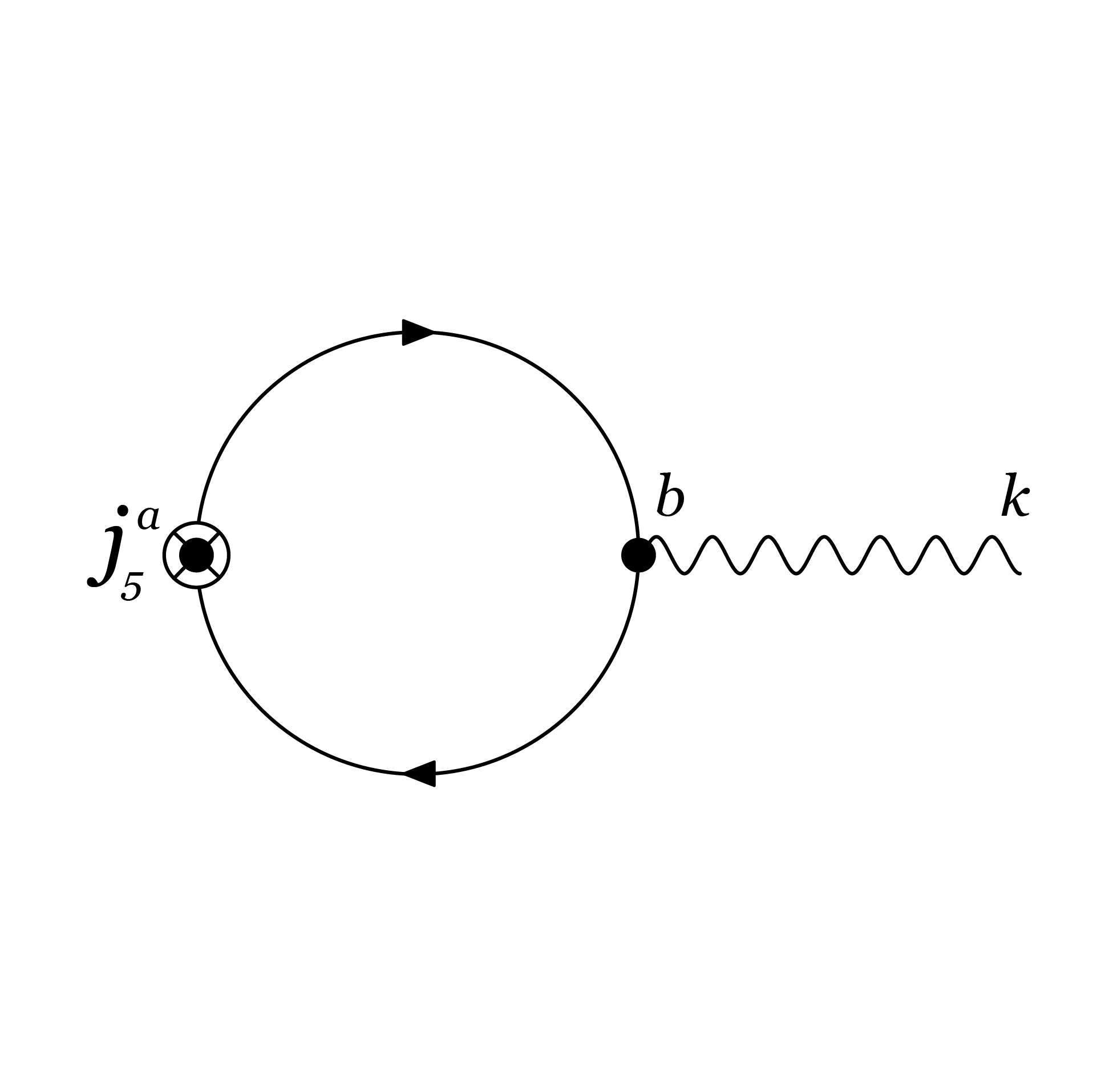
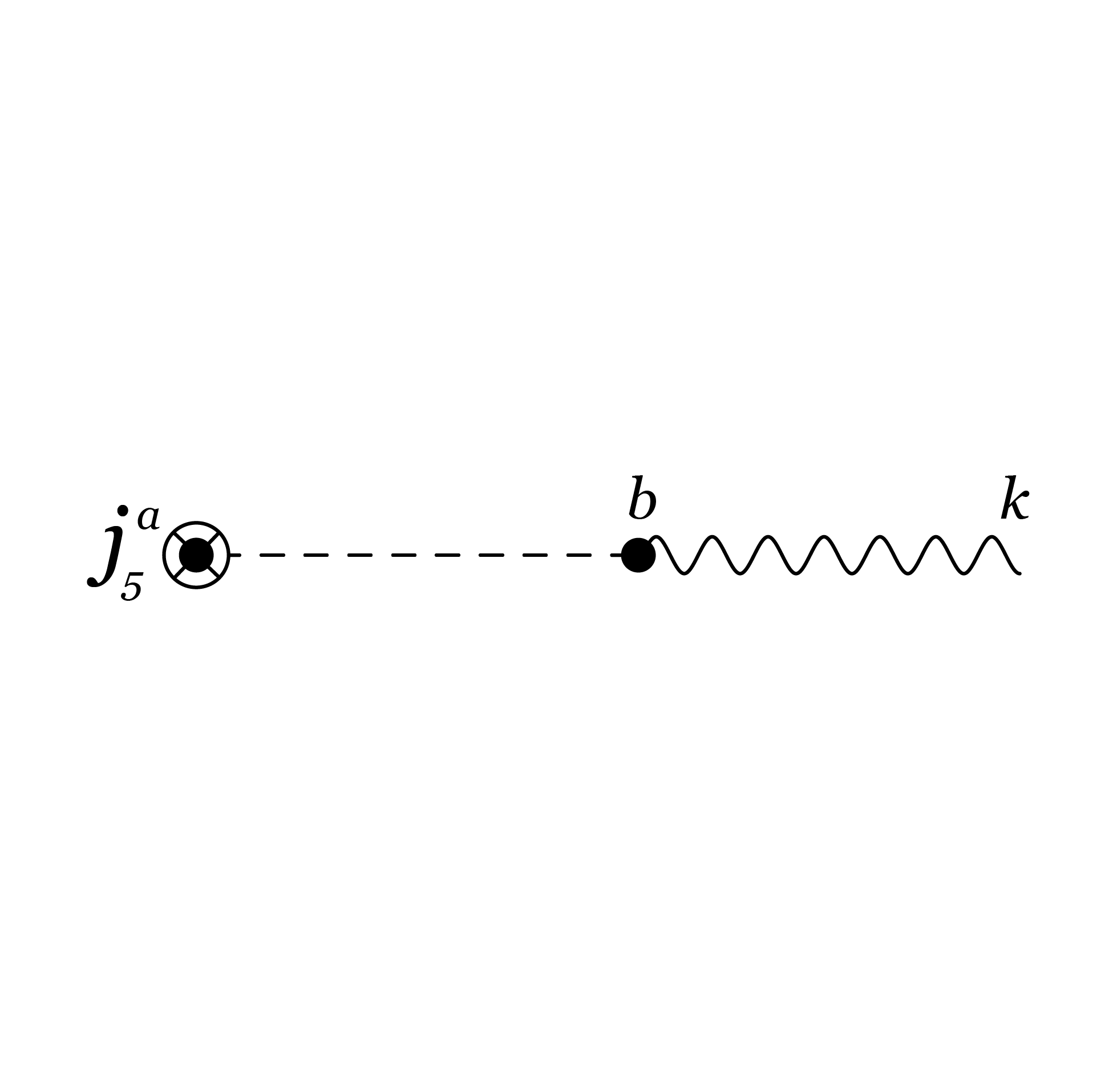
Figure 1: One-loop fermion polarization diagram (a) and equivalent pseudoscalar tree diagram (b).

The axial and vector currents may be expressed in terms of the effective boson $\chi$ field via

$$\tilde{j}^{a}=\partial^{a}\chi\,,\qquad\qquad j^{a}=\frac{\delta}{\delta A_{a}}\,S_{\rm eff}=-\epsilon^{ab}\partial_{b}\chi$$ (37)

so that the conservation of $j^{a}$ becomes a topological identity and the chiral anomaly (33) follows from the eq. of motion for $\chi$ (36). This is the chiral bosonization of fermion currents in $1+1$ dimensions Coleman (1975); Mandelstam (1975). The chiral boson $\chi$ obeys a massless wave eq. (36) with ${\mathscr{A}}_{2}$ as its source. It acquires a mass $M=e/\!\sqrt{\pi}$ only if the coupling $e\neq 0$ in the full Schwinger model of (28).

The explicit Fock space operator representation of the chiral boson in terms of fermion bilinears is given in Appendix B. These lead to the equal time commutator

$$\big{[}\chi(t,x),\dot{\chi}(t,x^{\prime})\big{]}=\frac{i}{\pi}\,\delta(x-x^{\prime})\vspace{-2mm}$$ (38)

which is exactly the canonical commutation relation obtained directly from the effective action (35). From (130)-(135) the fermion current densities in the Fock space representation are

$$j^{0} =\,\partial_{x}\chi\,=\,\tilde{j}^{1}$$ (39a)

$$j^{1} =\!-\partial_{t}\chi=\tilde{j}^{0}\vspace{-2mm}$$ (39b)

reproducing the bosonization relations (37) obtained in the effective action representation. These relations and the commutator (38) imply

$$\big{[}j^{0}(t,x),j^{1}(t,x^{\prime})\big{]}=-\frac{i}{\pi}\,\partial_{x}\,\delta(x-x^{\prime})$$ (40)

which is the Schwinger term in the equal time commutator of the current components Schwinger (1959); Jo (1985). The normal ordering prescription on the currents and precise definition of the fermion vacuum is essential to derive these commutation relations in the fermion representation.

Since the anomalous Schwinger current commutator in QED₂ is equivalent to the canonical commutator of the chiral boson $\chi$, it must be treated as a genuinely propagating collective degree of freedom, not apparent in the original fermionic action (28). Composed of fermion bilinears, analogous to Cooper pairs in condensed matter systems, $\chi$ has the massless propagator (32) which is associated with the axial anomaly Blaschke et al. (2014). The fermion bilinears are correlated/entangled fermion pairs in the two-fermion intermediate states of the polarization diagram Fig. 1, moving co-linearly at the speed $c=1$, and equivalent to a massless boson according to (130)-(134). Because of (37) the propagating wave solutions of (36) are jointly Chiral Density Waves and Charge Density Waves, arising from massless particle-hole excitations of the Dirac sea. As we shall now show, these same CDWs may also be regarded as acoustic modes in the superfluid hydrodynamic description at $T=0$, and thus the superfluid hydrodynamic description of Sec. II applies both to the filled Fermi-Dirac sea at non-zero chiral density, and the Dirac fermion vacuum itself.

III.2 Equivalence to Chiral Superfluid Hydrodynamics in $D=2$

At finite chiral chemical potential $\tilde{\mu}$, but $T\!=\!0$, massless fermions in $D\!=\!2$ have the energy density and pressure (cf. Appendix B)

$$\varepsilon=\frac{\pi}{2}\,\tilde{n}^{2}=p=\frac{1}{2\pi}\,\tilde{\mu}^{2}\qquad{\rm where}\qquad\tilde{\mu}=\pi\,\tilde{n}\,,\vspace{-2mm}$$ (41)

so that (5) gives at $\tilde{A}_{\lambda}=0$

$$\partial_{a}\eta=-\mbox{\small$\displaystyle\frac{\tilde{\mu}}{\tilde{n}}$}\ \tilde{j}_{a}=-\pi\,\tilde{j}_{a}=-\pi\,\partial_{a}\chi\vspace{-4mm}$$ (42)

since $\tilde{j}^{a}=\partial^{\alpha}\chi$ by the bosonization formulae (37).

The simple proportionality in (42) between the gradient of the $\eta$ potential and that of the a priori independent chiral boson field $\chi$ is what makes possible the identification of the Schwinger model with the chiral superfluid of Sec. II. Recalling (3) with (42) we now obtain

$$(\partial_{a}\eta)\,\tilde{j}^{a}-\varepsilon(\tilde{n})=-\pi\,(\partial_{a}\raisebox{0.7pt}{$\chi$})(\partial^{a}\raisebox{0.7pt}{$\chi$})+\frac{\pi}{2}\,\tilde{j}^{a}\,\tilde{j}_{a}=-\frac{\pi}{2}\,\big{(}\partial_{a}\chi\big{)}\big{(}\partial^{a}\chi\big{)}$$ (43)

for two of the terms in (1). Then integrating the relation (42), so that

$$\eta=-\pi\chi+\mbox{\small$\displaystyle\frac{\theta}{2}$}\vspace{-2mm}$$ (44)

where $\theta$ is a spacetime constant, and using (33) for the chiral anomaly ${{\mathscr{A}}}_{2}$ in $D\!=\!2$, we have

$$S_{\chi\rm sf}\Big{|}_{D=2,\,\tilde{A}^{a}=0}=\int\!\!d^{2}x\!\left\{-\frac{\pi}{2}\,\big{(}\partial_{a}\chi\big{)}\big{(}\partial^{a}\chi\big{)}-\chi\,^{*}\!F+\frac{\theta}{2\pi}\,^{*}\!F\right\}=S_{\rm eff}[\chi;A]+\frac{\theta}{2\pi}\int\!\!d^{2}x\!\ ^{*}\!F$$ (45)

Thus the hydrodynamic superfluid action (1), postulated on the basis only of macroscopic conservation laws for an irrotational and isentropic fluid with the axial anomaly is the microscopic QFT effective action of the zero temperature Schwinger model (35) up to a surface term, at zero coupling $e\!=\!0$. Note that the equivalence of the QFT to the chiral superfluid requires the addition of the (non-anomalous) $-\varepsilon(\tilde{n})$ energy density term in (43) to the effective action of the anomaly alone, for which the $\eta$ variation of the first two terms of (1) is sufficient to yield (4).

Since ${}^{*}\!F$ is a total divergence, addition of the constant $\theta$ term does not affect the local dynamics. Instead this term is related to the topology of the gauge field configuration space. This topology, periodicity in $\theta$ and hence $\eta$ or $\chi$ are made clear by careful treatment of the zero modes of the system in a finite linear spatial volume $L$ in the real time Hamiltonian formulation of Appendix C.

Since

$$[\eta(t,x),\Pi_{\eta}(t,x^{\prime})]=\pi\,[\raisebox{0.7pt}{$\chi$}(t,x),\dot{\raisebox{0.7pt}{$\chi$}}(t,x^{\prime})]=i\,\delta(x-x^{\prime})$$ (46)

the canonical commutation relation (20) of the superfluid hydrodynamic description coincides with the commutator (38) for the chiral boson of QED₂, which then implies the Schwinger term (40) in the current commutators. Since from (41) $\tilde{\mu}/\tilde{n}=\pi$ is a constant in $D\!=\!2$, the wave eq. of the hydrodynamic description (19) also coincides with that of the propagating chiral boson of $e=0$ electrodynamics (36) in two dimensions. Because of the simple relation (42), the CDW solutions for $\chi$ are also waves of the Clebsch potential $\eta$, which are the sound waves of the fluid. At finite equilibrium chiral density $\tilde{n}\neq 0$, these are CDW excitations of the Fermi surface at Fermi energy $\tilde{\mu}$. The vacuum limit $\tilde{\mu}\rightarrow 0,\tilde{n}\rightarrow 0$, with $\tilde{\mu}/\tilde{n}=\pi$ fixed shows that this description holds when the Fermi surface of filled positive energy single fermion states goes over to the Dirac fermion Fock vacuum where only the negative energy states of the Dirac sea are filled. In that limit the CDWs of the $\chi$ field become chiral waves on the Dirac vacuum sea itself.

IV Goldstone Theorem for Anomalous Symmetry Breaking

Since the axial anomaly with ${\mathscr{A}}_{D}\neq 0$ breaks chiral symmetry explicitly rather than spontaneously, it may seem at first sight that Goldstone’s theorem should not apply to ASB. However in the non-anomalous terms of the effective action (1) and Hamiltonian (17) the velocity potential $\eta$ appears only under derivatives, which therefore are left invariant by the constant shift symmetry $\eta\rightarrow\eta+\eta_{0}$. Moreover in the anomaly term $\eta$ multiplies ${\mathscr{A}}_{D}=\partial_{\lambda}K^{\lambda}$, a total derivative, with $K^{\lambda}$ the Chern-Simons current. Hence the total action (1) is also invariant under the constant phase shift transformation, up a topological term that does not affect the local dynamics. Thus we should expect a variant of Goldstone theorem in QFT to guarantee this gapless mode of the chiral superfluid described by (1) in a non-dynamical $A_{\lambda}$ gauge field background. In this section we show how Goldstone’s theorem can be extended to the new case of symmetry breaking by the axial anomaly (ASB), by use of the canonical commutator (20) of the superfluid Hamiltonian, which is equivalent to the Schwinger terms in the anomalous commutator of currents.

The main element needed for a proof of Goldstone’s theorem in the familiar case of SSB is the minimization of an effective potential at which some scalar order parameter assumes a non-zero expectation value $\langle\Phi\rangle\neq 0$ that is not invariant under the symmetry. In ASB, without assuming any effective potential to be minimized, the $\eta$ phase field does act as the natural order parameter of chiral symmetry breaking for the fermion theory. We shall now show that provided

$$\big{\langle}e^{2i\eta}\big{\rangle}=e^{2i\eta_{0}}\equiv z_{0}\neq 0$$ (47)

is both well-defined and non-vanishing in the ground state of the system, the necessary and sufficient condition for the existence of a massless Nambu-Goldstone boson Nambu and Jona-Lasinio (1961a, b); Goldstone et al. (1962) is satisfied.

That $\langle e^{2i\eta}\rangle$ plays the role of a complex phase order parameter characterizing chiral symmetry breaking is made clear by integrating (20) over the spatial volume. This gives

$$\big{[}\tilde{Q}(t),\eta(t,\boldsymbol{x})\big{]}=\int\!d^{d}\boldsymbol{x}^{\prime}\left[\tilde{J}^{0}(t,\boldsymbol{x}^{\prime}),\eta(t,\boldsymbol{x})\right]=-i$$ (48)

which is a c-number, whose further commutators with $\tilde{Q}$ vanish. Hence

$$e^{i\alpha\tilde{Q}(t)}\eta(t,\boldsymbol{x})e^{-i\alpha\tilde{Q}(t)} = \eta(t,\boldsymbol{x})+i\alpha\left[\tilde{Q}(t),\eta(t,\boldsymbol{x})\right]+\mbox{\small$\displaystyle\frac{(i\alpha)^{2}}{2}$}\Big{[}\tilde{Q}(t),\left[\tilde{Q}(t),\eta(t,\boldsymbol{x})\right]\Big{]}+\dots$$ (49)

$$= \eta(t,\boldsymbol{x})+\alpha\vspace{-4mm}$$

shifts $\eta(t,\boldsymbol{x})$ by a constant $\alpha$ under a global chiral rotation of magnitude $\alpha$. Therefore

$$e^{i\alpha\tilde{Q}(t)}e^{2i\eta(t,\boldsymbol{x})}e^{-i\alpha\tilde{Q}(t)}=\sum_{n=0}^{\infty}\mbox{\small$\displaystyle\frac{i^{n}}{n!}$}\,\big{(}2\eta(t,\boldsymbol{x})+2\alpha\big{)}^{n}=e^{2i\alpha}\,e^{2i\eta(t,\boldsymbol{x})}$$ (50)

as expected for a $2\pi$-periodic phase field associated with the breaking of global chiral symmetry.

IV.1 Lorentz Invariant Case

If in addition to (47) the vacuum is both Lorentz and translationally invariant, it follows that

$$\int d^{D}\!x\ e^{ik\cdot(x-y)}\,\big{\langle}{\cal T}^{*}\tilde{J}^{\lambda}(x)\,e^{2i\eta(y)}\big{\rangle}=ik^{\lambda}F(k^{2})$$ (51)

for some Lorentz invariant function $F(k^{2})$. Then we have

$$\frac{\partial}{\partial x^{\lambda}}\langle{\cal T}^{*}\tilde{J}^{\lambda}(x)\,e^{2i\eta(y)}\rangle=\delta(x^{0}-y^{0})\Big{\langle}\big{[}\tilde{J}^{0}(x),e^{2i\eta(y)}\big{]}\Big{\rangle}=2\,\delta^{D}(x-y)\,z_{0}$$ (52)

from the commutation relation (20), in the absence of gauge fields or limit of very weak coupling $e\!\to 0$ where the anomaly ${\mathscr{A}}_{D}=0$. Multiplying (51) by $-ik_{\lambda}\rightarrow-\partial/\partial x^{\lambda}$, integrating by parts and making use of (52) yields then

$$2z_{0}=k^{2}F(k^{2})\quad\Longrightarrow\quad F(k^{2})=\frac{2z_{0}}{\,k^{2}}\vspace{-2mm}$$ (53)

and therefore

$$\int d^{D}\!y\ e^{ik\cdot(x-y)}\,\big{\langle}{\cal T}^{*}\tilde{J}^{\lambda}(x)\,e^{2i\eta(y)}\big{\rangle}=2i\,\frac{k^{\lambda}}{k^{2}}\,\langle e^{2i\eta}\rangle$$ (54)

demonstrating the existence of the massless Nambu-Goldstone pole at $k^{2}=0$ in any $D\!=\!2n$ even dimension where (20) holds due to the axial anomaly Ward Identity, provided $z_{0}\neq 0$ in a Lorentz and translationally invariant state.

Thus the gapless acoustic mode of (19), derived from the Hamiltonian and commutation relations of the canonical pair $\{\eta,\Pi_{\eta}\}$, is indeed a consequence of Goldstone’s theorem, extended to this new case of ASB, symmetry breaking through the axial anomaly and anomalous Schwinger commutators. This establishes a microscopic QFT basis for superfluidity and a collective Goldstone sound mode in anomalous fermion systems.

We note that assuming the $\eta$ phase has a well-defined expectation value in (47) is a statement about long-range order in the ground state of the system, where $\eta$ is a composite or collective boson degree of freedom composed of fermion/anti-fermion pairs, as can be made explicit in $D\!=\!2$ by (44) and the fermion bosonization relations reviewed in Appendix B. Rather than the unmodified (non-anomalous) symmetry generators of SSB, we have employed the anomalous commutators required by the axial anomaly itself. The fact that (47) holds only approximately for a range of distance scales in $D\!=\!2$ where quasi-long-range order holds in the limit $e\!\to\!0$ but volume $L\!\to\!\infty$ is discussed in detail in Appendix C, where the relation to the fermion condensate and quasi-long-range-order is further explored. A gapless Goldstone mode related to the axial anomaly was discussed, in the context of universality of transport properties in chiral media in Alekseev et al. (1998).

IV.2 Goldstone Sound Mode in General Case of Anomalous Superfluid Hydrodynamics

The Goldstone mode propagates at the speed of light $c\!=\!1$ if and only if the ground state is Lorentz invariant as assumed in (47)-(52). This need not be the case. Indeed if the wave eq. (19) for the phase field $\eta$ in the superfluid description is linearized around its equilibrium solution

$$\eta = \tilde{\mu}\,t+\delta\eta$$ (55a)

$$\delta\left(\frac{\tilde{n}}{\tilde{\mu}}\right) = \frac{d}{\,d\tilde{\mu}}\left(\frac{\tilde{n}}{\tilde{\mu}}\right)\delta\tilde{\mu}=\frac{d}{\,d\tilde{\mu}}\left(\frac{\tilde{n}}{\tilde{\mu}}\right)\,\delta\dot{\eta}$$ (55b)

where $\delta\tilde{\mu}=\delta\dot{\eta}\,$ follows from variation of (8) and use of (55a) in the fluid rest frame. Then from the variation of (5) with $A_{5\lambda}=0$ we obtain

$$\delta\tilde{J}^{0} = \tilde{\mu}\,\delta\!\left(\frac{\tilde{n}}{\tilde{\mu}}\right)+\frac{\tilde{n}}{\tilde{\mu}}\,\delta\dot{\eta}=\left[\tilde{\mu}\frac{d}{d\tilde{\mu}\!}\!\left(\frac{\tilde{n}}{\tilde{\mu}}\right)+\frac{\tilde{n}}{\tilde{\mu}}\right]\delta\dot{\eta}=\frac{d\tilde{n}}{d\tilde{\mu}}\ \delta\dot{\eta}$$ (56a)

$$\delta\tilde{J}^{i} = -\frac{\tilde{n}}{\tilde{\mu}}\ \partial_{i}(\delta\eta)$$ (56b)

where the equilibrium (spacetime independent) values for $\tilde{n},\tilde{\mu}$ and their derivatives are to be used. Eqs. (56) can be combined and written in the covariant form

$$\delta\tilde{J}^{\lambda}=\frac{d\tilde{n}}{d\tilde{\mu}}\left[u^{\lambda}u^{\nu}\big{(}1-v_{s}^{2}\big{)}-v_{s}^{2}\,g^{\lambda\nu}\right]\partial_{\nu}(\delta\eta)$$ (57)

by use of the kinetic velocity $u^{\lambda}$ which is $\delta^{\lambda}_{\ 0}$ in the fluid rest frame, and

$$v_{s}^{2}\equiv\frac{\tilde{n}}{\tilde{\mu}}\frac{d\tilde{\mu}}{\,d\tilde{n}}=\frac{dp}{d\varepsilon}$$ (58)

by (6) and (10). Thus the wave eq. (19) linearized about equilibrium is

$$\partial_{\lambda}\big{(}\delta\tilde{J}^{\lambda}\big{)}=\frac{d\tilde{n}}{d\tilde{\mu}}\left(\frac{\partial^{2}}{\partial t^{2}}-v_{s}^{2}\,\nabla^{2}\right)\delta\eta=0$$ (59)

in the absence of the anomaly source, and the gapless Nambu-Goldstone mode propagates at speed $v_{s}\leq 1$, becoming the speed of light if and only if $\tilde{\mu}$ and $\tilde{n}$ are linearly related, and $p=\varepsilon$.

Upon quantization the relations (48)-(50) continue to hold for the variations $\delta J^{\lambda}$ and $\delta\eta$. Thus (51) may be reconsidered for the linearized variations away from the ground state of the general non-vanishing $\tilde{\mu},\tilde{n}$, and

$$\int\!dte^{-i\omega(t-t^{\prime})}\!\int d^{d}\!\boldsymbol{x}\ e^{i{\bm{k}}\cdot(\boldsymbol{x}-\boldsymbol{x}^{\prime})}\,\big{\langle}{\cal T}^{*}\delta\tilde{J}^{\lambda}(t,\boldsymbol{x})\,e^{2i\delta\eta(t^{\prime}\boldsymbol{x}^{\prime})}\big{\rangle}=-i\left[u^{\lambda}u^{\nu}\big{(}1-v_{s}^{2}\big{)}-v_{s}^{2}\,g^{\lambda\nu}\right]k_{\nu}F(\omega,|{\bm{k}}|)$$ (60)

in terms of a scalar function $F(\omega,|{\bm{k}}|)$, which follows from (57) and the fact that the variation of the velocity potential $\delta\eta$ and $\tilde{\mu},\tilde{n}$ are spacetime (pseudo)scalars. Repeating the steps leading to (53) leads then to

$$\left[-(k\cdot u)^{2}\big{(}1-v_{s}^{2}\big{)}+v_{s}^{2}\,k^{2}\right]F(\omega,|{\bm{k}}|)=\big{(}-\omega^{2}+v_{s}^{2}\,{\bm{k}}^{2}\big{)}F\big{(}\omega,|{\bm{k}}|\big{)}=2z_{0}$$ (61)

which implies

$$F\big{(}\omega,|{\bm{k}}|\big{)}=\frac{2z_{0}}{-\omega^{2}+v_{s}^{2}\,{\bm{k}}^{2}}$$ (62)

instead, showing the gapless acoustic propagator pole in superfluid hydrodynamics for general $v_{s}$.

An important point to notice about this derivation is that Lorentz invariance is spontaneously broken in general by a background $\tilde{\mu}$, and this is reflected in both the time dependence of (55a) and the necessity of taking the variation of the magnitude $\tilde{n}/\tilde{\mu}$ of the chiral current into account in (56a), this variation being responsible for the sound speed $v_{s}$ differing in general from the speed of light, although the acoustic CDW Goldstone mode remains gapless. It is also instructive to consider the variation of the energy-momentum tensor (22) linearized around a constant background $n_{5}$,

$$M^{\lambda\nu}\delta J_{5,\nu}\equiv\Bigg{\{}\left[g^{\lambda\nu}+u^{\lambda}u^{\nu}\left(1-v_{s}^{2}\right)\right]\left(u\cdot\partial\right)+u^{\lambda}\partial^{\nu}-v_{s}^{2}\,u^{\nu}\partial^{\lambda}\Bigg{\}}\delta J_{5,\nu}=0$$ (63)

which possesses non-trivial solutions in general $D\!=\!d+1$ dimensions only if the Fourier components of $\delta J_{5,\alpha}$ satisfy the relation

$$\det M=(-i\omega)^{d-1}\left[\omega^{2}-v_{s}^{2}|{\bm{k}}|^{2}\right]=0\,.\vspace{-2mm}$$ (64)

This is the same gapless condition as (62) for the Goldstone pole, showing that the only propagating mode in the non-dissipative anomalous superfluid is the gapless (first) sound mode.

V The Axial Anomaly and Effective Action in Four Dimensions

V.1 The Massless Pole in Four Dimensions

In $D\!=\!4$ dimensions the axial current $\tilde{J}^{\lambda}=J_{5}^{\lambda}=\bar{\psi}\gamma^{\lambda}\gamma_{5}\psi$ has the anomalous divergence

$$\partial_{\lambda}J^{\lambda}_{5}=e^{2}{\mathscr{A}}_{4}=\frac{\alpha}{2\pi}\,F^{\lambda\nu}\,{}^{*}\!F_{\lambda\nu}=\frac{2\alpha}{\pi}\,\boldsymbol{E\cdot B}$$ (65)

for massless fermions, where ${}^{*}\!F_{\lambda\nu}\equiv\frac{1}{2}\epsilon_{\lambda\nu\rho\sigma}F^{\rho\sigma}$ is the dual of the field strength tensor $F_{\lambda\nu}$ and $\alpha=e^{2}/4\pi$ Adler (1969); Adler and Bardeen (1969); Bell and Jackiw (1969); Treiman et al. (1972). The axial anomaly (65) in $D\!=\!4$ results from the one-loop triangle diagram of Fig. 2. In momentum space labeling $k=p+q$ the ingoing momentum at the axial vertex, and $p$ and $q$ the outgoing momenta on the photon legs, the triangle diagram may be evaluated explicitly

$$\Gamma^{\lambda\alpha\beta}(p,q)=\sum^{6}_{i=1}f_{i}(k^{2};p^{2},q^{2})\,\tau_{i}^{\lambda\alpha\beta}(p,q)$$ (66)

and expressed as a sum over six basis tensors $\tau_{i}^{\lambda\alpha\beta}(p,q)$ multiplied by scalar form factor functions $f_{i}$ of the three Lorentz invariants $k^{2},p^{2},q^{2}$. The coefficient functions $f_{i}$ are given e.g. in Refs. Rosenberg (1963); Giannotti and Mottola (2009) and for zero fermion mass are

$$f_{1}(k^{2};p^{2},q^{2})=f_{4}(k^{2};q^{2},p^{2})=\frac{4\alpha}{\pi}\int^{1}_{0}dx\int^{1-x}_{0}dy\frac{xy}{{\cal D}}$$ (67a)

$$f_{2}(k^{2};p^{2},q^{2})=f_{5}(k^{2};q^{2},p^{2})=\frac{4\alpha}{\pi}\int^{1}_{0}dx\int^{1-x}_{0}dy\frac{x(1-x)}{{\cal D}}$$ (67b)

$$f_{3}(k^{2};p^{2},q^{2})=f_{6}(k^{2};q^{2},p^{2})=0$$ (67c)

where the denominator ${\cal D}=(p^{2}x+q^{2}y)(1-x-y)+xyk^{2}$, in the basis where

$$\tau_{1}^{\lambda\alpha\beta}(p,q)=\tau_{4}^{\lambda\beta\alpha}(q,p)=-p\cdot q\,\epsilon^{\lambda\alpha\beta\gamma}p_{\gamma}-p^{\beta}\,\upsilon^{\lambda\alpha}(p,q)$$ (68a)

$$\tau_{2}^{\lambda\alpha\beta}(p,q)=\tau_{5}^{\lambda\beta\alpha}(q,p)=p^{2}\,\epsilon^{\lambda\alpha\beta\gamma}q_{\gamma}+p^{\alpha}\,\upsilon^{\lambda\beta}(p,q)$$ (68b)

and

$$\upsilon^{\alpha\beta}(p,q)\equiv\epsilon^{\alpha\beta\rho\sigma}\,p_{\rho}q_{\sigma}\,.$$ (69)

The two tensors $\tau_{3},\tau_{6}$ are linearly dependent on the other four and redundant, and in any case unnecessary because of (67c). The Feynman parameter integrals for $f_{i}$ in (67) can be evaluated in terms of digamma functions Armillis et al. (2009), but these explicit expressions will not be needed in the following.

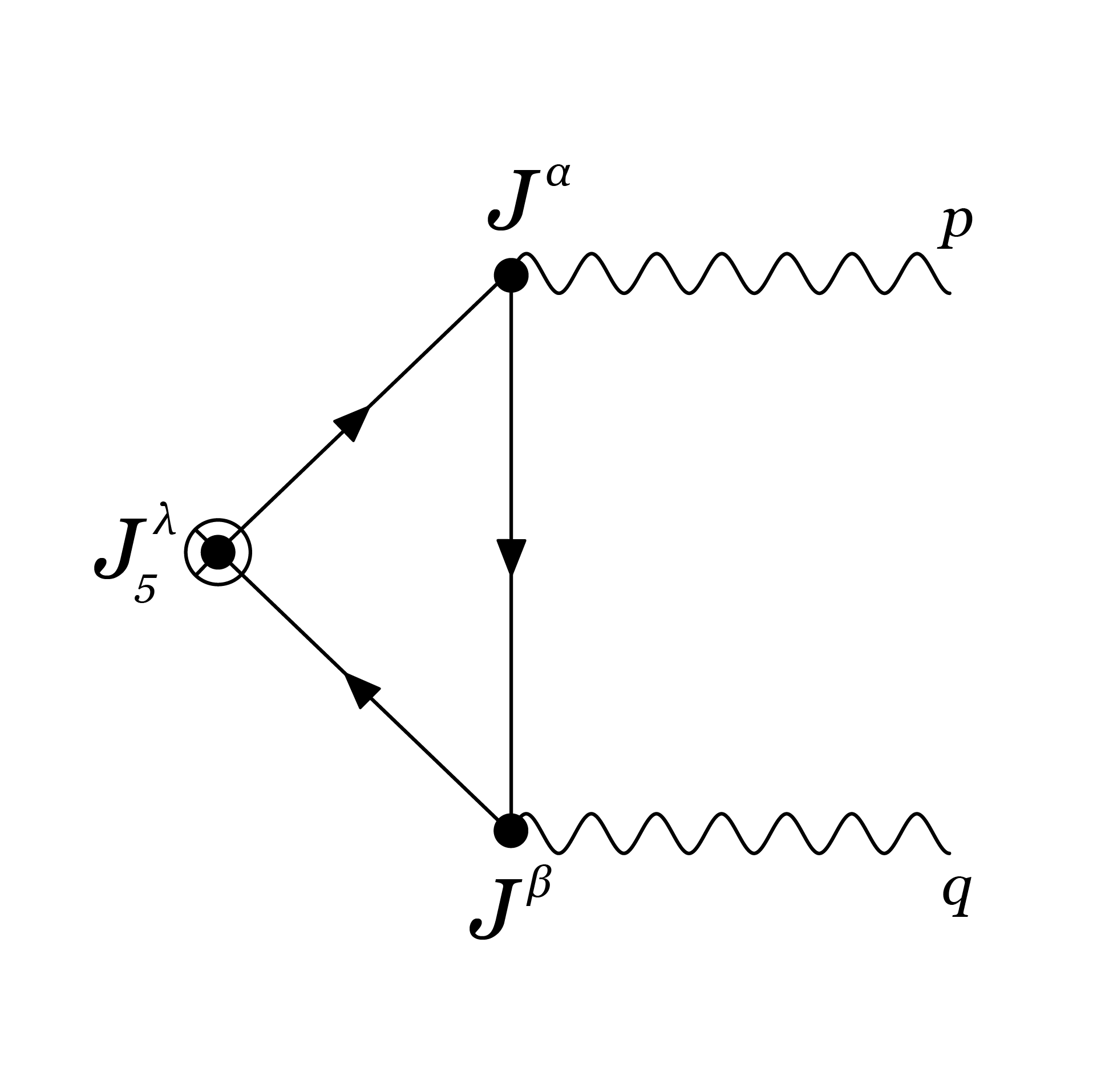
Figure 2: The Axial Anomaly Triangle Diagram Amplitude $\Gamma^{\lambda\alpha\beta}(p,q)$

If the current $J^{\lambda}_{5}$ is decomposed into its longitudinal and transverse components

$$J^{\lambda}_{5}=J^{\lambda}_{5\,\parallel}+J^{\lambda}_{5\perp}\,,\qquad\qquad\partial_{\lambda}J^{\lambda}_{5\perp}=0$$ (70)

it is clear that only the longitudinal component $J^{\lambda}_{5\,\parallel}$ contributes to the anomalous divergence (65). Similarly the triangle amplitude (66) may be decomposed into its longitudinal and transverse parts

$$\Gamma^{\lambda\alpha\beta}(p,q)=\Gamma^{\lambda\alpha\beta}_{\parallel}(p,q)+\Gamma_{\perp}^{\lambda\alpha\beta}(p,q)\,,\qquad\qquad k_{\lambda}\,\Gamma_{\perp}^{\lambda\alpha\beta}(p,q)=0$$ (71)

so that the transverse part does not contribute to the anomaly. The longitudinal part explicitly exhibits a $1/k^{2}$ pole, and gives the total anomaly

$$\Gamma^{\lambda\alpha\beta}_{\parallel}(p,q)=\frac{2\alpha}{\pi}\,\frac{k^{\lambda}}{k^{2}}\,\upsilon^{\alpha\beta}(p,q)\,,\qquad\qquad k_{\lambda}\Gamma^{\lambda\alpha\beta}(p,q)=k_{\lambda}\Gamma^{\lambda\alpha\beta}_{\parallel}(p,q)=\frac{2\alpha}{\pi}\,\upsilon^{\alpha\beta}(p,q)$$ (72)

which is (65) in momentum space. As in $D\!=\!2$ the appearance of the $1/k^{2}$ pole in (71) signals that the anomaly is associated with a massless pseudoscalar collective excitation, here and in higher dimensions residing in the longitudinal subsector of the full theory. Whereas the form of the axial anomaly and hence the longitudinal sector of the axial current with its $1/k^{2}$ pole is protected at higher loop orders by the Adler-Bardeen theorem Adler and Bardeen (1969), the transverse sector is not so protected.

Since the longitudinal projection of $J^{\lambda}_{5}$ is

$$J^{\lambda}_{5\,\parallel}=\partial^{\lambda}\left(\,\raise 0.5pt\hbox{$\vbox{\hrule\hbox{\vrule height=7.22743pt\kern 7.22743pt\vrule} \hrule}$}\,^{-1}\partial_{\nu}J^{\nu}_{5}\right)\vspace{-2mm}$$ (73)

the axial anomaly (65) corresponds to the non-local one-loop 1PI quantum effective action Giannotti and Mottola (2009); Blaschke et al. (2014)

$$S_{\rm anom}^{NL}[A,A_{5}]\!=\!\frac{\alpha}{2\pi}\!\int\!d^{4}x\!\int\!d^{4}y\,[A^{5}_{\mu}\,\partial^{\mu}]_{x}\,\raise 0.5pt\hbox{$\vbox{\hrule\hbox{\vrule height=7.22743pt\kern 7.22743pt\vrule} \hrule}$}\,^{-1}_{xy}\,[F^{\lambda\nu}\,{}^{*}\!F_{\lambda\nu}]_{y}$$ (74)

where $\,\raise 0.5pt\hbox{$\vbox{\hrule\hbox{\vrule height=7.22743pt\kern 7.22743pt\vrule} \hrule}$}\,^{-1}_{xy}=\frac{1\,}{4\pi^{2}}\,(x-y)^{-2}$ denotes the massless scalar propagator in $D\!=\!4$. The appearance of the massless $1/k^{2}$ pole (71) and massless scalar propagator $\,\raise 0.5pt\hbox{$\vbox{\hrule\hbox{\vrule height=7.22743pt\kern 7.22743pt\vrule} \hrule}$}\,^{-1}_{xy}$ in (74), in the longitudinal sector of the $D\!=\!4$ axial anomaly is thus a simple kinematic consequence of the anomalous Ward Identity for the axial current. As in $D\!=\!2$ it leads to the expectation that it is related to anomalous chiral symmetry breaking and Goldstone’s theorem of Sec. IV, although the $\eta$ phase field has not yet been identified, and will appear only in the local form of anomaly effective action of (75) below.

V.2 Local Effective Action and Anomalous Current Commutators in $D\!=\!4$

As in the $D\!=\!2$ case, the massless boson degree of freedom represented by the $1/k^{2}$ pole in (71) or $\,\raise 0.5pt\hbox{$\vbox{\hrule\hbox{\vrule height=7.22743pt\kern 7.22743pt\vrule} \hrule}$}\,^{-1}_{xy}$ in (74) is a collective mode of a fermion pair intermediate state in the anomaly amplitude Giannotti and Mottola (2009). That it is also a CDW may be made explicit by expressing the non-local action (74) in a local bosonic form. Since the non-local action (74) involves the axial potential $A^{5}_{\lambda}$ and $[F\,^{*}\!F]$ asymmetrically, expressing this action in a local form apparently requires the introduction of two pseudoscalar fields ($\eta,\chi$), as suggested in Giannotti and Mottola (2009). Unlike in $D\!=\!2$, (75) is only part of the 1PI effective action of QED₄, with the dependence upon the transverse component $J_{5\perp}^{\lambda}$ not fixed by the anomaly. If two fields ($\eta,\chi$) are varied independently, a second massless wave eq. would result, apparently implying the existence of two independent gapless modes. However this is not warranted by the triangle amplitude (66) itself where only a single $1/k^{2}$ pole appears.

The previous $D\!=\!2$ example and chiral fluid action provides the way around this problem. Thus rather than introducing two scalar fields, consider instead the local anomaly action

$$S_{\rm anom}[\eta;A,A_{5}]=\!\!\int\!\!d^{4}x\!\left\{\big{(}\partial_{\lambda}\eta+A^{5}_{\lambda}\big{)}\,J_{5}^{\lambda}+\eta{\mathscr{A}}_{4}\right\}$$ (75)

together with the variational principle that this effective action should be stationary against variations of the axial current $J_{5}^{\lambda}$. Then $J_{5}^{\lambda}$ acts as a Lagrange multiplier field enforcing the constraint, $\partial_{\lambda}\eta+A^{5}_{\lambda}=0$, in the absence of any $\varepsilon$ term added to (75). Solving this constraint for $\eta$

$$\eta=-\,\raise 0.5pt\hbox{$\vbox{\hrule\hbox{\vrule height=7.22743pt\kern 7.22743pt\vrule} \hrule}$}\,^{-1}\partial^{\lambda}A_{\lambda}^{5}=-\,\raise 0.5pt\hbox{$\vbox{\hrule\hbox{\vrule height=7.22743pt\kern 7.22743pt\vrule} \hrule}$}\,^{-1}\partial^{\lambda}A_{\lambda\,\parallel}^{5}$$ (76)

and substituting this back into (75) reproduces exactly the required non-local action (74) with its massless pole. Variation of $S_{\rm anom}$ with respect to $\eta$ also reproduces the axial anomaly (65). The local action (75) does not require the introduction of a second scalar field, and this variational principle of $\delta S_{\rm anom}/\delta J_{5}^{\lambda}=0$ does not lead to a second independent massless mode, but (75) together with the variational principle for the axial current is completely equivalent to the effective action (74) derived directly from the fermionic QFT axial anomaly.

That a single bosonic degree of freedom is described by (75) is made clear by defining the momentum canonically conjugate to $\eta$

$$\Pi_{\eta}=\frac{\delta}{\delta\dot{\eta}}S_{\rm anom}=J_{5}^{0}\vspace{-2mm}$$ (77)

as in (11), which then implies the equal time commutator

$$\big{[}\eta(t,\boldsymbol{x}),\Pi_{\eta}(t,\boldsymbol{x}^{\prime})\big{]}=\big{[}\eta(t,\boldsymbol{x}),J^{0}_{5}(t,\boldsymbol{x}^{\prime})\big{]}=i\,\delta^{3}(\boldsymbol{x}-\boldsymbol{x}^{\prime})$$ (78)

upon quantization. Thus $\eta$ and $J^{0}_{5}$ form a single canonical pair, and hence describe just a single gapless bosonic degree of freedom associated with the $U^{ch}(1)$ chiral anomaly in $D\!=\!4$, as in $D\!=\!2$.

Furthermore the electromagnetic current due to the axial anomaly may be found from

$$J^{\lambda}=\frac{\delta S_{\rm anom}}{\delta A_{\lambda}\ }=\frac{\alpha}{2\pi}\frac{\delta}{\delta A_{\lambda}}\int\!\!d^{4}x\,\eta\,F^{\mu\nu}\,{}^{*}\!F_{\mu\nu}=\frac{2\alpha}{\pi}\,\,^{*}\!F^{\lambda\nu}\,\partial_{\nu}\eta$$ (79)

in terms of $\eta$, which has the components

$$J^{0}=-\frac{2\alpha}{\pi}\,{\boldsymbol{B}\cdot\nabla}\eta$$ (80a)

$${\boldsymbol{J}}=\frac{2\alpha}{\pi}\big{(}{\boldsymbol{B}}\,\dot{\eta}-{\boldsymbol{E}\times\nabla}\eta\big{)}\,.\vspace{-2mm}$$ (80b)

Then making use of (78), we have

$$\big{[}J^{0}(t,\boldsymbol{x}),J^{0}_{5}(t,\boldsymbol{x}^{\prime})\big{]} = -\frac{2i\alpha}{\pi}\,{\boldsymbol{B}\cdot\nabla_{\boldsymbol{x}}}\,\delta^{3}(\boldsymbol{x}-\boldsymbol{x}^{\prime})$$ (81a)

$$\big{[}{\boldsymbol{J}}(t,\boldsymbol{x}),J^{0}_{5}(t,\boldsymbol{x}^{\prime})\big{]} = -\frac{2i\alpha}{\pi}\,{\boldsymbol{E}\times\nabla_{\boldsymbol{x}}}\,\delta^{3}(\boldsymbol{x}-\boldsymbol{x}^{\prime})\hskip 14.22636pt$$ (81b)

in a background electric or magnetic field Adler and Boulware (1969); Gross and Jackiw (1969); Treiman et al. (1972). Like the axial anomaly (65) itself, these current commutator Schwinger terms are anomalous, in the sense that they are apparently zero if the unregularized Dirac fermion anti-commutation relations are used. As in $D\!\!=2$ these Schwinger commutator terms in fermionic currents are in fact a consequence of the axial anomaly, and follow necessarily from the canonical commutator (20) of the bosonic effective action of the axial anomaly (75), which therefore passes an important consistency check, showing that there is a single bona fide pseudoscalar collective degree of freedom which is not apparent at the classical level or the free Dirac theory, that is necessarily associated with the $U^{ch}(1)$ chiral anomaly also in $D\!=\!4$.

Let us emphasize that the Schwinger terms (81) in the current commutators depend only upon the longitudinal anomalous part of the triangle diagram, represented by (75). Other commutators and in particular $\big{[}J^{0}(t,\boldsymbol{x}),{\boldsymbol{J}}_{5}(t,\boldsymbol{x}^{\prime})\big{]}$ which depend upon the transverse part of the amplitude $\Gamma_{\perp}^{\lambda\alpha\beta}(p,q)$ are not determined by $S_{\rm anom}$, not protected by the Adler-Bardeen theorem Adler and Bardeen (1969), and can be canceled by regularization scheme dependent ‘seagull’ terms, hence removed entirely Adler and Boulware (1969); Treiman et al. (1972). The essential and unavoidable anomalous current commutators are (81), and these are entirely accounted for the local anomalous effective action (75), together with the canonical commutation relation (78) it implies for a single bona fide bosonic degree of freedom.

V.3 Chiral Magnetic and Separation Effects from the Anomaly Effective Action

The axial anomaly effective action (75) succinctly incorporates several macroscopic chiral effects. Making use of (80b) in the case of a constant uniform $\boldsymbol{B}$ field, we find

$${\boldsymbol{J}}=\frac{2\alpha}{\pi}\,\mu_{5}\,\boldsymbol{B}$$ (82)

in the Lorentz frame where $\boldsymbol{\nabla}\eta=0$, and $\dot{\eta}=\mu_{5}$ (changing notation $\tilde{\mu}=\mu_{5}$ in $D\!=\!4$). This is the Chiral Magnetic Effect (CME), which has been discussed in the literature in various contexts Vilenkin (1980); Kharzeev et al. (2008); Fukushima et al. (2008); Buividovich et al. (2009); Kharzeev and Warringa (2009); Son and Surowka (2009); Pu et al. (2011); Sadofyev and Isachenkov (2011); Sadofyev et al. (2011); Kalaydzhyan and Kirsch (2011); Hoyos et al. (2011); Nair et al. (2012); Son and Yamamoto (2012); Stephanov and Yin (2012); Jensen (2012); Fukushima (2013); Khaidukov et al. (2018); Avdoshkin et al. (2016).

Since the longitudinal projection of the chiral current can be expressed as the pure gradient (73), one can define $\chi\equiv\,\raise 0.5pt\hbox{$\vbox{\hrule\hbox{\vrule height=7.22743pt\kern 7.22743pt\vrule} \hrule}$}\,^{-1}\partial_{\nu}J^{\nu}_{5}$, and express the axial anomaly in the form

$$\partial_{\lambda}J^{\lambda}_{5}=\partial_{\lambda}J^{\lambda}_{5\parallel}=\,\raise 0.5pt\hbox{$\vbox{\hrule\hbox{\vrule height=7.22743pt\kern 7.22743pt\vrule} \hrule}$}\,\chi={\mathscr{A}}_{4}=\frac{2\alpha}{\pi}\,{\boldsymbol{E}\cdot\boldsymbol{B}}$$ (83)

of a massless wave eq. for the local $\chi$ field describing the gapless bosonic mode, with the chiral anomaly as its source, just as in the $D\!=\!2$ case (36). Analogously to $D\!=\!2$ this gapless mode is a collective mode of the two-fermion intermediate state in the anomaly amplitude, if fermion masses and interactions can be neglected, and is a CDW in $J^{\lambda}_{5}$. The components of the axial current expressed in terms of $\chi$ are

$$J^{0}_{5}=J^{0}_{5\parallel}=-\dot{\chi}$$ (84a)

$${\boldsymbol{J}}_{5}={\boldsymbol{J}}_{5\parallel}={\bf\nabla}\chi\,.\vspace{-2mm}$$ (84b)

In a static, constant ${\boldsymbol{B}}=B\bf\hat{x}$ field and parallel static electric field ${\boldsymbol{E}}=-\nabla\Phi=-{\bf\hat{x}}\,\frac{d\Phi}{dx}$ in the same direction, (83) becomes

$$\frac{d}{dx}\left(\frac{d\chi}{dx}\right)=-\frac{2\alpha}{\pi}\frac{d\Phi}{dx}\,B$$ (85)

assuming also $\chi=\chi(x)$. Integrating this once and substituting into (84b) gives

$${\boldsymbol{J}}_{5}=\nabla\raisebox{0.7pt}{$\chi$}=\frac{2\alpha}{\pi}\,\mu\,\boldsymbol{B}$$ (86)

upon taking $\Phi=-\mu$ for the charge chemical potential. In this way the Chiral Separation Effect (CSE) is also implied by and follows simply and directly from the axial anomaly.

V.4 Anomalous Hall Effect

Yet another macroscopic effect which is succinctly captured by the anomalous effective action (75) is the Anomalous Hall Effect (AHE) in a Weyl semi-metal. A good model for a Weyl semi-metal is given by the Dirac theory with an external constant axial field $\boldsymbol{A}_{5}=\Delta\boldsymbol{k}$, with only spatial components corresponding to a shift $\Delta\boldsymbol{k}$ between the Weyl nodes in momentum space Zyuzin and Burkov (2012); Hosur and Qi (2013); Goswami and Tewari (2013). In other words the fermionic spectrum is linear in momentum but the energies of right- and left-handed fermions reach zero at different points separated by $\boldsymbol{A}_{5}$. In the presence of a constant $\boldsymbol{A}_{5}$ and a background electric field the current (80b) obtained by varying the anomaly effective action is

$${\boldsymbol{J}}=-\frac{2\alpha}{\pi}{\boldsymbol{E}\times\nabla}\eta=-\frac{2\alpha}{\pi}\,\boldsymbol{A}_{5}\times\boldsymbol{E}\vspace{-2mm}$$ (87)

where we use that $\boldsymbol{\nabla}\eta=-\boldsymbol{A}_{5}$ corresponds to a constant axial field (75). This implies a linear phase shift in the chiral field $\eta=-\Delta\boldsymbol{k}\cdot\boldsymbol{x}$ in the effective action responsible for the AHE Zyuzin and Burkov (2012); Hosur and Qi (2013); Goswami and Tewari (2013); Kim et al. (2014).

Thus the macroscopic CME, CSE, and AHE are all consequences of the same effective action (75), which is derived directly from and equivalent to the bosonic form of the microscopic fermion QFT of the axial triangle anomaly (74) with its massless pole, on the one hand, and identical to the corresponding terms in the general chiral superfluid effective action (1) on the other.

VI Dimensional Reduction and Chiral Magnetic Waves

Unlike the case in $D\!=\!2$, the vacuum triangle amplitude (66) in massless QED₄ has both longitudinal and transverse parts. Since the anomaly action (75) takes account only of the longitudinal projection of the anomalous triangle diagram of massless fermions in QED₄, and provides no information about the transverse part of the chiral current, it is clearly incomplete. The action (75) is also incomplete in that it contains no $J^{\lambda}_{5}$ dependence other than the minimal linear $(\partial_{\lambda}\eta+A^{5}_{\lambda})\,J_{5}^{\lambda}$ term, which results in the simple constraint $\partial_{\lambda}\eta=-A_{\lambda}^{5}$, and hence no relation between the $\eta$ potential and the chiral current, analogous to (42) in $D\!=\!2$. It is that relation that enabled us to identify the propagating massless chiral boson $\chi$ of the bosonized Schwinger model, satisfying (36) with the Goldstone boson of the chiral superfluid description in (19). This relation and the identity of the fluid action with that of the Schwinger model resulted from adding the non-anomalous energy density $-\varepsilon(\tilde{n})$ of (41) to the effective action of the anomaly.

In this section, we show that in the special case of a constant, uniform magnetic field background the transverse part of the anomaly amplitude (66) vanishes, and the four dimensional axial anomaly reverts to the $D\!=\!2$ case, and moreover with a simple completion of $-\varepsilon(\tilde{n})$, the CDW of dimensional reduction coincides with a Chiral Magnetic Wave (CMW) along the magnetic field direction.

Let $\boldsymbol{B}\!=\!F_{23}(0)\,\bf\hat{x}$ have only a zero momentum component in the $\bf\hat{x}$ direction with $A_{\beta=2,3}(q)$ the corresponding gauge potential in the transverse $\bf\hat{y}$, $\!\bf\hat{z}$ directions as $q\!\rightarrow\!0$. Computing $\Gamma^{\lambda\alpha\beta}(p,q)A_{\beta}(q)$ in this limit, only the tensors $\tau_{1}$ and $\tau_{2}$ in (66) which are linear in $q$ contribute (as they are necessary to form a gauge invariant magnetic field source), but we can neglect $q$ and $q^{2}$ otherwise, setting $k=p+q\rightarrow p$ and $k^{2}=p^{2}$ in the denominator ${\cal D}$ of (67). Thus ${\cal D}=k^{2}x(1-x)$ in this limit, and the Feynman parameter integrals (67) are trivially evaluated to give

$$f_{2}=2f_{1}=\frac{2\alpha}{\pi k^{2}}\qquad{\rm for}\qquad q^{2}=0\,.$$ (88)

Then taking ${\boldsymbol{k}}_{\perp}\!=\!{\boldsymbol{p}}_{\perp}\!=\!0$ in the transverse $\bf\hat{y}$, $\bf\hat{z}$ directions and noting that $k_{\nu}F^{\nu\lambda}(q)=0$, we find

$$\lim_{q\rightarrow 0}\Gamma^{\lambda\alpha\beta}(k-q,q)A_{\beta}(q)\Big{|}_{\boldsymbol{k}_{\perp}=0} = \frac{2i\alpha}{\pi k^{2}}\left(k^{2}\delta^{\alpha}_{\ \nu}-k^{\alpha}k_{\nu}\right)\tilde{F}^{\lambda\nu}$$ (91)

$$= \left\{\begin{array}[]{cc}2i\alpha B\,\Pi_{2}^{ac}(k)\epsilon^{\ b}_{c}&{\rm if}\qquad\alpha=a,\ \lambda=b\\ 0&{\rm otherwise}\end{array}\right.$$

where $\alpha=a\,,\lambda=b$ range only over the $0,1$ subspace of the $D\!=\!4$ spacetime and $\Pi_{2}^{ab}(k)$ is the $D\!=\!2$ vacuum polarization of (31). Thus, the full triangle diagram contracted with a constant uniform magnetic field reduces to the 2D anomalous self-energy polarization of Fig. 1, and the $1/k^{2}$ pole in the 4D triangle anomaly becomes at ${\bf k}_{\perp}=0$ precisely the $1/k^{2}$ propagator pole of the effective boson $\chi$ in the 2D two-point polarization tensor $\langle j^{a}j^{c}_{5}\rangle$ of (30).

As a consistency check we may calculate the longitudinal part of the triangle amplitude (72) directly. Contracting $\Gamma_{\parallel}^{\lambda\alpha\beta}(p,q)$ with $A^{\beta}(q)$ and taking the same kinematic limit as in (91) we find

$$\lim_{q\rightarrow 0}\Gamma^{\lambda\alpha\beta}_{\parallel}(k-q,q)A_{\beta}(q)\Big{|}_{{\boldsymbol{k}}_{\perp}={\boldsymbol{p}}_{\perp}=0}=\lim_{q\rightarrow 0}\frac{2\alpha}{\pi}\frac{k^{\lambda}}{k^{2}}v^{\alpha\beta}(p,q)A_{\beta}(q)=-2i\,\frac{\alpha}{\pi}\,\frac{k^{\lambda}}{k^{2}}\,\tilde{F}^{\alpha\rho}k_{\rho}$$ (92)

where the only surviving indices are two-dimensional ranging over $t,x$. Then $\tilde{F}^{ab}=\epsilon^{ab}B$ for the 2D subspace of 4D spacetime and the Schouten relation for $\epsilon^{ab}$ (cf. Appendix A) results in

$$\lim_{q\rightarrow 0}\Gamma^{ca\beta}_{\parallel}(p,q)A_{\beta}(q)\Big{|}_{{\boldsymbol{k}}_{\perp}={\boldsymbol{p}}_{\perp}=0}=\ \frac{2i\alpha B}{\pi k^{2}}\left(k^{2}\delta^{a}_{\ b}-k^{a}k_{b}\right)\epsilon^{cb}$$ (93)

which coincides with (91). This proves that the transverse part of the anomalous triangle diagram does not contribute in the dimensional reduction limit of a constant, uniform magnetic field, which is accounted for completely by its longitudinal part and $1/k^{2}$ pole, which in this limit of ${\bm{k}}_{\perp}=0$ becomes precisely the $1/k^{2}$ pole of the $D\!=\!2$ Schwinger model of Sec. III.1.

A third, and independent non-perturbative check of dimensional reduction is to make use of the polarization operator of fermions in a constant, uniform magnetic field in the Lowest Landau Level (LLL) approximation

$$\big{\langle}{\cal T}^{*}J^{a}(t,x,{\bf y})J^{b}_{5}(t,x^{\prime},{\bf y}^{\prime})\big{\rangle}_{{}_{\!\!LLL}}=2\alpha B\!\int\!\frac{d\omega}{2\pi}\!\int\!\frac{dk}{2\pi}\!\int\!\frac{d^{2}{\bf k}_{\perp}}{(2\pi)^{2}}\,e^{ik(x-x^{\prime})+i{\bf k}_{\perp}\cdot({\bf y}-{\bf y}^{\prime})}\exp\!\left(\!-\frac{k_{\perp}^{2}}{2eB}\right)\Pi_{2}^{ac}(\omega,k)\epsilon_{c}^{\ b}$$ (94)

given in terms of the $D\!=\!2$ polarization (31) with $a,b=t,x$ Loskutov and Skobelev (1976); Calucci and Ragazzon (1994); Gusynin et al. (1995, 1999); Fukushima (2011); Miransky and Shovkovy (2015). The exponential dependence of this expression upon $1/eB$ is obtained by treating the magnetic field background exactly, rather than in first order perturbation theory of (66). Nevertheless, when we integrate (94) over the transverse ${\bf y}$, thereby setting ${\bf k}_{\perp}\!=\!0$, and evaluate the current commutator expectation

$$\Big{\langle}\big{[}J^{0}(t,x,{\bf y}),J^{0}_{5}(t,x^{\prime},{\bf y}^{\prime})\big{]}\Big{\rangle}_{{}_{\!\!LLL}}=\!\int\!\frac{d\omega}{2\pi}\!\int\!\frac{dk}{2\pi}\!\int\!\frac{d^{2}{\bf k}_{\perp}}{(2\pi)^{2}}\,e^{ik(x-x^{\prime})+i{\bf k}_{\perp}\cdot({\bf y}-{\bf y}^{\prime})}\big{\{}2\,{\rm Im}\,\Pi_{2}^{01}(\omega+i\epsilon,k)\big{\}}$$ (95)

from the imaginary part of (94), we find

$$\int d^{2}{\bf y}\Big{\langle}\big{[}J^{0}(t,x,{\bf y}),J^{0}_{5}(t,x^{\prime},{\bf y}^{\prime})\big{]}\Big{\rangle}_{{}_{\!\!LLL}}=2\alpha B\!\int\!\frac{d\omega}{2\pi}\!\int\!\frac{dk}{2\pi}\,e^{ik(x-x^{\prime})}\left\{2\,{\rm Im}\,\Pi_{2}^{01}(\omega+i\epsilon,k)\right\}$$

$$\hskip 36.98866pt=2\alpha B\,\Big{\langle}\big{[}j^{0}(t,x),j^{1}(t,x^{\prime})\big{]}\Big{\rangle}=-\frac{2i\alpha B}{\pi}\,\frac{\partial}{\partial x}\,\delta(x-x^{\prime})$$ (96)

consistent with the anomalous commutators (81a) derived from the $D\!=\!4$ triangle amplitude, simply proportional to the $D\!=\!2$ current commutator (40).

The fact that the LLL approximation saturates the anomalous commutator is consistent with the fact that only the LLL in a constant magnetic field has gapless excitations, so that if an external electric field is turned on adiabatically only fermions in the LLL can be excited, and the $D\!=4\!$ axial anomaly factorizes into its $D\!=\!2$ counterpart with a transverse density proportional to the magnetic field strength $B$ Nielsen and Ninomiya (1983); Basar and Dunne (2013).

Lastly, it is clear that in a constant uniform magnetic field with $\boldsymbol{E}(t,x)$ along the $\boldsymbol{B}$ direction, the four dimensional axial anomaly (65) becomes a simple factor $2\alpha B$ times the two dimensional axial anomaly (33). In this case the four dimensional ${\mathds{R}}^{4}$ base manifold factorizes into ${\mathds{R}}^{2}\!\otimes\!{\mathds{R}}^{2}$, and the topology of the gauge field mapping the periodic $x$ domain to the gauge field configuration space ${\mathds{S}}^{1}\rightarrow{\mathds{S}}^{1}$ applies just as in Appendix C, as does the Atiyah-Singer index theorem in $D\!=\!2$ Rupertsberger (1981). Thus we should expect all aspects of the previous $D\!=\!2$ analysis of superfluid CDW and Schwinger boson to carry over directly to $D\!=\!4$ in a constant uniform magnetic field background with simple replacement of the $D\!=\!2$ dimensional coupling $e^{2}$ by $2\alpha B$ in $D\!=\!4$ That this CDW Schwinger boson following directly from the anomaly effective action (75) is in fact the Chiral Magnetic Wave (CMW) discussed in the literature by several authors Kharzeev and Yee (2011) may be seen as follows.

If in addition to the constant uniform magnetic field $B$ the massless fermions in the LLL are placed in a state of small but non-zero chiral chemical potential $\mu_{5}^{2}\ll eB$, the relation between $n_{5}$ and $\mu_{5}$ is linear, cf. e.g. Fukushima et al. (2008)

$$n_{5}=\frac{eB\,}{2\pi^{2}}\,\mu_{5}\,,\qquad\frac{n_{5}}{\mu_{5}}=\frac{eB\,}{2\pi^{2}}$$ (97)

corresponding to an energy density and pressure

$$\varepsilon(n_{5})=\int\!\mu_{5}\,dn_{5}=\frac{\,\pi^{2}}{eB}\,n_{5}^{2}$$ (98a)

$$p(\mu_{5})=\mu_{5}n_{5}-\varepsilon=\frac{eB}{4\pi^{2}}\,\mu_{5}^{2}=\varepsilon$$ (98b)

respectively, This is in agreement with the form of the $D\!=\!4$ polarization operator in the LLL projection (94), which indicates that the system response to perturbations of gauge or axial fields is effectively two-dimensional if the fields are independent of the transverse spatial directions ${\bf y}$. Notice that the proportionality coefficient $2\alpha B$ in (97) relative to the corresponding $D\!=2$ relation (41) is exactly the same as that appearing in the relative axial anomaly coefficients or anomalous current commutators (96) between two and four dimensions. Thus if the energy density term (98a) is appended to the anomaly effective action (75) to form the chiral superfluid effective action (1) in the same manner as in Sec. III.2, we obtain

$$J_{5}^{\lambda}+\frac{eB}{2\pi^{2}}\,\partial^{\lambda}\eta=0\vspace{-2mm}$$ (99)

by variation with respect to $J_{5}^{\lambda}$. Hence restricting to spatiotemporal variations in the $t,x$ components only, the CDW propagating along the magnetic field direction described by $\eta$, generates not only a wave of electric density due to (80b) but also a wave of the axial density due to (99) and just coincides with the CMW of Refs. Kharzeev and Yee (2011); Rybalka et al. (2019) found by other means.

This CDW/CMW also induces a small oscillating longitudinal electric field parallel to $\boldsymbol{B}$ by (80a) and the Gauss law

$${\nabla\cdot{\bm{E}}}=-\frac{2\alpha}{\pi}\,{{\bm{B}}\cdot\boldsymbol{\nabla}}\eta\Longrightarrow{\bm{E}}=-\frac{2\alpha}{\pi}\,\boldsymbol{\nabla}\left(\frac{1\ }{\boldsymbol{\nabla}^{2}}\!\right){{\bm{B}}\cdot\boldsymbol{\nabla}}\eta=-\frac{2\alpha}{\pi}\eta\boldsymbol{B}\vspace{-2mm}$$ (100)

for slowly varying $\eta(t,x)$, and assuming no transverse electromagnetic radiation. Thus the axial anomaly eq. of motion for $\eta$ (19) with (97) becomes

$$\partial_{\lambda}J_{5}^{\lambda}=\frac{eB}{2\pi^{2}}\,\big{(}\partial_{t}^{2}-\partial_{x}^{2}\big{)}\,\eta=\frac{2\alpha}{\pi}\,\boldsymbol{E\cdot B}=-\left(\frac{2\alpha}{\pi}\right)^{\!2}B^{2}\,\eta\vspace{-2mm}$$ (101)

and we find that just as in $D\!=\!2$ for the Schwinger boson, while the CDWs are massless in the absence of interactions with the electromagnetic field, they acquire a mass term $M^{2}=2\alpha eB/\pi=e^{3}B/2\pi^{2}$ and satisfy the massive wave eq.

$$\left(\partial_{t}^{2}-\partial_{x}^{2}+\frac{2\alpha}{\pi}\,eB\right)\eta=0\vspace{-2mm}$$ (102)

when these interactions are taken into account, in agreement with the literature Kharzeev and Yee (2011); Rybalka et al. (2019). The speed of propagation of the CDW/CMW is also $v_{s}=1$ from (98b). Thus the macroscopic CMW is here recognized to be a direct consequence of the axial anomaly and its anomalous massless pole, the Goldstone CDW sound mode of anomalous chiral symmetry breaking, and a collective excitation of fermion/anti-fermion Cooper-like pairs, described by the effective action (75), becoming massive by its electromagnetic interactions, exactly as in the $D\!=\!2$ Schwinger model.

Since the role of the mass of the $D\!=\!2$ theory is taken by the substitution $e^{2}\rightarrow 2\alpha\,eB$, the full analysis of Appendix C applies, $2\eta$ has $2\pi$-periodicity, $z_{0}$ and the fermion chiral condensate are non-zero according to (185) and (182) in the limit $M\rightarrow 0,L\rightarrow\infty$, and the relativistic Goldstone Theorem of Sec. IV applies with $v_{s}=1$ in that limit. Since and $n_{5}/\mu_{5}$ is again a constant in this case of constant, uniform $B$ field, we may again consider the limit $n_{5},\mu_{5}\rightarrow 0$ with constant ratio. In that limit the CMWs are chiral waves on the Fermi-Dirac sea of the LLL ground state.

VII Chiral Superfluid Hydrodynamics in Four Dimensions

Since the anomaly action requires completion by some effective energy density $\varepsilon$, we may also consider the case of pure chiral density and no background magnetic field. For free fermions

$$n_{5}=2\!\int_{|\boldsymbol{p}|\leq\mu_{5}}\frac{d^{3}\boldsymbol{p}}{(2\pi)^{3}}=\frac{\mu_{5}^{3}}{3\pi^{2}}=\left(\!-J_{5}^{\lambda}J_{5\,\lambda}\right)^{\!\frac{1}{2}}$$ (103a)

$$\varepsilon(n_{5})=2\!\int_{|\boldsymbol{p}|\leq\mu_{5}}\frac{d^{3}\boldsymbol{p}}{(2\pi)^{3}}\,|\boldsymbol{p}|=\frac{\mu_{5}^{4}}{4\pi^{2}}=\mbox{\small$\displaystyle\frac{3}{4}$}\,(3\pi^{2})^{\frac{1}{3}}\,n_{5}^{\frac{4}{3}}=\mbox{\small$\displaystyle\frac{3}{4}$}\,(3\pi^{2})^{\frac{1}{3}}\,\left(\!-J_{5}^{\lambda}J_{5\,\lambda}\right)^{\!\frac{2}{3}}$$ (103b)

$$\hskip 56.9055ptp(\mu_{5})=\mu_{5}n_{5}-\varepsilon=\frac{\mu_{5}^{4}}{12\pi^{2}}=\frac{\varepsilon}{3}$$ (103c)

in $D\!=\!4$ spacetime dimensions. Adding this $-\varepsilon(\tilde{n})$ term,

$$S_{\rm eff}=S_{\rm anom}[\eta;A,A_{5}]-\int\!d^{4}x\,\varepsilon(n_{5})=\int d^{4}x\!\left\{\big{(}\partial_{\lambda}\eta+A^{5}_{\lambda}\big{)}\,J_{5}^{\lambda}+\eta{\mathscr{A}}_{4}-\varepsilon(n_{5})\right\}$$ (104)

is the minimal effective action for the massless fermion system at finite $n_{5}$. We recognize that the effective action (104) is exactly the chiral fluid action (1) with $\tilde{\mu}=\mu_{5},\tilde{n}=n_{5}$ in $D\!=\!4$, with the same consequences. In particular, the variation with respect to $J_{5}^{\lambda}$ is now non-trivial and leads to

$$\partial_{\lambda}\eta+A^{5}_{\lambda}-\left(\!\frac{d\varepsilon}{\,dn_{5}}\!\right)\left(\!\frac{dn_{5}}{dJ_{5}^{\lambda}}\!\right)=0\qquad\Longrightarrow\qquad J_{5}^{\lambda}=-\frac{n_{5}}{\mu_{5}}\,\partial^{\lambda}\eta=-\frac{\mu_{5}^{2}}{3\pi^{2}}\,\partial^{\lambda}\eta=0$$ (105)

at $A^{5}_{\lambda}=0$, with

$$\mu_{5}^{2}=-\partial_{\lambda}\eta\,\partial^{\lambda}\eta\,.$$ (106)

In effect, adding the $-\varepsilon(\tilde{n})$ in (104) which depends on the total $n_{5}$, amounts to supplying a certain completion of the anomaly action (75) in its transverse sector, which is justified when $\mu_{5}\neq 0$, and $\mu_{5}$ is larger than any other dimensionful mass or energy scales in the system.

The eq. of motion (19) for $\eta$ resulting from $S_{\rm eff}$ is

$$\partial_{\lambda}J_{5}^{\lambda}=\mbox{\small$\displaystyle\frac{1}{3\pi^{2}}$}\left[\frac{\partial}{\partial t}\left(\mu_{5}^{2}\,\frac{\partial\eta}{\partial t}\right)-\boldsymbol{\nabla}\!\cdot\!\Big{(}\mu_{5}^{2}\,\boldsymbol{\nabla}\eta\Big{)}\right]=\frac{\alpha}{2\pi}\,F^{\lambda\nu}\,{}^{*}\!F_{\lambda\nu}$$ (107)

so that the boson field $\eta$ which was introduced in Giannotti and Mottola (2009) in order to express the non-local anomaly effective action (74) in local form, is identified here as the Clebsch potential of a dissipationless, irrotational chiral fluid in $D\!=\!4$ as well, when $\mu_{5}\neq 0$. Consistent with the condition that $\mu_{5}$ be larger than any other scales, and the hydrodynamic approximation long wavelength dynamics near equilibrium generally, the solutions of (108) are strictly valid only for small amplitude perturbations $|\partial_{\lambda}(\delta\eta)|\ll\mu_{5}$ of the equilibrium Fermi surface, i.e. as shallow chiral waves on the Fermi sea. Thus the analysis of (55)-(59) of Sec. IV.2 applies and (107) becomes

$$\partial_{\lambda}(\delta J_{5}^{\lambda})=\frac{\mu_{5}^{2}}{\pi^{2}}\left(\frac{\partial^{2}}{\partial t^{2}}-v_{s}^{2}\,\nabla^{2}\right)\delta\eta=e^{2}{\mathscr{A}}_{4}=\frac{\alpha}{2\pi}\,F^{\lambda\nu}\,{}^{*}\!F_{\lambda\nu}$$ (108)

restricted to its proper range of validity $|\boldsymbol{\nabla}\eta|,|\dot{\eta}|\ll\mu_{5}$, and where

$$v_{s}^{2}=\mbox{\small$\displaystyle\frac{dp}{d\varepsilon}$}=\mbox{\small$\displaystyle\frac{1}{3}$}$$ (109)

is the sound speed of the acoustic CDW in $D\!=\!4$.

The sound speed $v_{s}<1$ reflects the fact that $n_{5}/\mu_{5}$ is not constant in $D\!=\!4$, as it is in $D\!=\!2$, and must be varied in (105). This leads to a certain (non-anomalous) transverse contribution to the axial current perturbations, and the breaking of Lorentz invariance, as in (57), while nevertheless preserving a gapless CDW solution, as (108) shows. It is not possible to extrapolate (108) directly to the vacuum state where $\mu_{5},n_{5}\rightarrow 0$ without departing from the region of validity of linearized perturbations from the finite density background. For that reason the chiral superfluid description of massless fermions cannot be immediately extended to the Dirac vacuum in $D\!=\!4$, as is possible in the Schwinger model, where the constancy of $\tilde{n}/\tilde{\mu}$ in that $D\!=\!2$ case leads to the wave eq. (19), equivalent to (36), which is already linear. Whether a different completion of the effective action extending the bosonic description of fermionic pair excitations to $\mu_{5}=0$ exists, describing CDWs on the Dirac sea in $D\!=\!4$ as well is an interesting open question.

Since the CDW acoustic mode has the axial anomaly as its source in (108), that implies

$$\delta\eta=\frac{e^{2}}{2\mu_{5}^{2}}\left(\frac{1}{\partial_{t}^{2}-v_{s}^{2}\,\nabla^{2}}\right){\bm{E}}\cdot{\bm{B}}$$ (110)

with the corresponding local variations

$$\delta J_{5}^{0}=\frac{e^{2}}{2\pi^{2}}\left(\frac{1}{\partial_{t}^{2}-v_{s}^{2}\,\nabla^{2}}\right)\frac{\partial}{\partial t}\left({\bm{E}}\cdot{\bm{B}}\right)$$ (111a)

$$\delta\boldsymbol{J}_{5}=-\frac{e^{2}}{2\pi^{2}}\left(\frac{v_{s}^{2}}{\partial_{t}^{2}-v_{s}^{2}\,\nabla^{2}}\right)\boldsymbol{\nabla}\left({\bm{E}}\cdot{\bm{B}}\right)$$ (111b)

of the axial charge density and current respectively. If these axial charge and current perturbations are substituted back into the action (1) or (104), expanded to second order around the background

$$S_{\rm eff}^{(2)}=\frac{1}{\pi^{2}}\int\!d^{4}x\,\Big{\{}\mu_{5}^{2}\,\big{[}\delta\dot{\eta}^{2}-v_{s}^{2}\,(\boldsymbol{\nabla}\delta\eta)^{2}\big{]}+e^{2}\delta\eta\,{\bm{E}}\cdot{\bm{B}}\Big{\}}$$ (112)

is the low energy gapless CDW effective action. The first two terms can be seen as the second order correction to the pressure $p$. This action can also be expressed in a non-local form

$$S_{\rm eff}^{(2)}=\frac{4\alpha^{2}}{\mu_{5}^{2}}\int\!d^{4}x\!\int\!d^{4}y\ ({\bm{E}}\cdot{\bm{B}})_{x}\left(\frac{1}{\partial_{t}^{2}-v_{s}^{2}\,\nabla^{2}}\right)_{\!\!xy}({\bm{E}}\cdot{\bm{B}})_{y}$$ (113)

coupling the anomaly source at two different spacetime points by the retarded interaction with the acoustic CDW propagator. This interaction may have interesting consequences in chiral media.

The pseudoscalar collective mode satisfying (108) shows that bosonization of the Fermi surface extends to higher spacetime dimensions, as has been suggested earlier in the condensed matter literature Haldane (2005); Houghton and Marston (1993); Castro Neto and Fradkin (1994), although collective boson dynamics of the Fermi surface or Luttinger liquid behavior in spatial dimensions $d>1$ has not been related to the axial anomaly of massless fermions to our knowledge. The restriction to small amplitude, long wavelength perturbations, consistent with the hydrodynamic limit, is what permits treating the background Fermi surface as effectively flat, as it is in a single $d\!=\!1$ space dimension. In this limit superfluid behavior is again recovered. This may allow some interesting applications to low temperature condensed matter systems with gapless fermions.

VIII Summary

Since this paper has covered aspects of several different sub-fields relating the microscopic QFT axial anomaly to macroscopic effects and superfluidity, it is worthwhile here for the convenience of the reader to gather and summarize the main results, with pointers to the Section and specific relations where those results are established:

1. The action principle and Hamiltonian for an irrotational and dissipationless anomalous quantum chiral superfluid at zero temperature are given by (1) and (17);

2. In $D\!=\!2$ spacetime dimensions this action and Hamiltonian is completely equivalent to the fermionic Schwinger model of QED₂ in the limit of vanishing electric charge $e\!\to\!0$, cf. (45);

3. The gapless sound mode of superfluid hydrodynamics is both a Charge and Chiral Density Wave (CDW), a fermion/anti-fermion (or particle/hole) pair excitation of the Fermi surface at zero temperature and finite fermion density, which coincides with the Schwinger boson;

4. In $D\!=\!2$ the superfluid description can be extended to zero fermion density, so that the acoustic CDW becomes a chiral wave on the Dirac sea and the Dirac vacuum itself may be viewed as a kind of superfluid medium;

5. Goldstone’s theorem can be extended in a novel way to chiral symmetry breaking through the axial anomaly, Anomalous Symmetry Breaking (ASB), (54) or (62), by making use of the anomalous Schwinger commutator of the chiral phase $\eta$, with its canonical momentum (78);

6. A new local bosonic form of the effective action of the fermionic triangle anomaly in $D\!=\!4$ is given by (75), together with a variational principle consistent with the hydrodynamic (superfluid) effective action (1);

7. Macroscopic quantum effects such as the CME, CSE and AHE all follow directly from this anomalous effective action (75);

8. In a constant uniform ${\bm{B}}$ field with parallel ${\bm{E}}$ field independent of transverse directions, the axial anomaly factorizes and the massless boson CDW reduces to that of the $D\!=\!2$ Schwinger boson, with the CDW along the ${\bm{B}}$ field direction a Chiral Magnetic Wave (CMW)Kharzeev and Yee (2011); Rybalka et al. (2019), which is therefore a direct consequence of the massless anomaly pole (71), in an explicit realization of dimensional reductions;

9. In $D\!=\!4$ with non-zero chiral density $n_{5}$, $\delta\eta$ satisfies a gapless wave equation (108) of a long wavelength CDW excitation of the Fermi sea, with a sound velocity (109) $v_{s}<c$, realizing previous conjectures of bosonization of the Fermi surface in $d>1$ spatial dimensions Haldane (2005); Houghton and Marston (1993); Castro Neto and Fradkin (1994);

10. The prediction of a gapless boson collective excitation being generated by the axial anomaly itself may be testable in weakly self-interacting Dirac and Weyl semi-metals.

We have given a detailed account of the consistency of the superfluid description and Schwinger model in the special case of $d=1$ spatial dimension in Sec. III.1 and Appendices B and C, where quasi-long-range order applies. The Goldstone theorem of Sec. IV remains valid for an arbitrarily large range of distances and times $|x-x^{\prime}|\ll 1/e$ (186) in the limit $e\!\to\!0,L\!\to\infty$ with $eL>1$ fixed, whereas long range order and the fermion condensate vanishes, in the $L\!\to\!\infty$ limit with any finite $e\neq 0$ fixed, consistent with the Mermin-Wagner-Coleman theorem.

Since $\tilde{n}/\tilde{\mu}$ is not a constant in $D>2$ dimensions, and there is a transverse component in the chiral current which is not fixed by the axial anomaly, the chiral superfluid description of massless fermions applies only to a subsector of the theory, and is clearly incomplete. Nevertheless in this sector the axial anomaly pole (71) exists, and expanding around non-zero chiral density and chemical potential $\delta\eta$ still satisfies a gapless wave equation (108) of long wavelength CDW excitation of the Fermi sea.

The fact that the CDW shape fluctuations predicted by the axial anomaly and the effective action (104) are gapless raises several other interesting questions about the breaking of chiral symmetry in massless QED₄ in relation to the Goldstone theorem. The infrared divergences encountered in perturbation theory of massless QED₄ Gribov (1982); Rubakov (1984); Morchio and Strocchi (1986); Roberts and Cahill (1986), suggest that massless QED₄ does break chiral symmetry, exhibit fermion confinement and develop a non-zero fermion condensate, whose phase would then be related to $\eta$. The considerations of the present work suggest that the axial anomaly and ASB rather than SSB may be the mechanism by which this occurs. It would be instructive to carry out the calculation of the anomalous triangle diagram of Fig. 2 in massless QED₄ at finite chiral chemical potential and chiral density $n_{5}$ to check explicitly the appearance of the gapless mode and CDW propagator appearing in (111), and thus derive (108) and the effective action (104) at finite $\mu_{5}$ from first principles.

Finally we remark that the theoretical considerations of this work may find concrete realization in recent discoveries of condensed matter systems with gapless fermion spectra, such as Dirac and Weyl semi-metals Qi and Zhang (2011); Armitage et al. (2018); Hosur and Qi (2013). The chiral anomaly and the effective action (75) is critical to the Anomalous Hall Conductivity and response of these systems to external fields Zyuzin and Burkov (2012); Hosur and Qi (2013); Goswami and Tewari (2013); Kim et al. (2014). It has also been suggested that Weyl semi-metals can support dynamic axionic excitations Li et al. (2010); Wang and Zhang (2013); Gooth et al. (2019), which for weak fermion-fermion self coupling may be identified with the Nambu-Goldstone mode of chiral symmetry breaking due to the axial anomaly discussed in this paper. The mechanism of massless fermion pairing due to the anomaly and the corresponding anomalous pole provides a possible microscopic description of these emergent phenomena. This will require extension of the theory to include finite temperature corrections and additional fermion-fermion self-interaction terms. The important features of the superfluid state described in this paper could be probed by interactions with photons which should indicate the presence of a gapless pseudoscalar mode with axionic coupling, manifested also by the effective non-local vertex of the light-by-light scattering in the material Schmeltzer and Saxena .

Acknowledgments

The authors are grateful to P. Glorioso, D. Kharzeev, A. Saxena, I. Shovkovy, and A. Stergiou for useful comments. A. S. would like particularly to thank V. I. Zakharov for many useful discussions. The work of A. S. is partially supported through the LANL LDRD Program. A. S. is also grateful for support by RFBR Grant 18-02-40056 at the beginning of this project.

Appendix A Energy-Momentum Tensor Conservation and Comparison of ${\cal H}$ and $T^{00}$

We note first that the Hermitian Dirac chiral matrix $\gamma_{{}_{D+1}}$ is defined in $D$ dimensions by

$$\gamma_{{}_{D+1}}=\frac{i^{\frac{D}{2}-1}}{D!}\,\epsilon_{\alpha_{1}\dots\alpha_{D}}\,\gamma^{\alpha_{1}}\dots\gamma^{\alpha_{D}}\ \stackrel{{\scriptstyle D=2n}}{{=}}\ \frac{i^{n-1}}{(2n)!}\,\epsilon_{\mu_{1}\nu_{1}\dots\mu_{n}\nu_{n}}\,\gamma^{\mu_{1}}\dots\gamma^{\nu_{n}}$$ (114)

where the totally anti-symmetric Levi-Civita tensor $\epsilon^{\mu_{1}\nu_{1}\dots\mu_{n}\nu_{n}}$ satisfies the Schouten identity

$$g^{\lambda\beta}\epsilon^{\mu_{1}\nu_{1}\dots\mu_{n}\nu_{n}}+g^{\lambda\mu_{1}}\epsilon^{\nu_{1}\mu_{2}\dots\nu_{n}\beta}+\dots+g^{\lambda\nu_{n}}\epsilon^{\beta\mu_{1}\dots\nu_{n-1}\mu_{n}}=0$$ (115)

in which the sum is over all $2n+1$ cyclic permutations of the indices $(\beta,\mu_{1},\nu_{1}\dots,\mu_{n},\nu_{n})$. Since the tensor on the left side of (115) is totally anti-symmetric in all $D+1$ indices, but no such tensor exists in $D\!=\!2n$ dimensions, it must vanish identically.

To demonstrate the equivalence of (26) and (27), as expected in a background electromagnetic field, we make use of general form of the axial anomaly (4) in $D$ (even) dimensions. Multiplying (115) by $c_{n}F_{\mu_{1}\nu_{1}}\dots F_{\mu_{n}\nu_{n}}$ where $c_{n}=2/(4\pi)^{n}n!$ is the coefficient in (4) gives

$$g^{\lambda\beta}{\mathscr{A}}_{D}+c_{n}\,D\,g^{\lambda\mu_{1}}\epsilon^{\nu_{1}\mu_{2}\dots\nu_{n}\beta}F_{\mu_{1}\nu_{1}}\dots F_{\mu_{n}\nu_{n}}=0$$ (116)

since the latter $D$ terms are all the same after relabeling indices. Contracting with $\partial_{\beta}\eta$ then yields

$$-{\mathscr{A}}_{D}\,\partial^{\lambda}\eta = c_{n}\,D\,g^{\lambda\mu_{1}}\epsilon^{\nu_{1}\mu_{2}\dots\nu_{n}\beta}F_{\mu_{1}\nu_{1}}\dots F_{\mu_{n}\nu_{n}}\partial_{\beta}\eta$$ (117)

$$= c_{n}\,D\,\epsilon^{\mu_{1}\nu_{1}\dots\mu_{n}\nu_{n}}F^{\lambda}_{\ \ \mu_{1}}\dots F_{\mu_{n}\nu_{n}}(\partial_{\nu_{1}}\eta)$$

after another relabeling of indices. On the other hand from (23),

$$J^{\mu_{1}} = c_{n}\,D\,\epsilon^{\mu_{1}\nu_{1}\dots\mu_{n}\nu_{n}}\,\partial_{\nu_{1}}\big{(}\eta\,F_{\mu_{2}\nu_{2}}\dots F_{\mu_{n}\nu_{n}}\big{)}$$ (118)

$$= c_{n}\,D\,\epsilon^{\mu_{1}\nu_{1}\dots\mu_{n}\nu_{n}}\,F_{\mu_{2}\nu_{2}}\dots F_{\mu_{n}\nu_{n}}\,(\partial_{\nu_{1}}\eta)$$

by the Bianchi identity for the electromagnetic field strength, and therefore

$$F^{\lambda\mu}J_{\mu}=F^{\lambda}_{\ \ \mu_{1}}J^{\mu_{1}}=c_{n}\,D\,\epsilon^{\mu_{1}\nu_{1}\dots\mu_{n}\nu_{n}}\,F^{\lambda}_{\ \ \mu_{1}}F_{\mu_{2}\nu_{2}}\dots F_{\mu_{n}\nu_{n}}\,(\partial_{\nu_{1}}\eta)$$ (119)

which coincides with (117). Thus the equivalence of (26) and (27) is demonstrated.

The fact that the simple perfect fluid form of the Energy Momentum Tensor (22) satisfies the partial conservation law (27) shows that it already contains the $J^{\nu}A_{\nu}$ interaction term of the underlying fermionic theory. However, comparing its $T^{00}$ component with the canonical Hamiltonian ${\cal H}$ of (17), one finds that they differ by the anomaly term $\eta{\mathscr{A}}_{D}$. The reason for this difference is again the special form of the axial anomaly (33) being linear in the $F_{i0}$ electric component of the field strength tensor in any dimension (all of the other indices of $F_{ij}$ being necessarily spatial by anti-symmetry of the $\epsilon$ symbol).

The difference between $T^{00}$ and ${\cal H}$ is best illustrated by a simple model with one degree of freedom defined by the Lagrangian

$$L_{tot}[\chi,A]=\mbox{\small$\displaystyle\frac{m_{1}}{2}$}\,\dot{\chi}^{2}+\chi\dot{A}+\mbox{\small$\displaystyle\frac{m_{2}}{2}$}\,\dot{A}^{2}\equiv L_{\chi}+L_{A}$$ (120)

where $L_{\chi}$ comprises the first two $\chi$ dependent terms, including the $\chi\dot{A}$ interaction linear in the velocity of $A$. This gives rise to a ‘current’ $J=\delta S_{tot}/\delta A=-\dot{\chi}$. If $A(t)$, modeling the external gauge potential, is taken to be an arbitrary non-dynamical external field, its Lagrangian $L_{A}$ and eq. of motion can be neglected, and we may compute the Hamiltonian for the $\chi$ field only, obtaining

$$H_{\chi}=\dot{\chi}\frac{\partial}{\partial\dot{\chi}}L_{\chi}-L_{\chi}=\frac{m_{1}}{2}\dot{\chi}^{2}-\chi\dot{A}=\frac{1}{2m_{1}}\,p_{\chi}^{2}-\chi\dot{A}$$ (121)

which contains the time dependent interaction, and yields the correct $\chi$ eq. of motion $m_{1}\ddot{\chi}=\dot{A}$, analogous to the axial anomaly eq. (36) or (83) in the arbitrary potential $A(t)$.

On the other hand, being linear in the velocity $\dot{A}$, the interaction term will not appear in the covariant definition of the energy since the action $\int dt\,\chi\dot{A}$ is invariant under arbitrary reparameterizations of time. If one further calculates the total Hamiltonian corresponding to (120)

$$H_{tot} = \dot{\chi}\,\frac{\partial}{\partial\dot{\chi}}\,L_{tot}+\dot{A}\,\frac{\partial}{\partial\dot{A}}\,L_{tot}-L_{tot}=H_{\chi}+\chi\dot{A}+\mbox{\small$\displaystyle\frac{m_{2}}{2}$}\dot{A}^{2}$$ (122)

$$= \mbox{\small$\displaystyle\frac{m_{1}}{2}$}\dot{\chi}^{2}+\mbox{\small$\displaystyle\frac{m_{2}}{2}$}\dot{A}^{2}$$

the interaction term apparently cancels entirely, when $H_{tot}$ is expressed in terms of the coordinate velocities, although of course the conjugate momentum $p_{A}=m_{2}\dot{A}+\chi=const.$, and the eqs. of motion consisting of

$$m_{1}\ddot{\chi}=\dot{A}\,,\hskip 28.45274pt{\rm and}\hskip 28.45274ptm_{2}\ddot{A}=-\dot{\chi}$$ (123)

still reflect the presence of the interaction. Since

$$\frac{d}{dt}\left(\mbox{\small$\displaystyle\frac{m_{1}}{2}$}\,\dot{\chi}^{2}\right)=\dot{A}\dot{\chi}=-\frac{d}{dt}\left(\mbox{\small$\displaystyle\frac{m_{2}}{2}$}\,\dot{A}^{2}\right)$$ (124)

the total Hamiltonian is conserved $\dot{H}_{tot}=0$ upon using both eqs. of motion. The $\dot{A}\dot{\chi}=EJ$ partial conservation of the $m_{1}\dot{\chi}^{2}/2$ apparently ‘free’ kinetic term of $\chi$ is analogous to the $F^{\lambda\nu}J_{\nu}$ term in the partial conservation (27) of the covariant $T^{\lambda\nu}$, for the apparently ‘free’ matter, which is cancelled only if the Maxwell Eqs. of the full interacting theory are considered. Thus $m_{1}\dot{\chi}^{2}/2$, corresponding to $\int d^{d}x\,T^{00}$ of the covariant tensor (22), contains the full interaction energy, without the $\chi\dot{A}$ term, whereas the partial canonical Hamiltonian (121), corresponding to $\int d^{d}x\,{\cal H}$ of (17) which differs from it and does contain the $\chi\dot{A}$ term is not the true energy of even the $\chi$ subsystem, although it does give the correct eq. of motion (123) in an external potential $A(t)$.

This curious situation is clearly tied to the special nature of the interaction linear in velocity $\dot{A}$ which models the anomaly term ${\mathscr{A}}_{D}$ in the fluid effective action (1). If one takes $m_{1}=\tilde{\mu}/\tilde{n}=\pi$ and $m_{2}=1/e^{2}$ corresponding to the $D\!=\!2$ Schwinger model, constrained to its spatially independent mode, one obtains from (123) oscillatory solutions at the frequency $e/\sqrt{\pi}$, corresponding to the mass of the Schwinger model boson, with the $p_{A}$ constant of motion proportional to the integration constant $E_{0}$ corresponding to constant background electric field in $E=e^{2}\chi+E_{0}$, corresponding in turn to the $\theta$ parameter $\theta=2\pi E_{0}/e^{2}$ of the model.

Appendix B Massless Fermions in $D\!=\!2$, Bosonization and Chiral Charge Density States

We collect in this Appendix for completeness and the benefit of the reader some facts about massless fermions at zero temperature in $D\!=\!2$, and their bosonization which are used in the text.

The two-component Dirac field $\psi$ for $1+1$ dimensional massless fermions can be written

$$\psi=\left(\begin{array}[]{c}\psi_{+}\\ \psi_{-}\end{array}\right)$$ (125)

in terms of its chirality $\pm$ right or left moving components which can be treated separately in the absence of fermion mass. These components can be expanded in a Fourier series

$$\psi_{\pm}(x,t)=\frac{1}{\sqrt{L}}\sum_{q\in{\mathds{Z}}+\frac{1}{2}}c_{q}^{(\pm)}\,e^{ik_{q}(x\mp t)}$$ (126)

obeying anti-periodic boundary conditions on the spatial interval $x\in[0,L]$ with

$$k_{q}=\frac{2\pi q}{L}\,,\qquad q=\pm\mbox{\small$\displaystyle\frac{1}{2}$},\pm\mbox{\small$\displaystyle\frac{3}{2}$},\dots$$ (127)

$q$ taking on all (positive or negative) half-integer values, and the coefficients obeying the anti-commutation relations

$$\left\{c_{q^{\prime}}^{(\pm){\dagger}},c_{q}^{(\pm)}\right\}=\delta_{qq^{\prime}}$$ (128)

with all other anti-commutators vanishing. We employ a condensed notation (slightly different from that of Ref. Blaschke et al. (2014)), which is related to the more common notation by $c_{q}^{(+)}=b_{q}^{(+)},c_{q}^{(-){\dagger}}=d_{q}^{(-)}$ denoting annihilation operators for positive energy modes if $q>0$, and $c_{q}^{(+)}=d_{-q}^{(+){\dagger}},c_{q}^{(-){\dagger}}=b_{-q}^{(-){\dagger}}$ denoting creation operators for positive energy modes if $q<0$. Thus the free fermion Dirac vacuum is defined by

$$c_{q}^{(+)}\big{|}0\big{\rangle}=c_{q}^{(-){\dagger}}\big{|}0\big{\rangle}=0\,,\qquad q=+\mbox{\small$\displaystyle\frac{1}{2}$},+\mbox{\small$\displaystyle\frac{3}{2}$},\dots$$ (129a)

$$c_{q}^{(+){\dagger}}\big{|}0\big{\rangle}=c_{q}^{(-)}\big{|}0\big{\rangle}=0\,,\qquad q=-\mbox{\small$\displaystyle\frac{1}{2}$},-\mbox{\small$\displaystyle\frac{3}{2}$},\dots$$ (129b)

Fermion chiral densities can be expressed in the form

$$:\!\psi^{\dagger}_{\pm}\psi^{\ }_{\pm}\!:\ =\frac{1}{L}\sum_{n\in\mathds{Z}}\rho_{n}^{(\pm)}\,e^{-ik_{n}t}\,e^{\pm ik_{n}x}\,,\qquad k_{n}=\frac{2\pi n}{L}\,,\qquad\rho^{(\pm)}_{-n}=\rho^{(\pm)\,{\dagger}}_{n}$$ (130)

where the colons denote normal ordering with respect to the Dirac vacuum. Paying due attention to the distinction between creation and annihilation operators as in (129), we have

$$\rho^{(\pm)}_{n}\equiv\sum_{q\in\mathds{Z}+\frac{1}{2}}:\!c^{(\pm){\dagger}}_{q}c_{q\pm n}^{(\pm)}\!\!:=\left\{\begin{array}[]{l}\sum_{q>0}c_{q}^{(+){\dagger}}c_{q+n}^{(+)}-\sum_{q<0}c_{q+n}^{(+)}c_{q}^{(+){\dagger}}\qquad{\rm for}\quad\rho^{(+)}_{n}\\ \sum_{q<0}c_{q}^{(-){\dagger}}c_{q-n}^{(-)}-\sum_{q>0}c_{q-n}^{(-)}c_{q}^{(-){\dagger}}\qquad{\rm for}\quad\rho^{(-)}_{n}\end{array}\right.\vspace{2mm}$$ (131)

with $n$ taking on integer values. Defining the normalized fermion bilinears

$$a^{(\pm)}_{n}\equiv\frac{\ i}{\!\!\sqrt{|n|}}\ \rho^{(\pm)}_{n}\,,\qquad n\neq 0$$ (132)

a short calculation then shows that these obey bosonic canonical commutation relations

$$\big{[}a^{(\pm)}_{n},a^{(\pm){\dagger}}_{n^{\prime}}\big{]}=\delta_{n,n^{\prime}}$$ (133)

with the other commutators vanishing. As a result local bosonic field operators may be defined by

$$\phi_{\pm}(t,x)\equiv\frac{1}{2\pi}\sum_{n=1}^{\infty}\,\,\frac{\,1}{\!\!\sqrt{n}}\left(a^{(\pm)}_{n}e^{-ik_{n}(t\mp x)}+a^{(\pm)\dagger}_{n}e^{ik_{n}(t\mp x)}\right)+\phi^{0}_{\pm}(t,x)\equiv\bar{\phi}_{\pm}+\phi^{0}_{\pm}(t,x)$$ (134)

where $\phi^{0}_{\pm}$ is the contribution of the $n=0$ modes. These are linear in $t$ and $x$, and given by

$$\phi^{0}_{\pm}=\frac{1}{2\pi}R_{\pm}+\frac{1}{L}(t\mp x)\,Q_{\pm}\,,\qquad Q_{\pm}\equiv\int_{0}^{L}dx\,:\!\psi^{\dagger}_{\pm}\psi_{\pm}\!:=\rho_{0}^{(\pm)}$$ (135)

with their coefficients also operators obeying the commutation relation

$$[R_{\pm},Q_{\pm}]=i$$ (136)

while the remaining commutators $[R_{\pm},Q_{\mp}]=0$. The chiral boson fields $(\chi,\eta)$ of the text are

$$\chi=-\big{(}\phi_{+}-\phi_{-}\big{)}\,,\qquad\eta=-\pi\,\chi=\pi\,\big{(}\phi_{+}-\phi_{-}\big{)}$$ (137)

in terms of the bosonic operators (134)-(135), explicitly expressing the bosonization in $D\!=\!2$. The total electric and chiral charge operators defined by the Dirac vacuum normal ordering (130) are

$$Q \equiv \int_{0}^{L}dx\,j^{0}=\int_{0}^{L}dx\,\frac{\partial\chi}{\partial x}=\big{(}\phi^{0}_{-}-\phi^{0}_{+}\big{)}\Big{|}_{x=0}^{x=L}=Q_{+}+Q_{-}$$ (138a)

$$\tilde{Q} \equiv \int_{0}^{L}dx\,j_{5}^{0}=-\int_{0}^{L}dx\,\frac{\partial\chi}{\partial t}=\int_{0}^{L}dx\,\big{(}\dot{\phi}^{0}_{+}-\dot{\phi}^{0}_{-}\big{)}=Q_{+}-Q_{-}$$ (138b)

respectively, where (37), (134) and (137) have been used.

At zero temperature the lowest energy fermion state with finite chiral charge density is attained by filling single particle positive chirality states and single anti-particle negative chirality states up to the Fermi momentum $k\leq k_{F}=\tilde{\mu}$. Thus we define the filled Fermi level states

$$\big{|}N\big{\rangle}\equiv\left\{\begin{array}[]{cl}\hskip 2.84526pt\prod\limits_{1/2\leq q\leq q_{{}_{N}}}\hskip 5.69054ptc_{q}\,^{\!\!\!(+){\dagger}}\,c_{q}\,^{\!\!\!(-)}\big{|}0\big{\rangle}&\ {\rm for}\quad N=1,2,\dots\\ \vspace{3mm}\qquad\quad|0\rangle&\ {\rm for}\quad N=0\\ \prod\limits_{\quad q_{{}_{N+1}}\leq q\leq-1/2}\!\!c_{q}\,^{\!\!\!(+)}\,c_{q}\,^{\!\!\!(-){\dagger}}\big{|}0\big{\rangle}&\ {\rm for}\quad N=-1,-2,\dots\end{array}\right.\quad q_{{}_{N}}\equiv N-\mbox{\small$\displaystyle\frac{1}{2}$}\leq\frac{\tilde{\mu}L}{2\pi}<q_{{}_{N+1}}$$ (139)

for every integer $N\in\mathds{Z}$. For any real $\tilde{\mu}$, $N$ is the largest integer not greater than $\tilde{\mu}L/2\pi+1/2$. The $|N\rangle$ states are eigenstates of both electric and chiral charge:

$$Q_{\pm}\big{|}N\big{\rangle}=\pm N\big{|}N\big{\rangle}\,,\quad\qquad Q\big{|}N\big{\rangle}=0\,,\quad\qquad\tilde{Q}\big{|}N\big{\rangle}=2N\big{|}N\big{\rangle}$$ (140)

since there are equal integer numbers of occupied single particle and anti-particle states in $|N\rangle$, and particles and anti-particles carry opposite electric charges.

Relations (135)-(136) also allow us to identify the $n\!=\!0$ mode operator of the $\eta$ field

$$\hat{\eta}_{0}\equiv\frac{1}{2}\,\big{(}R_{+}-R_{-}\big{)}\,,\qquad[\hat{\eta}_{0},\tilde{Q}]=i$$ (141)

whose conjugate momentum is the net chiral charge $\tilde{Q}$. Thus if $\hat{\eta}_{0}$ is sharply defined, $\tilde{Q}$ is maximally uncertain, and conversely, $\hat{\eta}_{0}$ is completely uncertain in the eigenstates (140) of fixed chiral charge. Since from (140) the spectrum of $\tilde{Q}/2$ is isomorphic to the angular momentum operator $L_{z}$ on a circle, its conjugate $2\hat{\eta}_{0}$ is an angular phase variable with period $2\pi$ on ${\mathds{S}}^{1}$. Then defining

$$U_{0}\equiv e^{2i\hat{\eta}_{0}}=\exp\Big{\{}i\big{(}R_{+}-R_{-}\big{)}\Big{\}}\vspace{-2mm}$$ (142)

we observe that this unitary operator satisfies

$$\big{[}\tilde{Q},U_{0}\big{]}=i\Big{[}\tilde{Q},\big{(}R_{+}-R_{-}\big{)}\Big{]}U_{0}=2\,U_{0}\,,\qquad\big{[}Q,U_{0}\big{]}=0$$ (143)

so that $U_{0}$ raises the chiral charge $\tilde{Q}$ by $2$ units, and its phase can be chosen so that

$$U_{0}|N\rangle=|N+1\rangle$$ (144)

without changing the value of $Q\!=\!0$ in the vanishing electric charge sector. In the angular coordinate representation where $\hat{\eta}_{0}|\eta_{0}\rangle=\eta_{0}|\eta_{0}\rangle$, the eigenstates (140) are represented

$$\langle\eta_{0}|N\rangle=\frac{1}{\!\sqrt{\pi}\,}\,e^{2iN\eta_{0}}\,,\qquad|\eta_{0}\rangle=\frac{1}{\!\sqrt{\pi}\,}\sum_{N\in{\mathds{Z}}}e^{-2iN\eta_{0}}|N\rangle\,,\qquad U_{0}|\eta_{0}\rangle=e^{2i\eta_{0}}|\eta_{0}\rangle$$ (145)

and $\tilde{Q}$ is represented as $-i\,\partial/\partial\eta_{0}$. The normalization of the states is fixed by $\int_{0}^{\pi}d\eta_{0}\,|\langle\eta_{0}|N\rangle|^{2}=1$.

Mixed fermion bilinears are expressed in terms of the boson field $\eta$ of (137)-(141) and $U_{0}$ by

$$\psi^{\dagger}\,_{\!\!\!\pm}\psi^{\ }_{\mp}=\frac{1}{L}\,:\!e^{\pm 2i\bar{\eta}}\!:\,e^{\pm 2i\hat{\eta}_{0}}=\frac{1}{L}\,:\!e^{\pm 2i\pi(\bar{\phi}_{+}-\bar{\phi}_{-})}\!:\,U_{0}^{\pm 1}$$ (146)

where the colons now denote normal ordering with respect to the zero mass bosons of $\bar{\phi}_{\pm}$ in (134) Klaiber (1968); Coleman (1975); Wolf and Zittartz (1985); Hetrick and Hosotani (1988). From (144) and (146) it follows that the only non-zero matrix elements $\langle N^{\prime}|\bar{\psi}\psi|N\rangle$ are those with values of $N^{\prime}=N\pm 1$, and in particular

$$\big{\langle}N+1\big{|}\psi^{\dagger}\,_{\!\!\!+}\psi^{\ }_{-}\big{|}N\big{\rangle}=\frac{1}{L}\,\exp\left\{2\pi i\,\big{(}2N+1\big{)}\mbox{\small$\displaystyle\frac{t}{L}$}\right\}$$ (147)

which is independent of $x$.

From the definition of $q_{N}$ in (139) we have

$$\frac{\tilde{\mu}L}{2\pi}+\frac{1}{2}=N+{\rm fr}\!\left\{\frac{\tilde{\mu}L}{2\pi}+\frac{1}{2}\right\}$$ (148)

where fr{…} $\in[0,1)$ denotes the fractional part of the quantity within the brackets. Dividing $\tilde{Q}$ in (140) by the linear volume $L$ and passing to the infinite $L$ limit

$$\tilde{n}=\lim_{L\rightarrow\infty}\frac{1}{L}\,\big{\langle}N\big{|}\tilde{Q}\big{|}N\big{\rangle}=\lim_{L\rightarrow\infty}\frac{2}{L}\left(\frac{\tilde{\mu}L}{2\pi}+\frac{1}{2}-{\rm fr}\!\left\{\frac{\tilde{\mu}L}{2\pi}+\frac{1}{2}\right\}\right)=\frac{\tilde{\mu}}{\pi}$$ (149)

is the chiral charge density in the continuum limit, since the fractional part drops out in this limit.

At exactly zero electric coupling $e=0$, $\tilde{Q}$ is conserved and any of its eigenstates $|N\rangle$ are also eigenstates of the free Dirac fermion Hamiltonian,

$$H_{f}\!=\!\int_{0}^{L}\!dx:\!\psi^{\dagger}\left(\!-i\sigma_{3}\frac{\partial}{\partial x}\right)\psi\!:\quad{\rm with}\quad H_{f}\big{|}N\big{\rangle}=\bigg{(}2\!\sum_{q=\frac{1}{2}}^{q_{{}_{N}}}k_{q}\bigg{)}\big{|}N\big{\rangle}=\frac{2\pi}{L}N^{2}\big{|}N\big{\rangle}=\frac{\pi}{2L}\tilde{Q}^{2}\,\big{|}N\big{\rangle}$$ (150)

so that the energy density of this state in the infinite volume limit is

$$\varepsilon=\lim_{L\rightarrow\infty}\frac{2}{L}\sum_{q=\frac{1}{2}}^{q_{{}_{N}}}k_{q}=2\int_{0}^{\tilde{\mu}}\frac{dk}{2\pi}\,k=\frac{\tilde{\mu}^{2}}{2\pi}=\frac{\pi}{2}\,\tilde{n}^{2}\,.$$ (151)

For comparison the fermion energy-momentum-stress tensor is defined by

$$T_{\lambda\nu}=-\mbox{\small$\displaystyle\frac{i}{4}$}\,\Big{[}\bar{\psi}\,,\gamma_{(\lambda}\stackrel{{\scriptstyle\leftrightarrow\ \,}}{{\partial_{\nu)}}}\psi\Big{]}$$ (152)

where the commutator anti-symmetrizes the fermion operators. Taking the expectation value of $T_{tt}$ gives $\varepsilon$ in (151). while for $T_{xx}$ we obtain

$$p=2\int\frac{dk}{2\pi}\,k=\frac{\tilde{\mu}^{2}}{2\pi}=\varepsilon$$ (153)

as required by the tracelessness of the stress tensor $-T_{tt}+T_{xx}=0$ for a massless fermion. From (149)- (153) we verify that the average Grand Potential density for the massless fermion fluid $D\!=\!2$ is

$$\lim_{L\rightarrow\infty}\frac{\langle\Omega_{f}\rangle}{L}=\lim_{L\rightarrow\infty}\frac{\langle H_{f}-\tilde{\mu}\tilde{Q}\rangle}{L}=\varepsilon-\tilde{\mu}\tilde{n}=-p$$ (154)

which is the Gibbs relation. Finally since the time-space component of the tensor (152) generates Lorentz boosts, we may compute

$$\int_{0}^{L}\!dx:\!T^{tx}\!\!:\,\big{|}\theta;\tilde{\mu}\big{\rangle}=0$$ (155)

in the finite $\tilde{\mu}$ state of (188), thus proving that despite its time dependence the state $|\theta;\tilde{\mu}\rangle$ is Lorentz invariant, and the gapless Goldstone mode propagates at the speed of ‘light’ $v_{s}=c\!=\!1$ for all $\tilde{\mu}$ in $D\!=\!2$ dimensions, consistent with the discussion in Sec. IV.1, for zero fermion mass.

Appendix C Vacuum Periodicity and Fate of the Goldstone Mode in $D\!=\!2$

This appendix reviews some features of the Schwinger model, which are collected here for completeness, particularly as they relate to the superfluid description of Secs. II, III, and the proof of the Goldstone theorem for ASB of Sec. IV. The extension to finite chiral density in eqs. (188)-(190) has not to our knowledge appeared previously. The fully solvable $D\!=\!2$ case is also quite illuminating in showing that ASB can share features with, but is nevertheless different from SSB.

In Sec. III we have shown that the superfluid effective action (1) coincides with that of the Schwinger model, QED in $D\!=\!2$ dimensions, in the limit of vanishing electric coupling $e\!\rightarrow\!0$. In that limit the Schwinger boson has zero mass and is a gapless CDW and Goldstone boson of the superfluid description. On the other hand, it is known that Goldstone’s theorem fails in $D\!=\!2$ Mermin and Wagner (1966); Coleman (1973), at least in the limit $L\!\rightarrow\!\infty$ of infinite spatial volume. In this section we also examine and resolve this apparent conflict by reconsidering the Hamiltonian form of the Schwinger model for finite $L$, with finite electric coupling $e$, then carefully taking the limits $e\!\rightarrow\!0,L\!\rightarrow\!\infty$.

The necessary preliminaries of quantization of free massless Dirac fermions in $D\!=\!2$ are reviewed in Appendix B. At exactly $e\!\equiv\!0$ and any finite $L$ one can construct states labeled by $|N\rangle$ in (139) which are filled up to the chiral Fermi level and are eigenstates of chiral charge $\tilde{Q}=2N$ with zero electric charge. Since their energy (150) is proportional to $\tilde{Q}^{2}$, hence $N^{2}$, the ground state of the free fermion system is the $N\!=\!0$ state with $\tilde{Q}\!=\!0$. Exact chiral symmetry is preserved. Then it follows from the fact that $\tilde{Q}$ and the phase operator $\hat{\eta}_{0}$ are conjugate variables, cf. (141), that the phase is completely uncertain in the eigenstates $|N\rangle$ of chiral charge. Hence the condition $z_{0}\neq 0$ for the Goldstone theorem in Sec. IV does not apply in this case, since $z_{0}=\langle e^{2i\hat{\eta}_{0}}\rangle\sim\int_{0}^{\pi}d\eta_{0}\,e^{2i\eta_{0}}=0$.

As soon as the fermions are coupled to the gauge field, the bare fermion eigenstates of $\tilde{Q}$ states are no longer acceptable, because they are not invariant under topologically non-trivial large gauge transformations defined by $\Lambda(L)-\Lambda(0)=2\pi n,n\neq 0$. As a consequence they also violate the cluster decomposition property, which signals the appearance of off-diagonal long range order and chiral symmetry breaking Lowenstein and Swieca (1971); Kogut and Susskind (1975). This is another consequence of the anomaly.

The analysis of the limit $e\!\rightarrow\!0$ is delicate, and is most conveniently carried out in the Hamiltonian Schrödinger picture in a finite spatial interval $x\in[0,L]$ Manton (1985); Hetrick and Hosotani (1988); Link (1990). The spatial component of the gauge potential $A_{x}$ can be decomposed into a longitudinal piece, $\partial_{x}\Lambda$ and a ‘transverse’ piece, denoted simply by $A$. In one spatial dimension, ‘transverse’ means $\partial_{x}A=0$ so that $A=A(t)$ is independent of $x$ and a single quantum mechanical variable. Defining a field $\Phi(t,x)\equiv\dot{\Lambda}-A_{t}$ with the temporal component $A_{t}$, the general gauge potential can then be written

$$A_{x}=A+\partial_{x}\Lambda$$ (156a)

$$A_{t}=-\Phi+\dot{\Lambda}$$ (156b)

so that under the $U(1)$ gauge transformation

$$A_{a}\rightarrow A_{a}+\partial_{a}\lambda\Longrightarrow\Lambda\rightarrow\Lambda+\lambda\vspace{-2mm}$$ (157)

and $\Lambda$ parameterizes the gauge orbit. The remaining field $\Phi$ and single degree of freedom $A$ are gauge invariant, as is the electric field $E=F^{01}=-\dot{A}-\partial_{x}\Phi$. Since the physical states must be fully gauge invariant, including under topologically non-trivial gauge transformations, $\Lambda=2\pi xn/L,n\in{\mathds{Z}}$, under which $A\!\rightarrow\!A+2\pi n/L$, it is clear that there is a periodic vacuum structure in which states with the Chern-Simons number

$$N_{{}_{CS}}\equiv\frac{1}{2\pi}\int_{0}^{L}\!dx\,A=\frac{AL}{2\pi}$$ (158)

differing by an integer should be identified as gauge copies of each other.

If the $\theta$ term of (45) is added to the Lagrangian of (28) the momentum conjugate to $A$ is

$$P_{A}\equiv\frac{\delta S_{cl}}{\delta\dot{A}}=\frac{\dot{A}L}{e^{2}}-\frac{\theta L}{2\pi}$$ (159)

while $P_{\Phi}=0$, so that $\Phi$ is non-dynamical and satisfies the Gauss Law constraint

$$\partial_{x}E_{x}=-\partial_{x}^{2}\Phi=e^{2}j^{0}=e^{2}\,\psi^{\dagger}\psi=e^{2}\,\partial_{x}\chi\vspace{-2mm}$$ (160)

where the last relation follows from (39a). This leads to the Coulomb interaction term

$$H_{c}=\frac{1}{2}\int_{0}^{L}dx\,\Phi j^{0}=\frac{e^{2}\!}{2}\int_{0}^{L}dx\int_{0}^{L}dx^{\prime}\,j^{0}(x)\,D_{L}(x,x^{\prime})\,j^{0}(x^{\prime})$$ (161)

in the Hamiltonian, with $D_{L}$ the Green’s function

$$D_{L}(x,x^{\prime})=\frac{1}{L}\sum_{n\in{\mathds{Z}},\,n\neq 0}\frac{1}{k_{n}^{2}}\,\exp\big{\{}ik_{n}(x-x^{\prime})\big{\}}=\frac{L}{12}-\frac{|x-x^{\prime}|}{2}+\frac{(x-x^{\prime})^{2}}{2L}\,,\quad x,x^{\prime}\in[0,L]$$ (162)

of the $d\!=\!1$ spatial Laplacian $-\partial_{x}^{2}$ defined on the periodic interval $x,x^{\prime}\in[0,L]$, satisfying

$$-\partial_{x}^{2}\,D_{L}(x,x^{\prime})=\frac{1}{L}\sum_{n\in{\mathds{Z}},\,n\neq 0}\exp\big{\{}ik_{n}(x-x^{\prime})\big{\}}=\delta_{L}(x-x^{\prime})-\frac{1}{L}$$ (163)

with $k_{n}=2\pi n/L$. Integrating (160) over the spatial interval $[0,L]$ implies that the total electric charge must vanish on the physical state space with periodic boundary conditions. This insures that the $n\!=\!0$ constant term omitted from the sums in (162) and (163) does not contribute to $H_{c}$.

The total Hamiltonian for the Schwinger model with general $e\!\neq\!0$ may then be written

$$H=\frac{e^{2}}{2L}\left(P_{A}+\mbox{\small$\displaystyle\frac{\theta L}{2\pi}$}\right)^{2}+H_{f}(A)+H_{c}\vspace{-2mm}$$ (164)

where $P_{A}=-id/dA$ in the Schrödinger representation and

$$H_{f}(A)=-\int_{0}^{L}dx\,\psi^{{\dagger}}(x)\,\sigma_{3}\,\big{(}i\partial_{x}+A\big{)}\psi(x)\vspace{-2mm}$$ (165)

is the Dirac fermion kinetic Hamiltonian depending on $A$. Substituting (126) into (165) gives

$$H_{f}(A)=\sum_{q\in{\mathds{Z}}+\frac{1}{2}}\left\{\big{(}k_{q}-A\big{)}\,c_{q}^{(+){\dagger}}c_{q}^{(+)}-\big{(}k_{q}-A\big{)}\,c_{q}^{(-){\dagger}}c_{q}^{(-)}\right\}\vspace{-2mm}$$ (166)

for the unregularized Dirac Hamiltonian. Regularization of $H_{f}(A)$ may be performed in a number of different ways, for example with the normal ordering prescription for the shifted Dirac vacuum

$$c_{q}^{(+)}\big{|}0\big{\rangle}=c_{q}^{(-){\dagger}}\big{|}0\big{\rangle}=0\,,\qquad k_{q}-A\geq 0$$ (167a)

$$c_{q}^{(-)}\big{|}0\big{\rangle}=c_{q}^{(+){\dagger}}\big{|}0\big{\rangle}=0\,,\qquad k_{q}-A<0$$ (167b)

re-ordering and discarding the contribution to the energy of the Fermi-Dirac sea. This gives

$$:\!H_{f}(A)\!:\ =\frac{2\pi}{L}\left\{\sum_{q\geq N_{{}_{CS}}}\big{(}q-N_{{}_{CS}}\big{)}\,c_{q}^{(+){\dagger}}c_{q}^{(+)}+\sum_{q<N_{{}_{CS}}}\big{(}N_{{}_{CS}}-q\big{)}\,c_{q}^{(+)}c_{q}^{(+){\dagger}}\right.$$

$$\left.+\sum_{q\leq N_{{}_{CS}}}\big{(}N_{{}_{CS}}-q\big{)}\,c_{q}^{(-){\dagger}}c_{q}^{(-)}\ +\sum_{q>N_{{}_{CS}}}\big{(}q-N_{{}_{CS}}\big{)}\,c_{q}^{(-)}c_{q}^{(-){\dagger}}\right\}\vspace{-2mm}$$ (168)

where the colons denote that normal ordering subtraction has been performed.

According to the definition of the fermion Fock vacuum state (167), we generalize the definition of the $Q=0$ state with unequal chiral Fermi surfaces of (139) to arbitrary finite $A$ by Manton (1985)

$$\big{|}N;A\big{\rangle}\equiv\left\{\begin{array}[]{cl}\prod\limits_{\ N_{{}_{CS}}-1/2<q\leq q_{{}_{N}}}\!\!c_{q}\,^{\!\!\!(+){\dagger}}\,c_{q}\,^{\!\!\!(-)}\big{|}0\big{\rangle}&\ {\rm for}\quad N=\big{\lfloor}N_{{}_{CS}}+1/2\big{\rfloor}+1,\big{\lfloor}N_{{}_{CS}}+1/2\big{\rfloor}+2,\dots\\ \qquad|0\rangle&\ {\rm for}\quad N=\big{\lfloor}N_{{}_{CS}}+1/2\big{\rfloor}\\ \prod\limits_{\quad q_{{}_{N+1}}\leq q<N_{{}_{CS}}+1/2}\!\!\!\!\!\!\!c_{q}\,^{\!\!\!(-){\dagger}}\,c_{q}\,^{\!\!\!(+)}\big{|}0\big{\rangle}&\ {\rm for}\quad N=\big{\lfloor}N_{{}_{CS}}+1/2\big{\rfloor}-1,\big{\lfloor}N_{{}_{CS}}+1/2\big{\rfloor}-2,\dots\end{array}\right.\vspace{-2mm}$$ (169)

with $q_{{}_{N}}$ is in (139), and $\lfloor x\rfloor\in{\mathds{Z}}$ denotes the largest integer not greater than $x$ ($\lfloor x\rfloor\leq x$ is called the ‘floor’ of $x$). For $A=0,N_{{}_{CS}}=0$, this reduces to the free fermion case of (139).

Since the energies of the single particle occupied states are shifted: $k_{q}\rightarrow k_{q}-A$, the normal ordering also shifts the $Q_{\pm}$ operators so that only those single particle states with positive energy

$$k_{q}-A>0\,\Longrightarrow q\geq\mbox{\small$\displaystyle\frac{1}{2}$}+N_{{}_{CS}}\vspace{-2mm}$$ (170)

should be counted in the sums for the renormalized charge operators $Q_{\pm}$ after the shift. Since

$$\sum_{q\geq\frac{1}{2}+N_{{}_{CS}}}^{q_{{}_{N}}}\!\!1=\left(\sum_{n=1}^{N}-\sum_{n=1}^{N_{{}_{CS}}}\right)1=N-N_{{}_{CS}}\vspace{-2mm}$$ (171)

the eigenvalues of $Q_{\pm}$ in the state defined by (139) but with energy levels shifted by $A$ according to (170) are given by

$$Q_{\pm}\big{|}N;A\big{\rangle}=\sum_{q\geq\frac{1}{2}+N_{{}_{CS}}}^{q_{{}_{N}}}\big{|}N;A\big{\rangle}=\pm\big{(}N-N_{{}_{CS}}\big{)}\big{|}N;A\big{\rangle}$$ (172a)

$$\tilde{Q}\big{|}N;A\big{\rangle}=(Q_{+}-Q_{-})\big{|}N;A\big{\rangle}=2\,\big{(}N-N_{{}_{CS}}\big{)}\big{|}N;A\big{\rangle}$$ (172b)

which shows that the chiral charge $\tilde{Q}$ receives a contribution from the gauge field $A$ relative to (140) Likewise the state $\big{|}N;A\big{\rangle}$ is also an eigenstate of the Dirac kinetic Hamiltonian with eigenvalue

$$E_{N;A}=2\!\!\!\sum_{q\geq\frac{1}{2}+N_{{}_{CS}}}^{q_{{}_{N}}}\!\!\left(k_{q}-A\right)=\frac{4\pi}{L}\left(\sum_{n=1}^{N}-\sum_{n=1}^{N_{{}_{CS}}}\right)\Big{(}n-\mbox{\small$\displaystyle\frac{1}{2}$}-N_{{}_{CS}}\Big{)}$$

$$=\frac{2\pi}{L}\Big{(}N(N+1)-N_{{}_{CS}}(N_{{}_{CS}}+1)-(2N_{{}_{CS}}+1)\,(N-N_{{}_{CS}})\Big{)}=\frac{2\pi}{L}\big{(}N-N_{{}_{CS}}\big{)}^{2}$$ (173)

so that

$$:\!H_{f}(A)\!:\big{|}N;A\big{\rangle}=E_{N;A}\big{|}N;A\big{\rangle}=\frac{\pi}{2L}\,\tilde{Q}^{2}\,\big{|}N;A\big{\rangle}\vspace{-2mm}$$ (174)

and therefore (158) and (172b) imply

$$\frac{d\tilde{Q}}{dt}=-2\,\frac{dN_{{}_{CS}}}{dt}=-\frac{\dot{A}}{\pi}L=\int_{0}^{L}dx\,{\mathscr{A}}_{2}\vspace{-2mm}$$ (175)

as required by the axial anomaly (33).

Now the full Hamiltonian (164) can be decomposed into its spatially constant zero mode part $H_{0}$, and its non-zero mode part which is composed of the bosonized field operators $\bar{\phi}_{+}-\bar{\phi}_{-}$ of (132)-(134), normal ordered in $a^{\dagger}_{n},a_{n}$, equivalent to the ${}^{*}\!F$ independent part of the bosonic $\chi$ field effective action of (45). This bosonized effective action describes fermion/anti-fermion pair excitations of the $|N;A\rangle$ base states with higher energy, but which are otherwise independent of $A$. The bosonized Hamiltonian together with the Coulomb interaction (161) can be diagonalized by a unitary canonical transformation $e^{-iS}$ whose net effect is to endow the boson field with a mass $M=e/\sqrt{\pi}$, and normal order its Hamiltonian with respect to this mass Hetrick and Hosotani (1988); Link (1990); Grosse et al. (1997); Hosotani and Rodriguez (1998). This entire $n\neq 0$ bosonic part of $H$ commutes with the zero mode part $H_{0}$.

Thus to find the ground state of the full Hamiltonian, one can focus only upon the zero mode subspace with no bosonic excitations, or Coulomb term, spanned by the $|N;A\rangle$ states, constructed in (169). The Hamiltonian in this spatially constant zero mode sector is

$$H_{0}(\eta_{0};A) = \frac{e^{2}}{2L}\left(P_{A}+\mbox{\small$\displaystyle\frac{\theta L}{2\pi}$}\right)^{2}+\frac{\pi}{2L}\bigg{(}P_{\eta_{0}}-\mbox{\small$\displaystyle\frac{AL}{\pi}$}\bigg{)}^{2}=\frac{e^{2}}{2L}\left(\!-i\mbox{\small$\displaystyle\frac{\partial}{\partial A}$}+\mbox{\small$\displaystyle\frac{\theta L}{2\pi}$}\right)^{2}+\frac{\pi}{2L}\,\tilde{Q}^{2}$$ (176)

$$= -\frac{M^{2}L}{8\pi}\left(\mbox{\small$\displaystyle\frac{\!\!\!\!\partial}{\partial N_{{}_{CS}}}$}+i\,\theta\right)^{2}+\frac{2\pi}{L}\,\left(\!-\mbox{\small$\displaystyle\frac{i}{2}$}\mbox{\small$\displaystyle\frac{\partial}{\partial\eta_{0}}$}-N_{{}_{CS}}\right)^{2}$$

from (145) and (172b)-(174). This Hamiltonian of two coupled degrees of freedom, $\eta_{0}$ from the fermion sector and $A$ (equivalently $N_{{}_{CS}}$) from the gauge boson sector, may also be obtained directly from the effective Lagrangian of (45) by substituting $\chi=-\eta/\pi$ from (137), integrating the interaction term $\int dt\,\eta\,^{*\!\!}F=-\!\int dt\,\eta\dot{A}\rightarrow\int dt\,\dot{\eta}A$ by parts, and then following standard methods.

The Hamiltonian (176) is left invariant under the topologically non-trivial large gauge transformation of shifting $N_{{}_{CS}}$ by one unit, while at the same time shifting the phase of the fermion wave function in (145) by $e^{2i\eta_{0}}$, and this is explicit in the $|N;A\rangle$ basis, whose energy $E_{N;A}$ (173) is invariant under the simultaneous shift of $N$ and $N_{{}_{CS}}$ by one unit. However, because of the kinetic term in $P_{A}$, these fixed $|N;A\rangle$ states do not diagonalize the full zero mode Hamiltonian $H_{0}$ for any $e\!\neq\!0$. Diagonalizing $H_{0}$ requires instead a superposition of these states. Since in each sector labeled by $P_{\eta_{0}}=2N$, $H_{0}$ in (176) is the Hamiltonian of a simple harmonic oscillator in the remaining $N_{{}_{CS}}$ variable, the ground state wave functional is the Gaussian weighted sum Hetrick and Hosotani (1988); Link (1990)

$$\big{|}\theta\big{\rangle}=\left(\mbox{\small$\displaystyle\frac{4}{\pi^{2}ML}$}\right)^{\!\frac{1}{4}}\sum_{N=-\infty}^{\infty}\exp\left\{-\mbox{\small$\displaystyle\frac{2\pi}{ML}$}\,\big{(}N-N_{{}_{CS}}\big{)}^{2}+i\theta\,\big{(}N-N_{{}_{CS}}\big{)}\right\}e^{-iS}\,\big{|}N;A\big{\rangle}\vspace{-3mm}$$ (177)

where the operator $e^{-iS}$ needed to diagonalize the Coulomb interaction term $H_{c}$ is given explicitly in Refs. Link (1990); Grosse et al. (1997); Hosotani and Rodriguez (1998). The wave function of (177) is

$$\big{\langle}\eta_{0},A\big{|}\theta\big{\rangle}=\left(\mbox{\small$\displaystyle\frac{4}{\pi^{2}ML}$}\right)^{\!\frac{1}{4}}\sum_{N=-\infty}^{\infty}\exp\left\{-\mbox{\small$\displaystyle\frac{2\pi}{ML}$}\,\big{(}N-N_{{}_{CS}}\big{)}^{2}+2i\eta_{0}N+i\theta\,\big{(}N-N_{{}_{CS}}\big{)}\right\}\vspace{-2mm}$$ (178)

in the $(\eta_{0},N_{{}_{CS}})$ coordinate basis, and $|\theta\rangle$ is an eigenstate of $H_{0}$, (176) with eigenvalue $M/2$.

The phase of $|\theta\rangle$ is chosen so that the exponent in (177) depends only upon the difference $N\!-\!N_{{}_{CS}}$, insuring that a shift of $N$ in the fermion sector is linked to the shift of $N_{{}_{CS}}$ in the gauge sector. Recalling (142)-(144), the $|\theta\rangle$ state is also an eigenstate of the unitary operator

$$U\equiv U_{0}\,\exp\left(-\mbox{\small$\displaystyle\frac{2\pi i}{L}$}\,P_{A}\right)=\exp\left(2i\hat{\eta}_{0}-\mbox{\small$\displaystyle\frac{\!\!d}{dN_{{}_{CS}}}$}\right)\qquad{\rm and}\qquad U\big{|}\theta\big{\rangle}=\big{|}\theta\big{\rangle}$$ (179)

with unit eigenvalue. This follows from the fact that the $U_{0}$ part of $U$ raises $N\rightarrow N+1$ on the $\eta_{0}$ dependence of (178), while the $d/dN_{{}_{CS}}$ part of $U$ lowers $N_{{}_{CS}}\!\rightarrow\!N_{{}_{CS}}\!-\!1$, then relabeling the summation index in (178) $N\!\rightarrow\!N\!-\!1$. Since $U$ generates topologically non-trivial gauge transformations, this proves that the $|\theta\rangle$ state is fully gauge invariant, as it should be – without any phase factor which appears in some earlier treatments Hetrick and Hosotani (1988).

The necessity of introducing the superposition (177) when the coupling to the gauge field is considered, no matter how small, makes the $e\!\rightarrow\!0$ limit subtle, and is responsible for breaking the chiral symmetry. Indeed the action of a chiral rotation is

$$\exp\big{(}i\alpha\tilde{Q}\big{)}\big{|}\theta\big{\rangle}=\big{|}\theta+2\alpha\big{\rangle}\vspace{-2mm}$$ (180)

so $\theta$ is a chiral phase and chiral symmetry is broken for any definite $\theta$. Because the operation of $U$ on $|\theta\rangle$ generates a shift in $N$ and $N_{{}_{CS}}$ which is a gauge copy of the same state, the normalization of the wave function is determined with respect to the integration measure $\int_{0}^{1}dN_{{}_{CS}}\int_{0}^{\pi}\!d\eta_{0}$, $N_{{}_{CS}}$ being integrated over only a single unit fundamental interval, i.e.

$$\big{\langle}\theta\big{|}\theta\big{\rangle} = \int_{0}^{1}\!dN_{{}_{CS}}\int_{0}^{\pi}\!d\eta_{0}\ \Big{|}\big{\langle}\eta_{0};A\big{|}\theta\big{\rangle}\Big{|}^{2}=\left(\mbox{\small$\displaystyle\frac{4}{ML}$}\right)^{\!\frac{1}{2}}\int_{0}^{1}\!dN_{{}_{CS}}\sum_{N=-\infty}^{\infty}\exp\left\{-\mbox{\small$\displaystyle\frac{4\pi}{ML}$}\,\big{(}N-N_{{}_{CS}}\big{)}^{2}\right\}$$ (181)

$$= 2\left(ML\right)^{\!-\frac{1}{2}}\int_{-\infty}^{\infty}\!dN_{{}_{CS}}\exp\left(-\mbox{\small$\displaystyle\frac{4\pi}{ML}$}\,N_{{}_{CS}}^{2}\right)=1\vspace{-2mm}$$

so that after a change variables within each term of the $N$ sum in (181), the sum over $N$ can be traded for a single term, with the integration over the full real line of $N_{{}_{CS}}$ in the last step of (181).

Since the fermion bilinears (146) raise or lower the $|N\rangle$ state by one unit, (147) their matrix elements in the $|\theta\rangle$ state acquire a phase $e^{\pm i\theta}$, and in particular

$$\big{\langle}\theta\big{|}\psi^{\dagger}\,_{\!\!\!+}\psi_{-}\big{|}\theta\big{\rangle}=e^{-i\theta}\,{\cal B}(M,L)\,\exp\left(\!-\mbox{\small$\displaystyle\frac{\pi}{ML}$}\right)\vspace{-2mm}$$ (182)

where ${\cal B}(M,L)$ results from the normal ordering transformation $e^{-iS}$ from zero to finite boson mass $M$. This function is given by Hetrick and Hosotani (1988); Link (1990); Grosse et al. (1997); Hosotani and Rodriguez (1998)

$${\cal B}(M,L)=\mbox{\small$\displaystyle\frac{M}{4\pi}$}\,\exp\left\{\gamma_{{}_{E}}+\mbox{\small$\displaystyle\frac{\pi}{ML}$}+2\int_{0}^{\infty}\,dx\,\left(1-e^{ML\cosh x}\right)^{-1}\right\}$$ (183)

where $\gamma_{{}_{E}}=0.5772\dots$ is the Euler-Mascheroni constant, and it has the limiting values

$${\cal B}(M,L)\rightarrow\left\{\begin{array}[]{lc}\frac{1}{L}\,,&ML\rightarrow 0\\ \frac{M}{4\pi}\,\exp(\gamma_{{}_{E}})\,,&ML\rightarrow\infty\end{array}\right.$$ (184)

It is now evident that the dependence of the Gaussian width in (177) upon the product $ML$ means that the limits $e\rightarrow 0$ and $L\rightarrow\infty$ do not commute. In the first limit $ML\rightarrow 0$, the Gaussian becomes infinitely sharply peaked around $\tilde{Q}=0$ and an eigenstate of chiral charge. Hence the chiral symmetry is restored, all $\theta$ dependence drops out, and both

$$z_{0}=\big{\langle}\theta\big{|}e^{2i\hat{\eta}_{0}}\big{|}\theta\big{\rangle}=\exp\left(\!-\mbox{\small$\displaystyle\frac{\pi}{ML}$}\right)\vspace{-2mm}$$ (185)

and the chiral symmetry breaking condensate (182) vanish exponentially as $ML\rightarrow 0$. The Goldstone pole decouples completely, as in the strictly free fermion theory with $e\!\equiv\!0$ exactly as before.

On the other hand if we take $L\!\rightarrow\!\infty$ with $e$ fixed, the anomaly source term in (33) cannot be neglected, as was assumed in (52). The would-be Nambu-Goldstone excitation $\chi=-\eta/\pi$ combines with the electric field through the Gauss Law constraint (160), solved by $E_{x}=e^{2}\chi+E_{0}$ (where $E_{0}$ is an integration constant, a spacetime constant background electric field), and $\chi$ becomes massive with $M^{2}=e^{2}/\pi$. In other words, the classically constrained gauge field is ‘eaten’ by the propagating would-be Goldstone boson, just as in spontaneous symmetry breaking by the Stueckelberg-Higgs mechanism. Nevertheless it should be emphasized that the chiral symmetry and chiral Ward Identities are actually broken explicitly by the anomaly, unlike the more familiar case of spontaneous symmetry breaking by a scalar field expectation value, where the Ward identities of the symmetry are non-anomalous and preserved.

The interesting intermediate case is the limit $e\rightarrow 0,L\rightarrow\infty$ with $eL$ fixed. All the $N$ in (177) still contribute, and the condensates (182) and (185) remain non-vanishing. Chiral symmetry remains broken and $z_{0}\neq 0$ even for infinitesimally small $e$. In this limit the conditions for the proof of Goldstone’s theorem of Sec. IV are satisfied, and the massless Goldstone pole exists over the range of distance or momentum scales

$$|x|\ll e^{-1}\lesssim L\quad{\rm or}\quad k\gg e\gtrsim\mbox{\small$\displaystyle\frac{1}{L}$}\vspace{-2mm}$$ (186)

which becomes arbitrarily large as $e\rightarrow 0$ and $L\rightarrow\infty$ together. This is the case of spontaneous symmetry breaking, with the Goldstone mode appearing through an arbitrarily weak attractive interaction between the fermion/anti-fermion pairs, similar to that in formation of Cooper pairs in condensed matter systems. Further verification of this result is obtained by computing the condensate correlation function Hetrick and Hosotani (1988); Hosotani and Rodriguez (1998)

$$\hskip 28.45274pt\big{\langle}\theta\big{|}\psi^{\dagger}\,_{\!\!\!+}\psi_{-}(x)\ \psi^{\dagger}\,_{\!\!\!+}\psi_{-}(0)\big{|}\theta\big{\rangle}=\big{[}{\cal B}(M,L)\big{]}^{2}\exp\left\{\sum_{n\neq 0}^{\infty}\frac{e^{ik_{n}x}}{\left[n^{2}+(ML/2\pi)^{2}\right]^{\frac{1}{2}}}\right\}$$ (187)

$$\rightarrow\big{[}{\cal B}(M,L)\big{]}^{2}\exp\left\{\sum_{n\neq 0}\frac{e^{2\pi inx/L}}{|n|}\right\}\rightarrow\left(\frac{M}{4\pi}\,e^{\gamma_{{}_{E}}}\right)^{2}\exp\left\{-2\ln\left(\mbox{\small$\displaystyle\frac{2\pi|x|}{L}$}\right)\right\}=\left(\frac{M}{4\pi}\,e^{\gamma_{{}_{E}}}\right)^{2}\!\left(\frac{L}{2\pi x}\right)^{2}$$

in the limit $|x|\ll e^{-1}\sim L$, since $n\sim L/|x|\gg ML$ dominate the sum. The argument of the exponential in (187) is the commutator function of the massless $\eta$ field in (137)-(134), i.e. the superfluid Nambu-Goldstone mode. There is ‘quasi-long range order’ for this range of $|x|$, which decreases as a power due to the logarithmic massless boson propagator in $D\!=\!2$ Kleinert (1989).

The $|\theta\rangle$ state is easily generalized to a state with finite chiral density at zero temperature. The Grand Potential $\Omega=H_{0}-\tilde{\mu}\tilde{Q}$ in the zero mode sector suggests shifting $N\!-\!N_{{}_{CS}}\rightarrow N\!-\!N_{{}_{CS}}\!-\!\tilde{\mu}L/2\pi$ in the Gaussian (178). However shifting the centroid of a Gaussian away from $\tilde{Q}\!=\!0$ yields a time dependent state. The time dependent Gaussian wave function

$$\Psi_{\theta;\tilde{\mu}}(\eta_{0},A;t)=\big{\langle}\eta_{0},A\big{|}e^{-iH_{0}t}\big{|}\theta;\tilde{\mu}\big{\rangle}=\left(\mbox{\small$\displaystyle\frac{4}{\pi^{2}ML}$}\right)^{\!\frac{1}{4}}\!\!\sum_{N=-\infty}^{\infty}\!\!\exp\left\{-\mbox{\small$\displaystyle\frac{2\pi}{ML}$}\Big{(}N-N_{{}_{CS}}+\overline{N}_{{}_{CS}}(t)\Big{)}^{2}\right.$$

$$\hskip 28.45274pt\bigg{.}+2i\eta_{0}N+i\theta\,\big{(}N-N_{{}_{CS}}\big{)}-\mbox{\small$\displaystyle\frac{2\pi i}{M^{2}L}$}\,\dot{\overline{N}}_{CS}(t)\Big{(}2N-2N_{{}_{CS}}+\overline{N}_{{}_{CS}}(t)\Big{)}-\mbox{\small$\displaystyle\frac{iMt}{2}$}\bigg{\}}\vspace{-2mm}$$ (188)

satisfies the time dependent Schrödinger eq. $i\partial_{t}\Psi=H_{0}\Psi$, provided $\overline{N}_{{}_{CS}}(t)$ satisfies Habib et al. (1996)

$$\left(\mbox{\small$\displaystyle\frac{d^{2}}{dt^{2}}$}+M^{2}\right){\overline{N}}_{CS}=0\,,\qquad\overline{N}_{{}_{CS}}(t)=-\mbox{\small$\displaystyle\frac{\tilde{\mu}L}{2\pi}$}\,\cos\,(Mt)\vspace{-2mm}$$ (189)

i.e. $\overline{N}_{{}_{CS}}(t)$ is the particular solution of the classical oscillator eqs. of motion following from $H_{0}$ satisfying the initial conditions $\overline{N}_{{}_{CS}}(0)=-\tilde{\mu}L/2\pi$ and $\dot{\overline{N}}_{CS}(0)=0$.

The chiral symmetry is broken and the conditions for the Goldstone theorem are again satisfied in the same sense as before for the coordinate or momentum ranges (186). The expectation value of the chiral symmetry breaking condensate operator $\psi^{\dagger}\,_{\!\!\!+}\psi_{-}$ is

$$\big{\langle}\theta;\tilde{\mu}\big{|}e^{iH_{0}t}\,\psi^{\dagger}\,_{\!\!\!+}\psi_{-}\,e^{-iH_{0}t}\big{|}\theta;\tilde{\mu}\big{\rangle}=\exp\Big{\{}\mbox{\small$\displaystyle\frac{2i\tilde{\mu}}{M}$}\sin(Mt)\Big{\}}\,e^{-i\theta}\,e^{-\pi/ML}\,{\cal B}(M,L)\vspace{-2mm}$$ (190)

in place of (182), in the time dependent state of non-zero chemical potential $\tilde{\mu}$. Recalling (180), and with $\sin(Mt)\approx Mt$ for $Mt\ll 1$, (190) shows that the chiral phase angle rotates with constant positive speed for times $t\ll M^{-1}$, as expected for the phase of a condensate with $\dot{\eta}=\tilde{\mu}$ and $\tilde{Q}=2$. The time range $t\ll M^{-1}$ becomes infinitely long as $M\!\rightarrow\!0$, consistent with the spatial range of (186) where the Goldstone theorem of Sec. IV applies.

References

- Khalatnikov (2000) I. Khalatnikov, An Introduction to the Theory of Superfluidity (Perseus, 2000).
- Penrose (1951) O. Penrose, London, Edinburgh & Dublin Phil. Mag. and Jour. of Science 42, 1373 (1951).
- Penrose and Onsager (1956) O. Penrose and L. Onsager, Phys. Rev. 104, 576 (1956).
- Yang (1962) C. N. Yang, Rev. Mod. Phys. 34, 694 (1962).
- Brown (1992) L. S. Brown, Quantum Field Theory (Cambridge Univ. Press, 1992).
- Nambu and Jona-Lasinio (1961a) Y. Nambu and G. Jona-Lasinio, Phys. Rev. 122, 345 (1961a).
- Goldstone (1961) J. Goldstone, Nuovo Cimento 19, 154 (1961).
- Goldstone et al. (1962) J. Goldstone, A. Salam, and S. Weinberg, Phys. Rev. 127, 965 (1962).
- Giorgini et al. (2008) S. Giorgini, L. P. Pitaevskii, and S. Stringari, Rev. Mod. Phys. 80, 1215 (2008).
- Schwinger (1962) J. S. Schwinger, Phys. Rev. 128, 2425 (1962).
- Haldane (1981) F. D. M. Haldane, J. Phys. C: Sol. State Phys. 14, 2585 (1981).
- Schmitt (2015) A. Schmitt, Lect. Notes Phys. 888, pp.1 (2015), arXiv:1404.1284 [hep-ph] .
- Adler (1969) S. L. Adler, Phys. Rev. 177, 2426 (1969).
- Treiman et al. (1972) S. Treiman, R. Jackiw, and D. Gross, Lectures on Current Algebra and Its Applications (Princeton Univ. Press, 1972).
- Bertlmann (1996) R. A. Bertlmann, Anomalies in Quantum Field Theory (Oxford Univ. Press, 1996).
- Dolgov and Zakharov (1971) A. D. Dolgov and V. I. Zakharov, Nucl. Phys. B27, 525 (1971).
- Frishman et al. (1981) Y. Frishman, A. Schwimmer, T. Banks, and S. Yankielowicz, Nucl. Phys. B 177, 157 (1981).
- Coleman and Grossman (1982) S. Coleman and B. Grossman, Nucl. Phys. B 203, 205 (1982).
- ‘t Hooft (1980) G. ‘t Hooft, “Naturalness, chiral symmetry, and spontaneous chiral symmetry breaking,” in Recent Developments in Gauge Theories (Springer US, 1980) pp. 135–157.
- Adler and Bardeen (1969) S. L. Adler and W. A. Bardeen, Phys. Rev. 182, 1517 (1969).
- Giannotti and Mottola (2009) M. Giannotti and E. Mottola, Phys. Rev. D79, 045014 (2009), arXiv:0812.0351 [hep-th] .
- Blaschke et al. (2014) D. N. Blaschke, R. Carballo-Rubio, and E. Mottola, JHEP 12, 153 (2014), arXiv:1407.8523 [hep-th] .
- Coleman (1975) S. Coleman, Phys. Rev. D11, 2088 (1975).
- Mottola and Vaulin (2006) E. Mottola and R. Vaulin, Phys. Rev. D74, 064004 (2006), arXiv:gr-qc/0604051 [gr-qc] .
- Armillis et al. (2010) R. Armillis, C. Corianò, and L. Delle Rose, Phys. Rev. D 81, 085001 (2010).
- Mottola (2010) E. Mottola, Acta Phys. Polon. B41, 2031 (2010), arXiv:1008.5006 [gr-qc] .
- Mermin and Wagner (1966) N. Mermin and H. Wagner, Phys. Rev. Lett. 17, 1133 (1966).
- Coleman (1973) S. R. Coleman, Comm. Math. Phys. 31, 259 (1973).
- Sachdev (2011) S. Sachdev, Quantum Phase Transitions (Cambridge Univ. Press, 2011).
- Kharzeev et al. (2016) D. E. Kharzeev, J. Liao, S. A. Voloshin, and G. Wang, Prog. Part. Nucl. Phys. 88, 1 (2016), arXiv:1511.04050 [hep-ph] .
- Huang (2016) X.-G. Huang, Rept. Prog. Phys. 79, 076302 (2016), arXiv:1509.04073 [nucl-th] .
- Landsteiner (2016) K. Landsteiner, Acta Phys. Polon. B47, 2617 (2016), arXiv:1610.04413 [hep-th] .
- Monteiro et al. (2015) G. M. Monteiro, A. G. Abanov, and V. P. Nair, Phys. Rev. D91, 125033 (2015), arXiv:1410.4833 [hep-th] .
- Schutz (1970) B. F. Schutz, Phys. Rev. D2, 2762 (1970).
- Jackiw et al. (2004) R. Jackiw, V. P. Nair, S. Y. Pi, and A. P. Polychronakos, J. Phys. A37, R327 (2004), arXiv:hep-ph/0407101 [hep-ph] .
- Clebsch (1859) A. Clebsch, Journal für die reine und angewandte Mathematik 1859, 1 (1859).
- Seliger and Whitham (1968) R. L. Seliger and G. B. Whitham, Proc. R. Soc. Lond. A 305, 1 (1968).
- Lublinsky and Zahed (2010) M. Lublinsky and I. Zahed, Phys. Lett. B684, 119 (2010), arXiv:0910.1373 [hep-th] .
- Dubovsky et al. (2014) S. Dubovsky, L. Hui, and A. Nicolis, Phys. Rev. D89, 045016 (2014), arXiv:1107.0732 [hep-th] .
- Glorioso et al. (2019) P. Glorioso, H. Liu, and S. Rajagopal, JHEP 01, 043 (2019), arXiv:1710.03768 [hep-th] .
- Zumino et al. (1984) B. Zumino, Y.-S. Wu, and A. Zee, Nucl. Phys. B239, 477 (1984).
- Schutz (1971) B. F. Schutz, Phys. Rev. D4, 3559 (1971).
- Alford et al. (2013) M. G. Alford, S. K. Mallavarapu, A. Schmitt, and S. Stetina, Phys. Rev. D87, 065001 (2013), arXiv:1212.0670 [hep-ph] .
- Johnson (1963) K. Johnson, Phys. Lett. 5, 253 (1963).
- Mandelstam (1975) S. Mandelstam, Phys. Rev. D11, 3026 (1975).
- Schwinger (1959) J. S. Schwinger, Phys. Rev. Lett. 3, 296 (1959).
- Jo (1985) S.-G. Jo, Phys. Lett. B 163, 353 (1985).
- Nambu and Jona-Lasinio (1961b) Y. Nambu and G. Jona-Lasinio, Phys. Rev. 124, 246 (1961b).
- Alekseev et al. (1998) A. Yu. Alekseev, V. V. Cheianov, and J. Frohlich, Phys. Rev. Lett. 81, 3503 (1998), arXiv:cond-mat/9803346 [cond-mat] .
- Delacrétaz et al. (2020) L. V. Delacrétaz, D. M. Hofman, and G. Mathys, SciPost Phys. 8, 47 (2020).
- Bell and Jackiw (1969) J. S. Bell and R. Jackiw, Nuovo Cimento A60, 47 (1969).
- Rosenberg (1963) L. Rosenberg, Phys. Rev. 129, 2786 (1963).
- Armillis et al. (2009) R. Armillis, C. Corianò, L. D. Rose, and M. Guzzi, JHEP 2009, 029 (2009).
- Adler and Boulware (1969) S. L. Adler and D. G. Boulware, Phys. Rev. 184, 1740 (1969).
- Gross and Jackiw (1969) D. J. Gross and R. Jackiw, Nucl. Phys. B14, 269 (1969).
- Vilenkin (1980) A. Vilenkin, Phys. Rev. D22, 3080 (1980).
- Kharzeev et al. (2008) D. E. Kharzeev, L. D. McLerran, and H. J. Warringa, Nucl. Phys. A803, 227 (2008), arXiv:0711.0950 [hep-ph] .
- Fukushima et al. (2008) K. Fukushima, D. E. Kharzeev, and H. J. Warringa, Phys. Rev. D 78, 074033 (2008), arXiv:0808.3382 [hep-ph] .
- Buividovich et al. (2009) P. V. Buividovich, M. N. Chernodub, E. V. Luschevskaya, and M. I. Polikarpov, Phys. Rev. D80, 054503 (2009), arXiv:0907.0494 [hep-lat] .
- Kharzeev and Warringa (2009) D. E. Kharzeev and H. J. Warringa, Phys. Rev. D80, 034028 (2009), arXiv:0907.5007 [hep-ph] .
- Son and Surowka (2009) D. T. Son and P. Surowka, Phys. Rev. Lett. 103, 191601 (2009), arXiv:0906.5044 [hep-th] .
- Pu et al. (2011) S. Pu, J.-h. Gao, and Q. Wang, Phys. Rev. D83, 094017 (2011), arXiv:1008.2418 [nucl-th] .
- Sadofyev and Isachenkov (2011) A. V. Sadofyev and M. V. Isachenkov, Phys. Lett. B697, 404 (2011), arXiv:1010.1550 [hep-th] .
- Sadofyev et al. (2011) A. Sadofyev, V. Shevchenko, and V. I. Zakharov, Phys. Rev. D83, 105025 (2011), arXiv:1012.1958 [hep-th] .
- Kalaydzhyan and Kirsch (2011) T. Kalaydzhyan and I. Kirsch, Phys. Rev. Lett. 106, 211601 (2011), arXiv:1102.4334 [hep-th] .
- Hoyos et al. (2011) C. Hoyos, T. Nishioka, and A. O’Bannon, JHEP 10, 084 (2011), arXiv:1106.4030 [hep-th] .
- Nair et al. (2012) V. P. Nair, R. Ray, and S. Roy, Phys. Rev. D86, 025012 (2012), arXiv:1112.4022 [hep-th] .
- Son and Yamamoto (2012) D. T. Son and N. Yamamoto, Phys. Rev. Lett. 109, 181602 (2012), arXiv:1203.2697 [cond-mat.mes-hall] .
- Stephanov and Yin (2012) M. A. Stephanov and Y. Yin, Phys. Rev. Lett. 109, 162001 (2012), arXiv:1207.0747 [hep-th] .
- Jensen (2012) K. Jensen, Phys. Rev. D85, 125017 (2012), arXiv:1203.3599 [hep-th] .
- Fukushima (2013) K. Fukushima, “Views of the chiral magnetic effect,” in Strongly Interacting Matter in Magnetic Fields, edited by D. Kharzeev, K. Landsteiner, A. Schmitt, and H.-U. Yee (Springer, Berlin, 2013) pp. 241–259.
- Khaidukov et al. (2018) Z. Khaidukov, V. Kirilin, A. Sadofyev, and V. Zakharov, Nucl. Phys. B934, 521 (2018), arXiv:1307.0138 [hep-th] .
- Avdoshkin et al. (2016) A. Avdoshkin, V. Kirilin, A. Sadofyev, and V. Zakharov, Phys. Lett. B755, 1 (2016), arXiv:1402.3587 [hep-th] .
- Zyuzin and Burkov (2012) A. A. Zyuzin and A. A. Burkov, Phys. Rev. B 86, 115133 (2012).
- Hosur and Qi (2013) P. Hosur and X. Qi, Comp. Rend. Phys. 14, 857 (2013).
- Goswami and Tewari (2013) P. Goswami and S. Tewari, Phys. Rev. B 88, 245107 (2013).
- Kim et al. (2014) K.-S. Kim, H.-J. Kim, M. Sasaki, J.-F. Wang, and L. Li, Sci. Tech. Adv. Mat. 15, 064401 (2014).
- Loskutov and Skobelev (1976) Y. Loskutov and V. Skobelev, Phys. Lett. A56, 151 (1976).
- Calucci and Ragazzon (1994) G. Calucci and R. Ragazzon, Jour. Phys. A 27, 2161 (1994).
- Gusynin et al. (1995) V. P. Gusynin, V. A. Miransky, and I. A. Shovkovy, Phys. Lett. B349, 477 (1995), arXiv:hep-ph/9412257 [hep-ph] .
- Gusynin et al. (1999) V. P. Gusynin, V. A. Miransky, and I. A. Shovkovy, Phys. Rev. Lett. 83, 1291 (1999), arXiv:hep-th/9811079 [hep-th] .
- Fukushima (2011) K. Fukushima, Phys. Rev. D83, 111501 (2011), arXiv:1103.4430 [hep-ph] .
- Miransky and Shovkovy (2015) V. A. Miransky and I. A. Shovkovy, Phys. Rept. 576, 1 (2015), arXiv:1503.00732 [hep-ph] .
- Nielsen and Ninomiya (1983) H. B. Nielsen and M. Ninomiya, Phys. Lett. B130, 389 (1983).
- Basar and Dunne (2013) G. Basar and G. V. Dunne, Lect. Notes Phys. 871, 261 (2013), arXiv:1207.4199 [hep-th] .
- Rupertsberger (1981) H. Rupertsberger, Phys. Rev. D 23, 2388 (1981).
- Kharzeev and Yee (2011) D. E. Kharzeev and H.-U. Yee, Phys. Rev. D83, 085007 (2011), arXiv:1012.6026 [hep-th] .
- Rybalka et al. (2019) D. O. Rybalka, E. V. Gorbar, and I. A. Shovkovy, Phys. Rev. D99, 016017 (2019), arXiv:1807.07608 [hep-th] .
- Haldane (2005) F. D. M. Haldane, (2005), arXiv:cond-mat/0505529 [cond-mat.str-el] .
- Houghton and Marston (1993) A. Houghton and J. B. Marston, Phys. Rev. B 48, 7790 (1993).
- Castro Neto and Fradkin (1994) A. H. Castro Neto and E. Fradkin, Phys. Rev. Lett. 72, 1393 (1994).
- Gribov (1982) V. Gribov, Nucl. Phys. B 206, 103 (1982).
- Rubakov (1984) V. Rubakov, Nucl. Phys. B 236, 109 (1984).
- Morchio and Strocchi (1986) G. Morchio and F. Strocchi, Ann. Phys. 172, 267 (1986).
- Roberts and Cahill (1986) C. D. Roberts and R. T. Cahill, Phys. Rev. D 33, 1755 (1986).
- Qi and Zhang (2011) X.-L. Qi and S.-C. Zhang, Rev. Mod. Phys. 83, 1057 (2011).
- Armitage et al. (2018) N. P. Armitage, E. J. Mele, and A. Vishwanath, Rev. Mod. Phys. 90, 015001 (2018).
- Li et al. (2010) R. Li, J. Wang, X.-L. Qi, and S.-C. Zhang, Nature Phys. 6, 284 (2010).
- Wang and Zhang (2013) Z. Wang and S.-C. Zhang, Phys. Rev. B 87, 161107 (2013).
- Gooth et al. (2019) J. Gooth et al., Nature 575, 315 (2019), arXiv:1906.04510 [cond-mat.mes-hall] .
- (101) D. Schmeltzer and A. Saxena, LA-UR-19-31359, to appear .
- Klaiber (1968) B. Klaiber, Quantum theory and statistical physics. Proceedings, 10th Summer Institute for Theoretical Physics: Boulder, CO, USA, 1967, Lect. Theor. Phys. 10A, 141 (1968).
- Wolf and Zittartz (1985) D. Wolf and J. Zittartz, Z. Phys. B: Cond. Mat. 59, 117 (1985).
- Hetrick and Hosotani (1988) J. E. Hetrick and Y. Hosotani, Phys. Rev. D38, 2621 (1988).
- Lowenstein and Swieca (1971) J. H. Lowenstein and J. A. Swieca, Ann. Phys. 68, 172 (1971).
- Kogut and Susskind (1975) J. B. Kogut and L. Susskind, Phys. Rev. D11, 3594 (1975).
- Manton (1985) N. S. Manton, Ann. Phys. 159, 220 (1985).
- Link (1990) R. Link, Phys. Rev. D42, 2103 (1990).
- Grosse et al. (1997) H. Grosse, E. Langmann, and E. Raschhofer, Ann. Phys. 253, 310 (1997), arXiv:hep-th/9609206 [hep-th] .
- Hosotani and Rodriguez (1998) Y. Hosotani and R. Rodriguez, J. Phys. A31, 9925 (1998), arXiv:hep-th/9804205 [hep-th] .
- Kleinert (1989) H. Kleinert, Gauge fields in condensed matter. Vol. 1: Superflow and Vortex Lines (World Scientific, Singapore, 1989).
- Habib et al. (1996) S. Habib, Y. Kluger, E. Mottola, and J. P. Paz, Phys. Rev. Lett. 76, 4660 (1996), arXiv:hep-ph/9509413 [hep-ph] .