LEVEL-SET PERCOLATION OF THE GAUSSIAN FREE FIELD ON REGULAR GRAPHS II: FINITE EXPANDERS

Abstract

We consider the zero-average Gaussian free field on a certain class of finite $d$-regular graphs for fixed $d\geq 3$. This class includes $d$-regular expanders of large girth and typical realisations of random $d$-regular graphs. We show that the level set of the zero-average Gaussian free field above level $h$ exhibits a phase transition at level $h_{\star}$, which agrees with the critical value for level-set percolation of the Gaussian free field on the infinite $d$-regular tree. More precisely, we show that, with probability tending to one as the size of the finite graphs tends to infinity, the level set above level $h$ does not contain any connected component of larger than logarithmic size whenever $h>h_{\star}$, and on the contrary, whenever $h<h_{\star}$, a linear fraction of the vertices is contained in connected components of the level set above level $h$ having a size of at least a small fractional power of the total size of the graph. It remains open whether in the supercritical phase $h<h_{\star}$, as the size of the graphs tends to infinity, one observes the emergence of a (potentially unique) giant connected component of the level set above level $h$. The proofs in this article make use of results from the accompanying paper [AČ19].

0 Introduction

In this article we study level-set percolation of the zero-average Gaussian free field on a class of large $d$-regular graphs with $d\geq 3$. This class contains $d$-regular expanders of large girth and typical realisations of random $d$-regular graphs. Through suitable local approximations of the zero-average Gaussian free field by the Gaussian free field on the infinite $d$-regular tree we are able to establish a phase transition for level-set percolation of the zero-average Gaussian free field which occurs at the critical value for level-set percolation in the infinite model, that is, on the $d$-regular tree.

Level-set percolation and the local picture of the zero-average Gaussian free field have been previously studied by the first author in [Abä19] for the situation where the underlying sequence of finite graphs is given by the discrete tori of growing side length in dimension $d\geq 3$. The motivation for investigating the zero-average Gaussian free field on the different class of finite graphs considered here (see (0.1)–(0.3) below) stems from the insight that analysing probabilistic models on these types of finite graphs has led to often very explicit and strong results over the years. Examples include the emergence of a giant connected component for Bernoulli bond percolation (see e.g. [ABS04] and recently [KLS18]), cutoff phenomena for random walks (see e.g. [LS10]) and the appearance of a giant connected component in the vacant set of simple random walk (see e.g. [ČTW11]). Actually, we will borrow the assumptions (0.1)–(0.3) on the finite graphs from [ČTW11].

From a more general perspective, level-set percolation of the Gaussian free field is a significant representative of a percolation model with long-range dependencies and it has attracted attention for a long time, dating back to [MS83], [LS86] and [BLM87]. More recent developments can be found for instance in [RS13], [PR15], [Szn15], [DPR18b] and [DPR18a]. For the particular case of the Gaussian free field on regular trees we also refer to [Szn16], [Szn19] and [AČ19]; for more general transient trees to [AS18].

We now describe our results more precisely. We let $d\geq 3$ and assume that $({\mathcal{G}_{n}})_{n\geq 1}$ is a sequence of graphs satisfying the following conditions.

Assumptions.

There exist some $\alpha,\beta>0$ and an increasing sequence of positive integers $(N_{n})_{n\geq 1}$ with $N_{n}\xrightarrow{n\to\infty}\infty$ such that for all $n\geq 1$

$$\quad\ \,\bullet \ \,{\mathcal{G}_{n}}\text{ is $d$-regular, connected and has $N_{n}$ vertices}$$ (0.1)

$$\quad\ \,\bullet x\in{\mathcal{G}_{n}} \lfloor\alpha\log_{d-1}(N_{n})\rfloor$$ for all there is at most one cycle in the ball of radius

around $$x$$ (0.2)

$$\quad\ \,\bullet {\mathcal{G}_{n}} \lambda_{\mathcal{G}_{n}} \lambda_{\mathcal{G}_{n}}\geq\beta$$ the spectral gap of , denoted by , satisfies . (0.3)

Here by spectral gap we mean the smallest non-zero eigenvalue of $I-P$, where $I$ is the identity matrix and $P$ is the transition matrix of the simple random walk on the graph (see also [SC97], Definition 2.1.3 and beneath it). For an explanation of why these assumptions are satisfied by $d$-regular expanders of large girth and by typical realisations of random $d$-regular graphs we refer to [ČTW11], Section 2.2 and Remark 1.4.

On ${\mathcal{G}_{n}}$ we consider the zero-average Gaussian free field (see Section 1.2 for more details about it) with law $\mathbb{P}^{\mathcal{G}_{n}}$ on $\mathbb{R}^{\mathcal{G}_{n}}$ and canonical coordinate process $(\Psi_{\mathcal{G}_{n}}(x))_{x\in{\mathcal{G}_{n}}}$ so that,

under $$\mathbb{P}^{\mathcal{G}_{n}} (\Psi_{\mathcal{G}_{n}}(x))_{x\in{\mathcal{G}_{n}}} {\mathcal{G}_{n}} \mathbb{E}^{\mathcal{G}_{n}}[\Psi_{\mathcal{G}_{n}}(x)\Psi_{\mathcal{G}_{n}}(y)]=G_{\mathcal{G}_{n}}(x,y) x,y\in{\mathcal{G}_{n}} G_{\mathcal{G}_{n}}(\cdot,\cdot) {\mathcal{G}_{n}}$$, is a centred Gaussian field on with covariance for all , where is the zero-average Green function on (see (1.16)). (0.4)

The zero-average Gaussian free field is a natural version of the Gaussian free field for finite graphs. However, due to the zero-average property (see below (1.18)), it comes with some peculiarities like the lack of an FKG-inequality and of the domain Markov property.

Our main interest lies in analysing the size (i.e. the number of contained vertices) of the connected components of the level sets of $\Psi_{\mathcal{G}_{n}}$, i.e. of

$$E_{\Psi_{\mathcal{G}_{n}}}^{\geq h}\coloneqq\{x\in{\mathcal{G}_{n}}\,|\,\Psi_{\mathcal{G}_{n}}(x)\geq h\}\text{ for }h\in\mathbb{R}.$$ (0.5)

In order to do so, it will be helpful to locally describe $\Psi_{\mathcal{G}_{n}}$ via the Gaussian free field on the infinite $d$-regular tree ${\mathbb{T}_{d}}$ with root denoted by o, that is, the centred Gaussian field on ${\mathbb{T}_{d}}$ with law $\mathbb{P}^{\mathbb{T}_{d}}$ on $\mathbb{R}^{\mathbb{T}_{d}}$ and canonical coordinate process $(\varphi_{\mathbb{T}_{d}}(x))_{x\in{\mathbb{T}_{d}}}$ so that,

under $$\mathbb{P}^{\mathbb{T}_{d}} (\varphi_{\mathbb{T}_{d}}(x))_{x\in{\mathbb{T}_{d}}} {\mathbb{T}_{d}} \mathbb{E}^{\mathbb{T}_{d}}[\varphi_{\mathbb{T}_{d}}(x)\varphi_{\mathbb{T}_{d}}(y)]=g_{\mathbb{T}_{d}}(x,y) x,y\in{\mathbb{T}_{d}} g_{\mathbb{T}_{d}}(\cdot,\cdot) {\mathbb{T}_{d}}$$, is a centred Gaussian field on with covariance for all , where is the Green function of simple random walk on (see (1.6)). (0.6)

The Gaussian free field on ${\mathbb{T}_{d}}$ has first been studied in [Szn16]. Recently, more refined results have been obtained by the authors in the accompanying paper [AČ19]. These results lay the groundwork for the present article and they will be central in our analysis of the zero-average Gaussian free field on the graphs $({\mathcal{G}_{n}})_{n\geq 1}$. For now, we only recall the critical value of level-set percolation of $\varphi_{\mathbb{T}_{d}}$, that is,

$$h_{\star}\coloneqq\inf\Big{\{}h\in\mathbb{R}\,\Big{|}\,\mathbb{P}^{\mathbb{T}_{d}}\big{[}\big{|}\mathcal{C}_{{\textup{o}}}^{{\mathbb{T}_{d}},h}\big{|}=\infty\big{]}=0\Big{\}},\vspace{-0.2cm}$$ (0.7)

where $\mathcal{C}_{{\textup{o}}}^{{\mathbb{T}_{d}},h}$ is the connected component of the level set $E_{\varphi_{\mathbb{T}_{d}}}^{\geq h}\coloneqq\{x\in{\mathbb{T}_{d}}\,|\,\varphi_{\mathbb{T}_{d}}(x)\geq h\}$ of $\varphi_{\mathbb{T}_{d}}$ above level $h$ containing the root ${\textup{o}}\in{\mathbb{T}_{d}}$. There is a crucial spectral characterisation of $h_{\star}$ derived in [Szn16], which leads to the proof of $0<h_{\star}<\infty$ on ${\mathbb{T}_{d}}$ for $d\geq 3$ (see [Szn16], Proposition 3.3 and Corollary 4.5). Actually, in the accompanying paper [AČ19] we make heavy use of this characterisation to obtain new results about $\varphi_{\mathbb{T}_{d}}$ on ${\mathbb{T}_{d}}$.

Our main results concerning the size of the connected components of the level sets of $\Psi_{\mathcal{G}_{n}}$ on the finite graphs $({\mathcal{G}_{n}})_{n\geq 1}$ satisfying (0.1)–(0.3) are the following: we show in essence that (see Section 3, Theorem 3.1, for the precise statement)

in the subcritical phase $$h>h_{\star} n E_{\Psi_{\mathcal{G}_{n}}}^{\geq h} \Psi_{\mathcal{G}_{n}} {\mathcal{G}_{n}}$$, with high probability for large , the level set of only contains microscopic connected components (i.e. containing at most a logarithmic number of vertices of ); (0.8)

and furthermore that (see Section 4, Theorem 4.1, for the precise statement)

in the supercritical phase $$h<h_{\star} n {\mathcal{G}_{n}} E_{\Psi_{\mathcal{G}_{n}}}^{\geq h} \Psi_{\mathcal{G}_{n}} {\mathcal{G}_{n}}$$, with high probability for large , a linear fraction of the vertices of is contained in at least mesoscopic connected components of the level set of (i.e. containing a fractional power of the number of vertices of ). (0.9)

Although giving a strong hint to, the result (0.9) leaves open whether in the supercritical phase $h<h_{\star}$, with high probability for large $n$, there actually is a macroscopic (giant) connected component in the level set above level $h$, i.e. containing a number of vertices comparable to ${\mathcal{G}_{n}}$. Furthermore, in the affirmative, one could ask if this giant component is unique, that is, if the second-largest connected component of the level set above level $h<h_{\star}$ only contains a negligible number of vertices compared to ${\mathcal{G}_{n}}$ (see also Remark 4.7).

As a comparison, the emergence of a unique giant connected component in the supercritical phase has been shown for Bernoulli bond percolation on $d$-regular expanders of large girth in [ABS04] (see also [KLS18]) and for vacant-set percolation of simple random walk on exactly the same graphs $(\mathcal{G}_{n})_{n\geq 1}$ like here in [ČTW11]. In the latter, this result is achieved by relating the model to vacant-set percolation of random interlacements on ${\mathbb{T}_{d}}$. Subsequently, more refined results have been obtained about the vacant set of simple random walk on random regular graphs in [CF13] and [ČT13].

In the models mentioned above, the assertion of existence and uniqueness of a giant component in the supercritical phase is achieved by a ‘sprinkling argument’ starting from a statement like (0.9). In our situation, it would correspond to showing that distinct mesoscopic connected components of $E_{\Psi_{\mathcal{G}_{n}}}^{\geq h}$ for a supercritical level $h<h_{\star}$ are going to be connected at a slightly smaller level $h^{\prime}<h$ with high probability, thus forming large clusters. As [ČTW11] shows, it can be very involved to carry out sprinkling arguments in the non-i.i.d. setting. At present we have not been able to do it in our context, one of the main restrictions stemming from the defining zero-average property of the fields we are considering (see below (1.18)). We point out that sprinkling techniques have been already applied in the discussion of level-set percolation of the Gaussian free field in [DR15] to construct an infinite connected component with the underlying graph being $\mathbb{Z}^{d}$ for high dimension $d$.

Let us now comment on the proofs of Theorem 3.1 and Theorem 4.1 (corresponding to (0.8) and (0.9)). In both cases, the general philosophy is to locally approximate $\Psi_{\mathcal{G}_{n}}$ on the finite graphs by $\varphi_{\mathbb{T}_{d}}$ on the $d$-regular tree and by that reduce the analysis to the infinite model, which is easier to understand. A similar strategy has been successfully carried out in [ABS04] and [ČTW11] where the connected components in question are locally approximated by Galton-Watson trees. In our setting the situation is considerably more complicated since neither the connected components of the level sets of $\Psi_{\mathcal{G}_{n}}$ nor the connected components of the level sets of $\varphi_{\mathbb{T}_{d}}$ (used in the approximation) are locally Galton-Watson trees, even if the connected components of $E_{\varphi_{\mathbb{T}_{d}}}^{\geq h}$ share some global properties with them, as shown in [AČ19]. The exact way how the local approximation by $\varphi_{\mathbb{T}_{d}}$ is performed differs considerably between the subcritical and supercritical phase.

In the supercritical phase $h<h_{\star}$, we use an approximation of $\Psi_{\mathcal{G}_{n}}$ by $\varphi_{\mathbb{T}_{d}}$ via local charts around vertices of ${\mathcal{G}_{n}}$ with a tree-like neighbourhood (Theorem 2.1). Then the proof of Theorem 4.1 (corresponding to (0.9)) is, roughly said, a second moment computation based on this local approximation and involving a good control of the supercritical level sets of $\varphi_{\mathbb{T}_{d}}$, obtained in the accompanying paper [AČ19].

More precisely, to show (0.9) we prove that the number of vertices contained in mesoscopic connected components of the level set $E_{\Psi_{\mathcal{G}_{n}}}^{\geq h}$ concentrates around its expectation, which we show to grow linearly in the total number of vertices. The concentration follows by a variance computation and a second moment inequality. Actually, when estimating the expectation and variance, it is enough to consider only vertices with a tree-like neighbourhood since the assumption (0.2) (together with (0.1)) guarantees that the number of vertices having a tree-like neighbourhood is comparable to the total number of vertices in ${\mathcal{G}_{n}}$ (Remark 4.3). Thanks to the approximation of $\Psi_{\mathcal{G}_{n}}$ by $\varphi_{\mathbb{T}_{d}}$ around such vertices (Theorem 2.1 mentioned above), we are able to transfer the computations to the regular tree. The linear lower bound on the expectation ((4.9) in Lemma 4.4) now follows rather direct from this approximation and from [AČ19], Theorem 4.3, showing that connected components of the level sets of $\varphi_{\mathbb{T}_{d}}$ are mesoscopic with positive probability in the supercritical phase. The control of the variance follows along similar lines (Lemma 4.6). It requires the approximation of $\Psi_{\mathbb{T}_{d}}$ by $\varphi_{\mathbb{T}_{d}}$ on neighbourhoods of vertices with a tree-like and disjoint neighbourhood. This is provided by Theorem 2.1 as well. Once we have reduced the computations to quantities for $\varphi_{\mathbb{T}_{d}}$ on ${\mathbb{T}_{d}}$, we can apply a decoupling inequality ([PR15], Corollary 1.3) and deduce the bound on the variance again from results on $\varphi_{\mathbb{T}_{d}}$ developed in the accompanying paper [AČ19].

For the subcritical phase $h>h_{\star}$ (Theorem 3.1 corresponding to (0.8)) the local approximation of $\Psi_{\mathcal{G}_{n}}$ by $\varphi_{\mathbb{T}_{d}}$ around vertices with tree-like neighbourhood is not good enough. On the one hand, the connected components of $E_{\Psi_{\mathcal{G}_{n}}}^{\geq h}$ may have a diameter that is larger than the diameter of those neighbourhoods (at least if $h$ is close to $h_{\star}$). On the other hand, one expects that the connected components are typically ‘thin’. These two points of ‘thinness’ and of ‘escaping the local charts’ suggest that the approximation of $\Psi_{\mathcal{G}_{n}}$ by $\varphi_{\mathbb{T}_{d}}$ should rather be carried out along the connected components of $E_{\Psi_{\mathcal{G}_{n}}}^{\geq h}$. We achieve this by employing an exploration process uncovering the connected component of the level set containing a given vertex (Algorithm 1 in Section 3). Roughly said, by exploring $\Psi_{\mathcal{G}_{n}}$ vertex by vertex we are able to couple it vertex by vertex to a number of independent copies of $\varphi_{\mathbb{T}_{d}}$ on ${\mathbb{T}_{d}}$, hence bringing back the problem to the tree. Results from [AČ19] on $\varphi_{\mathbb{T}_{d}}$ in the subcritical phase then conclude the proof.

More precisely, the exploration process aggregates the vertices found in the connected component of $E_{\Psi_{\mathcal{G}_{n}}}^{\geq h}$ containing a fixed $x\in{\mathcal{G}_{n}}$ into a union of disjoint subtrees of ${\mathcal{G}_{n}}$. The decomposition into a union of disjoint subtrees is determined during the exploration and it is dictated by the geometric properties of the graph ${\mathcal{G}_{n}}$ and of the evolving set of explored vertices. These geometric conditions guarantee that for each of the disjoint subtrees we can approximate the zero-average Gaussian free field $\Psi_{\mathcal{G}_{n}}$ on the subtree by an independent copy of the Gaussian free field $\varphi_{\mathbb{T}_{d}}$ on ${\mathbb{T}_{d}}$ (Lemma 3.4). In order to do so, it is crucial to have a good understanding of the conditional distribution of the zero-average Gaussian free field (Lemma 2.6 and Proposition 2.7). As a consequence, the size of each disjoint subtree of ${\mathcal{G}_{n}}$ constructed by the exploration process is dominated by the size of the connected component containing the root ${\textup{o}}\in{\mathbb{T}_{d}}$ of the level set of $\varphi_{\mathbb{T}_{d}}$ above a slightly lower level $h-\varepsilon$ (Corollary 3.5). The last two ingredients for the proof of (0.8) are now a control on the number of disjoint subtrees (Lemma 3.3, already proven in [ČTW11]) and a control on the exponential moments of the size of the connected component of the level set of $\varphi_{\mathbb{T}_{d}}$ containing the root ${\textup{o}}\in{\mathbb{T}_{d}}$ in the subcritical phase (see [AČ19], Theorem 5.1).

Incidentally, let us point out that exploration processes are frequently used in the Bernoulli percolation literature and actually, a variant of such an algorithm was applied in [ČTW11] to deal with the vacant set of simple random walk in the subcritical phase. However, in our setting we cannot follow the ‘standard’ procedure. Usually, to show statements like (0.8), a good control on the termination time of the exploration process is necessary, i.e. on the time by when the connected component is completely uncovered. This is typically done by comparing the number of yet unexplored vertices to a random walk of negative drift. In our case this is not possible, essentially again because locally the connected components of $E_{\Psi_{\mathcal{G}_{n}}}^{\geq h}$ are not approximated by Galton-Watson trees (as mentioned earlier).

The structure of the article is as follows. In Section 1 we collect the notation and some results on the Gaussian free fields on both the finite graphs and the infinite tree. In particular, in Section 1.1 we recall results on $\varphi_{\mathbb{T}_{d}}$ from [Szn16] and [AČ19]. Then in Section 2 we investigate the local picture of the zero-average Gaussian free field on ${\mathcal{G}_{n}}$ and its connection to the Gaussian free field on ${\mathbb{T}_{d}}$. The content of these first two sections will be subsequently used to show Theorem 3.1 (corresponding to (0.8)) and Theorem 4.1 (corresponding to (0.9)). More precisely, in Section 3 we deal with the subcritical phase, ultimately proving the non-existence of connected components of $E_{\Psi_{\mathcal{G}_{n}}}^{\geq h}$ for $h>h_{\star}$ of larger than logarithmic size (Theorem 3.1). Finally, in Section 4 we conclude with the proof of Theorem 4.1 showing that for $h<h_{\star}$ most vertices of ${\mathcal{G}_{n}}$ live in a connected component of $E_{\Psi_{\mathcal{G}_{n}}}^{\geq h}$ of at least mesoscopic size.

Acknowledgements.

The authors wish to express their gratitude to A.-S. Sznitman for suggesting the problem and for the valuable comments made at various stages of the project.

1 Notation and useful results

In this section we introduce our main notation and recall the essential material about the Gaussian free field on the $d$-regular tree ${\mathbb{T}_{d}}$ that will be needed in the study of the zero-average Gaussian free field on the finite graphs $({\mathcal{G}_{n}})_{n\geq 1}$ (Section 1.1). We end the section with results on the zero-average Green function and some basic properties of the zero-average Gaussian free field on ${\mathcal{G}_{n}}$ (Section 1.2).

As mentioned earlier, we consider for fixed $d\geq 3$ the $d$-regular graphs $({\mathcal{G}_{n}})_{n\geq 1}$, satisfying the assumptions (0.1)–(0.3). For the constants $\alpha$ and $\beta$ appearing in these assumptions we assume without loss of generality that

$$\alpha\leq 1\qquad\text{and}\qquad\beta\leq 2.$$ (1.1)

Indeed, for $\alpha$ this is trivial and for $\beta$ it follows from the fact that the matrix $P$ (see below (0.3)) is a symmetric stochastic matrix and thus all its eigenvalues are contained in the interval $[-1,1]$. Consequently the eigenvalues of $I-P$ are contained in $[0,2]$.

For the general graph notation introduced in the next two paragraphs, $\mathcal{G}$ stands either for ${\mathcal{G}_{n}}$ or for ${\mathbb{T}_{d}}$ with root o.

By $x\in\mathcal{G}$ resp. $U\subseteq\mathcal{G}$ we mean a vertex resp. a subset of vertices of the graph $\mathcal{G}$. We let $d_{\mathcal{G}}(\cdot,\cdot)$ denote the graph distance on $\mathcal{G}$. For any $U\subseteq\mathcal{G}$, $|U|$ stands for its cardinality, and $\partial_{\mathcal{G}}U\coloneqq\{y\in\mathcal{G}\setminus U\,|\,y\text{ has some neighbour }x\in U\text{ in }\mathcal{G}\}$ denotes its (outer) boundary in $\mathcal{G}$. For any $R\geq 0$ and $x\in\mathcal{G}$ we define the balls and spheres of radius $R$ around $x$ to be $B_{\mathcal{G}}(x,R)\coloneqq\{y\in\mathcal{G}\,|\,d_{\mathcal{G}}(x,y)\leq R\}$ and $S_{\mathcal{G}}(x,R)\coloneqq\{y\in\mathcal{G}\,|\,d_{\mathcal{G}}(x,y)=R\}$. The maximum number of edges that can be deleted from the subgraph of $\mathcal{G}$ induced by some connected subset $U\subseteq\mathcal{G}$ while keeping it connected is called tree excess of $U$ and we denote it by $\mathtt{tx}(U)$. Note that $\mathtt{tx}(U)=0$ if and only if (the subgraph induced by) $U$ is a tree. (In particular, the assumption (0.2) could be rewritten as $\mathtt{tx}(B_{\mathcal{G}_{n}}(x,\lfloor\alpha\log_{d-1}(N_{n})\rfloor))\leq 1$ for all $n\geq 1$ and $x\in{\mathcal{G}_{n}}$.) For $x,z\in\mathcal{G}$ a path from $x$ to $z$ is a sequence of vertices $x=y_{0},y_{1},\ldots,y_{m}=z$ in $\mathcal{G}$ for some $m\geq 0$ such that $y_{i}$ and $y_{i-1}$ are neighbours for all $i=1,\ldots,m$ (if $m\geq 1$). It is a non-backtracking path from $x$ to $z$ if in addition $y_{i}\neq y_{i-2}$ for all $i=2,\ldots,m$ (if $m\geq 2$).

We write $P_{x}^{\mathcal{G}}$ for the canonical law of the simple random walk on $\mathcal{G}$ starting at $x\in\mathcal{G}$ as well as $E_{x}^{\mathcal{G}}$ for the corresponding expectation. The canonical process for the discrete-time walk is denoted by $(X_{k})_{k\geq 0}$. For the continuous-time walk with i.i.d. mean-one exponential holding times we write $(\overline{X}_{t})_{t\geq 0}$. Given $U\subseteq\mathcal{G}$ we write $T_{U}\coloneqq\inf\{{k\geq 0}\,|\,{X_{k}\notin U}\}$ for the exit time from $U$ and $H_{U}\coloneqq\inf\{{k\geq 0}\,|\,X_{k}\in U\}$ for the entrance time in $U$ of the discrete-time walk (here we set $\inf\emptyset\coloneqq\infty$). For the continuous-time simple random walk $T_{U}$ and $H_{U}$ are defined accordingly. In the special case of $U=\{z\}$ we use $H_{z}$ in place of $H_{\{z\}}$.

For $\mathcal{G}={\mathbb{T}_{d}}$ we need some extra notation. In this case, there is a unique non-backtracking path of length $d_{\mathbb{T}_{d}}(x,z)$ between any two vertices $x,z\in{\mathbb{T}_{d}}$ (namely the geodesic path). For $x\in{\mathbb{T}_{d}}\setminus\{{\textup{o}}\}$ let $\overline{x}$ be the unique neighbour of $x$ on the non-backtracking path from $x$ to o. Moreover, let $\overline{{\textup{o}}}\in{\mathbb{T}_{d}}$ denote a fixed neighbour of the root ${\textup{o}}\in{\mathbb{T}_{d}}$. For $x\in{\mathbb{T}_{d}}$ we define

$$U_{x}\coloneqq\{z\in{\mathbb{T}_{d}}\,|\,\text{the non-backtracking path from $z$ to $x$ does not contain $\overline{x}$}\}.$$ (1.2)

In particular ${\mathbb{T}_{d}}=\{{\textup{o}}\}\cup\bigcup_{i=1}^{d}U_{x_{i}}$ if $S_{\mathbb{T}_{d}}({\textup{o}},1)\eqqcolon\{x_{1},\ldots,x_{d}\}$. In the special case of $x={\textup{o}}$ we write ${\mathbb{T}^{+}_{d}}\coloneqq U_{\textup{o}}$. We also set $B_{\mathbb{T}_{d}}^{+}({\textup{o}},R)\coloneqq\{y\in{\mathbb{T}^{+}_{d}}\,|\,d_{\mathbb{T}_{d}}({\textup{o}},y)\leq R\}$ and similarly $S_{\mathbb{T}_{d}}^{+}({\textup{o}},R)\coloneqq\{y\in{\mathbb{T}^{+}_{d}}\,|\,d_{\mathbb{T}_{d}}({\textup{o}},y)=R\}$ for $R\geq 0$.

Finally, some notation for the finite graphs $({\mathcal{G}_{n}})_{n\geq 1}$. For all $n\geq 1$ and $x\in{\mathcal{G}_{n}}$ we fix a cover tree $\pi_{n,x}$ of ${\mathcal{G}_{n}}$ at $x$, that is, a surjective map $\pi_{n,x}:{\mathbb{T}_{d}}\to{\mathcal{G}_{n}}$ such that $\pi_{n,x}({\textup{o}})=x$ and such that for all $y\in{\mathbb{T}_{d}}$ one has $\pi_{n,x}(S_{\mathbb{T}_{d}}(y,1))=S_{\mathcal{G}_{n}}(\pi_{n,x}(y),1)$, meaning that $\pi_{n,x}$ preserves the neighbourhood of radius 1 of any $y\in{\mathbb{T}_{d}}$. Note that:

$$\quad\ \,\bullet x\in{\mathcal{G}_{n}} \mathtt{tx}(B_{\mathcal{G}_{n}}(x,R))=0 R\geq 0 \pi_{n,x}$$ if with for some , then the map restricted

to $$B_{\mathbb{T}_{d}}({\textup{o}},R) B_{\mathbb{T}_{d}}({\textup{o}},R) B_{\mathcal{G}_{n}}(x,R)$$ induces a graph isomorphism from to (1.3)

$$\quad\ \,\bullet {\textup{o}}=y_{0},y_{1},\ldots,y_{m}\in{\mathbb{T}_{d}} m\geq 0$$ a sequence of vertices , , is a non-backtracking

path in $${\mathbb{T}_{d}} x=\pi_{n,x}(y_{0}),\pi_{n,x}(y_{1}),\ldots,\pi_{n,x}(y_{m})\in{\mathcal{G}_{n}}$$ starting at o if and only if

is a non-backtracking path in $${\mathcal{G}_{n}} x$$ starting at . (1.4)

Furthermore, for the cover tree $\pi_{n,x}$ of ${\mathcal{G}_{n}}$ at $x$, the process $(\pi_{n,x}(X_{k}))_{k\geq 0}$ under $P_{\textup{o}}^{\mathbb{T}_{d}}$ has the same law as $(X_{k})_{k\geq 0}$ under $P_{x}^{\mathcal{G}_{n}}$. Hence

$$P_{x}^{\mathcal{G}_{n}}[X_{k}\in U]=P_{\textup{o}}^{\mathbb{T}_{d}}[\pi_{n,x}(X_{k})\in U]=P_{\textup{o}}^{\mathbb{T}_{d}}[X_{k}\in\pi_{n,x}^{-1}(U)]\quad\text{for }U\subseteq{\mathcal{G}_{n}},\,k\geq 0.$$ (1.5)

A final word on the convention followed concerning constants: by $c,c^{\prime},\ldots$ we denote positive constants with values changing from place to place and which only depend on the dimension $d$ and the constants $\alpha$ and $\beta$ from the assumptions (0.1)–(0.3). Numbered constants $c_{0},c_{1},\ldots$ are defined in the place of first occurrence and thereafter remain fixed. The dependence of constants on additional parameters appears in the notation.

1.1 Some properties of the Gaussian free field on regular trees

In this section we recall basic facts related to the Green function and the Gaussian free field on ${\mathbb{T}_{d}}$. We also restate a couple of results about $\varphi_{\mathbb{T}_{d}}$ that were derived by the authors in the accompanying paper [AČ19] and that will be used in several occasions throughout the rest of this article.

The Green function $g_{\mathbb{T}_{d}}(\cdot,\cdot)$ of simple random walk on ${\mathbb{T}_{d}}$ is (see [Woe00], Lemma 1.24, for the explicit computation)

$$g_{\mathbb{T}_{d}}(x,y)\coloneqq E_{x}^{\mathbb{T}_{d}}\Big{[}\sum_{k=0}^{\infty}\boldsymbol{1}_{\{X_{k}=y\}}\Big{]}=\frac{d-1}{d-2}\Big{(}\frac{1}{d-1}\Big{)}^{d_{\mathbb{T}_{d}}(x,y)}\ \ \text{for }x,y\in{\mathbb{T}_{d}}.$$ (1.6)

For $U\subseteq{\mathbb{T}_{d}}$ the Green function $g_{\mathbb{T}_{d}}^{U}(\cdot,\cdot)$ of simple random walk on ${\mathbb{T}_{d}}$ killed when exiting $U$ is $g_{\mathbb{T}_{d}}^{U}(x,y)\coloneqq E_{x}^{\mathbb{T}_{d}}\big{[}\sum_{0\leq k<T_{U}}\boldsymbol{1}_{\{X_{k}=y\}}\big{]}$. The functions $g_{\mathbb{T}_{d}}(\cdot,\cdot)$ and $g_{\mathbb{T}_{d}}^{U}(\cdot,\cdot)$ are related by the identity

$$g_{\mathbb{T}_{d}}(x,y)=g_{\mathbb{T}_{d}}^{U}(x,y)+E_{x}^{\mathbb{T}_{d}}\big{[}g_{\mathbb{T}_{d}}(X_{T_{U}},y)\boldsymbol{1}_{\{T_{U}<\infty\}}\big{]}\quad\text{for }x,y\in{\mathbb{T}_{d}}.$$ (1.7)

We continue by collecting known results and properties of $\varphi_{\mathbb{T}_{d}}$. Recall from (0.6) that $(\varphi_{\mathbb{T}_{d}}(x))_{x\in{\mathbb{T}_{d}}}$ is the centred Gaussian field with covariance given by $g_{\mathbb{T}_{d}}(\cdot,\cdot)$. An important feature of the Gaussian free field is the domain Markov property: for $U\subseteq{\mathbb{T}_{d}}$ let $(\varphi_{\mathbb{T}_{d}}^{U}(x))_{x\in{\mathbb{T}_{d}}}$ be a new field defined by

$$\varphi_{\mathbb{T}_{d}}^{U}(x)\coloneqq\varphi_{\mathbb{T}_{d}}(x)-E_{x}^{\mathbb{T}_{d}}[\varphi_{\mathbb{T}_{d}}(X_{T_{U}})\boldsymbol{1}_{\{T_{U}<\infty\}}]\quad\text{for }x\in{\mathbb{T}_{d}}.$$

Then,

under $$\mathbb{P}^{\mathbb{T}_{d}} (\varphi^{U}_{\mathbb{T}_{d}}(x))_{x\in{\mathbb{T}_{d}}} {\mathbb{T}_{d}} (\varphi_{\mathbb{T}_{d}}(x))_{x\in{\mathbb{T}_{d}}\setminus U} \mathbb{E}^{\mathbb{T}_{d}}[\varphi_{\mathbb{T}_{d}}^{U}(x)\varphi_{\mathbb{T}_{d}}^{U}(y)]=g_{\mathbb{T}_{d}}^{U}(x,y) x,y\in{\mathbb{T}_{d}}$$, is a centred Gaussian field on which is independent from and has covariance for all . (1.8)

As a consequence of (1.8), the Gaussian free field on ${\mathbb{T}_{d}}$ can be obtained by the following recursive construction (explained in detail in [AČ19], Section 1.1). Let $(Y_{x})_{x\in{\mathbb{T}_{d}}}$ be a collection of independent centred Gaussian variables defined on some auxiliary probability space $(\Omega,\mathcal{A},\mathbb{P})$ such that $Y_{\textup{o}}\sim\mathcal{N}(0,g_{\mathbb{T}_{d}}({\textup{o}},{\textup{o}}))=\mathcal{N}(0,\frac{d-1}{d-2})$ and $Y_{x}\sim\mathcal{N}(0,g_{\mathbb{T}_{d}}^{U_{x}}(x,x))=\mathcal{N}(0,\frac{d}{d-1})$ for $x\neq{\textup{o}}$. Define recursively

$$\widetilde{\varphi}({\textup{o}})\coloneqq Y_{\textup{o}}\quad\text{ and }\quad\widetilde{\varphi}(x)\coloneqq\frac{1}{d-1}\widetilde{\varphi}(\overline{x})+Y_{x}\quad\text{for }x\in{\mathbb{T}_{d}}\setminus\{{\textup{o}}\}.$$ (1.9)

Then,

under $$\mathbb{P} (\widetilde{\varphi}(x))_{x\in{\mathbb{T}_{d}}} \mathbb{P}^{\mathbb{T}_{d}}$$, the law of is , (1.10)

so that (1.9) can be used as an alternative description of $(\varphi_{\mathbb{T}_{d}}(x))_{x\in{\mathbb{T}_{d}}}$. In particular, it gives a representation of the conditional distribution of $\varphi_{\mathbb{T}_{d}}$ given $\varphi_{\mathbb{T}_{d}}({\textup{o}})=a\in\mathbb{R}$,

$$\mathbb{P}_{a}^{\mathbb{T}_{d}}\big{[}(\varphi_{\mathbb{T}_{d}}(y))_{y\in{\mathbb{T}_{d}}}\in\cdot\,\big{]}\coloneqq\mathbb{P}^{\mathbb{T}_{d}}\big{[}(\varphi_{\mathbb{T}_{d}}(y))_{y\in{\mathbb{T}_{d}}}\in\cdot\ \big{|}\,\varphi_{\mathbb{T}_{d}}({\textup{o}})=a\big{]},$$ (1.11)

with corresponding expectation $\mathbb{E}_{a}^{\mathbb{T}_{d}}$.

We turn to known results about level-set percolation of the Gaussian free field on $\mathbb{T}^{d}$ from [Szn16] and [AČ19]. First, there is a characterisation of the critical value $h_{\star}$ through eigenvalues $(\lambda_{h})_{h\in\mathbb{R}}$ of certain self-adjoint operators $(L_{h})_{h\in\mathbb{R}}$ (see [Szn16], Section 3, summarised in [AČ19], Proposition 1.1). Important for us will be that (see [Szn16], Proposition 3.3)

the map $$h\mapsto\lambda_{h} \mathbb{R} (0,d-1) h_{\star} \mathbb{R} \lambda_{h_{\star}}=1$$ is a decreasing homeomorphism from to and is the unique value in such that . (1.12)

To restate the other results we remind that $\mathcal{C}_{{\textup{o}}}^{{\mathbb{T}_{d}},h}$ denotes the connected component of the level set $E_{\varphi_{\mathbb{T}_{d}}}^{\geq h}$ above level $h$ containing the root ${\textup{o}}\in{\mathbb{T}_{d}}$ (see below (0.7)). The second result says that (see [AČ19], Theorem 4.1)

the ‘forward percolation probability’ $$h\mapsto\eta^{+}(h) \eta^{+}(h)\coloneqq\mathbb{P}^{\mathbb{T}_{d}}\big{[}\big{|}\mathcal{C}_{{\textup{o}}}^{{\mathbb{T}_{d}},h}\cap{\mathbb{T}^{+}_{d}}\big{|}=\infty\big{]} (-\infty,h_{\star}) (h_{\star},\infty)$$ given by is continuous and positive on and vanishes on . (1.13)

The third result controls the subcritical behaviour (see [AČ19], Theorem 5.1). It shows that

for $$h>h_{\star} \delta_{h}>0 g_{h}(a)\coloneqq\mathbb{E}_{a}^{\mathbb{T}_{d}}\big{[}(1+\delta_{h})^{|\mathcal{C}_{{\textup{o}}}^{{\mathbb{T}_{d}},h}\cap{\mathbb{T}^{+}_{d}}|}\big{]} [h,\infty) g_{h}(a)=(1+\delta_{h})\mathbb{E}^{Y}\big{[}g_{h}(\tfrac{a}{d-1}+Y)\big{]}^{d-1} a\geq h Y\sim\mathcal{N}(0,\tfrac{d}{d-1}) \mathbb{E}^{Y} Y c_{h},c_{h}^{\prime}>0 g_{h}(a)\leq c_{h,\gamma}\exp(c_{h}^{\prime}a^{3/2}) a\geq h$$ there exists such that defines a finite function, continuous on . Furthermore, for all , where and is taken with respect to . Moreover, there exist such that for all . (1.14)

Finally, the last result about $\varphi_{\mathbb{T}_{d}}$ needed in the sequel in the supercritical regime is the following fact in which the $\lambda_{h}$, $h\in\mathbb{R}$, from (1.12) appear: by [AČ19], Theorem 4.3,

$$\text{for $h<h_{\star}$ it holds that }\lim_{k\to\infty}\mathbb{P}^{\mathbb{T}_{d}}\Big{[}\big{|}\mathcal{C}_{{\textup{o}}}^{{\mathbb{T}_{d}},h}\cap S_{\mathbb{T}_{d}}^{+}({\textup{o}},k)\big{|}\geq\frac{\lambda_{h}^{k}}{k^{2}}\Big{]}=\eta^{+}(h)>0.$$ (1.15)

1.2 The Green function and the zero-average Gaussian free field on ${\mathcal{G}_{n}}$

We now introduce the zero-average Green function associated to the simple random walk on ${\mathcal{G}_{n}}$ and prove an upper bound on it (Proposition 1.1). Along the way we also remind of a basic property of the zero-average Gaussian free field on ${\mathcal{G}_{n}}$ of similar type as (1.8) (see (1.19) and (1.20)).

The zero-average Green function $G_{\mathcal{G}_{n}}(\cdot,\cdot)$ associated with the simple random walk on ${\mathcal{G}_{n}}$ is given by

$$G_{\mathcal{G}_{n}}(x,y)\coloneqq\int_{0}^{\infty}\Big{(}P_{x}^{\mathcal{G}_{n}}[\overline{X}_{t}=y]-\frac{1}{N_{n}}\Big{)}\,dt\quad\text{for }x,y\in{\mathcal{G}_{n}}.$$ (1.16)

It is symmetric, finite and positive-semidefinite, i.e. for any $f:{\mathcal{G}_{n}}\to\mathbb{R}$ one has $\sum_{x,y\in{\mathcal{G}_{n}}}f(x)G_{\mathcal{G}_{n}}(x,y)f(y)\geq 0$ (see [Abä19], Remark 1.2). For $U\subseteq{\mathcal{G}_{n}}$ we define $g_{\mathcal{G}_{n}}^{U}(\cdot,\cdot)$ to be the Green function of simple random walk on ${\mathcal{G}_{n}}$ killed when exiting $U$, that is,

$$g_{\mathcal{G}_{n}}^{U}(x,y)\coloneqq E_{x}^{\mathcal{G}_{n}}\Big{[}\sum_{0\leq k<T_{U}}\boldsymbol{1}_{\{X_{k}=y\}}\Big{]}=\sum_{k=0}^{\infty}P_{x}^{\mathcal{G}_{n}}[X_{k}=y,k<T_{U}]\quad\text{for }x,y\in{\mathcal{G}_{n}}.$$ (1.17)

As $g_{\mathbb{T}_{d}}^{U}(\cdot,\cdot)$ it is symmetric, finite and vanishes for $x\notin U$ or $y\notin U$. The functions $G_{\mathcal{G}_{n}}(\cdot,\cdot)$ and $g_{\mathcal{G}_{n}}^{U}(\cdot,\cdot)$ are related by a similar expression as the identity (1.7) for the Green functions on ${\mathbb{T}_{d}}$. More precisely, for $U\subsetneq{\mathcal{G}_{n}}$ it holds (see [Abä19], Lemma 1.4)

$$G_{\mathcal{G}_{n}}(x,y)=g_{\mathcal{G}_{n}}^{U}(x,y)+E_{x}^{\mathcal{G}_{n}}\big{[}G_{\mathcal{G}_{n}}(X_{T_{U}},y)\big{]}-\frac{1}{N_{n}}E_{x}^{\mathcal{G}_{n}}[T_{U}]\quad\text{for }x,y\in{\mathcal{G}_{n}}.$$ (1.18)

(Lemma 1.4 in [Abä19] is stated in the case of a discrete $d$-dimensional torus as underlying graph. However, its proof applies as well to the graph ${\mathcal{G}_{n}}$.)

Recall from (0.4) that $(\Psi_{\mathcal{G}_{n}}(x))_{x\in{\mathcal{G}_{n}}}$ is the centred Gaussian field with covariance given by $G_{\mathcal{G}_{n}}(\cdot,\cdot)$. We point out that the Green function $G_{\mathcal{G}_{n}}(\cdot,\cdot)$ is called ’zero-average’ since its average over ${\mathcal{G}_{n}}$ in any of the two arguments is zero. This implies that the average of $\Psi_{\mathcal{G}_{n}}(x)$ over $x\in{\mathcal{G}_{n}}$ vanishes $\mathbb{P}^{\mathcal{G}_{n}}$-almost surely and explains the name ’zero-average Gaussian free field’.

In the same way as the identity (1.7) allows for the property (1.8) of the Gaussian free field $\varphi_{\mathbb{T}_{d}}$ on ${\mathbb{T}_{d}}$, the identity (1.18) implies a similar (but not equal) property of the zero-average Gaussian free field $\Psi_{\mathcal{G}_{n}}$ on ${\mathcal{G}_{n}}$. It is given below and follows from [Abä19], Lemma 1.7. There it is stated and proved for the zero-average Gaussian free field on the discrete $d$-dimensional torus but the proof applies, with the obvious adjustments, also to our situation. For $U\subsetneq{\mathcal{G}_{n}}$ set

$$\varphi_{\mathcal{G}_{n}}^{U}(x)\coloneqq\Psi_{\mathcal{G}_{n}}(x)-E_{x}^{\mathcal{G}_{n}}[\Psi_{\mathcal{G}_{n}}(X_{T_{U}})]\quad\text{for $x\in{\mathcal{G}_{n}}$}.$$ (1.19)

Then,

under $$\mathbb{P}^{\mathcal{G}_{n}} (\varphi_{\mathcal{G}_{n}}^{U}(x))_{x\in{\mathcal{G}_{n}}} {\mathcal{G}_{n}} \mathbb{E}^{\mathcal{G}_{n}}[\varphi_{\mathcal{G}_{n}}^{U}(x)\varphi_{\mathcal{G}_{n}}^{U}(y)]=g_{\mathcal{G}_{n}}^{U}(x,y) x,y\in{\mathcal{G}_{n}}$$, is a centred Gaussian field on with covariance for all . (1.20)

Note that $(\varphi_{\mathcal{G}_{n}}^{U}(x))_{x\in{\mathcal{G}_{n}}}$ cannot be independent from $(\Psi_{\mathcal{G}_{n}}(x))_{x\in{\mathcal{G}_{n}}\setminus U}$ due to the zero-average property of $\Psi_{\mathcal{G}_{n}}$.

We conclude Section 1 with an upper bound on $G_{\mathcal{G}_{n}}(\cdot,\cdot)$ which is going to be of particular use in the proof of Proposition 2.5 needed for the supercritical phase. Note that the obtained bound (1.23) resembles the expression for the Green function $g_{\mathbb{T}_{d}}(\cdot,\cdot)$ on ${\mathbb{T}_{d}}$ (see (1.6)). We first define the new constant

$$c_{0}\coloneqq\frac{\alpha\beta}{d-1}\overset{\eqref{wlog}}{\in}(0,1).$$ (1.21)

Proposition 1.1.

For all $n\geq 1$ and $x,y\in{\mathcal{G}_{n}}$ it holds that

$$G_{\mathcal{G}_{n}}(x,y)\leq\frac{16}{7}\frac{d-1}{d-2}\Big{(}\frac{1}{d-1}\Big{)}^{d_{\mathcal{G}_{n}}(x,y)}+2\ln(N_{n})N_{n}^{-\frac{c_{0}}{\beta}}+\frac{1}{\beta N_{n}^{c_{0}}}.$$ (1.22)

In particular, for all $n$ large enough and $x,y\in{\mathcal{G}_{n}}$ with $d_{\mathcal{G}_{n}}(x,y)\leq\frac{c_{0}}{3}\log_{d-1}(N_{n})$ it holds that

$$G_{\mathcal{G}_{n}}(x,y)\leq 3\frac{d-1}{d-2}\Big{(}\frac{1}{d-1}\Big{)}^{d_{\mathcal{G}_{n}}(x,y)}.$$ (1.23)

Proof.

We set $t_{\mathcal{G}_{n}}\coloneqq\frac{c_{0}}{\beta}\ln(N_{n})=\frac{\alpha}{d-1}\ln(N_{n})\overset{\eqref{wlog}}{\leq}\ln(N_{n})$. By [SC97], Corollary 2.1.5, one then has (the stationary distribution of $(\overline{X}_{t})_{t\geq 0}$ is the uniform distribution on ${\mathcal{G}_{n}}$ due to (0.1))

$$\begin{split}\int_{t_{\mathcal{G}_{n}}}^{\infty}\Big{|}P_{x}^{\mathcal{G}_{n}}[\overline{X}_{t}=y]-\frac{1}{N_{n}}\Big{|}\,dt\leq\int_{t_{\mathcal{G}_{n}}}^{\infty}e^{-\lambda_{\mathcal{G}_{n}}t}\,dt=\frac{e^{-\lambda_{\mathcal{G}_{n}}t_{\mathcal{G}_{n}}}}{\lambda_{\mathcal{G}_{n}}}\overset{\eqref{2}}{\leq}\frac{1}{\beta N_{n}^{c_{0}}}.\end{split}$$ (1.24)

On the other hand, by switching to the discrete-time walk $(X_{k})_{k\geq 0}$ and with $M_{t}\sim\textup{Poi}(t)$ for $t\geq 0$ describing the number of jumps of the continuous-time simple random walk up to time $t$, we have

$$\begin{split}&\int_{0}^{t_{\mathcal{G}_{n}}}\Big{|}P_{x}^{\mathcal{G}_{n}}[\overline{X}_{t}=y]-\frac{1}{N_{n}}\Big{|}\,dt\leq\int_{0}^{t_{\mathcal{G}_{n}}}\sum_{k=0}^{\infty}\mathbb{P}[M_{t}=k]P_{x}^{\mathcal{G}_{n}}[X_{k}=y]\,dt+\frac{t_{\mathcal{G}_{n}}}{N_{n}}\\ &\leq\sum_{k=0}^{\lfloor\alpha\log_{d-1}(N_{n})\rfloor}\!\!\!P_{x}^{\mathcal{G}_{n}}[X_{k}=y]\underbrace{\int_{0}^{\infty}\frac{t^{k}}{k!}e^{-t}\,dt}_{=1}+\int_{0}^{t_{\mathcal{G}_{n}}}\mathbb{P}[M_{t}\geq\alpha\log_{d-1}(N_{n})]\,dt+\frac{t_{\mathcal{G}_{n}}}{N_{n}}.\end{split}$$ (1.25)

Note that for $0\leq t\leq t_{\mathcal{G}_{n}}$ by Markov’s inequality one has $\mathbb{P}[M_{t}\geq\alpha\log_{d-1}(N_{n})]=\mathbb{P}[(d-1)^{M_{t}}\geq N_{n}^{\alpha}]\leq N_{n}^{-\alpha}\mathbb{E}[e^{\ln(d-1)M_{t}}]=N_{n}^{-\alpha}\exp(t(d-2))\leq N_{n}^{-\alpha}\exp(t_{\mathcal{G}_{n}}(d-2))=N_{n}^{-\alpha}\exp(\alpha\ln(N_{n}))\exp(-t_{\mathcal{G}_{n}})=\exp(-t_{\mathcal{G}_{n}})=N_{n}^{-{c_{0}}/\beta}$. Therefore (1.25) implies

$$\begin{split}\int_{0}^{t_{\mathcal{G}_{n}}}\Big{|}&P_{x}^{\mathcal{G}_{n}}[\overline{X}_{t}=y]-\frac{1}{N_{n}}\Big{|}\,dt\leq\sum_{k=0}^{\lfloor\alpha\log_{d-1}(N_{n})\rfloor}P_{x}^{\mathcal{G}_{n}}[X_{k}=y]+t_{\mathcal{G}_{n}}N_{n}^{-\frac{c_{0}}{\beta}}+\frac{t_{\mathcal{G}_{n}}}{N_{n}}\\ &\stackrel{{\scriptstyle[}}{{\eqref{}}}{32}]{\eqref{4}}{\leq}\sum_{k=0}^{\lfloor\alpha\log_{d-1}(N_{n})\rfloor}P_{\textup{o}}^{\mathbb{T}_{d}}[X_{k}\in\pi_{n,x}^{-1}(\{y\})]+2\ln(N_{n})N_{n}^{-\frac{c_{0}}{\beta}}\end{split}$$ (1.26)

for the cover tree $\pi_{n,x}$ of ${\mathcal{G}_{n}}$ at $x$. To bound the sum appearing on the right hand side of (1.26) we consider different cases for $\pi_{n,x}^{-1}(\{y\})\cap B_{\mathbb{T}_{d}}({\textup{o}},\lfloor\alpha\log_{d-1}(N_{n})\rfloor)$.

If $\big{|}\pi_{n,x}^{-1}(\{y\})\cap B_{\mathbb{T}_{d}}({\textup{o}},\lfloor\alpha\log_{d-1}(N_{n})\rfloor)\big{|}=0$, then the sum on the last line of (1.26) vanishes and together with (1.24) this shows (1.22).

If $\big{|}\pi_{n,x}^{-1}(\{y\})\cap B_{\mathbb{T}_{d}}({\textup{o}},\lfloor\alpha\log_{d-1}(N_{n})\rfloor)\big{|}=1$, say the intersection is $\{u\}$ (this is in particular the case if $y\in B_{\mathcal{G}_{n}}(x,\lfloor\alpha\log_{d-1}(N_{n})\rfloor)$ and $\mathtt{tx}(B_{\mathcal{G}_{n}}(x,\lfloor\alpha\log_{d-1}(N_{n})\rfloor))=0$), then the sum appearing on the right hand side of (1.26) can be rewritten as

$$\begin{split}\sum_{k=0}^{\lfloor\alpha\log_{d-1}(N_{n})\rfloor}P_{\textup{o}}^{\mathbb{T}_{d}}[&X_{k}\in\pi_{n,x}^{-1}(\{y\})]\overset{\phantom{\eqref{1.1}}}{=}\sum_{k=0}^{\lfloor\alpha\log_{d-1}(N_{n})\rfloor}P_{\textup{o}}^{\mathbb{T}_{d}}[X_{k}=u]\overset{\eqref{1.1}}{\leq}g_{\mathbb{T}_{d}}({\textup{o}},u)\\ &\overset{\eqref{1.1}}{=}\frac{d-1}{d-2}\Big{(}\frac{1}{d-1}\Big{)}^{d_{\mathbb{T}_{d}}({\textup{o}},u)}=\frac{d-1}{d-2}\Big{(}\frac{1}{d-1}\Big{)}^{d_{\mathcal{G}_{n}}(x,y)}\end{split}$$

and together with (1.24) this shows (1.22).

It remains to consider the last case, that is, $\big{|}\pi_{n,x}^{-1}(\{y\})\cap B_{\mathbb{T}_{d}}({\textup{o}},\lfloor\alpha\log_{d-1}(N_{n})\rfloor)\big{|}\geq 2$. Then $B_{\mathcal{G}_{n}}(x,\lfloor\alpha\log_{d-1}(N_{n})\rfloor)$ contains a (unique by (0.2)) cycle of some length $\ell$. Let us abbreviate $B\coloneqq B_{\mathbb{T}_{d}}({\textup{o}},\lfloor\alpha\log_{d-1}(N_{n})\rfloor)$ and define for $m\geq 0$ the disjoint intervals $I_{m}\coloneqq[d_{\mathcal{G}_{n}}(x,y)+m\ell,d_{\mathcal{G}_{n}}(x,y)+(m+1)\ell)$ of length $\ell$. We claim that one has the disjoint union

$$\begin{split}&\pi_{n,x}^{-1}(\{y\})\cap B=\bigcup_{m=0}^{\infty}\big{\{}z\in\pi_{n,x}^{-1}(\{y\})\cap B\,|\,d_{\mathbb{T}_{d}}({\textup{o}},z)\in I_{m}\big{\}}\\ &\text{with }\big{|}\big{\{}z\in\pi_{n,x}^{-1}(\{y\})\cap B\,|\,d_{\mathbb{T}_{d}}({\textup{o}},z)\in I_{m}\big{\}}\big{|}\leq 2\text{ for }m\geq 0.\end{split}$$ (1.27)

This fact is a direct consequence of Lemma 1.2 stated and proved below. We first conclude the proof of Proposition 1.1 assuming (1.27). The sum on the last line of (1.26) can be bounded, in case $\big{|}\pi_{n,x}^{-1}(\{y\})\cap B_{\mathbb{T}_{d}}({\textup{o}},\lfloor\alpha\log_{d-1}(N_{n})\rfloor)\big{|}\geq 2$, by

$$\begin{split}&\sum_{k=0}^{\lfloor\alpha\log_{d-1}(N_{n})\rfloor}P_{\textup{o}}^{\mathbb{T}_{d}}[X_{k}\in\pi_{n,x}^{-1}(\{y\})]\overset{\phantom{\eqref{40}}}{\leq}\sum_{k=0}^{\infty}\sum_{z\in\pi_{n,x}^{-1}(\{y\})\cap B}P_{\textup{o}}^{\mathbb{T}_{d}}[X_{k}=z]\\ &\quad\stackrel{{\scriptstyle\,\eqref{1.1}\,}}{{=}}\sum_{z\in\pi_{n,x}^{-1}(\{y\})\cap B}\frac{d-1}{d-2}\Big{(}\frac{1}{d-1}\Big{)}^{d_{\mathbb{T}_{d}}({\textup{o}},z)}\overset{\eqref{40}}{\leq}2\frac{d-1}{d-2}\sum_{m=0}^{\infty}\Big{(}\frac{1}{d-1}\Big{)}^{d_{\mathcal{G}_{n}}(x,y)+m\ell}\\ &\quad\overset{\phantom{\eqref{40}}}{=}2\frac{d-1}{d-2}\Big{(}\frac{1}{d-1}\Big{)}^{d_{\mathcal{G}_{n}}(x,y)}\frac{1}{1-\big{(}\frac{1}{d-1}\big{)}^{\ell}}\overset{\phantom{\eqref{40}}}{\leq}\frac{16}{7}\frac{d-1}{d-2}\Big{(}\frac{1}{d-1}\Big{)}^{d_{\mathcal{G}_{n}}(x,y)},\end{split}$$ (1.28)

where in the last step we use that $d\geq 3$ and $\ell\geq 3$, too, since $\ell$ is the length of a cycle. The combination of (1.24), (1.26) and (1.28) concludes the proof of (1.22) also in this case, once (1.27) is asserted. To derive (1.23) from (1.22) it is enough to recall that $c_{0}\leq 1$ and $\beta\leq 2$ (see (1.21) and (1.1)). Hence one has $\frac{c_{0}}{3}<\min\{c_{0},\frac{c_{0}}{\beta}\}$ and therefore for $n$ large enough also

$$2\ln(N_{n})N_{n}^{-\frac{c_{0}}{\beta}}+\frac{1}{\beta N_{n}^{c_{0}}}\leq\frac{1}{N_{n}^{\frac{c_{0}}{3}}}=\Big{(}\frac{1}{d-1}\Big{)}^{\frac{c_{0}}{3}\log_{d-1}(N_{n})}\leq\underbrace{\frac{5}{7}\frac{d-1}{d-2}}_{\geq 1}\Big{(}\frac{1}{d-1}\Big{)}^{d_{\mathcal{G}_{n}}(x,y)},$$ (1.29)

assuming $x,y\in{\mathcal{G}_{n}}$ are such that $d_{\mathcal{G}_{n}}(x,y)\leq\frac{c_{0}}{3}\log_{d-1}(N_{n})$. We can combine (1.22) with (1.29) to obtain (1.23).

To conclude the proof of Proposition 1.1 it only remains to show (1.27), which follows directly from the next lemma.

Lemma 1.2.

Let $x\in{\mathcal{G}_{n}}$, $R\geq 0$ and assume $B_{\mathcal{G}_{n}}(x,R)$ contains a unique cycle of length $\ell$. Recall that $\pi_{n,x}$ is the fixed cover tree of ${\mathcal{G}_{n}}$ at $x$ and assume $y\in B_{\mathcal{G}_{n}}(x,R)$. Then

$$\Big{|}\big{\{}z\in\pi_{n,x}^{-1}(\{y\})\cap B_{\mathbb{T}_{d}}({\textup{o}},R)\,\big{|}\,d_{\mathbb{T}_{d}}({\textup{o}},z)\in[0,d_{\mathcal{G}_{n}}(x,y))\big{\}}\Big{|}=0.$$ (1.30)

Moreover, for all $k\geq 0$ one has

$$\begin{split}\Big{|}\big{\{}z\in\pi_{n,x}^{-1}(\{y\})\cap B_{\mathbb{T}_{d}}({\textup{o}},R)\,\big{|}\,d_{\mathbb{T}_{d}}({\textup{o}},z)\in[k,k+\ell)\big{\}}\Big{|}\leq 2.\end{split}$$ (1.31)

Proof.

For any vertex $z\in\pi_{n,x}^{-1}(\{y\})\cap B_{\mathbb{T}_{d}}({\textup{o}},R)$ there is a unique non-backtracking path of length $d_{\mathbb{T}_{d}}({\textup{o}},z)$ from o to $z$ in $B_{\mathbb{T}_{d}}({\textup{o}},R)$. Therefore, by the one-to-one correspondence from (1.4), every such $z$ uniquely determines a non-backtracking path of length $d_{\mathbb{T}_{d}}({\textup{o}},z)$ connecting $x$ to $y$ in $B_{\mathcal{G}_{n}}(x,R)$. Thus (1.30) is clear and for (1.31) it is enough to show that for all $k\geq 0$ one has

$$\Big{|}\big{\{}\text{non-backtracking paths from $x$ to $y$ in $B_{\mathcal{G}_{n}}(x,R)$ of length in $[k,k\!+\!\ell)$}\big{\}}\Big{|}\leq 2.$$ (1.32)

Let us denote by $C\coloneqq\{c_{1},\ldots,c_{\ell}\}\subseteq{\mathcal{G}_{n}}$ the unique cycle of length $\ell$ in $B_{\mathcal{G}_{n}}(x,R)$ and by $x=x_{0},\ldots,x_{i}$ for some $i\geq 0$ the unique non-backtracking path in $B_{\mathcal{G}_{n}}(x,R)$ from $x$ to $C$ such that $x_{i}\in C$ and $x_{0},\ldots,x_{i-1}\notin C$ (if $i\geq 1$). This path is unique for if $x=\widetilde{x}_{0},\ldots,\widetilde{x}_{j}$ was another such path, then one could find a cycle different from $C$ in $\{x_{0},\ldots,x_{i},\widetilde{x}_{0},\ldots,\widetilde{x}_{j},c_{1},\ldots,c_{\ell}\}\subseteq B_{\mathcal{G}_{n}}(x,R)$. Analogously, we let $y=y_{0},\ldots,y_{j}$ for some $j\geq 0$ be the unique non-backtracking path in $B_{\mathcal{G}_{n}}(x,R)$ from $y$ to $C$ such that $y_{j}\in C$ and $y_{0},\ldots,y_{j-1}\notin C$ (if $j\geq 1$). We distinguish two cases: either $\{x_{0},\ldots,x_{i}\}\cap\{y_{0},\ldots,y_{j}\}=\emptyset$ or the intersection is not empty.

In the first case any non-backtracking path from $x$ to $y$ in $B_{\mathcal{G}_{n}}(x,R)$ starts with the segment $x_{0},\ldots,x_{i}$ from $x$ to $C$ and ends with the segment $y_{j},\ldots,y_{0}$ from $C$ to $y$ because a non-backtracking path $v_{0},\ldots,v_{s}$ from $x$ to $y$ in $B_{\mathcal{G}_{n}}(x,R)$ with $(v_{0},\ldots,v_{i})\neq(x_{0},\ldots,x_{i})$ or $(v_{s-j},\ldots,v_{s})\neq(y_{j},\ldots,y_{0})$ would imply the existence of a cycle different from $C$ in $\{v_{0},\ldots,v_{s},c_{1},\ldots,c_{\ell},x_{0},\ldots,x_{i},y_{0},\ldots,y_{j}\}\subseteq B_{\mathcal{G}_{n}}(x,R)$. In between the segments $x_{0},\ldots,x_{i}$ and $y_{j},\ldots,y_{0}$ any of those non-backtracking paths can only visit vertices in $C$ (else there would be another cycle in $B_{\mathcal{G}_{n}}(x,R)$) and they can only do so in clockwise or anti-clockwise direction (because they are non-backtracking). To wrap up: any non-backtracking path from $x$ to $y$ in $B_{\mathcal{G}_{n}}(x,R)$ starts with the segment $x_{0},\ldots,x_{i}$, then goes $M$ times (for some $M\geq 0$ and some direction) around the cycle $C$ from $x_{i}$ to $x_{i}$, then continues (in the same direction) along the cycle from $x_{i}$ to $y_{j}$ (note that $x_{i}\neq y_{j}$ by assumption) and then ends with the segment $y_{j},\ldots,y_{0}$.

In the second case, i.e. if $\{x_{0},\ldots,x_{i}\}\cap\{y_{0},\ldots,y_{j}\}\neq\emptyset$, let $m\in\{0,\ldots,i\}$ and $m^{\prime}\in\{0,\ldots,j\}$ be such that $x_{m}=y_{m^{\prime}}$ and $\{x_{0},\ldots,x_{m-1}\}\cap\{y_{0},\ldots,y_{m^{\prime}-1}\}=\emptyset$. In other words, $x_{m}=y_{m^{\prime}}$ is the first common vertex of the paths $x_{0},\ldots,x_{i}$ and $y_{0},\ldots,y_{j}$. Any non-backtracking path from $x$ to $y$ in $B_{\mathcal{G}_{n}}(x,R)$ starts with the segment $x_{0},\ldots,x_{m}$ and ends with the segment $y_{m^{\prime}},\ldots,y_{0}$ because a non-backtracking path $v_{0},\ldots,v_{s}$ from $x$ to $y$ in $B_{\mathcal{G}_{n}}(x,R)$ with $(v_{0},\ldots,v_{m})\neq(x_{0},\ldots,x_{m})$ or $(v_{s-m^{\prime}},\ldots,v_{s})\neq(y_{m^{\prime}},\ldots,y_{0})$ would imply the existence of a cycle in $\{v_{0},\ldots,v_{s},c_{1},\ldots,c_{\ell},x_{0},\ldots,x_{i},y_{0},\ldots,y_{j}\}\subseteq B_{\mathcal{G}_{n}}(x,R)$ different from $C$. In between the segments $x_{0},\ldots,x_{m}$ and $y_{m^{\prime}},\ldots,y_{0}$ any of those non-backtracking paths either does not do anything (possible since $x_{m}=y_{m^{\prime}}$ by definition, i.e. the full path is $x_{0},\ldots,x_{m},y_{m^{\prime}-1},\ldots,y_{0}$) or it has to form a non-backtracking path from $x_{m}$ to itself of non-zero length. Note that in any graph a non-backtracking path (of non-zero length) from a vertex to itself necessarily contains vertices of a cycle. In our situation $C$ is the only cycle in $B_{\mathcal{G}_{n}}(x,R)$ and so any non-backtracking path (of non-zero length) from $x_{m}$ to $x_{m}$ necessarily touches $C$. Therefore, it has to start with the segment $x_{m},\ldots,x_{i}$ from $x_{m}$ to $C$ and end with the segment $x_{i},\ldots,x_{m}$ from $C$ to $x_{m}$ (else there would be a cycle different from $C$ in $B_{\mathcal{G}_{n}}(x,R)$). Between the segments $x_{m},\ldots,x_{i}$ and $x_{i},\ldots,x_{m}$ it can only visit vertices in $C$ (else there would be another cycle in $B_{\mathcal{G}_{n}}(x,R)$) and it has to do at least one full turn around the cycle in clockwise or anti-clockwise direction (because non-backtracking). To wrap up: any non-backtracking path from $x$ to $y$ in $B_{\mathcal{G}_{n}}(x,R)$ is either of the form $x_{0},\ldots,x_{m},y_{m^{\prime}-1},\ldots,y_{0}$ or between the initial segment $x_{0},\ldots,x_{m}$ and the final segment $y_{m^{\prime}},\ldots,y_{0}$ it continues with the segment $x_{m},\ldots,x_{i}$, then goes $M$ times (for some $M\geq 1$ and some direction) around the cycle $C$ from $x_{i}$ to $x_{i}$ and then goes back to $y_{m^{\prime}}$ through $x_{i},\ldots,x_{m}$.

In any of the two cases, different non-backtracking paths from $x$ to $y$ in $B_{\mathcal{G}_{n}}(x,R)$ differ by at least $\ell$ in length (the length of the cycle) except if they go around the full cycle both $M$ times but in different directions (clockwise or anti-clockwise). This shows (1.32) and concludes the proof of Lemma 1.2 and hence also of Proposition 1.1. ∎

2 The local picture of the zero-average Gaussian free field

In this section we investigate the local behaviour of the zero-average Gaussian free field and we derive key results and estimates that will be used in Section 3 and Section 4 for proving the main theorems of this article (Theorem 3.1 and Theorem 4.1 corresponding to (0.8) and (0.9)). The results in this section support the intuition that the local picture of the zero-average Gaussian free field $\Psi_{\mathcal{G}_{n}}$ on ${\mathcal{G}_{n}}$ is given by the Gaussian free field $\varphi_{\mathbb{T}_{d}}$ on ${\mathbb{T}_{d}}$. We will see two instances here: first we show in Section 2.1 that one can locally approximate $\Psi_{\mathcal{G}_{n}}$ around vertices of ${\mathcal{G}_{n}}$ with a tree-like neighbourhood (Theorem 2.1). This will be the type of approximation of $\Psi_{\mathcal{G}_{n}}$ by $\varphi_{\mathbb{T}_{d}}$ needed to deal with the supercritical phase in Section 4 and to prove Theorem 4.1 (corresponding to (0.9)). Then in Section 2.2 we compute conditional distributions of $\Psi_{\mathcal{G}_{n}}$ (Lemma 2.6) and we derive that in certain situations they resemble conditional distributions of $\varphi_{\mathbb{T}_{d}}$ (Proposition 2.7, see also (2.24)). This will be the crucial ingredient for approximating $\Psi_{\mathcal{G}_{n}}$ by $\varphi_{\mathbb{T}_{d}}$ along the connected components of subcritical level sets and ultimately proving Theorem 3.1 (corresponding to (0.8)) in Section 3.

2.1 A local approximation of $\Psi_{\mathcal{G}_{n}}$ by $\varphi_{\mathbb{T}_{d}}$ on tree-like neighbourhoods

The goal of this section is to prove Theorem 2.1 below, stating the approximation of the zero-average Gaussian free field $\Psi_{\mathcal{G}_{n}}$ on neighbourhoods of vertices with tree-like surroundings by the Gaussian free field $\varphi_{\mathbb{T}_{d}}$ on ${\mathbb{T}_{d}}$. This supports the intuition that the local picture of $\Psi_{\mathcal{G}_{n}}$ on ${\mathcal{G}_{n}}$ is given by $\varphi_{\mathbb{T}_{d}}$ on ${\mathbb{T}_{d}}$. The approximation derived here will be used in Section 4 to prove the main result (0.9), i.e. that a linear fraction of the vertices of ${\mathcal{G}_{n}}$ is contained in mesoscopic connected components of the level set above level $h$ if $h<h_{\star}$. Theorem 2.1 will allow us to reduce the required computations on $\Psi_{\mathcal{G}_{n}}$ to computations on $\varphi_{\mathbb{T}_{d}}$.

For the remainder of Section 2.1 we introduce some notation. If $n\geq 1$, $x\in{\mathcal{G}_{n}}$ and $R\geq 1$ with $\mathtt{tx}(B_{\mathcal{G}_{n}}(x,R))=0$, then (see (1.3)) let $\rho_{x,R}:B_{\mathcal{G}_{n}}(x,R)\to B_{\mathbb{T}_{d}}({\textup{o}},R)$ denote the graph isomorphism given by $(\pi_{n,x}\big{|}_{B_{\mathbb{T}_{d}}({\textup{o}},R)})^{-1}$. Furthermore, for all $n\geq 1$ and pairs $x,x^{\prime}\in{\mathcal{G}_{n}}$ we fix $z_{x,x^{\prime}}\in\pi_{n,x}^{-1}(\{x^{\prime}\})\subseteq{\mathbb{T}_{d}}$. Finally, if $n\geq 1$, $x,x^{\prime}\in{\mathcal{G}_{n}}$, $R\geq 1$ with $\mathtt{tx}(B_{\mathcal{G}_{n}}(x,R))=0$, $\mathtt{tx}(B_{\mathcal{G}_{n}}(x^{\prime},R))=0$ and $B_{\mathcal{G}_{n}}(x,R)\cap B_{\mathcal{G}_{n}}(x^{\prime},R)=\emptyset$, then let $\rho_{x,x^{\prime},R}:B_{\mathcal{G}_{n}}(x,R)\cup B_{\mathcal{G}_{n}}(x^{\prime},R)\to B_{\mathbb{T}_{d}}({\textup{o}},R)\cup B_{\mathbb{T}_{d}}(z_{x,x^{\prime}},R)$ denote the graph isomorphism given by $(\pi_{n,x}\big{|}_{B_{\mathbb{T}_{d}}({\textup{o}},R)\cup B_{\mathbb{T}_{d}}(z_{x,x^{\prime}},R)})^{-1}$. Finally, recall the constant $c_{0}$ from (1.21). The main result of this section is the following

Theorem 2.1.

For all $n$ large enough, $x,x^{\prime}\in{\mathcal{G}_{n}}$, $1\leq r<R\leq\frac{c_{0}}{6}\log_{d-1}(N_{n})$ such that $\mathtt{tx}(B_{\mathcal{G}_{n}}(x,2R))=0$, $\mathtt{tx}(B_{\mathcal{G}_{n}}(x^{\prime},2R))=0$ and $B_{\mathcal{G}_{n}}(x,2R)\cap B_{\mathcal{G}_{n}}(x^{\prime},2R)=\emptyset$, there exists a coupling $\mathbb{Q}_{n}$ of $\Psi_{\mathcal{G}_{n}}$ and $\varphi_{\mathbb{T}_{d}}$ such that for all $\varepsilon>0$

$$\begin{split}&\mathbb{Q}_{n}\bigg{[}\sup_{y\in B_{\mathcal{G}_{n}}(x,r)\cup B_{\mathcal{G}_{n}}(x^{\prime},r)}\big{|}\Psi_{\mathcal{G}_{n}}(y)-\varphi_{\mathbb{T}_{d}}(\rho_{x,x^{\prime},2R}(y))\big{|}>\varepsilon\bigg{]}\\ &\qquad\qquad\qquad\qquad\leq 8d(d-1)^{r}\exp\Big{(}-\frac{\varepsilon^{2}(d-1)(d-2)}{24d^{2}}(d-1)^{R-2r}\Big{)}.\end{split}$$ (2.1)

In particular, for all $n$ large enough, $x\in{\mathcal{G}_{n}}$, $1\leq r<R\leq\frac{c_{0}}{6}\log_{d-1}(N_{n})$ such that $\mathtt{tx}(B_{\mathcal{G}_{n}}(x,2R))=0$, there exists a coupling $\mathbb{Q}_{n}$ of $\Psi_{\mathcal{G}_{n}}$ and $\varphi_{\mathbb{T}_{d}}$ such that for all $\varepsilon>0$ the same bound as in (2.1) applies to $\mathbb{Q}_{n}\big{[}\sup_{y\in B_{\mathcal{G}_{n}}(x,r)}\big{|}\Psi_{\mathcal{G}_{n}}(y)-\varphi_{\mathbb{T}_{d}}(\rho_{x,2R}(y))\big{|}>\varepsilon\big{]}$.

We now proceed with some preparations for the proof of Theorem 2.1. The first goal is an easy preliminary coupling of $\Psi_{\mathcal{G}_{n}}$ and $\varphi_{\mathbb{T}_{d}}$ around vertices of ${\mathcal{G}_{n}}$ with tree-like neighbourhood (Lemma 2.3). In its proof we use the following observation.

Remark 2.2.

Let $x,x^{\prime}\in{\mathcal{G}_{n}}$ and $R\geq 1$ satisfy $\mathtt{tx}(B_{\mathcal{G}_{n}}(x,R))=0$, $\mathtt{tx}(B_{\mathcal{G}_{n}}(x^{\prime},R))=0$ and $B_{\mathcal{G}_{n}}(x,R)\cap B_{\mathcal{G}_{n}}(x^{\prime},R)=\emptyset$. Assume $U\subseteq B_{\mathcal{G}_{n}}(x,R-1)\cup B_{\mathcal{G}_{n}}(x^{\prime},R-1)$, so that $\partial_{\mathcal{G}_{n}}U\subseteq B_{\mathcal{G}_{n}}(x,R)\cup B_{\mathcal{G}_{n}}(x^{\prime},R)$. Then for any $y\in B_{\mathcal{G}_{n}}(x,R)\cup B_{\mathcal{G}_{n}}(x^{\prime},R)\subseteq{\mathcal{G}_{n}}$ the image under $\pi_{n,x}$ of the law of the simple random walk on ${\mathbb{T}_{d}}$ started at $\rho_{x,x^{\prime},R}(y)\in B_{\mathbb{T}_{d}}({\textup{o}},R)\cup B_{\mathbb{T}_{d}}(z_{x,x^{\prime}},R)\subseteq{\mathbb{T}_{d}}$ and stopped when exiting $\rho_{x,x^{\prime},R}(U)$ is the same as the law of the simple random walk on ${\mathcal{G}_{n}}$ started at $y$ and stopped when exiting $U$. In particular, the hitting distribution of the boundary $\partial_{\mathcal{G}_{n}}U$ of the walk on ${\mathcal{G}_{n}}$ is the image under $\pi_{n,x}$ of the hitting distribution of $\partial_{\mathbb{T}_{d}}\rho_{x,x^{\prime},R}(U)$ of the walk on ${\mathbb{T}_{d}}$, that is

$$\begin{split}P_{y}^{\mathcal{G}_{n}}[X_{T_{U}}=z]=P_{\rho_{x,x^{\prime},R}(y)}^{\mathbb{T}_{d}}[X_{T_{\rho_{x,x^{\prime},R}(U)}}=\rho_{x,x^{\prime},R}(z)]\quad\text{for all }y\in U\text{ and }z\in\partial_{\mathcal{G}_{n}}U.\end{split}$$ (2.2)

Similarly, for any $x\in{\mathcal{G}_{n}}$ with $\mathtt{tx}(B_{\mathcal{G}_{n}}(x,R))=0$, $U\subseteq B_{\mathcal{G}_{n}}(x,R-1)$, and $y\in B_{\mathcal{G}_{n}}(x,R)\subseteq{\mathcal{G}_{n}}$ the image under $\pi_{n,x}$ of the law of the simple random walk on ${\mathbb{T}_{d}}$ started at $\rho_{x,R}(y)\in B_{\mathbb{T}_{d}}({\textup{o}},R)\subseteq{\mathbb{T}_{d}}$ and stopped when exiting $\rho_{x,R}(U)$ is the same as the law of the simple random walk on ${\mathcal{G}_{n}}$ started at $y$ and stopped when exiting $U$. So (2.2) holds for $\rho_{x,x^{\prime},R}$ replaced by $\rho_{x,R}$. ∎

As a direct implication of the above Remark 2.2 we obtain a straightforward way to couple $\Psi_{\mathcal{G}_{n}}$ on $B_{\mathcal{G}_{n}}(x,R)\cup B_{\mathcal{G}_{n}}(x^{\prime},R)$ with $\varphi_{\mathbb{T}_{d}}$ on $B_{\mathbb{T}_{d}}({\textup{o}},R)\cup B_{\mathbb{T}_{d}}(z_{x,x^{\prime}},R)$.

Lemma 2.3.

Assume $x,x^{\prime}\in{\mathcal{G}_{n}}$ with $\mathtt{tx}(B_{\mathcal{G}_{n}}(x,R))=0$ and $\mathtt{tx}(B_{\mathcal{G}_{n}}(x^{\prime},R))=0$ satisfy $B_{\mathcal{G}_{n}}(x,R)\cap B_{\mathcal{G}_{n}}(x^{\prime},R)=\emptyset$ for some $R\geq 1$. Let $U\subseteq B_{\mathcal{G}_{n}}(x,R-1)\cup B_{\mathcal{G}_{n}}(x^{\prime},R-1)$. Then there exists a coupling of $\Psi_{\mathcal{G}_{n}}$ and $\varphi_{\mathbb{T}_{d}}$ such that

$$\begin{split}\Psi_{\mathcal{G}_{n}}(y)-E_{y}^{\mathcal{G}_{n}}[\Psi_{\mathcal{G}_{n}}(X_{T_{U}})]=\varphi_{\mathbb{T}_{d}}(\rho_{x,x^{\prime},R}(y))&-E_{\rho_{x,x^{\prime},R}(y)}^{\mathbb{T}_{d}}[\varphi_{\mathbb{T}_{d}}(X_{T_{\rho_{x,x^{\prime},R}(U)}})]\\ &\text{for all }y\in B_{\mathcal{G}_{n}}(x,R)\cup B_{\mathcal{G}_{n}}(x^{\prime},R).\end{split}$$ (2.3)

Similarly, if we only have $x\in{\mathcal{G}_{n}}$ with $\mathtt{tx}(B_{\mathcal{G}_{n}}(x,R))=0$ for some $R\geq 1$ and $U\subseteq B_{\mathcal{G}_{n}}(x,R-1)$, then (2.3) holds for all $y\in B_{\mathcal{G}_{n}}(x,R)$ with $\rho_{x,x^{\prime},R}$ replaced by $\rho_{x,R}$.

Proof.

The proof is analogous to the proof of Lemma 1.10 in [Abä19]. Since both sides of (2.3) describe centred Gaussian fields, it is enough to check that the covariance is the same. By (1.20) resp. by (1.8) the covariance of the field for $y,z\in B_{\mathcal{G}_{n}}(x,R)\cup B_{\mathcal{G}_{n}}(x^{\prime},R)$ is $g_{\mathcal{G}_{n}}^{U}(y,z)$ on the left resp. $g_{\mathbb{T}_{d}}^{\rho_{x,x^{\prime},R}(U)}(\rho_{x,x^{\prime},R}(y),\rho_{x,x^{\prime},R}(z))$ on the right hand side. These two covariances are equal by Remark 2.2 and hence the proof is complete. ∎

We can now lay out the strategy for proving Theorem 2.1. The idea is to combine the coupling of $\Psi_{\mathcal{G}_{n}}$ and $\varphi_{\mathbb{T}_{d}}$ from Lemma 2.3 (for some suitable choice of $U$) with uniform bounds on the variance of the expectations appearing in (2.3). These uniform bounds are shown in Proposition 2.5 and will ultimately lead to the proof of Theorem 2.1. Before that, we show a simple estimate of the hitting distribution of a sphere by the simple random walk on ${\mathbb{T}_{d}}$ (Lemma 2.4). This estimate is needed for the proof of the bounds in Proposition 2.5.

Lemma 2.4.

Let $R\geq 0$. Then for all $y\in B_{\mathbb{T}_{d}}({\textup{o}},R)$ and $z\in S_{\mathbb{T}_{d}}({\textup{o}},R)$ one has

$$P_{y}^{\mathbb{T}_{d}}[X_{H_{S_{\mathbb{T}_{d}}({\textup{o}},R)}}=z]\leq\Big{(}\frac{1}{d-1}\Big{)}^{R-d_{\mathbb{T}_{d}}(y,{\textup{o}})}.$$ (2.4)

Proof.

Note that the statement we need to prove only depends on the distance of the vertex $y$ to the centre of $B_{\mathbb{T}_{d}}({\textup{o}},R)$. We denote by ${\textup{o}}=y_{0},y_{1},\ldots,y_{R}$ a fixed non-backtracking path from o to $S_{\mathbb{T}_{d}}({\textup{o}},R)\eqqcolon S$, so that $d_{\mathbb{T}_{d}}(y_{k},{\textup{o}})=k$ for $k=0,\ldots,R$. First, we argue that $P_{y_{k}}^{\mathbb{T}_{d}}[X_{H_{S}}=z]\leq P_{y_{k}}^{\mathbb{T}_{d}}[X_{H_{S}}=y_{R}]$ for all $z\in S$ and $k=0,\ldots,R$. Indeed, fix $z\in S$ and $k\in\{0,\ldots,R\}$ and let

$$i_{0}\coloneqq\max\{i\in\{0,\ldots,R\}\,|\,y_{i}\text{ is on the non-backtracking path from ${\textup{o}}$ to $z$}\},$$

so that $y_{i_{0}}$ is the last common vertex of the two non-backtracking paths from o to $z$ resp. to $y_{R}$. Note that any path from $y_{k}$ to $z$ in ${\mathbb{T}_{d}}$ has to pass through $y_{i_{0}}$ and also that $P_{y_{i_{0}}}^{\mathbb{T}_{d}}[X_{H_{S}}=z]=P_{y_{i_{0}}}^{\mathbb{T}_{d}}[X_{H_{S}}=y_{R}]$ because $z,y_{R}\in S$ and $d_{\mathbb{T}_{d}}(y_{i_{0}},z)=d_{\mathbb{T}_{d}}(y_{i_{0}},y_{R})$ by definition of $y_{i_{0}}$. As claimed, one obtains

$$\begin{split}&P_{y_{k}}^{\mathbb{T}_{d}}[X_{H_{S}}=z]=P_{y_{k}}^{\mathbb{T}_{d}}[X_{H_{S}}=z,H_{y_{i_{0}}}\leq H_{S}]\overset{(*)}{=}P_{y_{k}}^{\mathbb{T}_{d}}[H_{y_{i_{0}}}\leq H_{S}]P_{y_{i_{0}}}^{\mathbb{T}_{d}}[X_{H_{S}}=z]\\ &=P_{y_{k}}^{\mathbb{T}_{d}}[H_{y_{i_{0}}}\leq H_{S}]P_{y_{i_{0}}}^{\mathbb{T}_{d}}[X_{H_{S}}=y_{R}]\overset{(*)}{=}P_{y_{k}}^{\mathbb{T}_{d}}[X_{H_{S}}=y_{R},H_{y_{i_{0}}}\leq H_{S}]\leq P_{y_{k}}^{\mathbb{T}_{d}}[X_{H_{S}}=y_{R}],\end{split}$$

where in both $(*)$ we use the strong Markov property.

It remains to show $P_{y_{k}}^{\mathbb{T}_{d}}[X_{H_{S}}=y_{R}]\leq(d-1)^{-(R-k)}$ for $k=0,\ldots,R$. To this end, let $A_{k}\coloneqq S_{\mathbb{T}_{d}}({\textup{o}},R)\cap U_{y_{k}}$ (see (1.2)). By definition we have $y_{R}\in A_{k}$ and $|A_{k}|=(d-1)^{R-k}$. Moreover, by symmetry it holds $P_{y_{k}}^{\mathbb{T}_{d}}[X_{H_{S}}=z]=P_{y_{k}}^{\mathbb{T}_{d}}[X_{H_{S}}=y_{R}]$ for all $z\in A_{k}$. Hence

$$1\geq P_{y_{k}}^{\mathbb{T}_{d}}[X_{H_{S}}\in A_{k}]=\sum_{z\in A_{k}}P_{y_{k}}^{\mathbb{T}_{d}}[X_{H_{S}}=z]=(d-1)^{R-k}P_{y_{k}}^{\mathbb{T}_{d}}[X_{H_{S}}=y_{R}],$$

from which the required claim follows directly. ∎

Proposition 2.5.

For all $R\geq 1$ and $y\in B_{\mathbb{T}_{d}}({\textup{o}},R)$ one has

$$\textup{Var}_{\mathbb{P}^{\mathbb{T}_{d}}}\Big{(}E_{y}^{\mathbb{T}_{d}}[\varphi_{\mathbb{T}_{d}}(X_{H_{S_{\mathbb{T}_{d}}({\textup{o}},R)}})]\Big{)}\leq\frac{d^{2}}{(d-1)(d-2)}\Big{(}\frac{1}{d-1}\Big{)}^{R-2d_{\mathbb{T}_{d}}(y,{\textup{o}})}.$$ (2.5)

Also, for all $n$ large enough, $x\in{\mathcal{G}_{n}}$ and $1\leq R\leq\frac{c_{0}}{6}\log_{d-1}(N_{n})$ with $\mathtt{tx}(B_{\mathcal{G}_{n}}(x,2R))=0$ and $y\in B_{\mathcal{G}_{n}}(x,R)$ one has

$$\begin{split}\textup{Var}_{\mathbb{P}^{\mathcal{G}_{n}}}\Big{(}E_{y}^{\mathcal{G}_{n}}[\Psi_{\mathcal{G}_{n}}(X_{H_{S_{\mathcal{G}_{n}}(x,R)}})]\Big{)}\leq&\frac{3d^{2}}{(d-1)(d-2)}\Big{(}\frac{1}{d-1}\Big{)}^{R-2d_{\mathcal{G}_{n}}(y,x)}.\end{split}$$ (2.6)

Proof.

We start with (2.5). Let us abbreviate $S\coloneqq S_{\mathbb{T}_{d}}({\textup{o}},R)$. We first expand the variance to obtain

$$\begin{split}\textup{Var}_{\mathbb{P}^{\mathbb{T}_{d}}}\Big{(}E_{y}^{\mathbb{T}_{d}}[\varphi_{\mathbb{T}_{d}}(X_{H_{S}})]\Big{)}&\overset{\phantom{\eqref{3}}}{=}\sum_{z_{1},z_{2}\in S}P_{y}^{\mathbb{T}_{d}}[X_{H_{S}}=z_{1}]P_{y}^{\mathbb{T}_{d}}[X_{H_{S}}=z_{2}]g_{\mathbb{T}_{d}}(z_{1},z_{2})\\ &\stackrel{{\scriptstyle[}}{{\eqref{}}}{1.1}]{\eqref{3}}{\leq}\frac{d-1}{d-2}\Big{(}\frac{1}{d-1}\Big{)}^{2(R-d_{\mathbb{T}_{d}}(y,{\textup{o}}))}\sum_{z_{1},z_{2}\in S}\Big{(}\frac{1}{d-1}\Big{)}^{d_{\mathbb{T}_{d}}(z_{1},z_{2})}.\end{split}$$ (2.7)

Fix $z_{1}\in S$. Note that all vertices of $S$ are at even distance from $z_{1}$ and more precisely that in $S$

$$\!\!\!\!\begin{cases}\text{there is one vertex at distance $0$ from $z_{1}$ (namely $z_{1}$ itself),}\\ \text{there are $(d-2)(d-1)^{j-1}$ vertices at distance $2j$ from $z_{1}$ for $1\leq j\leq R-1$,}\\ \text{there are $(d-1)^{R}$ vertices at distance $2R$ from $z_{1}$. }\end{cases}$$ (2.8)

This implies that for fixed $z_{1}\in S$ it holds

$$\sum_{z_{2}\in S}\Big{(}\frac{1}{d-1}\Big{)}^{d_{\mathbb{T}_{d}}(z_{1},z_{2})} =1+\sum_{j=1}^{R-1}(d-2)(d-1)^{j-1}\Big{(}\frac{1}{d-1}\Big{)}^{2j}+(d-1)^{R}\Big{(}\frac{1}{d-1}\Big{)}^{2R}$$

$$=1+(d-2)\sum_{j=1}^{R-1}\Big{(}\frac{1}{d-1}\Big{)}^{j+1}+\Big{(}\frac{1}{d-1}\Big{)}^{R}$$ (2.9)

$$=1+\Big{(}\frac{1}{d-1}\Big{)}\Big{(}1-\Big{(}\frac{1}{d-1}\Big{)}^{R-1}\Big{)}+\Big{(}\frac{1}{d-1}\Big{)}^{R}=\frac{d}{d-1}.$$

Since $|S|=d(d-1)^{R-1}$, we can combine (2.7) and (2.9) to obtain

$$\textup{Var}_{\mathbb{P}^{\mathbb{T}_{d}}}\Big{(}E_{y}^{\mathbb{T}_{d}}[\varphi_{\mathbb{T}_{d}}(X_{H_{S}})]\Big{)}\leq\frac{d-1}{d-2}\Big{(}\frac{1}{d-1}\Big{)}^{2(R-d_{\mathbb{T}_{d}}(y,{\textup{o}}))}d(d-1)^{R-1}\frac{d}{d-1},$$

which is equal to the right hand side of (2.5) and concludes the proof of the first part.

For the proof of (2.6) we proceed similarly. Let us abbreviate $S^{\prime}\coloneqq S_{\mathcal{G}_{n}}(x,R)$ and note that $P_{y}^{\mathcal{G}_{n}}$-almost surely $H_{S^{\prime}}=T_{B_{\mathcal{G}_{n}}(x,R-1)}$. Since by assumption we have $\mathtt{tx}(B_{\mathcal{G}_{n}}(x,2R))=0$, Remark 2.2 implies that for every $z\in S^{\prime}$ we have

$$\begin{split}P_{y}^{\mathcal{G}_{n}}[X_{H_{S^{\prime}}}=z]&\overset{\phantom{\eqref{extraequation21}}}{=}P_{\rho_{x,R}(y)}^{\mathbb{T}_{d}}[X_{H_{\rho_{x,R}(S^{\prime})}}=\rho_{x,R}(z)]\\ &\overset{\eqref{3}}{\leq}\Big{(}\frac{1}{d-1}\Big{)}^{R-d_{\mathbb{T}_{d}}(\rho_{x,R}(y),{\textup{o}})}=\Big{(}\frac{1}{d-1}\Big{)}^{R-d_{\mathcal{G}_{n}}(y,x)}.\end{split}$$

Furthermore, for $n$ large enough, the inequality (1.23) in Proposition 1.1 applies to $G_{\mathcal{G}_{n}}(z_{1},z_{2})$ with $z_{1},z_{2}\in S^{\prime}$ since $d_{\mathcal{G}_{n}}(z_{1},z_{2})\leq 2R\leq\frac{c_{0}}{3}\log_{d-1}(N_{n})$ by assumption on $R$. Therefore, by expanding the variance we obtain similarly to (2.7) the inequality

$$\textup{Var}_{\mathbb{P}^{\mathcal{G}_{n}}}\Big{(}E_{y}^{\mathcal{G}_{n}}[\Psi_{\mathcal{G}_{n}}(X_{H_{S^{\prime}}})]\Big{)}\leq 3\frac{d-1}{d-2}\Big{(}\frac{1}{d-1}\Big{)}^{2(R-d_{\mathcal{G}_{n}}(y,x))}\sum_{z_{1},z_{2}\in S^{\prime}}\Big{(}\frac{1}{d-1}\Big{)}^{d_{\mathcal{G}_{n}}(z_{1},z_{2})},$$ (2.10)

assuming $n$ is large enough. We now argue that for fixed $z_{1}\in S^{\prime}$ the vertices in $S^{\prime}$ can be again characterised by (2.8). Indeed, the assumption $\mathtt{tx}(B_{\mathcal{G}_{n}}(x,2R))=0$ implies that any shortest path from $z_{1}$ to some $z_{2}\in S^{\prime}$ necessarily remains in $B_{\mathcal{G}_{n}}(x,R)$ for which $\mathtt{tx}(B_{\mathcal{G}_{n}}(x,R))=0$ holds. Therefore, $d_{\mathcal{G}_{n}}(z_{1},z_{2})$ can be computed by only considering the shortest connection in $B_{\mathcal{G}_{n}}(x,R)$ between $z_{1}$ and $z_{2}$ and so we are in the tree-like situation of (2.8). Thus, the same computation as in (2.9) leads to $\sum_{z_{2}\in S^{\prime}}\big{(}\frac{1}{d-1}\big{)}^{d_{\mathcal{G}_{n}}(z_{1},z_{2})}=\frac{d}{d-1}$. This combined with (2.10) concludes the proof of (2.6) since $|S^{\prime}|=d(d-1)^{R-1}$ as $\mathtt{tx}(B_{\mathcal{G}_{n}}(x,R))=0$. ∎

We now have all the ingredients for the proof of Theorem 2.1, by which we conclude Section 2.1.

Proof of Theorem 2.1.

Let us abbreviate $V\coloneqq B_{\mathcal{G}_{n}}(x,r)\cup B_{\mathcal{G}_{n}}(x^{\prime},r)$. Under the assumptions of the theorem we can apply Lemma 2.3 with $U\coloneqq B_{\mathcal{G}_{n}}(x,R-1)\cup B_{\mathcal{G}_{n}}(x^{\prime},R-1)\supseteq V$. Thus we obtain a coupling $\mathbb{Q}_{n}$ of $\Psi_{\mathcal{G}_{n}}$ and $\varphi_{\mathbb{T}_{d}}$ such that for all $\varepsilon>0$

$$\mathbb{Q}_{n}\bigg{[}\sup_{y\in V}\big{|}\Psi_{\mathcal{G}_{n}}(y)-\varphi_{\mathbb{T}_{d}}(\rho_{x,x^{\prime},R}(y))\big{|}>\varepsilon\bigg{]}$$ (2.11)

$$\leq\mathbb{Q}_{n}\bigg{[}\sup_{y\in V}\Big{|}E_{\rho_{x,x^{\prime},R}(y)}^{\mathbb{T}_{d}}[\varphi_{\mathbb{T}_{d}}(X_{T_{\rho_{x,x^{\prime},R}(U)}})]\Big{|}>\frac{\varepsilon}{2}\bigg{]}+\mathbb{Q}_{n}\bigg{[}\sup_{y\in V}\Big{|}E_{y}^{\mathcal{G}_{n}}[\Psi_{\mathcal{G}_{n}}(X_{T_{U}})]\Big{|}>\frac{\varepsilon}{2}\bigg{]},$$

where $\rho_{x,x^{\prime},R}(U)=B_{\mathbb{T}_{d}}({\textup{o}},R-1)\cup B_{\mathbb{T}_{d}}(z_{x,x^{\prime}},R-1)\subseteq B_{\mathbb{T}_{d}}({\textup{o}},2R)\cup B_{\mathbb{T}_{d}}(z_{x,x^{\prime}},2R)$. We now consider the two terms on the right hand side of (2.11) separately. For the first term a union bound leads to, abbreviating $S\coloneqq S_{\mathbb{T}_{d}}({\textup{o}},R)$ and $S^{\prime}\coloneqq S_{\mathbb{T}_{d}}(z_{x,x^{\prime}},R)$,

$$\begin{split}&\mathbb{Q}_{n}\bigg{[}\sup_{y\in V}\Big{|}E_{\rho_{x,x^{\prime},R}(y)}^{\mathbb{T}_{d}}[\varphi_{\mathbb{T}_{d}}(X_{T_{\rho_{x,x^{\prime},R}(U)}})]\Big{|}>\frac{\varepsilon}{2}\bigg{]}\\ &=\mathbb{P}^{\mathbb{T}_{d}}\bigg{[}\sup_{y\in B_{\mathbb{T}_{d}}({\textup{o}},r)\cup B_{\mathbb{T}_{d}}(z_{x,x^{\prime}},r)}\Big{|}E_{y}^{\mathbb{T}_{d}}[\varphi_{\mathbb{T}_{d}}(X_{H_{S\cup S^{\prime}}})]\Big{|}>\frac{\varepsilon}{2}\bigg{]}\\ &\leq\sum_{y\in B_{\mathbb{T}_{d}}({\textup{o}},r)}\!\!\!\!\mathbb{P}^{\mathbb{T}_{d}}\bigg{[}\Big{|}E_{y}^{\mathbb{T}_{d}}[\varphi_{\mathbb{T}_{d}}(X_{H_{S}})]\Big{|}>\frac{\varepsilon}{2}\bigg{]}+\!\!\!\!\sum_{y\in B_{\mathbb{T}_{d}}(z_{x,x^{\prime}},r)}\!\!\!\!\mathbb{P}^{\mathbb{T}_{d}}\bigg{[}\Big{|}E_{y}^{\mathbb{T}_{d}}[\varphi_{\mathbb{T}_{d}}(X_{H_{S^{\prime}}})]\Big{|}>\frac{\varepsilon}{2}\bigg{]}\\ &=2\!\!\!\!\sum_{y\in B_{\mathbb{T}_{d}}({\textup{o}},r)}\!\!\!\!\mathbb{P}^{\mathbb{T}_{d}}\bigg{[}\Big{|}E_{y}^{\mathbb{T}_{d}}[\varphi_{\mathbb{T}_{d}}(X_{H_{S}})]\Big{|}>\frac{\varepsilon}{2}\bigg{]},\end{split}$$ (2.12)

where the last equality follows by symmetry. Now for each $y\in B_{\mathbb{T}_{d}}({\textup{o}},r)$ the expectation appearing inside the probability on the right hand side of (2.12) is a centred Gaussian variable with respect to $\mathbb{P}^{\mathbb{T}_{d}}$. Thus the exponential Markov inequality implies that

$$2\!\!\!\! \sum_{y\in B_{\mathbb{T}_{d}}({\textup{o}},r)}\!\!\!\!\mathbb{P}^{\mathbb{T}_{d}}\bigg{[}\Big{|}E_{y}^{\mathbb{T}_{d}}[\varphi_{\mathbb{T}_{d}}(X_{H_{S}})]\Big{|}>\frac{\varepsilon}{2}\bigg{]}\leq 4\!\!\!\!\sum_{y\in B_{\mathbb{T}_{d}}({\textup{o}},r)}\!\!\!\!\exp\bigg{(}-\frac{(\varepsilon/2)^{2}}{2\textup{Var}_{\mathbb{P}^{\mathbb{T}_{d}}}\big{(}E_{y}^{\mathbb{T}_{d}}[\varphi_{\mathbb{T}_{d}}(X_{H_{S}})]\big{)}}\bigg{)}$$

$$\qquad\overset{\eqref{2.1}}{\leq}4\big{|}B_{\mathbb{T}_{d}}({\textup{o}},r)\big{|}\exp\bigg{(}-\frac{\varepsilon^{2}(d-1)(d-2)}{8d^{2}}(d-1)^{R-2r}\bigg{)}.$$ (2.13)

For the second term on the right hand side of (2.11) we similarly have by a union bound that, abbreviating $\overline{S}\coloneqq S_{\mathcal{G}_{n}}(x,R)$ and $\overline{S}^{\prime}\coloneqq S_{\mathcal{G}_{n}}(x^{\prime},R)$,

$$\begin{split}&\mathbb{Q}_{n}\bigg{[}\sup_{y\in V}\Big{|}E_{y}^{\mathcal{G}_{n}}[\Psi_{\mathcal{G}_{n}}(X_{T_{U}})]\Big{|}>\frac{\varepsilon}{2}\bigg{]}=\mathbb{P}^{\mathcal{G}_{n}}\bigg{[}\sup_{y\in V}\Big{|}E_{y}^{\mathcal{G}_{n}}[\Psi_{\mathcal{G}_{n}}(X_{H_{\overline{S}\cup\overline{S}^{\prime}}})]\Big{|}>\frac{\varepsilon}{2}\bigg{]}\\ &\quad\leq\!\!\!\!\sum_{y\in B_{\mathcal{G}_{n}}(x,r)}\!\!\!\!\mathbb{P}^{\mathcal{G}_{n}}\bigg{[}\Big{|}E_{y}^{\mathcal{G}_{n}}[\Psi_{\mathcal{G}_{n}}(X_{H_{\overline{S}}})]\Big{|}>\frac{\varepsilon}{2}\bigg{]}+\!\!\!\!\sum_{y\in B_{\mathcal{G}_{n}}(x^{\prime},r)}\!\!\!\!\mathbb{P}^{\mathcal{G}_{n}}\bigg{[}\Big{|}E_{y}^{\mathcal{G}_{n}}[\Psi_{\mathcal{G}_{n}}(X_{H_{\overline{S}^{\prime}}})]\Big{|}>\frac{\varepsilon}{2}\bigg{]}.\end{split}$$ (2.14)

The expectations appearing inside the probabilities on the right hand side of (2.14) are centred Gaussian variables with respect to $\mathbb{P}^{\mathcal{G}_{n}}$. By (2.6) their variance can be bounded by $\frac{3d^{2}}{(d-1)(d-2)}(\frac{1}{d-1})^{R-2r}$. Hence the exponential Markov inequality implies that

$$\begin{split}&\sum_{y\in B_{\mathcal{G}_{n}}(x,r)}\!\!\!\!\mathbb{P}^{\mathcal{G}_{n}}\bigg{[}\Big{|}E_{y}^{\mathcal{G}_{n}}[\Psi_{\mathcal{G}_{n}}(X_{H_{\overline{S}}})]\Big{|}>\frac{\varepsilon}{2}\bigg{]}+\!\!\!\!\sum_{y\in B_{\mathcal{G}_{n}}(x^{\prime},r)}\!\!\!\!\mathbb{P}^{\mathcal{G}_{n}}\bigg{[}\Big{|}E_{y}^{\mathcal{G}_{n}}[\Psi_{\mathcal{G}_{n}}(X_{H_{\overline{S}^{\prime}}})]\Big{|}>\frac{\varepsilon}{2}\bigg{]}\\ &\quad\leq 2\Big{(}\big{|}B_{\mathcal{G}_{n}}(x,r)\big{|}+\big{|}B_{\mathcal{G}_{n}}(x^{\prime},r)\big{|}\Big{)}\exp\bigg{(}-\frac{\varepsilon^{2}(d-1)(d-2)}{24d^{2}}(d-1)^{R-2r}\bigg{)}.\end{split}$$ (2.15)

The combination of (2.11)–(2.15) concludes the proof of Theorem 2.1 since $|B_{\mathcal{G}_{n}}(x,r)|=|B_{\mathcal{G}_{n}}(x^{\prime},r)|=|B_{\mathbb{T}_{d}}({\textup{o}},r)|=\frac{d(d-1)^{r}-2}{d-2}\leq d(d-1)^{r}$ as $\mathtt{tx}(B_{\mathcal{G}_{n}}(x,r))=\mathtt{tx}(B_{\mathcal{G}_{n}}(x^{\prime},r))=0$ by assumption. ∎

2.2 Conditional distribution of the zero-average Gaussian free field

In this section we investigate the conditional distributions of the zero-average Gaussian free field. Their detailed understanding will be needed in Section 3 to control the behaviour of the exploration process used in the proof of the main subcritical result (0.8). We start with the exact computation of the conditional distribution of $\Psi_{\mathcal{G}_{n}}(x)$ for $x\in{\mathcal{G}_{n}}$ given $\Psi_{\mathcal{G}_{n}}$ on some $A\subsetneq{\mathcal{G}_{n}}$ (Lemma 2.6). We then see that, under certain geometric conditions on $x$ and $A$ (see (2.26)–(2.28)), the conditional distribution of $\Psi_{\mathcal{G}_{n}}(x)$ given $\Psi_{\mathcal{G}_{n}}$ on $A\subsetneq{\mathcal{G}_{n}}$ shows strong similarities with the conditional distribution of the Gaussian free field $\varphi_{\mathbb{T}_{d}}$ on ${\mathbb{T}_{d}}$ (Proposition 2.7, see also (2.24)). This feature reflects the general philosophy that the local picture of $\Psi_{\mathcal{G}_{n}}$ on ${\mathcal{G}_{n}}$ is given by $\varphi_{\mathbb{T}_{d}}$ on ${\mathbb{T}_{d}}$.

Lemma 2.6.

Let $A\subsetneq{\mathcal{G}_{n}}$ non-empty and $x\in{\mathcal{G}_{n}}$. Then $\mathbb{P}^{\mathcal{G}_{n}}$-almost surely

$$\mathbb{E}^{\mathcal{G}_{n}}\big{[}\Psi_{\mathcal{G}_{n}}(x)\big{|}\sigma(\Psi_{\mathcal{G}_{n}}(y),y\in A)\big{]}=E_{x}^{\mathcal{G}_{n}}[\Psi_{\mathcal{G}_{n}}(X_{H_{A}})]-\frac{E_{x}^{\mathcal{G}_{n}}[H_{A}]}{E_{\pi}^{\mathcal{G}_{n}}[H_{A}]}E_{\pi}^{\mathcal{G}_{n}}[\Psi_{\mathcal{G}_{n}}(X_{H_{A}})]$$ (2.16)

and

$$\begin{split}&\textup{Var}_{\mathbb{P}^{\mathcal{G}_{n}}}\big{(}\Psi_{\mathcal{G}_{n}}(x)\big{|}\sigma(\Psi_{\mathcal{G}_{n}}(y),y\in A)\big{)}\\ &\qquad\qquad\qquad=G_{\mathcal{G}_{n}}(x,x)-E_{x}^{\mathcal{G}_{n}}[G_{\mathcal{G}_{n}}(X_{H_{A}},x)]+\frac{E_{x}^{\mathcal{G}_{n}}[H_{A}]}{E_{\pi}^{\mathcal{G}_{n}}[H_{A}]}E_{\pi}^{\mathcal{G}_{n}}[G_{\mathcal{G}_{n}}(X_{H_{A}},x)].\end{split}$$ (2.17)

Here $E_{\pi}^{\mathcal{G}_{n}}$ is the expectation with respect to $\frac{1}{N_{n}}\sum_{z\in{\mathcal{G}_{n}}}P_{z}^{\mathcal{G}_{n}}$, i.e. the canonical law of simple random walk on ${\mathcal{G}_{n}}$ starting at a uniformly chosen vertex.

Proof.

We will abbreviate $U\coloneqq{\mathcal{G}_{n}}\setminus A\subsetneq{\mathcal{G}_{n}}$. In particular $T_{U}=H_{A}$. Note that by (1.19) one can write $\Psi_{\mathcal{G}_{n}}(x)=\varphi^{U}_{\mathcal{G}_{n}}(x)+E_{x}^{\mathcal{G}_{n}}[\Psi_{\mathcal{G}_{n}}(X_{H_{A}})]$, the second term actually being $\sigma(\Psi_{\mathcal{G}_{n}}(y),y\in A)$-measurable. Hence $\mathbb{E}^{\mathcal{G}_{n}}\big{[}\Psi_{\mathcal{G}_{n}}(x)\big{|}\sigma(\Psi_{\mathcal{G}_{n}}(y),y\in A)\big{]}=E_{x}^{\mathcal{G}_{n}}[\Psi_{\mathcal{G}_{n}}(X_{H_{A}})]+\mathbb{E}^{\mathcal{G}_{n}}\big{[}\varphi^{U}_{\mathcal{G}_{n}}(x)\big{|}\sigma(\Psi_{\mathcal{G}_{n}}(y),y\in A)\big{]}$ and moreover also $\textup{Var}_{\mathbb{P}^{\mathcal{G}_{n}}}\big{(}\Psi_{\mathcal{G}_{n}}(x)\big{|}\sigma(\Psi_{\mathcal{G}_{n}}(y),y\in A)\big{)}=\textup{Var}_{\mathbb{P}^{\mathcal{G}_{n}}}\big{(}\varphi^{U}_{\mathcal{G}_{n}}(x)\big{|}\sigma(\Psi_{\mathcal{G}_{n}}(y),y\in A)\big{)}$. For (2.16) it is therefore enough to show that $\mathbb{P}^{\mathcal{G}_{n}}$-almost surely

$$\mathbb{E}^{\mathcal{G}_{n}}\big{[}\varphi^{U}_{\mathcal{G}_{n}}(x)\,\big{|}\,\sigma(\Psi_{\mathcal{G}_{n}}(y),y\in A)\big{]}=-\frac{E_{x}^{\mathcal{G}_{n}}[T_{U}]}{E_{\pi}^{\mathcal{G}_{n}}[T_{U}]}E_{\pi}^{\mathcal{G}_{n}}[\Psi_{\mathcal{G}_{n}}(X_{T_{U}})].$$ (2.18)

On the other hand, for (2.17) it is enough to show (use (1.18) to manipulate the first two terms on the right hand side of (2.17))

$$\textup{Var}_{\mathbb{P}^{\mathcal{G}_{n}}}\big{(}\varphi^{U}_{\mathcal{G}_{n}}(x)\big{|}\sigma(\Psi_{\mathcal{G}_{n}}(y),y\in A)\big{)}=g^{U}_{\mathcal{G}_{n}}(x,x)+\frac{E_{x}^{\mathcal{G}_{n}}[T_{U}]}{E_{\pi}^{\mathcal{G}_{n}}[T_{U}]}\Big{(}E_{\pi}^{\mathcal{G}_{n}}[G_{\mathcal{G}_{n}}(X_{T_{U}},x)]-\frac{E_{\pi}[T_{U}]}{N_{n}}\Big{)}.$$ (2.19)

Let us fix $x_{0}\in A$. We claim that

$$\sigma(\Psi_{\mathcal{G}_{n}}(y),y\in A)=\sigma\Big{(}\textstyle\sum_{z\in U}\varphi_{\mathcal{G}_{n}}^{U}(z),\Psi_{\mathcal{G}_{n}}(y)-\Psi_{\mathcal{G}_{n}}(x_{0}),y\in A\Big{)}.$$ (2.20)

To see (2.20) first note that $\sigma(\Psi_{\mathcal{G}_{n}}(y),y\in A)=\sigma(\Psi_{\mathcal{G}_{n}}(x_{0}),\Psi_{\mathcal{G}_{n}}(y)-\Psi_{\mathcal{G}_{n}}(x_{0}),y\in A)$. Moreover, by the zero-average property of $\Psi_{\mathcal{G}_{n}}$ (see below (1.18)), one $\mathbb{P}^{\mathcal{G}_{n}}$-almost surely has

$$\Psi_{\mathcal{G}_{n}}(x_{0}) \overset{\phantom{\eqref{450}}}{=}-\frac{1}{N_{n}}\sum_{z\in{\mathcal{G}_{n}}}(\Psi_{\mathcal{G}_{n}}(z)-\Psi_{\mathcal{G}_{n}}(x_{0}))$$

$$\overset{\eqref{450}}{=}-\frac{1}{N_{n}}\sum_{z\in{\mathcal{G}_{n}}}(\varphi^{U}_{\mathcal{G}_{n}}(z)+E_{z}^{\mathcal{G}_{n}}[\Psi_{\mathcal{G}_{n}}(X_{T_{U}})]-\Psi_{\mathcal{G}_{n}}(x_{0}))$$

$$\overset{\phantom{\eqref{450}}}{=}-\frac{1}{N_{n}}\sum_{z\in U}\varphi^{U}_{\mathcal{G}_{n}}(z)-\frac{1}{N_{n}}\sum_{z\in{\mathcal{G}_{n}}}E_{z}^{\mathcal{G}_{n}}[\Psi_{\mathcal{G}_{n}}(X_{T_{U}})-\Psi_{\mathcal{G}_{n}}(x_{0})].$$

The latter sum is $\sigma(\Psi_{\mathcal{G}_{n}}(y)-\Psi_{\mathcal{G}_{n}}(x_{0}),y\in A)$-measurable. Thus $\sigma(\Psi_{\mathcal{G}_{n}}(x_{0}),\Psi_{\mathcal{G}_{n}}(y)-\Psi_{\mathcal{G}_{n}}(x_{0}),y\in A)=\sigma\big{(}\textstyle\sum_{z\in U}\varphi_{\mathcal{G}_{n}}^{U}(z),\Psi_{\mathcal{G}_{n}}(y)-\Psi_{\mathcal{G}_{n}}(x_{0}),y\in A\big{)}$, which shows (2.20).

Now note that

for $$z\in{\mathcal{G}_{n}} y\in A \varphi^{U}_{\mathcal{G}_{n}}(z) \Psi_{\mathcal{G}_{n}}(y)-\Psi_{\mathcal{G}_{n}}(x_{0})$$ and the Gaussian random variables and are independent. (2.21)

Indeed, $\mathbb{E}^{\mathcal{G}_{n}}\big{[}\varphi^{U}_{\mathcal{G}_{n}}(z)(\Psi_{\mathcal{G}_{n}}(y)-\Psi_{\mathcal{G}_{n}}(x_{0}))\big{]}=G_{\mathcal{G}_{n}}(z,y)-E_{z}^{\mathcal{G}_{n}}[G_{\mathcal{G}_{n}}(X_{T_{U}},y)]-G_{\mathcal{G}_{n}}(z,x_{0})+E_{z}^{\mathcal{G}_{n}}[G_{\mathcal{G}_{n}}(X_{T_{U}},x_{0})]$ by (1.19) and (0.4), which is equal to $g^{U}_{\mathcal{G}_{n}}(z,y)-g^{U}_{\mathcal{G}_{n}}(z,x_{0})=0$ by (1.18) and (1.17) (since $y,x_{0}\notin U$).

Recall that for random variables $U,Y,Z$ such that $U$ is integrable and $Z$ is independent of $\sigma(U,Y)$ one has $\mathbb{E}[U|\sigma(Y,Z)]=\mathbb{E}[U|\sigma(Y)]$ almost surely (see e.g. [Wil91], 9.7(k)). Hence we get $\mathbb{E}^{\mathcal{G}_{n}}\big{[}\varphi^{U}_{\mathcal{G}_{n}}(x)\big{|}\sigma(\Psi_{\mathcal{G}_{n}}(y),y\in A)\big{]}=\mathbb{E}^{\mathcal{G}_{n}}\big{[}\varphi^{U}_{\mathcal{G}_{n}}(x)\big{|}\sigma(\textstyle\sum_{z\in U}\varphi_{\mathcal{G}_{n}}^{U}(z))\big{]}$ $\mathbb{P}^{\mathcal{G}_{n}}$-almost surely by (2.20) and (2.21). Due to the general formula $\textup{Var}(X|\sigma(Y))=\mathbb{E}[X^{2}|\sigma(Y)]-\mathbb{E}[X|\sigma(Y)]^{2}$, the same observation also shows that $\textup{Var}_{\mathbb{P}^{\mathcal{G}_{n}}}\big{(}\varphi^{U}_{\mathcal{G}_{n}}(x)\big{|}\sigma(\Psi_{\mathcal{G}_{n}}(y),y\in A)\big{)}=\textup{Var}_{\mathbb{P}^{\mathcal{G}_{n}}}\big{(}\varphi^{U}_{\mathcal{G}_{n}}(x)\big{|}\sigma(\textstyle\sum_{z\in U}\varphi_{\mathcal{G}_{n}}^{U}(z))\big{)}$. Therefore, the conditional expectation/variance to be considered in (2.18) and (2.19) are actually only with respect to the sigma-algebra generated by the single Gaussian random variable $\textstyle\sum_{z\in U}\varphi_{\mathcal{G}_{n}}^{U}(z)$. So by the formula for conditional expectation/variance of the bivariate centred Gaussian distribution we have

$$\begin{split}\mathbb{E}^{\mathcal{G}_{n}}\big{[}\varphi^{U}_{\mathcal{G}_{n}}(x)\,\big{|}\,\sigma(\Psi_{\mathcal{G}_{n}}(y),y\in A)\big{]}&=\frac{\mathbb{E}^{\mathcal{G}_{n}}\big{[}\varphi^{U}_{\mathcal{G}_{n}}(x)\textstyle\sum_{z\in U}\varphi_{\mathcal{G}_{n}}^{U}(z)\big{]}}{\mathbb{E}^{\mathcal{G}_{n}}\big{[}\big{(}\textstyle\sum_{z\in U}\varphi_{\mathcal{G}_{n}}^{U}(z)\big{)}^{2}\big{]}}\sum_{z\in U}\varphi_{\mathcal{G}_{n}}^{U}(z),\\ \textup{Var}_{\mathbb{P}^{\mathcal{G}_{n}}}\big{(}\varphi^{U}_{\mathcal{G}_{n}}(x)\big{|}\sigma(\Psi_{\mathcal{G}_{n}}(y),y\in A)\big{)}&=\mathbb{E}^{\mathcal{G}_{n}}\big{[}\varphi^{U}_{\mathcal{G}_{n}}(x)^{2}\big{]}-\frac{\mathbb{E}^{\mathcal{G}_{n}}\big{[}\varphi^{U}_{\mathcal{G}_{n}}(x)\textstyle\sum_{z\in U}\varphi_{\mathcal{G}_{n}}^{U}(z)\big{]}^{2}}{\mathbb{E}^{\mathcal{G}_{n}}\big{[}\big{(}\textstyle\sum_{z\in U}\varphi_{\mathcal{G}_{n}}^{U}(z)\big{)}^{2}\big{]}}.\end{split}$$ (2.22)

We observe that for $u\in{\mathcal{G}_{n}}$ one has $\sum_{z\in U}\mathbb{E}^{\mathcal{G}_{n}}\big{[}\varphi^{U}_{\mathcal{G}_{n}}(u)\varphi_{\mathcal{G}_{n}}^{U}(z)\big{]}=\sum_{z\in U}g^{U}_{\mathcal{G}_{n}}(u,z)=E^{\mathcal{G}_{n}}_{u}[T_{U}]$ by (1.20) and (1.17). By applying this and (1.8) inside (2.22) we obtain

$$\begin{split}\mathbb{E}^{\mathcal{G}_{n}}\big{[}\varphi^{U}_{\mathcal{G}_{n}}(x)\,\big{|}\,\sigma(\Psi_{\mathcal{G}_{n}}(y),y\in A)\big{]}&=\frac{E_{x}^{\mathcal{G}_{n}}[T_{U}]}{\sum_{z\in U}E_{z}^{\mathcal{G}_{n}}[T_{U}]}\sum_{z\in U}\varphi_{\mathcal{G}_{n}}^{U}(z),\\ \textup{Var}_{\mathbb{P}^{\mathcal{G}_{n}}}\big{(}\varphi^{U}_{\mathcal{G}_{n}}(x)\big{|}\sigma(\Psi_{\mathcal{G}_{n}}(y),y\in A)\big{)}&=g^{U}_{\mathcal{G}_{n}}(x,x)-\frac{E_{x}^{\mathcal{G}_{n}}[T_{U}]^{2}}{\sum_{z\in U}E_{z}^{\mathcal{G}_{n}}[T_{U}]}.\end{split}$$ (2.23)

We are almost done. Observe that by (1.20), (1.19) and the zero-average property of $\Psi_{\mathcal{G}_{n}}$ it $\mathbb{P}^{\mathcal{G}_{n}}$-almost surely holds

$$\sum_{z\in U}\varphi_{\mathcal{G}_{n}}^{U}(z)=\sum_{z\in{\mathcal{G}_{n}}}\varphi_{\mathcal{G}_{n}}^{U}(z)=\sum_{z\in{\mathcal{G}_{n}}}\big{(}\Psi_{\mathcal{G}_{n}}(z)-E_{z}^{\mathcal{G}_{n}}[\Psi_{\mathcal{G}_{n}}(X_{T_{U}})]\big{)}=-\sum_{z\in{\mathcal{G}_{n}}}E_{z}^{\mathcal{G}_{n}}[\Psi_{\mathcal{G}_{n}}(X_{T_{U}})].$$

This combined with (2.23) shows (2.18). On the other hand, by the formula above (2.23), (1.18) and the zero-average property of $G_{\mathcal{G}_{n}}(\cdot,\cdot)$ (see below (1.18)) one has

$$-\frac{E_{x}^{\mathcal{G}_{n}}[T_{U}]}{N_{n}} =-\frac{1}{N_{n}}\sum_{z\in U}g_{\mathcal{G}_{n}}^{U}(z,x)=-\frac{1}{N_{n}}\sum_{z\in{\mathcal{G}_{n}}}g_{\mathcal{G}_{n}}^{U}(z,x)$$

$$=\frac{1}{N_{n}}\sum_{z\in{\mathcal{G}_{n}}}\big{(}E_{z}^{\mathcal{G}_{n}}[G_{\mathcal{G}_{n}}(X_{T_{U}}),x]-\frac{1}{N_{n}}E_{z}^{\mathcal{G}_{n}}[T_{U}]-G_{\mathcal{G}_{n}}(z,x)\big{)}$$

$$=E_{\pi}^{\mathcal{G}_{n}}[G_{\mathcal{G}_{n}}(X_{T_{U}},x)]-\frac{E_{\pi}[T_{U}]}{N_{n}}.$$

This combined with (2.23) shows (2.19) and concludes the proof of Lemma 2.6. ∎

Lemma 2.6 above shows that for any $x\in{\mathcal{G}_{n}}$, $\Psi_{\mathcal{G}_{n}}(x)$ conditionally on $(\Psi_{\mathcal{G}_{n}}(y))_{y\in A}$ for $A\subsetneq{\mathcal{G}_{n}}$ non-empty is a Gaussian random variable with mean and variance given by the right hand sides of (2.16) and (2.17). Comparable (but easier) statements for the Gaussian free field $\varphi_{\mathbb{T}_{d}}$ on ${\mathbb{T}_{d}}$ follow directly from (1.8). In particular, if $x^{\prime}\in{\mathbb{T}_{d}}$ and $A^{\prime}\coloneqq{\mathbb{T}_{d}}\setminus U_{x^{\prime}}$ (recall definition (1.2)), then by (1.9) and (1.10) one has

$$\begin{split}\mathbb{E}^{\mathbb{T}_{d}}\big{[}\varphi_{\mathbb{T}_{d}}(x^{\prime})\big{|}\sigma(\varphi_{\mathbb{T}_{d}}(y),y\in A^{\prime})\big{]}&=\tfrac{1}{d-1}\varphi_{\mathbb{T}_{d}}(\overline{x}^{\prime}),\\ \textup{Var}_{\mathbb{P}^{\mathbb{T}_{d}}}\big{(}\varphi_{\mathbb{T}_{d}}(x^{\prime})\big{|}\sigma(\varphi_{\mathbb{T}_{d}}(y),y\in A^{\prime})\big{)}&=\tfrac{d}{d-1}.\end{split}$$ (2.24)

As we will show in Proposition 2.7 below, a similar behaviour can be observed for the zero-average Gaussian free field $\Psi_{\mathcal{G}_{n}}$ on ${\mathcal{G}_{n}}$, at least in specific situations. We now introduce the requirements on $x\in{\mathcal{G}_{n}}$ and $A\subseteq{\mathcal{G}_{n}}$. Define for $A\subsetneq{\mathcal{G}_{n}}$ non-empty and $r\geq 1$ the set $B_{\mathcal{G}_{n}}(A,r)\coloneqq\{z\in{\mathcal{G}_{n}}\,|\,z\in B_{\mathcal{G}_{n}}(w,r)\text{ for some }w\in A\}$. Moreover, for $x\in\partial_{\mathcal{G}_{n}}A$ we set

$$F_{A}(x,r)\coloneqq\{z\in B_{\mathcal{G}_{n}}(A,r)\setminus A\,|\,\text{$z$ is connected to $x$ in $B_{\mathcal{G}_{n}}(A,r)\setminus A$}\}.$$

In particular $x\in F_{A}(x,r)$. We set

$$s_{n}\coloneqq\max\{1\,,\,\lfloor 8\log_{d-1}(\log_{d-1}(N_{n}))\rfloor\}\quad\text{for $n\geq 1$}.$$ (2.25)

and say that $x\in\partial_{\mathcal{G}_{n}}A$ is a good vertex at the boundary of $A$ if the following properties hold

$$\quad\bullet \ \,|B_{\mathcal{G}_{n}}(x,1)\cap A|=1,\text{ write $\overline{x}\in A$ for the unique vertex in this intersection}$$

(note that for $$x^{\prime}\in{\mathbb{T}_{d}} \overline{x}^{\prime}$$ the notation has been defined above (1.2)) (2.26)

$$\quad\bullet \mathtt{tx}(F_{A}(x,s_{n}))=0$$ (2.27)

$$\quad\bullet y\in\partial_{\mathcal{G}_{n}}A\setminus\{x\} {\mathcal{G}_{n}}\setminus A y x B_{\mathcal{G}_{n}}(A,s_{n})$$ for all every path in from to leaves . (2.28)

Equivalently, $F_{A}(x,s_{n})$ is proper in the notation of [ČTW11] (see Figure 1 for an illustration of the conditions (2.26)–(2.28)).

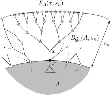
Figure 1: (adapted from [ČTW11]) The point $x\in\partial_{\mathcal{G}_{n}}A$ is a good vertex at the boundary of $A$, the points in $F_{A}(x,s_{n})$ are marked grey.

For $A\subsetneq{\mathcal{G}_{n}}$ non-empty we set

$$G_{A}\coloneqq\{\text{good vertices at the boundary of $A$}\}.$$ (2.29)

We are now ready to state Proposition 2.7. Observe the analogies between its statement and (2.24).

Proposition 2.7.

For every $b,b^{\prime}>0$ there exists $c_{b,b^{\prime}}>0$ such that for $n\geq 1$, $A\subseteq{\mathcal{G}_{n}}$ non-empty with $|A|\leq b\ln(N_{n})$, $x\in G_{A}$ and on the event $\big{\{}\sup_{z\in A}|\Psi_{\mathcal{G}_{n}}(z)|\leq b^{\prime}\sqrt{\ln(N_{n})}\big{\}}$ it holds

$$\Big{|}\mathbb{E}^{\mathcal{G}_{n}}\big{[}\Psi_{\mathcal{G}_{n}}(x)\,\big{|}\,\sigma(\Psi_{\mathcal{G}_{n}}(y),y\in A)\big{]}-\frac{1}{d-1}\Psi_{\mathcal{G}_{n}}(\overline{x})\Big{|} \leq c_{b,b^{\prime}}(\ln(N_{n}))^{-2},$$ (2.30)

$$\Big{|}\textup{Var}_{\mathbb{P}^{\mathcal{G}_{n}}}\big{(}\Psi_{\mathcal{G}_{n}}(x)\,\big{|}\,\sigma(\Psi_{\mathcal{G}_{n}}(y),y\in A)\big{)}-\frac{d}{d-1}\Big{|} \leq c_{b,b^{\prime}}(\ln(N_{n}))^{-3}.$$ (2.31)

Recall that $\overline{x}\in A$ denotes the unique neighbour of $x$ in $A$ (see (2.26)).

To show Proposition 2.7 and conclude this section we will manipulate the explicit expressions for the conditional expectation and variance obtained in Lemma 2.6. In these expressions one considers the hitting time of $A$ for the simple random walk on ${\mathcal{G}_{n}}$ and in the proof of Proposition 2.7 we will look at different situations for when the hitting happens (see the beginning of the proof of Proposition 2.7 below). Since $x\in G_{A}$ in the statement, the simple random walk started at $x$ has to leave $F_{A}(x,s_{n})$ to hit $A$ and so $P_{x}^{\mathcal{G}_{n}}$-almost surely either $H_{A}=T_{F_{A}(x,s_{n})}$ or $H_{A}>T_{F_{A}(x,s_{n})}$. We will further split the latter case into whether $H_{A}$ happens before or after an additional time

$$t_{n}\coloneqq\frac{1}{\lambda_{\mathcal{G}_{n}}}(\ln(N_{n}))^{2},$$ (2.32)

by which the distribution of the simple random walk is very close to the stationary distribution (here the uniform distribution on ${\mathcal{G}_{n}}$). This follows from e.g. [SC97], Corollary 2.1.5. So in the proof of Proposition 2.7 we will consider the three situations $H_{A}=T_{F_{A}(x,s_{n})}$, $T_{F_{A}(x,s_{n})}<H_{A}<T_{F_{A}(x,s_{n})}+t_{n}$ and $H_{A}\geq T_{F_{A}(x,s_{n})}+t_{n}$ separately. Before that, we collect in Lemma 2.8 some preliminary observations about the simple random walk on ${\mathcal{G}_{n}}$ and subsequently start with the proof of Proposition 2.7. For the rest of this section we will abbreviate $F_{A}\coloneqq F_{A}(x,s_{n})$. It is also convenient to consider the continuous-time simple random walk $(\overline{X}_{t})_{t\geq 0}$. We remind that for the exit time from $U\subseteq{\mathcal{G}_{n}}$ (resp. for the entrance time in $U\subseteq{\mathcal{G}_{n}}$) of this walk we use the same notation $T_{U}$ (resp. $H_{U}$) as for the discrete-time simple random walk.

Lemma 2.8.

For $n\geq 1$, $A\subseteq{\mathcal{G}_{n}}$ non-empty and $x\in G_{A}$ one has

(i) $$\ \,\tfrac{1}{d-1}-c(\ln(N_{n}))^{-7}\leq P_{x}^{\mathcal{G}_{n}}[H_{A}=T_{F_{A}}]\leq\tfrac{1}{d-1}\quad\text{and}\quad E_{x}^{\mathcal{G}_{n}}[T_{F_{A}}]\leq c\ln(N_{n})$$ (2.33)

(ii) $$\ \,P_{x}^{\mathcal{G}_{n}}[H_{A}>T_{F_{A}}]=\sum_{z\in B_{\mathcal{G}_{n}}(A,s_{n})^{\mathsf{c}}}P_{x}^{\mathcal{G}_{n}}[\overline{X}_{T_{F_{A}}}=z,H_{A}>T_{F_{A}}].$$ (2.34)

Moreover, for every $b>0$ there exists $c_{b}>0$ such that for $n\geq 1$, $A\subseteq{\mathcal{G}_{n}}$ non-empty with $|A|\leq b\ln(N_{n})$ and $x\in G_{A}$ one has

(iii) $$\ \,P_{x}^{\mathcal{G}_{n}}[T_{F_{A}}<H_{A}<T_{F_{A}}+t_{n}]\leq c_{b}(\ln(N_{n}))^{-5}$$ (2.35)

(iv) $$\ \,\sum_{w\in{\mathcal{G}_{n}}}\big{|}P_{z}^{\mathcal{G}_{n}}[\overline{X}_{t_{n}}=w,H_{A}\geq t_{n}]-\tfrac{1}{N_{n}}\big{|}\leq c_{b}(\ln(N_{n}))^{-5}\quad\text{for }z\in{\mathcal{G}_{n}}$$ (2.36)

(v) $$\ \,\Big{|}\tfrac{E_{x}^{\mathcal{G}_{n}}[H_{A}]}{E_{\pi}^{\mathcal{G}_{n}}[H_{A}]}-P_{x}^{\mathcal{G}_{n}}[H_{A}>T_{F_{A}}]\Big{|}\leq c_{b}(\ln(N_{n}))^{-3}.$$ (2.37)

Proof.

Due to (2.27), the probability $P_{x}^{\mathcal{G}_{n}}[H_{A}=T_{F_{A}}]$ is equal to the probability that a (discrete-time) random walk on $\mathbb{Z}$ started at 1 and jumping with probability $\frac{d-1}{d}$ to the right and $\frac{1}{d}$ to the left hits 0 before hitting $s_{n}+1$. Similarly, $E_{x}^{\mathcal{G}_{n}}[T_{F_{A}}]$ is equal to the expected time until this random walk hits 0 or $s_{n}+1$. Thus (see e.g. [Fel68], (2.4) and (3.4) in Chapter 14) it holds

$$\begin{split}&P_{x}^{\mathcal{G}_{n}}[H_{A}=T_{F_{A}}]=1-\tfrac{d-2}{d-1}(1-(\tfrac{1}{d-1})^{s_{n}+1})^{-1}\leq 1-\tfrac{d-2}{d-1}=\tfrac{1}{d-1},\\ &E_{x}^{\mathcal{G}_{n}}[T_{F_{A}}]=\tfrac{d}{d-2}\Big{(}(s_{n}+1)\tfrac{d-2}{d-1}\frac{1}{1-(\frac{1}{d-1})^{s_{n}+1}}-1\Big{)}\leq 2\tfrac{d}{d-1}(s_{n}+1)\overset{\eqref{471}}{\leq}c\ln(N_{n}).\end{split}$$

Since $(1-(\frac{1}{d-1})^{s_{n}+1})^{-1}\leq(1-(\log_{d-1}(N_{n}))^{-8})^{-1}\leq 1+c(\ln(N_{n}))^{-7}$, one also has $P_{x}^{\mathcal{G}_{n}}[H_{A}=T_{F_{A}}]\geq 1-\tfrac{d-2}{d-1}(1+c(\ln(N_{n}))^{-7})\geq\tfrac{1}{d-1}-c(\ln(N_{n}))^{-7}$. Thus (2.33) is shown.

To see (2.34) observe that on the event $\{H_{A}>T_{F_{A}}\}$, at the moment the simple random walk started at $x$ leaves $F_{A}$, it is in some $z\in\partial_{\mathcal{G}_{n}}F_{A}\cap B_{\mathcal{G}_{n}}(A,s_{n})^{\mathsf{c}}$ (note that indeed $z\notin B_{\mathcal{G}_{n}}(A,s_{n})$ since else there would exist a path like those excluded by (2.28)). In other words,

$$P_{x}^{\mathcal{G}_{n}}\text{-almost surely }\overline{X}_{T_{F_{A}}}\in\partial_{\mathcal{G}_{n}}F_{A}\cap B_{\mathcal{G}_{n}}(A,s_{n})^{\mathsf{c}}\text{ on the event }\{H_{A}>T_{F_{A}}\}.$$ (2.38)

This shows (2.34). To derive (2.35) we apply the strong Markov property of simple random walk for time $T_{F_{A}}$ and obtain for $n\geq 1$

$$P_{x}^{\mathcal{G}_{n}}[T_{F_{A}}<H_{A}<T_{F_{A}}+t_{n}]\overset{\eqref{0003}}{\leq}\sup_{z\in B_{\mathcal{G}_{n}}(A,s_{n})^{\mathsf{c}}}P_{z}^{\mathcal{G}_{n}}[H_{A}<t_{n}].$$ (2.39)

Roughly speaking, the right hand side of (2.39) is small since it is difficult for the simple random walk to hit $A$ within time $t_{n}$ because it starts at distance larger than $s_{n}$ from $A$ and the environment is nearly treelike (see $\eqref{1}$). More precisely, we can apply [ČTW11], Lemma 3.4 (for $T\coloneqq t_{n}$, $r\coloneqq 0$, $s\coloneqq s_{n}$ and using (0.2)) to find $c,c^{\prime}>0$ such that for $z\in B_{\mathcal{G}_{n}}(A,s_{n})^{\mathsf{c}}$ one has for $n\geq 1$

$$P_{z}^{\mathcal{G}_{n}}[H_{A}<t_{n}]\leq\sum_{y\in A}P_{z}^{\mathcal{G}_{n}}[H_{y}<t_{n}]\leq|A|\big{(}ct_{n}(d-1)^{-s_{n}}+e^{-c^{\prime}t_{n}}\big{)}\overset{\eqref{471}}{\leq}c_{b}(\ln(N_{n}))^{-5},$$

where the last inequality also uses the assumption on $A$, (2.32) and (0.3). This combined with (2.39) gives (2.35).

For (2.36) the idea is that on the event $\{H_{A}\geq t_{n}\}$ the simple random walk started at $z$ has, roughly speaking, reached the stationary distribution by time $t_{n}$ without having hit $A$. We observe that for $z,w\in{\mathcal{G}_{n}}$ one has

$$\big{|}P_{z}^{\mathcal{G}_{n}}[\overline{X}_{t_{n}}=w,H_{A}\geq t_{n}]-\tfrac{1}{N_{n}}\big{|} \overset{\phantom{\eqref{97}}}{\leq}P_{z}^{\mathcal{G}_{n}}[\overline{X}_{t_{n}}=w,H_{A}<t_{n}]+\big{|}P_{z}^{\mathcal{G}_{n}}[\overline{X}_{t_{n}}=w]-\tfrac{1}{N_{n}}\big{|}$$

$$\overset{\,\ (*)\ \,}{\leq}P_{z}^{\mathcal{G}_{n}}[\overline{X}_{t_{n}}=w,H_{A}<t_{n}]+\exp(-\lambda_{\mathcal{G}_{n}}t_{n})$$

$$\overset{\eqref{97}}{=}P_{z}^{\mathcal{G}_{n}}[\overline{X}_{t_{n}}=w,H_{A}<t_{n}]+\exp(-(\ln(N_{n}))^{2}),$$

where in $(*)$ we apply [SC97], Corollary 2.1.5. Hence for $n\geq 1$, $z\in{\mathcal{G}_{n}}$, one has

$$\begin{split}&\sum_{w\in{\mathcal{G}_{n}}}\big{|}P_{z}^{\mathcal{G}_{n}}[\overline{X}_{t_{n}}=w,H_{A}\geq t_{n}]-\tfrac{1}{N_{n}}\big{|}\leq P_{z}^{\mathcal{G}_{n}}[H_{A}<t_{n}]+N_{n}\exp(-(\ln(N_{n}))^{2}),\end{split}$$

which together with the above estimate on $P_{z}^{\mathcal{G}_{n}}[H_{A}<t_{n}]$ gives (2.36). It remains to show (2.37). We start by computing (using also (3.20) of [ČTW11] in the second inequality)

$$\frac{E_{x}^{\mathcal{G}_{n}}[H_{A}\boldsymbol{1}_{H_{A}=T_{F_{A}}}]}{E_{\pi}^{\mathcal{G}_{n}}[H_{A}]}\leq\frac{E_{x}^{\mathcal{G}_{n}}[T_{F_{A}}]}{E_{\pi}^{\mathcal{G}_{n}}[H_{A}]}\overset{\eqref{0007}}{\leq}c\ln(N_{n})\frac{4|A|}{N_{n}}\leq\frac{c_{b}(\ln(N_{n}))^{2}}{N_{n}}.$$ (2.40)

Now by (2.38) and the strong Markov property of simple random walk for time $T_{F_{A}}$ one has $E_{x}^{\mathcal{G}_{n}}[H_{A}\boldsymbol{1}_{H_{A}>T_{F_{A}}}]=\sum_{z\in B_{\mathcal{G}_{n}}(A,s_{n})^{\mathsf{c}}}P_{x}^{\mathcal{G}_{n}}[\overline{X}_{T_{F_{A}}}=z,H_{A}>T_{F_{A}}]E_{z}^{\mathcal{G}_{n}}[H_{A}]$. This combined with (2.34) shows

$$\begin{split}&\bigg{|}\frac{E_{x}^{\mathcal{G}_{n}}[H_{A}\boldsymbol{1}_{H_{A}>T_{F_{A}}}]}{E_{\pi}^{\mathcal{G}_{n}}[H_{A}]}-P_{x}^{\mathcal{G}_{n}}[H_{A}>T_{F_{A}}]\bigg{|}\leq\sup_{z\in B_{\mathcal{G}_{n}}(A,s_{n})^{\mathsf{c}}}\bigg{|}\frac{E_{z}^{\mathcal{G}_{n}}[H_{A}]}{E_{\pi}^{\mathcal{G}_{n}}[H_{A}]}-1\bigg{|}.\end{split}$$ (2.41)

By [ČTW11], Proposition 3.5, we can bound the absolute value on the right hand side of (2.41) by $c|A|(d-1)^{-s_{n}}(\ln(N_{n}))^{4}\leq c_{b}(\ln(N_{n}))^{-3}$. Since $P_{x}^{\mathcal{G}_{n}}$-almost surely either $H_{A}=T_{F_{A}}$ or $H_{A}>T_{F_{A}}$, the combination of (2.40) and (2.41) concludes the proof. ∎

Proof of Proposition 2.7.

We start with the basic observation that by (2.16) one has $\big{|}\mathbb{E}^{\mathcal{G}_{n}}\big{[}\Psi_{\mathcal{G}_{n}}(x)\,\big{|}\,\sigma(\Psi_{\mathcal{G}_{n}}(y),y\in A)\big{]}-\frac{1}{d-1}\Psi_{\mathcal{G}_{n}}(\overline{x})\big{|}\leq U_{A,x}^{\mathcal{G}_{n}}+V_{A,x}^{\mathcal{G}_{n}}+W_{A,x}^{\mathcal{G}_{n}}$, where

$$\begin{split}U_{A,x}^{\mathcal{G}_{n}}&\coloneqq\Big{|}E_{x}^{\mathcal{G}_{n}}\big{[}\Psi_{\mathcal{G}_{n}}(\overline{X}_{H_{A}})\boldsymbol{1}_{\{H_{A}=T_{F_{A}}\}}\big{]}-\tfrac{1}{d-1}\Psi_{\mathcal{G}_{n}}(\overline{x})\Big{|},\\ V_{A,x}^{\mathcal{G}_{n}}&\coloneqq\big{|}E_{x}^{\mathcal{G}_{n}}\big{[}\Psi_{\mathcal{G}_{n}}(\overline{X}_{H_{A}})\boldsymbol{1}_{\{T_{F_{A}}<H_{A}<T_{F_{A}}+t_{n}\}}\big{]}\big{|},\\ W_{A,x}^{\mathcal{G}_{n}}&\coloneqq\Big{|}E_{x}^{\mathcal{G}_{n}}\big{[}\Psi_{\mathcal{G}_{n}}(\overline{X}_{H_{A}})\boldsymbol{1}_{\{H_{A}\geq T_{F_{A}}+t_{n}\}}\big{]}-\tfrac{E_{x}^{\mathcal{G}_{n}}[H_{A}]}{E_{\pi}^{\mathcal{G}_{n}}[H_{A}]}E_{\pi}^{\mathcal{G}_{n}}\big{[}\Psi_{\mathcal{G}_{n}}(\overline{X}_{H_{A}})\big{]}\Big{|}.\end{split}$$

Hence the proof of (2.30) follows once we show that

there exists $$c_{b,b^{\prime}}>0 n\geq 1 A\subseteq{\mathcal{G}_{n}} |A|\leq b\ln(N_{n}) x\in G_{A} \big{\{}\textstyle\sup_{z\in A}|\Psi_{\mathcal{G}_{n}}(z)|\leq b^{\prime}\sqrt{\ln(N_{n})}\big{\}} U_{A,x}^{\mathcal{G}_{n}}+V_{A,x}^{\mathcal{G}_{n}}+W_{A,x}^{\mathcal{G}_{n}}\leq c_{b,b^{\prime}}(\ln(N_{n}))^{-2}$$ such that for , non-empty with , and on the event one has . (2.42)

Similarly we have $\big{|}\textup{Var}_{\mathbb{P}^{\mathcal{G}_{n}}}\big{(}\Psi_{\mathcal{G}_{n}}(x)\,\big{|}\,\sigma(\Psi_{\mathcal{G}_{n}}(y),y\in A)\big{)}-\frac{d}{d-1}\big{|}\leq\overline{U}_{A,x}^{\mathcal{G}_{n}}+\overline{V}_{A,x}^{\mathcal{G}_{n}}+\overline{W}_{A,x}^{\mathcal{G}_{n}}$ by (2.17), where

$$\begin{split}\overline{U}_{A,x}^{\mathcal{G}_{n}}&\coloneqq\Big{|}G_{\mathcal{G}_{n}}(x,x)-E_{x}^{\mathcal{G}_{n}}\big{[}G_{\mathcal{G}_{n}}(X_{H_{A}},x)\boldsymbol{1}_{\{H_{A}=T_{F_{A}}\}}\big{]}-\tfrac{d}{d-1}\Big{|},\\ \overline{V}_{A,x}^{\mathcal{G}_{n}}&\coloneqq E_{x}^{\mathcal{G}_{n}}\big{[}G_{\mathcal{G}_{n}}(X_{H_{A}},x)\boldsymbol{1}_{\{T_{F_{A}}<H_{A}<T_{F_{A}}+t_{n}\}}\big{]},\\ \overline{W}_{A,x}^{\mathcal{G}_{n}}&\coloneqq\Big{|}E_{x}^{\mathcal{G}_{n}}\big{[}G_{\mathcal{G}_{n}}(X_{H_{A}},x)\boldsymbol{1}_{\{H_{A}\geq T_{F_{A}}+t_{n}\}}\big{]}-\tfrac{E_{x}^{\mathcal{G}_{n}}[H_{A}]}{E_{\pi}^{\mathcal{G}_{n}}[H_{A}]}E_{\pi}^{\mathcal{G}_{n}}[G_{\mathcal{G}_{n}}(X_{H_{A}},x)]\Big{|}.\end{split}$$

Thus the proof of (2.31) follows once we show that

there exists $$c_{b}>0 n\geq 1 A\subseteq{\mathcal{G}_{n}} |A|\leq b\ln(N_{n}) x\in G_{A} \overline{U}_{A,x}^{\mathcal{G}_{n}}+\overline{V}_{A,x}^{\mathcal{G}_{n}}+\overline{W}_{A,x}^{\mathcal{G}_{n}}\leq c_{b}(\ln(N_{n}))^{-3}$$ such that for , non-empty with and one has . (2.43)

It remains to show (2.42) and (2.43). For (2.42) we bound the three terms $U_{A,x}^{\mathcal{G}_{n}}$, $V_{A,x}^{\mathcal{G}_{n}}$ and $W_{A,x}^{\mathcal{G}_{n}}$ separately. On $\{H_{A}=T_{F_{A}}\}$ one has $P_{x}^{\mathcal{G}_{n}}$-almost surely $\Psi_{\mathcal{G}_{n}}(\overline{X}_{H_{A}})=\Psi_{\mathcal{G}_{n}}(\overline{x})$ due to $x\in G_{A}$. Therefore we deduce $U_{A,x}^{\mathcal{G}_{n}}=|\Psi_{\mathcal{G}_{n}}(\overline{x})|\cdot\big{|}P_{x}^{\mathcal{G}_{n}}[H_{A}=T_{F_{A}}]-\tfrac{1}{d-1}\big{|}\leq b^{\prime}\sqrt{\ln(N_{n})}c(\ln(N_{n}))^{-7}$ by (2.33), where in the last inequality we also use that $\overline{x}\in A$. This shows $U_{A,x}^{\mathcal{G}_{n}}\leq c_{b^{\prime}}(\ln(N_{n}))^{-6}$.

We turn to $V_{A,x}^{\mathcal{G}_{n}}$. By (2.35) we have $V_{A,x}^{\mathcal{G}_{n}}\leq\sup_{y\in A}|\Psi_{\mathcal{G}_{n}}(y)|\cdot P_{x}^{\mathcal{G}_{n}}[T_{F_{A}}<H_{A}<T_{F_{A}}+t_{n}]\leq b^{\prime}\sqrt{\ln(N_{n})}c_{b}(\ln(N_{n}))^{-5}$. This shows $V_{A,x}^{\mathcal{G}_{n}}\leq c_{b,b^{\prime}}(\ln(N_{n}))^{-4}$.

Finally, we consider $W_{A,x}^{\mathcal{G}_{n}}$. Let us define

$$\begin{split}Y_{A,x}^{\mathcal{G}_{n}}&\coloneqq\Big{|}\tfrac{E_{x}^{\mathcal{G}_{n}}[H_{A}]}{E_{\pi}^{\mathcal{G}_{n}}[H_{A}]}-P_{x}^{\mathcal{G}_{n}}[H_{A}>T_{F_{A}}]\Big{|},\\ Z_{A,x}^{\mathcal{G}_{n}}&\coloneqq\Big{|}E_{x}^{\mathcal{G}_{n}}\big{[}\Psi_{\mathcal{G}_{n}}(\overline{X}_{H_{A}})\boldsymbol{1}_{\{H_{A}\geq T_{F_{A}}+t_{n}\}}\big{]}-P_{x}^{\mathcal{G}_{n}}[H_{A}>T_{F_{A}}]E_{\pi}^{\mathcal{G}_{n}}\big{[}\Psi_{\mathcal{G}_{n}}(\overline{X}_{H_{A}})\big{]}\Big{|}.\end{split}$$ (2.44)

By adding and subtracting $\tfrac{1}{P_{x}^{\mathcal{G}_{n}}[H_{A}>T_{F_{A}}]}\tfrac{E_{x}^{\mathcal{G}_{n}}[H_{A}]}{E_{\pi}^{\mathcal{G}_{n}}[H_{A}]}E_{x}^{\mathcal{G}_{n}}\big{[}\Psi_{\mathcal{G}_{n}}(\overline{X}_{H_{A}})\boldsymbol{1}_{\{H_{A}\geq T_{F_{A}}+t_{n}\}}\big{]}$ inside the expression for $W_{A,x}^{\mathcal{G}_{n}}$ we obtain

$$W_{A,x}^{\mathcal{G}_{n}}\leq\tfrac{|E_{x}^{\mathcal{G}_{n}}[\Psi_{\mathcal{G}_{n}}(\overline{X}_{H_{A}})\boldsymbol{1}_{\{H_{A}\geq T_{F_{A}}+t_{n}\}}]|}{P_{x}^{\mathcal{G}_{n}}[H_{A}>T_{F_{A}}]}\,Y_{A,x}^{\mathcal{G}_{n}}+\tfrac{1}{P_{x}^{\mathcal{G}_{n}}[H_{A}>T_{F_{A}}]}\tfrac{E_{x}^{\mathcal{G}_{n}}[H_{A}]}{E_{\pi}^{\mathcal{G}_{n}}[H_{A}]}Z_{A,x}^{\mathcal{G}_{n}}.$$ (2.45)

To the first term on the right hand side of (2.45) we apply $P_{x}^{\mathcal{G}_{n}}[H_{A}>T_{F_{A}}]\geq\frac{d-2}{d-1}$ (by (2.33)) as well as (2.37) and the assumption on the supremum of $\Psi_{\mathcal{G}_{n}}$ on $A$. For the second term we first observe (2.37) and then again use $P_{x}^{\mathcal{G}_{n}}[H_{A}>T_{F_{A}}]\geq\frac{d-2}{d-1}$. In this way we obtain

$$W_{A,x}^{\mathcal{G}_{n}}\leq c_{b,b^{\prime}}(\ln(N_{n}))^{-2}+(1+c_{b}(\ln(N_{n}))^{-3})Z_{A,x}^{\mathcal{G}_{n}}.$$ (2.46)

We proceed to bound $Z_{A,x}^{\mathcal{G}_{n}}$. By (2.38) and the strong Markov property for time $T_{F_{A}}$ it holds

$$E_{x}^{\mathcal{G}_{n}}\big{[}\Psi_{\mathcal{G}_{n}}(\overline{X}_{H_{A}})\boldsymbol{1}_{\{H_{A}\geq T_{F_{A}}+t_{n}\}}\big{]}$$

$$\qquad\qquad=\sum_{z\in B_{\mathcal{G}_{n}}(A,s_{n})^{\mathsf{c}}}P_{x}^{\mathcal{G}_{n}}[\overline{X}_{T_{F_{A}}}=z,H_{A}>T_{F_{A}}]E_{z}^{\mathcal{G}_{n}}\big{[}\Psi_{\mathcal{G}_{n}}(\overline{X}_{H_{A}})\boldsymbol{1}_{\{H_{A}\geq t_{n}\}}\big{]}.$$

This combined with (2.34) implies $Z_{A,x}^{\mathcal{G}_{n}}\leq\sup_{z\in B_{\mathcal{G}_{n}}(A,s_{n})^{\mathsf{c}}}\big{|}E_{z}^{\mathcal{G}_{n}}[\Psi_{\mathcal{G}_{n}}(\overline{X}_{H_{A}})\boldsymbol{1}_{\{H_{A}\geq t_{n}\}}]-E_{\pi}^{\mathcal{G}_{n}}[\Psi_{\mathcal{G}_{n}}(\overline{X}_{H_{A}})]\big{|}$. Now for $z\in B_{\mathcal{G}_{n}}(A,s_{n})^{\mathsf{c}}$, by the Markov property applied at time $t_{n}$ and the definition of $E_{\pi}^{\mathcal{G}_{n}}$,

$$\begin{split}&\big{|}E_{z}^{\mathcal{G}_{n}}[\Psi_{\mathcal{G}_{n}}(\overline{X}_{H_{A}})\boldsymbol{1}_{\{H_{A}\geq t_{n}\}}]-E_{\pi}^{\mathcal{G}_{n}}[\Psi_{\mathcal{G}_{n}}(\overline{X}_{H_{A}})]\big{|}\\ &\leq\sum_{w\in{\mathcal{G}_{n}}}\big{|}E_{w}^{\mathcal{G}_{n}}[\Psi_{\mathcal{G}_{n}}(\overline{X}_{H_{A}})]\big{|}\cdot\big{|}P_{z}^{\mathcal{G}_{n}}[\overline{X}_{t_{n}}=w,H_{A}\geq t_{n}]-\tfrac{1}{N_{n}}\big{|}\overset{\eqref{0006}}{\leq}c_{b,b^{\prime}}(\ln(N_{n}))^{-4},\end{split}$$

where in the last inequality we also use the assumption on the supremum of $\Psi_{\mathcal{G}_{n}}$ on $A$. All in all we have shown $Z_{A,x}^{\mathcal{G}_{n}}\leq c_{b,b^{\prime}}(\ln(N_{n}))^{-4}$. Thus by (2.46) we deduce $W_{A,x}^{\mathcal{G}_{n}}\leq c_{b,b^{\prime}}(\ln(N_{n}))^{-2}$ and the proof of (2.42) is complete.

We come to the proof of (2.43) for which we bound the three terms $\overline{U}_{A,x}^{\mathcal{G}_{n}}$, $\overline{V}_{A,x}^{\mathcal{G}_{n}}$ and $\overline{W}_{A,x}^{\mathcal{G}_{n}}$ separately. For $\overline{U}_{A,x}^{\mathcal{G}_{n}}$ we first note that one has $E_{x}^{\mathcal{G}_{n}}\big{[}G_{\mathcal{G}_{n}}(X_{H_{A}},x)\boldsymbol{1}_{\{H_{A}=T_{F_{A}}\}}\big{]}=E_{x}^{\mathcal{G}_{n}}\big{[}G_{\mathcal{G}_{n}}(X_{T_{F_{A}}},x)\boldsymbol{1}_{\{H_{A}=T_{F_{A}}\}}\big{]}=E_{x}^{\mathcal{G}_{n}}\big{[}G_{\mathcal{G}_{n}}(X_{T_{F_{A}}},x)\big{]}-E_{x}^{\mathcal{G}_{n}}\big{[}G_{\mathcal{G}_{n}}(X_{T_{F_{A}}},x)\boldsymbol{1}_{\{H_{A}>T_{F_{A}}\}}\big{]}$. By (2.38), on the event $\{H_{A}>T_{F_{A}}\}$ the simple random walk started at $x$ is at distance $s_{n}$ from $x$ when it leaves $F_{A}$. Therefore

$$E_{x}^{\mathcal{G}_{n}}\big{[}G_{\mathcal{G}_{n}}(X_{T_{F_{A}}},x)\boldsymbol{1}_{\{H_{A}>T_{F_{A}}\}}\big{]}\leq\sup_{z\in S_{\mathcal{G}_{n}}(x,s_{n})}\!G_{\mathcal{G}_{n}}(z,x)\,\underbrace{P_{x}^{\mathcal{G}_{n}}[H_{A}>T_{F_{A}}]}_{\leq 1}\stackrel{{\scriptstyle[}}{{\eqref{}}}{471}]{\eqref{30}}{\leq}c(\ln(N_{n}))^{-8}.$$

Thus we have

$$\begin{split}\overline{U}_{A,x}^{\mathcal{G}_{n}}&\overset{\phantom{\eqref{1.7}}}{\leq}\Big{|}G_{\mathcal{G}_{n}}(x,x)-E_{x}^{\mathcal{G}_{n}}\big{[}G_{\mathcal{G}_{n}}(X_{T_{F_{A}}},x)\big{]}-\tfrac{d}{d-1}\Big{|}+c(\ln(N_{n}))^{-8}\\ &\stackrel{{\scriptstyle[}}{{\eqref{}}}{0007}]{\eqref{1.7}}{\leq}\big{|}g_{\mathcal{G}_{n}}^{F_{A}}(x,x)-\tfrac{d}{d-1}\big{|}+\tfrac{c\ln(N_{n})}{N_{n}}+c(\ln(N_{n}))^{-8}.\end{split}$$ (2.47)

Note that by assumption $\mathtt{tx}(F_{A})=0$. So if we define $B\coloneqq B_{\mathbb{T}_{d}}^{+}({\textup{o}},s_{n})\setminus\{{\textup{o}}\}\subseteq{\mathbb{T}_{d}}$ and take $x_{1}\in S_{\mathbb{T}_{d}}^{+}({\textup{o}},1)$, then by definition we have $g_{\mathcal{G}_{n}}^{F_{A}}(x,x)=g_{\mathbb{T}_{d}}^{B}(x_{1},x_{1})$. From (1.7) we see that

$$g_{\mathbb{T}_{d}}^{B}(x_{1},x_{1}) =g_{\mathbb{T}_{d}}(x_{1},x_{1})-E_{x_{1}}^{\mathbb{T}_{d}}[g_{\mathbb{T}_{d}}(X_{T_{B}},x_{1})]$$

$$=g_{\mathbb{T}_{d}}(x_{1},x_{1})-g_{\mathbb{T}_{d}}({\textup{o}},x_{1})P_{x_{1}}^{\mathbb{T}_{d}}[H_{\textup{o}}=T_{B}]-g_{\mathbb{T}_{d}}(z,x_{1})P_{x_{1}}^{\mathbb{T}_{d}}[H_{\textup{o}}>T_{B}]$$

for any fixed $z\in S_{\mathbb{T}_{d}}^{+}({\textup{o}},s_{n}+1)$. By (1.6) this shows that

$$g_{\mathbb{T}_{d}}^{B}(x_{1},x_{1})=\frac{d-1}{d-2}-\frac{d-1}{d-2}\frac{1}{d-1}P_{x}^{\mathcal{G}_{n}}[H_{A}=T_{F_{A}}]-\frac{d-1}{d-2}\big{(}\frac{1}{d-1}\big{)}^{s_{n}}P_{x}^{\mathcal{G}_{n}}[H_{A}>T_{F_{A}}].$$

So we have obtained

$$\begin{split}\big{|}g_{\mathcal{G}_{n}}^{F_{A}}(x,x)-\tfrac{d}{d-1}\big{|}&\overset{\phantom{\eqref{0007}}}{\leq}\big{|}\tfrac{d-1}{d-2}-\tfrac{1}{d-2}P_{x}^{\mathcal{G}_{n}}[H_{A}=T_{F_{A}}]-\tfrac{d}{d-1}\big{|}+\tfrac{d-1}{d-2}\big{(}\tfrac{1}{d-1}\big{)}^{s_{n}}P_{x}^{\mathcal{G}_{n}}[H_{A}>T_{F_{A}}]\\ &\stackrel{{\scriptstyle[}}{{\eqref{}}}{471}]{\eqref{0007}}{\leq}\tfrac{1}{d-2}c(\ln(N_{n}))^{-7}+c(\ln(N_{n}))^{-8}.\end{split}$$

This, together with (2.47) shows $\overline{U}_{A,x}^{\mathcal{G}_{n}}\leq c(\ln(N_{n}))^{-7}$.

We turn to $\overline{V}_{A,x}^{\mathcal{G}_{n}}$. By (1.22) there exists $c>0$ such that $\sup_{y,z\in{\mathcal{G}_{n}}}G_{\mathcal{G}_{n}}(y,z)\leq c$. Therefore $\overline{V}_{A,x}^{\mathcal{G}_{n}}\leq c\,P_{x}^{\mathcal{G}_{n}}[T_{F_{A}}<H_{A}<T_{F_{A}}+t_{n}]$ and so (2.35) implies $\overline{V}_{A,x}^{\mathcal{G}_{n}}\leq c_{b}(\ln(N_{n}))^{-5}$.

Finally, we consider $\overline{W}_{A,x}^{\mathcal{G}_{n}}$. Let us define

$$\overline{Z}_{A,x}^{\mathcal{G}_{n}}\coloneqq\Big{|}E_{x}^{\mathcal{G}_{n}}\big{[}G_{\mathcal{G}_{n}}(X_{H_{A}},x)\boldsymbol{1}_{\{H_{A}\geq T_{F_{A}}+t_{n}\}}\big{]}-P_{x}^{\mathcal{G}_{n}}[H_{A}>T_{F_{A}}]E_{\pi}^{\mathcal{G}_{n}}[G_{\mathcal{G}_{n}}(X_{H_{A}},x)]\Big{|}$$

and recall $Y_{A,x}^{\mathcal{G}_{n}}$ from (2.44). Inside $\overline{W}_{A,x}^{\mathcal{G}_{n}}$ we can add and subtract $\tfrac{1}{P_{x}^{\mathcal{G}_{n}}[H_{A}>T_{F_{A}}]}\tfrac{E_{x}^{\mathcal{G}_{n}}[H_{A}]}{E_{\pi}^{\mathcal{G}_{n}}[H_{A}]}\cdot E_{x}^{\mathcal{G}_{n}}\big{[}G_{\mathcal{G}_{n}}(X_{H_{A}},x)\boldsymbol{1}_{\{H_{A}\geq T_{F_{A}}+t_{n}\}}\big{]}$ to obtain

$$\overline{W}_{A,x}^{\mathcal{G}_{n}}\leq\tfrac{E_{x}^{\mathcal{G}_{n}}[G_{\mathcal{G}_{n}}(X_{H_{A}},x)\boldsymbol{1}_{\{H_{A}\geq T_{F_{A}}+t_{n}\}}]}{P_{x}^{\mathcal{G}_{n}}[H_{A}>T_{F_{A}}]}\,Y_{A,x}^{\mathcal{G}_{n}}+\tfrac{1}{P_{x}^{\mathcal{G}_{n}}[H_{A}>T_{F_{A}}]}\tfrac{E_{x}^{\mathcal{G}_{n}}[H_{A}]}{E_{\pi}^{\mathcal{G}_{n}}[H_{A}]}\overline{Z}_{A,x}^{\mathcal{G}_{n}}.\\$$ (2.48)

To the first term on the right hand side of (2.48) we apply $P_{x}^{\mathcal{G}_{n}}[H_{A}>T_{F_{A}}]\geq\frac{d-2}{d-1}$ (by (2.33)) as well as (2.37) and $\sup_{y,z\in{\mathcal{G}_{n}}}G_{\mathcal{G}_{n}}(y,z)\leq c$ (by (1.22)). For the second term we first observe (2.37) and then again use $P_{x}^{\mathcal{G}_{n}}[H_{A}>T_{F_{A}}]\geq\frac{d-2}{d-1}$. In this way we obtain

$$\overline{W}_{A,x}^{\mathcal{G}_{n}}\leq c_{b}(\ln(N_{n}))^{-3}+(1+c_{b}(\ln(N_{n}))^{-3})\overline{Z}_{A,x}^{\mathcal{G}_{n}}.$$ (2.49)

We proceed to bound $\overline{Z}_{A,x}^{\mathcal{G}_{n}}$. By (2.38) and the strong Markov property it holds

$$E_{x}^{\mathcal{G}_{n}}\big{[}G_{\mathcal{G}_{n}}(X_{H_{A}},x)\boldsymbol{1}_{\{H_{A}\geq T_{F_{A}}+t_{n}\}}\big{]}$$

$$\qquad\qquad=\sum_{z\in B_{\mathcal{G}_{n}}(A,s_{n})^{\mathsf{c}}}P_{x}^{\mathcal{G}_{n}}[\overline{X}_{T_{F_{A}}}=z,H_{A}>T_{F_{A}}]E_{z}^{\mathcal{G}_{n}}[G_{\mathcal{G}_{n}}(X_{H_{A}},x)\boldsymbol{1}_{\{H_{A}\geq t_{n}\}}].$$

This combined with (2.34) gives $\overline{Z}_{A,x}^{\mathcal{G}_{n}}\leq\sup_{z\in B_{\mathcal{G}_{n}}(A,s_{n})^{\mathsf{c}}}\big{|}E_{z}^{\mathcal{G}_{n}}[G_{\mathcal{G}_{n}}(X_{H_{A}},x)\boldsymbol{1}_{\{H_{A}\geq t_{n}\}}]-E_{\pi}^{\mathcal{G}_{n}}[G_{\mathcal{G}_{n}}(X_{H_{A}},x)]\big{|}$. Now for $z\in B_{\mathcal{G}_{n}}(A,s_{n})^{\mathsf{c}}$, by the Markov property applied at time $t_{n}$ and the definition of $E_{\pi}^{\mathcal{G}_{n}}$,

$$\begin{split}&\big{|}E_{z}^{\mathcal{G}_{n}}[G_{\mathcal{G}_{n}}(X_{H_{A}},x)\boldsymbol{1}_{\{H_{A}\geq t_{n}\}}]-E_{\pi}^{\mathcal{G}_{n}}[G_{\mathcal{G}_{n}}(X_{H_{A}},x)]\big{|}\\ &\leq\sum_{w\in{\mathcal{G}_{n}}}E_{w}^{\mathcal{G}_{n}}[G_{\mathcal{G}_{n}}(X_{H_{A}},x)]\cdot\big{|}P_{z}^{\mathcal{G}_{n}}[\overline{X}_{t_{n}}=w,H_{A}\geq t_{n}]-\tfrac{1}{N_{n}}\big{|}\overset{\eqref{0006}}{\leq}c_{b}(\ln(N_{n}))^{-5},\end{split}$$

where in the last inequality we again use $\sup_{y,w\in{\mathcal{G}_{n}}}G_{\mathcal{G}_{n}}(y,w)\leq c$ by (1.22). All in all we have shown $\overline{Z}_{A,x}^{\mathcal{G}_{n}}\leq c_{b}(\ln(N_{n}))^{-5}$. Thus by (2.49) we deduce $\overline{W}_{A,x}^{\mathcal{G}_{n}}\leq c_{b}(\ln(N_{n}))^{-3}$ and (2.43) is shown. This concludes the proof of Proposition 2.7 and Section 2.2. ∎

3 Microscopic components in the subcritical phase

We start the analysis of level-set percolation of the zero-average Gaussian free field $\Psi_{\mathcal{G}_{n}}$ on ${\mathcal{G}_{n}}$. The goal of this section is to show (0.8) in the form of Theorem 3.1 below, i.e. the existence of a subcritical phase in which, with high probability for large $n$, level sets of $\Psi_{\mathcal{G}_{n}}$ only have connected components of cardinality at most logarithmic in the size of the graph. To precisely state the result, we recall from the introduction the critical value $h_{\star}$ for level-set percolation of the Gaussian free field $\varphi_{\mathbb{T}_{d}}$ on ${\mathbb{T}_{d}}$ (see (0.7)) and also the notation $E_{\Psi_{\mathcal{G}_{n}}}^{\geq h}$ for the level set of $\Psi_{\mathcal{G}_{n}}$ above level $h\in\mathbb{R}$ (see (0.5)). For $h\in\mathbb{R}$ we further denote by $\mathcal{C}_{\textup{max}}^{{\mathcal{G}_{n}},h}$ an arbitrary connected component of $E_{\Psi_{\mathcal{G}_{n}}}^{\geq h}$ with maximal number of vertices. We will only be interested in its cardinality. Moreover, for $x\in{\mathcal{G}_{n}}$ and $h\in\mathbb{R}$ we define $\mathcal{C}_{x}^{{\mathcal{G}_{n}},h}$ to be the connected component of $E_{\Psi_{\mathcal{G}_{n}}}^{\geq h}$ containing $x$. The main result of this section is

Theorem 3.1.

Let $h>h_{\star}$. Then for all $\kappa>0$ there exist $c_{h,\kappa}>0$ and $K_{h,\kappa}>0$ such that for all $n\geq 1$

$$\mathbb{P}^{\mathcal{G}_{n}}\big{[}|\mathcal{C}_{\textup{max}}^{{\mathcal{G}_{n}},h}|\geq K_{h,\kappa}\ln(N_{n})\big{]}\leq c_{h,\kappa}N_{n}^{-\kappa}.$$

In particular, for some $K_{h}>0$ one has $\lim_{n\to\infty} \mathbb{P}^{\mathcal{G}_{n}}\big{[}|\mathcal{C}_{\textup{max}}^{{\mathcal{G}_{n}},h}|\leq K_{h}\ln(N_{n})\big{]}=1$.

Before explaining the details of the proof of Theorem 3.1, let us make the basic observation that a union bound reduces the problem to show that for $h>h_{\star}$ and for all $\kappa>0$ there exist $c_{h,\kappa}>0$ and $K_{h,\kappa}>0$ such that for all $n\geq 1$ and $x\in{\mathcal{G}_{n}}$

$$\mathbb{P}^{\mathcal{G}_{n}}\big{[}|\mathcal{C}_{x}^{{\mathcal{G}_{n}},h}|\geq K_{h,\kappa}\ln(N_{n})\big{]}\leq c_{h,\kappa}N_{n}^{-1-\kappa}.$$ (3.1)

So it remains to show (3.1). We will make use of a certain exploration process exploring $\mathcal{C}_{x}^{{\mathcal{G}_{n}},h}$ for a fixed $x\in{\mathcal{G}_{n}}$. This will enable us to control $\mathbb{P}^{\mathcal{G}_{n}}\big{[}|\mathcal{C}_{x}^{{\mathcal{G}_{n}},h}|\geq K_{h,\kappa}\ln(N_{n})\big{]}$. A similar approach has for example been followed in [ČTW11] to prove a result analogous to the above Theorem 3.1 but for the vacant set of simple random walk on ${\mathcal{G}_{n}}$ in place of the level set of the zero-average Gaussian free field.

We now give the idea of the proof of (3.1). The details of the exploration process itself are given afterwards. A crucial ingredient is the precise understanding of the conditional distribution of the zero-average Gaussian free field on non-explored vertices given its value on already explored vertices. As we have seen in Proposition 2.7 in Section 2.2, under certain geometric conditions the conditional distribution of $\Psi_{\mathcal{G}_{n}}$ shows strong similarities with the conditional distribution of the Gaussian free field $\varphi_{\mathbb{T}_{d}}$ on ${\mathbb{T}_{d}}$. While exploring $\mathcal{C}_{x}^{{\mathcal{G}_{n}},h}$, the exploration process will separate the vertices found in $\mathcal{C}_{x}^{{\mathcal{G}_{n}},h}$ into a union of rooted disjoint subtrees of ${\mathcal{G}_{n}}$ in which all vertices except for the root satisfy the aforementioned geometric conditions. In this way we reduce the proof of (3.1) to a control of the number of vertices contained in these union of subtrees (Proposition 3.2). As a result from [ČTW11] shows (see also Lemma 3.3), the number of steps the exploration process encounters a situation in which the geometric assumptions fail to be satisfied is not too large. This controls the number of distinct subtrees created by the exploration process because in each subtree there is exactly one vertex which does not satisfy the conditions (its root). Since the other vertices of a subtree satisfy the geometric conditions, we can employ the similarity between the conditional distribution of $\Psi_{\mathcal{G}_{n}}$ and $\varphi_{\mathbb{T}_{d}}$ to couple the zero-average Gaussian free field on each distinct subtree separately with an independent copy of the Gaussian free field $\varphi_{\mathbb{T}_{d}}$ on ${\mathbb{T}_{d}}$ (Lemma 3.4). This translates the question about the number of vertices contained in the disjoint subtrees into the number of vertices contained in connected components of the level set of $\varphi_{\mathbb{T}_{d}}$ (Corollary 3.5). A result from [AČ19] (recalled in (1.14)) about exponential moments of the size of these connected components then ultimately leads to the proof of Proposition 3.2 and hence of (3.1).

We now describe the exploration process exploring $\mathcal{C}_{x}^{{\mathcal{G}_{n}},h}$ for a fixed $x\in{\mathcal{G}_{n}}$ and to facilitate the discussion we include a concrete algorithm implementing it (Algorithm 1). The exploration process is a modified breadth-first-search that discovers the field $\Psi_{\mathcal{G}_{n}}$ on the graph step by step. It employs two queues (a primary and a secondary one) that work in the usual first-in-first-out manner and store the vertices to be explored. The exploration process starts by revealing $\Psi_{\mathcal{G}_{n}}(x)$. The vertices where $\Psi_{\mathcal{G}_{n}}$ has been revealed are called explored and they can be either part of $\mathcal{C}_{x}^{{\mathcal{G}_{n}},h}$ or not. If a vertex is explored and is revealed to be part of $\mathcal{C}_{x}^{{\mathcal{G}_{n}},h}$, then its neighbours which are neither already explored nor already in one of the two queues are added to the primary queue. To avoid ambiguity, we suppose that the vertices of ${\mathcal{G}_{n}}$ are equipped with some ordering and that they are added to the queue following this ordering. Vertices taken out of the primary queue are first checked to be good vertices at the boundary of the so far explored vertices (recall (2.29) and above it for the definition): if they are, the exploration process proceeds with their exploration; if they are not, they are transferred to the secondary queue and their exploration is postponed. The first vertex in the secondary queue is only taken out to be explored if the primary queue is empty.

To formalise this exploration process we now give an algorithm implementing it (see Algorithm 1 below). The algorithm constructs on some auxiliary probability space $(\Omega,\mathcal{A},\mathbb{P})$ a family of random variables $(\psi(z))_{z\in B}$ such that $(\psi(z))_{z\in B}$ under $\mathbb{P}$ has the same distribution as $(\Psi_{\mathcal{G}_{n}}(z))_{z\in B}$ under $\mathbb{P}^{\mathcal{G}_{n}}$. Here $B\subseteq{\mathcal{G}_{n}}$ is some (random) connected set of vertices containing $x$. We use $\mathsf{PQ}$, $\mathsf{SQ}$ and $\mathsf{E}$ to denote the evolving sets of vertices in the primary queue, vertices in the secondary queue and explored vertices during the run of the algorithm. Furthermore, we also keep track of the explored vertices $z\in\mathsf{E}$ for which $\psi(z)\geq h$ using the set $\mathsf{C}\subseteq\mathsf{E}$. Additionally to the exploration, the algorithm aggregates the vertices discovered to be in $\mathsf{C}$ into disjoint subtrees $(\mathsf{T}^{y})_{y}$ of ${\mathcal{G}_{n}}$ indexed by bad vertices $y\in{\mathcal{G}_{n}}$ (meaning they were in $\mathsf{SQ}$ at some point of the algorithm). Moreover, the algorithm stops for one of two reasons: either because both the primary and secondary queue are empty, or because it already discovered that $\mathsf{C}$ has at least size $K_{h,\kappa}\ln(N_{n})$ for some $K_{h,\kappa}$ to be specified later (below (3.22)).

We need some more notation for the algorithm. Let $(\xi_{z})_{z\in{\mathcal{G}_{n}}}$ be i.i.d. standard normal random variables on the auxiliary probability space $(\Omega,\mathcal{A},\mathbb{P})$. For $A\subseteq{\mathcal{G}_{n}}$ non-empty and $u\in{\mathcal{G}_{n}}$ we abbreviate by $a(u,\psi,A)$ the right hand side of (2.16) where $x$ and $\Psi_{\mathcal{G}_{n}}$ are replaced by $u$ and $\psi$. In particular, $a(u,\psi,A)$ is a random variable measurable with respect to $\sigma(\psi(w),w\in A)$. By $b(u,A)$ we abbreviate the right hand side of (2.17) where $x$ is replaced by $u$. For $A=\emptyset$ and $u\in{\mathcal{G}_{n}}$ we define $a(u,\psi,\emptyset)\coloneqq 0$ and $b(u,\emptyset)\coloneqq G_{\mathcal{G}_{n}}(u,u)$. By Lemma 2.6 and the fact that $\psi$ is a Gaussian field, we have that

for $$A\subseteq{\mathcal{G}_{n}} u\in{\mathcal{G}_{n}} a(u,\psi,A)+\xi_{u}\cdot b(u,A)^{\frac{1}{2}} \mathbb{P} \Psi_{\mathcal{G}_{n}}(u) \sigma(\Psi_{\mathcal{G}_{n}}(w),w\in A) \mathbb{P}^{\mathcal{G}_{n}}$$ and the random variable under has the same distribution as conditional on under . (3.2)

The algorithm is as follows:

Algorithm 1

1:set $\mathsf{PQ}\coloneqq\emptyset$, $\mathsf{SQ}\coloneqq\{x\}$, $\mathsf{E}\coloneqq\emptyset$, $\mathsf{C}\coloneqq\emptyset$ and also $\mathsf{T}^{w}\coloneqq\emptyset$ for all $w\in{\mathcal{G}_{n}}$

2:while secondary queue $\mathsf{SQ}$ is not empty do

3:     take vertex $y$ out of $\mathsf{SQ}$

4:     generate the random variable $\psi(y)\coloneqq a(y,\psi,\mathsf{E})+\xi_{y}\cdot b(y,\mathsf{E})^{\frac{1}{2}}$

5:     add $y$ to the set $\mathsf{E}$ of explored vertices

6:     if $\psi(y)\geq h$ then

7:         add $y$ to the subtree $\mathsf{T}^{y}$ and to the set $\mathsf{C}$

8:         if $|\mathsf{C}|\geq K_{h,\kappa}\ln(N_{n})$ then stop the algorithm

9:         end if

10:         add all neighbours of $y$ which are neither already explored nor in any of the atsdaf two queues to the primary queue $\mathsf{PQ}$

11:         while primary queue $\mathsf{PQ}$ is not empty do

12:              take vertex $z$ out of $\mathsf{PQ}$

13:              if $z$ is not a good vertex at the boundary of $\mathsf{E}$, that is, $z\notin G_{\mathsf{E}}$, then

14:                  add $z$ to the secondary queue $\mathsf{SQ}$

15:              else

16:                  generate the random variable $\psi(z)\coloneqq a(z,\psi,\mathsf{E})+\xi_{z}\cdot b(z,\mathsf{E})^{\frac{1}{2}}$

17:                  add $z$ to the set $\mathsf{E}$ of explored vertices

18:                  if $\psi(z)\geq h$ then

19:                       add $z$ to the subtree $\mathsf{T}^{y}$ and to the set $\mathsf{C}$

20:                       if $|\mathsf{C}|\geq K_{h,\kappa}\ln(N_{n})$ then stop the algorithm

21:                       end if

22:                       add all neighbours of $z$ which are neither already explored nor in asdfasdftadasadf any of the two queues to the primary queue $\mathsf{PQ}$

23:                  end if

24:              end if

25:         end while

26:     end if

27:end while

Let $\mathsf{E}_{\textup{end}}$, $\mathsf{C}_{\textup{end}}$ and $\mathsf{T}_{\textup{end}}^{w}$, $w\in{\mathcal{G}_{n}}$, denote the sets $\mathsf{E}$, $\mathsf{C}$ and $\mathsf{T}^{w}$, $w\in{\mathcal{G}_{n}}$, at the end of the algorithm. By that moment we have constructed $(\psi(z))_{z\in\mathsf{E}_{\textup{end}}}$ and (see (3.2))

$$\begin{split}&\text{$(\psi(z))_{z\in\mathsf{E}_{\textup{end}}}$ under $\mathbb{P}$ has the same distribution as $(\Psi_{\mathcal{G}_{n}}(z))_{z\in\mathsf{E}_{\textup{end}}}$ under $\mathbb{P}^{\mathcal{G}_{n}}$.}\end{split}$$ (3.3)

By construction of the algorithm one has $|\mathsf{C}_{\textup{end}}|\leq K_{h,\kappa}\ln(N_{n})+1$ and so by (0.1) also

$$|\mathsf{E}_{\textup{end}}|\leq d(K_{h,\kappa}\ln(N_{n})+1).$$ (3.4)

This is due to $\mathsf{E}\subseteq B_{\mathcal{G}_{n}}(\mathsf{C},1)$ with $B_{\mathcal{G}_{n}}(\emptyset,1)\coloneqq\{x\}$ holding at any moment of the algorithm since a vertex can only get explored (except for $x$) if at some point it was added to a queue, meaning it was a neighbour of a vertex added to $\mathsf{C}$.

Note that, whenever some $y\in{\mathcal{G}_{n}}$ is taken out of $\mathsf{SQ}$ on line 3 of the algorithm (a bad vertex), one has $\mathsf{PQ}=\emptyset$ at that moment by construction. Until the next bad vertex is taken out of $\mathsf{SQ}$, all vertices $z\in{\mathcal{G}_{n}}$ considered by the algorithm and which are found to be good and in $\mathsf{C}$ will be part of $\mathsf{T}_{\textup{end}}^{y}$. So if $y_{1},\ldots,y_{k_{\textup{end}}}$ denote the successive vertices that were taken out of $\mathsf{SQ}$ during the algorithm, then $\mathsf{C}_{\textup{end}}=\bigcup_{i=1}^{k_{\textup{end}}}\mathsf{T}_{\textup{end}}^{y_{i}}$. In particular, $y_{1}=x$ and $k_{\textup{end}}$ is the total number of bad vertices encountered by the algorithm.

Furthermore, on the event that the algorithm terminates because both queues become empty (and not because at some point $|\mathsf{C}_{\textup{end}}|\geq K_{h,\kappa}\ln(N_{n})$), note that $|\mathsf{C}_{\textup{end}}|$ has the same distribution as $|\mathcal{C}_{x}^{{\mathcal{G}_{n}},h}|$ under $\mathbb{P}^{\mathcal{G}_{n}}$ by (3.3). Therefore $\mathbb{P}\big{[}|\mathsf{C}_{\textup{end}}|<K_{h,\kappa}\ln(N_{n})\big{]}=\mathbb{P}^{\mathcal{G}_{n}}\big{[}|\mathcal{C}_{x}^{{\mathcal{G}_{n}},h}|<K_{h,\kappa}\ln(N_{n})\big{]}$.

We want to distinguish the situation in which the field $\psi$ produced by the algorithm has anomalous values, meaning $|\psi(z)|\geq M_{n}$ for some $z\in\mathsf{E}_{\textup{end}}$ and $M_{n}>0$. We are going to specify this value now. Note that for any $\kappa>0$ there is $c_{\kappa}>0$ such that

$$\mathbb{P}^{\mathcal{G}_{n}}\Big{[}\sup_{z\in{\mathcal{G}_{n}}}|\Psi_{\mathcal{G}_{n}}(z)|\geq c_{\kappa}\sqrt{\ln(N_{n})}\Big{]}\leq 2N_{n}^{-1-\kappa}\quad\text{for all $n\geq 1$.}$$ (3.5)

This can be shown by the same computations as in [RS13], equations (2.35)–(2.38), replacing $g(0)$ therein with $\sup_{z\in{\mathcal{G}_{n}}}G_{\mathcal{G}_{n}}(z,z)$, which is bounded by $3\frac{d-1}{d-2}$ (see (1.23)). Use also use $\mathbb{P}^{\mathcal{G}_{n}}\big{[}\sup_{z\in{\mathcal{G}_{n}}}|\Psi_{\mathcal{G}_{n}}(z)|\geq a\big{]}\leq 2\mathbb{P}^{\mathcal{G}_{n}}\big{[}\sup_{z\in{\mathcal{G}_{n}}}\Psi_{\mathcal{G}_{n}}(z)\geq a\big{]}$ for (3.5). We set

$$M_{n}\coloneqq c_{\kappa}\sqrt{\ln(N_{n})}.$$

So one has

$$\begin{split}&\mathbb{P}^{\mathcal{G}_{n}}\big{[}|\mathcal{C}_{x}^{{\mathcal{G}_{n}},h}|\geq K_{h,\kappa}\ln(N_{n})\big{]}=\mathbb{P}\big{[}|\mathsf{C}_{\textup{end}}|\geq K_{h,\kappa}\ln(N_{n})\big{]}\\ &\overset{\phantom{\eqref{555}}}{\leq}\mathbb{P}\big{[}|\mathsf{C}_{\textup{end}}|\geq K_{h,\kappa}\ln(N_{n})\,,\sup_{z\in\mathsf{E}_{\textup{end}}}|\psi(z)|<M_{n}\big{]}+\mathbb{P}\big{[}|\psi(z)|\geq M_{n}\text{ for some $z\in\mathsf{E}_{\textup{end}}$}\big{]}\\ &\stackrel{{\scriptstyle[}}{{\eqref{}}}{531}]{\eqref{555}}{\leq}\mathbb{P}\Big{[}\sum_{i=1}^{k_{\textup{end}}}|\mathsf{T}_{\textup{end}}^{y_{i}}|\geq K_{h,\kappa}\ln(N_{n})\,,\sup_{z\in\mathsf{E}_{\textup{end}}}|\psi(z)|<M_{n}\Big{]}+2N_{n}^{-1-\kappa}.\end{split}$$

Thus in order to show (3.1) and ultimately Theorem 3.1 we need to show

Proposition 3.2.

Let $h>h_{\star}$. Then for all $\kappa>0$ there exist $c_{h,\kappa}>0$ and $K_{h,\kappa}>0$ such that for all $n\geq 1$ and $x\in{\mathcal{G}_{n}}$ one has for the Algorithm 1 above

$$\mathbb{P}\Big{[}\sum_{i=1}^{k_{\textup{end}}}|\mathsf{T}_{\textup{end}}^{y_{i}}|\geq K_{h,\kappa}\ln(N_{n})\,,\sup_{z\in\mathsf{E}_{\textup{end}}}|\psi(z)|<M_{n}\Big{]}\leq c_{h,\kappa}N_{n}^{-1-\kappa}.$$ (3.6)

The proof of Proposition 3.2 relies on the following two lemmas. The first one (Lemma 3.3, already proven in [ČTW11]) bounds the number of bad vertices $k_{\textup{end}}$ encountered by Algorithm 1, that is, the number of vertices of ${\mathcal{G}_{n}}$ that at some point during the run of the algorithm were in the secondary queue $\mathsf{SQ}$. The second one (Lemma 3.4) constructs for each $i=1,\ldots,k_{\textup{end}}$ a coupling of $\psi$ on $\mathsf{T}_{\textup{end}}^{y_{i}}$ with an independent copy of $\varphi_{\mathbb{T}_{d}}$, showing that $\psi$ on $\mathsf{T}_{\textup{end}}^{y_{i}}$ can be approximated by $\varphi_{\mathbb{T}_{d}}$. This makes use of Proposition 2.7. Via Corollary 3.5 of Lemma 3.4 we then prove Proposition 3.2.

Lemma 3.3.

There exists $c_{1}>0$ such that for all $n\geq 1$ and $x\in{\mathcal{G}_{n}}$ one has for the above Algorithm 1 that $k_{\textup{end}}\leq c_{1}K_{h,\kappa}s_{n}^{2}\eqqcolon k_{\textup{max}}$ (recall that $s_{n}$ is given in (2.25)).

Proof.

This follows from [ČTW11], Proposition 5.4. Although the algorithm employed there does not exactly match our algorithm, the proof does not rely on a specific algorithm (as explained in the proof of Proposition 5.4 in [ČTW11]). It is purely deterministic and only uses the properties (0.1)–(0.3) of ${\mathcal{G}_{n}}$. ∎

Lemma 3.4.

Let $h\in\mathbb{R}$ and $\varepsilon>0$. Consider Algorithm 1 and recall $k_{\textup{max}}$ from Lemma 3.3. Then on the same auxiliary space $(\Omega,\mathcal{A},\mathbb{P})$ as $\psi$ one can define centred Gaussian fields $\phi^{1},\ldots,\phi^{k_{\textup{max}}}$ on ${\mathbb{T}_{d}}$ such that, conditionally on $\psi(y_{1}),\ldots,\psi(y_{k_{\textup{end}}})$, the following properties hold (see (1.11) for notation):

$$\quad\ \,\bullet n i=1,\ldots,k_{\textup{end}} B^{i}$$ for all large enough and all there exists a set with (3.7)

$$\mathsf{T}_{\textup{end}}^{y_{i}}\subseteq B^{i}\subseteq B_{\mathcal{G}_{n}}(\mathsf{T}_{\textup{end}}^{y_{i}},1) \tau^{i}:B^{i}\to{\mathbb{T}_{d}} \tau^{i}(\mathsf{T}_{\textup{end}}^{y_{i}})$$ and an injection such that

is a connected subset of $${\mathbb{T}_{d}} {\textup{o}}\in{\mathbb{T}_{d}}$$ containing the root and on the event

$$\{\textstyle\sup_{z\in\mathsf{E}_{\textup{end}}}|\psi(z)|<M_{n}\} \big{|}\psi(z)-\phi^{i}(\tau^{i}(z))\big{|}\leq\varepsilon z\in B^{i}$$ one has for all

$$\quad\ \,\bullet \phi^{i} \varphi_{\mathbb{T}_{d}} \mathbb{P}^{\mathbb{T}_{d}}_{\psi(y_{i})} i=1,\ldots,k_{\textup{end}}$$ has the same distribution as under for all , (3.8)

$$\phi^{i} \varphi_{\mathbb{T}_{d}} \mathbb{P}^{\mathbb{T}_{d}}_{M_{n}} i=k_{\textup{end}}+1,\ldots,k_{\textup{max}}$$ has the same distribution as under for all

$$\quad\ \,\bullet \phi^{1},\ldots,\phi^{k_{\textup{max}}}$$ are independent. (3.9)

Proof.

Let $Y_{x}^{i}$ for $x\in{\mathbb{T}_{d}}\setminus\{{\textup{o}}\}$ and $1\leq i\leq k_{\textup{max}}$ be a sequence of i.i.d. random variables of distribution $\mathcal{N}(0,\frac{d}{d-1})$ defined on the auxiliary probability space $(\Omega,\mathcal{A},\mathbb{P})$. Let $i\in\{1,\ldots,k_{\textup{end}}\}$. As explained below (3.4), the subtree $\mathsf{T}_{\textup{end}}^{y_{i}}$ of ${\mathcal{G}_{n}}$ is constructed between line 3 (when $y_{i}$ is taken out of $\mathsf{SQ}$) and line 26 of the algorithm (after which the next bad vertex $y_{i+1}$ is taken out of $\mathsf{SQ}$ or the algorithm terminates because $i=k_{\textup{end}}$). The injection $\tau^{i}$ and the random field $\phi^{i}$ will be defined according to the behaviour of the algorithm during this time.

On line 4 of the algorithm we generate $\psi(y_{i})$. If $\psi(y_{i})<h$, then the algorithm continues back on line 2 and $\mathsf{T}_{\textup{end}}^{y_{i}}=\emptyset$. In this case define recursively $\phi^{i}({\textup{o}})\coloneqq\psi(y_{i})$ and $\phi^{i}(z)\coloneqq\frac{1}{d-1}\phi^{i}(\overline{z})+Y_{x}^{i}$ for $z\in{\mathbb{T}_{d}}\setminus\{{\textup{o}}\}$. Then (3.8) holds for $\phi^{i}$ by (1.9)–(1.11). Moreover (3.7) is trivially satisfied since $\mathsf{T}_{\textup{end}}^{y_{i}}=\emptyset$ (set $B^{i}\coloneqq\emptyset$). Otherwise we have $\psi(y_{i})\geq h$ and $y_{i}$ is added to $\mathsf{T}^{y_{i}}$. If the algorithm terminates on line 8, then $\mathsf{T}_{\textup{end}}^{y_{i}}=\{y_{i}\}$. In this case set $B^{i}\coloneqq\{y_{i}\}$ and $\tau^{i}(y_{i})\coloneqq{\textup{o}}\in{\mathbb{T}_{d}}$ and again recursively define $\phi^{i}({\textup{o}})\coloneqq\psi(y_{i})$ and $\phi^{i}(z)\coloneqq\frac{1}{d-1}\phi^{i}(\overline{z})+Y_{x}^{i}$ for $z\in{\mathbb{T}_{d}}\setminus\{{\textup{o}}\}$. Then (3.8) holds for $\phi^{i}$ by (1.9)–(1.11) and also (3.7) is satisfied since $\big{|}\psi(y_{i})-\phi^{i}(\tau^{i}(y_{i}))\big{|}=0$. If the algorithm does not terminate on line 8, then on line 10 we now add all neither explored nor already queuing neighbours of $y_{i}$ to $\mathsf{PQ}$ (which before that was empty). Consider the while-loop on line 11. During this while-loop, if $z$ is taken out of $\mathsf{PQ}$ and $z\notin G_{\mathsf{E}}$, then it is transferred to $\mathsf{SQ}$ and it will not be part of $\mathsf{T}_{\textup{end}}^{y_{i}}$. Let $z_{1},\ldots,z_{m}$ be the successive vertices taken out of $\mathsf{PQ}$ during the while-loop which are in $G_{\mathsf{E}}$ at the moment they are checked (on line 13). Possibly there are no such vertices, so we might have $\{z_{1},\ldots,z_{m}\}=\emptyset$ and $\mathsf{T}_{\textup{end}}^{y_{i}}=\{y_{i}\}$. In any case, $\mathsf{T}_{\textup{end}}^{y_{i}}=\{y_{i}\}\cup\{z_{1},\ldots,z_{m}\,|\,\psi(z_{i})\geq h\}\subseteq\{y_{i},z_{1},\ldots,z_{m}\}\subseteq B_{\mathcal{G}_{n}}(\mathsf{T}_{\textup{end}}^{y_{i}},1)$. The injection $\tau^{i}$ we are going to construct now, will map $B^{i}\coloneqq\{y_{i},z_{1},\ldots,z_{m}\}$ to ${\mathbb{T}_{d}}$. By definition one has $\overline{z}_{1}=y_{i}$ whereas for $j=2,\ldots,m$ one has $\overline{z}_{j}=z$ for some $z\in\{y_{i},z_{1},\ldots,z_{j-1}\}$. More precisely, $\overline{z}_{j}$ is the unique neighbour of $z_{j}$ in $\mathsf{E}$ at the moment $z_{j}$ was added to $\mathsf{PQ}$ (which happened on line 10 or line 22). There cannot be more than one since at a later point $z_{j}\in G_{\mathsf{E}}$ and the set of explored vertices only grows. Since there are at most $d-1$ not explored neighbours that can be added on line 10 or 22 (except if $i=1$ when $y_{1}=x$ and on line 10 there are added exactly $d$ neighbours), this shows that for $z\in B^{i}$ there are at most $d-1$ elements $w\in\{z_{1},\ldots,z_{m}\}$ such that $\overline{w}=z$ (exactly $d$ elements if $i=1$ and $z=y_{1}$). Therefore, we can define $\tau^{i}:B^{i}\to{\mathbb{T}_{d}}$ inductively by $\tau^{i}(y_{i})\coloneqq{\textup{o}}$ and such that $\tau^{i}$ restricted to $\{w\in\{z_{1},\ldots,z_{m}\}\,|\,\overline{w}=z\}$ is an injective map to $S_{\mathbb{T}_{d}}({\textup{o}},1)$ for $z=y_{i}$ and an injective map to $S_{\mathbb{T}_{d}}(\tau^{i}(z),1)\setminus\{\tau^{i}(\overline{z})\}$ for $z\in\{z_{1},\ldots,z_{m}\}$. Note that $\tau^{i}(B^{i})$ is a connected subset of ${\mathbb{T}_{d}}$ containing the root ${\textup{o}}\in{\mathbb{T}_{d}}$. By construction also $\tau^{i}(\mathsf{T}_{\textup{end}}^{y_{i}})$ is a connected subset of ${\mathbb{T}_{d}}$ containing ${\textup{o}}\in{\mathbb{T}_{d}}$ because $y_{i}\in\mathsf{T}_{\textup{end}}^{y_{i}}$ with $\tau^{i}(y_{i})={\textup{o}}$ and $B^{i}\subseteq B_{\mathcal{G}_{n}}(\mathsf{T}_{\textup{end}}^{y_{i}},1)$. We now define $\phi^{i}$ on $\tau^{i}(B^{i})\subseteq{\mathbb{T}_{d}}$ and check the remaining properties in (3.7) and (3.8) for this case.

Set $\phi^{i}({\textup{o}})=\phi^{i}(\tau^{i}(y_{i}))\coloneqq\psi(y_{i})$ and for $j=1,\ldots,m$ define inductively $\phi^{i}(\tau^{i}(z_{j}))\coloneqq\frac{1}{d-1}\phi^{i}(\tau^{i}(\overline{z}_{j}))+\xi_{z_{j}}\cdot(\frac{d}{d-1})^{\frac{1}{2}}$. Recall that here $\xi_{z_{j}}$ for $j=1,\ldots,m$ are the i.i.d. standard Gaussian random variables used to define $\psi(z_{1}),\ldots,\psi(z_{m})$ at the respective moments on line 16 of the algorithm. Note that conditionally on $\psi(y_{i})$, the field $(\phi^{i}(\tau^{i}(z)))_{z\in B^{i}}$ has the same distribution as $(\varphi_{\mathbb{T}_{d}}(\tau^{i}(z)))_{z\in B^{i}}$ under $\mathbb{P}^{\mathbb{T}_{d}}_{\psi(y_{i})}$. This follows by (1.9)–(1.11) since $\tau^{i}$ is defined in such a way that $\tau^{i}(\overline{z})$ (in the notation of (2.26)) for $z\in\{z_{1},\ldots,z_{m}\}$ is equal to $\overline{\tau^{i}(z)}$ (in the notation above (1.2)). We extend $\phi^{i}$ to all $w\in U\coloneqq{\mathbb{T}_{d}}\setminus B^{i}$ by recursively defining $\phi^{i}(w)\coloneqq\frac{1}{d-1}\phi^{i}(\overline{w})+Y_{w}^{i}$. Then (3.8) holds for $\phi^{i}$ by (1.9)–(1.11). We proceed to show the remaining claim of (3.7). Note that $\big{|}\psi(y_{i})-\phi^{i}(\tau^{i}(y_{i}))\big{|}=\big{|}\psi(y_{i})-\phi^{i}({\textup{o}})\big{|}=\big{|}\psi(y_{i})-\psi(y_{i})\big{|}=0$ by definition. For $j=1,\ldots,m$ one has

$$\begin{split}&\big{|}\psi(z_{j})-\phi^{i}(\tau^{i}(z_{j}))\big{|}=\big{|}a(z_{j},\psi,\mathsf{E})+\xi_{z_{j}}\cdot b(z_{j},\mathsf{E})^{\frac{1}{2}}-\tfrac{1}{d-1}\phi^{i}(\tau^{i}(\overline{z}_{j}))-\xi_{z_{j}}\cdot(\tfrac{d}{d-1})^{\frac{1}{2}}\big{|}\\ &\quad\leq\big{|}a(z_{j},\psi,\mathsf{E})-\tfrac{1}{d-1}\psi(\overline{z}_{j})\big{|}+|\xi_{z_{j}}|\cdot\big{|}b(z_{j},\mathsf{E})^{\frac{1}{2}}-(\tfrac{d}{d-1})^{\frac{1}{2}}\big{|}+\tfrac{1}{d-1}\big{|}\psi(\overline{z}_{j})-\phi^{i}(\tau^{i}(\overline{z}_{j}))\big{|}.\end{split}$$

To the first two differences on the right hand side we can apply (2.30) and (2.31) (on the event $\{\textstyle\sup_{z\in\mathsf{E}_{\textup{end}}}|\psi(z)|<M_{n}\}$) since at any moment of the algorithm $|\mathsf{E}|\leq|\mathsf{E}_{\textup{end}}|\leq c_{h,\kappa}\ln(N_{n})$ by (3.4). We also use the inequality $|\sqrt{s}-\sqrt{t}|=\frac{|s-t|}{\sqrt{s}+\sqrt{t}}\leq\frac{1}{\sqrt{t}}|s-t|$. So by Proposition 2.7 (for $b\coloneqq c_{h,\kappa}$ and $b^{\prime}\coloneqq c_{\kappa}$) we find $c_{h,\kappa}^{\prime}>0$ such that for all $j=1,\ldots,m$

$$\begin{split}&\big{|}\psi(z_{j})-\phi^{i}(\tau^{i}(z_{j}))\big{|}\leq(1+|\xi_{z_{j}}|)c_{h,\kappa}^{\prime}(\ln(N_{n}))^{-2}+\tfrac{1}{d-1}\big{|}\psi(\overline{z}_{j})-\phi^{i}(\tau^{i}(\overline{z}_{j}))\big{|}.\end{split}$$ (3.10)

Now note that on the event $\{\sup_{z\in\mathsf{E}_{\textup{end}}}|\psi(z)|<M_{n}\}$ one has, again by using Proposition 2.7 for the same $b\coloneqq c_{h,\kappa}$ and $b^{\prime}\coloneqq c_{\kappa}$, that for $j=1,\ldots,m$

$$\begin{split}M_{n}&\overset{\phantom{\eqref{547}}}{>}|\psi(z_{j})|=\big{|}a(z_{j},\psi,\mathsf{E})+\xi_{z_{j}}\cdot b(z_{j},\mathsf{E})^{\frac{1}{2}}\big{|}\geq|\xi_{z_{j}}|\cdot|b(z_{j},\mathsf{E})^{\frac{1}{2}}|-|a(z_{j},\psi,\mathsf{E})|\\ &\stackrel{{\scriptstyle[}}{{\eqref{}}}{547}]{\eqref{518}}{\geq}|\xi_{z_{j}}|\cdot\big{(}\tfrac{d}{d-1}-c_{h,\kappa}^{\prime}(\ln(N_{n}))^{-3}\big{)}^{\frac{1}{2}}-\big{(}\tfrac{1}{d-1}\psi(\overline{z}_{j})+c_{h,\kappa}^{\prime}(\ln(N_{n}))^{-2}\big{)}\geq|\xi_{z_{j}}|-M_{n},\end{split}$$

where the last inequality holds if $n$ is large enough. Combine this with (3.10) to obtain that for $n$ large enough, $j=1,\ldots,m$ and on the event $\{\sup_{z\in\mathsf{E}_{\textup{end}}}|\psi(z)|<M_{n}\}$

$$\big{|}\psi(z_{j})-\phi^{i}(\tau^{i}(z_{j}))\big{|}\leq(1+2M_{n})c_{h,\kappa}^{\prime}(\ln(N_{n}))^{-2}+\tfrac{1}{d-1}\big{|}\psi(\overline{z}_{j})-\phi^{i}(\tau^{i}(\overline{z}_{j}))\big{|}.$$ (3.11)

This is the main ingredient to show the remainder of (3.7). By induction we will now show that for $n$ large enough and on the event $\{\sup_{z\in\mathsf{E}_{\textup{end}}}|\psi(z)|<M_{n}\}$ one has

$$\big{|}\psi(z_{j})-\phi^{i}(\tau^{i}(z_{j}))\big{|}\leq j(1+2M_{n})c_{h,\kappa}^{\prime}(\ln(N_{n}))^{-2}\quad\text{for }j=1,\ldots,m.$$ (3.12)

For $j=1$ one has $\overline{z}_{1}=y_{i}$ and the last summand on the right hand side of (3.11) vanishes by definition of $\phi^{i}(\tau^{i}(y_{i}))$. Assume the statement holds for $1\leq j<m$. Then either $\overline{z}_{j+1}=y_{i}$ and therefore the last summand on the right hand side of (3.11) vanishes again, or $\overline{z}_{j+1}=z_{k}$ for some $k\in\{1,\ldots,j\}$ and the induction hypothesis implies $\big{|}\psi(\overline{z}_{j+1})-\phi^{i}(\tau^{i}(\overline{z}_{j+1}))\big{|}\leq k(1+2M_{n})c_{h,\kappa}^{\prime}(\ln(N_{n}))^{-2}\leq j(1+2M_{n})c_{h,\kappa}^{\prime}(\ln(N_{n}))^{-2}$. In any case by (3.11), $\big{|}\psi(z_{j+1})-\phi^{i}(\tau^{i}(z_{j+1}))\big{|}\leq(1+2M_{n})c_{h,\kappa}^{\prime}(\ln(N_{n}))^{-2}+\frac{1}{d-1}j(1+2M_{n})c_{h,\kappa}^{\prime}(\ln(N_{n}))^{-2}\leq(j+1)(1+2M_{n})c_{h,\kappa}^{\prime}(\ln(N_{n}))^{-2}$. This concludes the induction.

Let $\varepsilon>0$. Since $\{z_{1},\ldots,z_{m}\}\subseteq\mathsf{E}_{\textup{end}}$, one has $m\leq|\mathsf{E}_{\textup{end}}|\leq c_{h,\kappa}\ln(N_{n})$ by (3.4). Moreover, $M_{n}=c_{\kappa}\sqrt{\ln(N_{n})}$. So by (3.12) we obtain that for $n$ large enough and on the event $\{\sup_{z\in\mathsf{E}_{\textup{end}}}|\psi(z)|<M_{n}\}$ one has $\big{|}\psi(z_{j})-\phi^{i}(\tau^{i}(z_{j}))\big{|}\leq c_{h,\kappa}\ln(N_{n})(1+2c_{\kappa}\sqrt{\ln(N_{n})})c_{h,\kappa}^{\prime}(\ln(N_{n}))^{-2}\leq\varepsilon$ for $j=1,\ldots,m$. We deduce (3.7).

It remains to show (3.8) for $i=k_{\textup{end}}+1,\ldots,k_{\textup{max}}$ and (3.9). For $i=k_{\textup{end}}+1,\ldots,k_{\textup{max}}$ define recursively $\phi^{i}({\textup{o}})\coloneqq M_{n}$ and $\phi^{i}(z)\coloneqq\frac{1}{d-1}\phi^{i}(\overline{z})+Y_{x}^{i}$ for $z\in{\mathbb{T}_{d}}\setminus\{{\textup{o}}\}$, so that (3.8) holds for $\phi^{i}$ by (1.9)–(1.11). Finally, note that for each $i=1,\ldots,k_{\textup{max}}$ the field $\phi^{i}$ is constructed using $(Y_{x}^{i})_{x\in{\mathbb{T}_{d}}\setminus\{{\textup{o}}\}}$ and possibly the i.i.d. random variables $(\xi_{z})_{z\in B^{i}}$ and $\Psi(y_{i})$. Since for $j=1,\ldots,k_{\textup{max}}$ with $j\neq i$ one has that $(Y_{x}^{i})_{x\in{\mathbb{T}_{d}}\setminus\{{\textup{o}}\}}$ is independent of $(Y_{x}^{j})_{x\in{\mathbb{T}_{d}}\setminus\{{\textup{o}}\}}$ and $B^{i}\cap B^{j}=\emptyset$, this shows (3.9) conditionally on $\Psi(y_{1}),\ldots,\Psi(y_{k_{\textup{end}}})$ (all random variables are Gaussian). The proof is complete. ∎

Corollary 3.5.

Let $h\in\mathbb{R}$ and $\varepsilon>0$. Consider Algorithm 1 and recall $k_{\textup{max}}$ from Lemma 3.3. Then on the same auxiliary space $(\Omega,\mathcal{A},\mathbb{P})$ as $\psi$ one can define random variables $Z^{1},\ldots,Z^{k_{\textup{max}}}$ such that, conditionally on $\psi(y_{1}),\ldots,\psi(y_{k_{\textup{end}}})$, the following properties hold (see (1.11) and below (0.7) for notation):

$$\quad\ \,\bullet n i=1,\ldots,k_{\textup{end}} Z^{i}\geq|\mathsf{T}_{\textup{end}}^{y_{i}}|$$ for all large enough and all one has

on the event $$\{\textstyle\sup_{z\in\mathsf{E}_{\textup{end}}}|\psi(z)|<M_{n}\}$$ (3.13)

$$\quad\ \,\bullet Z^{i} |\mathcal{C}_{{\textup{o}}}^{{\mathbb{T}_{d}},h-\varepsilon}| \mathbb{P}^{\mathbb{T}_{d}}_{\psi(y_{i})} i=1,\ldots,k_{\textup{end}}$$ is distributed as under for all ,

$$Z^{i} |\mathcal{C}_{{\textup{o}}}^{{\mathbb{T}_{d}},h-\varepsilon}| \mathbb{P}^{\mathbb{T}_{d}}_{M_{n}} i=k_{\textup{end}}+1,\ldots,k_{\textup{max}}$$ is distributed as under for all (3.14)

$$\quad\ \,\bullet Z^{1},\ldots,Z^{k_{\textup{max}}}$$ are independent. (3.15)

Proof.

We consider Lemma 3.4 and define $Z^{i}$ as the size of the connected component of $\{w\in{\mathbb{T}_{d}}\,|\,\phi^{i}(w)\geq h-\varepsilon\}$ containing the root ${\textup{o}}\in{\mathbb{T}_{d}}$. Then (3.14) and (3.15) follow from (3.8) and (3.9). We turn to (3.13). Note that for $i=1,\ldots,k_{\textup{end}}$ and $z\in\mathsf{T}_{\textup{end}}^{y_{i}}$ one has $\big{|}\psi(z)-\phi^{i}(\tau^{i}(z))\big{|}\leq\varepsilon$ by (3.7) under the assumptions of (3.13). This shows that $\phi^{i}(\tau^{i}(z))\geq h-\varepsilon$ since $\psi(z)\geq h$ due to $z\in\mathsf{T}_{\textup{end}}^{y_{i}}$. Hence $\tau^{i}(\mathsf{T}_{\textup{end}}^{y_{i}})\subseteq\{w\in{\mathbb{T}_{d}}\,|\,\phi^{i}(w)\geq h-\varepsilon\}$. As $\tau^{i}(\mathsf{T}_{\textup{end}}^{y_{i}})$ is also a connected subset of ${\mathbb{T}_{d}}$ containing ${\textup{o}}\in{\mathbb{T}_{d}}$, we conclude $|\tau^{i}(\mathsf{T}_{\textup{end}}^{y_{i}})|\leq Z^{i}$ by definition of $Z^{i}$. The proof of (3.13) follows since $\tau^{i}$ is an injection and hence $|\tau^{i}(\mathsf{T}_{\textup{end}}^{y_{i}})|=|\mathsf{T}_{\textup{end}}^{y_{i}}|$. ∎

We are now ready to show Proposition 3.2, which as explained above its statement implies Theorem 3.1 and thereby concludes Section 3.

Proof of Proposition 3.2.

Let $h>h_{\star}$ and $\kappa>0$. Choose $\varepsilon>0$ small enough such that $h-\varepsilon>h_{\star}$. Moreover, let $\delta_{h-\varepsilon}>0$ be such that $g_{h-\varepsilon}$ defined in (1.14) has the properties explained therein. Let $K=K_{h,\kappa}>0$ to be fixed later (below (3.22)). By conditioning on $\sigma(\psi(y_{1}),\ldots,\psi(y_{k_{\textup{end}}}))$ and then applying (3.13), one has for $n$ large enough

$$\mathbb{P}\Big{[}\sum_{i=1}^{k_{\textup{end}}}|\mathsf{T}_{\textup{end}}^{y_{i}}|\geq K\ln(N_{n})\,,\sup_{z\in\mathsf{E}_{\textup{end}}}|\psi(z)|<M_{n}\Big{]}$$

$$\leq\mathbb{E}\bigg{[}\mathbb{P}\Big{[}\sum_{i=1}^{k_{\textup{max}}}Z^{i}\geq K\ln(N_{n})\,,\sup_{z\in\mathsf{E}_{\textup{end}}}|\psi(z)|<M_{n}\,\Big{|}\,\sigma(\psi(y_{1}),\ldots,\psi(y_{k_{\textup{end}}}))\Big{]}\bigg{]}$$ (3.16)

$$\leq\mathbb{E}\bigg{[}\boldsymbol{1}_{\{|\psi(y_{i})|<M_{n}\text{ for all $i=1,\ldots,k_{\textup{end}}$}\}}\mathbb{P}\Big{[}\sum_{i=1}^{k_{\textup{max}}}Z^{i}\geq K\ln(N_{n})\,\Big{|}\,\sigma(\psi(y_{1}),\ldots,\psi(y_{k_{\textup{end}}}))\Big{]}\bigg{]}.$$

Since $\{\sum_{i=1}^{k_{\textup{max}}}Z^{i}\geq K\ln(N_{n})\}=\{\prod_{i=1}^{k_{\textup{max}}}(1+\delta_{h-\varepsilon})^{Z^{i}}\geq(1+\delta_{h-\varepsilon})^{K\ln(N_{n})}\}$, the conditional Markov inequality leads to $\mathbb{P}$-almost surely

$$\begin{split}&\mathbb{P}\Big{[}\sum_{i=1}^{k_{\textup{max}}}Z^{i}\geq K\ln(N_{n})\,\Big{|}\,\sigma(\psi(y_{1}),\ldots,\psi(y_{k_{\textup{end}}}))\Big{]}\\ &\overset{\phantom{\eqref{564}}}{\leq}(1+\delta_{h-\varepsilon})^{-K\ln(N_{n})}\mathbb{E}\Big{[}\prod_{i=1}^{k_{\textup{max}}}(1+\delta_{h-\varepsilon})^{Z^{i}}\,\Big{|}\,\sigma(\psi(y_{1}),\ldots,\psi(y_{k_{\textup{end}}}))\Big{]}\\ &\stackrel{{\scriptstyle[}}{{\eqref{}}}{565}]{\eqref{564}}{=}(1+\delta_{h-\varepsilon})^{-K\ln(N_{n})}\prod_{i=1}^{k_{\textup{end}}}\mathbb{E}^{\mathbb{T}_{d}}_{\psi(y_{i})}\Big{[}(1+\delta_{h-\varepsilon})^{|\mathcal{C}_{{\textup{o}}}^{{\mathbb{T}_{d}},h-\varepsilon}|}\Big{]}\ \cdot\!\!\!\!\!\prod_{i=k_{\textup{end}}+1}^{k_{\textup{max}}}\mathbb{E}^{\mathbb{T}_{d}}_{M_{n}}\Big{[}(1+\delta_{h-\varepsilon})^{|\mathcal{C}_{{\textup{o}}}^{{\mathbb{T}_{d}},h-\varepsilon}|}\Big{]}.\end{split}$$ (3.17)

For $i=1,\ldots,k_{\textup{end}}$ one has $\mathbb{E}^{\mathbb{T}_{d}}_{\psi(y_{i})}\big{[}(1+\delta_{h-\varepsilon})^{|\mathcal{C}_{{\textup{o}}}^{{\mathbb{T}_{d}},h-\varepsilon}|}\big{]}\leq\mathbb{E}^{\mathbb{T}_{d}}_{M_{n}}\big{[}(1+\delta_{h-\varepsilon})^{|\mathcal{C}_{{\textup{o}}}^{{\mathbb{T}_{d}},h-\varepsilon}|}\big{]}$ on the event $\{\sup_{z\in\mathsf{E}_{\textup{end}}}|\psi(z)|<M_{n}\}$ by (1.9)–(1.11). This combined with (3.16) and (3.17) shows that for $n$ large enough

$$\begin{split}&\mathbb{P}\Big{[}\sum_{i=1}^{k_{\textup{end}}}|\mathsf{T}_{\textup{end}}^{y_{i}}|\geq K\ln(N_{n})\,,\sup_{z\in\mathsf{E}_{\textup{end}}}|\psi(z)|<M_{n}\Big{]}\\ &\qquad\qquad\qquad\qquad\qquad\leq(1+\delta_{h-\varepsilon})^{-K\ln(N_{n})}\mathbb{E}^{\mathbb{T}_{d}}_{M_{n}}\Big{[}(1+\delta_{h-\varepsilon})^{|\mathcal{C}_{{\textup{o}}}^{{\mathbb{T}_{d}},h-\varepsilon}|}\Big{]}^{k_{\textup{max}}}.\end{split}$$ (3.18)

Let us write $S_{\mathbb{T}_{d}}({\textup{o}},1)\eqqcolon\{x_{1},\ldots,x_{d}\}$ so that ${\mathbb{T}_{d}}=\{{\textup{o}}\}\cup\bigcup_{i=1}^{d}U_{x_{i}}$ (see (1.2)). Note that for $n$ large enough one has $M_{n}\geq h$. Therefore [AČ19], equation (1.11), implies that

$$\begin{split}\mathbb{E}^{\mathbb{T}_{d}}_{M_{n}}\Big{[}(1+\delta_{h-\varepsilon})^{|\mathcal{C}_{{\textup{o}}}^{{\mathbb{T}_{d}},h-\varepsilon}|}\Big{]}&=(1+\delta_{h-\varepsilon})\,\mathbb{E}^{\mathbb{T}_{d}}_{M_{n}}\Big{[}\prod_{i=1}^{d}(1+\delta_{h-\varepsilon})^{|\mathcal{C}_{{\textup{o}}}^{{\mathbb{T}_{d}},h-\varepsilon}\cap U_{x_{i}}|}\Big{]}\\ &=(1+\delta_{h-\varepsilon})\mathbb{E}^{Y}\bigg{[}\mathbb{E}^{\mathbb{T}_{d}}_{\frac{M_{n}}{d-1}+Y}\Big{[}(1+\delta_{h-\varepsilon})^{|\mathcal{C}_{{\textup{o}}}^{{\mathbb{T}_{d}},h-\varepsilon}\cap{\mathbb{T}^{+}_{d}}|}\Big{]}\bigg{]}^{d},\end{split}$$ (3.19)

where $Y\sim\mathcal{N}(0,\tfrac{d}{d-1})$ and the expectation $\mathbb{E}^{Y}$ is taken with respect to $Y$. The inner expectation on the right hand side of (3.19) is equal to $g_{h-\varepsilon}(\tfrac{M_{n}}{d-1}+Y)$, see (1.14). Thus (3.19) shows that for $n$ large enough

$$\mathbb{E}^{\mathbb{T}_{d}}_{M_{n}}\Big{[}(1+\delta_{h-\varepsilon})^{|\mathcal{C}_{{\textup{o}}}^{{\mathbb{T}_{d}},h-\varepsilon}|}\Big{]}\leq\Big{(}(1+\delta_{h-\varepsilon})\,\mathbb{E}^{Y}\Big{[}g_{h-\varepsilon}(\tfrac{M_{n}}{d-1}+Y)\Big{]}^{d-1}\Big{)}^{\frac{d}{d-1}}.$$ (3.20)

For $n$ large enough (so $M_{n}\geq h$) one has that $(1+\delta_{h-\varepsilon})\,\mathbb{E}^{Y}\big{[}g_{h-\varepsilon}(\tfrac{M_{n}}{d-1}+Y)\big{]}^{d-1}=g_{h-\varepsilon}(M_{n})$ by (1.14). Hence (3.20) and (3.18) imply that for $n$ large enough

$$\mathbb{P}\Big{[}\sum_{i=1}^{k_{\textup{end}}}|\mathsf{T}_{\textup{end}}^{y_{i}}|\geq K\ln(N_{n})\,,\sup_{z\in\mathsf{E}_{\textup{end}}}|\psi(z)|<M_{n}\Big{]}\leq(1+\delta_{h-\varepsilon})^{-K\ln(N_{n})}\big{(}g_{h-\varepsilon}(M_{n})\big{)}^{\frac{d}{d-1}k_{\textup{max}}}.$$ (3.21)

By (1.14) we know that there exist $c_{h}>0$ and $c_{h}^{\prime}>0$ such that for $n$ large enough one has $g_{h-\varepsilon}(M_{n})\leq c_{h}\exp(c_{h}^{\prime}M_{n}^{3/2})=c_{h}\exp\big{(}c_{h}^{\prime}(c_{\kappa}\sqrt{\ln(N_{n})})^{3/2}\big{)}\leq c_{h}\exp(c_{h,\kappa}(\ln(N_{n}))^{3/4})$ for some $c_{h,\kappa}>0$. Now recall that $k_{\textup{max}}=c_{1}Ks_{n}^{2}$. Therefore due to (2.25), we can find $c_{h},c_{h,\kappa}>0$ for which $\big{(}g_{h-\varepsilon}(M_{n})\big{)}^{\frac{d}{d-1}k_{\textup{max}}}\leq c_{h}\exp(c_{h,\kappa}K(\ln(N_{n}))^{7/8})$. So for some $c_{h}>0$ and $c_{h,\kappa}>0$ we obtain $(1+\delta_{h-\varepsilon})^{-K\ln(N_{n})}\big{(}g_{h-\varepsilon}(M_{n})\big{)}^{\frac{d}{d-1}k_{\textup{max}}}\leq c_{h}\exp\big{(}-c_{h,\kappa}K\ln(N_{n})\big{)}$ for all $n$ large enough. Hence by (3.21), for $n\geq 1$,

$$\mathbb{P}\Big{[}\sum_{i=1}^{k_{\textup{end}}}|\mathsf{T}_{\textup{end}}^{y_{i}}|\geq K\ln(N_{n})\,,\sup_{z\in\mathsf{E}_{\textup{end}}}|\psi(z)|<M_{n}\Big{]}\leq c_{h,\kappa}N_{n}^{-c_{h,\kappa}^{\prime}K}.$$ (3.22)

Take $K=K_{h,\kappa}>0$ large enough such that $c_{h,\kappa}N_{n}^{-c_{h,\kappa}^{\prime}K_{h,\kappa}}\leq N_{n}^{-1-\kappa}$. Then by (3.22) we can find $c_{h,\kappa}>0$ large enough such that (3.6) holds for all $n\geq 1$. This concludes the proof of Proposition 3.2 and ultimately of Theorem 3.1. ∎

4 Mesoscopic components in the supercritical phase

The last section of this article concerns the proof of (0.9) in the form of Theorem 4.1 below, that is, the existence of a supercritical phase (complementary to the subcritical situation in Section 3) in which the connected components of the levels sets of $\Psi_{\mathcal{G}_{n}}$ of at least mesoscopic size contain a non-negligible fraction of the vertices of ${\mathcal{G}_{n}}$. By mesoscopic size we mean that the number of vertices contained is a fractional power of the total number of vertices of ${\mathcal{G}_{n}}$. To be more specific, we recall the critical value $h_{\star}$ (see (0.7)) and the notation $\mathcal{C}_{x}^{{\mathcal{G}_{n}},h}$ for the connected component of the level set of $\Psi_{\mathcal{G}_{n}}$ above level $h\in\mathbb{R}$ containing $x\in{\mathcal{G}_{n}}$ (see beginning of Section 3). Similarly, we denote by $\mathcal{C}_{x}^{{\mathbb{T}_{d}},h}$ for $x\in{\mathbb{T}_{d}}$ and $h\in\mathbb{R}$ the connected component of the level set of $\varphi_{\mathbb{T}_{d}}$ above level $h$ containing $x$. We also remind of the function $\eta^{+}$ given in (1.13). The main result of this section is the following

Theorem 4.1.

Let $h<h_{\star}$. Then there exist $c_{h}>0$ (see beginning of the proof of Lemma 4.4) such that

$$\lim_{n\to\infty}\mathbb{P}^{\mathcal{G}_{n}}\Big{[}\sum_{x\in{\mathcal{G}_{n}}}\boldsymbol{1}_{\big{\{}|\mathcal{C}_{x}^{{\mathcal{G}_{n}},h}|\geq N_{n}^{c_{h}}\big{\}}}\geq\frac{\eta^{+}(h)}{2}\,N_{n}\Big{]}=1.$$ (4.1)

As explained in the introduction below (0.9), it remains open whether in the supercritical phase $h<h_{\star}$, as the size of the graphs tends to infinity, one actually observes the emergence of a (unique) giant connected component of the level set above level $h$ (see also Remark 4.7).

We now give the idea of the proof of Theorem 4.1. Roughly, the strategy is to control the expectation and variance of the sum in (4.1) and then to deduce Theorem 4.1 via a second moment inequality. Now recall that by (0.2) all vertices of ${\mathcal{G}_{n}}$ have an almost tree-like neighbourhood. One can also show that only a negligible fraction does not have an exactly tree-like neighbourhood of smaller size (Remark 4.3). So essentially we can consider only vertices with a tree-like neighbourhood in the sum in (4.1). Moreover, instead of counting the vertices $x\in{\mathcal{G}_{n}}$ with $\big{|}\mathcal{C}_{x}^{{\mathcal{G}_{n}},h}\big{|}\geq N_{n}^{\gamma}$ for some fixed $\gamma>0$ (i.e. contained in a mesoscopic connected component of $E_{\Psi_{\mathcal{G}_{n}}}^{\geq h}$), it will be easier to only consider the vertices $x\in{\mathcal{G}_{n}}$ for which the connected component $\mathcal{C}_{x}^{{\mathcal{G}_{n}},h}$ is already mesoscopic when intersected with the tree-like neighbourhood of $x$ (see (4.3)). We show that the expected number of such vertices grows linearly in the total number of vertices of the graph ${\mathcal{G}_{n}}$ as $n$ tends to infinity (Lemma 4.4). A variance computation then implies that the number of vertices contained in mesoscopic components concentrates around its expectation as $n$ goes to infinity (Lemma 4.6). The computations concerning the expectation and variance rely on the local approximation of $\Psi_{\mathcal{G}_{n}}$ by $\varphi_{\mathbb{T}_{d}}$ around vertices with tree-like neighbourhood that we developed in Section 2.1, which allows us to reduce the computations about $\Psi_{\mathcal{G}_{n}}$ to computations about $\varphi_{\mathbb{T}_{d}}$ and apply results from Section 1.1 on $\varphi_{\mathbb{T}_{d}}$. With a second moment inequality Theorem 4.1 promptly follows. The section ends with open questions in the supercritical regime $h<h_{\star}$ (Remark 4.7).

It will be convenient to introduce some additional notation. For $x\in{\mathcal{G}_{n}}$, $n\geq 1$ and $R\geq 0$ we set $S_{\mathcal{G}_{n}}^{+}(x,R)\coloneqq\pi_{n,x}\big{(}S_{\mathbb{T}_{d}}^{+}({\textup{o}},R)\big{)}$ (see below (1.2) for the notation). We also define

$$\begin{split}r_{n}\coloneqq\max\{1,\lfloor\tfrac{c_{0}}{18}\log_{d-1}(N_{n})\rfloor\}\qquad\text{and}\qquad R_{n}\coloneqq\max\{1,\lfloor\tfrac{c_{0}}{6}\log_{d-1}(N_{n})\rfloor\}.\end{split}$$ (4.2)

For $n\geq 1$, $h\in\mathbb{R}$ and $\gamma>0$ we define the events

$$\begin{split}A_{x}^{{\mathcal{G}_{n}},h,\gamma}&\coloneqq\big{\{}\big{|}\mathcal{C}_{x}^{{\mathcal{G}_{n}},h}\cap S_{\mathcal{G}_{n}}^{+}(x,r_{n})\big{|}\geq N_{n}^{\gamma}\big{\}}\quad\text{for $x\in{\mathcal{G}_{n}}$,}\\ A_{x}^{{\mathbb{T}_{d}},h,\gamma}&\coloneqq\big{\{}\big{|}\mathcal{C}_{x}^{{\mathbb{T}_{d}},h}\cap S_{\mathbb{T}_{d}}^{+}(x,r_{n})\big{|}\geq N_{n}^{\gamma}\big{\}}\quad\text{for $x\in{\mathbb{T}_{d}}$}.\end{split}$$ (4.3)

Note that the dependency on $n$ in the definition of $A_{x}^{{\mathbb{T}_{d}},h,\gamma}$ in (4.3) does not appear in the notation. Finally, we define (with $c_{0}$ as in (1.21))

$$\gamma_{h}\coloneqq\frac{c_{0}}{20}\log_{d-1}(\lambda_{h})\quad\text{for }h\in\mathbb{R}.$$ (4.4)

By (1.12) note that $\gamma_{h}$ is decreasing in $h$ and $\gamma_{h}>0$ for $h<h_{\star}$.

In the remainder of this section we will apply several times Theorem 2.1 for $r=r_{n}$ and $R=R_{n}$ given in (4.2). Note that, for $n$ large enough, $1\leq r_{n}<R_{n}\leq\frac{c_{0}}{6}\log_{d-1}(N_{n})$ as required by Theorem 2.1 and furthermore $r_{n}\leq\frac{c_{0}}{18}\log_{d-1}(N_{n})$ and $R_{n}-2r_{n}\geq\big{(}\frac{c_{0}}{6}\log_{d-1}(N_{n})-1\big{)}-2\frac{c_{0}}{18}\log_{d-1}(N_{n})=\frac{c_{0}\log_{d-1}(N_{n})}{18}-1$. Therefore Theorem 2.1 directly implies (with the notation from the beginning of Section 2.1)

Lemma 4.2 (Corollary of Theorem 2.1).

There exist $c,c^{\prime}>0$ such that for all $n\geq 1$ and $x,x^{\prime}\in{\mathcal{G}_{n}}$ with $\mathtt{tx}(B_{\mathcal{G}_{n}}(x,2R_{n}))=0$, $\mathtt{tx}(B_{\mathcal{G}_{n}}(x^{\prime},2R_{n}))=0$ and $B_{\mathcal{G}_{n}}(x,2R_{n})\cap B_{\mathcal{G}_{n}}(x^{\prime},2R_{n})=\emptyset$, there is a coupling $\mathbb{Q}_{n}$ of $\Psi_{\mathcal{G}_{n}}$ and $\varphi_{\mathbb{T}_{d}}$ satisfying for all $\varepsilon>0$

$$\begin{split}&\mathbb{Q}_{n}\Big{[}\sup_{y\in B_{\mathcal{G}_{n}}(x,r_{n})\cup B_{\mathcal{G}_{n}}(x^{\prime},r_{n})}\big{|}\Psi_{\mathcal{G}_{n}}(y)-\varphi_{\mathbb{T}_{d}}(\rho_{x,x^{\prime},2R_{n}}(y))\big{|}>\varepsilon\Big{]}\leq c\exp\big{(}-c^{\prime}\varepsilon^{2}N_{n}^{\frac{c_{0}}{18}}\big{)}.\end{split}$$ (4.5)

In particular, there exist $c,c^{\prime}>0$ such that for all $n\geq 1$, $x\in{\mathcal{G}_{n}}$ with $\mathtt{tx}(B_{\mathcal{G}_{n}}(x,2R_{n}))=0$, there is a coupling $\mathbb{Q}_{n}$ of $\Psi_{\mathcal{G}_{n}}$ and $\varphi_{\mathbb{T}_{d}}$ such that for all $\varepsilon>0$ the same bound as in (4.5) applies to $\mathbb{Q}_{n}\big{[}\sup_{y\in B_{\mathcal{G}_{n}}(x,r_{n})}\big{|}\Psi_{\mathcal{G}_{n}}(y)-\varphi_{\mathbb{T}_{d}}(\rho_{x,2R_{n}}(y))\big{|}>\varepsilon\big{]}$.

As the following remark explains, the assumptions on the vertices in the statement of Lemma 4.2 are typical.

Remark 4.3.

Recall $R_{n}$ from (4.2). For $n$ large enough the number of vertices $x\in{\mathcal{G}_{n}}$ that do not satisfy $\mathtt{tx}(B_{\mathcal{G}_{n}}(x,2R_{n}))=0$ is negligible when compared to the total number of vertices of ${\mathcal{G}_{n}}$. Indeed, for $n$ large enough one has $2R_{n}\leq\lfloor\alpha\log_{d-1}(N_{n})\rfloor$ by (1.21) and (1.1) and thus $\mathtt{tx}(B_{\mathcal{G}_{n}}(x,2R_{n}))\leq 1$ for all $x\in{\mathcal{G}_{n}}$ by assumption (0.2). Now by [ČTW11], Lemma 6.1, we have for $n$ large enough

$$\big{|}\{x\in{\mathcal{G}_{n}}\,|\,\mathtt{tx}(B_{\mathcal{G}_{n}}(x,2R_{n}))=1\}\big{|}\leq(d-1)^{-(\lfloor\alpha\log_{d-1}(N_{n})\rfloor-2R_{n})}N_{n}\overset{(*)}{\leq}(d-1)N_{n}^{1-\frac{2\alpha}{3}},$$ (4.6)

where in $(*)$ we use that $\lfloor\alpha\log_{d-1}(N_{n})\rfloor-2R_{n}\geq\alpha\log_{d-1}(N_{n})-1-\frac{c_{0}}{3}\log_{d-1}(N_{n})\geq\frac{2\alpha}{3}\log_{d-1}(N_{n})-1$ (because $c_{0}\leq\alpha$ by (1.21) and (1.1)). Moreover, for $n$ large enough, also the number of pairs of vertices $x,x^{\prime}\in{\mathcal{G}_{n}}$ for which $B_{\mathcal{G}_{n}}(x,2R_{n})\cap B_{\mathcal{G}_{n}}(x^{\prime},2R_{n})\neq\emptyset$ is negligible when compared to the total number $N_{n}^{2}$ of pairs of vertices of ${\mathcal{G}_{n}}$. Indeed, for $n$ large enough and for such $x,x^{\prime}\in{\mathcal{G}_{n}}$ one has $x^{\prime}\in B_{\mathcal{G}_{n}}(x,4R_{n})$ and hence

$$\begin{split}&\big{|}\{x,x^{\prime}\in{\mathcal{G}_{n}}\,|\,B_{\mathcal{G}_{n}}(x,2R_{n})\cap B_{\mathcal{G}_{n}}(x^{\prime},2R_{n})\neq\emptyset\}\big{|}\leq\sum_{x\in{\mathcal{G}_{n}}}|B_{\mathcal{G}_{n}}(x,4R_{n})|\\ &\overset{\eqref{0}}{\leq}N_{n}|B_{\mathbb{T}_{d}}({\textup{o}},4R_{n})|=N_{n}\frac{d(d-1)^{4R_{n}}-2}{d-2}\overset{\eqref{213}}{\leq}N_{n}\,d(d-1)^{\frac{2c_{0}}{3}\log_{d-1}(N_{n})}\leq dN_{n}^{\frac{5}{3}},\end{split}$$ (4.7)

where the last inequality follows because $c_{0}\leq 1$ (see (1.21)). ∎

We are now ready to proceed with the expectation and variance computation announced after the statement of Theorem 4.1.

Lemma 4.4.

Let $h<h_{\star}$. There exists $c_{h}>0$ such that for all $0<\varepsilon<\frac{h_{\star}-h}{2}$ and $\zeta>0$ one has for $n$ large enough

$$\mathbb{P}^{\mathcal{G}_{n}}\big{[}A_{x}^{{\mathcal{G}_{n}},h,c_{h}}\big{]}\geq\eta^{+}(h+\varepsilon)-\zeta\quad\text{for $x\in{\mathcal{G}_{n}}$ with $\mathtt{tx}(B_{\mathcal{G}_{n}}(x,2R_{n}))=0$}.$$ (4.8)

As a consequence, one has

$$\liminf_{n\to\infty}\frac{1}{N_{n}}\mathbb{E}^{\mathcal{G}_{n}}\bigg{[}\sum_{x\in{\mathcal{G}_{n}}}\boldsymbol{1}_{A_{x}^{{\mathcal{G}_{n}},h,c_{h}}}\bigg{]}\geq\eta^{+}(h)>0.$$ (4.9)

Proof.

Let $h<h_{\star}$ and take $\delta\coloneqq\frac{h_{\star}-h}{2}>0$ so that $h+\delta<h_{\star}$. Let $\varepsilon<\delta$. Set also $c_{h}\coloneqq\gamma_{h+\delta}$. For $x\in{\mathcal{G}_{n}}$ as in the statement of (4.8) we can apply Lemma 4.2 and obtain that for $n\geq 1$ one has (recall that $\rho_{x,2R_{n}}$ is a graph isomorphism from $B_{\mathcal{G}_{n}}(x,2R_{n})$ to $B_{\mathbb{T}_{d}}({\textup{o}},2R_{n})$, see beginning of Section 2.1)

$$\begin{split}\mathbb{P}^{\mathcal{G}_{n}}\big{[}A_{x}^{{\mathcal{G}_{n}},h,c_{h}}\big{]}&\overset{\phantom{\eqref{232}}}{\geq}\mathbb{Q}_{n}\Big{[}A_{x}^{{\mathcal{G}_{n}},h,\gamma_{h+\delta}},\sup_{y\in B_{\mathcal{G}_{n}}(x,r_{n})}\big{|}\Psi_{\mathcal{G}_{n}}(y)-\varphi_{\mathbb{T}_{d}}(\rho_{x,2R_{n}}(y))\big{|}\leq\varepsilon\Big{]}\\ &\overset{\eqref{232}}{\geq}\mathbb{Q}_{n}\Big{[}A_{{\textup{o}}}^{{\mathbb{T}_{d}},h+\varepsilon,\gamma_{h+\delta}},\sup_{y\in B_{\mathcal{G}_{n}}(x,r_{n})}\big{|}\Psi_{\mathcal{G}_{n}}(y)-\varphi_{\mathbb{T}_{d}}(\rho_{x,2R_{n}}(y))\big{|}\leq\varepsilon\Big{]}\\ &\overset{\phantom{\eqref{232}}}{\geq}\mathbb{P}^{\mathbb{T}_{d}}\big{[}A_{{\textup{o}}}^{{\mathbb{T}_{d}},h+\varepsilon,\gamma_{h+\delta}}\big{]}-c\exp\big{(}-c^{\prime}\varepsilon^{2}N_{n}^{\frac{c_{0}}{18}}\big{)}.\end{split}$$ (4.10)

Note that since $0<\varepsilon<\delta$ one has $\gamma_{h+\delta}<\gamma_{h+\varepsilon}$ and hence

$$\begin{split}\liminf_{n\to\infty}\mathbb{P}^{\mathbb{T}_{d}}&\big{[}A_{{\textup{o}}}^{{\mathbb{T}_{d}},h+\varepsilon,\gamma_{h+\delta}}\big{]}\geq\liminf_{n\to\infty}\mathbb{P}^{\mathbb{T}_{d}}\big{[}A_{{\textup{o}}}^{{\mathbb{T}_{d}},h+\varepsilon,\gamma_{h+\varepsilon}}\big{]}\\ &\stackrel{{\scriptstyle[}}{{\eqref{}}}{220}]{\eqref{232}}{=}\liminf_{n\to\infty}\mathbb{P}^{\mathbb{T}_{d}}\Big{[}\big{|}\mathcal{C}_{{\textup{o}}}^{{\mathbb{T}_{d}},h+\varepsilon}\cap S_{\mathbb{T}_{d}}^{+}({\textup{o}},r_{n})\big{|}\geq\lambda_{h+\varepsilon}^{\frac{c_{0}}{20}\log_{d-1}(N_{n})}\Big{]}\\ &\overset{\ (*)\ }{\geq}\liminf_{n\to\infty}\mathbb{P}^{\mathbb{T}_{d}}\Big{[}\big{|}\mathcal{C}_{{\textup{o}}}^{{\mathbb{T}_{d}},h+\varepsilon}\cap S_{\mathbb{T}_{d}}^{+}({\textup{o}},r_{n})\big{|}\geq\frac{\lambda_{h+\varepsilon}^{r_{n}}}{r_{n}^{2}}\Big{]}\overset{\eqref{2141}}{=}\eta^{+}(h+\varepsilon),\end{split}$$ (4.11)

where in $(*)$ we use that $\lambda_{h+\varepsilon}>1$ (see (1.12)) and the definition of $r_{n}$ (see (4.2)). By combining (4.10) and (4.11) we find (4.8). For (4.9) we only need to notice that, for $n$ large enough, $\big{|}\{x\in{\mathcal{G}_{n}}\,|\,\mathtt{tx}(B_{\mathcal{G}_{n}}(x,2R_{n}))=0\}\big{|}\geq N_{n}-(d-1)N_{n}^{1-\frac{2\alpha}{3}}$ by (4.6). So (4.9) follows from (4.8) by summing only over $x\in{\mathcal{G}_{n}}$ with $\mathtt{tx}(B_{\mathcal{G}_{n}}(x,2R_{n}))=0$ and applying (1.13). ∎

As a next step we want to show that $\sum_{x\in{\mathcal{G}_{n}}}\boldsymbol{1}_{A_{x}^{{\mathcal{G}_{n}},h,c_{h}}}$ for $h<h_{\star}$ and the $c_{h}>0$ from Lemma 4.4 concentrates around its expectation. A variance computation will be enough. The main ingredient is contained in the next lemma.

Lemma 4.5.

Let $h<h_{\star}$. There exist $c,c^{\prime}>0$ such that for all $n\geq 1$, $x,x^{\prime}\in{\mathcal{G}_{n}}$ with $\mathtt{tx}(B_{\mathcal{G}_{n}}(x,2R_{n}))=0$, $\mathtt{tx}(B_{\mathcal{G}_{n}}(x^{\prime},2R_{n}))=0$ and $B_{\mathcal{G}_{n}}(x,2R_{n})\cap B_{\mathcal{G}_{n}}(x^{\prime},2R_{n})=\emptyset$ one has for all $\gamma>0$ and $\varepsilon>0$

$$\mathbb{P}^{\mathcal{G}_{n}}\big{[}A_{x}^{{\mathcal{G}_{n}},h,\gamma}\,,\,A_{x^{\prime}}^{{\mathcal{G}_{n}},h,\gamma}\big{]}\,\leq\,\mathbb{P}^{\mathbb{T}_{d}}\big{[}A_{{\textup{o}}}^{{\mathbb{T}_{d}},h-\varepsilon,\gamma}\big{]}^{2}+c\exp\big{(}-c^{\prime}\varepsilon^{2}N_{n}^{\frac{c_{0}}{18}}\big{)}.$$ (4.12)

Proof.

Let us abbreviate $V\coloneqq B_{\mathcal{G}_{n}}(x,r_{n})\cup B_{\mathcal{G}_{n}}(x^{\prime},r_{n})$. For $x,x^{\prime}\in{\mathcal{G}_{n}}$ as in the assumptions we can apply Lemma 4.2 and obtain that for all $n\geq 1$, $\gamma>0$ and $\varepsilon>0$ one has (recall the notation $\rho_{x,x^{\prime},2R_{n}}$ and $z_{x,x^{\prime}}$ from the beginning of Section 2.1)

$$\mathbb{P}^{\mathcal{G}_{n}}\big{[}A_{x}^{{\mathcal{G}_{n}},h,\gamma}\,,\,A_{x^{\prime}}^{{\mathcal{G}_{n}},h,\gamma}\big{]}$$

$$\overset{\eqref{215}}{\leq}\mathbb{Q}_{n}\Big{[}A_{x}^{{\mathcal{G}_{n}},h,\gamma},A_{x^{\prime}}^{{\mathcal{G}_{n}},h,\gamma}\,,\,\sup_{y\in V}\big{|}\Psi_{\mathcal{G}_{n}}(y)-\varphi_{\mathbb{T}_{d}}(\rho_{x,x^{\prime},2R_{n}}(y))\big{|}\leq\frac{\varepsilon}{2}\Big{]}+c\exp\big{(}-c^{\prime}\varepsilon^{2}N_{n}^{\frac{c_{0}}{18}}\big{)}$$

$$\overset{\phantom{\eqref{215}}}{\leq}\mathbb{P}^{\mathbb{T}_{d}}\big{[}A_{{\textup{o}}}^{{\mathbb{T}_{d}},h-\frac{\varepsilon}{2},\gamma}\,,\,A_{z_{x,x^{\prime}}}^{{\mathbb{T}_{d}},h-\frac{\varepsilon}{2},\gamma}\big{]}+c\exp\big{(}-c^{\prime}\varepsilon^{2}N_{n}^{\frac{c_{0}}{18}}\big{)}.$$ (4.13)

To further bound the probability on the right hand side of (4.13) we apply the decoupling inequality [PR15], Corollary 1.3, with

$$\begin{split}&\delta\coloneqq\frac{\varepsilon}{2},\,K_{1}\coloneqq B_{\mathbb{T}_{d}}({\textup{o}},r_{n}),\,K_{2}\coloneqq B_{\mathbb{T}_{d}}(z_{x,x^{\prime}},r_{n})\text{ and }f_{1},f_{2}:\mathbb{R}^{\mathbb{T}_{d}}\to[0,1]\text{ such that }\\ &f_{1}\big{(}(\varphi_{\mathbb{T}_{d}}(x))_{x\in{\mathbb{T}_{d}}}\big{)}=\boldsymbol{1}_{A_{{\textup{o}}}^{{\mathbb{T}_{d}},h-\frac{\varepsilon}{2},\gamma}}\text{ and }f_{2}\big{(}(\varphi_{\mathbb{T}_{d}}(x))_{x\in{\mathbb{T}_{d}}}\big{)}=\boldsymbol{1}_{A_{z_{x,x^{\prime}}}^{{\mathbb{T}_{d}},h-\frac{\varepsilon}{2},\gamma}}\end{split}$$

(the decoupling inequality [PR15], Corollary 1.3, is stated for the Gaussian free field on $\mathbb{Z}^{d}$ but its proof directly applies also for the Gaussian free field $\varphi_{\mathbb{T}_{d}}$ on ${\mathbb{T}_{d}}$). We obtain that for all $n\geq 1$, $\gamma>0$ and $\varepsilon>0$

$$\mathbb{P}^{\mathbb{T}_{d}}\big{[}A_{{\textup{o}}}^{{\mathbb{T}_{d}},h-\frac{\varepsilon}{2},\gamma}\,,\,A_{z_{x,x^{\prime}}}^{{\mathbb{T}_{d}},h-\frac{\varepsilon}{2},\gamma}\big{]}$$ (4.14)

$$\leq\mathbb{P}^{\mathbb{T}_{d}}\big{[}A_{{\textup{o}}}^{{\mathbb{T}_{d}},h-\frac{\varepsilon}{2},\gamma}\big{]}\mathbb{P}^{\mathbb{T}_{d}}\big{[}A_{z_{x,x^{\prime}}}^{{\mathbb{T}_{d}},h-\varepsilon,\gamma}\big{]}+2\,\mathbb{P}^{\mathbb{T}_{d}}\Big{[}\sup_{y\in K_{2}}\Big{|}E_{y}^{\mathbb{T}_{d}}\big{[}\varphi_{\mathbb{T}_{d}}(X_{H_{K_{1}}})\boldsymbol{1}_{\{H_{K_{1}}<\infty\}}\big{]}\Big{|}>\frac{\varepsilon}{4}\Big{]}.$$

Note that, since we are on a tree and $K_{1}$ and $K_{2}$ are two disjoint connected sets, there is a unique pair of vertices $z_{1}\in K_{1}$, $z_{2}\in K_{2}$ with $d_{\mathbb{T}_{d}}(K_{1},K_{2})\coloneqq\inf_{z\in K_{1},z^{\prime}\in K_{2}}d_{\mathbb{T}_{d}}(z,z^{\prime})=d_{\mathbb{T}_{d}}(z_{1},z_{2})$. Moreover, on the event $\{H_{K_{1}}<\infty\}$ one $P_{y}^{\mathbb{T}_{d}}$-almost surely has $\varphi_{\mathbb{T}_{d}}(X_{H_{K_{1}}})=\varphi_{\mathbb{T}_{d}}(z_{1})$ for $y\in K_{2}$. Therefore,

$$\mathbb{P}^{\mathbb{T}_{d}}\Big{[}\sup_{y\in K_{2}}\Big{|}E_{y}^{\mathbb{T}_{d}}\big{[}\varphi_{\mathbb{T}_{d}}(X_{H_{K_{1}}})\boldsymbol{1}_{\{H_{K_{1}}<\infty\}}\big{]}\Big{|}>\frac{\varepsilon}{4}\Big{]}=\mathbb{P}^{\mathbb{T}_{d}}\Big{[}\sup_{y\in K_{2}}\Big{|}P_{y}^{\mathbb{T}_{d}}\big{[}H_{z_{1}}<\infty\big{]}\varphi_{\mathbb{T}_{d}}(z_{1})\Big{|}>\frac{\varepsilon}{4}\Big{]}$$

$$\overset{\phantom{\eqref{1.1}}}{\leq}\mathbb{P}^{\mathbb{T}_{d}}\Big{[}|\varphi_{\mathbb{T}_{d}}(z_{1})|>\frac{\varepsilon}{4}P_{z_{2}}^{\mathbb{T}_{d}}\big{[}H_{z_{1}}<\infty\big{]}^{-1}\Big{]}\overset{(*)}{\leq}2\exp\bigg{(}-\frac{(\varepsilon/4)^{2}}{2P_{z_{2}}^{\mathbb{T}_{d}}\big{[}H_{z_{1}}<\infty\big{]}^{2}g_{\mathbb{T}_{d}}({\textup{o}},{\textup{o}})}\bigg{)}$$

$$\stackrel{{\scriptstyle[}}{{\eqref{}}}{1.1}]{(**)}{\leq}2\exp\Big{(}-c\,\varepsilon^{2}(d-1)^{2d_{\mathbb{T}_{d}}(z_{1},z_{2})}\Big{)},$$ (4.15)

where in $(*)$ we use the exponential Markov inequality for the centred Gaussian random variable $\varphi_{\mathbb{T}_{d}}(z_{1})$ and in $(**)$ we use that $P_{z_{2}}^{\mathbb{T}_{d}}\big{[}H_{z_{1}}<\infty\big{]}=(\frac{1}{d-1})^{d_{\mathbb{T}_{d}}(z_{1},z_{2})}$ (see e.g. [Woe00], proof of Lemma 1.24). Since $K_{1}\subseteq B_{\mathbb{T}_{d}}({\textup{o}},2R_{n})$, $K_{2}\subseteq B_{\mathbb{T}_{d}}(z_{x,x^{\prime}},2R_{n})$ and $B_{\mathbb{T}_{d}}({\textup{o}},2R_{n})\cap B_{\mathbb{T}_{d}}(z_{x,x^{\prime}},2R_{n})=\emptyset$ by assumption, one has the estimate $d_{\mathbb{T}_{d}}(z_{1},z_{2})=d_{\mathbb{T}_{d}}(K_{1},K_{2})>2(2R_{n}-r_{n}) \geq\frac{5c_{0}}{9}\log_{d-1}(N_{n})-4$ for $n$ large enough. Hence $\exp\big{(}-c\,\varepsilon^{2}(d-1)^{2d_{\mathbb{T}_{d}}(z_{1},z_{2})}\big{)}\leq c\exp\big{(}-c^{\prime}\varepsilon^{2}N_{n}^{\frac{10c_{0}}{9}}\big{)}$. Therefore we can combine (4.13), (4.14) and (4.15) to obtain that for all $n\geq 1$, $\gamma>0$ and $\varepsilon>0$ (using also the symmetry of ${\mathbb{T}_{d}}$)

$$\begin{split}&\mathbb{P}^{\mathcal{G}_{n}}\big{[}A_{x}^{{\mathcal{G}_{n}},h,\gamma}\,,\,A_{x^{\prime}}^{{\mathcal{G}_{n}},h,\gamma}\big{]}\leq\mathbb{P}^{\mathbb{T}_{d}}\big{[}A_{{\textup{o}}}^{{\mathbb{T}_{d}},h-\frac{\varepsilon}{2},\gamma}\big{]}\mathbb{P}^{\mathbb{T}_{d}}\big{[}A_{{\textup{o}}}^{{\mathbb{T}_{d}},h-\varepsilon,\gamma}\big{]}+c\exp\big{(}-c^{\prime}\varepsilon^{2}N_{n}^{\frac{c_{0}}{18}}\big{)}.\end{split}$$

This concludes the proof of (4.12) since by (4.3) it holds $A_{{\textup{o}}}^{{\mathbb{T}_{d}},h-\frac{\varepsilon}{2},\gamma}\subseteq A_{{\textup{o}}}^{{\mathbb{T}_{d}},h-\varepsilon,\gamma}$. ∎

We are now ready to for the variance computation. This is the last ingredient for the proof of Theorem 4.1.

Lemma 4.6.

Let $h<h_{\star}$. Then for the $c_{h}>0$ from Lemma 4.4 one has

$$\lim_{n\to\infty}\frac{1}{N_{n}^{2}}\textup{Var}_{\mathbb{P}^{\mathcal{G}_{n}}}\Big{(}\sum_{x\in{\mathcal{G}_{n}}}\boldsymbol{1}_{A_{x}^{{\mathcal{G}_{n}},h,c_{h}}}\Big{)}=0.$$ (4.16)

Proof.

By expanding the variance one finds that for all $\gamma>0$

$$\textup{Var}_{\mathbb{P}^{\mathcal{G}_{n}}}\Big{(}\sum_{x\in{\mathcal{G}_{n}}}\boldsymbol{1}_{A_{x}^{{\mathcal{G}_{n}},h,\gamma}}\Big{)} =\sum_{x,x^{\prime}\in{\mathcal{G}_{n}}}\Big{(}\mathbb{P}^{\mathcal{G}_{n}}\big{[}A_{x}^{{\mathcal{G}_{n}},h,\gamma},A_{x^{\prime}}^{{\mathcal{G}_{n}},h,\gamma}\big{]}-\mathbb{P}^{\mathcal{G}_{n}}\big{[}A_{x}^{{\mathcal{G}_{n}},h,\gamma}\big{]}\mathbb{P}^{\mathcal{G}_{n}}\big{[}A_{x^{\prime}}^{{\mathcal{G}_{n}},h,\gamma}\big{]}\Big{)}$$

$$=\sum_{x,x^{\prime}\in{\mathcal{G}_{n}}}\mathbb{P}^{\mathcal{G}_{n}}\big{[}A_{x}^{{\mathcal{G}_{n}},h,\gamma},A_{x^{\prime}}^{{\mathcal{G}_{n}},h,\gamma}\big{]}-\mathbb{E}^{\mathcal{G}_{n}}\bigg{[}\sum_{x\in{\mathcal{G}_{n}}}\boldsymbol{1}_{A_{x}^{{\mathcal{G}_{n}},h,\gamma}}\bigg{]}^{2}.$$ (4.17)

We define $W\subseteq{\mathcal{G}_{n}}\times{\mathcal{G}_{n}}$ to be the set of pairs $(x,x^{\prime})\in{\mathcal{G}_{n}}\times{\mathcal{G}_{n}}$ with $\mathtt{tx}(B_{\mathcal{G}_{n}}(x,2R_{n}))=0$, $\mathtt{tx}(B_{\mathcal{G}_{n}}(x^{\prime},2R_{n}))=0$ and $B_{\mathcal{G}_{n}}(x,2R_{n})\cap B_{\mathcal{G}_{n}}(x^{\prime},2R_{n})=\emptyset$. For $x,x^{\prime}\in{\mathcal{G}_{n}}$ such that $(x,x^{\prime})\notin W$ we can bound the probability on the right hand side of (4.17) by one. This will be good enough since for $n$ large enough $|({\mathcal{G}_{n}}\times{\mathcal{G}_{n}})\setminus W|\leq 2N_{n}\cdot(d-1)N_{n}^{1-\frac{2\alpha}{3}}+dN_{n}^{\frac{5}{3}}\leq dN_{n}\big{(}2N_{n}^{1-\frac{2\alpha}{3}}+N_{n}^{\frac{2}{3}}\big{)}$ by (4.6) and (4.7). For $x,x^{\prime}\in{\mathcal{G}_{n}}$ such that $(x,x^{\prime})\in W$ we use (4.12) instead. There are at most $N_{n}^{2}$ such pairs. Thus we obtain for all $n\geq 1$, $\gamma>0$ and $\varepsilon>0$

$$\frac{1}{N_{n}^{2}}\textup{Var}_{\mathbb{P}^{\mathcal{G}_{n}}}\Big{(}\sum_{x\in{\mathcal{G}_{n}}}\boldsymbol{1}_{A_{x}^{{\mathcal{G}_{n}},h,\gamma}}\Big{)}$$ (4.18)

$$\leq\mathbb{P}^{\mathbb{T}_{d}}\big{[}A_{{\textup{o}}}^{{\mathbb{T}_{d}},h-\varepsilon,\gamma}\big{]}^{2}+c\exp\big{(}-c^{\prime}\varepsilon^{2}N_{n}^{\frac{c_{0}}{18}}\big{)}+d\big{(}2N_{n}^{-\frac{2\alpha}{3}}+N_{n}^{-\frac{1}{3}}\big{)}-\frac{1}{N_{n}^{2}}\mathbb{E}^{\mathcal{G}_{n}}\bigg{[}\sum_{x\in{\mathcal{G}_{n}}}\boldsymbol{1}_{A_{x}^{{\mathcal{G}_{n}},h,\gamma}}\bigg{]}^{2}.$$

Now we apply (4.18) to $\gamma\coloneqq c_{h}>0$ for the $c_{h}$ from Lemma 4.4 and deduce that for all $0<\varepsilon<\frac{h_{\star}-h}{2}$

$$\begin{split}&\limsup_{n\to\infty}\frac{1}{N_{n}^{2}}\textup{Var}_{\mathbb{P}^{\mathcal{G}_{n}}}\Big{(}\sum_{x\in{\mathcal{G}_{n}}}\boldsymbol{1}_{A_{x}^{{\mathcal{G}_{n}},h,c_{h}}}\Big{)}\\ &\qquad\stackrel{{\scriptstyle[}}{{]}}{\eqref{244}}{\leq}\limsup_{n\to\infty}\mathbb{P}^{\mathbb{T}_{d}}\big{[}A_{{\textup{o}}}^{{\mathbb{T}_{d}},h-\varepsilon,c_{h}}\big{]}^{2}-\liminf_{n\to\infty}\frac{1}{N_{n}^{2}}\mathbb{E}^{\mathcal{G}_{n}}\bigg{[}\sum_{x\in{\mathcal{G}_{n}}}\boldsymbol{1}_{A_{x}^{{\mathcal{G}_{n}},h,c_{h}}}\bigg{]}^{2}\\ &\qquad\stackrel{{\scriptstyle[}}{{\eqref{}}}{224}]{\eqref{2512}}{\leq}\eta^{+}(h-\varepsilon)^{2}-\eta^{+}(h)^{2}.\end{split}$$

The statement follows by letting $\varepsilon$ tend to zero and applying (1.13). ∎

Proof of Theorem 4.1.

We will show that the probability of the complementary event tends to zero. For $n\geq 1$ let us define $W_{n}^{\geq h}\coloneqq\sum_{x\in{\mathcal{G}_{n}}}\boldsymbol{1}_{A_{x}^{{\mathcal{G}_{n}},h,c_{h}}}$ with $c_{h}>0$ as in Lemma 4.4. Then we can estimate

$$\begin{split}&\mathbb{P}^{\mathcal{G}_{n}}\Big{[}\sum_{x\in{\mathcal{G}_{n}}}\boldsymbol{1}_{\big{\{}|\mathcal{C}_{x}^{{\mathcal{G}_{n}},h}|\geq N_{n}^{c_{h}}\big{\}}}<\frac{\eta^{+}(h)}{2}\,N_{n}\Big{]}\leq\mathbb{P}^{\mathcal{G}_{n}}\Big{[}W_{n}^{\geq h}<\frac{\eta^{+}(h)}{2}\,N_{n}\Big{]}\\ &\qquad\qquad\qquad=\mathbb{P}^{\mathcal{G}_{n}}\Big{[}\frac{1}{N_{n}}\mathbb{E}^{\mathcal{G}_{n}}[W_{n}^{\geq h}]-\frac{1}{N_{n}}W_{n}^{\geq h}>\frac{1}{N_{n}}\mathbb{E}^{\mathcal{G}_{n}}[W_{n}^{\geq h}]-\frac{\eta^{+}(h)}{2}\Big{]}\end{split}$$

and therefore

$$\begin{split}\limsup_{n\to\infty}\mathbb{P}^{\mathcal{G}_{n}}\Big{[}\sum_{x\in{\mathcal{G}_{n}}}&\boldsymbol{1}_{\big{\{}|\mathcal{C}_{x}^{{\mathcal{G}_{n}},h}|\geq N_{n}^{c_{h}}\big{\}}}<\frac{\eta^{+}(h)}{2}\,N_{n}\Big{]}\\ &\overset{\eqref{224}}{\leq}\limsup_{n\to\infty}\mathbb{P}^{\mathcal{G}_{n}}\Big{[}\frac{1}{N_{n}}\mathbb{E}^{\mathcal{G}_{n}}[W_{n}^{\geq h}]-\frac{1}{N_{n}}W_{n}^{\geq h}>\frac{\eta^{+}(h)}{2}\Big{]}\\ &\overset{\ \,(*)\,\ }{\leq}\limsup_{n\to\infty}\frac{4}{\eta^{+}(h)^{2}}\textup{Var}_{\mathbb{P}^{\mathcal{G}_{n}}}\Big{(}\frac{1}{N_{n}}W_{n}^{\geq h}\Big{)}\overset{\eqref{91}}{=}0,\end{split}$$

where in $(*)$ we use Chebyshev’s inequality. This concludes the proof of Theorem 4.1. ∎

Remark 4.7.

It remains open whether in the supercritical phase $h<h_{\star}$, with high probability for large $n$, there actually is a macroscopic (giant) connected component of the level set above level $h$ (i.e. containing a number of vertices comparable to ${\mathcal{G}_{n}}$), and whether this giant component is unique (meaning the size of the second-largest connected component is negligible compared to ${\mathcal{G}_{n}}$). For other probabilistic models on essentially the same class of graphs this has been shown. One example is the emergence of a unique giant connected component for Bernoulli bond percolation on $d$-regular expanders of large girth (see [ABS04] and also [KLS18]). A second example is the emergence of a unique giant connected component in the vacant set of simple random walk on the same graphs $({\mathcal{G}_{n}})_{n\geq 1}$ as considered here (see [ČTW11]). As briefly mentioned in the introduction below (0.9), such results are typically obtained by a sprinkling argument out of an intermediary result like Theorem 4.1. In our setting, the zero-average property of $\Psi_{\mathcal{G}_{n}}$ (see below (1.18)) prevents us from easily implementing such a strategy. In particular, due to the zero-average property, the field $\Psi_{\mathcal{G}_{n}}$ neither satisfies an FKG-inequality nor does it possess the domain Markov property of the Gaussian free field $\varphi_{\mathbb{T}_{d}}$ (compare (1.20) with (1.8)). In contrast, the sprinkling argument in [DR15] for constructing an infinite connected component for the Gaussian free field on $\mathbb{Z}^{d}$ for high-dimension $d$ crucially relies on the domain Markov property of the Gaussian free field on $\mathbb{Z}^{d}$ for $d\geq 3$. ∎

References

- [Abä19] Angelo Abächerli. Local picture and level-set percolation of the Gaussian free field on a large discrete torus. Stochastic Process. Appl., 129(9):3527–3546, 2019.
- [ABS04] Noga Alon, Itai Benjamini, and Alan Stacey. Percolation on finite graphs and isoperimetric inequalities. Ann. Probab., 32(3):1727–1745, 2004.
- [AČ19] Angelo Abächerli and Jiří Černý. Level-set percolation of the Gaussian free field on regular graphs I: regular trees. Preprint, available at arXiv, 2019.
- [AS18] Angelo Abächerli and Alain-Sol Sznitman. Level-set percolation for the Gaussian free field on a transient tree. Ann. Inst. H. Poincaré Probab. Statist., 54(1):173–201, 2018.
- [BLM87] Jean Bricmont, Joel L. Lebowitz, and Christian Maes. Percolation in strongly correlated systems: the massless Gaussian field. J. Statist. Phys., 48(5-6):1249–1268, 1987.
- [CF13] Colin Cooper and Alan Frieze. Component structure of the vacant set induced by a random walk on a random graph. Random Structures Algorithms, 42(2):135–158, 2013.
- [ČT13] Jiří Černý and Augusto Teixeira. Critical window for the vacant set left by random walk on random regular graphs. Random Structures Algorithms, 43(3):313–337, 2013.
- [ČTW11] Jiří Černý, Augusto Teixeira, and David Windisch. Giant vacant component left by a random walk in a random -regular graph. Ann. Inst. Henri Poincaré Probab. Stat., 47(4):929–968, 2011.
- [DPR18a] Alexander Drewitz, Alexis Prévost, and Pierre-François Rodriguez. Geometry of Gaussian free field sign clusters and random interlacements. Preprint, available at arXiv:1811.05970, 2018.
- [DPR18b] Alexander Drewitz, Alexis Prévost, and Pierre-François Rodriguez. The sign clusters of the massless Gaussian free field percolate on , (and more). Comm. Math. Phys., 362(2):513–546, 2018.
- [DR15] Alexander Drewitz and Pierre-François Rodriguez. High-dimensional asymptotics for percolation of Gaussian free field level sets. Electron. J. Probab., 20:1–39, 2015.
- [Fel68] William Feller. An introduction to probability theory and its applications. Vol. I. Third edition. John Wiley & Sons, Inc., New York-London-Sydney, 1968.
- [KLS18] Michael Krivelevich, Eyal Lubetzky, and Benny Sudakov. Asymptotics in bond percolation on expanders. Preprint, available at arXiv:1803.11553v1, 2018.
- [LS86] Joel L. Lebowitz and H. Saleur. Percolation in strongly correlated systems. Phys. A, 138(1-2):194–205, 1986.
- [LS10] Eyal Lubetzky and Allan Sly. Cutoff phenomena for random walks on random regular graphs. Duke Math. J., 153(3):475–510, 2010.
- [MS83] S. A. Molchanov and A. K. Stepanov. Percolation in random fields. I. Teoret. Mat. Fiz., 55(2):246–256, 1983.
- [PR15] Serguei Popov and Balázs Ráth. On decoupling inequalities and percolation of excursion sets of the Gaussian free field. J. Stat. Phys., 159(2):312–320, 2015.
- [RS13] Pierre-François Rodriguez and Alain-Sol Sznitman. Phase transition and level-set percolation for the Gaussian free field. Comm. Math. Phys., 320(2):571–601, 2013.
- [SC97] Laurent Saloff-Coste. Lectures on finite Markov chains. In Lectures on probability theory and statistics (Saint-Flour, 1996), volume 1665 of Lecture Notes in Math., pages 301–413. Springer, Berlin, 1997.
- [Szn15] Alain-Sol Sznitman. Disconnection and level-set percolation for the Gaussian free field. J. Math. Soc. Japan, 67(4):1801–1843, 2015.
- [Szn16] Alain-Sol Sznitman. Coupling and an application to level-set percolation of the Gaussian free field. Electron. J. Probab., 21:1–26, 2016.
- [Szn19] Alain-Sol Sznitman. On coupling and “vacant set level set” percolation. Electron. Commun. Probab., 24:1–12, 2019.
- [Wil91] David Williams. Probability with martingales. Cambridge Mathematical Textbooks. Cambridge University Press, Cambridge, 1991.
- [Woe00] Wolfgang Woess. Random walks on infinite graphs and groups, volume 138 of Cambridge Tracts in Mathematics. Cambridge University Press, Cambridge, 2000.