Conditional survival probabilities under partial information:
a recursive quantization approach with applications
Abstract
We consider a structural model where the survival/default state is observed together with a noisy version of the firm value process. This assumption makes the model more realistic than most of the existing alternatives, but triggers important challenges related to the computation of conditional default probabilities. In order to deal with general diffusions as firm value process, we derive a numerical procedure based on the recursive quantization method to approximate it. Then, we investigate the error approximation induced by our procedure. Eventually, numerical tests are performed to evaluate the performance of the method, and an application is proposed to the pricing of CDS options.
Keywords: default model, structural model, noisy information, non-linear filtering, credit risk.
1 Introduction
In the recent decades, credit risk received an increasing attention from academics and practitioners. In particular, the 2008 financial crisis shed the light on the importance of having sound credit risk models to better asses the default likelihood of firms and counterparties. The structural approach is one of the two most popular frameworks. It is originated to the seminal work of Merton [14] and uses the dynamics of structural variables of a firm, such as asset and debt, to determine whether the firm defaulted before a given maturity. To better deal with the actual timing of the default event, first passage time models were then introduced. Among them is the celebrated Black and Cox model [1] which adds a time-dependent barrier, among others. Yet, the Black and Cox model has few parameters and is not easily calibrated to structural data such as CDS quotes along different maturities. To that end, extensions of the same models called AT1P and SBTV were introduced in [2] and [3] allowing exact calibration to credit spreads using efficient closed-form formulas for default probabilities.
In practice however, it is difficult for investors to perfectly assess the value of the firm’s assets. In this case, modeling the firm value in a Black-Cox framework is problematic, since the model assumes that the firm’s underlying assets are observable. Moreover, in such a framework, the default time is predictable, leading to vanishing credit spreads for short maturities. In order to address these drawbacks, Duffie and Lando [7] proposed a model where the investors have only partial information on the firm value and observe at discrete time intervals a noisy accounting report. The default time becomes totally inaccessible in the market filtration. As a result, the corresponding short term spreads are always higher compared to the complete information short term spreads. Alternatively, some extensions of this model based on noisy information in continuous time can be found among others in [6] or recently in [9].
In this paper, we both generalize and improve results derived in earlier studies. The models presented in [5] and [20] can deal with arbitrary firm-value diffusions, but are heavy. Moreover, the considered information flow is only made of a noisy version of the firm-value. This is not realistic as in practice, investors can obviously observe the default state of the firm. This larger filtration is considered in [6], but under the restrictive assumption that the firm-value process is a continuous and invertible function of a Gaussian martingale. In this work, we consider the same information set as [6] but relax the restriction regarding the firm-value dynamics. To deal with this general case, we propose a numerical scheme based on fast quantization recently introduced in [17]. This technique is faster compared to [5] and [20] as there is no need to rely on Monte-Carlo simulations to compute the conditional survival probabilities. A detailed analysis of the error induced by the approximation is provided. Eventually, we illustrated our method on the pricing of CDS option credit derivatives.
The reminder of the paper is organized as follows. In Section 2, we introduce the model. Different information flows and corresponding survival probabilities will be discussed. Section 3 presents the estimations of the survival probabilities using the recursive quantization method and the stochastic filtering theory. We then give a brief introduction to the quantization method before deriving the error analysis pf these estimations. Section 4 is devoted to the results of the numerical experiments.
2 The model
Assume a probability space , modeling the uncertainty of our economy. We consider a structural default model, and represent the default time of a reference entity as the first passage time of firm value process,below a default threshold. More precisely, we consider a Black and Cox setup [1], where the stochastic process represents the actual value of the firm and stands for the default barrier. Assuming , we have:
| (1) |
where , as usual. We restrict ourselves to consider where is a finite time horizon.
We consider a partial information model where the true firm value (called signal process hereafter) is not observable and we only observe (observation process), which is correlated with . We suppose that the dynamics of and are governed by the following stochastic differential equations (SDEs) :
| (2) |
where ) is a standard two-dimensional Brownian motion. We suppose that the functions are Lipschitz in uniformly in and that for every . These conditions ensure that the above SDEs admit a unique strong solution. Moreover we assume that is locally bounded and Lipschitz in , uniformly in and that and for every .
2.1 Information flows
One of the major critiques of such models is that in practice, the firm value is not observable. It is therefore not realistic to consider that the information available to the investor is , . A more realistic framework has been proposed in [5] where the investor information is given by the natural filtration of a noisy version of the process . However, one might argue that this way of modeling the information is not realistic either since given , the investor is unable to know whether the reference entity defaulted or not by time . In other words, the default indicator process , , is not adapted to .
In this paper, we address this point by considering a more realistic information flow, defined as the progressive enlargement of with , the natural filtration of the default indicator process,
In other words, we have two investors’ information flows. On the one hand we have the information available to the common investor, defined as the progressive enlargement of the natural filtration of the default indicator process with that of the noisy firm-value, noted where
In this setup, the following relationships hold:
where is the full information, i.e., the information available for example to a small number of stock holders of the company, who have access to and .
On the other hand, the natural filtration of the actual (i.e. noise-free) firm-value process, , could be seen as the information available to insiders. Economically, would represent the value of the firm, which is unobservable to the common investors, while might be the market price of an asset issued by the firm, accessible to all market participants, and would stand for the solvency capital requirement imposed by regulators.
Remark 2.1.
The results in the paper can be straightforwardly extended in the case when the default barrier is a piecewise constant function of time , with . The other extensions are beyong the scope of this paper. Nevertheless, let us mention that in, e.g., [19] crossing probabilities for the Brownian motion are obtained in the case when the (double) barrier is a piecewise linear function on and approximations for crossing probabilities are obtained for general nonlinear bounds.
2.2 Survival probability
A fundamental output of a credit model is the survival probability of the firm up to time conditional upon , :
| (3) |
Note that this probability collapse to zero whenever . Recall that the specificity of our approach is that, the actual value of the firm is not revealed in ; only a noisy version is accessible.
Using the Markov property of , the fact that the two Brownian motions are independent and the chain rule of the conditional expectation, we show the following result.
Proposition 2.1.
We have, for ,
| (4) |
where, for every ,
| (5) |
is the conditional survival probability under full information. Furthermore, it holds on the set that
| (6) |
Proof.
2.3 The problem
Note that we have clearly stated the expression of interest, namely the survival probability of the reference entity up to time conditional upon the investor’s information up to time , we need to actually compute it. In order to even more comply with real market practice, we further consider that we can only access to, say, discrete time observations of up to time . To that end, let us start by fixing a time discretization grid over :
Our aim is to approximate the right hand side of (4) by recursive quantization. In some specific models (those for which (2) admits an explicit solution , like in the Black-Scholes framework), we will consider the discrete trajectories . In more general models, we need to make a discrete time approximation of the quantity of interest. To this end, we suppose that we have access to a trajectory of sampled at times: , with and (which in practice will be approximated from the paths of the Euler scheme associated to the stochastic process ) and will estimate (3) by
on the event , where .
2.4 Discrete time approximation
We denote by the continuous Euler scheme associated to the process in Equation (2), namely:
with if , for . Based on the Euler scheme, we introduce the discretized version of our state-observation processes
| (8) |
where for the signal process and for the observation process and where .
Supposing that we have access to a discrete trajectory of , , our first goal is to approximate (recall that )
| (9) |
where (recall Equation (1))
Using the Brownian Bridge method and the Markov property of , we show that the quantity (9) can be written in a closed formula.
Theorem 2.2.
We have:
| (10) |
where for ,
| (11) |
with
and where for every ,
| (12) |
The function is defined by
| (13) | |||||
with and . Finally,
| (14) | |||||
Proof.
The question of interest is now to know how to estimate efficiently for . Owing to the form of the random vector , we may put it together with to be reduced to similar formula as the filter estimate in a standard nonlinear filtering problem. In other work we may write for ,
3 Approximation by recursive quantization
Notice that defining the operator , for every bounded measurable function , by
we have
| (15) |
where , for every real . Then it is enough to tell how to compute the numerator
where
At this stage, several methods involving Monte Carlo simulations as the particle method can be used to approximate . Optimal quantization is an alternative and some times as a substitute to the Monte Carlo method to approximate such a quantity (we refer to [22] for a comparison of particle like methods and optimal quantization methods).
To use the optimal quantization methods we have to quantize the marginals of the process , means, to represent every marginal , , by a discrete random variable (we will simply denote it when there is no ambiguity) taking values . As we will see later, we have also need in our context to compute the transition probabilities , for ; . To this end, we may use stochastic algorithms to get the optimal grids and the associated transition probabilities (see e.g. [16, 22]). This method works well but may be very time consuming. The so-called marginal functional quantization method (see [5, 20, 21]) is used as an alternative to the previous method. It consists to construct the marginal quantizations by considering the ordinary differential equation (ODE) resulting to the substitution of the Brownian motion appearing in the dynamics of in (2) by a quadratic quantization of the Brownian motion (see [12]). This procedure performs the marginal quantizations quite instantaneous and works well enough from the numerical point of view even if the rate of convergence (which has not been computed yet from the theoretical point of view) seems to be poor. As an alternative to the two previous methods, we propose the recursive marginal quantization (also called fast quantization) method introduced in [17]. It consists of quantizing the process , based on a recursive method involving the conditional distributions , . For the problem of interest, this last method is more performing than the previous ones due to its computation speed and to its robustness.
On the other hand, the function has been estimated by Monte Carlo method in [5, 20]. For competitiveness reasons of the recursive quantization w.r.t. the previously raised methods, we propose here to approximated both quantities and by the recursive quantization method.
3.1 Approximation of by recursive quantization
Given that the denominator in the right hand side of (15) has a similar form as the numerator, we will only show how to compute the numerator. We remark that can be computed from the following recursive formula:
| (16) |
where, for every , and for every bounded and measurable function , the transition kernel is defined by
In fact, for any bounded Borel function we have
Since still be a Markov process we deduce that
Then, when we have access to the quantization of the marginals of the process , the functional can be approximated recursively by optimal quantization as where for every , is a matrix which components read
where
and is the quantization of the process over the time steps : on the grids , of sizes .
As a consequence, the quantity of interest is estimated by
| (17) |
where
and where is the estimation (by optimal quantization) of defined recursively by
| (18) |
with
| (19) |
Our aim is now to use the (marginal) recursive quantization method to estimate the s.
3.2 Approximation of by recursive quantization
Recall that for every ,
As previously, we remark that if we define the functional by
for every bounded and measurable function , then reads
Now, for every bounded and measurable function , defining as previously the transition kernel as,
for every and setting
| (20) |
yields for every ,
Consequently, if one has access to the recursive quantizations and the transition probabilities of the process , the quantity will be estimated by
| (21) |
where the ’s are defined from the following recursive formula
| (22) |
with
3.3 Approximation of by recursive quantization
Combining equations (17) and (21), the conditional survival probability will be estimated (for a fixed trajectory of the observation process ) by
| (23) |
Remark 3.1.
In Section 4, the formula (23) will be compared to the one of interest in [20]: , which reads (following the previous notations)
| (24) |
The conditional probability has been approximated in [20] via an hybrid Monte Carlo - optimal quantization method. It may be approximated following the procedure we propose using only optimal quantization method as
Let us say now how to quantize the signal process from the recursive quantization method.
3.4 The recursive quantization method
Recall first that for a given -valued random vector defined on with distribution , the -optimal quantization problem of size for (or for the distribution ) aims to approximate by a Borel function of taking at most values. If and defining where denotes an arbitrary norm on , this turns out to solve the following optimization problem (see e.g. [11]):
| (26) |
where , the quantization of on the subset (called a codebook, an -quantizer or a grid) is defined by
and where is a Borel partition (Voronoi partition) of satisfying for every ,
Keep in mind that for every , the infimum in is reached at one grid at least. Any -quantizer realizing this infimum is called an -optimal -quantizer. Moreover, if then the optimal -quantizer is of size (see [11] or [15]). On the other hand, the quantization error, , decreases to zero at an -rate as the grid size goes to infinity. This convergence rate (known as Zador Theorem) has been investigated in [4] and [23] for absolutely continuous probability measures under the quadratic norm on . A detailed study of the convergence rate under an arbitrary norm on and for both absolutely continuous and singular measures may be found in [11].
The recursive quantization of the Euler scheme of an -valued diffusion process has been introduced in [17]. The method allows to speak of fast online quantization and consists on a sequence of quantizations of the Euler scheme defined recursively as
| (27) |
where is an i.i.d. sequence of -distributed random vectors, independent from and
The sequence of quantizers satisfies for every ,
where for every grid , .
This recursive quantization method raises some problems among which the computation of the quadratic error bound , for every . It has been shown in [17, 18] that for any sequences of (quadratic) optimal quantizers for , for every , the quantization error is bounded by the cumulative quantization errors , for . This result is obtained under the following assumptions and is stated in Proposition 3.1 below:
-
1.
-Lipschitz assumption. The mappings from to , are Lipschitz continuous i.e.
-
2.
-linear growth assumption. Let .
Proposition 3.1.
Let be defined by (27) and suppose that all the grids are quadratic optimal. Assume that both assumptions and (for some ) hold and that . Then,
| (28) |
where and , (with ) and
The associated probability weights and transition probabilities are computed from explicit formulas we recall in the following result.
Proposition 3.2.
Let be a quadratic optimal quantizer for the marginal random variable . Suppose that the quadratic optimal quantizer for is already computed and that we have access to its associated weights , . The transition probability is given by
| (29) |
where is the cumulative distribution function of the standard Gaussian distribution,
with , and, for and for ,
Once we have access to the marginal quantizations and to its associated transition probabilities, the right hand side of (23) can be computed explicitly.
3.5 The error analysis
Our aim in this section is to investigate the error resulting from the approximation of by . This error is an aggregation of three terms (see the proof of Theorem 3.6) involving the approximation errors and , . The two following results give the bounds associated two the former approximation errors. Both are (carefully) adjustments of Theorem 4.1. and Lemma 4.1. in [16] to our context so that we refer to the former paper for their detailed proofs.
Theorem 3.3.
Suppose that Assumption (Lip) holds true. Then, for any bounded Lipschitz continuous function on we have,
where
and, for every , and are such that for every ,
The quantities and are defined as
Remark that the existence of and is guaranteed by the fact that the function is Lipschitz with respect to .
Let us give now the error bound associated to the approximation of .
Proposition 3.4.
Let . Then, we have for any
| (30) |
where
with
Proof.
Recall that
where for every ,
with the convention that . Now, we have for any ,
Since the function is Lipschitz and bounded and that for any , , we have
Keeping in mind that , we deduce from an induction on that
The result follows by noting that
and by using the non-decreasing property of the -norm. ∎
We may deduce now the global error induced by our procedure, means, the error deriving from the estimation of
by Equation (23). To this end, we need the following additional assumptions which will be used to compute (see [10]) the convergence rate of the quantity towards . We suppose that the diffusion is homogeneous and
-
(H1)
is a function and is in .
-
(H2)
There exists such that (uniform ellipticity).
We have the following result.
Proposition 3.5 (See [10]).
Let . Suppose that Assumptions (H1) and (H2) are fulfilled. Then, for every there exists an increasing function such that for every and for every ,
where is the number of discretization time steps over .
Theorem 3.6.
Suppose that the coefficients and of the continuous signal process are such that Assumptions (H1) and (H2) are satisfied and let . We also suppose that Assumption (Lip) holds. Then, for any bounded Lipschitz continuous function and for any fixed observation we have
where
and where , , , and are defined in Theorem 3.3 and in Proposition 3.4.
4 Numerical results
We illustrate the numerical part by considering a Black-Scholes model. More specifically, the dynamics of the signal process and observation process are in the form
| (32) |
meaning that
which can be interpreted as the yields of the observation process are noised yields of the signal process with magnitude . Intuitively, in order to deal with CDS option implied volatilities below, we will play with the parameter .
4.1 Comparison of conditional survival probabilities
Before tackling the CDS examples, we first test the performance of our method in two setups:
- -
- -
Notice that we deal in this paper with a general framework where the signal and the observation processes have no closed formula. Even if in our model both processes have explicit solutions and we may deduce a similar formula to (11) using these closed formulae (the only change will come from the function which involves the conditional density of given ), we still consider their associated Euler schemes processes and in order to stay in the scope of the proposed numerical method.
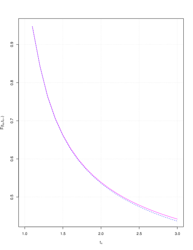
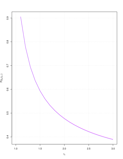
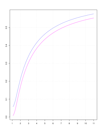
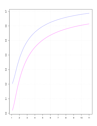
To compare the functions and , we choose the following set of parameters (like those of [20]):, , , and . Figure 1 shows the convergence of the quantized function toward the exact one with , and where is one point, say , on the grid (see equation (21)). Once we fix , depends on both and . Therefore, to show the convergence, we fix
and plot both and with respect to . The number of discretization points is set to and the convergence is achieved by increasing the number of quantization points . Since the fixed quantization point can differ when moving , the corresponding figures can take different shapes but, we have only to make sure that the convergence is achieved when increasing .
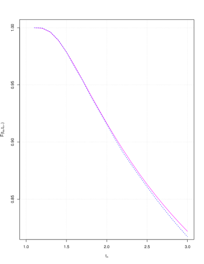
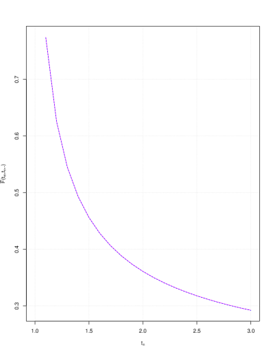
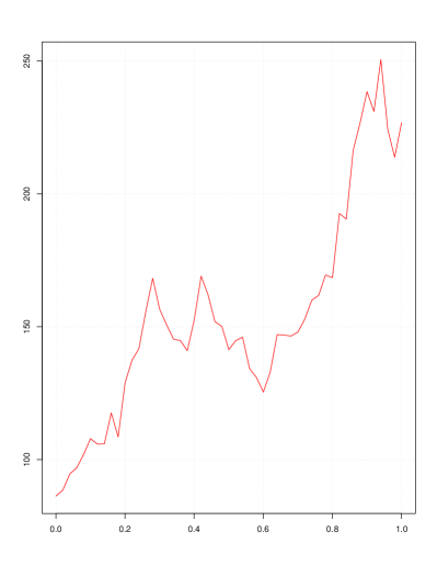
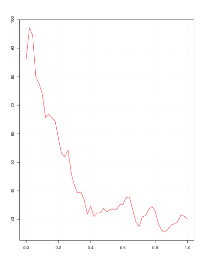
We now proceed to the numerical comparison between the conditional default probabilities and , respectively estimated by (23) and (25), in order to check the statements of Remark 3.1. Setting , and considering the same parameter set as in the previous figure but with , Figure 2 depicts the trajectories of the observation process from to and the associated conditional default probabilities as a function of . First, we notice that equation (6) is fulfilled as given a trajectory of the observation process represented in red, lined up in dots is always above in magenta. Second, the gab between the two quantities is larger for an downward movement of compared to an upward movement for which the firm is less exposed to default. This can be understood by the fact that the more the firm is creditworthy, the less the default information is important and the less the default probability is. Then, the model preserves the memory of all the observed path of the process when computing default probabilities. This path-dependent future of the default probabilities has already been shown in [6] and is known to be very important as it is implicit in reduced-form models for calibration purpose to historical data.
4.2 Application to CDS option pricing
In this section, we briefly recall the concept and valuation of credit default swaps and swaptions before analyzing the quantization procedure applied to such models. This will allow to give a full pricing formula of credit swaps derivatives in a firm value approach using partial information theory and optimal quantization. In addition, the fact that we add the default filtration in the model indicating whether default has already taken place or not is very important in this case as it is pointless to price a default swap post-default.
A credit default swap (CDS) is an agreement between two counterparties to buy or sell protection against the default risk of a third party called reference entity. We set as the default time of the latter. In this case, if the contract is signed at time , started at time with maturity , the protection buyer pays a coupon (or spread) at payments dates as long as the reference entity does not default or until . If the default occurs at time with , the protection seller will make a single payment (that we assume to be a known constant) to the protection buyer. A CDS option (CDSO) or default swaption is an option written on a default swap. From this perspective, it requires to recall the no-arbitrage pricing equation of a CDS. The time- price of a general buyer CDS with unit notional starting at time with maturity , , a spread and loss given default is given by the difference of the conditional risk-neutral expectations of the protection and the premium discounted cashflows:
with the day count fraction between dates and which, in a standard CDS, is around (quarterly payment dates) and is a time- discount factor with maturity and deterministic interest rates . In a reduced-form setup, where , this expression can be developed explicitly thanks to the Key lemma:
| (34) |
where
| (35) |
and is known as the Azéma supermartingale and is the risky duration, i.e. the time- value of the CDS premia paid during the life of the contract when the spread is 1:
The spread which, at time , sets the forward start CDS at 0, called par spread, is given by:
| (36) |
The no-arbitrage price of a call option on such a contract at time becomes
| (37) | |||||
where , with the Dirac delta function centered at .
The random terms inside the expectation (37) mainly the survival processes and are ready to be computed using optimal quantization. To do so, using equations (23) and (25), one only needs to set
| (38) |
Hence the randomness in the expectation (37) is only from the observation process simulated from time to . This means that we should not need a lot of paths when estimating the expectation (37) using Monte Carlo simulation after computing the above mentioned survival processes using optimal quantization. This in turn motivates to fully estimate (37) using a hybrid Monte Carlo-optimal quantization procedure.
A CDS option has little liquidity but, just like usual equity options, is quoted in term of its Black implied volatility which is based on the assumption that the credit spread follows a geometric Brownian motion.111Recall that this does not mean in any way that the market naively believes that credit spreads exhibit log-normal dynamics. Market participants simply rely on the Black-Scholes machinery to convert a price into a quantity that is more intuitive to traders, namely implied volatilities.
The Black formula for payer swaptions at time 0 with maturity is
where
Hence, the CDS option implied volatility can be found by solving the following equation
We now assess the numerical results based on the model’s applications to the pricing of CDS option. The model’s parameter set is the same as before except here we take and is varying. Table 1 shows the estimated values of a European payer CDS option and the corresponding Black’s volatilities with different strikes and different values of . First, we observe that both CDS option prices and the implied volatilities are increasing with the noise volatility, . This can be explained by the fact that, the higher , the noisier the observations are and the higher the default probability. Since measures the degree of transparency of the firm, this will have a positive impact on the prices of the CDS option, hence on the corresponding implied volatilities. In contrast, while the option prices are always decreasing with the strike, this is not the case with the implied volatilities except for and . In the case where , the implied volatility is increasing with respect to the strike. Hence with the help of the parameter , one can observe different levels of skewness.
| (bps) | Payer | Implied vol (%) | ||||
|---|---|---|---|---|---|---|
| % | % | % | % | % | % | |
| 52.9 | 0.004655 | 0.007214 | 0.009276 | 69.44 | 133.84 | 196.80 |
| 66.2 | 0.003739 | 0.006077 | 0.008032 | 73.36 | 124.16 | 173.70 |
| 79.4 | 0.003107 | 0.005298 | 0.007081 | 76.85 | 121.08 | 161.57 |
Notice that in this example, we focus more on the numerical performances of the model and do not address the calibration problem. Hence, we use the model implied term structure given by the time- model survival probability curve as a CDS term structure. Calibration issues of the model to real market data will be investigated in a future work.
5 Conclusion
In this paper, a new structural model for credit risk has been proposed, generalizing earlier works. Our model deals with an incomplete information, where the default state and a noisy observation of the firm valued are accessible to the investor. It is therefore an extension of [6], as the firm-value triggering the default is no longer restricted to be a continuous and invertible function of a Gaussian martingale, but can be any diffusion.
This more general framework benefits however from a limited analytical tractability. Therefore, we propose a numerical method that relies on nonlinear filtering theory associated with recursive quantization. Compared to earlier works such as [5] or [20], our numerical procedure is based on the fast quantization method recently introduced in [17], which avoids the use of Monte Carlo simulations. A rigorous analysis of the global error induced to the estimation of the survival processes is performed. We analyze the shapes of the default probabilities which are characterized by a path-dependent feature keeping the memory of all the path of the observed process. Eventually we quantify the impact of the volatility of the noise impacting the firm-value process on the pricing of CDS options and the corresponding implied volatilities using a hybrid Monte Carlo-optimal quantization method.
In future research, we will first investigate the calibration issues of the model which can be tackled by either using observed prices or CDS quotes. In this case, our model can be easily extended to other works dealing with exact calibration to survival probabilities such as including a specific time-dependent barrier [2] or using time change techniques [13]. Another possible research area is to deal with the price of general default sensitive securities. While we have derived a full quantization scheme to estimate the conditional default probabilities, this was not the case in the pricing of CDS option which required additional Monte Carlo simulations in order to be estimated. To derive a full quantization scheme for the pricing of defaultable claims, a possible route is to exploit the functional quantization method.
References
- [1] F. Black and J. C. Cox. Valuing corporate securities: Some effects of bonds indenture provisions. Journal of Finance, 31:351–367, 1976.
- [2] D. Brigo and M. Tarenghi. Credit default swap calibration and equity swap valuation under counterpaty risk with tractable structural model. In Proceedings of FEA 2004 conference at MIT, 2004.
- [3] D. Brigo and M. Tarenghi. Credit default swap calibration and counterparty risk valuation with a scenario-based first passage model. In Proceedings of the Counterparty Credit Risk 2005 C.R.E.D.I.T. conference, Venice, 22-3 Sptember, 1, 2005.
- [4] J. A. Bucklew and G. L. Wise. Multidimensional asymptotic quantization theory with -th power distribution measures. IEEE Trans. Inform. Theory, 28:239–247, 1982.
- [5] G. Callegaro and A. Sagna. An application to credit risk of optimal quantization methods for nonlinear filtering. The Journal of Computational Finance, 16(4):123–156, 2013.
- [6] D. Coculescu, H. Geman, and M. Jeanblanc. Valuation of default sensitive claims under imperfect information. Finance and Stochastics, 12(2):195–218, 2008.
- [7] D. Duffie and D. Lando. Term structures of credit spreads with incomplete accounting information. Econometrica, 69(3):633–664, 2001.
- [8] R.J. Elliott, M. Jeanblanc, and M. Yor. On models of default risk. Mathematical Finance, 10(2):179–195, 2000.
- [9] R. Frey, L. Rösler, and D. Lu. Corporate security prices in structural credit risk models with incomplete information. Mathematical Finance, 29:84–116, 2019.
- [10] E. Gobet. Schémas d’Euler pour diffusion tuée. Application aux options barrière. PhD thesis, Université Denis Diderot - Paris VII, 1998.
- [11] S. Graf and H. Luschgy. Foundations of Quantization for Probability Distributions. Lect. Notes in Math. 1730. Springer, Berlin., 2000.
- [12] H. Luschgy and G. Pagès. Functional quantization of a class of Brownian diffusions: A constructive approach. Stochastic Processes & Their Applications, 116:310–336, 2006.
- [13] C. Mbaye and F. Vrins. Affine term structure models: a time-changed approach with perfect fit to market curves. Technical report, March 13, 2019. https://arxiv.org/abs/1903.04211.
- [14] R. C. Merton. On the pricing of corporate debt. Journal of Finance, 29:449–470, 1974.
- [15] G. Pagès. A space vector quantization method for numerical integration. J. Computational and Applied Mathematics, 89:1–38, 1998.
- [16] G. Pagès and H. Pham. Optimal quantization methods for nonlinear filtering with discrete time observations. Bernoulli, 11(5):893–932, 2005.
- [17] G. Pagès and A. Sagna. Recursive marginal quantization of the euler scheme of a diffusion process. Applied Mathematical Finance., 22(15):463–498, 2015.
- [18] G. Pagès and A. Sagna. A general weak and strong error analysis of the recursive quantization with an application to jump diffusions. preprint., 2018.
- [19] K. Pötzelberger and L. Wang. Boundary crossing probability for Brownian motion. Journal of applied probability, 38:152–164, 2001.
- [20] C. Profeta and A. Sagna. Conditional hitting time estimation in a nonlinear filtering model by the brownian bridge method. Stochastics: An International Journal of Probability and Stochastic Processes, 2014.
- [21] A. Sagna. Pricing of barrier options by marginal functional quantization method. Monte Carlo Methods and Applications, 17(4):371–398, 2012.
- [22] A. Sellami. Comparative survey on nonlinear filtering methods: the quantization and the particle filtering approaches. Journal of Statistical Computation and Simulation, 78(2):93–113, 2008.
- [23] P. Zador. Asymptotic quantization error of continuous signals and the quantization dimension. IEEE Trans. Inform. Theory, 28:139–149, 1982.