Regularized Linear Inversion with Randomized Singular Value Decomposition

Abstract

In this work, we develop efficient solvers for linear inverse problems based on randomized singular value decomposition (RSVD). This is achieved by combining RSVD with classical regularization methods, e.g., truncated singular value decomposition, Tikhonov regularization, and general Tikhonov regularization with a smoothness penalty. One distinct feature of the proposed approach is that it explicitly preserves the structure of the regularized solution in the sense that it always lies in the range of a certain adjoint operator. We provide error estimates between the approximation and the exact solution under canonical source condition, and interpret the approach in the lens of convex duality. Extensive numerical experiments are provided to illustrate the efficiency and accuracy of the approach.
Keywords:randomized singular value decomposition, Tikhonov regularization, truncated singular value decomposition, error estimate, source condition, low-rank approximation

1 Introduction

This work is devoted to randomized singular value decomposition (RSVD) for the efficient numerical solution of the following linear inverse problem

$$Ax=b,$$ (1.1)

where $A\in\mathbb{R}^{n\times m}$, $x\in\mathbb{R}^{m}$ and $b\in\mathbb{R}^{n}$ denote the data formation mechanism, unknown parameter and measured data, respectively. The data $b$ is generated by $b=b^{\dagger}+e,$ where $b^{\dagger}=Ax^{\dagger}$ is the exact data, and $x^{\dagger}$ and $e$ are the exact solution and noise, respectively. We denote by $\delta=\|e\|$ the noise level.

Due to the ill-posed nature, regularization techniques are often applied to obtain a stable numerical approximation. A large number of regularization methods have been developed. The classical ones include Tikhonov regularization and its variant, truncated singular value decomposition, and iterative regularization techniques, and they are suitable for recovering smooth solutions. More recently, general variational type regularization methods have been proposed to preserve distinct features, e.g., discontinuity, edge and sparsity. This work focuses on recovering a smooth solution by Tikhonov regularization and truncated singular value decomposition, which are still routinely applied in practice. However, with the advent of the ever increasing data volume, their routine application remains challenging, especially in the context of massive data and multi-query, e.g., Bayesian inversion or tuning multiple hyperparameters. Hence, it is still of great interest to develop fast inversion algorithms.

In this work, we develop efficient linear inversion techniques based on RSVD. Over the last decade, a number of RSVD inversion algorithms have been developed and analyzed [10, 11, 20, 31, 26]. RSVD exploits the intrinsic low-rank structure of $A$ for inverse problems to construct an accurate approximation efficiently. Our main contribution lies in providing a unified framework for developing fast regularized inversion techniques based on RSVD, for the following three popular regularization methods: truncated SVD, standard Tikhonov regularization, and Tikhonov regularization with a smooth penalty. The main novelty is that it explicitly preserves a certain range condition of the regularized solution, which is analogous to source condition in regularization theory [5, 13], and admits interpretation in the lens of convex duality. Further, we derive error bounds on the approximation with respect to the true solution $x^{\dagger}$ in Section 4, in the spirit of regularization theory for noisy operators. These results provide guidelines on the low-rank approximation, and differ from existing results [1, 14, 32, 33, 30], where the focus is on relative error estimates with respect to the regularized solution.

Now we situate the work in the literature on RSVD for inverse problems. RSVD has been applied to solving inverse problems efficiently [1, 32, 33, 30]. Xiang and Zou [32] developed RSVD for standard Tikhonov regularization and provided relative error estimates between the approximate and exact Tikhonov minimizer, by adapting the perturbation theory for least-squares problems. In the work [33], the authors proposed two approaches based respectively on transformation to standard form and randomized generalized SVD (RGSVD), and for the latter, RSVD is only performed on the matrix $A$. There was no error estimate in [33]. Wei et al [30] proposed different implementations, and derived some relative error estimates. Boutsidis and Magdon [1] analyzed the relative error for truncated RSVD, and discussed the sample complexity. Jia and Yang [14] presented a different way to perform truncated RSVD via LSQR for general smooth penalty, and provided relative error estimates. See also [16] for an evaluation within magnetic particle imaging. More generally, the idea of randomization has been fruitfully employed to reduce the computational cost associated with regularized inversion in statistics and machine learning, under the name of sketching in either primal or dual spaces [2, 22, 34, 29]. All these works also essentially exploit the low-rank structure, but in a different manner. Our analysis may also be extended to these approaches.

The rest of the paper is organized as follows. In Section 2, we recall preliminaries on RSVD, especially implementation and error bound. Then in Section 3, under one single guiding principle, we develop efficient inversion schemes based on RSVD for three classical regularization methods, and give the error analysis in Section 4. Finally we illustrate the approaches with some numerical results in Section 5. In the appendix, we describe an iterative refinement scheme for (general) Tikhonov regularization. Throughout, we denote by lower and capital letters for vectors and matrices, respectively, by $I$ an identity matrix of an appropriate size, by $\|\cdot\|$ the Euclidean norm for vectors and spectral norm for matrices, and by $(\cdot,\cdot)$ for Euclidean inner product for vectors. The superscript ^∗ denotes the vector/matrix transpose. We use the notation $\mathcal{R}(A)$ and $\mathcal{N}(A)$ to denote the range and kernel of a matrix $A$, and $A_{k}$ and $\tilde{A}_{k}$ denote the optimal and approximate rank-$k$ approximations by SVD and RSVD, respectively. The notation $c$ denotes a generic constant which may change at each occurrence, but is always independent of the condition number of $A$.

2 Preliminaries

Now we recall preliminaries on RSVD and technical lemmas.

2.1 SVD and pseudoinverse

Singular value decomposition (SVD) is one of most powerful tools in numerical linear algebra. For any matrix $A\in\mathbb{R}^{n\times m}$, SVD of $A$ is given by

$$A=U\Sigma V^{*},$$

where $U=[u_{1}\ u_{2}\ \cdots\ u_{n}]\in\mathbb{R}^{n\times n}$ and $V=[v_{1}\ v_{2}\ \cdots\ v_{m}]\in\mathbb{R}^{m\times m}$ are column orthonormal matrices, with the vectors $u_{i}$ and $v_{i}$ being the left and right singular vectors, respectively, and $V^{*}$ denotes the transpose of $V$. The diagonal matrix $\Sigma=\mathrm{diag}(\sigma_{i})\in\mathbb{R}^{n\times m}$ has nonnegative diagonal entries $\sigma_{i}$, known as singular values (SVs), ordered nonincreasingly:

$$\sigma_{1}\geq\sigma_{2}\geq\ldots\geq\sigma_{r}>\sigma_{r+1}=\ldots=\sigma_{\min(m,n)}=0,$$

where $r=\mathrm{rank}(A)$ is the rank of $A$. Let $\sigma_{i}(A)$ be the $i$th SV of $A$. The complexity of the standard Golub-Reinsch algorithm for computing SVD is $4n^{2}m+8m^{2}n+9m^{3}$ (for $n\geq m$) [8, p. 254]. Thus, it is expensive for large-scale problems.

Now we can give the optimal low-rank approximation to $A$. By Eckhardt-Young theorem, the optimal rank-$k$ approximation $A_{k}$ of $A$ (in spectral norm) is given by

$$\|A-U_{k}\Sigma_{k}V^{*}_{k}\|=\sigma_{k+1},$$

where $U_{k}\in\mathbb{R}^{n\times k}$ and $V_{k}\in\mathbb{R}^{m\times k}$ are the submatrix formed by taking the first $k$ columns of the matrices $U$ and $V$, and $\Sigma_{k}=\mathrm{diag}(\sigma_{1},\ldots,\sigma_{k})\in\mathbb{R}^{k\times k}$. The pseudoinverse $A^{\dagger}\in\mathbb{R}^{m\times n}$ of $A\in\mathbb{R}^{n\times m}$ is given by

$$A^{\dagger}=V_{r}\Sigma_{r}^{-1}U_{r}^{*}.$$

We have the following properties of the pseudoinverse of matrix product.

Lemma 2.1.

For any $A\in\mathbb{R}^{m\times n}$, $B\in\mathbb{R}^{n\times l}$, the identity $(AB)^{\dagger}=B^{\dagger}A^{\dagger}$ holds, if one of the following conditions is fulfilled: (i) $A$ has orthonormal columns; (ii) $B$ has orthonormal rows; (iii) $A$ has full column rank and $B$ has full row rank.

The next result gives an estimate on matrix pseudoinverse.

Lemma 2.2.

For symmetric semipositive definite $A,B\in\mathbb{R}^{m\times m}$, there holds

$$\|A^{\dagger}-B^{\dagger}\|\leq\|A^{\dagger}\|\|B^{\dagger}\|\|B-A\|.$$

Proof.

Since $A$ is symmetric semipositive definite, we have $A^{\dagger}=\lim_{\mu\to 0^{+}}(A+\mu I)^{-1}.$ By the identity $C^{-1}-D^{-1}=C^{-1}(D-C)D^{-1}$ for invertible $C,D\in\mathbb{R}^{m\times m}$,

$$A^{\dagger}-B^{\dagger} =\lim_{\mu\to 0^{+}}[(A+\mu I)^{-1}-(B+\mu I)^{-1}]$$

$$=\lim_{\mu\to 0^{+}}[(A+\mu I)^{-1}(B-A)(B+\mu I)^{-1}]=A^{\dagger}(B-A)B^{\dagger}.$$

Now the estimate follows from the matrix spectral norm estimate.∎∎

Remark 2.1.

The estimate for general matrices is weaker than the one in Lemma 2.2: for general $A,B\in\mathbb{R}^{n\times m}$ with $\mathrm{rank}(A)=\mathrm{rank}(B)<\min(m,n)$, there holds [25]

$$\|A^{\dagger}-B^{\dagger}\|\leq\tfrac{1+\sqrt{5}}{2}\|A^{\dagger}\|\|B^{\dagger}\|\|B-A\|.$$

The rank condition is essential, and otherwise, the estimate may not hold.

Last, we recall the stability of SVs ([12, Cor. 7.3.8], [27, Sec. 1.3]).

Lemma 2.3.

For $A,B\in\mathbb{R}^{n\times m}$, there holds

$$|\sigma_{i}(A+B)-\sigma_{i}(A)|\leq\|B\|,\quad i=1,\ldots,\min(m,n).$$

2.2 Randomized SVD

Traditional numerical methods to compute a rank-$k$ SVD, e.g., Lanczos bidiagonalization and Krylov subspace method, are especially powerful for large sparse or structured matrices. However, for many discrete inverse problems, there is no such structure. The prototypical model in inverse problems is a Fredholm integral equation of the first kind, which gives rise to unstructured dense matrices. Over the past decade, randomized algorithms for computing low-rank approximations have gained popularity. Frieze et al [6] developed a Monte Carlo SVD to efficiently compute an approximate low-rank SVD based on non-uniform row and column sampling. Sarlos [23] proposed an approach based on random projection, using properties of random vectors to build a subspace capturing the matrix range. Below we describe briefly the basic idea of RSVD, and refer readers to [11] for an overview and to [10, 20, 26] for an incomplete list of recent works.

RSVD can be viewed as an iterative procedure based on SVDs of a sequence of low-rank matrices to deliver a nearly optimal low-rank SVD. Given a matrix $A\in\mathbb{R}^{n\times m}$ with $n\geq m$, we aim at obtaining a rank-$k$ approximation, with $k\ll\min(m,n)$. Let $\Omega\in\mathbb{R}^{m\times(k+p)}$, with $k+p\leq m$, be a random matrix, with its entries following an i.i.d. Gaussian distribution $N(0,1)$, and the integer $p\geq 0$ is an oversampling parameter (with a default value $p=5$ [11]). Then we form a random matrix $Y$ by

$$Y=(AA^{*})^{q}A\Omega,$$ (2.1)

where the exponent $q\in\mathbb{N}\cup\{0\}$. By SVD of $A$, i.e., $A=U\Sigma V^{*}$, $Y$ is given by

$$Y=U\Sigma^{2q+1}V^{*}\Omega.$$

Thus $\Omega$ is used for probing $\mathcal{R}(A)$, and $\mathcal{R}(Y)$ captures $\mathcal{R}(U_{k})$ well. The accuracy is determined by the decay of $\sigma_{i}$s, and the exponent $q$ can greatly improve the performance when $\sigma_{i}$s decay slowly. Let $Q\in\mathbb{R}^{n\times(k+p)}$ be an orthonormal basis for $\mathcal{R}(Y)$, which can be computed efficiently via QR factorization or skinny SVD. Next we form the (projected) matrix

$$B=Q^{*}A\in\mathbb{R}^{(k+p)\times m}.$$

Last, we compute SVD of $B$

$$B=WSV^{*},$$

with $W\in\mathbb{R}^{(k+p)\times(k+p)}$, $S\in\mathbb{R}^{(k+p)\times(k+p)}$ and $V\in\mathbb{R}^{m\times(k+p)}$. This again can be carried out efficiently by standard SVD, since the size of $B$ is much smaller. With $1:k$ denoting the index set $\{1,\ldots,k\}$, let $\tilde{U}_{k}=QW(1:n,1:k)\in\mathbb{R}^{n\times k}$, $\tilde{\Sigma}_{k}=S(1:k,1:k)\in\mathbb{R}^{k\times k}$ and $\tilde{V}_{k}=V(1:m,1:k)\in\mathbb{R}^{m\times k}$. The triple $(\tilde{U}_{k},\tilde{\Sigma}_{k},\tilde{V}_{k})$ defines a rank-$k$ approximation $\tilde{A}_{k}$:

$$\tilde{A}_{k}=\tilde{U}_{k}\tilde{\Sigma}_{k}\tilde{V}^{*}_{k}.$$

The triple $(\tilde{U}_{k},\tilde{\Sigma}_{k},\tilde{V}_{k})$ is a nearly optimal rank-$k$ approximation to $A$; see Theorem 2.1 below for a precise statement. The approximation is random due to range probing by $\Omega$. By its very construction, we have

$$\tilde{A}_{k}=\tilde{P}_{k}A,$$ (2.2)

where $\tilde{P}_{k}=\tilde{U}_{k}\tilde{U}_{k}^{*}\in\mathbb{R}^{n\times n}$ is the orthogonal projection into $\mathcal{R}(\tilde{U}_{k})$. The procedure for RSVD is given in Algorithm 1. The complexity of Algorithm 1 is about $4(q+1)nmk$, which can be much smaller than that of full SVD if $k\ll\min(m,n)$.

Algorithm 1 RSVD for $A\in\mathbb{R}^{n\times m}$, $n\geq m$.

1:  Input matrix $A\in\mathbb{R}^{n\times m}$, $n\geq m$, and target rank $k$;

2:  Set parameters $p$ (default $p=5$), and $q$ (default $q=0$);

3:  Sample a random matrix $\Omega=(\omega_{ij})\in\mathbb{R}^{m\times(k+p)}$, with $\omega_{ij}\sim N(0,1)$;

4:  Compute the randomized matrix $Y=(AA^{*})^{q}A\Omega$;

5:  Find an orthonormal basis $Q$ of $\mathrm{range}(Y)$ by QR decomposition;

6:  Form the matrix $B=Q^{*}A$;

7:  Compute the SVD of $B=WSV^{*}$;

8:  Return the rank $k$ approximation $(\tilde{U}_{k},\tilde{\Sigma}_{k},\tilde{V}_{k})$, cf. (2.2).

Remark 2.2.

The SV $\sigma_{i}$ can be characterized by [8, Theorem 8.6.1, p. 441]:

$$\sigma_{i}=\max_{\begin{subarray}{c}u\in\mathbb{R}^{n},u\perp\mathrm{span}(\{u_{j}\}_{j=1}^{i-1})\end{subarray}}\frac{\|A^{*}u\|}{\|u\|}.$$

Thus, one may estimate $\sigma_{i}(A)$ directly by $\tilde{\sigma}_{i}(A)=\|A^{*}\tilde{U}(:,i)\|$, and refine the SV estimate, similar to Rayleigh quotient acceleration for computing eigenvalues.

The following error estimates hold for RSVD $(\tilde{U}_{k},\tilde{\Sigma}_{k},\tilde{V}_{k})$ given by Algorithm 1 with $q=0$ [11, Cor. 10.9, p. 275], where the second estimate shows how the parameter $p$ improves the accuracy. The exponent $q$ is in the spirit of a power method, and can significantly improve the accuracy in the absence of spectral gap; see [11, Cor. 10.10, p. 277] for related discussions.

Theorem 2.1.

For $A\in\mathbb{R}^{n\times m}$, $n\geq m$, let $\Omega\in\mathbb{R}^{m\times(k+p)}$ be a standard Gaussian matrix, $k+p\leq m$ and $p\geq 4$, and $Q$ an orthonormal basis for $\mathcal{R}(A\Omega)$. Then with probability at least $1-3p^{-p}$, there holds

$$\|A-QQ^{*}A\|\leq(1+6((k+p)p\log p)^{\frac{1}{2}})\sigma_{k+1}+3\sqrt{k+p}\Big{(}\sum_{j>k}\sigma_{j}^{2}\Big{)}^{\frac{1}{2}},$$

and further with probability at least $1-3e^{-p}$, there holds

$$\|A-QQ^{*}A\|\leq\Big{(}1+16\Big{(}1+\frac{k}{p+1}\Big{)}^{\frac{1}{2}}\Big{)}\sigma_{k+1}+\frac{8(k+p)^{\frac{1}{2}}}{p+1}\Big{(}\sum_{j>k}\sigma_{j}^{2}\Big{)}^{\frac{1}{2}}.$$

The next result is an immediate corollary of Theorem 2.1. Exponentially decaying SVs arise in, e.g., backward heat conduction and elliptic Cauchy problem.

Corollary 2.1.

Suppose that the SVs $\sigma_{i}$ decay exponentially, i.e., $\sigma_{j}=c_{0}c_{1}^{j}$, for some $c_{0}>0$ and $c_{1}\in(0,1)$. Then with probability at least $1-3p^{-p}$, there holds

$$\|A-QQ^{*}A\|\leq\Big{[}1+6((k+p)p\log p)^{\frac{1}{2}}+\frac{3(k+p)^{\frac{1}{2}}}{(1-c_{1}^{2})^{\frac{1}{2}}}\Big{]}\sigma_{k+1},$$

and further with probability at least $1-3e^{-p}$, there holds

$$\|A-QQ^{*}A\|\leq\Big{[}\Big{(}1+16\Big{(}1+\frac{k}{p+1}\Big{)}^{\frac{1}{2}}\Big{)}+\frac{8(k+p)^{\frac{1}{2}}}{(p+1)(1-c_{1}^{2})^{\frac{1}{2}}}\Big{]}\sigma_{k+1}.$$

So far we have assumed that $A$ is tall, i.e., $n\geq m$. For the case $n<m$, one may apply RSVD to $A^{*}$, which gives rise to Algorithm 2.

Algorithm 2 RSVD for $A\in\mathbb{R}^{n\times m},\ n<m$.

1:  Input matrix $A\in\mathbb{R}^{n\times m}$, $n<m$, and target rank $k$;

2:  Set parameters $p$ (default $p=5$), and $q$ (default $q=0$);

3:  Sample a random matrix $\Omega=(\omega_{ij})\in\mathbb{R}^{(k+p)\times n}$, with $\omega_{ij}\sim N(0,1)$;

4:  Compute the randomized matrix $Y=\Omega A(A^{*}A)^{q}$;

5:  Find an orthonormal basis $Q$ of $\mathrm{range}(Y^{*})$ by QR decomposition;

6:  Find the matrix $B=AQ$;

7:  Compute the SVD of $B=USV^{*}$;

8:  Return the rank $k$ approximation $(\tilde{U}_{k},\tilde{\Sigma}_{k},\tilde{V}_{k})$.

The efficiency of RSVD resides crucially on the truly low-rank nature of the problem. The precise spectral decay is generally unknown for many practical inverse problems, although there are known estimates for several model problems, e.g., X-ray transform [18] and magnetic particle imaging [17]. The decay rates generally worsen with the increase of the spatial dimension $d$, at least for integral operators [9], which can potentially hinder the application of RSVD type techniques to high-dimensional problems.

3 Efficient regularized linear inversion with RSVD

Now we develop efficient inversion techniques based on RSVD for problem (1.1) via truncated SVD (TSVD), Tikhonov regularization and Tikhonov regularization with a smoothness penalty [5, 13]. For large-scale inverse problems, this can be expensive, since they either involve full SVD or large dense linear systems. We aim at reducing the cost by exploiting the inherent low-rank structure for inverse problems, and accurately constructing a low-rank approximation by RSVD. This idea has been pursued recently [1, 14, 32, 33, 30]. Our work is along the same line in of research but with a unified framework for deriving all three approaches and interpreting the approach in the lens of convex duality.

The key observation is the range type condition on the approximation $\tilde{x}$:

$$\tilde{x}\in\mathcal{R}(B),$$ (3.1)

with the matrix $B$ is given by

$$B=\left\{\begin{array}[]{ll}A^{*},&\text{truncated SVD, Tikhonov},\\ L^{\dagger}L^{*{\dagger}}A^{*},&\text{general Tikhonov},\end{array}\right.$$

where $L$ is a regularizing matrix, typically chosen to the finite difference approximation of the first- or high-order derivatives [5]. Similar to (3.1), the approximation $\tilde{x}$ is assumed to live in $\mathrm{span}(\{v_{i}\}_{i=1}^{k})$ in [34] for Tikhonov regularization, which is slightly more restrictive than (3.1). An analogous condition on the exact solution $x^{\dagger}$ reads

$$x^{\dagger}=Bw$$ (3.2)

for some $w\in\mathbb{R}^{n}$. In regularization theory [5, 13], (3.2) is known as source condition, and can be viewed as the Lagrange multiplier for the equality constraint $Ax^{\dagger}=b^{\dagger}$, whose existence is generally not ensured for infinite-dimensional problems. It is often employed to bound the error $\|\tilde{x}-x^{\dagger}\|$ of the approximation $\tilde{x}$ in terms of the noise level $\delta$. The construction below explicitly maintains (3.1), thus preserving the structure of the regularized solution $\tilde{x}$. We will interpret the construction by convex analysis. Below we develop three efficient computational schemes based on RSVD.

3.1 Truncated RSVD

Classical truncated SVD (TSVD) stabilizes problem (1.1) by looking for the least-squares solution of

$$\min\|A_{k}x_{k}-b\|,\quad\quad\mbox{with }A_{k}=U_{k}\Sigma_{k}V_{k}^{*}.$$

Then the regularized solution $x_{k}$ is given by

$$x_{k}=A_{k}^{\dagger}b=V_{k}\Sigma_{k}^{-1}U_{k}^{*}b=\sum_{i=1}^{k}\sigma_{i}^{-1}(u_{i},b)v_{i}.$$

The truncated level $k\leq\mathrm{rank}(A)$ plays the role of a regularization parameter, and determines the strength of regularization. TSVD requires computing the (partial) SVD of $A$, which is expensive for large-scale problems. Thus, one can substitute a rank-$k$ RSVD $(\tilde{U}_{k},\tilde{\Sigma}_{k},\tilde{V}_{k})$, leading to truncated RSVD (TRSVD):

$$\hat{x}_{k}=\tilde{V}_{k}\tilde{\Sigma}_{k}^{-1}\tilde{U}_{k}^{*}b.$$

By Lemma 2.3, $\tilde{A}_{k}=\tilde{U}_{k}\tilde{\Sigma}_{k}\tilde{V}_{k}^{*}$ is indeed of rank $k$, if $\|A-\tilde{A}_{k}\|<\sigma_{k}$. This approach was adopted in [1]. Based on RSVD, we propose an approximation $\tilde{x}_{k}$ defined by

$$\tilde{x}_{k}=A^{*}(\tilde{A}_{k}\tilde{A}_{k}^{*})^{{\dagger}}b=A^{*}\sum_{i=1}^{k}\frac{(\tilde{u}_{i},b)}{\tilde{\sigma}_{i}^{2}}\tilde{u}_{i}.$$ (3.3)

By its construction, the range condition (3.1) holds for $\tilde{x}_{k}$. To compute $\tilde{x}_{k}$, one does not need the complete RSVD $(\tilde{U}_{k},\tilde{\Sigma}_{k},\tilde{V}_{k})$ of rank $k$, but only $(\tilde{U}_{k},\tilde{\Sigma}_{k})$, which is advantageous for complexity reduction [8, p. 254]. Given the RSVD $(\tilde{U}_{k},\tilde{\Sigma}_{k})$, computing $\tilde{x}_{k}$ by (3.3) incurs only $O(nk+nm)$ operations.

3.2 Tikhonov regularization

Tikhonov regularization stabilizes (1.1) by minimizing the following functional

$$J_{\alpha}(x)=\tfrac{1}{2}\|Ax-b\|^{2}+\tfrac{\alpha}{2}\|x\|^{2},$$

where $\alpha>0$ is the regularization parameter. The regularized solution $x_{\alpha}$ is given by

$$x_{\alpha}=(A^{*}A+\alpha I)^{-1}A^{*}b=A^{*}(AA^{*}+\alpha I)^{-1}b.$$ (3.4)

The latter identity verifies (3.1). The cost of the step in (3.4) is about $nm^{2}+\frac{m^{3}}{3}$ or $mn^{2}+\frac{n^{3}}{3}$ [8, p. 238], and thus it is expensive for large scale problems. One approach to accelerate the computation is to apply the RSVD approximation $\tilde{A}_{k}=\tilde{U}_{k}\tilde{\Sigma}_{k}\tilde{V}_{k}^{*}$. Then one obtains a regularized approximation [32]

$$\hat{x}_{\alpha}=(\tilde{A}_{k}^{*}\tilde{A}_{k}+\alpha I)^{-1}\tilde{A}_{k}^{*}b.$$ (3.5)

To preserve the range property (3.1), we propose an alternative

$$\tilde{x}_{\alpha}=A^{*}(\tilde{A}_{k}\tilde{A}_{k}^{*}+\alpha I)^{-1}b=A^{*}\sum_{i=1}^{k}\frac{(\tilde{u}_{i},b)}{\tilde{\sigma}_{i}^{2}+\alpha}\tilde{u}_{i}.$$ (3.6)

For $\alpha\to 0^{+}$, $\tilde{x}_{\alpha}$ recovers the TRSVD $\tilde{x}_{k}$ in (3.3). Given RSVD $(\tilde{U}_{k},\tilde{\Sigma}_{k})$, the complexity of computing $\tilde{x}_{\alpha}$ is nearly identical with the TRSVD $\tilde{x}_{k}$.

3.3 General Tikhonov regularization

Now we consider Tikhonov regularization with a general smoothness penalty:

$$J_{\alpha}(x)=\tfrac{1}{2}\|Ax-b\|^{2}+\tfrac{\alpha}{2}\|Lx\|^{2},$$ (3.7)

where $L\in\mathbb{R}^{\ell\times m}$ is a regularizing matrix enforcing smoothness. Typical choices of $L$ include first-order and second-order derivatives. We assume $\mathcal{N}(A)\cap\mathcal{N}(L)=\{0\}$ so that $J_{\alpha}$ has a unique minimizer $x_{\alpha}$. By the identity

$$(A^{*}A+\alpha I)^{-1}A^{*}=A^{*}(AA^{*}+\alpha I)^{-1},$$ (3.8)

if $\mathcal{N}(L)=\{0\}$, the minimizer $x_{\alpha}$ to $J_{\alpha}$ is given by (with $\Gamma=L^{{\dagger}}L^{{\dagger}*}$)

$$x_{\alpha} =(A^{*}A+\alpha L^{*}L)^{-1}(A^{*}y)$$

$$=L^{{\dagger}}((AL^{{\dagger}})^{*}AL^{{\dagger}}+\alpha I)^{-1}(AL^{{\dagger}})^{*}b$$

$$=\Gamma A^{*}(A\Gamma A^{*}+\alpha I)^{-1}b.$$ (3.9)

The $\Gamma$ factor reflects the smoothing property of $\|Lx\|^{2}$. Similar to (3.6), we approximate $B:=AL^{\dagger}$ via RSVD: $\tilde{B}_{k}=U_{k}\Sigma_{k}V_{k}^{*}$, and obtain a regularized solution $\tilde{x}_{\alpha}$ by

$$\tilde{x}_{\alpha}=\Gamma A^{*}(\tilde{B}_{k}\tilde{B}_{k}^{*}+\alpha I)^{-1}b.$$ (3.10)

It differs from [33] in that [33] uses only the RSVD approximation of $A$, thus it does not maintain the range condition (4.2). The first step of Algorithm 1, i.e., $AL^{-1}\Omega$, is to probe $\mathcal{R}(A)$ with colored Gaussian noise with covariance $\Gamma$.

Numerically, it also involves applying $\Gamma$, which can be carried out efficiently if $L$ is structured. If $L$ is rectangular, we have the following decomposition [4, 32]. The $A$-weighted pseudoinverse $L^{\#}$ [4] can be computed efficiently, if $L^{\dagger}$ is easy to compute and the dimensionality of $W$ is small.

Lemma 3.1.

Let $W$ and $Z$ be any matrices satisfying $\mathcal{R}(W)=\mathcal{N}(L)$, $\mathcal{R}(Z)=\mathcal{R}(L)$, $Z^{*}Z=I$, and $L^{\#}=(I-W(AW)^{\dagger}A)L^{\dagger}$. Then the solution $x_{\alpha}$ to (3.7) is given by

$$x_{\alpha}=L^{\#}Z\xi_{\alpha}+W(AW)^{\dagger}b,$$ (3.11)

where the variable $\xi_{\alpha}$ minimizes $\frac{1}{2}\|AL^{\#}Z\xi-b\|^{2}+\frac{\alpha}{2}\|\xi\|^{2}$.

Lemma 3.1 does not necessarily entail an efficient scheme, since it requires an orthonormal basis $Z$ for $\mathcal{R}(L)$. Hence, we restrict our discussion to the case:

$$L\in\mathbb{R}^{\ell\times m}\quad\mbox{ with }\mathrm{rank}(L)=\ell<m.$$ (3.12)

It arises most commonly in practice, e.g., first-order or second-order derivative, and there are efficient ways to perform standard-form reduction. Then we can let $Z=I_{\ell}$. By slightly abusing the notation $\Gamma=L^{\#}L^{\#*}$, by Lemma 3.1, we have

$$x_{\alpha} =L^{\#}((AL^{\#})^{*}AL^{\#}+\alpha I)^{-1}(AL^{\#})^{*}b+W(AW)^{\dagger}b$$

$$=\Gamma A^{*}(A\Gamma A^{*}+\alpha I)^{-1}b+W(AW)^{\dagger}b.$$

The first term is nearly identical with (3.9), with $L^{\#}$ in place of $L^{\dagger}$, and the extra term $W(AW)^{\dagger}b$ belongs to $\mathcal{N}(L)$. Thus, we obtain an approximation $\tilde{x}_{\alpha}$ defined by

$$\tilde{x}_{\alpha}=\Gamma A^{*}(\tilde{B}_{k}\tilde{B}_{k}+\alpha I)^{-1}b+W(AW)^{\dagger}b,$$ (3.13)

where $\tilde{B}_{k}$ is a rank-$k$ RSVD to $B\equiv AL^{\#}$. The matrix $B$ can be implemented implicitly via matrix-vector product to maintain the efficiency.

3.4 Dual interpretation

Now we give an interpretation of (3.10) in the lens of Fenchel duality theory in Banach spaces (see, e.g., [3, Chapter II.4]). Recall that for a functional $F:X\to\overline{\mathbb{R}}:=\mathbb{R}\cup\{\infty\}$ defined on a Banach space $X$, let $F^{*}:X^{*}\to\overline{\mathbb{R}}$ denote the Fenchel conjugate of $F$ given for $x^{*}\in X^{*}$ by

$$F^{*}(x^{*})=\sup_{x\in X}\langle x^{*},x\rangle_{X^{*},X}-F(x).$$

Further, let $\partial F(x):=\{x^{*}\in X^{*}:\langle x^{*},\tilde{x}-x\rangle_{X^{*},X}\leq F(\tilde{x})-F(x)\ \ \forall\tilde{x}\in X\}$ be the subdifferential of the convex functional $F$ at $x$, which coincides with Gâteaux derivative $F^{\prime}(x)$ if it exists. The Fenchel duality theorem states that if $F:X\to\overline{\mathbb{R}}$ and $G:Y\to\overline{\mathbb{R}}$ are proper, convex and lower semicontinuous functionals on the Banach spaces $X$ and $Y$, $\Lambda:X\to Y$ is a continuous linear operator, and there exists an $x_{0}\in W$ such that $F(x_{0})<\infty$, $G(\Lambda x_{0})<\infty$, and $G$ is continuous at $\Lambda x_{0}$, then

$$\inf_{x\in X}F(x)+G(\Lambda x)=\sup_{y^{*}\in Y^{*}}-F^{*}(\Lambda^{*}y^{*})-G^{*}(-y^{*}),$$

Further, the equality is attained at $(\bar{x},\bar{y}^{*})\in X\times Y^{*}$ if and only if

$$\Lambda^{*}\bar{y}^{*}\in\partial F(\bar{x})\quad\mbox{and}\quad-\bar{y}^{*}\in\partial G(\Lambda\bar{x}),$$ (3.14)

hold [3, Remark III.4.2].

The next result indicates that the approach in Sections 3.2-3.3 first applies RSVD to the dual problem to obtain an approximate dual $\tilde{p}_{\alpha}$, and then recovers the optimal primal $\tilde{x}_{\alpha}$ via duality relation (3.14). This connection is in the same spirit of dual random projection [29, 34], and it opens up the avenue to extend RSVD to functionals whose conjugate is simple, e.g., nonsmooth fidelity.

Proposition 3.1.

If $\mathcal{N}(L)=\{0\}$, then $\tilde{x}_{\alpha}$ in (3.10) is equivalent to RSVD for the dual problem.

Proof.

For any symmetric positive semidefinite $Q$, the conjugate functional $F^{*}$ of $F(x)=\frac{\alpha}{2}x^{*}Qx$ is given by $F^{*}(\xi)=-\frac{1}{2\alpha}\xi^{*}Q^{\dagger}\xi$, with its domain being $\mathcal{R}(Q)$. By SVD, we have $(L^{*}L)^{\dagger}=L^{\dagger}L^{{\dagger}*}$, and thus $F^{*}(\xi)=-\frac{1}{2\alpha}\|L^{{\dagger}*}\xi\|^{2}$. Hence, by Fenchel duality theorem, the conjugate $J_{\alpha}^{*}(\xi)$ of $J_{\alpha}(x)$ is given by

$$J^{*}_{\alpha}(\xi):=-\tfrac{1}{2\alpha}\|L^{{\dagger}*}A^{*}\xi\|^{2}-\tfrac{1}{2}\|\xi-b\|^{2}.$$

Further, by (3.14), the optimal primal and dual pair $(x_{\alpha},\xi_{\alpha})$ satisfies

$$\alpha L^{*}Lx_{\alpha}=A^{*}\xi_{\alpha}\quad\mbox{and}\quad\xi_{\alpha}=b-Ax_{\alpha}.$$

Since $\mathcal{N}(L)=\{0\}$, $L^{*}L$ is invertible, and thus $x_{\alpha}=\alpha^{-1}(L^{*}L)^{-1}A^{*}\xi_{\alpha}=\alpha^{-1}\Gamma A^{*}\xi_{\alpha}$. The optimal dual $\xi_{\alpha}$ is given by $\xi_{\alpha}=\alpha(AL^{{\dagger}}L^{*{\dagger}}A^{*}+\alpha I)^{-1}b$. To approximate $\xi_{\alpha}$ by $\tilde{\xi}_{\alpha}$, we employ the RSVD approximation $\tilde{B}_{k}$ to $B=AL^{\dagger}$ and solve

$$\tilde{\xi}_{\alpha}=\arg\max_{\xi\in\mathbb{R}^{n}}\{-\tfrac{1}{2\alpha}\|\tilde{B}_{k}^{*}\xi\|^{2}-\tfrac{1}{2}\|\xi-b\|^{2}\}.$$

We obtain an approximation via the relation $\tilde{x}_{\alpha}=\alpha^{-1}\Gamma A^{*}\tilde{\xi}_{\alpha}$, recovering (3.10).∎∎

Remark 3.1.

For a general regularizing matrix $L$, one can appeal to the decomposition in Lemma 3.1, by applying first the standard transformation and then approximating the regularized part via convex duality.

4 Error analysis

Now we derive error estimates for the approximation $\tilde{x}$ with respect to the true solution $x^{\dagger}$, under sourcewise type conditions. In addition to bounding the error, the estimates provide useful guidelines on constructing the approximation $\tilde{A}_{k}$.

4.1 Truncated RSVD

We derive an error estimate under the source condition (3.2). We use the projection matrices $P_{k}=U_{k}U_{k}^{*}$ and $\tilde{P}_{k}=\tilde{U}_{k}\tilde{U}_{k}^{*}$ frequently below.

Lemma 4.1.

For any $k\leq r$ and $\|A-\tilde{A}_{k}\|\leq\sigma_{k}/2$, there holds $\|A^{*}(\tilde{A}_{k}^{*})^{\dagger}\|\leq 2.$

Proof.

It follows from the decomposition $A=\tilde{P}_{k}A+(I-\tilde{P}_{k})A=\tilde{A}_{k}+(I-\tilde{P}_{k})A$ that

$$\|A^{*}(\tilde{A}_{k}^{*})^{\dagger}\| =\|(\tilde{A}_{k}+(I-\tilde{P}_{k})A)^{*}(\tilde{A}_{k}^{*})^{\dagger}\|\leq\|\tilde{A}_{k}^{*}(\tilde{A}_{k}^{*})^{-1}\|+\|A-\tilde{A}_{k}\|\|\tilde{A}_{k}^{-1}\|$$

$$\leq 1+\tilde{\sigma}_{k}^{-1}\|A-\tilde{A}_{k}\|.$$

Now the condition $\|A-\tilde{A}_{k}\|\leq\sigma_{k}/2$ and Lemma 2.3 imply $\tilde{\sigma}_{k}\geq\sigma_{k}-\|A-\tilde{A}_{k}\|\geq\sigma_{k}/2$, from which the desired estimate follows.∎∎

Now we can state an error estimate for the approximation $\tilde{x}_{k}$.

Theorem 4.1.

If Condition (3.2) holds and $\|A-\tilde{A}_{k}\|\leq\sigma_{k}/2$, then for the estimate $\tilde{x}_{k}$ in (3.3), there holds

$$\|x^{\dagger}-\tilde{x}_{k}\|\leq 4\delta\sigma_{k}^{-1}+8\sigma_{1}\sigma_{k}^{-1}\|A_{k}-\tilde{A}_{k}\|\|w\|+\sigma_{k+1}\|w\|.$$

Proof.

By the decomposition $b=b^{\dagger}+e$, we have (with $P_{k}^{\perp}=I-P_{k}$)

$$\tilde{x}_{k}-x^{\dagger} =A^{*}(\tilde{A}_{k}\tilde{A}_{k}^{*})^{\dagger}b-A^{*}(AA^{*})^{\dagger}b^{\dagger}$$

$$=A^{*}(\tilde{A}_{k}\tilde{A}_{k}^{*})^{{\dagger}}e+A^{*}[(\tilde{A}_{k}\tilde{A}_{k}^{*})^{{\dagger}}-(A_{k}A_{k}^{*})^{{\dagger}}]b^{\dagger}-P_{k}^{\perp}A^{*}(AA^{*})^{{\dagger}}b^{\dagger}.$$

The source condition $x^{\dagger}=A^{*}w$ in (3.2) implies

$$\tilde{x}_{k}-x^{\dagger}=A^{*}(\tilde{A}_{k}\tilde{A}_{k}^{*})^{{\dagger}}e+A^{*}[(\tilde{A}_{k}\tilde{A}_{k}^{*})^{{\dagger}}-(A_{k}A_{k}^{*})^{{\dagger}}]AA^{*}w-P_{k}^{\perp}A^{*}(AA^{*})^{{\dagger}}AA^{*}w.$$

By the triangle inequality, we have

$$\|\tilde{x}_{k}-x^{\dagger}\| \leq\|A^{*}(\tilde{A}_{k}\tilde{A}_{k}^{*})^{{\dagger}}e\|+\|A^{*}[(\tilde{A}_{k}\tilde{A}_{k}^{*})^{{\dagger}}-(A_{k}A_{k}^{*})^{{\dagger}}]AA^{*}w\|$$

$$\quad+\|P_{k}^{\perp}A^{*}(AA^{*})^{{\dagger}}AA^{*}w\|:={\rm I}_{1}+{\rm I}_{2}+{\rm I}_{3}.$$

It suffices to bound the three terms separately. First, for the term ${\rm I}_{1}$, by the identity $(\tilde{A}_{k}\tilde{A}_{k}^{*})^{\dagger}=(\tilde{A}_{k}^{*})^{\dagger}\tilde{A}_{k}^{\dagger}$ and Lemma 4.1, we have

$${\rm I}_{1}\leq\|A^{*}(\tilde{A}_{k}^{*})^{\dagger}\|\|\tilde{A}_{k}^{\dagger}\|\|e\|\leq 2\tilde{\sigma}_{k}^{-1}\delta.$$

Second, for ${\rm I}_{2}$, by Lemmas 4.1 and 2.2 and the identity $(\tilde{A}_{k}\tilde{A}_{k}^{*})^{\dagger}=(\tilde{A}_{k}^{*})^{\dagger}\tilde{A}_{k}^{\dagger}$, we have

$${\rm I}_{2} \leq\|A^{*}[(\tilde{A}_{k}\tilde{A}_{k}^{*})^{{\dagger}}-(A_{k}A_{k}^{*})^{{\dagger}}]AA^{*}\|\|w\|$$

$$\leq\|A^{*}(\tilde{A}_{k}\tilde{A}_{k}^{*})^{\dagger}(\tilde{A}_{k}\tilde{A}_{k}^{*}-A_{k}A_{k}^{*})(A_{k}A_{k}^{*})^{{\dagger}}AA^{*}\|\|w\|$$

$$\leq\|A^{*}(\tilde{A}_{k}^{*})^{\dagger}\|\|\tilde{A}_{k}^{\dagger}\|\|\tilde{A}_{k}\tilde{A}_{k}^{*}-A_{k}A_{k}^{*}\|\|(A_{k}A_{k}^{*})^{\dagger}AA^{*}\|\|w\|$$

$$\leq 4\tilde{\sigma}_{k}^{-1}\|A\|\|A_{k}-\tilde{A}_{k}\|\|w\|,$$

since $\|\tilde{A}_{k}\tilde{A}_{k}^{*}-A_{k}A_{k}^{*}\|\leq\|\tilde{A}_{k}-A_{k}\|(\|\tilde{A}_{k}\|+\|A_{k}^{*}\|)\leq 2\|A\|\|\tilde{A}_{k}-A_{k}\|$ and $\|(A_{k}A_{k}^{*})^{\dagger}AA^{*}\|\leq 1$. By Lemma 2.3, we can bound the term $\|(\tilde{A}_{k}^{*})^{\dagger}\|$ by

$$\|(\tilde{A}_{k}^{*})^{\dagger}\|=\tilde{\sigma}_{k}^{-1}\leq(\sigma_{k}-\|A-\tilde{A}_{k}\|)^{-1}\leq 2\sigma_{k}^{-1}.$$

Last, we can bound the third term ${\rm I}_{3}$ directly by ${\rm I}_{3}\leq\|P_{k}^{\perp}A^{*}\|\|w\|\leq\sigma_{k+1}\|w\|$. Combining these estimates yields the desired assertion.∎∎

Remark 4.1.

The bound in Theorem 4.1 contains three terms: propagation error $\sigma_{k}^{-1}\delta$, approximation error $\sigma_{k+1}\|w\|$, and perturbation error $\sigma_{k}^{-1}\|A\|\|A-\tilde{A}_{k}\|\|w\|$. It is of the worst-case scenario type and can be pessimistic. In particular, the error $\|A^{*}(\tilde{A}_{k}\tilde{A}_{k}^{*})^{-1}e\|$ can be bounded more precisely by

$$\|A^{*}(\tilde{A}_{k}\tilde{A}_{k}^{*})^{{\dagger}}e\|\leq\|A^{*}(\tilde{A}_{k}^{*})^{\dagger}\|\|\tilde{A}_{k}^{\dagger}e\|,$$

and $\|\tilde{A}_{k}^{\dagger}e\|$ can be much smaller than $\tilde{\sigma}_{k}^{-1}\|e\|$, if $e$ concentrates in the high-frequency modes. By balancing the terms, it suffices for $\tilde{A}_{k}$ to have an accuracy $O(\delta)$. This is consistent with the analysis for regularized solutions with perturbed operators.

Remark 4.2.

The condition $\|A-\tilde{A}_{k}\|<\sigma_{k}/2$ in Theorem 4.1 requires a sufficiently accurate low-rank RSVD approximation $(\tilde{U}_{k},\tilde{\Sigma}_{k},\tilde{V}_{k})$ to $A$, i.e., the rank $k$ is sufficiently large. It enables one to define a TRSVD solution $\tilde{x}_{k}$ of truncation level $k$.

Next we give a relative error estimate for $\tilde{x}_{k}$ with respect to the TSVD approximation $x_{k}$. Such an estimate was the focus of a few works [1, 32, 33, 30]. First, we give a bound on $\|\tilde{A}_{k}\tilde{A}_{k}^{*}(A_{k}^{*})^{\dagger}-A_{k}\|$.

Lemma 4.2.

The following error estimate holds

$$\|\tilde{A}_{k}\tilde{A}_{k}^{*}(A_{k}^{*})^{\dagger}-A_{k}\|\leq\left(1+\sigma_{1}\sigma_{k}^{-1}\right)\|A_{k}-\tilde{A}_{k}\|.$$

Proof.

This estimate follows by direct computation:

$$\|\tilde{A}_{k}\tilde{A}_{k}^{*}(A_{k}^{*})^{\dagger}-A_{k}\| =\|[\tilde{A}_{k}\tilde{A}_{k}^{*}-A_{k}A_{k}^{*}](A_{k}^{*})^{\dagger}\|$$

$$\leq\|\tilde{A}_{k}(\tilde{A}_{k}^{*}-A_{k}^{*})(A_{k}^{*})^{\dagger}\|+\|(\tilde{A}_{k}-A_{k})A_{k}^{*}(A_{k}^{*})^{\dagger}\|$$

$$\leq\|\tilde{A}_{k}\|\|\tilde{A}_{k}^{*}-A_{k}^{*}\|\|(A_{k}^{*})^{\dagger}\|+\|\tilde{A}_{k}-A_{k}\|\|A_{k}^{*}(A_{k}^{*})^{\dagger}\|$$

$$\leq(\sigma_{1}\sigma_{k}^{-1}+1)\|\tilde{A}_{k}-A_{k}\|,$$

since $\|\tilde{A}_{k}\|=\|\tilde{P}_{k}A\|\leq\|A\|=\sigma_{1}$. Then the desired assertion follows directly.∎∎

Next we derive a relative error estimate between the approximations $x_{k}$ and $\tilde{x}_{k}$.

Theorem 4.2.

For any $k<r$, and $\|A-\tilde{A}_{k}\|<\sigma_{k}/2$, there holds

$$\frac{\|x_{k}-\tilde{x}_{k}\|}{\|x_{k}\|}\leq 4\Big{(}1+\frac{\sigma_{1}}{\sigma_{k}}\Big{)}\frac{\|A_{k}-\tilde{A}_{k}\|}{\sigma_{k}}.$$

Proof.

We rewrite the TSVD solution $x_{k}$ as

$$x_{k}=A^{*}(A_{k}A_{k}^{*})^{{\dagger}}b=A_{k}^{*}(A_{k}A_{k}^{*})^{\dagger}b.$$ (4.1)

By Lemma 2.3 and the assumption $\|A-\tilde{A}_{k}\|<\sigma_{k}/2$, we have $\tilde{\sigma}_{k}>0.$ Then $x_{k}-\tilde{x}_{k}=A^{*}((A_{k}A_{k}^{*})^{{\dagger}}-(\tilde{A}_{k}\tilde{A}_{k}^{*})^{{\dagger}})b$. By Lemma 2.2,

$$(A_{k}A_{k}^{*})^{\dagger}-(\tilde{A}_{k}\tilde{A}_{k}^{*})^{\dagger}=(\tilde{A}_{k}\tilde{A}_{k}^{*})^{\dagger}(\tilde{A}_{k}\tilde{A}_{k}^{*}-A_{k}A_{k}^{*})(A_{k}A_{k}^{*})^{\dagger}.$$

It follows from the identity $(A_{k}A_{k}^{*})^{\dagger}=(A_{k}^{*})^{\dagger}A_{k}^{\dagger}$ and (4.1) that

$$x_{k}-\tilde{x}_{k} =A^{*}(\tilde{A}_{k}\tilde{A}_{k}^{*})^{\dagger}(\tilde{A}_{k}\tilde{A}_{k}^{*}-A_{k}A_{k}^{*})(A_{k}A_{k}^{*})^{\dagger}b$$

$$=A^{*}(\tilde{A}_{k}\tilde{A}_{k}^{*})^{\dagger}(\tilde{A}_{k}\tilde{A}_{k}^{*}(A_{k}^{*})^{\dagger}-A_{k})A_{k}^{*}(A_{k}A_{k}^{*})^{\dagger}b$$

$$=A^{*}(\tilde{A}_{k}^{*})^{\dagger}\tilde{A}_{k}^{\dagger}(\tilde{A}_{k}\tilde{A}_{k}^{*}(A_{k}^{*})^{\dagger}-A_{k})x_{k}.$$

Thus, we obtain

$$\frac{\|x_{k}-\tilde{x}_{k}\|}{\|x_{k}\|}\leq\|A^{*}(\tilde{A}_{k}^{*})^{\dagger}\|\|\tilde{A}_{k}^{\dagger}\|\|\tilde{A}_{k}\tilde{A}_{k}^{*}(A_{k}^{*})^{\dagger}-A_{k}\|.$$

By Lemma 2.3, we bound the term $\|\tilde{A}_{k}^{\dagger}\|$ by $\|\tilde{A}_{k}^{\dagger}\|\leq 2\sigma_{k}^{-1}.$ Combining the preceding estimates with Lemmas 4.1 and 4.2 completes the proof.∎∎

Remark 4.3.

The relative error is determined by $k$ (and in turn by $\delta$ etc). Due to the presence of the factor $\sigma_{k}^{-2}$, the estimate requires a highly accurate low-rank approximation, i.e., $\|A_{k}-\tilde{A}_{k}\|\ll\sigma_{k}(A)^{-2}$, and hence it is more pessimistic than Theorem 4.1. The estimate is comparable with the perturbation estimate for the TSVD

$$\frac{\|x_{k}-\bar{x}_{k}\|}{\|x_{k}\|}\leq\frac{\sigma_{1}\|A_{k}-\tilde{A}_{k}\|}{\sigma_{k}-\|A_{k}-\tilde{A}_{k}\|}\left(\frac{1}{\sigma_{1}}+\frac{\|Ax_{k}-b\|}{\sigma_{k}\|b\|}\right)+\frac{\|A_{k}-\tilde{A}_{k}\|}{\sigma_{k}}.$$

Modulo the $\alpha$ factor, the estimates in [32, 30] for Tikhonov regularization also depend on $\sigma_{k}^{-2}$ (but can be much milder for a large $\alpha$).

4.2 Tikhonov regularization

The following bounds are useful for deriving error estimate on $\tilde{x}_{\alpha}$ in (3.6).

Lemma 4.3.

The following estimates hold

$$\|(AA^{*}+\alpha I)(\tilde{A}_{k}\tilde{A}_{k}^{*}+\alpha I)^{-1}-I\| \leq 2\alpha^{-1}\|A\|\|A-\tilde{A}_{k}\|,$$

$$\|[(AA^{*}+\alpha I)(\tilde{A}_{k}\tilde{A}_{k}^{*}+\alpha I)^{-1}-I]AA^{*}\| \leq 2\|A\|(2\alpha^{-1}\|A\|\|A-\tilde{A}_{k}\|+1)\|A-\tilde{A}_{k}\|.$$

Proof.

It follows from the identity

$$(AA^{*}+\alpha I)(\tilde{A}_{k}\tilde{A}_{k}^{*}+\alpha I)^{-1}-I=(AA^{*}-\tilde{A}_{k}\tilde{A}_{k}^{*})(\tilde{A}_{k}\tilde{A}_{k}^{*}+\alpha I)^{-1}$$

and the inequality $\|\tilde{A}_{k}\|=\|\tilde{P}_{k}A\|\leq\|A\|$ that

$$\|(AA^{*}+\alpha I)(\tilde{A}_{k}\tilde{A}_{k}^{*}+\alpha I)^{-1}-I\| \leq\alpha^{-1}(\|A\|+\|\tilde{A}_{k}\|)\|A-\tilde{A}_{k}\|$$

$$\leq 2\alpha^{-1}\|A\|\|A-\tilde{A}_{k}\|.$$

Next, by the triangle inequality,

$$\|[(AA^{*}+\alpha I)(\tilde{A}_{k}\tilde{A}_{k}^{*}+\alpha I)^{-1}-I]AA^{*}\|$$

$$\leq \|AA^{*}-\tilde{A}_{k}\tilde{A}_{k}^{*}\|(\|(\tilde{A}_{k}\tilde{A}_{k}^{*}+\alpha I)^{-1}(AA^{*}+\alpha I)\|+\alpha\|(\tilde{A}_{k}\tilde{A}_{k}^{*}+\alpha I)^{-1}\|).$$

This, together with the identity $AA^{*}-\tilde{A}_{k}\tilde{A}_{k}^{*}=A(A^{*}-\tilde{A}_{k}^{*})+(A-\tilde{A}_{k})A_{k}^{*}$ and the first estimate, yields the second estimate, completing the proof of the lemma.∎∎

Now we can give an error estimate on $\tilde{x}_{\alpha}$ in (3.6) under condition (3.2).

Theorem 4.3.

If condition (3.2) holds, then the estimate $\tilde{x}_{\alpha}$ satisfies

$$\|\tilde{x}_{\alpha}-x^{\dagger}\|\leq\alpha^{-\frac{3}{2}}\|A\|\|A-\tilde{A}_{k}\|\big{(}\delta+(2\alpha^{-1}\|A\|\|A-\tilde{A}_{k}\|+1)\alpha\|w\|\big{)}+2^{-1}\alpha^{\frac{1}{2}}\|w\|.$$

Proof.

First, with condition (3.2), $x^{\dagger}$ can be rewritten as

$$x^{\dagger} =(A^{*}A+\alpha I)^{-1}(A^{*}A+\alpha I)x^{\dagger}=(A^{*}A+\alpha I)^{-1}(A^{*}b^{\dagger}+\alpha x^{\dagger})$$

$$=(A^{*}A+\alpha I)^{-1}A^{*}(b^{\dagger}+\alpha w).$$

The identity (3.8) implies $x^{\dagger}=A^{*}(AA^{*}+\alpha I)^{-1}(b^{\dagger}+\alpha w)$. Consequently,

$$\quad\tilde{x}_{\alpha}-x^{\dagger}=A^{*}[(\tilde{A}_{k}\tilde{A}_{k}^{*}+\alpha I)^{-1}b-(AA^{*}+\alpha I)^{-1}(b^{\dagger}+\alpha w)]$$

$$=A^{*}[(\tilde{A}_{k}\tilde{A}_{k}^{*}+\alpha I)^{-1}e+((\tilde{A}_{k}\tilde{A}_{k}^{*}+\alpha I)^{-1}-(AA^{*}+\alpha I)^{-1})b^{\dagger}-\alpha(AA^{*}+\alpha I)^{-1}w].$$

Let $\tilde{I}=(AA^{*}+\alpha I)(\tilde{A}_{k}\tilde{A}_{k}^{*}+\alpha I)^{-1}$. Then by the identity (3.8), there holds

$$(A^{*}A+\alpha I)(\tilde{x}_{\alpha}-x^{\dagger})=A^{*}[\tilde{I}e+(\tilde{I}-I)b^{\dagger}-\alpha w],$$

and taking inner product with $\tilde{x}_{\alpha}-x^{\dagger}$ yields

$$\|A(\tilde{x}_{\alpha}-x^{\dagger})\|^{2}+\alpha\|\tilde{x}_{\alpha}-x^{\dagger}\|^{2}\leq\big{(}\|\tilde{I}e\|+\|(\tilde{I}-I)b^{\dagger}\|+\alpha\|w\|\big{)}\|A(\tilde{x}_{\alpha}-x^{\dagger})\|.$$

By Young’s inequality $ab\leq\frac{1}{4}a^{2}+b^{2}$ for any $a,b\in\mathbb{R}$, we deduce

$$\alpha^{\frac{1}{2}}\|\tilde{x}_{\alpha}-x^{\dagger}\|\leq 2^{-1}(\|\tilde{I}e\|+\|(\tilde{I}-I)b^{\dagger}\|+\alpha\|w\|).$$

By Lemma 4.3 and the identity $b^{\dagger}=AA^{*}w$, we have

$$\|\tilde{I}e\| \leq 2\alpha^{-1}\|A\|\|A-\tilde{A}_{k}\|\delta,$$

$$\|(\tilde{I}-I)b^{\dagger}\| =\|(\tilde{I}-I)AA^{*}w\|$$

$$\leq 2\|A\|(2\alpha^{-1}\|A\|\|A-\tilde{A}_{k}\|+1)\|A-\tilde{A}_{k}\|\|w\|.$$

Combining the preceding estimates yield the desired assertion.∎∎

Remark 4.4.

To maintain the error $\|\tilde{x}_{\alpha}-x^{\dagger}\|$, the accuracy of $\tilde{A}_{k}$ should be of $O(\delta)$, and $\alpha$ should be of $O(\delta)$, which gives an overall accuracy $O(\delta^{1/2})$. The tolerance on $\|A-\tilde{A}_{k}\|$ can be relaxed for high noise levels. It is consistent with existing theory for Tikhonov regularization with noisy operators [19, 21, 28].

Remark 4.5.

The following relative error estimate was shown [32, Theorem 1]:

$$\frac{\|x_{\alpha}-\hat{x}_{\alpha}\|}{\|x_{\alpha}\|}\leq c(2\sec\theta\kappa+\tan\theta\kappa^{2})\sigma_{k+1}+O(\sigma_{k+1}^{2}),$$

with $\theta=\sin^{-1}\frac{(\|b-Ax_{\alpha}\|^{2}+\alpha\|x_{\alpha}\|^{2})^{\frac{1}{2}}}{\|b\|}$ and $\kappa=(\sigma_{1}^{2}+\alpha)(\frac{\alpha^{\frac{1}{2}}}{\sigma_{n}^{2}+\alpha}+\max_{1\leq i\leq n}\frac{\sigma_{i}}{\sigma_{i}^{2}+\alpha})$. $\kappa$ is a variant of condition number. Thus, $\tilde{A}_{k}$ should approximate accurately $A$ in order not to spoil the accuracy, and the estimate can be pessimistic for small $\alpha$ for which the estimate tends to blow up.

4.3 General Tikhonov regularization

Last, we give an error estimate for $\tilde{x}_{\alpha}$ defined in (3.10) under the following condition

$$x^{\dagger}=\Gamma A^{*}w,$$ (4.2)

where $\mathcal{N}(L)=\{0\}$, and $\Gamma=L^{\dagger}L^{*{\dagger}}$. Also recall that $B=A\Gamma^{\dagger}$.

Theorem 4.4.

If Condition (4.2) holds, then the regularized solution $\tilde{x}_{\alpha}$ in (3.10) satisfies

$$\|L(x^{\dagger}-\tilde{x}_{\alpha})\|\leq\alpha^{-\frac{3}{2}}\|B\|\|B-\tilde{B}_{k}\|\big{(}\delta+(2\alpha^{-1}\|B\|\|B-\tilde{B}_{k}\|+1)\alpha\|w\|\big{)}+2^{-1}\alpha^{\frac{1}{2}}\|w\|.$$

Proof.

First, by the source condition (4.2), we rewrite $x^{\dagger}$ as

$$x^{\dagger} =(A^{*}A+\alpha L^{*}L)^{-1}(A^{*}A+\alpha L^{*}L)x^{\dagger}$$

$$=(A^{*}A+\alpha L^{*}L)^{-1}(A^{*}b^{\dagger}+\alpha A^{*}w).$$

Now with the identity $(A^{*}A+\alpha L^{*}L)^{-1}A^{*}=\Gamma A^{*}(A\Gamma A^{*}+\alpha I)^{-1},$ we have

$$x^{\dagger}=\Gamma A^{*}(A\Gamma A^{*}+\alpha I)^{-1}(b^{\dagger}+\alpha w).$$

Thus, upon recalling $B=AL^{\dagger}$, we have

$$\quad\tilde{x}_{\alpha}-x^{\dagger}=\Gamma A^{*}[(\tilde{B}_{k}\tilde{B}_{k}^{*}+\alpha I)^{-1}b-(BB^{*}+\alpha I)^{-1}(b^{\dagger}+\alpha w)]$$

$$=\Gamma A^{*}[(\tilde{B}_{k}\tilde{B}_{k}^{*}+\alpha I)^{-1}e+((\tilde{B}_{k}\tilde{B}_{k}^{*}+\alpha I)^{-1}-(BB^{*}+\alpha I)^{-1})b^{\dagger}-\alpha(BB^{*}+\alpha I)^{-1}w].$$

It follows from the identity

$$(A^{*}A+\alpha L^{*}L)\Gamma A^{*}=(A^{*}A+\alpha L^{*}L)L^{{\dagger}}L^{{\dagger}*}A^{*}=A^{*}(BB^{*}+\alpha I),$$

that

$$(A^{*}A+\alpha L^{*}L)(\tilde{x}_{\alpha}-x^{\dagger})=A^{*}[\tilde{I}e+(\tilde{I}-I)b^{\dagger}-\alpha w],$$

with $\tilde{I}=(BB^{*}+\alpha I)(\tilde{B}_{k}\tilde{B}_{k}^{*}+\alpha I)^{-1}$. Taking inner product with $x_{\alpha}-x^{\dagger}$ and applying Cauchy-Schwarz inequality yield

$$\|A(\tilde{x}_{\alpha}-x^{\dagger})\|^{2}+\alpha\|L(\tilde{x}_{\alpha}-x^{\dagger})\|^{2}\leq(\|\tilde{I}e\|+\|(\tilde{I}-I)b^{\dagger}\|+\|\alpha w\|)\|A(\tilde{x}_{\alpha}-x^{\dagger})\|,$$

Young’s inequality implies $\alpha^{\frac{1}{2}}\|L(\tilde{x}_{\alpha}-x^{\dagger})\|\leq 2^{-1}(\|\tilde{I}e\|+\|(\tilde{I}-I)b^{\dagger}\|+\alpha\|w\|)$. The identity $b^{\dagger}=Ax^{\dagger}=AL^{{\dagger}}L^{{\dagger}*}A^{*}w=BB^{*}w$ from (4.2) and Lemma 4.3 complete the proof.∎∎

5 Numerical experiments and discussions

Now we present numerical experiments to illustrate our approach. The noisy data $b$ is generated from the exact data $b^{\dagger}$ as follows

$$b_{i}=b_{i}^{\dagger}+\delta\max_{j}(|b_{j}^{\dagger}|)\xi_{i},\quad i=1,\ldots,n,$$

where $\delta$ is the relative noise level, and the random variables $\xi_{i}$s follow the standard Gaussian distribution. All the computations were carried out on a personal laptop with 2.50 GHz CPU and 8.00G RAM by MATLAB 2015b. When implementing Algorithm 1, the default choices $p=5$ and $q=0$ are adopted. Since the TSVD and Tikhonov solutions are close for suitably chosen regularization parameters, we present only results for Tikhonov regularization (and the general case with $L$ given by the first-order difference, which has a one-dimensional kernel $\mathcal{N}(L)$).

Throughout, the regularization parameter $\alpha$ is determined by uniformly sampling an interval on a logarithmic scale, and then taking the value attaining the smallest reconstruction error, where approximate Tikhonov minimizers are found by either (3.6) or (3.13) with a large $k$ ($k=100$ in all the experiments).

5.1 One-dimensional benchmark inverse problems

First, we illustrate the efficiency and accuracy of proposed approach, and compare it with existing approaches [32, 33]. We consider seven examples (i.e., deriv2, heat, phillips, baart, foxgood, gravity and shaw), taken from the popular public-domain MATLAB package regutools (available from http://www.imm.dtu.dk/~pcha/Regutools/, last accessed on January 8, 2019), which have been used in existing studies (see, e.g., [30, 32, 33]). They are Fredholm integral equations of the first kind, with the first three examples being mildly ill-posed (i.e., $\sigma_{i}$s decay algebraically) and the rest severely ill-posed (i.e., $\sigma_{i}$s decay exponentially). Unless otherwise stated, the examples are discretized with a dimension $n=m=5000$. The resulting matrices are dense and unstructured. The rank $k$ of $\tilde{A}_{k}$ is fixed at $k=20$, which is sufficient to for all examples.

The numerical results by standard Tikhonov regularization and two randomized variants, i.e., (3.5) and (3.6), for the examples are presented in Table 1. The accuracy of the approximations, i.e., the Tikhonov solution $x_{\alpha}$, and two randomized approximations $\hat{x}_{\alpha}$ (cf. (3.5), proposed in [32]) and $\tilde{x}_{\alpha}$ (cf. (3.6), the proposed in this work), is measured in two different ways:

$$\tilde{e}_{xz} =\|\hat{x}_{\alpha}-x_{\alpha}\|,\quad\tilde{e}_{ij}=\|\tilde{x}_{\alpha}-x_{\alpha}\|,$$

$$e =\|x_{\alpha}-x^{\dagger}\|,\quad e_{xz}=\|\hat{x}_{\alpha}-x^{\dagger}\|,\quad e_{ij}=\|\tilde{x}_{\alpha}-x^{\dagger}\|,$$

where the methods are indicated by the subscripts. That is, $\tilde{e}_{xz}$ and $\tilde{e}_{ij}$ measure the accuracy with respect to the Tikhonov solution $x_{\alpha}$, and $e$, $e_{xz}$ and $e_{ij}$ measure the accuracy with respect to the exact one $x^{\dagger}$.

The following observations can be drawn from Table 1. For all examples, the three approximations $x_{\alpha}$, $\tilde{x}_{\alpha}$ and $\hat{x}_{\alpha}$ have comparable accuracy relative to the exact solution $x^{\dagger}$, and the errors $e_{ij}$ and $e_{xz}$ are fairly close to the error $e$ of the Tikhonov solution $x_{\alpha}$. Thus, RSVD can maintain the reconstruction accuracy. For heat, despite the apparent large magnitude of the errors $\tilde{e}_{xz}$ and $\tilde{e}_{ij}$, the errors $e_{xz}$ and $e_{ij}$ are not much worse than $e$. A close inspection shows that the difference of the reconstructions are mostly in the tail part, which requires more modes for a full resolution. The computing time (in seconds) for obtaining $x_{\alpha}$ and $\tilde{x}_{\alpha}$ and $\hat{x}_{\alpha}$ is about $6.60$, $0.220$ and $0.220$, where for the latter two, it includes also the time for computing RSVD. Thus, for all the examples, with a rank $k=20$, RSVD can accelerate standard Tikhonov regularization by a factor of 30, while maintaining the accuracy, and the proposed approach is competitive with the one in [32]. Note that the choice $k=20$ can be greatly reduced for severely ill-posed problems; see Section 5.2 below for discussions.

Table 1: Numerical results by standard Tikhonov regularization at two noise levels.

example	$\delta$	$\tilde{e}_{xz}$	$\tilde{e}_{ij}$	$e$	$e_{xz}$	$e_{ij}$
baart	$1\%$	1.14e-9	1.14e-9	1.68e-1	1.68e-1	1.68e-1
	$5\%$	5.51e-11	6.32e-11	2.11e-1	2.11e-1	2.11e-1
deriv2	$1\%$	2.19e-2	2.41e-2	1.18e-1	1.20e-1	1.13e-1
	$5\%$	1.88e-2	2.38e-2	1.59e-1	1.60e-1	1.62e-1
foxgood	$1\%$	2.78e-7	2.79e-7	4.93e-1	4.93e-1	4.93e-1
	$5\%$	1.91e-7	1.96e-7	1.18e0	1.18e0	1.18e0
gravity	$1\%$	1.38e-4	1.41e-4	7.86e-1	7.86e-1	7.86e-1
	$5\%$	1.83e-4	1.84e-4	2.63e0	2.63e0	2.63e0
heat	$1\%$	1.33e0	1.13e0	9.56e-1	1.67e0	1.50e0
	$5\%$	9.41e-1	9.45e-1	2.02e0	1.70e0	1.99e0
phillips	$1\%$	5.53e-3	4.09e-3	6.28e-2	6.19e-2	6.24e-2
	$5\%$	6.89e-3	7.53e-3	9.57e-2	9.53e-2	9.79e-2
shaw	$1\%$	3.51e-9	3.49e-9	4.36e0	4.36e0	4.36e0
	$5\%$	1.34e-9	1.37e-9	8.23e0	8.23e0	8.23e0

The preceding observations remain largely valid for general Tikhonov regularization; see Table 2. Since the construction of the approximation $\hat{x}_{\alpha}$ does not retain the structure of the regularized solution $x_{\alpha}$, the error $\tilde{e}_{xz}$ can potentially be much larger than $\tilde{e}_{ij}$, which can indeed be observed. The errors $e$, $e_{xz}$ and $e_{ij}$ are mostly comparable, except for deriv2. For deriv2, the approximation $\hat{x}_{\alpha}$ suffers from grave errors, since the projection of $L$ into $\mathcal{R}(Q)$ is very inaccurate for preserving $L$. It is expected that the loss occurs whenever general Tikhonov penalty is much more effective than the standard one. This shows the importance of structure preservation. Note that, for a general $L$, $\tilde{x}_{\alpha}$ takes only about 1.5 times the computing time of $\hat{x}_{\alpha}$. This cost can be further reduced since $L$ is highly structured and admits fast inversion. Thus preserving the range structure of $x_{\alpha}$ in (3.1) does not incur much overhead.

Table 2: Numerical results by general Tikhonov regularization (with the first-order derivative penalty) for the examples at two noise levels.

example	$\delta$	$\tilde{e}_{xz}$	$\tilde{e}_{ij}$	$e$	$e_{xz}$	$e_{ij}$
baart	$1\%$	3.35e-10	2.87e-10	1.43e-1	1.43e-1	1.43e-1
	$5\%$	3.11e-10	8.24e-12	1.48e-1	1.48e-1	1.48e-1
deriv2	$1\%$	1.36e-1	4.51e-4	1.79e-2	1.48e-1	1.78e-2
	$5\%$	1.57e-1	3.85e-4	2.40e-2	1.77e-1	2.40e-2
foxgood	$1\%$	4.84e-2	2.26e-8	9.98e-1	1.02e0	9.98e-1
	$5\%$	1.90e-2	1.51e-9	2.27e0	2.28e0	2.27e0
gravity	$1\%$	3.92e-2	2.33e-5	1.39e0	1.41e0	1.39e0
	$5\%$	1.96e-2	9.47e-6	3.10e0	3.10e0	3.10e0
heat	$1\%$	5.54e-1	8.74e-1	8.95e-1	1.06e0	1.32e0
	$5\%$	8.90e-1	1.01e0	1.87e0	1.76e0	1.99e0
phillips	$1\%$	3.25e-3	3.98e-4	6.14e-2	6.06e-2	6.14e-2
	$5\%$	5.64e-3	5.82e-4	8.37e-2	8.18e-2	8.34e-2
shaw	$1\%$	3.79e-4	3.70e-8	3.32e0	3.32e0	3.32e0
	$5\%$	9.73e-4	2.17e-8	9.23e0	9.23e0	9.23e0

Last, we present some results on the computing time for deriv2 versus the problem dimension, and at two truncation levels for RSVD, i.e., $k=20$ and $k=30$. The numerical results are given in Fig. 1. The cubic scaling of the standard approach and quadratic scaling of the approach based on RSVD are clearly observed, confirming the complexity analysis in Sections 2 and 3. In both (3.6) and (3.13), computing RSVD represents the dominant part of the overall computational efforts, and thus the increase of the rank $k$ from 20 to 30 adds very little overheads (compare the dashed and solid curves in Fig. 1). Further, for Tikhonov regularization, the two randomized variants are equally efficient, and for the general one, the proposed approach is slightly more expensive due to its direct use of $L$ in constructing the approximation $\tilde{B}_{k}$ to $B:=AL^{\#}$. Although not presented, we note that the results for other examples are very similar.

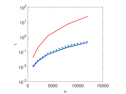
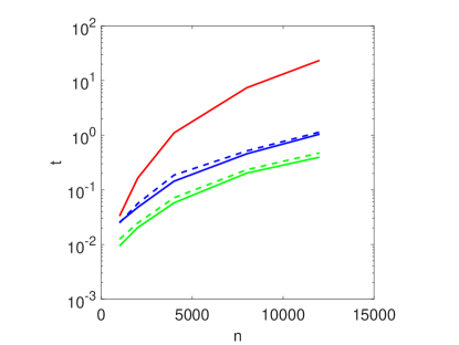
(a) standard Tikhonov	(b) general Tikhonov

Figure 1: The computing time $t$ (in seconds) for the example deriv2 at different dimension $n$ ($m=n$). The red, green and blue curves refer to Tikhonov regularization, existing approach [32, 33] and the new approach, respectively, and the sold and dashed curves denote $k=20$ and $k=30$, respectively.

5.2 Convergence of the algorithm

There are several factors influencing the quality of $\tilde{x}_{\alpha}$ the regularization parameter $\alpha$, the noise level $\delta$ and the rank $k$ of the RSVD approximation. The optimal truncation level $k$ should depend on both $\alpha$ and $\delta$. This part presents a study with deriv2 and shaw, which are mildly and severely ill-posed, respectively.

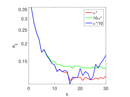
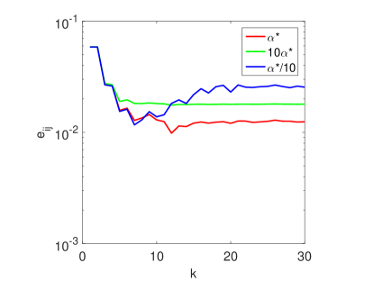
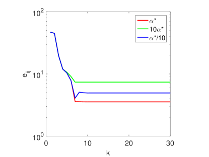
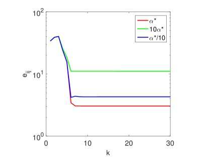
(a) standard Tikhonov	(b) general Tikhonov

Figure 2: The convergence of the error $e_{ij}$ with respect to the rank $k$ for deriv2 (top) and shaw (bottom) with $\delta=1\%$ and different regularization parameters.

First, we examine the influence of $\alpha$ on the optimal $k$. The numerical results for three different levels of regularization are given in Fig. 2. In the figure, the notation $\alpha^{*}$ refers to the value attaining the the smallest error for Tikhonov solution $x_{\alpha}$, and thus $10\alpha^{*}$ and $\alpha^{*}/10$ represent respectively over- and under-regularization. The optimal $k$ value decreases with the increase of $\alpha$ when $\alpha\gg\alpha^{*}$. This may be explained by the fact that a too large $\alpha$ causes large approximation error and thus can tolerate large errors in the approximation $\tilde{A}_{k}$ (for a small $k$). The dependence can be sensitive for mildly ill-posed problems, and also on the penalty. The penalty influences the singular value spectra in the RSVD approximation implicitly by preconditioning: since $L$ is a discrete differential operator, the (weighted) pseudoinverse $L^{\#}$ (or $L^{\dagger}$) is a smoothing operator, and thus the singular values of $B=AL^{\#}$ decay faster than that of $A$. In all cases, the error $e_{ij}$ is nearly monotonically decreasing in $k$ (and finally levels off at $e$, as expected). In the under-regularized regime (i.e., $\alpha\ll\alpha^{*}$), the behavior is slightly different: the error $e_{ij}$ first decreases, and then increases before eventually leveling off at $e$. This is attributed to the fact that proper low-rank truncation of $A$ induces extra regularization, in a manner similar to TSVD in Section 3.1. Thus, an approximation that is only close to $x_{\alpha}$ (see e.g., [1, 32, 33, 30]) is not necessarily close to $x^{\dagger}$, when $\alpha$ is not chosen properly.

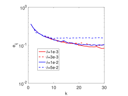
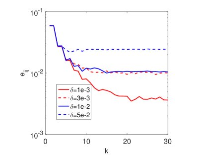
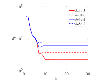
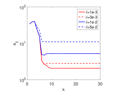
(a) standard Tikhonov	(b) general Tikhonov

Figure 3: The convergence of the error $e_{ij}$ with respect to the rank $k$ for deriv2 (top) and shaw (bottom) at different noise levels.

Next we examine the influence of the noise level $\delta$; see Fig. 3. With the optimal choice of $\alpha$, the optimal $k$ increases as $\delta$ decreases, which is especially pronounced for mildly ill-posed problems. Thus, RSVD is especially efficient for the following two cases: (a) highly noisy data (b) severely ill-posed problem. These observations agree well with Theorem 4.3: a low-rank approximation $\tilde{A}_{k}$ whose accuracy is commensurate with $\delta$ is sufficient, and in either case, a small rank is sufficient for obtaining an acceptable approximation. For a fixed $k$, the error $e_{ij}$ almost increases monotonically with the noise level $\delta$.

These empirical observations naturally motivate developing an adaptive strategy for choosing the rank $k$ on the fly so as to effect the optimal complexity. This requires a careful analysis of the balance between $k$, $\delta$, $\alpha$, and suitable a posteriori estimators. We leave this interesting topic to a future work.

5.3 Electrical impedance tomography

Last, we illustrate the approach on 2D electrical impedance tomography (EIT), a diffusive imaging modality of recovering the electrical conductivity from boundary voltage measurement. This is one canonical nonlinear inverse problem. We consider the problem on a unit circle with sixteen electrodes uniformly placed on the boundary, and adopt the complete electrode model [24] as the forward model. It is discretized by the standard Galerkin FEM with conforming piecewise linear basis functions, on a quasi-uniform finite element mesh with $2129$ nodes. For the inversion step, we employ ten sinusoidal input currents, unit contact impedance and measure the voltage data (corrupted by $\delta=0.1\%$ noise). The reconstructions are obtained with an $H^{1}(\Omega)$-seminorm penalty. We refer to [7, 15] for details on numerical implementation. We test the RSVD algorithm with the linearized model. It can be implemented efficiently without explicitly computing the linearized map. More precisely, let $F$ be the (nonlinear) forward operator, and $\sigma_{0}$ be the background (fixed at $1$). Then the random probing of the range $\mathcal{R}(F^{\prime}(\sigma_{0}))$ of the linearized forward operator $F^{\prime}(\sigma_{0})$ (cf. Step 4 of Algorithm 1) can be approximated by

$$F^{\prime}(\sigma_{0})\omega_{i}\approx F(\sigma_{0}+\omega_{i})-F(\sigma_{0}),\quad i=1,\ldots k+p,$$

and it can be made very accurate by choosing a small variance for the random vector $\omega_{i}$. Step 6 of Algorithm 1 can be done efficiently via the adjoint technique.

The numerical results are presented in Fig. 4, where linearization refers to the reconstruction by linearizing the nonlinear forward model at the background $\sigma_{0}$. This is one of the most classical reconstruction methods in EIT imaging. The rank $k$ is taken to be $k=30$ for $\tilde{x}_{\alpha}$, which is sufficient given the severe ill-posed nature of the EIT inverse problem. Visually, the RSVD reconstruction is indistinguishable from the conventional approach. Note that contrast loss is often observed for EIT reconstructions obtained by a smoothness penalty. The computing time (in seconds) for RSVD is less than 8, whereas that for the conventional method is about 60. Hence, RSVD can greatly accelerate EIT imaging.

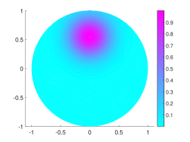
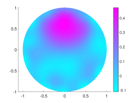
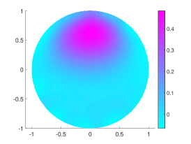
exact	linearization	RSVD

Figure 4: Numerical reconstructions for EIT with $0.1\%$ noise.

6 Conclusion

In this work, we have provided a unified framework for developing efficient linear inversion techniques via RSVD and classical regularization methods, building on a certain range condition on the regularized solution. The construction is illustrated on three popular linear inversion methods for finding smooth solutions, i.e., truncated singular value decomposition, Tikhonov regularization and general Tikhonov regularization with a smoothness penalty. We have provided a novel interpretation of the approach via convex duality, i.e., it first approximates the dual variable via randomized SVD and then recovers the primal variable via duality relation. Further, we gave rigorous error bounds on the approximation under the canonical sourcewise representation, which provide useful guidelines for constructing a low-rank approximation. We have presented extensive numerical experiments, including nonlinear tomography, to illustrate the efficiency and accuracy of the approach, and demonstrated its competitiveness with existing methods.

Algorithm 3 Iterative refinement of RSVD-Tikhonov solution.

1:  Give $A$, $b$ and $J$, and initialize $(x^{0},p^{0})=(0,0)$.

2:  Compute RSVD $(\tilde{U}_{k},\tilde{\Sigma}_{k},\tilde{V}_{k})$ to $AL^{\dagger}$ by Algorithm 1.

3:  for $j=1,\ldots,J$ do

4:     Compute the auxiliary variable $z^{j}$ by (.2).

5:     Update the dual variable $p^{j+1}$ by (.3).

6:     Update the primal variable $x^{j+1}$ by (.4).

7:     Check the stopping criterion.

8:  end for

9:  Output $x^{J}$ as an approximation to $x_{\alpha}$.

Appendix A: Iterative refinement

Proposition 3.1 enables iteratively refining the inverse solution when RSVD is not sufficiently accurate. This idea was proposed in [29, 34] for standard Tikhonov regularization, and we describe the procedure in a slightly more general context. Suppose $\mathcal{N}(L)=\{0\}$. Given a current iterate $x^{j}$, we define a functional $J_{\alpha}^{j}(\delta x)$ for the increment $\delta x$ by

$$J_{\alpha}^{j}(\delta x):=\|A(\delta x+x^{j})-b\|^{2}+\alpha\|L(\delta x+x^{j})\|^{2}.$$

Thus the optimal correction $\delta x_{\alpha}$ satisfies

$$(A^{*}A+\alpha L^{*}L)\delta x_{\alpha}=A^{*}(b-Ax^{j})-\alpha L^{*}Lx^{j},$$

i.e.,

$$(B^{*}B+\alpha I)L\delta x_{\alpha}=B^{*}(b-Ax^{j})-\alpha Lx^{j},$$ (.1)

with $B=AL^{\dagger}$. However, its direct solution is expensive. We employ RSVD for a low-dimensional space $\tilde{V}_{k}$ (corresponding to $B$), parameterize the increment $L\delta x$ by $L\delta x=\tilde{V}_{k}^{*}z$ and update $z$ only. That is, we minimize the following functional in $z$

$$J_{\alpha}^{j}(z):=\|A(L^{{\dagger}}\tilde{V}_{k}^{*}z+x^{j})-b\|^{2}+\alpha\|z+\tilde{V}_{k}Lx^{j}\|^{2}.$$

Since $k\ll m$, the problem can be solved efficiently. More precisely, given the current estimate $x^{j}$, the optimal $z$ solves

$$(\tilde{V}_{k}B^{*}B\tilde{V}_{k}^{*}+\alpha I)z=\tilde{V}_{k}B^{*}(b-Ax^{j})-\alpha\tilde{V}_{k}Lx^{j}.$$ (.2)

It is the Galerkin projection of (.1) for $\delta x_{\alpha}$ onto the subspace $\tilde{V}_{k}$. Then we update the dual $\xi$ and the primal $x$ by the duality relation in Section Appendix A: Iterative refinement:

$$\xi^{j+1} =b-Ax^{j}-B\tilde{V}_{k}^{*}z^{j},$$ (.3)

$$x^{j+1} =\alpha^{-1}\Gamma A^{*}\xi^{j+1}.$$ (.4)

Summarizing the steps gives Algorithm 3. Note that the duality relation (3.14) enables $A$ and $A^{*}$ to enter into the play, thereby allowing progressively improving the accuracy. The main extra cost lies in matrix-vector products by $A$ and $A^{*}$.

The iterative refinement is a linear fixed-point iteration, with the solution $x_{\alpha}$ being a fixed point and the iteration matrix being independent of the iterate. Hence, if the first iteration is contractive, i.e., $\|x^{1}-x_{\alpha}\|\leq c\|x^{0}-x_{\alpha}\|$, for some $c\in(0,1)$, then Algorithm 3 converges linearly to $x_{\alpha}$. It can be satisfied if the RSVD approximation $(\tilde{U}_{k},\tilde{\Sigma}_{k},\tilde{V}_{k})$ is reasonably accurate to $B$.

References

- [1] C. Boutsidis and M. Magdon-Ismail, Faster SVD-truncated regularized least-squares, in 2014 IEEE International Symposium on Information Theory, 2014, pp. 1321–1325.
- [2] S. Chen, Y. Liu, M. R. Lyu, I. King, and S. Zhang, Fast relative-error approximation algorithm for ridge regression, in Proc. 31st Conf. Uncertainty in Artificial Intelligence, 2015, pp. 201–210.
- [3] I. Ekeland and R. Témam, Convex Analysis and Variational Problems, SIAM, Philadelphia, PA, 1999.
- [4] L. Eldén, A weighted pseudoinverse, generalized singular values, and constrained least squares problems, BIT, 22 (1982), pp. 487–502.
- [5] H. W. Engl, M. Hanke, and A. Neubauer, Regularization of Inverse Problems, Kluwer, Dordrecht, 1996.
- [6] A. Frieze, R. Kannan, and S. Vempala, Fast Monte-Carlo algorithms for finding low-rank approximations, J. ACM, 51 (2004), pp. 1025–1041.
- [7] M. Gehre, B. Jin, and X. Lu, An analysis of finite element approximation in electrical impedance tomography, Inverse Problems, 30 (2014), pp. 045013, 24.
- [8] G. H. Golub and C. F. Van Loan, Matrix Computations, Johns Hopkins University Press, Baltimore, MD, third ed., 1996.
- [9] M. Griebel and G. Li, On the decay rate of the singular values of bivariate functions, SIAM J. Numer. Anal., 56 (2018), pp. 974–993.
- [10] M. Gu, Subspace iteration randomization and singular value problems, SIAM J. Sci. Comput., 37 (2015), pp. A1139–A1173.
- [11] N. Halko, P. G. Martinsson, and J. A. Tropp, Finding structure with randomness: probabilistic algorithms for constructing approximate matrix decompositions, SIAM Rev., 53 (2011), pp. 217–288.
- [12] R. A. Horn and C. R. Johnson, Matrix Analysis, Cambridge University Press, Cambridge, 1985.
- [13] K. Ito and B. Jin, Inverse Problems: Tikhonov Theory and Algorithms, World Scientific Publishing Co. Pte. Ltd., Hackensack, NJ, 2015.
- [14] Z. Jia and Y. Yang, Modified truncated randomized singular value decomposition (MTRSVD) algorithms for large scale discrete ill-posed problems with general-form regularization, Inverse Problems, 34 (2018), pp. 055013, 28.
- [15] B. Jin, Y. Xu, and J. Zou, A convergent adaptive finite element method for electrical impedance tomography, IMA J. Numer. Anal., 37 (2017), pp. 1520–1550.
- [16] T. Kluth and B. Jin, Enhanced reconstruction in magnetic particle imaging by whitening and randomized svd approximation, Phys. Med. Biol., 64 (2019), pp. 125026, 21 pp.
- [17] T. Kluth, B. Jin, and G. Li, On the degree of ill-posedness of multi-dimensional magnetic particle imaging, Inverse Problems, 34 (2018), pp. 095006, 26.
- [18] P. Maass, The x-ray transform: singular value decomposition and resolution, Inverse Problems, 3 (1987), pp. 729–741.
- [19] P. Maass and A. Rieder, Wavelet-accelerated Tikhonov-Phillips regularization with applications, in Inverse problems in medical imaging and nondestructive testing (Oberwolfach, 1996), Springer, Vienna, 1997, pp. 134–158.
- [20] C. Musco and C. Musco, Randomized block Krylov methods for stronger and faster approximate singular value decomposition, in NIPS 2015, 2015.
- [21] A. Neubauer, An a posteriori parameter choice for Tikhonov regularization in the presence of modeling error, Appl. Numer. Math., 4 (1988), pp. 507–519.
- [22] M. Pilanci and M. J. Wainwright, Iterative Hessian sketch: fast and accurate solution approximation for constrained least-squares, J. Mach. Learn. Res., 17 (2016), pp. Paper No. 53, 38 pp.
- [23] T. Sarlos, Improved approximation algorithms for large matrices via random projections, in Foundations of Computer Science, 2006. FOCS ’06. 47th Annual IEEE Symposium on, 2006.
- [24] E. Somersalo, M. Cheney, and D. Isaacson, Existence and uniqueness for electrode models for electric current computed tomography, SIAM J. Appl. Math., 52 (1992), pp. 1023–1040.
- [25] G. W. Stewart, On the perturbation of pseudo-inverses, projections and linear least squares problems, SIAM Rev., 19 (1977), pp. 634–662.
- [26] A. Szlam, A. Tulloch, and M. Tygert, Accurate low-rank approximations via a few iterations of alternating least squares, SIAM J. Matrix Anal. Appl., 38 (2017), pp. 425–433.
- [27] T. Tao, Topics in Random Matrix Theory, AMS, Providence, RI, 2012.
- [28] U. Tautenhahn, Regularization of linear ill-posed problems with noisy right hand side and noisy operator, J. Inverse Ill-Posed Probl., 16 (2008), pp. 507–523.
- [29] J. Wang, J. D. Lee, M. Mahdavi, M. Kolar, and N. Srebro, Sketching meets random projection in the dual: A provable recovery algorithm for big and high-dimensional data, Electron. J. Stat., 11 (2017), pp. 4896–4944.
- [30] Y. Wei, P. Xie, and L. Zhang, Tikhonov regularization and randomized GSVD, SIAM J. Matrix Anal. Appl., 37 (2016), pp. 649–675.
- [31] R. Witten and E. Candès, Randomized algorithms for low-rank matrix factorizations: sharp performance bounds, Algorithmica, 72 (2015), pp. 264–281.
- [32] H. Xiang and J. Zou, Regularization with randomized SVD for large-scale discrete inverse problems, Inverse Problems, 29 (2013), pp. 085008, 23.
- [33] , Randomized algorithms for large-scale inverse problems with general Tikhonov regularizations, Inverse Problems, 31 (2015), pp. 085008, 24.
- [34] L. Zhang, M. Mahdavi, R. Jin, T. Yang, and S. Zhu, Random projections for classification: a recovery approach, IEEE Trans. Inform. Theory, 60 (2014), pp. 7300–7316.