Abstract

We describe a strongly coupled layered system in 3+1 dimensions by means of a top-down D-brane construction. Adjoint matter is encoded in a large-$N_{c}$ stack of D3-branes, while fundamental matter is confined to $(2+1)$-dimensional defects introduced by a large-$N_{f}$ stack of smeared D5-branes. To the anisotropic Lifshitz-like background geometry, we add a single flavor D7-brane treated in the probe limit. Such bulk setup corresponds to a partially quenched approximation for the dual field theory. The holographic model sheds light on the anisotropic physics induced by the layered structure, allowing one to disentangle flavor physics along and orthogonal to the layers as well as identifying distinct scaling laws for various dynamical quantities. We study the thermodynamics and the fluctuation spectrum with varying valence quark mass or baryon chemical potential. We also focus on the density wave propagation in both the hydrodynamic and collisionless regimes where analytic methods complement the numerics, while the latter provides the only resource to address the intermediate transition regime.

1 Introduction

The physics of $(2+1)$-dimensional layers is at the core of two active research fronts in condensed matter: graphene and layered hetero-structures. The most notable examples of layered systems are the copper oxides and high-$T_{c}$ superconductors in general. Although the attention is usually focused on the physics along the layers, relevant information is also associated with the dynamics in the orthogonal directions [1]. This motivates the quest for theoretical models which can simultaneously capture the whole in-/off-plane behavior of multilayered systems.

The layers are in general expected to induce characteristic anisotropy both to the equilibrium and out-of-equilibrium properties of the system. However, it should be borne in mind that the anisotropy could also be regarded as an emergent effect due to the coarse-graining of the microscopic scales dominated by strongly-coupled fundamental degrees of freedom. Thus, to genuinely describe layered hetero-structures, the construction of a bottom-up model which just reproduces the low-energy anisotropic physics may be unsatisfactory.

The description of strongly-coupled dynamics does not only require an alternative to perturbative approaches, but it can even radically affect fundamental schematizations on which intuition and physical models are founded. Most notably, the concept of quasi-particles is typically unsuited to account for the low-energy response of a strongly-correlated system, especially in a dense medium. In other words, the collective dynamics has to be directly addressed without any pre-established paradigm based on long-lived modes. This constitutes a fundamental motivation to resort to holographic descriptions [2, 3] that, through the study of the small fluctuations of the gravity dual, provide explicit information on the low-energy collective behavior of the strongly-coupled boundary field theory. Layered systems are no exception. Layers introduce two qualitatively different “sectors” associated to the in- and off-plane physics, respectively. Accessing direct information about the collective low-energy response [4] is particularly important for layered systems. Recent experiments on copper oxides present puzzling outcomes, for instance the characterization of the modes emerging from the low-energy transport properties contrasts the featureless spectral density-density response [5].

In this paper we follow a top-down strategy, where we can, at least in principle, keep track of microscopic degrees of freedom. To describe the strongly-coupled physics of fundamental matter, we resort to AdS/CFT and consider a top-down intersecting D-brane construction. The most natural intersecting D-brane configuration is the D3-D5-brane construction of [18, 19]. In this setup the layer associated with directions along the $(2+1)$-dimensional D5-brane worldvolume introduces a co-dimension one defect in the ambient $(3+1)$-dimensional ${\cal{N}}=4$ super Yang-Mills theory. Previous studies of the D3-D5 systems where the flavor branes are considered in the probe approximation include [20, 27, 21, 22, 23, 24, 25, 26].

In more detail, the large-$N$ stack of space-filling D3-branes introduces adjoint matter living in $3+1$ dimensions and a stack of D5-branes, partially wrapped along the internal manifold, introduce fundamental hypermultiplets on a ${\mathbb{R}}^{1,2}\subset{\mathbb{R}}^{1,3}$ defect. However, we do not attempt to solve this localized configuration, but instead we introduce the defects through continuously smearing them over the orthogonal directions [28, 29, 30]. In addition to computational advantages, this procedure is also a physically appealing approximation. The smearing allows one to disentangle two consequences due to the layers: the breaking of rotations and that of orthogonal translations. Introducing the smeared distribution of layers, the interlayer separation is formally vanishing. This procedure then does not break orthogonal translations and leads to genuinely homogeneous but anisotropic configuration. In the dual ten-dimensional gravity side, the anisotropy is then encoded, e.g., in the resulting metric featuring a Lifshitz-like scaling and where the spatial direction orthogonal to the layers is singled out.

In this paper, we furthermore introduce flavor D7-branes [31] in the anisotropic D3-D5 background. We treat these D7-branes in the probe approximation, which on the dual field theory side corresponds to the partially quenched approximation, where the defect “sea quark” degrees of freedom stemming from D5-branes are unquenched while the “valence quarks” (D3-D7 strings) are quenched. We allow finite bare valence quark masses as well as a non-vanishing baryonic chemical potential for them, though we do not consider them simultaneously.

In addition to studying the thermodynamic phase diagram of the model we also discuss the excitation spectrum. In particular, we study the various propagating (sound) and purely dissipating (diffusion) regimes [32] of the longitudinal modes, both along and perpendicular to the defects. We especially focus on the peculiarities of the off-plane sector and comment on its analogies to Lifshitz models [33, 34]. As for future directions, the characterization of the dynamical polarizability of the layered medium is a necessary step in view of considering semi-holographic generalizations [35]. Assigning a dynamical character to the boundary conditions of the bulk gauge field [36, 37, 38, 39, 40, 41, 42], one can address physically relevant questions, for instance: the propagation of light-waves through the layered medium [43, 44, 45] and the introduction of long-range (Coulomb-like) interactions relevant for plasmonic physics [46, 47, 48, 49, 50, 51, 52, 53].

The paper is structured as follows. In Section 2 we describe the D3-D5-brane setup and briefly review the zero-temperature background and the corresponding black hole solutions. We also introduce a probe D7-brane and study its embedding. In Section 3 we start analyzing the thermodynamics of the background at vanishing chemical potential. We first recall the supersymmetric solution at zero temperature and show that it can be treated fully analytically. We then turn to a finite temperature analysis and discuss the two competing phases and the associated meson melting phase transition. The two phases correspond to Minkowski and black-hole embeddings of the D7-brane. In Section 4 we start analyzing the system at non-zero chemical potential. This allows us to approach questions that are relevant for the condensed matter systems. The Minkowski embeddings describe insulators while black hole embeddings are associated with metallic behavior. We will, however, mainly focus on the latter in this paper. We are especially interested in the fluctuation spectrum, the propagation of modes and their dissipation. In particular, we study the longitudinal zero sound both along and orthogonal to the layers. Adopting the two alternative real-momentum and real-frequency approaches, we characterize the response of the system. Section 5 contains our discussion and outlines directions for future research. The appendices contain several technical details omitted in the body of the paper.

2 Setup

In this section we review the background generated by intersecting D3- and D5-branes [18, 19, 29] to which we then add an extra D7-brane. The flat space and low-energy configuration of the set of all the branes can be summarized in the following table:

$$\begin{array}[]{cccccccccccl}&0&1&2&3&4&5&6&7&8&9&\\ D3:&\times&\times&\times&\times&\_&\_&\_&\_&\_&\_&\\ D5:&\times&\times&\times&\_&\times&\times&\times&\_&\_&\_&\\ D7:&\times&\times&\times&\times&\times&\times&\times&\times&\_&\_&\end{array}$$ (2.1)

The study of the complete dynamical system is rather involved, we therefore adopt an approximation in which the D7-brane is considered a probe in the geometry generated by the set of intersecting D3- and D5-branes. On the field theory side this corresponds to a partially quenched approximation where the fundamentals dual to strings attached to the D7-brane are not dynamical.

The geometry following from stacks of (coincident) D3- and (delocalized) D5-branes was obtained at zero temperature in [29], with subsequent generalization to a black hole geometry in [30]. The solutions to the field equations were obtained by the smearing approximation [28], in which the D5-branes are distributed homogeneously along the internal directions orthogonal to the D3’s, as well as along one of the directions parallel to the D3’s. The D5-branes can then be viewed as multiple parallel layers that create a codimension-one defect in the (3+1)-dimensional theory living on the worldvolume of the stack of D3-branes. This theory is very rich and has lots of interesting features [54]. The present analysis focuses on the extra D7-brane probing the multilayer geometry and introducing new flavor degrees of freedom in the fundamental representation of the gauge group (quarks). Similar bulk constructions [55, 56, 57, 58, 59, 60] but with a completely (2+1)-dimensional field theory dual are connected with ABJ(M) Chern-Simons matter theories [61, 62] coupled with fundamentals [63, 64].

Let us now review in detail the D3-D5 geometry of [29, 30]. The ten-dimensional Einstein frame metric at finite temperature can be written as:

$$ds^{2}_{10}\,=\,ds^{2}_{5}\,+\,d\hat{s}_{5}^{2}\,\,,$$ (2.2)

where $ds^{2}_{5}$ is the following five-dimensional metric:

$$ds^{2}_{5}\,=\,h^{-{1\over 2}}\,\Big{[}-B\,(dx^{0})^{2}\,+\,(dx^{1})^{2}\,+\,(dx^{2})^{2}\,+\,e^{-2\phi}\,\,(dx^{3})^{2}\,\Big{]}\,+\,\,{h^{{1\over 2}}\over B}\,dr^{2}\ ,$$ (2.3)

where $\phi$ is the dilaton. The anisotropy in the spatial directions in (2.3) is due to the fact that the D5-branes are extended along $x^{1}\,x^{2}$ and smeared along $x^{3}$. The warp factor $h$ and the emblackening factor $B$ in (2.3) are given by:

$$h\,=\,{R^{4}\over r^{4}}\,\,,\qquad\qquad B(r)\,=\,1\,-\,\Big{(}{r_{h}\over r}\Big{)}^{{10\over 3}}\,\,.$$ (2.4)

The radius of curvature $R$ is determined by the number of colors $N_{c}$, i.e., the number of D3-branes:

$$R^{4}\,=\,{256\over 1215}\,Q_{c}\,\,,$$ (2.5)

where $Q_{c}\sim N_{c}$ (see below). The dilaton field $\phi$ for this geometry is non-trivial and determines the spatial anisotropy:

$$e^{{3\phi\over 2}}\,=\,{3\over 4\,Q_{f}}\,r\,\,,$$ (2.6)

where $Q_{f}\sim N_{f}$, with $N_{f}$ being the number of D5-branes per unit length in the $x^{3}$ direction. The precise relations between $Q_{c},Q_{f}$, and $N_{c},N_{f}$ are

$$Q_{c}\,=\,16\pi\,N_{c}\,\,,\qquad\qquad Q_{f}\,=\,{4\,\pi\,N_{f}\over 9\,\sqrt{3}}\,\,,$$ (2.7)

where we are working in units in which $g_{s}=\alpha^{\prime}=1$. The metric $d\hat{s}_{5}^{2}$ of the internal part is [29]:

$$d\hat{s}_{5}^{2}\,=\,\bar{R}^{2}\,\Big{[}d\chi^{2}+{\cos^{2}\chi\over 4}((\omega^{1})^{2}+(\omega^{2})^{2})+{\cos^{2}\chi\sin^{2}\chi\over 4}(\omega^{3})^{2}+{1\over b}\,\big{(}d\tau+{1\over 2}\,\cos^{2}\chi\,\omega^{3}\big{)}^{2}\Big{]}\,\,,$$ (2.8)

where

$$b\,=\,{8\over 9}\ ,\quad\qquad\bar{R}^{2}\,=\,{r^{2}\,h^{{1\over 2}}\over b}\,=\,{R^{2}\over b}\,=\,{4\over 15}\,Q_{c}\ .$$ (2.9)

In (2.8) $\chi$ and $\tau$ are angular coordinates taking values in the range $0\leq\chi\leq\pi/2$ and $0\leq\tau\leq 2\pi$, whereas $\omega^{1}$, $\omega^{2}$, and $\omega^{3}$ are left-invariant $SU(2)$ one-forms (see (A.3) in Appendix A for their explicit representation in terms of three angles). The complete type IIB supergravity background contains Ramond-Ramond five- and three-forms, whose explicit expression is not needed in this work (see [29, 30]). The different fields satisfy the equations of motion of ten-dimensional type IIB supergravity with D5-brane sources. When $r_{h}=0$ ($B=1$) our solution is supersymmetric and invariant under a set of Lifshitz-like anisotropic scale transformations in which the $x^{3}$ coordinate transforms with an anomalous exponent $z=3$ [29].

Let us recall that the temperature $T$ of a black hole is given in terms of the $tt$ and $rr$ components of the metric by the general formula, leading to:

$$T={1\over 2\pi}\Big{[}\,{1\over\sqrt{g_{rr}}}\,\,{d\over dr}\Big{(}\,\sqrt{\,-g_{tt}}\,\Big{)}\Big{]}_{r=r_{h}}={5\,r_{h}\over 6\pi\,R^{2}}\ .$$ (2.10)

Using (2.5) we can recast this relation in terms of $Q_{c}$ as:

$$r_{h}\,=\,{2^{5}\,\pi\over 3^{{3\over 2}}\,5^{{3\over 2}}}\,Q_{c}^{{1\over 2}}\,T\,\,.$$ (2.11)

Let us now add a D7-brane probe to the D3-D5 geometry. According to the array (2.1), we extend the D7-brane along $(x^{0},x^{1},x^{2},x^{3},r)$ and the three angular directions of the three-sphere corresponding to the one-forms $\omega^{1}$, $\omega^{2}$, and $\omega^{3}$. In addition we can consistently set $\tau={\rm constant}$ and consider the embedding

$$\chi\,=\,\chi(r)\,\,.$$ (2.12)

Since we want to add charge in the fundamental representation in the dual theory, we consider a D7-brane with a potential one-form $A$ on the worldvolume:

$$A\,=\,A_{t}(r)\,dt\,\,.$$ (2.13)

Therefore, in order to fix completely the configuration, we have to determine the functions $\chi(r)$ and $A_{t}(r)$ by solving the equations of motion derived from the DBI action:

$$S_{DBI}\,=\,-T_{7}\,\int d^{8}\xi\,e^{\phi}\,\sqrt{-\det(g_{8}+e^{-{\phi\over 2}}\,F)}\,\,,$$ (2.14)

where $F=dA$ and the factors of $e^{\phi}$ result from working in the Einstein frame. The induced metric on the worldvolume for our ansatz is:

$$ds^{2}_{8}\,=\,h^{-{1\over 2}}\,\big{[}-B(dx^{0})^{2}+(dx^{1})^{2}+(dx^{2})^{2}\,+\,e^{-2\phi}\,(dx^{3})^{2}\big{]}+h^{{1\over 2}}\,\Big{[}{1\over B}+{r^{2}\over b}\,\chi^{\prime 2}\Big{]}dr^{2}$$

$$\qquad\qquad\qquad+{r^{2}\,h^{{1\over 2}}\over 4\,b}\,\cos^{2}\chi\,\Big{[}(\omega^{1})^{2}+(\omega^{2})^{2}\,+\,\big{(}1+{1-b\over b}\,\cos^{2}\chi\big{)}(\omega^{3})^{2}\,\Big{]}\,\,,$$ (2.15)

where $\chi^{\prime}=d\chi/dr$. The integrand of the DBI reads

$$e^{\phi}\,\sqrt{-\det(g_{8}+e^{-{\phi\over 2}}\,F)}\,=\,{\sin\theta\over 8\,b^{{3\over 2}}}\,r^{3}\,\cos^{3}\chi\,\sqrt{1+{1-b\over b}\,\cos^{2}\chi}$$

$$\qquad\qquad\qquad\qquad\times\sqrt{1+{r^{2}\,B\over b}\,\chi^{\prime 2}\,-\,e^{-\phi}\,A_{t}^{\prime\,2}}\,\,,$$ (2.16)

where $\theta$ is the polar angle used to represent the one-forms $\omega^{i}$ (A.3). The Lagrangian then is:

$$L\propto r^{3}\,\cos^{3}\chi\,\sqrt{1+{1-b\over b}\,\cos^{2}\chi}\,\sqrt{1+{r^{2}B\over b}\,\chi^{\prime 2}-\,e^{-\phi}\,A_{t}^{\prime\,2}}\ ,$$ (2.17)

from where one can derive the equations of motion for the embedding and the gauge potential. The equation of motion for $A_{t}$ can be integrated once, giving

$${r^{3}\,\cos^{3}\chi\,\sqrt{\cos^{2}\chi+b\,\sin^{2}\chi}\,\,e^{-\phi}\,A_{t}^{\prime}\over\sqrt{1+{r^{2}B\over b}\,\chi^{\prime 2}-\,e^{-\phi}\,A_{t}^{\prime\,2}}}\,=\,d\,\,,$$ (2.18)

where $d$ is a constant of integration which is proportional to the charge density. It is rather straightforward to solve (2.18) for $A_{t}^{\prime}$, namely:

$$A_{t}^{\prime}\,=\,{e^{\phi}\,\sqrt{1+{r^{2}B\over b}\,\chi^{\prime 2}}\over\sqrt{d^{2}\,e^{\phi}+r^{6}\,\cos^{6}\chi\,\big{(}\cos^{2}\chi+b\,\sin^{2}\chi\big{)}}}\,\,d\,\,.$$ (2.19)

We can now write the equation of motion for the embedding function $\chi(r)$ and use (2.19) to eliminate the worldvolume gauge field in favor of the density $d$:

$$\partial_{r}\,\Bigg{[}{r^{2}\,B\,\sqrt{d^{2}\,e^{\phi}+r^{6}\,\cos^{6}\chi\,\big{(}\cos^{2}\chi+b\sin^{2}\chi\big{)}}\over\sqrt{1+{r^{2}B\over b}\,\chi^{\prime 2}}}\,\,\chi\,^{\prime}\Bigg{]}\qquad\qquad$$

$$+r^{6}\cos^{5}\chi\,\sin\chi{b\big{(}3\,b+4(1-b)\,\cos^{2}\chi\big{)}\over\sqrt{d^{2}\,e^{\phi}+r^{6}\,\cos^{6}\chi\,\big{(}\cos^{2}\chi+b\,\sin^{2}\chi\big{)}}}\sqrt{1+{r^{2}B\over b}\,\chi^{\prime 2}}\,=\,0\,\,.\qquad\qquad$$ (2.20)

Notice that (2.20) is trivially satisfied by taking $\chi=0$. This solution corresponds to the so-called massless embedding which we consider in Section 4.

Let us now discuss the asymptotic UV behavior of the solutions to (2.20), i.e., at large $r$. In this regime we can safely assume that $\chi$ is small, giving us the following differential equation

$$\partial_{r}\,(r^{5}\,\chi^{\prime})\,+\,b(4-b)\,r^{3}\,\chi\,=\,0\ .$$ (2.21)

An ansatz $\chi\sim r^{\alpha}$ leads to an algebraic equation to be solved for the exponent $\alpha$:

$$\alpha(\alpha+4)+b(4-b)\,=\,0\ ,$$ (2.22)

which has two solutions

$$\alpha\,=\,-b\ ,\ -4+b=\left\{\begin{array}[]{ll}-{8\over 9}&\\ -{28\over 9}&\ .\end{array}\right.$$ (2.23)

Therefore, deep in the UV, the angle $\chi$ behaves as:

$$\chi\sim{\cal{A}}\ \Big{(}{1\over r^{b}}+\ldots\Big{)}+{\cal{B}}\ \Big{(}{1\over r^{4-b}}+\ldots\Big{)}\ .$$ (2.24)

The first term corresponds to the leading UV behavior. According to the holographic dictionary, its coefficient ${\cal{A}}$ is related to the mass $m_{q}$ of the quarks introduced by the D7-brane. Moreover, the coefficient ${\cal{B}}$ of the subleading solution determines the vacuum expectation value of the quark-antiquark bilinear operator ${\cal O}_{m}=\bar{\psi}\,\psi+\cdots$ (see below).

In the sections that follow, we analyze different particular solutions of (2.20). We begin by analyzing in Section 3.1 the case with $T=d=0$, for which we find a simple analytic solution. In Appendix A we further show that this embedding is supersymmetric.

3 Vanishing density

3.1 SUSY configuration

Let us consider the D3-D7 background at zero temperature and suppose that the gauge potentials on the worldvolume of the probe D7-brane are vanishing. In this $d=0$, $B=1$ case the embedding equation (2.20) can be solved analytically. Indeed, one can directly verify that $\chi=\chi(r)$ given by:

$$\sin\chi(r)\,=\,{m_{r}\over r^{b}}\,\,,$$ (3.1)

where $m_{r}$ is a constant proportional to the mass (discussed at length below), is a solution of (2.20). Notice that (3.1) behaves in the UV as in the general equation (2.24) with ${\cal{B}}=0$. This means that the field theory dual to this solution has vanishing quark-antiquark condensate $\langle{\cal O}_{m}\rangle$ and that the constant $m_{r}$ in (3.1) is proportional to the quark mass. Interestingly, one can verify that (3.1) is the general solution of a first-order differential equation, which in turn can be obtained as the saturation condition of a BPS bound for the action. In order to prove this statement, let us write the Lagrangian density of this $d=0$, $B=1$ case as:

$${\cal{L}}_{0}\,=\,r^{3}\,\cos^{3}\chi\,\sqrt{\sin^{2}\chi+{\cos^{2}\chi\over b}}\,\sqrt{1+{r^{2}\over b}\,\chi^{\prime 2}}\,\,,$$ (3.2)

where we have omitted the irrelevant prefactor. Let us now write the Lagrangian (3.2) for a general function $\chi(r)$ as the following square root of a sum of squares:

$${\cal{L}}_{0}\,=\,\sqrt{{\cal Z}^{2}\,+\,\Lambda^{2}}\,\,,$$ (3.3)

where ${\cal Z}$ and $\Lambda$ are given by:

$${\cal Z}\,=\,{1\over 4\sqrt{b}}\,\partial_{r}\,\Big{[}r^{4}\,\cos^{4}\chi\Big{]}\,,\,\,$$

$$\Lambda\,=\,r^{3}\,\cos^{4}\chi\,\Big{[}{r\chi^{\prime}\over b}\,+\,\tan\chi\Big{]}\,\,.$$ (3.4)

Clearly, ${\cal{L}}_{0}$ obeys the bound

$$L\,\geq\,{\cal Z}\,\,,$$ (3.5)

which, taking into account that ${\cal Z}$ is a total radial derivative, implies the following bound for the action $S_{0}=\int dr{\cal{L}}_{0}$:

$$S_{0}\,\geq\,{1\over 4\sqrt{b}}\,r^{4}\,\cos^{4}\chi\Big{|}_{{\rm boundary}}\,\,.$$ (3.6)

This lower bound only depends on the boundary values of the fields and is saturated when $\Lambda=0$, i.e.  when the following first-order equation holds:

$${r\chi^{\prime}\over b}\,+\,\tan\chi\,=\,0\,\,,$$ (3.7)

whose integration yields precisely (3.1). Notice that the previous argument shows that (3.1) minimizes $S_{0}$ for fixed boundary conditions at the UV. Thus, it solves the variational problem and, therefore, it must fulfill the Euler-Lagrange equations derived from ${\cal{L}}_{0}$. Actually, our derivation of (3.7) suggests that (3.1) is a supersymmetric worldvolume soliton. We check this fact directly in Appendix A by using the kappa symmetry of the D7-brane probe.

In this paper we focus mostly on non-supersymmetric configurations. However, the supersymmetric configuration (3.1) is quite useful in these studies since it allows us to regulate the thermodynamic functions of the probe at non-zero temperature. For this purpose, it is interesting to notice that the on-shell action for the BPS solution diverges as:

$$S_{0}^{on-shell}\sim r_{max}^{4}-2m_{r}^{2}\,r_{max}^{4-2b}\,+\,m_{r}^{4}\,r_{max}^{4-4b}\,\,,$$ (3.8)

as can be easily derived by evaluating the right-hand side of (3.6) on the solution (3.1) for $r=r_{max}\rightarrow\infty$.

3.2 Finite temperature

In the rest of this section we restrict ourselves to the case in which the charge density $d$ still vanishes while keeping the temperature $T$ finite. We want to study the thermodynamics of the probe D7-brane. For that purpose it is quite convenient to introduce a new isotropic radial variable $u$, similar to the one defined in [65, 56]. We define $u$ by means of the following differential relation with $r$:

$${dr\over r\sqrt{B(r)}}\,=\,{1\over b}\,{du\over u}\,\,.$$ (3.9)

This equation can be readily integrated as:

$$u^{{5\over 3b}}\,=\,\Big{(}{r\over r_{h}}\Big{)}^{{5\over 3}}\,+\,\sqrt{\Big{(}{r\over r_{h}}\Big{)}^{{10\over 3}}\,-\,1}\,\,.$$ (3.10)

In this new variable the horizon is located at $u=1$. Notice also that asymptotically in the UV:

$$u\approx 2^{{3b\over 5}}\,\Big{(}{r\over r_{h}}\Big{)}^{b}\,,\qquad\qquad\ r\rightarrow\infty.$$ (3.11)

Eq. (3.10) can be easily inverted as:

$$\Big{(}{r\over r_{h}}\Big{)}^{{5\over 3}}\,=\,{1\over 2}\,\Big{[}u^{{5\over 3b}}\,+\,u^{-{5\over 3b}}\Big{]}\,=\,{1\over 2}\,u^{{5\over 3b}}\,\tilde{f}(u)\,\,,$$ (3.12)

where $\tilde{f}(u)$ is defined as:

$$\tilde{f}(u)\,=\,1\,+\,u^{-{10\over 3b}}\,=\,1+u^{-{15\over 4}}\,\,.$$ (3.13)

Let also define $f(u)$ as:

$$f(u)\,=\,1\,-\,u^{-{10\over 3b}}\,=\,1-u^{-{15\over 4}}\,\,.$$ (3.14)

The emblackening factor $B$ in terms of $f$ and $\tilde{f}$ can be written as:

$$\sqrt{B}\,=\,{f\over\tilde{f}}\,\,.$$ (3.15)

Let us now use these results to write the 10d metric in the variable $u$. The internal metric $d\hat{s}_{5}^{2}$ is the same as in (2.8). The non-compact part $ds_{5}^{2}$ takes the form:

$$ds_{5}^{2}\,=\,{r_{h}^{2}\over 2^{{6\over 5}}\,R^{2}}\,u^{{2\over b}}\,\tilde{f}^{{6\over 5}}\,\Big{[}-{f^{2}\over\tilde{f}^{2}}(dx^{0})^{2}\,+\,(dx^{1})^{2}\,+\,(dx^{2})^{2}\,+\,e^{-2\phi}\,(dx^{3})^{2}\Big{]}\,+\,{R^{2}\over b^{2}}\,{du^{2}\over u^{2}}\,\,,$$ (3.16)

with the dilaton $\phi$ given by:

$$e^{\phi}\,=\,\Big{(}{3\over 4Q_{f}}\Big{)}^{{2\over 3}}\,{r_{h}^{{2\over 3}}\over 2^{{2\over 5}}}\,u^{{2\over 3b}}\,\tilde{f}^{{2\over 5}}\,\,.$$ (3.17)

Let us consider now an embedding ansatz for the D7-brane in which $\tau$ is constant and $\chi=\chi(u)$. The induced metric is:

$$ds_{8}^{2} = {r_{h}^{2}\over 2^{{6\over 5}}R^{2}}u^{{2\over b}}\tilde{f}^{{6\over 5}}\Big{[}-{f^{2}\over\tilde{f}^{2}}(dx^{0})^{2}+(dx^{1})^{2}+(dx^{2})^{2}+e^{-2\phi}(dx^{3})^{2}\Big{]}+{R^{2}\over b^{2}u^{2}}\big{[}1+bu^{2}\dot{\chi}^{2}\big{]}du^{2}$$ (3.18)

$$+{R^{2}\over 4\,b}\,\cos^{2}\chi\,\Big{[}(\omega^{1})^{2}+(\omega^{2})^{2}+\big{(}1+{1-b\over b}\,\cos^{2}\chi\big{)}(\omega^{3})^{2}\,\Big{]}\ ,$$

where $\dot{\chi}=d\chi/du$. Since we are considering the case in which the charge density vanishes, the worldvolume gauge field is also zero. Therefore, the Lagrangian for the probe in the new radial variable is:

$${\cal{L}}\sim u^{{4\over b}\,-\,1}\,\tilde{f}^{{7\over 5}}\,f\,\cos^{3}\chi\,\sqrt{1+{1-b\over b}\,\cos^{2}\chi}\,\sqrt{1+b\,u^{2}\dot{\chi}^{2}}\,\,,$$ (3.19)

from which the equation of motion can be readily obtained,

$${\partial\over\partial u}\,\,\Bigg{[}u^{{4\over b}+1}\,\tilde{f}^{{7\over 5}}\,f\,\cos^{3}\chi\,{\sqrt{1+{1-b\over b}\,\cos^{2}\chi}\over\sqrt{1+b\,u^{2}\dot{\chi}^{2}}}\,\dot{\chi}\Bigg{]}$$

$$+{1\over b^{2}}\,u^{{4\over b}-1}\tilde{f}^{{7\over 5}}\,f\,\cos^{2}\chi\,\sin\chi\,{3\,b+4(1-b)\,\cos^{2}\chi\over\sqrt{1+{1-b\over b}\,\cos^{2}\chi}}\,\sqrt{1+b\,u^{2}\dot{\chi}^{2}}\,=\,0\,\,.\qquad\qquad$$ (3.20)

Let us now study the UV behavior of the solutions of (3.20). By expanding $\chi$ in power series around $u=\infty$ we can solve (3.20) asymptotically. We get:

$$\chi\,=\,{m\over u}\,+\,{m^{3}\over 6\,u^{3}}\,+\,{c\over u^{{4\over b}-1}}+\ldots\ ,$$ (3.21)

where $m$ and $c$ are related to the quark mass and condensate, respectively. The precise relation is worked out in detail in Appendix B. It turns out that the bare quark mass $m_{q}$ can be written in terms of the parameter $m$ as

$$m_{q}\,\propto\Bigg{(}{Q_{c}^{2}\over Q_{f}}\Bigg{)}^{{1\over 3}}\,T^{{4\over 3}}\,m^{{3\over 2}}\,\,,$$ (3.22)

where, in units in which $\alpha^{\prime}=g_{s}=1$, the proportionality constant is a pure number (B.8). It follows from (3.22) that, for fixed values of the physical parameters $Q_{c}$, $Q_{f}$, and $m_{q}$, we have $m\sim T^{-b}$ and thus small (large) $m$ corresponds to large (small) temperature. Similarly, we have the following relation between the quark-antiquark condensate $\langle{\cal O}_{m}\rangle$ and the parameter $c$:

$$\langle{\cal O}_{m}\rangle\propto Q_{c}^{{14\over 9}}\,Q_{f}^{{2\over 9}}\,m_{q}^{-{1\over 3}}\,T^{{28\over 9}}\,c\,\,,$$ (3.23)

where the coefficient $c$ is a pure number in our units (B.21).

As in [65], given the UV limit (3.21), there are two types of embeddings depending on how the brane behaves at the IR. At low temperature (or large mass parameter $m$) the D7-brane probe closes off outside the horizon and we have a so-called Minkowski embedding. On the other hand, if the temperature is large enough (small $m$) the probe terminates at the horizon and we have a so-called black hole embedding. For some intermediate value of $m$ there is a phase transition between these two types of configurations. Due to the different boundary conditions they satisfy at the IR it is quite convenient to choose different variables to analyze these two types of embeddings. We do it separately in the two subsections that follow. In Appendix C we study the critical embeddings close to the transition, while in Appendix D we analyze the thermal screening of the quark-antiquark potential.

3.2.1 Black hole embeddings

In order to study the black hole embeddings of the probe, let us introduce the variable $\eta$, defined as:

$$\eta\,=\,\sin\chi\,\,.$$ (3.24)

We parametrize our embeddings by a function $\eta=\eta(u)$. Since

$$\dot{\chi}\,=\,{\dot{\eta}\over\sqrt{1-\eta^{2}}}\,\,,$$ (3.25)

the induced metric on the worldvolume of the D7-brane for this parametrization becomes:

$$ds_{8}^{2} = {r_{h}^{2}\over 2^{{6\over 5}}\,R^{2}}\,u^{{2\over b}}\,\tilde{f}^{{6\over 5}}\,\Big{[}-{f^{2}\over\tilde{f}^{2}}(dx^{0})^{2}\,+\,(dx^{1})^{2}\,+\,(dx^{2})^{2}\,+\,e^{-2\phi}\,(dx^{3})^{2}\Big{]}$$ (3.26)

$$+{R^{2}\over b^{2}\,u^{2}\,(1-\eta^{2})}\,\Big{[}1-\eta^{2}+b\,u^{2}\,\dot{\eta}^{2}\Big{]}\,du^{2}$$

$$+{R^{2}\over 4b}\,(1-\eta^{2})\Big{[}(\omega^{1})^{2}+(\omega^{2})^{2}\,+\,{1+(b-1)\,\eta^{2}\over b}(\omega^{3})^{2}\,\Big{]}\,\,.$$

It follows that, in these variables, we have for the DBI determinant:

$$e^{\phi}\,\sqrt{-\det g_{8}}\,=\,{r_{h}^{4}\over 32\,\cdot 2^{{2\over 5}}\,b^{3}}\,u^{{4\over b}-1}\,\tilde{f}^{{7\over 5}}\,f\,(1-\eta^{2})\,\sqrt{1+(b-1)\,\eta^{2}}\,\sqrt{1-\eta^{2}\,+\,b\,u^{2}\,\dot{\eta}^{2}}\,\,.$$ (3.27)

Let us now obtain the reduced action of the probe, denoted by ${\cal I}_{bulk}$, defined as:

$${\cal I}_{bulk}\,=\,-\,{S\over{\cal N}\,V_{4}}\,\,,$$ (3.28)

where $S$ is the action, $V_{4}$ is the (infinite) volume of the 4d Minkowski spacetime and ${\cal N}$ is:

$${\cal N}\,=\,{\pi^{2}\,r_{h}^{4}\over 2^{{7\over 5}}\,b^{3}}\,T_{D7}\,=\,{2\cdot 2^{{2\over 3}}\over 5^{6}\cdot\pi}\,Q_{c}^{2}\,T^{4}\,\,.$$ (3.29)

The explicit form of ${\cal I}_{bulk}$ is given by

$${\cal I}_{bulk}\,=\,\int du\,u^{{4\over b}-1}\,\tilde{f}^{{7\over 5}}\,f\,(1-\eta^{2})\,\sqrt{1+(b-1)\,\eta^{2}}\,\sqrt{1-\eta^{2}\,+\,b\,u^{2}\,\dot{\eta}^{2}}\,\,.$$ (3.30)

Taking into account (3.24) and that $\sin\chi\approx\chi-\chi^{3}/6+\ldots$, we obtain from (3.21) the UV behavior of $\eta$:

$$\eta\,=\,{m\over u}\,+\,\,{c\over u^{{7\over 2}}}\,+\,\ldots\,\,.$$ (3.31)

This behavior can be directly obtained by solving the equation of motion derived from (3.30) as a power expansion around the UV. Notice that the term $u^{-3}$ is not present in the UV expansion of $\eta$.

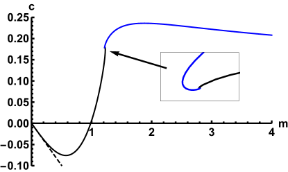
Figure 1: In this figure we plot the condensate parameter $c$ versus the mass parameter $m$. The solid curves have been found numerically both for black hole embeddings (black curve) and Minkowski embeddings (blue curve). The transition between them occurs at $m\approx 1.23$. The condensate $c$ vanishes for a black hole embedding at approximately $m\approx 0.985$. The dashed linear curve near $m=0$ corresponds to the high temperature analytic result (E.22). The condensate of the Minkowski embeddings with $m\rightarrow\infty$ tends to zero as $c\propto m^{-{14\over 3}}$.

In order to get the embedding function $\eta(u)$ in the whole range of the holographic coordinate $u$ we must solve numerically the Euler-Lagrange equation of motion derived from the action (3.30). For a black hole embedding we must impose regularity conditions at the horizon $u=1$, which are easily seen to be:

$$\eta(u=1)\,=\,\eta_{h}\,\,,\qquad\qquad\dot{\eta}(u=1)\,=\,0\,\,,$$ (3.32)

where $\eta_{h}$ is an IR constant which determines the UV constants $m$ and $c$. By varying $\eta_{h}$ we get a relation $c=c(m)$, which determines the condensate as a function of the quark mass at fixed temperature or, equivalently, the condensate as a function of the temperature at fixed $m_{q}$. The corresponding results are plotted in Fig. 1. We notice that $c$ is negative for small $m$ (or large $T$), vanishes near $m\approx 1$ and becomes positive for larger values of $m$. For high temperatures (or low $m$) the embedding function $\eta$ remains small for all values of the holographic coordinate $u$ and the equation for the embedding can be linearized and solved analytically. This analysis is presented in detail in Appendix E. We find that $c$ decreases linearly with $m$ ($c\approx-0.198m$, see (E.22)). This result is in good agreement with the numerical results, as shown in Fig. 1.

We want now to address the problem of determining the thermodynamic functions of the probe. The first step in this analysis is finding the free energy density $F$ of the D7-brane. The expression of $F$ can be obtained from the Euclidean on-shell action of the brane, which is divergent and should be regulated appropriately by adding a suitable boundary term. Indeed, plugging the UV behavior (3.31) into the right-hand side of (3.30), we find that ${\cal I}_{bulk}$ diverges in the UV as:

$${\cal I}_{bulk}\Big{|}_{div} = \int^{u_{max}}du\Big{[}u^{{7\over 2}}\,+\,{2\over 5}\,u^{-{1\over 4}}\,-\,{10\over 9}\,m^{2}\,u^{{3\over 2}}\,+\,{m^{4}\over 9}\,u^{-{1\over 2}}\Big{]}$$ (3.33)

$$= {2\over 9}\,u_{max}^{{9\over 2}}\,+\,{8\over 15}\,u_{max}^{{3\over 4}}\,-\,{4\,m^{2}\over 9}\,u_{max}^{{5\over 2}}\,+\,{2\over 9}\,m^{4}\,u_{max}^{{1\over 2}}\,\,.$$

It is quite instructive to compare (3.33) to the behavior (3.8) for the SUSY embedding at zero temperature. The three terms in (3.8) correspond to the first, third, and fourth terms in (3.33) (take into account that $r_{max}\sim u_{max}^{9/8}$). The second term in (3.33) is independent of the embedding and is due to the finite temperature.

To construct a boundary action that cancels the divergences of ${\cal I}_{bulk}$ we first consider the boundary metric at $u=u_{max}$

$$ds^{2}(\gamma)\,\sim\,u_{max}^{{2\over b}}\,\tilde{f}^{{6\over 5}}(u_{max})\,\Big{[}-{f^{2}(u_{max})\over\tilde{f}^{2}(u_{max})}(dx^{0})^{2}\,+\,(dx^{1})^{2}\,+\,(dx^{2})^{2}\,+\,e^{-2\phi}\,(dx^{3})^{2}\Big{]}\,\,.$$ (3.34)

It follows that:

$$e^{\phi}\,\sqrt{-\det\gamma}\,=\,u_{max}^{{4\over b}}\tilde{f}^{{7\over 5}}(u_{max})\,f(u_{max})\,\,.$$ (3.35)

We want the renormalized action to vanish for the SUSY embeddings at $T=0$. To fulfill this requirement we notice that the on-shell action of such embeddings depends on $\eta$ as $\cos^{4}\chi=(1-\eta^{2})^{2}$ evaluated at the boundary (see (3.6)). Taking this fact into account, let us write the boundary action as:

$${\cal I}_{bdy}\,=\,\alpha\,f^{\beta_{1}}\,\tilde{f}^{\beta_{2}}\,e^{\phi}\,\sqrt{-\det\gamma}\,\,(1-\eta^{2})^{2}\,\Big{|}_{u=u_{max}}\,\,,$$ (3.36)

where $\alpha$, $\beta_{1}$, and $\beta_{2}$ are constants to be determined by imposing the condition that ${\cal I}_{bulk}+{\cal I}_{bdy}$ is finite as $u_{max}\rightarrow\infty$. We have included in (3.36) a prefactor containing powers of the functions $f$ and $\tilde{f}$ to take into account the redshift occurring at $T\not=0$ due to the emblackening factor of the metric. Actually, this term is needed to cancel the second term on the right-hand side of (3.33). Plugging in the UV behavior of the embedding function $\eta$ (eq. (3.31)), we find

$${\cal I}_{bdy}\,=\,\alpha\,\Big{[}u_{max}^{{9\over 2}}\,+\,\Big{(}{2\over 5}\,-\,\beta_{1}+\beta_{2}\Big{)}\,u_{max}^{{3\over 4}}\,-\,2m^{2}\,u_{max}^{{5\over 2}}\,+\,m^{4}\,u_{max}^{{1\over 2}}\,-\,4\,m\,c\,\Big{]}\,\,.$$ (3.37)

By requiring the cancellation of the leading term of ${\cal I}_{bulk}+{\cal I}_{bdy}$, we fix the value of the constant $\alpha$ to be:

$$\alpha\,=\,-{2\over 9}\,\,.$$ (3.38)

Moreover, the cancellation of the $u_{max}^{{3\over 4}}$ term requires that:

$$\beta_{2}-\beta_{1}\,=\,2\,\,.$$ (3.39)

Using these values of the constants, we can write ${\cal I}_{bdy}$ as:

$${\cal I}_{bdy}\,=\,-{2\over 9}\,u_{max}^{{1\over 2}}\,(u_{max}^{2}-m^{2})^{2}-\,{8\over 15}\,u_{max}^{{3\over 4}}\,+\,{8\over 9}\,m\,c\,\,.$$ (3.40)

Notice also that taking the solution $\beta_{2}=-\beta_{1}=1$ of (3.39), the boundary action can be written in terms of the emblackening factor $B$ as:

$${\cal I}_{bdy}\,=\,-{2\over 9}\,{e^{\phi}\over\sqrt{B}}\,\sqrt{-\det\gamma}\,\,(1-\eta^{2})^{2}\,\Big{|}_{u=u_{max}}\,\,.$$ (3.41)

Let us rewrite the divergent terms on the right-hand side of (3.40) as:

$$-{2\over 9}u_{max}^{{1\over 2}}(u_{max}^{2}-m^{2})^{2}=-{1\over 9}\int_{u_{min}}^{u_{max}}{(u^{2}-m^{2})(9u^{2}-m^{2})\over u^{{1\over 2}}}du-{2\over 9}u_{min}^{{1\over 2}}(u_{min}^{2}-m^{2})^{2}$$

$$-{8\over 15}\,u_{max}^{{3\over 4}}\,=\,-{2\over 5}\,\int_{u_{min}}^{u_{max}}\,u^{-{1\over 4}}\,du\,-{8\over 15}\,u_{min}^{{3\over 4}}\ .$$ (3.42)

Using this result, we can write ${\cal I}_{bdy}$ as the following integral:

$${\cal I}_{bdy} = -\int_{u_{min}}^{u_{max}}{du\over\sqrt{u}}\Big{[}{1\over 9}\,(u^{2}-m^{2})(9u^{2}-m^{2})+{2\over 5}u^{{1\over 4}}\Big{]}$$ (3.43)

$$-{2\over 9}\,u_{min}^{{1\over 2}}\,(u_{min}^{2}-m^{2})^{2}\,-\,{8\over 15}\,u_{min}^{{3\over 4}}\,+\,{8\over 9}\,m\,c\,\,.$$

The free energy density of the probe is given by:

$${F\over{\cal N}} = {\cal I}_{bulk}\,+\,{\cal I}_{bdy}$$ (3.44)

$$= {\cal G}(m)-{2\over 9}u_{min}^{{1\over 2}}(u_{min}^{2}-m^{2})^{2}-{8\over 15}u_{min}^{{3\over 4}}+{8\over 9}\,m\,c\,\,,$$

where ${\cal G}(m)$ is the following integral:

$${\cal G}(m)=\int_{u_{min}}^{\infty}{du\over\sqrt{u}}\Big{[}u^{4}\,f\,\tilde{f}^{{7\over 5}}\,(1-\eta^{2})\,\sqrt{1-{\eta^{2}\over 9}}\,\sqrt{1-\eta^{2}+{8u^{2}\over 9}\,\dot{\eta}^{2}}$$

$$\qquad\qquad\qquad\qquad\qquad\qquad-\,{1\over 9}(u^{2}-m^{2})(9u^{2}-m^{2})\,-\,{2\over 5}\,u^{{1\over 4}}\Big{]}\ .$$ (3.45)

We have extended the upper limit of integration to $\infty$ since it is a convergent integral. For black hole embeddings, $u_{\min}=1$ in (3.44) and (3.45).

Once $F$ is known, we can obtain the other thermodynamic functions by using the standard relations between them. For example, the entropy density $s$ of the probe can be computed as:

$$s\,=\,-{\partial F\over\partial T}\,=\,-{F\over{\cal N}}\,{\partial{\cal N}\over\partial T}\,-\,{\cal N}\,{\partial\over\partial T}\Big{(}{F\over{\cal N}}\Big{)}\,\,.$$ (3.46)

Since ${\cal N}\sim T^{4}$, $\partial_{T}{\cal N}=4{\cal N}/T$ and therefore

$$s\,=\,-{4\,F\over T}\,-\,{\cal N}\,{\partial\over\partial T}\Big{(}{F\over{\cal N}}\Big{)}\,\,.$$ (3.47)

Let us now calculate the second term in this expression

$${\partial\over\partial T}\Big{(}{F\over{\cal N}}\Big{)}\,=\,{\partial\over\partial m}\Big{(}{F\over{\cal N}}\Big{)}\,{\partial m\over\partial T}\,=\,-{b\,m\over T}\,{\partial\over\partial m}\Big{(}{F\over{\cal N}}\Big{)}\,\,,$$ (3.48)

where we took into account that, for fixed quark mass $m_{q}$, the mass parameter $m$ behaves as $m\approx T^{-b}$ (B.8). The derivative of $F/{\cal N}$ with respect to $m$ can be extracted from (B.20), yielding

$$T\,{s\over{\cal N}}\,=\,-4\,{F\over{\cal N}}\,-\,{160\over 81}\,c\,m\,\,,$$ (3.49)

where $F/{\cal N}$ can be obtained from (3.44) for black hole embeddings or from (3.66) for Minkowski embeddings. The internal energy $E$ is given by $E=F+Ts$:

$${E\over{\cal N}}\,=\,-3\,{F\over{\cal N}}\,-\,{160\over 81}\,c\,m\,\,.$$ (3.50)

Let us next compute the heat capacity, defined as:

$$c_{v}\,=\,{\partial E\over\partial T}\,\,.$$ (3.51)

Proceeding as with $F$ to compute this derivative, we get:

$$T\,{c_{v}\over{\cal N}} = -12\,{F\over{\cal N}}\,\,-\,{160\over 729}\,\Big{[}1\,-\,8\,{\partial\log c\over\partial\log m}\Big{]}\,c\,m$$ (3.52)

$$= 3\,T\,{s\over{\cal N}}\,+\,{320\over 729}\Big{[}13\,+\,4\,{\partial\log c\over\partial\log m}\Big{]}\,c\,m\ .$$ (3.53)

From the behavior of $F$ at high temperature obtained in Appendix E, (eq. (E.36)), it is immediate to find the leading behavior of $s$, $E$, and $c_{v}$:

$$\lim_{m\rightarrow 0}\,T\,{s\over{\cal N}}\,=\,{32\over 9}\,2^{{2\over 5}}\,\,,\qquad\qquad\lim_{m\rightarrow 0}\,{E\over{\cal N}}\,=\,{8\over 3}\,2^{{2\over 5}}\,\,,\qquad\qquad\lim_{m\rightarrow 0}\,T\,{c_{v}\over{\cal N}}\,=\,{32\over 3}\,2^{{2\over 5}}\,\,.$$ (3.54)

We have checked this high temperature behavior numerically (see Fig. 2).

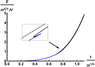
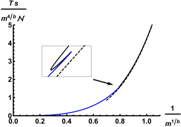
Figure 2: In these plots we represent the free energy density, internal energy density, and entropy density as a function of $m^{-{1\over b}}\sim T$. Notice that the normalization factor $m^{{4\over b}}\,{\cal N}$ is independent of the temperature. The continuous black (blue) curve corresponds to black hole (Minkowski) embeddings. Near the transition point the expected swallowtail behavior is obtained. The dashed curves are the result of the analytic high temperature calculation of Appendix E.

3.2.2 Minkowski embeddings

The $\eta=\eta(u)$ parametrization is convenient for the black hole embeddings. For Minkowski embeddings, Cartesian-like coordinates $(\rho,P)$ are better suited. They are defined in terms of $u$ and $\chi$ as follows:

$$P\,=\,u\sin\chi\,\,,\qquad\qquad\rho\,=\,u\cos\chi\,\,.$$ (3.55)

The inverse relation is:

$$u\,=\,\big{[}\rho^{2}\,+\,P^{2}\big{]}^{{1\over 2}}\,\,,\qquad\qquad\tan\chi\,=\,{P\over\rho}\,\,.$$ (3.56)

When using these variables, we parametrize our embeddings by a function $P=P(\rho)$, then

$${dr\over r\,\sqrt{B}}\,=\,{1\over b}\,{du\over u}\,=\,{1\over b}\,{\rho+P\,P^{\prime}\over\rho^{2}\,+\,P^{2}}\,d\rho\,\,,\qquad\qquad d\chi\,=\,{\rho\,P^{\prime}\,-\,P\over\rho^{2}+P^{2}}\,d\rho\,\,,$$ (3.57)

where $P^{\prime}=dP/d\rho$. Let us now write down the induced metric on the worldvolume. Taking into account that:

$${h^{{1\over 2}}\,dr^{2}\over B}\,+\,h^{{1\over 2}}e^{2g}\,(d\chi)^{2}\,=\,{R^{2}\over b^{2}(\rho^{2}+P^{2})^{2}}\,\Big{[}(\rho+P\,P^{\prime})^{2}\,+\,b\,(\rho\,P^{\prime}-P)^{2}\Big{]}\,d\rho^{2}\,\,,$$ (3.58)

as well as:

$$r\,=\,{r_{h}\over 2^{{3\over 5}}}\,\big{[}\rho^{2}+P^{2}\big{]}^{{1\over 2b}}\,\tilde{f}^{{3\over 5}}\,\,,\qquad\qquad\cos^{2}\chi\,=\,{\rho^{2}\over\rho^{2}+P^{2}}\,\,,$$ (3.59)

we get:

$$ds_{8}^{2} = {r_{h}^{2}\over 2^{{6\over 5}}\,R^{2}}\big{[}\rho^{2}+P^{2}\big{]}^{{1\over b}}\,\tilde{f}^{{6\over 5}}\Big{[}-{f^{2}\over\tilde{f}^{2}}(dx^{0})^{2}+(dx^{1})^{2}+(dx^{2})^{2}+e^{-2\phi}\,(dx^{3})^{2}\Big{]}$$ (3.60)

$$+{R^{2}\over b^{2}(\rho^{2}+P^{2})^{2}}\Big{[}(\rho+P\,P^{\prime})^{2}\,+\,b\,(\rho\,P^{\prime}-P)^{2}\Big{]}d\rho^{2}$$

$$+{R^{2}\over 4b}\,{\rho^{2}\over\rho^{2}+P^{2}}\Big{[}(\omega^{1})^{2}+(\omega^{2})^{2}\,+\,\Big{(}1+{1-b\over b}\,{\rho^{2}\over\rho^{2}+P^{2}}\Big{)}(\omega^{3})^{2}\,\Big{]}\,\,.$$

In this expression $\tilde{f}$ and $f$ should be understood as the functions:

$$\tilde{f}\,=\,1+(\rho^{2}+P^{2})^{-{15\over 8}}\,\,,\qquad\qquad f\,=\,1-(\rho^{2}+P^{2})^{-{15\over 8}}\,\,.$$ (3.61)

It follows that the DBI Lagrangian density in these variables is:

$${\cal L}\,\sim\,-\rho^{3}\,\tilde{f}^{{7\over 5}}\,f\,(\rho^{2}+P^{2})^{-{3\over 4}}\,\Big{(}\rho^{2}+{8\over 9}\,P^{2}\Big{)}^{{1\over 2}}\,\Big{[}(\rho+P\,P^{\prime})^{2}\,+\,{8\over 9}\,(\rho\,P^{\prime}-P)^{2}\Big{]}^{{1\over 2}}\,\,.$$ (3.62)

Let us now study the free energy $F$ in these variables. First of all, let us write the bulk on-shell action as:

$${\cal I}_{bulk}\,=\,\int_{0}^{\rho_{max}}\,d\rho\,\rho^{3}\,\,\tilde{f}^{{7\over 5}}\,f\,(\rho^{2}+P^{2})^{-{3\over 4}}\,\Big{(}\rho^{2}+{8\over 9}\,P^{2}\Big{)}^{{1\over 2}}\,\Big{[}(\rho+P\,P^{\prime})^{2}\,+\,{8\over 9}\,(\rho\,P^{\prime}-P)^{2}\Big{]}^{{1\over 2}}\,\,.$$ (3.63)

This action diverges at the UV. To characterize this divergence, we use the UV behavior of the embedding function $P(\rho)$:

$$P=m\,+\,{c\over\rho^{{5\over 2}}}\,+\,\ldots\,\,,\qquad\qquad(\rho\rightarrow\infty)\,\,.$$ (3.64)

Following similar steps as in Section 3.2.1, it is straightforward to find the regulator:

$${\cal I}_{bdy}\,=\,-\int_{0}^{\rho_{max}}d\rho{\rho^{3}\,\tilde{f}_{m}^{{7\over 5}}\over\big{(}\rho^{2}+m^{2}\big{)}^{{3\over 4}}}\Bigg{(}\rho^{2}\,+\,{8\over 9}\,m^{2}\,-\,{\rho^{2}\,-\,{8\over 9}\,m^{2}\over\big{(}\rho^{2}+m^{2}\big{)}^{{15\over 8}}}\,\Bigg{)}\,-\,{m\,c\over 9}\,\,.$$ (3.65)

Alternatively, one can simply perform the change of variables on (3.43) to land on (3.65). It follows that the free energy $F$ can be represented as:

$${F\over{\cal N}} = \int_{0}^{\infty}d\rho\,\rho^{3}\,\Bigg{[}\,{\tilde{f}^{{7\over 5}}\,f\,\over(\rho^{2}+P^{2})^{{3\over 4}}}\,\Big{(}\rho^{2}+{8\over 9}\,P^{2}\Big{)}^{{1\over 2}}\,\Big{[}(\rho+P\,P^{\prime})^{2}\,+\,{8\over 9}\,(\rho\,P^{\prime}-P)^{2}\Big{]}^{{1\over 2}}$$ (3.66)

$$-\,{\tilde{f}_{m}^{{7\over 5}}\over\big{(}\rho^{2}+m^{2}\big{)}^{{3\over 4}}}\Bigg{(}\rho^{2}\,+\,{8\over 9}\,m^{2}\,-\,{\rho^{2}\,-\,{8\over 9}\,m^{2}\over\big{(}\rho^{2}+m^{2}\big{)}^{{15\over 8}}}\,\Bigg{)}\,\Bigg{]}-\,{m\,c\over 9}\ .$$

As a highly non-trivial check of this expression, we have verified numerically that $F$ vanishes when $m\rightarrow\infty$ (see Fig. (2)). The other thermodynamic functions $S$, $E$, and $c_{v}$ can be obtained from the free energy $F$ by using (3.49), (3.50), and (3.53), respectively. The corresponding numerical values are presented in Fig. 2.

4 Non-zero density

Let us now explore the D3-D5-D7 system at non-zero charge density. To simplify our analysis we restrict ourselves to the case in which the embedding function $\chi$ is zero which, according to the holographic dictionary, corresponds to having massless quarks. Recall that $\chi=0$ solves trivially the equation of motion (2.20). Moreover, when $\chi=0$ eq. (2.19) yields the following value for the radial derivative of the worldvolume gauge field potential $A_{t}$:

$$A_{t}^{\prime}={e^{{\phi\over 2}}\,d\over\sqrt{d^{2}+r^{6}\,e^{-\phi}}}\ .$$ (4.1)

By the AdS/CFT dictionary, the chemical potential is given by the UV value of $A_{t}$:

$$\mu\equiv A_{t}(r\rightarrow\infty)=\,d\,\int_{r_{h}}^{\infty}\,{e^{{\phi\over 2}}\over\sqrt{d^{2}+r^{6}\,e^{-\phi}}}\ .$$ (4.2)

The last equality follows for the black hole embeddings of the D7-brane, since the temporal part of the background gauge potential has to vanish at the horizon. Notice that in the current case, at finite density, the only possible embeddings are those that enter into the black hole. At zero density, but at finite chemical potential, there is the possibility of considering Minkowski embeddings in which case one needs to allow non-zero IR values of the gauge potential [66, 67].

Using the value of the dilaton $\phi$ for our background (2.6), we can directly perform the integration in (4.2), yielding

$$\mu=\Big{(}{3\over 4\,Q_{f}}\Big{)}^{{1\over 2}}\,\gamma\,d^{{1\over 2}}-{3\over 4}\,\Big{(}{3\over 4\,Q_{f}}\Big{)}^{{1\over 3}}\,r_{h}^{{4\over 3}}\,F\Big{(}{1\over 4},{1\over 2};{5\over 4};-\Big{(}{4\,Q_{f}\over 3}\Big{)}^{{2\over 3}}\ ,{r_{h}^{{16\over 3}}\over d^{2}}\Big{)}$$ (4.3)

where $\gamma$ is the following constant:

$$\gamma={3\over\sqrt{\pi}}\,\Big{[}\Gamma\Big{(}{5\over 4}\Big{)}\Big{]}^{2}\ .$$ (4.4)

For later purposes we also define a function $H$ as follows

$$H\equiv r^{6}\,e^{-\phi}\ .$$ (4.5)

4.1 Stiffness at zero temperature

Before discussing the excitation spectrum of our system it is useful to start with computing the stiffness at zero temperature. This is given by the following thermodynamic derivative at fixed entropy density

$$u_{i}^{2}=\frac{\partial p_{i}}{\partial\epsilon}\Big{|}_{s}\,\,,$$ (4.6)

where $p_{i}$ is the pressure along direction $x^{i}$. At zero temperature this typically agrees with $\frac{\partial p_{i}}{\partial\epsilon}\Big{|}_{T}$ [68] that we aim to compute. With an abuse of language we follow the existing literature and henceforth call (4.6) the speed of first sound.

Let us now take $T=r_{h}=0$ in our equations and let us examine the thermodynamics of the probe at zero temperature. When $r_{h}=0$ the second term in (4.3) vanishes and $\mu$ is related to the density $d$ as follows:

$$\mu\,=\,\Big{(}{3\over 4\,Q_{f}}\Big{)}^{{1\over 2}}\,\gamma\,d^{{1\over 2}}\,\,.$$ (4.7)

Then, the on-shell action is:

$$S_{on-shell}\,=\,-{\cal N}\,V_{4}\,\int_{0}^{\infty}\,dr\,{r^{3}\,\sqrt{H}\over\sqrt{d^{2}+H}}\,\,,$$ (4.8)

where $V_{4}$ is the volume of our system in the four-dimensional Minkowski space-time. Since the function $H$ is given by:

$$H\,=\,\alpha\,r^{{16\over 3}}\,\,,\qquad\qquad\qquad\alpha\equiv\Big{(}{4Q_{f}\over 3}\Big{)}^{{2\over 3}}\,\,,$$ (4.9)

the on-shell action is divergent and must be regulated by subtracting the action at zero density. We get:

$$S_{on-shell}^{reg}\,=\,-{\cal N}\,V_{4}\,\int_{0}^{\infty}\,dr\,r^{3}\,\Big{[}{\sqrt{H}\over\sqrt{d^{2}+H}}-1\Big{]}={1\over 3}\,{\cal N}\,V_{4}\,\gamma\,\Big{(}{3\over 4\,Q_{f}}\Big{)}^{{1\over 2}}\,d^{{3\over 2}}\ .$$ (4.10)

The grand potential $\Omega$ is just $\Omega=-S_{on-shell}^{reg}$. Therefore:

$$\Omega\,=\,-{1\over 3}\,{\cal N}\,V_{4}\,\gamma\,\Big{(}{3\over 4\,Q_{f}}\Big{)}^{{1\over 2}}\,d^{{3\over 2}}\,=\,-{1\over 3}\,{{\cal N}\,V_{4}\over\gamma^{2}}\,\Big{(}{4Q_{f}\over 3}\Big{)}\,\mu^{3}\,\,.$$ (4.11)

From $\Omega$ we get the density $\rho$ as:

$$\rho\,=\,-{1\over V_{4}}\,{\partial\Omega\over\partial\mu}\,=\,{\cal N}\,d\,\,,$$ (4.12)

as well as the energy density $\epsilon$:

$$\epsilon\,=\,{\Omega\over V_{4}}\,+\,\mu\,\rho\,=\,{2\over 3}\,{\cal N}\,\gamma\,\Big{(}{3\over 4\,Q_{f}}\Big{)}^{{1\over 2}}\,d^{{3\over 2}}\,=\,-\,{2\,\Omega\over V_{4}}\,\,.$$ (4.13)

In order to obtain the pressures along the different directions, let us put the system in a box of sides $L_{1}$, $L_{2}$, and $L_{3}$ in the directions of $x^{1}$, $x^{2}$, and $x^{3}$ respectively. Then, the pressure along the $i^{th}$ direction is given by:

$$p_{i}\,=\,-{L_{i}\over V_{4}}\,{\partial\Omega\over\partial L_{i}}\,\,,\qquad\qquad(i=1,2,3)\,\,.$$ (4.14)

The grand potential $\Omega$ is an extensive quantity which clearly depends linearly on $L_{1}$ and $L_{2}$. Therefore, if $p_{\parallel}$ refers to the pressure in the $x^{1}\,x^{2}$ plane, we have:

$$p_{\parallel}\,=\,-{\Omega\over V_{4}}\,=\,{\epsilon\over 2}\,\,.$$ (4.15)

It follows that the corresponding in-plane speed of sound is:

$$u_{\parallel}^{2}\,=\,{\partial p_{\parallel}\over\partial\epsilon}\,=\,{1\over 2}\,\,.$$ (4.16)

In section 4.2.1, by studying the fluctuations of the probe D7-brane, we will show that this value of $u_{\parallel}$ coincides with the value of the speed of the in-plane zero sound.

The result in (4.16) matches the value corresponding to a conformal theory in 2d and not that of 3d. Notice that at finite chemical potential there are plenty of examples in holography where one can exceed the conformal value [69, 68, 70], as long as the conformal symmetry is broken. Here the mechanism is quite different and can be associated with the presence of the defect instead of some intrinsic energy scale. At vanishing chemical potential there are also other mechanisms that lead to stiff equations of state: brane intersections with non-AdS asymptotics [72, 71, 73], softly broken translational symmetry [74], having non-relativistic scaling symmetries [76, 75], dynamical magnetic fields [77], and those obtained from double trace deformations [78].

The dependence of $\Omega$ on $L_{3}$ is not clear since $Q_{f}$ is proportional to the density $N_{f}$ of D5-branes smeared along $x^{3}$. Therefore, the calculation of the thermodynamic derivative (4.14) is far from obvious in this case. Actually, we will verify in section (4.2.2) that the dispersion relation of the off-plane modes in the zero sound channel is quite different from the ones corresponding to the sound modes propagating along the plane directions.

4.2 Zero sound

Let us now turn to discussing the collective phenomena that arise from fluctuating the fields on the worldvolume of the D7-brane. In the field theory dual, these excitations are density waves which correspond to quasinormal modes on the gravity side. We are only discuss vector fields, focusing solely on s-waves. Thus, we suppress the dependence on the internal part of the geometry. We start the analysis at zero temperature, where we can obtain analytic results. In the subsequent section, we instead focus on the high temperature result, which is also amenable for analytic treatment. In between there is the regime of finite temperature where we need to resort to numerical analysis, which accurately interpolates the limiting cases.

Let us thus begin by considering our system at exactly zero temperature. Here the dominant mode is the so-called holographic zero sound [79] which is a pretty robust collective excitation mode persisting to finite temperature [80]. Many other aspects of the holographic zero sound mode have been discussed in various contexts [81, 82, 73, 83, 84, 85, 76, 86, 87, 88, 89, 90, 91, 92, 93, 94, 95, 96, 97, 98, 99, 72, 100, 71, 75, 42, 16]. To study these modes we perturb the worldvolume gauge potential as follows

$$A\,=\,A^{(0)}+\delta A\ ,$$ (4.17)

where $A^{(0)}$ is the gauge field of (4.1) and $\delta A$ is a small perturbation about the equilibrium value. We Fourier transform to momentum space:

$$\delta A_{\mu}\,=\,a_{\mu}(\,r,\omega,\vec{k}\,)\,e^{-i\omega t\,+\,i\vec{k}\cdot\vec{x}}\ .$$ (4.18)

The equations of motion for the fluctuations can be obtained by perturbing the DBI action around the configuration with $\chi=0$ and $A=A^{(0)}$. The derivation of these equations is done in Appendix F. We work in the radial gauge by setting $a_{r}=0$. We also introduce a gauge-invariant combination, the electric field:

$$\vec{E}\,=\,\vec{k}\,a_{t}\,+\,\omega\,\vec{a}\ .$$ (4.19)

In what follows we consider the case in which $\vec{a}$ and $\vec{k}$ are parallel. There are then two possibilities depending on the direction of wave propagation. When $\vec{k}$ is oriented along the $(x^{1},x^{2})$ plane we call it “in-plane”, whereas the “off-plane” waves propagate along $x^{3}$. We distinguish between these two cases in the subsequent sections.

4.2.1 In-plane zero sound

Let us consider the in-plane fluctuations at zero temperature. For concreteness, we assume that $\vec{k}=k_{\parallel}\vec{e}_{x^{1}}$ is directed along $x^{1}\equiv x$. The corresponding equation for $E\equiv k_{\parallel}\,a_{t}\,+\,\omega\,a_{x}$ is worked out in the appendix, c.f. (F.24), and takes the following form

$$E^{\prime\prime}\,+\,\partial_{r}\log\Bigg{[}{e^{-{\phi\over 2}}\,\big{(}H+d^{2}\big{)}^{{3\over 2}}\,B\over(\omega^{2}-k_{\parallel}^{2}\,B)\,H\,+\,\omega^{2}\,d^{2}}\Bigg{]}\,E^{\prime}\,+\,{h\over B^{2}}\,{(\omega^{2}-k_{\parallel}^{2}\,B)\,H\,+\,\omega^{2}\,d^{2}\over H+d^{2}}\,E\,=\,0\,\,.$$ (4.20)

Since in this section we are interested in the $T=0$ case, we take $B=1$ from now on. We first study (4.20) near the horizon $r=0$, where it takes the form:

$$E^{\prime\prime}\,-\,{1\over 3\,r}\,E^{\prime}\,+\,{R^{4}\omega^{2}\over r^{4}}\,E\,=\,0\,\,.$$ (4.21)

The solution of this near-horizon equation with infalling boundary conditions at $r=0$ can be written in terms of a Hankel function of the first type:

$$E(r)\sim r^{{2\over 3}}\,H_{{2\over 3}}^{(1)}\Big{(}{R^{2}\,\omega\over r}\Big{)}\ .$$ (4.22)

When the index $\nu$ of $H_{\nu}^{(1)}$ is not an integer the Hankel function has the following expansion near the origin:

$$H_{\nu}^{(1)}(\alpha x)=-{2^{\nu}\,\Gamma(\nu)\over\pi\,\alpha^{\nu}}\,i\,\Big{[}{1\over x^{\nu}}\,+\,{\pi\over\Gamma(\nu)\,\Gamma(\nu+1)}\,\Big{(}{\alpha\over 2}\Big{)}^{2\nu}\,\Big{(}i\,-\,\cot(\pi\nu)\Big{)}\,x^{\nu}\,+\,\ldots\Big{]}\,\,.$$ (4.23)

Let us then expand the near-horizon electric field at low frequency as:

$$E(r)\sim A\,\Big{[}1\,+\,{\cal C}\,\omega^{-{4\over 3}}\,r^{{4\over 3}}\,+\,\cdots\Big{]}\ ,$$ (4.24)

where ${\cal C}$ is a constant:

$${\cal C}\,=\,{\sqrt{3}-3i\over 6\pi}\,\Gamma^{2}\Big{(}{2\over 3}\Big{)}\,\Big{(}{2\over R^{2}}\Big{)}^{{4\over 3}}\ .$$ (4.25)

Let us now perform the two limits (near-horizon and low frequency) in opposite order. At low frequency and momentum we can neglect the last term in (4.20) and the equation can be integrated once to give:

$$E^{\prime}\,=\,c_{E}\,\omega^{2}\,{e^{{\phi\over 2}}\over(H+d^{2})^{{1\over 2}}}\,-\,c_{E}\,k_{\parallel}^{2}\,{e^{{\phi\over 2}}\,H\over(H+d^{2})^{{3\over 2}}}\,\,,$$ (4.26)

where $c_{E}$ is a constant. To perform a second integration, let us define the rescaled density $\tilde{d}$ as follows:

$$\tilde{d}^{2}\,=\,{d^{2}\over\alpha}\,\,,$$ (4.27)

where $\alpha$ is the quantity defined in (4.9). We also define the integrals $I(r)$ and $J(r)$ as:

$$I(r)\,\equiv\,\int_{r}^{\infty}\,{\rho^{{1\over 3}}\,d\rho\over(\rho^{{16\over 3}}+\tilde{d}^{\,2})^{{1\over 2}}}\,\,,\qquad\qquad J(r)\,\equiv\,\int_{r}^{\infty}\,{\rho^{{17\over 3}}\,d\rho\over(\rho^{{16\over 3}}+\tilde{d}^{\,2})^{{3\over 2}}}\,\,.$$ (4.28)

Then, $E(r)$ at low frequency can be written as:

$$E(r)\,=\,E_{0}\,-\,{c_{E}\over\alpha}\,\omega^{2}\,I(r)\,+\,{c_{E}\over\alpha}\,k_{\parallel}^{2}\,J(r)\,\,,$$ (4.29)

where $E_{0}$ is the value of $E$ at the UV boundary: $E_{0}\,=\,E(r\rightarrow\infty)$.

The integrals $I(r)$ and $J(r)$ are special cases of the integrals that we define and inspect in the Appendix G, see (G.2) and (G.5), respectively. More precisely, the relationships are:

$$I(r)\,=\,I_{{1\over 3},{16\over 3}}(r)\,\,,\qquad\qquad J(r)\,=\,J_{{17\over 3},{16\over 3}}(r)\ .$$ (4.30)

According to the general formulas (G.3) and (G.6) these integrals behave near $r=0$ as:

$$I(r)\approx\gamma\,\tilde{d}^{-{1\over 2}}\,-\,{3\over 4\tilde{d}}\,r^{{4\over 3}}\,\,,\qquad\qquad\qquad\qquad J(r)\approx{\gamma\over 2}\,\tilde{d}^{-{1\over 2}}\,-\,{3\over 20}\,{r^{{20\over 3}}\over\tilde{d}^{\,3}}\ ,$$ (4.31)

where $\gamma$ is the constant defined in (4.4). Therefore, $E(r)$ behaves near the horizon as:

$$E(r)\,\approx\,E_{0}\,+\,{3\,c_{E}\over 4\alpha}\,{\omega^{2}\over\tilde{d}}\,r^{{4\over 3}}\,-\,{c_{E}\,\gamma\over\alpha\,\sqrt{\tilde{d}}}\,\Big{(}\omega^{2}-{1\over 2}\,k_{\parallel}^{2}\Big{)}\,\,.$$ (4.32)

Let us now compare (4.24) and (4.32). By looking at the terms depending on $r$ we get:

$$A\,=\,{3\,c_{E}\over 4\,\alpha\,{\cal C}}\,{\omega^{{10\over 3}}\over\tilde{d}}\,\,.$$ (4.33)

By comparing the constant terms and using (4.33) we find:

$$E_{0}\,=\,{c_{E}\,\gamma\over\alpha\,\sqrt{\tilde{d}}}\,\Big{(}\omega^{2}-{1\over 2}\,k_{\parallel}^{2}\Big{)}\,+\,{3\,c_{E}\over 4\,\alpha\,{\cal C}}\,{\omega^{{10\over 3}}\over\tilde{d}}~{}.$$ (4.34)

By imposing Dirichlet conditions at the UV boundary, i.e. $E_{0}=0$, we get the following dispersion relation:

$${1\over 2}\,k_{\parallel}^{2}\,-\,\omega^{2}\,=\,{3\over 4\,\gamma\,{\cal C}}\,{\omega^{{10\over 3}}\over\sqrt{\tilde{d}}}\,\,.$$ (4.35)

In Fig. 3, where we have used the reduced quantities defined in (4.79), we compare this to the numerical results and find that they are accurately captured at small temperature. We choose to represent the dispersion in the case where we keep frequency real and take complex momentum. Then a convenient way to display the result is to plot the ratio

$$\frac{{\rm{Re}}k_{\parallel}}{{\rm{Im}}k_{\parallel}}=\frac{\sqrt{3}g}{g+\omega^{-4/3}}\left[\sqrt{1+\frac{3g^{2}\omega^{20/3}}{(\omega^{2}+g\omega^{10/3})^{2}}}-1\right]^{-1}\ ,\ g\equiv\frac{3\sqrt{3}}{8\gamma}\frac{\pi}{\sqrt{\tilde{d}}\;\Gamma(2/3)^{2}}\left(R^{2}/2\right)^{4/3}\ ,$$ (4.36)

which readily follows from (4.35). In the limit of high frequency this ratio asymptotes to $\sqrt{3}$. We note that at any non-zero temperature, the zero sound is not the dominant mode at small frequency, but the relevant physics is dominated by the diffusion pole discussed in the subsequent section.

Let us then study the dispersion relation at small frequency. At leading order in $\omega$ (4.35) becomes:

$$\omega\,=\,\pm{1\over\sqrt{2}}\,k_{\parallel}\ .$$ (4.37)

We note that this result equals the first sound result (4.16) obtained in the previous section. Note also that we could write the dispersion relation (4.35) in terms of the chemical potential $\mu$ by using the relation:

$$\gamma\,\sqrt{\tilde{d}}\,=\,\Big{(}{4Q_{f}\over 3}\Big{)}^{{1\over 3}}\,\mu\,=\,\sqrt{\alpha}\,\mu\,\,.$$ (4.38)

Let us now find the next order dispersion relation by writing

$$\omega\,=\,{1\over\sqrt{2}}\,k_{\parallel}\,+\,\delta\omega\,\,,$$ (4.39)

and plugging this ansatz in (4.35), we get at first order in $\delta\omega$:

$$\delta\omega\,\approx\,-{3\over 4\sqrt{\alpha}\,{\cal C}\,\mu}\,\Bigg{[}{k_{\parallel}^{{7\over 3}}\over 4\,\cdot 2^{{1\over 6}}}\,+\,{5\cdot 2^{{1\over 3}}\over 6}\,k_{\parallel}^{{4\over 3}}\,\delta\omega\Bigg{]}\,\,.$$ (4.40)

We can now solve for $\delta\omega$ in powers of $k_{\parallel}$. The second term on the RHS is clearly of higher order. Therefore:

$$\delta\omega\,\approx-{3\over 16\cdot 2^{{1\over 6}}}\,{1\over\sqrt{\alpha}\,{\cal C}\,\mu}\,k_{\parallel}^{{7\over 3}}\,=\,-{3\pi\over 64\,\sqrt{2}\,\,\Gamma^{2}\Big{(}{2\over 3}\Big{)}}\,(\sqrt{3}+3\,i)\,{R^{{8\over 3}}\over\sqrt{\alpha}\,\mu}\,k_{\parallel}^{{7\over 3}}\,\,.$$ (4.41)

The imaginary part of this equation gives the attenuation of the in-plane zero sound, namely:

$${\rm Im}\,\omega\,=\,-{9\,\pi\over 64\,\sqrt{2}\,\,\Gamma^{2}\Big{(}{2\over 3}\Big{)}}\,{R^{{8\over 3}}\over\sqrt{\alpha}\,\mu}\,k_{\parallel}^{{7\over 3}}\,\,.$$ (4.42)

Moreover, the higher order correction to ${\rm Re}\,\omega$ is:

$${\rm Re}\,\delta\omega\,=\,-{3\sqrt{3}\,\pi\over 64\,\sqrt{2}\,\,\Gamma^{2}\Big{(}{2\over 3}\Big{)}}\,{R^{{8\over 3}}\over\sqrt{\alpha}\,\mu}\,k_{\parallel}^{{7\over 3}}\,\,.$$ (4.43)

Figure 3: We display the numerical dispersions (red curves) and the approximated dispersions obtained analytically (black dashed curves). On the left we show the results for the in-plane fundamental mode with analytics from (4.35). On the right we show the off-plane fundamental mode with analytics from (4.57). Different curves denote different temperatures: $\log_{10}\hat{d}=1,2,3,4,5,6$ (bottom-up), i.e., from highish to low temperature at fixed density; see (4.79) for the definition of the quantities with hats. All the numerical curves asymptote to unity on the vertical axis that correspond to diffusion poles, marked by blue points. At high frequencies all the curves asymptote to $\sqrt{3}$ and $0$ for the in-plane (left panel) and off-planes (right panel) cases, respectively, though this is not visible in the plotted range.

4.2.2 Off-plane zero sound

We now analyze the case in which $\vec{k}=k_{\perp}\vec{e}_{x^{3}}$ lies in the direction of $x^{3}\equiv z$. The equation for the gauge-invariant combination $E=k_{\perp}\,a_{t}+\omega a_{z}$ has been obtained in (F.28) and can be written as:

$$E^{\prime\prime}\,+\,\partial_{r}\log\Bigg{[}{e^{{3\phi\over 2}}\,\big{(}H+d^{2}\big{)}^{{3\over 2}}\,B\over(\omega^{2}-k_{\perp}^{2}\,B\,e^{2\phi})\,H\,+\,\omega^{2}\,d^{2}}\Bigg{]}\,E^{\prime}\,+\,{h\over B^{2}}\,{(\omega^{2}-k_{\perp}^{2}\,B\,e^{2\phi})\,H\,+\,\omega^{2}\,d^{2}\over H+d^{2}}\,E\,=\,0\,\,.$$ (4.44)

We first analyze (4.44) with $B=1$ near the horizon $r=0$, where it takes the form:

$$E^{\prime\prime}\,+\,{1\over r}\,E^{\prime}\,+\,{R^{4}\omega^{2}\over r^{4}}\,E\,=\,0\,\,.$$ (4.45)

The solution of this near-horizon equation with infalling boundary conditions is:

$$E(r)\sim\,H_{0}^{(1)}\Big{(}{R^{2}\,\omega\over r}\Big{)}\,\,.$$ (4.46)

In order to expand $E$ at low frequencies, we use the expansion of the Hankel function of index zero near the origin:

$$H_{0}^{(1)}(x)\sim{2i\,\gamma_{E}\,+\,\pi\,-\,2i\log 2\over\pi}\,+\,{2i\over\pi}\log x\,\,,$$ (4.47)

where $\gamma_{E}$ is the Euler-Mascheroni constant, yielding

$$E(r)\approx A\,\Big{[}i{\pi\over 2}-\gamma_{E}\,-\,\log{R^{2}\,\omega\over 2}\,+\,\log r\Big{]}\,\,.$$ (4.48)

Let us now redo the computation taking the limits in the opposite order as in the previous subsection. At low frequency we neglect the last term in (4.44), which leads to an equation that can be integrated once as:

$$E^{\prime}\,=\,c_{E}\,\omega^{2}\,{e^{-{3\,\phi\over 2}}\over(H+d^{2})^{{1\over 2}}}\,-\,c_{E}\,k_{\perp}^{2}\,{e^{{\phi\over 2}}\,H\over(H+d^{2})^{{3\over 2}}}\,\,,$$ (4.49)

where $c_{E}$ is a constant. A second integration yields:

$$E(r)\,=\,E_{0}\,-\,c_{E}\,\alpha\,\omega^{2}\,\tilde{I}(r)\,+\,{c_{E}\over\alpha}\,k_{\perp}^{2}\,J(r)\,\,,$$ (4.50)

where $\alpha$ has been defined in (4.9), $J(r)$ is the integral defined in (4.28) and $\tilde{I}(r)$ is a new integral defined as:

$$\tilde{I}(r)\,\equiv\,\int_{r}^{\infty}\,{d\rho\over\rho\,\big{(}\rho^{{16\over 3}}\,+\,\tilde{d}^{2}\big{)}^{{1\over 2}}}={3\over 8\tilde{d}}\,\,{\rm arcsinh}\,\Big{(}{\tilde{d}\over r^{{8\over 3}}}\Big{)}\ .$$ (4.51)

For small $r$ this function behaves as:

$$\tilde{I}(r)\approx{1\over\tilde{d}}\,\Big{[}\log(2\,\tilde{d})^{{3\over 8}}\,-\,\log r\Big{]}\ .$$ (4.52)

Using this result, together with the expansion of $J(r)$ written in (4.31), we get:

$$E(r)\approx E_{0}\,+\,{c_{E}\,\alpha\,\omega^{2}\over\tilde{d}}\,\log r\,-\,c_{E}\,\Big{[}{\alpha\,\log(2\,\tilde{d})^{{3\over 8}}\over\tilde{d}}\,\omega^{2}\,-\,{\gamma\over 2\,\alpha\,\sqrt{\tilde{d}}}\,k_{\perp}^{2}\Big{]}\,\,.$$ (4.53)

Let us now match (4.48) and (4.53). First we identify the terms containing $\log r$, which gives:

$$A\,=\,{c_{E}\,\alpha\,\omega^{2}\over\tilde{d}}\,\,.$$ (4.54)

Using this result, we identify the constant terms and write the UV value of $E$ as:

$$E_{0}\,=\,{c_{E}\,\alpha\,\omega^{2}\over\tilde{d}}\,\Big{[}i{\pi\over 2}-\gamma_{E}\,-\,\log{R^{2}\,\omega\over 2^{{11\over 8}}\,\tilde{d}^{{3\over 8}}}\Big{]}\,-\,{c_{E}\,\gamma\over 2\alpha\,\sqrt{\tilde{d}}}\,k_{\perp}^{2}\,\,.$$ (4.55)

By requiring Dirichlet boundary condition $E_{0}=0$ we arrive at the desired dispersion relation. To simplify the final expression we define the constant ${\cal D}$ as:

$${\cal D}\equiv i{\pi\over 2}-\gamma_{E}\,-\,\log{R^{2}\over 2^{{11\over 8}}\,\tilde{d}^{{3\over 8}}}\ ,$$ (4.56)

so that the dispersion relation can be neatly written as

$$k_{\perp}^{2}\,=\,{2\alpha^{2}\over\gamma\,\sqrt{\tilde{d}}}\,\,\Big{[}{\cal D}\,-\,\log\omega\Big{]}\,\,\omega^{2}\ .$$ (4.57)

In Fig. 3 we compare this to the numerical results and find that they are accurately captured at small temperature. Again, we have chosen to represent the dispersion in the case where momentum is complex while frequency is real. The ratio of the real and imaginary parts of the momentum in this case reads

$$\frac{{\rm{Re}}k_{\perp}}{{\rm{Im}}k_{\perp}}=\frac{\pi}{2}\left[\log(f\omega)+\sqrt{\log^{2}(f\omega)+\frac{\pi^{2}}{4}}\right]^{-1}\ ,\ f\equiv\frac{R^{2}}{2^{11/8}\tilde{d}^{3/8}}e^{\gamma_{E}}\ .$$ (4.58)

In the limit of high frequency this ratio asymptotes to zero.

Let us also study the small frequency limit of the dispersion relation just obtained. At leading order in small $\omega$ (4.57) becomes:

$$k_{\perp}\,=\,\pm\,\Big{(}{2\alpha^{2}\over\gamma\,\sqrt{\tilde{d}}}\Big{)}^{{1\over 2}}\,\,\omega\,\Big{[}\log\big{(}1/\omega\big{)}\Big{]}^{1\over 2}\,\,,$$ (4.59)

which differs from the usual one by logarithmic terms. Similar logarithmic terms appear in the Lifshitz spacetime when the dynamical exponent $z$ is equal to 2 [76].

4.3 Diffusion modes

We now consider the fluctuation modes at non-zero temperature in the diffusive channel, i.e., solve exactly the same fluctuation equations as before but consider the other limiting case, that of very high temperature. Thus, the corresponding equations for these modes are (4.20) and (4.44) for the in-plane and off-plane diffusion, respectively. These two cases are considered separately in the two subsections that follow. The goal is to find diffusive modes in which $\omega$ is purely imaginary and related to the momentum as $\omega=-i\,D\,k^{2}+\ldots$, with $D$ being the diffusion constant. In what follows we get an analytic expression of $D$ for the two types of waves.

4.3.1 In-plane diffusion

Let us begin our analysis by expanding the in-plane fluctuation equation (4.20), with $B\not=1$, around the horizon $r=r_{h}$. The expansion of the emblackening factor $B$ is:

$$B(r)={10\over 3\,r_{h}}\,(r-r_{h})+\ldots\ .$$ (4.60)

The functions multiplying $E^{\prime}$ and $E$ in (4.20) can be expanded as:

$$\partial_{r}\log\Bigg{[}{e^{-{\phi\over 2}}\big{(}H+d^{2}\big{)}^{{3\over 2}}B\over(\omega^{2}-k_{\parallel}^{2}\,B)\,H\,+\,\omega^{2}\,d^{2}}\Bigg{]} = {1\over r-r_{h}}\,+\,c_{1}+\ldots$$

$${h\over B^{2}}{(\omega^{2}-k_{\parallel}^{2}\,B)\,H\,+\,\omega^{2}\,d^{\,2}\over H+d^{\,2}} = {A\over(r-r_{h})^{2}}\,+\,{c_{2}\over r-r_{h}}+\ldots\ ,$$ (4.61)

where the constants $A$, $c_{1}$, and $c_{2}$ are given by:

$$A\,=\,{9\,R^{4}\over 100\,r_{h}^{2}}\,\omega^{2}\$$

$$c_{1}\,=\,{10\over 3}\,{\alpha\,r_{h}^{{13\over 3}}\over d^{\,2}+\alpha\,r_{h}^{{16\over 3}}}\,\,{k_{\parallel}^{2}\over\omega^{2}}\,+\,{1\over 6r_{h}}\,-\,{8\over 3}\,{d^{\,2}\over r_{h}\,\Big{(}d^{\,2}+\alpha\,r_{h}^{{16\over 3}}\Big{)}}\$$

$$c_{2}\,=\,-{3\,\alpha\,R^{4}\over 10}\,{r_{h}^{{7\over 3}}\over d^{\,2}+\alpha\,r_{h}^{{16\over 3}}}\,k_{\parallel}^{2}\,+\,{3\,R^{4}\over 100\,r_{h}^{3}}\,\omega^{2}\,\,.$$ (4.62)

Plugging these expansions in (4.20), we get the following near-horizon fluctuation equation:

$$E^{\prime\prime}\,+\,\Big{(}{1\over r-r_{h}}\,+\,c_{1}\Big{)}\,E^{\prime}\,+\,\Big{(}{A\over(r-r_{h})^{2}}\,+\,{c_{2}\over r-r_{h}}\Big{)}\,E\,=\,0\,\,.$$ (4.63)

We solve this equation in Frobenius series near the horizon:

$$E(r)\,=\,E_{nh}\,(r-r_{h})^{a}\,\big{[}1+\beta(r-r_{h})+\ldots\big{]}\ ,$$ (4.64)

where $a$ is determined by solving the indicial equation: $a^{2}=-A$. Choosing the infalling solution, and determining $\beta$ by plugging (4.64) into (4.63) yields

$$a\,=\,-i\,\sqrt{A}=-{3\,R^{2}\over 10\,r_{h}}\,i\,\omega\ ,\qquad\qquad\beta\,=\,-{a\,c_{1}+c_{2}\over 1+2\,a}\,\,.$$ (4.65)

We now perform a low frequency expansion in which $k\sim{\mathcal{O}}(\epsilon)$ and $\omega\sim{\mathcal{O}}(\epsilon^{2})$, as it corresponds to a diffusion mode. Then, from (4.65) and (4.62) we have:

$$a\sim{\mathcal{O}}(\epsilon^{2})\,\,,\qquad\qquad c_{1}\sim{\mathcal{O}}(\epsilon^{-2})\,\,,\qquad\qquad c_{2}\sim{\mathcal{O}}(\epsilon^{2})\,\,.$$ (4.66)

Then, $a\,c_{1}\sim{\mathcal{O}}(1)$ and, at leading order:

$$\beta\sim-a\,c_{1}\,\,.$$ (4.67)

Therefore, also at leading order, we have:

$$\beta\,=\,i\,{k_{\parallel}^{2}\over\omega}\,{\alpha\,R^{2}\,r_{h}^{{10\over 3}}\over d^{\,2}+\alpha\,r_{h}^{{16\over 3}}}+\ldots\ .$$ (4.68)

Notice that $\beta\sim{\mathcal{O}}(1)$. Moreover, as $a\sim\omega\sim{\mathcal{O}}(\epsilon^{2})$ we can take $a=0$ in (4.64) at leading order and write:

$$E(r)\approx E_{nh}\,\big{[}1\,+\,\beta(r-r_{h})\big{]}\,\,,$$ (4.69)

with $E_{nh}=E(r=r_{h})$.

We now perform the limits in the opposite order. First, we take the limit of low frequency. The fluctuation equation (4.20) takes the form:

$$E^{\prime\prime}-\partial_{r}\,\log\,{r^{{17\over 3}}\over\big{(}d^{\,2}+\alpha\,r^{{16\over 3}}\big{)}^{{3\over 2}}}\,E^{\prime}\,=\,0\,\,,$$ (4.70)

which can be integrated as:

$$E(r)=E^{(0)}\,+\,c_{E}\,\int_{r}^{\infty}d\rho\,{\rho^{{17\over 3}}\over\big{(}\rho^{{16\over 3}}+{d^{\,2}\over\alpha}\big{)}^{{3\over 2}}}\,\,,\qquad\qquad E^{(0)}\,=\,E(r\rightarrow\infty)\,\,,$$ (4.71)

where $c_{E}$ is an integration constant. Let us now expand (4.71) near $r=r_{h}$. We have:

$$E(r)=E^{(0)}\,+\,c_{E}\,{\mathcal{I}}\,-\,{r_{h}^{{17\over 3}}\,c_{E}\over\big{(}r_{h}^{{16\over 3}}+{d^{\,2}\over\alpha}\big{)}^{{3\over 2}}}\,(r-r_{h})\,+\,\ldots\ ,$$ (4.72)

where ${\mathcal{I}}$ is the integral:

$${\mathcal{I}}\,=\,\int_{r_{h}}^{\infty}\,{\rho^{{17\over 3}}\over\big{(}\rho^{{16\over 3}}+{d^{\,2}\over\alpha}\big{)}^{{3\over 2}}}\,=\,{3\over 4\,r_{h}^{{4\over 3}}}\,F\Big{(}{1\over 4}\,,\,{3\over 2}\,;{5\over 4}\,;\,-{d^{\,2}\over\alpha\,r_{h}^{{16\over 3}}}\Big{)}\,\,.$$ (4.73)

Clearly,

$$E_{nh}\,=\,E^{(0)}\,+\,c_{E}\,{\mathcal{I}}\,\,.$$ (4.74)

By imposing the Dirichlet boundary condition $E^{(0)}=0$ at the UV boundary $r\rightarrow\infty$, we get:

$$E_{nh}\,=\,c_{E}\,{\mathcal{I}}\,\,.$$ (4.75)

Moreover, by comparing the linear terms in $r-r_{h}$ in (4.69) and (4.72) we obtain the following relation between $c_{E}$ and $E_{nh}$:

$$c_{E}\,=\,-\beta\,{\big{(}r_{h}^{{16\over 3}}+{d^{\,2}\over\alpha}\big{)}^{{3\over 2}}\over r_{h}^{{17\over 3}}}\,E_{nh}\,=\,-i\,{k_{\parallel}^{2}\over\omega}\,{R^{2}\over r_{h}^{{7\over 3}}}\,\Big{(}r_{h}^{{16\over 3}}\,+\,{d^{\,2}\over\alpha}\Big{)}^{{1\over 2}}\,E_{nh}\,\,.$$ (4.76)

Plugging (4.76) into (4.75) we can eliminate $E_{nh}$ and finally obtain the dispersion relation

$$\omega\,=\,-i\,D_{\parallel}\,k_{\parallel}^{2}+\ldots\ ,$$ (4.77)

with the diffusion constant $D_{\parallel}$ equal to:

$$D_{\parallel}\,=\,{R^{2}\over r_{h}^{{7\over 3}}}\,\Big{(}r_{h}^{{16\over 3}}\,+\,{d^{\,2}\over\alpha}\Big{)}^{{1\over 2}}\,{\mathcal{I}}\,=\,{3\,R^{2}\over 4\,r_{h}}\,\Big{(}1\,+\,{d^{\,2}\over\alpha\,r_{h}^{{16\over 3}}}\Big{)}^{{1\over 2}}\,F\Big{(}{1\over 4}\,,\,{3\over 2}\,;{5\over 4}\,;\,-{d^{\,2}\over\alpha\,r_{h}^{{16\over 3}}}\Big{)}\,\,.$$ (4.78)

Let us now introduce the reduced quantities $\hat{d}$, $\hat{\omega}$, and $\hat{k}_{\parallel}$ as:

$$\hat{d}\,=\,{d\over\sqrt{\alpha}\,r_{h}^{{8\over 3}}}\propto{d\over Q_{f}^{{1\over 3}}\,Q_{c}^{{4\over 3}}\,T^{{8\over 3}}}\,\,,\qquad\hat{\omega}\,=\,{R^{2}\over r_{h}}\,\omega\,=\,{5\over 6\pi}\,{\omega\over T}\,\,,\qquad\hat{k}_{\parallel}\,=\,{R^{2}\over r_{h}}\,k_{\parallel}\,=\,{5\over 6\pi}\,{k_{\parallel}\over T}\,\,.$$ (4.79)

If we change in (4.20) to a new radial variable $\hat{r}=r/r_{h}$, the resulting equation expressed in terms of $\hat{d}$, $\hat{\omega}$, and $\hat{k}_{\parallel}$ does not contain the constants $R$, $\alpha$, and $r_{h}$. The dispersion relation in this reduced frequency and momentum takes the form:

$$\hat{\omega}\,=\,-i\,\hat{D}_{\parallel}\,\hat{k}_{\parallel}^{\,2}+\ldots\ ,$$ (4.80)

where $\hat{D}_{\parallel}$ reads

$$\hat{D}_{\parallel} = {r_{h}\over R^{2}}\,D_{\parallel}\,=\,{6\pi\over 5}\,T\,D_{\parallel}$$ (4.81)

$$= {3\over 4}\big{(}1+\hat{d}^{\,2}\big{)}^{{1\over 2}}F\Big{(}{1\over 4}\,,\,{3\over 2}\,;{5\over 4}\,;\,-\hat{d}^{\,2}\Big{)}\ .$$ (4.82)

At high $T$ the reduced density $\hat{d}$ becomes very small and the hypergeometric function in (4.82) is approximately equal to one. At leading order, we have:

$$\hat{D}_{\parallel}\,\approx\,{3\over 4}\,\,,\qquad\qquad(T\rightarrow\infty\,\,,\,\,\hat{d}\rightarrow\infty)\,\,.$$ (4.83)

Taking into account the relation between $\hat{D}_{\parallel}$ and $D_{\parallel}$ written in (4.82), we get that at large $T$ the parallel diffusion constant behaves as:

$$D_{\parallel}\approx{5\over 8\,\pi\,T}\,\,,\qquad\qquad(T\rightarrow\infty)\ .$$ (4.84)

Let us now study the opposite regime of small $T$ (large $\hat{d}$) and we can approximate hypergeometric function in (4.82) as

$$F\Big{(}{1\over 4}\,,\,{3\over 2}\,;{5\over 4}\,;\,-\hat{d}^{\,2}\Big{)}\,\approx\,{2\over\sqrt{\pi}}\Big{[}\Gamma\Big{(}{5\over 4}\Big{)}\Big{]}^{2}\,\hat{d}^{-{1\over 2}}\ .$$ (4.85)

Therefore $\hat{D}_{\parallel}$ can be approximated as:

$$\hat{D}_{\parallel}\,\approx\,{3\over 2\sqrt{\pi}}\,\Big{[}\Gamma\Big{(}{5\over 4}\Big{)}\Big{]}^{2}\,\hat{d}^{{1\over 2}}\,\,.$$ (4.86)

Using now that $D_{\parallel}\sim T^{-1}\,\hat{D}_{\parallel}$ and that $\hat{d}^{{1\over 2}}\sim T^{-{4\over 3}}$, we find

$$D_{\parallel}\sim T^{-{7\over 3}}\ ,\qquad\qquad(T\rightarrow 0)\ .$$ (4.87)

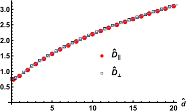
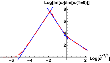
Figure 4: On the left panel we compare the numerical results for the reduced in-plane and off-plane diffusion constants $\hat{D}_{\parallel}$ and $\hat{D}_{\perp}$ (discrete points) and the analytic results (4.82) and (4.96) (continuous curve). On the right panel, we plot the imaginary part of the lowest in-plane excitation mode, keeping $\hat{k}_{\parallel}/\hat{d}^{3/8}=0.01$, so that both the density and the wavevector are kept fixed and only the temperature varies. The red points are numerical results and the line segments have slopes $0$, $7/3$, -$7/3$, -$1$ from left to right. The latter two slopes correspond to the low and high temperature behavior of the diffusion constant (see (4.87) and (4.84)).

We have solved (4.20) numerically and checked that, indeed, for high enough temperature the diffusive mode is the dominant one. This numerical analysis allows us to extract the diffusion constant and to compare the result with the analytic formula (4.82). This comparison is performed in Figure 4, where we see that the agreement between (4.82) and the numerical results is very good.

When the temperature is low enough, the zero sound mode is the dominant one and the system enters a collisionless regime. This collisionless/hydrodynamic crossover is illustrated in Figure 4, where we notice that the zero sound persists at $T\not=0$ if $T$ is small enough. When $T$ is increased, the imaginary part of the zero sound grows as $T^{{7\over 3}}$ until the crossover to the hydrodynamic diffusive regime takes place. The frequency $\omega_{cr}$ and momentum $k^{\parallel}_{cr}$ at which this transition occurs depend on the temperature and chemical potential. Our numerical analysis has allowed us to determine that $\omega_{cr}$ and $k^{\parallel}_{cr}$ scale with $T$ and $\mu$ as:

$$\omega_{cr}\sim{T^{{7\over 3}}\over\mu}\,\,,\qquad\qquad k^{\parallel}_{cr}\sim{T^{{7\over 3}}\over\mu}\,\,.$$ (4.88)

In Figure 5 we display typical dispersion relations of several excitation modes for the in-plane case. The off-plane dispersion relations are qualitatively the same. We notice that the zero sound dispersion saturates at high frequencies. This is due to interactions between complex modes, as is clear from the figure. It would be tempting to identify this in-plane zero sound mode with a surface plasmon polariton, whose dispersion relation has close resemblance. However, we cannot clearly separate the underlying physics and associate the saturation directly with surface phenomena due to the following observation: We found out that for any flavor D$q$-brane configuration that we have tested, the zero sound saturates if one reaches high enough frequency. This in itself is remarkable and had gone unnoticed in all the previous works in this field. It would be very interesting to understand why this happens and in particular discern if this phenomenon is due to non-linearities of the DBI action.

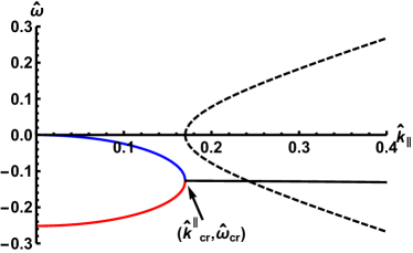
Figure 5: We display the typical dispersion relations for the in-plane case (off-plane is qualitatively the same) at $\hat{d}=10$. The solid curves denote imaginary parts while dashed curves are real parts of the modes. On the right panel we extend the range of $\hat{k}_{\parallel}$ and notice that the zero sound collides with complex modes, eventually leading to saturation.

4.3.2 Off-plane diffusion

Let us now study the off-plane fluctuation equation (4.44) in the diffusive regime. We first expand the coefficients of $E^{\prime}$ and $E$ near the horizon as:

$$\partial_{r}\log\Bigg{[}{e^{{3\phi\over 2}}\,\big{(}H+d^{2}\big{)}^{{3\over 2}}\,B\over(\omega^{2}-k_{\perp}^{2}\,B\,e^{2\phi})\,H\,+\,\omega^{2}\,d^{2}}\Bigg{]} = {1\over r-r_{h}}\,+\,\tilde{c}_{1}+\ldots$$

$${h\over B^{2}}\,{(\omega^{2}-k_{\perp}^{2}\,B\,e^{2\phi})\,H\,+\,\omega^{2}\,d^{2}\over H+d^{2}} = {\tilde{A}\over(r-r_{h})^{2}}\,+\,{\tilde{c}_{2}\over r-r_{h}}+\ldots\ ,$$ (4.89)

where $\tilde{A}$, $\tilde{c}_{1}$, and $\tilde{c}_{2}$ are given by:

$$\tilde{A} = {9\,R^{4}\over 100\,r_{h}^{2}}\,\omega^{2}$$

$$\tilde{c}_{1} = {10\over 3\alpha}\,\,{r_{h}^{{17\over 3}}\over d^{\,2}+\alpha\,r_{h}^{{16\over 3}}}\,\,{k^{2}\over\omega^{2}}\,+{3\over 2r_{h}}\,-\,{8\over 3}\,{d^{\,2}\over r_{h}\,\Big{(}d^{\,2}+\alpha\,r_{h}^{{16\over 3}}\Big{)}}$$

$$\tilde{c}_{2} = -{3\,\,R^{4}\over 10\alpha}\,{r_{h}^{{11\over 3}}\over d^{\,2}+\alpha\,r_{h}^{{16\over 3}}}\,k^{2}+{3\,R^{4}\over 100\,r_{h}^{3}}\,\omega^{2}\ .$$ (4.90)

Following the same procedure as in the in-plane case, we next expand $E(r)$ at low frequency and write $E(r)$ near the horizon as in (4.69), where now $\beta$ is given at leading order by:

$$\beta\,=\,i\,{k_{\perp}^{2}\over\omega}\,{R^{2}\,r_{h}^{{14\over 3}}\over\alpha\,\Big{(}d^{\,2}+\alpha\,r_{h}^{{16\over 3}}\Big{)}}\ .$$ (4.91)

Taking the limits in the opposite order, we arrive exactly at (4.70). Thus, we can expand $E(r)$ as in (4.72) with ${\cal I}$ being the integral written in (4.73). The constant $c_{E}$ can be obtained from the consistency of both expansions. This procedure yields

$$c_{E}=-i\,{k_{\perp}^{2}\over\omega}\,{R^{2}\over\alpha^{2}\,r_{h}}\,\Big{(}r_{h}^{{16\over 3}}\,+\,{d^{\,2}\over\alpha}\Big{)}^{{1\over 2}}\,E_{nh}\ ,$$ (4.92)

and, by again imposing Dirichlet boundary conditions at the UV we get the diffusion dispersion relation $\omega\,=\,-i\,D_{\perp}\,k_{\perp}^{2}+\ldots$, where $D_{\perp}$ is given by:

$$D_{\perp}={3\,r_{h}^{{1\over 3}}\,R^{2}\over 4\,\alpha^{2}}\,\Big{(}1\,+\,{d^{\,2}\over\alpha\,r_{h}^{{16\over 3}}}\Big{)}^{{1\over 2}}F\Big{(}{1\over 4}\,,\,{3\over 2}\,;{5\over 4}\,;\,-{d^{\,2}\over\alpha\,r_{h}^{{16\over 3}}}\Big{)}\ .$$ (4.93)

Let us now reintroduce reduced quantities $\hat{d}$, $\hat{\omega}$, and $\hat{k}_{\perp}$ which allow to absorb $R$, $r_{h}$, and $\alpha$ in (4.44). Due to different scaling in the off-plane direction one needs to be a bit more careful with the momentum. The $\hat{d}$ and $\hat{\omega}$ are defined as in (4.79), whereas $\hat{k}_{\perp}$ must be defined as:

$$\hat{k}_{\perp}\,=\,{R^{2}\over\alpha\,r_{h}^{{1\over 3}}}\,k_{\perp}\ .$$ (4.94)

Using these definitions the dispersion relation for the off-plane diffusion can be written as $\hat{\omega}\,=\,-i\,\hat{D}_{\perp}\,\hat{k}_{\perp}^{2}+\ldots$, where $\hat{D}_{\perp}$ is related to $D_{\perp}$ as:

$$\hat{D}_{\perp}\,=\,{\alpha^{2}\over r_{h}^{{1\over 3}}\,R^{2}}\,D_{\perp}\,=\,\Big{(}{5\over 6\pi}\Big{)}^{{1\over 3}}\,{\alpha^{2}\over R^{{8\over 3}}}\,{D_{\perp}\over T^{{1\over 3}}}\,\,.$$ (4.95)

Moreover, from the expression of $D_{\perp}$ in (4.93) we get that $\hat{D}_{\perp}$ is given by:

$$\hat{D}_{\perp}\,=\,{3\over 4}\big{(}1+\hat{d}^{\,2}\big{)}^{{1\over 2}}\,F\Big{(}{1\over 4}\,,\,{3\over 2}\,;{5\over 4}\,;\,-\hat{d}^{\,2}\Big{)}\,\,,$$ (4.96)

which means that $\hat{D}_{\perp}=\hat{D}_{\parallel}$. The fact that the reduced, non-physical, in-plane and off-plane diffusion constants can be made equal by a temperature-dependent rescaling is a reflection of the scaling symmetry of the background metric. However, we should emphasize that the physical diffusion constants $D_{\perp}$ and $D_{\parallel}$ behave rather differently due to the different scalings used to define the corresponding hatted quantities. For example, at high temperature $\hat{D}_{\perp}=\hat{D}_{\parallel}\approx{3\over 4}$ and thus:

$$D_{\perp}={3\over 4}\Big{(}{6\pi\over 5}\Big{)}^{{1\over 3}}\,{R^{{8\over 3}}\over\alpha^{2}}\,T^{{1\over 3}}\,\,,\qquad\qquad(T\rightarrow\infty)\,\,,$$ (4.97)

which means that, contrary to $D_{\parallel}$, the off-plane diffusion constant grows as $T^{{1\over 3}}$ for large $T$. Moreover, at low temperature, $\hat{D}_{\perp}\,\sim\,\hat{d}^{{1\over 2}}\sim T^{-{4\over 3}}$ and, since $D_{\perp}\sim T^{{1\over 3}}\,\hat{D}_{\perp}$, we have:

$$D_{\perp}\sim T^{-1}\,\,.\qquad\qquad(T\rightarrow 0)\,\,.$$ (4.98)

5 Discussion

Holography offers a possibility to investigate various phases of dense matter in the strong coupling regime. Intense effort has been put to study inhomogeneous phases, starting with the early works of [102, 103] with the first explicit example [80] showing striped phases for fundamental matter realized with defect flavor D7’-branes in $AdS_{5}\times S^{5}$ spacetime [66]. The construction and analysis of such modulated ground states has led to increasingly demanding numerics [104, 105, 106] due to the highly non-linear DBI action.

Another important merit of holographic techniques is to yield useful toy models that keep computations simple. The D3-D5 geometry [29] has provided us with a powerful framework to study anisotropic media; in the present paper, we probe this medium with fundamental matter and explore both the thermodynamics and the excitation spectra along and across the anisotropic direction. We believe that our work sets the standard and sparks many other investigations in the future. One particularly interesting case is in the context of the astrophysics of compact objects where anisotropy seems to offer clues regarding the “universal relations” for neutron stars [111] and the already established holographic modeling of isotropic matter [112, 113, 114, 70, 115, 116, 117].

While the D3-D5 geometry enables a multitude of investigations of anisotropic matter, it is not at all perfect. The real life anisotropic systems in laboratories consist of a finite number of layers of perhaps different materials with finite separation. The D3-D5 system is an idealization: The anisotropic direction spans an infinite range and the separation between the layers is strictly vanishing. Interestingly, contrary to common beliefs, relaxing these approximations in a controlled fashion may not be a major hurdle and can be obtained by a judicious selection of the smearing form for the D5-branes. Reaching this milestone would be very rewarding and will teach us further lessons on surface phenomena. In particular, it would allow us to dissect the issues of the surface plasmon left open in this paper. Besides, the shear-viscosity over entropy density bound [118, 119] is known to be affected by anisotropy [120, 121, 122, 123, 124, 125]; it would be interesting to consider the status of the bound in the presence of a further scale introduced by a finite inter-layer spacing. Furthermore, a finite-spacing would break the translations along the orthogonal direction to the layers.

Acknowledgements

We would like to thank Daniel Areán, Carlos Hoyos, and Javier Tarrío for relevant and interesting discussions. The research of U. G. and M. T. has been funded by the Swedish Research Council. The research of N. J. has been supported in part by the Academy of Finland grant no. 1322307. The research of D. M. and A. V. R. has been funded by the Spanish grants FPA2014-52218-P and FPA2017-84436-P by Xunta de Galicia (ED431C-2017/07), by FEDER, and by the María de Maeztu Unit of Excellence MDM-2016-0692.

Appendix A Kappa symmetry

Let us verify that the embeddings we found in Section 3.1 are supersymmetric. We will work in the following vielbein basis for the metric presented in Section 2 for $B=1$:

$$E^{x^{\mu}}\,=\,h^{-{1\over 4}}\,dx^{\mu}\,\,,\qquad\qquad(\mu=0,1,2),\qquad\qquad E^{x^{3}}\,=\,h^{-{1\over 4}}\,e^{-\phi}\,dx^{3}\,\,,$$

$$E^{r}\,=\,h^{{1\over 4}}\,dr\,\,,\qquad\qquad E^{i}\,=\,{1\over 2}\,h^{{1\over 4}}\,e^{g}\,\cos\chi\,\,\omega^{i}\,\,,\qquad\qquad(i=1,2)\,\,,$$

$$E^{3}\,=\,{1\over 2}\,h^{{1\over 4}}\,e^{g}\,\cos\chi\,\sin\chi\,\omega^{3}\,\,,\qquad\qquad E^{4}\,=\,h^{{1\over 4}}\,e^{g}\,d\chi\,\,,$$

$$E^{5}\,=\,h^{{1\over 4}}\,e^{f}\,\big{(}d\tau+{1\over 2}\cos^{2}\chi\,\,\omega^{3}\big{)}\,\,,$$ (A.1)

where the warp factor $h$ is the function written in (2.4) and $g$ and $f$ are given by:

$$e^{g}\,=\,{r\over\sqrt{b}}\,\,,\qquad\qquad e^{f}\,=\,{r\over b}\,\,.$$ (A.2)

We will write the SU(2) left-invariant one-forms $\omega^{1}$, $\omega^{2}$, and $\omega^{3}$ in terms of three angles $(\theta,\varphi,\psi)$ as follows:

$$\omega^{1}\,=\,\cos\psi\,d\theta\,+\,\sin\psi\,\sin\theta\,d\varphi$$

$$\omega^{2}\,=\,\sin\psi\,d\theta\,-\,\cos\psi\,\sin\theta\,d\varphi$$

$$\omega^{3}\,=\,d\psi\,+\,\cos\theta\,d\varphi\,\,,$$ (A.3)

where $0\leq\theta\leq\pi$, $0\leq\varphi<2\pi$, and $0\leq\psi<4\pi$.

The supersymmetric embeddings of the D7-brane are those that satisfy the kappa symmetry condition:

$$\Gamma_{\kappa}\,\epsilon\,=\,\pm\epsilon\,\,,$$ (A.4)

where $\epsilon$ is a Killing spinor of the background. For a D7-brane without any worldvolume gauge field, the matrix $\Gamma_{\kappa}$ is given by:

$$\Gamma_{\kappa}\,=\,{1\over 8!\sqrt{-g_{8}}}\,\,\epsilon^{\alpha_{1}\,\cdots\,\alpha_{8}}\,i\sigma_{2}\,\gamma_{\alpha_{1}\cdots\alpha_{8}}\,\,,$$ (A.5)

where $\gamma_{\alpha_{1}\cdots\alpha_{8}}$ is the antisymmetrized product of induced Dirac matrices and $\sigma_{2}$ is the Pauli matrix. We will take the following set of worldvolume coordinates:

$$\xi^{\alpha}\,=\,(x^{0},x^{1},x^{2},x^{3},r,\theta,\psi,\varphi)\,\,,$$ (A.6)

and the embedding will be determined by two embedding equations of the type:

$$\tau\,=\,{\rm constant}\,\,,\qquad\qquad\chi\,=\,\chi(r)\,\,.$$ (A.7)

The kappa symmetry matrix for this ansatz is:

$$\Gamma_{\kappa}\,=\,{i\sigma_{2}\over\sqrt{-g_{8}}}\,\,\gamma_{x^{0}x^{1}x^{2}x^{3}r\theta\psi\varphi}\,\,.$$ (A.8)

To obtain the induced $\gamma$-matrices, let us write the vielbein one-forms (A.1) in a coordinate basis as:

$$E^{\underline{M}}\,=\,{\cal E}^{\underline{M}}_{N}\,dX^{N}\,\,.$$ (A.9)

Then, the $\gamma$’s are:

$$\gamma_{\alpha}\,=\,\partial_{\alpha}X^{N}\,{\cal E}^{\underline{M}}_{N}\,\Gamma_{\underline{M}}\,\,,$$ (A.10)

where the $\Gamma$’s are flat constant matrices for the vielbein (A.1). Specifically, the induced $\gamma$-matrices on the worldvolume for our configuration are:

$$\gamma_{x^{\mu}}\,=\,h^{-{1\over 4}}\,\Gamma_{x^{\mu}}\,\,,\qquad\qquad(\mu=0,1,2)\,\,,$$

$$\gamma_{x^{3}}\,=\,h^{-{1\over 4}}\,e^{-\phi}\,\Gamma_{x^{3}}\,,\,\qquad\qquad\gamma_{r}\,=\,h^{{1\over 4}}\,\big{[}\Gamma_{r}\,+\,e^{g}\,\chi^{\prime}\,\Gamma_{4}\big{]}\,\,,$$

$$\gamma_{\theta}\,=\,{h^{{1\over 4}}\over 2}\,\cos\chi\,e^{g}\big{[}\cos\psi\Gamma_{1}\,+\,\sin\psi\Gamma_{2}\big{]}\,\,,\quad\gamma_{\psi}\,=\,{h^{{1\over 4}}\over 2}\,\cos\chi\,\big{[}\sin\chi\,e^{g}\,\Gamma_{3}\,+\,\cos\chi\,e^{f}\,\Gamma_{5}\big{]}\,\,,$$

$$\gamma_{\varphi}={h^{{1\over 4}}\over 2}\cos\chi\big{[}\sin\psi\sin\theta e^{g}\Gamma_{1}-\cos\psi\sin\theta e^{g}\Gamma_{2}+\sin\chi\cos\theta e^{g}\Gamma_{3}+\cos\chi\,\cos\theta e^{f}\Gamma_{5}\big{]}\,\,.\qquad$$ (A.11)

Clearly, we can factorize the antisymmetrized product in (A.8) as:

$$\gamma_{x^{0}x^{1}x^{2}x^{3}r\theta\psi\varphi}\,=\,\gamma_{x^{0}x^{1}x^{2}x^{3}}\,\gamma_{r\theta\psi\varphi}\,\,,$$ (A.12)

where the first factor is:

$$\gamma_{x^{0}x^{1}x^{2}x^{3}}\,=\,h^{-1}\,e^{-\phi}\,\Gamma_{x^{0}x^{1}x^{2}x^{3}}\,\,.$$ (A.13)

The second factor can be written as:

$$\gamma_{r\theta\psi\varphi}\,=\,{h\over 8}\,e^{2g}\,\cos^{3}\chi\,\sin\theta\,\Gamma_{12}\,\big{[}\,c_{1}\,\Gamma_{r3}\,+\,c_{2}\,\Gamma_{r5}\,+\,c_{3}\,\Gamma_{34}\,+\,c_{4}\,\Gamma_{45}\big{]}\,,$$ (A.14)

where the $c_{i}$ coefficients are given by:

$$c_{1}\,=\,e^{g}\,\sin\chi\,\,,\qquad\qquad\qquad c_{2}\,=\,e^{f}\,\cos\chi\,\,,$$

$$c_{3}\,=\,-e^{2g}\,\sin\chi\,\chi^{\prime}\,\,,\qquad\qquad c_{4}\,=\,e^{g+f}\cos\chi\,\chi^{\prime}\,\,.$$ (A.15)

Putting everything together, we can write $\Gamma_{\kappa}$ as:

$$\Gamma_{\kappa}\,=\,{e^{-\phi+2g}\over 8\,\sqrt{-g_{8}}}\,\cos^{3}\chi\,\sin\theta\,(i\sigma_{2})\,\Gamma_{x^{0}x^{1}x^{2}x^{3}}\,\Gamma_{12}\,\big{[}c_{1}\,\Gamma_{r3}\,+\,c_{2}\,\Gamma_{r5}\,+\,c_{3}\,\Gamma_{34}\,+\,c_{4}\,\Gamma_{45}\big{]}\,\,.$$ (A.16)

It was proven in [29] that the Killing spinor of the background can be written as:

$$\epsilon\,=\,h^{-{1\over 8}}\,e^{{3\over 2}\,\Gamma_{12}\,\tau}\,\,\eta\,\,,$$ (A.17)

where $\eta$ is a doublet of constant Majorana-Weyl spinor satisfying the following projection conditions:

$$\Gamma_{x^{0}\,x^{1}\,x^{2}\,x^{3}}\,(i\sigma_{2})\,\eta\,=\,\eta$$

$$\Gamma_{rx^{3}14}\,\sigma_{1}\,\eta\,=\,\eta$$

$$\Gamma_{12}\,\eta\,=\,\Gamma_{34}\,\eta\,=\,\Gamma_{r5}\,\eta\,=\,i\sigma_{2}\,\eta\,\,.$$ (A.18)

As $\Gamma_{12}$ commutes with the products of matrices of the rhs of (A.16), we can rewrite the kappa symmetry condition (A.4) as:

$$\Gamma_{\kappa}\,\eta\,=\,\pm\eta\,\,.$$ (A.19)

Moreover, from the last equation in (A.18) one can easily demonstrate that:

$$\Gamma_{45}\,\eta\,=\,\Gamma_{r3}\,\eta\,\,.$$ (A.20)

Thus, $\Gamma_{\kappa}$ acting on $\eta$ can be written as:

$$\Gamma_{\kappa}\,\eta\,=\,{e^{-\phi+2g}\over 8\,\sqrt{-g_{8}}}\,\cos^{3}\chi\,\sin\theta\,\big{[}(c_{1}+c_{4})\Gamma_{45}\,+\,(c_{2}+c_{3})i\sigma_{2}\big{]}(i\sigma_{2})\,\Gamma_{x^{0}x^{1}x^{2}x^{3}}\,\Gamma_{12}\,\eta\,\,.$$ (A.21)

Moreover, since from (A.18) we have:

$$(i\sigma_{2})\,\Gamma_{x^{0}x^{1}x^{2}x^{3}}\,\Gamma_{12}\,\eta\,=\,(i\sigma_{2})\,\eta\,\,,$$ (A.22)

we can write $\Gamma_{\kappa}\eta$ simply as:

$$\Gamma_{\kappa}\,\eta\,=\,{e^{-\phi+2g}\over 8\,\sqrt{-g_{8}}}\,\cos^{3}\chi\,\sin\theta\,\big{[}-(c_{2}+c_{3})\,+\,(c_{1}+c_{4})\,\Gamma_{45}\,(i\sigma_{2})\big{]}\,\eta\,\,.$$ (A.23)

According to (A.19), we are looking for embeddings such that $\Gamma_{k}$ acts on $\eta$ as plus/minus the identity. Inspecting the rhs of (A.23) we notice that the last two terms act on $\eta$ as a non-trivial matrix. Therefore, we should require that the coefficient of these terms is zero, namely:

$$c_{1}+c_{4}=0\,\,,$$ (A.24)

which is the BPS equation for the embedding. Taking into account the values of $c_{1}$ and $c_{4}$ written in (A.15), we can recast (A.24) as the following first-order differential equation:

$$e^{f}\,\chi^{\prime}\,=\,-\tan\chi\,\,.$$ (A.25)

Using the value of $e^{f}$ displayed in (A.2), we can rewrite this BPS equation as:

$${r\over b}\,{d\chi\over dr}\,=\,-\tan\chi\,\,,$$ (A.26)

which is the same as (3.7). Notice that the general solution of (A.26) is indeed (3.1). To finish with the proof of kappa symmetry, let us compute the terms of $\Gamma_{\kappa}\,\eta$ which are proportional to the unit matrix. One can readily prove from (2.16) and (A.15) that, when the BPS condition (A.26) holds, we have:

$$\sqrt{-g_{8}}\big{|}_{BPS} = {r^{3}\,e^{-\phi}\,\cos^{2}\chi\,\sin\theta\over 8\,b^{2}}\,\big{[}\cos^{2}\chi+b\,\sin^{2}\chi\big{]}$$

$$(c_{2}+c_{3})\big{|}_{BPS} = {r\over b\,\cos\chi}\,\big{[}\cos^{2}\chi+b\,\sin^{2}\chi\big{]}\ .$$ (A.27)

From these two equations we get:

$$\sqrt{-g_{8}}\big{|}_{BPS}\,=\,{e^{2g-\phi}\,\cos^{3}\chi\,\sin\theta\over 8}\,(c_{2}+c_{3})\big{|}_{BPS}\,\,,$$ (A.28)

and, as a consequence,

$$\Gamma_{\kappa}\,\eta\,=\,-\eta\,\,.$$ (A.29)

Appendix B The dictionary

The bare quark mass $m_{q}$ is obtained from the Nambu-Goto action of a fundamental string hanging from the boundary to the horizon. We will obtain $m_{q}$ as the limit of the constituent quark mass $M_{c}$, which contains the effects of the thermal screening of the quarks and is also obtained from the Nambu-Goto action. Let us consider a fundamental string extended in $t$, $P$ at constant $\rho=0$. The induced metric is:

$$ds_{2}^{2}\,=\,-{r_{h}^{2}\over 2^{{6\over 5}}\,R^{2}}\,P^{{9\over 4}}\,(1+P^{-{15\over 4}})^{-{4\over 5}}\,(1-P^{-{15\over 4}})^{2}\,dt^{2}\,+\,\Big{(}{9\over 8}\Big{)}^{2}\,R^{2}\,{dP^{2}\over P^{2}}\,\,,$$ (B.1)

whose determinant is:

$$\sqrt{-\det g_{2}}\,=\,{9\over 8}\,{r_{h}\over 2^{{3\over 5}}}\,P^{{1\over 8}}\,{1-P^{-{15\over 4}}\over(1+P^{-{15\over 4}})^{{2\over 5}}}\,\,.$$ (B.2)

The constituent quark mass $M_{c}$ is minus the action per unit of time of the Nambu-Goto action:

$$M_{c}\,=\,{1\over 2\pi}\,\int_{1}^{P_{0}}\,e^{{\phi\over 2}}\,\sqrt{-\det g_{2}}\,\,dP\,\,,$$ (B.3)

where the $e^{{\phi\over 2}}$ factor is due the fact that our metric is written in Einstein frame ($g_{string}=e^{{\phi\over 2}}\,g_{Einstein}$). When $\rho=0$, we have:

$$e^{{\phi\over 2}}\,=\,\Big{(}{3\over 4\,Q_{f}}\Big{)}^{{1\over 3}}\,{r_{h}^{{1\over 3}}\over 2^{{1\over 5}}}\,\,P^{{3\over 8}}\,(1+P^{-{15\over 4}})^{{1\over 5}}\,\,.$$ (B.4)

Plugging this into (B.3), we get:

$$M_{c}\,=\,{9\over 16\,\pi}\,\,\Big{(}{3\over 4\,Q_{f}}\Big{)}^{{1\over 3}}\,{r_{h}^{{4\over 3}}\over 2^{{4\over 5}}}\,J(P_{0})\ ,$$ (B.5)

where $J(P_{0})$ is defined as the following integral:

$$J(P_{0})\equiv\int_{1}^{P_{0}}\,dP\,{P^{{1\over 2}}(1-P^{-{15\over 4}})\over(1+P^{-{15\over 4}})^{{1\over 5}}}\,\,.$$ (B.6)

This integral can be obtained in analytic form and is given by:

$$J(P_{0})\,=\,{2\over 3}\,\Big{[}P_{0}^{{3\over 2}}\Big{(}1+{1\over P_{0}^{{15\over 4}}}\Big{)}^{{4\over 5}}\,-\,2^{{4\over 5}}\Big{]}\,\,.$$ (B.7)

In order to get the bare quark mass $m_{q}$, let us write $P_{0}=m$ and consider the limit $m\rightarrow\infty$, where $M_{c}$ equals $m_{q}$. We get:

$$m_{q}\,=\,{3\over 8\pi\,2^{{4\over 5}}}\,\Big{(}{3\over 4\,Q_{f}}\Big{)}^{{1\over 3}}\,r_{h}^{{4\over 3}}\,m^{{3\over 2}}\,\,.$$ (B.8)

Notice that, for fixed $m_{q}$ the mass parameter $m$ depends on the temperature as $m\approx T^{-{8\over 9}}=T^{-b}$.

The condensate $\langle{\cal O}_{m}\rangle$ is obtained by computing the derivative of the free energy $F$ with respect to the bare quark mass $m_{q}$:

$$\langle{\cal O}_{m}\rangle\,=\,{\partial F\over\partial m_{q}}={2\over 3}{m\over m_{q}}{\partial F\over\partial m}\ .$$ (B.9)

The free energy $F$ can be written as:

$$F\,=\,{\cal N}\,\big{(}{\cal I}_{bulk}+{\cal I}_{bdy}\big{)}\,\,,$$ (B.10)

where ${\cal N}$ is written in (3.29), ${\cal I}_{bulk}$ is the integral (3.30) evaluated on-shell and ${\cal I}_{bay}$ is given in (3.40). Since the normalization factor ${\cal N}$ does not depend on the mass parameter $m$, we have:

$${\partial F\over\partial m}\,=\,{\cal N}\,\Big{(}{\partial{\cal\cal I}_{bulk}\over\partial m}\,+\,{\partial{\cal\cal I}_{bdy}\over\partial m}\Big{)}$$ (B.11)

In order to compute its derivative with respect to the mass parameter $m$, let us write the bulk action as:

$${\cal\cal I}_{bulk}\,=\,\int_{u_{min}}^{u_{max}}\,du\,{\cal J}(u,\eta,\dot{\eta})\,\,,$$ (B.12)

where ${\cal J}$ is given by:

$${\cal J}\,=\,u^{{7\over 2}}\,f\,\tilde{f}^{{7\over 5}}\,(1-\eta^{2})\,\sqrt{1-{\eta^{2}\over 9}}\,\sqrt{1-\eta^{2}+{8u^{2}\over 9}\,\dot{\eta}^{2}}\,\,.$$ (B.13)

Then:

$${\partial{\cal\cal I}_{bulk}\over\partial m}\,=\,\int_{u_{min}}^{u_{max}}\,du\Big{[}{\partial{\cal J}\over\partial\dot{\eta}}\,{d\over du}\Big{(}{\partial\eta\over\partial m}\Big{)}\,+\,{\partial{\cal J}\over\partial\eta}\,{\partial\eta\over\partial m}\,\Big{]}\,\,.$$ (B.14)

Taking into account that the on-shell action satisfies the Euler-Lagrange equation ${\partial{\cal J}\over\partial\eta}\,=\,{d\over du}\,\Big{(}{\partial{\cal J}\over\partial\dot{\eta}}\Big{)}$, we can integrate this equation and write:

$${\partial{\cal\cal I}_{bulk}\over\partial m}\,=\,{\partial{\cal J}\over\partial\dot{\eta}}\,{\partial\eta\over\partial m}\Big{|}_{u_{min}}^{u_{max}}\,\,.$$ (B.15)

The momentum appearing on the right-hand side of this equation is:

$${\partial{\cal J}\over\partial\dot{\eta}}\,=\,{8\over 9}\,u^{{11\over 2}}\,f\,\tilde{f}^{{7\over 5}}\,{(1-\eta^{2})\,\sqrt{1-{\eta^{2}\over 9}}\over\sqrt{1-\eta^{2}+{8u^{2}\over 9}\,\dot{\eta}^{2}}}\,\,\dot{\eta}\,\,.$$ (B.16)

Let us consider a black hole embedding, in which $u_{min}=1$. In this case the momentum (B.16) vanishes at the lower value in (B.15) and the only non-vanishing contribution comes from the upper limit $u_{\max}\rightarrow\infty$. To evaluate this contribution we use the asymptotic UV expansion (3.31), as well as:

$$\dot{\eta}\,=\,-{m\over u^{2}}\,-\,{7\over 2}\,{c\over u^{{9\over 2}}}\,+\,\ldots\,\,,\qquad\qquad{\partial\eta\over\partial m}\,=\,{1\over u}\,+\,{1\over u^{{7\over 2}}}\,{\partial c\over\partial m}\,+\,\ldots\,\,.$$ (B.17)

We get:

$${\partial{\cal\cal I}_{bulk}\over\partial m}\,=\,{\partial{\cal J}\over\partial\dot{\eta}}\,{\partial\eta\over\partial m}\Big{|}_{u_{max}}\,=\,{8\over 9}\,m\,u_{max}^{{1\over 2}}(m^{2}-u_{max}^{2})\,-\,{28\over 9}\,c\,-\,{8\over 9}\,m\,{\partial c\over\partial m}\,\,,$$ (B.18)

where we have only included terms that are non-vanishing when $u_{max}\rightarrow\infty$. Moreover, by computing the derivative with respect to $m$ of the explicit expression of ${\cal\cal I}_{bdy}$ written in (3.40), we obtain:

$${\partial{\cal\cal I}_{bdy}\over\partial m}\,=\,-{8\over 9}\,m\,u_{max}^{{1\over 2}}(m^{2}-u_{max}^{2})\,+\,{8\over 9}\,c\,+\,{8\over 9}\,m\,{\partial c\over\partial m}\,\,.$$ (B.19)

Adding (B.18) and (B.19) we notice that the result is finite when $u_{max}\rightarrow\infty$ and given by

$${\partial F\over\partial m}\,=\,-{20\over 9}\,{\cal N}\,c\,\,.$$ (B.20)

Notice also that the terms containing $\partial c/\partial m$ vanish and the VEV $\langle{\cal O}_{m}\rangle$ is proportional to $c$, as expected:

$$\langle{\cal O}_{m}\rangle\,=\,-{40\over 27}\,{m\,{\cal N}\over m_{q}}\,c\,\,.$$ (B.21)

Appendix C Critical embeddings

In this appendix we perform an analysis of critical embeddings, at zero density and non-zero temperature, of the probe D7-brane along the lines of [65, 56]. In these configurations the D7-brane touches the horizon near $\chi=\pi/2$. It is then useful to define the following new coordinates $(y,z)$ as

$$\chi=\frac{\pi}{2}-\frac{\sqrt{b}}{R}\,y\ ,\qquad r=r_{h}+Cz^{\alpha}\ ,$$ (C.1)

to zoom on the vicinity of the contact point. In (C.1) $C$ and $\alpha$ are constants to be determined in order to cast the induced metric into a Rindler form. In the new coordinates (C.1), the emblackening factor $B(r)$ near the horizon reads

$$B(r)=1-\left(\frac{r_{h}}{r}\right)^{\frac{10}{3}}=\frac{10}{3}\frac{C}{r_{h}}z^{\alpha}+\ldots\ .$$ (C.2)

Choosing

$$\alpha=2\ ,\qquad C=\frac{5}{6}\frac{r_{h}}{R^{2}}=\pi T\ ,$$ (C.3)

where $T$ is the temperature defined in (6.111), the radial and temporal pieces of the induced metric take the desired Rindler form, namely

$$\left.ds^{2}\right|_{(t,z)}=-(2\pi T)^{2}z^{2}dt^{2}+dz^{2}\ .$$ (C.4)

In terms of the $z$ and $y$ coordinates, the metric in the vicinity of the horizon, at leading order, becomes

$$\begin{split}ds^{2}_{8}=&-(2\pi T)^{2}z^{2}dt^{2}+\frac{r_{h}^{2}}{R^{2}}\left[(dx^{1})^{2}+(dx^{2})^{2}+e^{-2\phi}(dx^{3})^{2}\right]\\ &\qquad+dz^{2}+dy^{2}+\frac{y^{2}}{4}\left[(\omega_{1})^{2}+(\omega_{2})^{2}+(\omega_{3})^{2}\right]\,+\,\ldots\,\,,\end{split}$$ (C.5)

where the ellipsis represents terms that do not contribute to the embedding of the probe. Describing the D7 embedding with the parametrization $y=y(z)$, one has $dz^{2}+dy^{2}=(1+\dot{y}^{2})dz^{2}$, where the dot denotes derivation with respect to $z$. Substituting into the metric (C.5), one obtains the associated DBI Lagrangian density

$${\cal L}_{\text{DBI}}\propto\,z\,y^{3}\,\sqrt{1+\dot{y}^{2}}\ .$$ (C.6)

The equation of motion descending from (C.6) is

$$zy\ddot{y}+(y\dot{y}-3z)(1+\dot{y}^{2})=0\ .$$ (C.7)

The Lagrangian density (C.6) and the associated equation of motion (C.7) correspond to the case $n=3$ in the generic analysis performed in [65], according to the fact that three internal directions wrapped by the D7-brane collapse in the critical embedding at $y=0$. More generically, the parametrization $y=y(z)$ is suitable to describe near-to-critical black hole embeddings where the D7-brane intersects the horizon at an angle

$$\chi_{h}=\frac{\pi}{2}-\frac{\sqrt{b}}{R}\,y_{h}\ ,$$ (C.8)

according to (C.1) where $y_{h}=y(z=0)$. More precisely, the equation of motion (C.7) must be solved imposing the boundary conditions

$$y(z=0)=y_{h}\ .$$ (C.9)

By consistency

$$\dot{y}(z=0)=0\ ,$$ (C.10)

which can be seen solving the equation order by order.

To study the near-to-critical Minkowski embeddings instead, one has to parameterize the embeddings as $z=z(y)$, where $z_{h}=z(y=0)$ represents the IR radial distance of the D7-brane from the horizon. From (C.5) one gets the DBI Lagrangian

$${\cal L}_{\text{DBI}}\propto\,z\,y^{3}\,\sqrt{1+z^{\prime 2}}\ ,$$ (C.11)

where the prime denotes differentiation with respect to $y$. The associated equation of motion is

$$yzz^{\prime\prime}+(3zz^{\prime}-y)(1+z^{\prime 2})=0\ ,$$ (C.12)

to be solved imposing the boundary conditions

$$z(y=0)=z_{h}\ ,$$ (C.13)

that implies

$$z^{\prime}(y=0)=0\ .$$ (C.14)

The critical solution

$$y=\sqrt{3}z\ ,$$ (C.15)

solves both (C.7) and (C.12) with boundary conditions

$$y_{h}=z_{h}=0\ .$$ (C.16)

The critical solution (C.15) can be seen as a limiting case of both near-critical black hole and Minkowski embeddings. The limit involves appropriate scaling of $y_{h}$ and $z_{h}$ in the pinching direction, $z$ and $y$, respectively.

Let us now write the critical solution in terms of the isotropic variable $u$ defined in (3.10), rewritten as

$$u^{\frac{5}{3b}}=\left(\frac{r}{r_{h}}\right)^{\frac{5}{3}}\left(1+\sqrt{B(r)}\right)=\left(\frac{r}{r_{h}}\right)^{\frac{5}{3}}\left(1+\sqrt{1-\left(\frac{r_{h}}{r}\right)^{\frac{10}{3}}}\right)\ .$$ (C.17)

Recalling the definition of the coordinate $z$ in (C.1) and using (C.3), near the horizon one has

$$u^{\frac{5}{3b}}=1+\sqrt{\frac{10}{3}\frac{\pi T}{r_{h}}}\ z+\ldots=1+\frac{5}{3R}\ z+\ldots\ \rightarrow\ u=1+\frac{b}{R}\,z+\ldots\ .$$ (C.18)

Adopting the Cartesian-like coordinates (3.55) and recalling (C.1), in the near-horizon region one has

$$P\sim u\sim 1+\frac{b}{R}\,z\ ,\qquad\rho\sim\frac{\sqrt{b}}{R}\,y\ .$$ (C.19)

On the critical solution (C.15) the coordinate $P$ becomes

$$P\sim 1+\sqrt{\frac{b}{3}}\;\rho\ ,\ \frac{dP}{d\rho}\sim\sqrt{\frac{b}{3}}$$ (C.20)

which corresponds to the following in-falling angle in the $(P,\rho)$ plane:

$$\chi_{h}\,=\,\arctan\left({2\sqrt{2}\over 3\sqrt{3}}\right)\sim 0.498\ .$$ (C.21)

Let us next study the near-critical black hole solutions, which are described by the following deformation of the critical solution (C.15):

$$y=\sqrt{3}\,z+\xi(z)\ ,$$ (C.22)

where $\xi(z)$ is a small function of $z$. Linearizing (C.7) in the deformation $\xi$ one gets

$$z^{2}\ddot{\xi}+4(z\dot{\xi}+\xi)=0\ .$$ (C.23)

Considering a power-law solution $\xi(z)\sim z^{\nu}$, we get that $\nu$ must satisfy the quadratic equation $\nu^{2}+3\nu+4=0$, which has the following two solutions:

$$\nu=-\frac{3}{2}\pm i\frac{\sqrt{7}}{2}\ .$$ (C.24)

The general solution to (C.23) is then given by

$$y=\sqrt{3}\,z+T^{-5/2}z^{-3/2}\left[A\sin\left(\frac{\sqrt{7}}{2}\ln(T\,z)\right)+B\cos\left(\frac{\sqrt{7}}{2}\ln(T\,z)\right)\right]\ ,$$ (C.25)

where $A$ and $B$ are numerical coefficients while the power of $T$ has been introduced to comply with the correct physical dimensions. Notice that the perturbed solution (C.25) does not respect the boundary conditions (C.9) discussed for the near-critical differential problem. The perturbation $\xi(z)$ of the critical solution introduced in (C.22) drives us away from criticality: the critical system is dynamically unstable.

The linearized problem (C.23) features a scale invariance, namely if $y(z)=f(z)$ for a certain function $f$ is a solution, then

$$\bar{y}(z)=\frac{f(z\mu)}{\mu}\ ,$$ (C.26)

where $\mu$ is a number, is a solution too. The rescaled solution $\bar{y}$ corresponds to the rescaled boundary conditions

$$\bar{y}(z=0)=\bar{y}_{h}=\frac{y_{h}}{\mu}\ ,\qquad\dot{\bar{y}}(z=0)=0\ ,$$ (C.27)

which implies

$$\mu=\frac{y_{h}}{\bar{y}_{h}}\ .$$ (C.28)

Following Appendix F of [56], one can show that the coefficients $\bar{A}$ and $\bar{B}$ of the rescaled solution (C.26) are related to the coefficients $A$ and $B$ in (C.25) as follows:

$$\left(\begin{array}[]{c}\bar{A}\\ \bar{B}\end{array}\right)=\mu^{-\frac{5}{2}}{\cal M}(\mu)\left(\begin{array}[]{c}A\\ B\end{array}\right)\ ,$$ (C.29)

where the matrix ${\cal M}(\mu)$ is defined as

$${\cal M}(\mu)=\left(\begin{array}[]{cc}\cos\left[\frac{\sqrt{7}}{2}\ln(\mu)\right]&-\sin\left[\frac{\sqrt{7}}{2}\ln(\mu)\right]\\ \sin\left[\frac{\sqrt{7}}{2}\ln(\mu)\right]&\cos\left[\frac{\sqrt{7}}{2}\ln(\mu)\right]\end{array}\right)\ .$$ (C.30)

The matrix (C.30) satisfies the property

$${\cal M}(\mu)={\cal M}^{-1}(\bar{y}_{h}){\cal M}(y_{h})\ .$$ (C.31)

where one needs to recall (C.28). Therefore one has

$$\bar{y}_{h}^{-\frac{5}{2}}{\cal M}(\bar{y}_{h})\bar{A}=y_{h}^{-\frac{5}{2}}{\cal M}(y_{h})A=v\ ,$$ (C.32)

where $v$ is a constant vector characterizing the whole family of near-critical black hole embeddings. Since the matrix ${\cal M}(x)$ is periodic when $x$ is shifted by $\frac{\sqrt{7}}{4\pi}\ln(x)$, then

$$y_{h}^{-\frac{5}{2}}A\qquad\text{and}\qquad y_{h}^{-\frac{5}{2}}B$$ (C.33)

are periodic functions of $\frac{\sqrt{7}}{4\pi}\ln(y_{h})$ with period $1$; similarly

$$\bar{y}_{h}^{-\frac{5}{2}}\bar{A}\qquad\text{and}\qquad\bar{y}_{h}^{-\frac{5}{2}}\bar{B}$$ (C.34)

are periodic functions of $\frac{\sqrt{7}}{4\pi}\ln(\bar{y}_{h})$ with period $1$.

Appendix D Thermal screening

We wish to study the quark-antiquark potential at non-zero temperature. We consider a string hanging from the boundary and reaching a minimal radial coordinate $r_{0}$, with its endpoints a distance $\ell$ from each other in the isotropic $x$-direction. We parametrize the string with the radial coordinate, which means that the midpoint will be found when $\frac{1}{x^{\prime}(r)}=0$. The string metric is given by

$$\mathrm{d}s^{2}=\mathrm{d}r^{2}\left(\frac{\sqrt{h(r)}}{B(r)}+\frac{x_{0}^{\prime}(r){}^{2}}{\sqrt{h(r)}}\right)-\frac{\mathrm{d}t^{2}B(r)}{\sqrt{h(r)}}\,.$$ (D.1)

The potential will be given by (minus) the action

$$E=\frac{1}{2\pi}\int\mathrm{d}t\mathrm{d}r\;\mathrm{e}^{\phi/2}\sqrt{-|g|}\,,$$ (D.2)

regularized by subtracting the energy of strings from the boundary to the horizon. The equations of motion for $x(r)$ can be written as

$$x^{\prime}(r)^{2}=\frac{r_{0}^{14/3}R^{4}B\left(r_{0}\right)}{r^{26/3}B(r)^{2}-r^{4}r_{0}^{14/3}B(r)B\left(r_{0}\right)}\,.$$ (D.3)

It follows from this equation that the total separation between the pair can be written as

$$\ell=2\int_{r_{0}}^{\infty}\mathrm{d}r\sqrt{\frac{r_{0}^{14/3}R^{4}B\left(r_{0}\right)}{r^{26/3}B(r)^{2}-r^{4}r_{0}^{14/3}B(r)B\left(r_{0}\right)}}\,.$$ (D.4)

For small temperatures, $\ell$ be approximated as

$$\ell=\frac{2\sqrt{\pi}R^{2}\Gamma\left(\frac{5}{7}\right)}{r_{0}\Gamma\left(\frac{3}{14}\right)}-\frac{\mathcal{J}R^{2}r_{h}^{10/3}}{r_{0}^{13/3}}+\ldots\,,$$ (D.5)

where $\mathcal{J}$ is the following integral:

$$\mathcal{J}=\int_{1}^{\infty}\text{d$\gamma$}\frac{\left(\gamma^{4/3}+\gamma^{2/3}+1\right)\left(\gamma^{6}+\gamma^{4}-\gamma^{2}-1\right)-2\gamma^{4}}{\gamma^{16/3}\left(\gamma^{4}+\left(\gamma^{4/3}+\gamma^{2/3}+1\right)\left(\gamma^{2}+1\right)\right)\sqrt{\gamma^{14/3}-1}}\approx 0.0696931\ .$$ (D.6)

Eq. (D.5) can in turn be reverted for $r_{0}$,

$$r_{0}=2\sqrt{\pi}\left(\frac{\Gamma\left(\frac{3}{14}\right)}{\Gamma\left(\frac{5}{7}\right)}\right)^{-1}\frac{R^{2}}{\ell}-\frac{\mathcal{J}}{8\sqrt[3]{2}\pi^{5/3}}\left(\frac{\Gamma\left(\frac{3}{14}\right)}{\Gamma\left(\frac{5}{7}\right)}\right)^{10/3}\frac{R^{2}}{\ell}\left(\frac{r_{h}\ell}{R^{2}}\right)^{10/3}+\ldots\,.$$ (D.7)

Moreover, the energy of the string can be written as:

$$\begin{split}\text{E}_{q\bar{q}}=&\frac{3\sqrt[3]{3}}{4\ 2^{2/3}\pi\sqrt[3]{Q_{f}}}\Bigg{[}-r_{0}^{4/3}+r_{h}^{4/3}\\ &-\frac{4}{3}r_{0}^{4/3}\int_{1}^{\infty}\left(\sqrt[3]{\gamma}-\gamma\sqrt{\frac{r_{h}^{10/3}-\left(\gamma r_{0}\right){}^{10/3}}{\left(1-\gamma^{14/3}\right)r_{0}^{10/3}+\left(\gamma^{4/3}-1\right)r_{h}^{10/3}}}\right)\Bigg{]}\,,\end{split}$$ (D.8)

which for small temperatures can be written

$$\text{E}_{q\bar{q}}=-\frac{3\sqrt[3]{3}}{4\ 2^{2/3}\pi\sqrt[3]{Q_{f}}}\left(\frac{2r_{h}^{10/3}\tilde{\mathcal{J}}}{3r_{0}^{2}}+\frac{4\sqrt{\pi}r_{0}^{4/3}\tan\left(\frac{3\pi}{14}\right)\Gamma\left(\frac{25}{14}\right)}{11\Gamma\left(\frac{9}{7}\right)}-r_{h}^{4/3}+\cdots\right)\,,$$ (D.9)

where $\tilde{\mathcal{J}}$ is given by:

$$\tilde{\mathcal{J}}=\int_{1}^{\infty}\text{d$\gamma$}\left(\frac{\gamma^{8/3}+\gamma^{4/3}+\gamma^{2/3}+\gamma^{2}+1}{\gamma^{2/3}\left(\gamma^{4}+\left(\gamma^{4/3}+\gamma^{2/3}+1\right)\left(\gamma^{2}+1\right)\right)\sqrt{\gamma^{14/3}-1}}\right)\approx 0.415974\ .$$ (D.10)

Finally, inserting (D.7) and removing the zero-point thermal energy introduced by the regularization,

$$\begin{split}\text{E}_{q\bar{q}}=-\frac{3\sqrt[3]{3}R^{8/3}}{4\ 2^{2/3}\pi\sqrt[3]{Q_{f}}}\Bigg{[}2^{4/3}&\pi^{7/6}\left(\frac{\Gamma\left(\frac{5}{7}\right)}{\Gamma\left(\frac{3}{14}\right)}\right)^{7/3}\ell^{-4/3}+\\ &+\frac{81\;2^{16/21}\sqrt[3]{\frac{3}{5}}\pi^{7/3}\Gamma\left(\frac{3}{14}\right)^{3}}{6125\ \Gamma\left(\frac{5}{7}\right)\Gamma\left(\frac{27}{14}\right)}\ell^{-4/3}(T\ell)^{10/3}+\ldots\Bigg{]}\,,\end{split}$$ (D.11)

where in the last step we used that

$$\tilde{\mathcal{J}}-\mathcal{J}=\frac{3\sqrt{\pi}\Gamma\left(\frac{10}{7}\right)}{14\Gamma\left(\frac{27}{14}\right)}\,.$$ (D.12)

Once again we note that the first temperature correction makes the force less attractive.

Similarly, we can compute the energy with a separation in the anisotropic $z$-direction. This case the metric reads

$$\mathrm{d}s^{2}=\mathrm{d}r^{2}\left(\frac{\sqrt{h(r)}}{B(r)}+\frac{e^{-2\phi}z_{0}^{\prime}(r){}^{2}}{\sqrt{h(r)}}\right)-\frac{\mathrm{d}t^{2}B(r)}{\sqrt{h(r)}}\ ,$$ (D.13)

with a separation

$$\ell=\frac{3\ 3^{2/3}\sqrt{\pi}R^{2}}{4\sqrt[3]{2Q_{f}^{2}r_{0}}}\frac{\Gamma\left(\frac{3}{5}\right)}{\Gamma\left(\frac{1}{10}\right)}\left(4-\frac{10}{11}\left(\frac{r_{h}}{r_{0}}\right)^{10/3}\right)\ ,$$ (D.14)

and an energy

$$\text{E}_{q\bar{q}}=-\frac{9\pi^{3/2}R^{8}}{4\ell^{4}Q_{f}^{3}}\frac{\Gamma\left(\frac{3}{5}\right)^{5}}{\Gamma\left(\frac{1}{10}\right)^{5}}\Bigg{[}\frac{729}{4}+\frac{1}{2\,3^{2/3}}\left(\frac{\Gamma\left(\frac{1}{10}\right)}{\Gamma\left(\frac{3}{5}\right)}\right)^{10}\left(\frac{4}{9\ 5\sqrt{\pi}}\right)^{10/3}\left(\frac{\ell^{3}Q_{f}^{2}T}{R^{4}}\right)^{10/3}\Bigg{]}\,.$$ (D.15)

We can also compute the screening corrections to the mass. Indeed, by expanding (B.5) for low temperatures we obtain

$$\begin{split}\frac{M_{c}}{m_{q}}=1-&15^{2/3}\left(\frac{3}{10}\right)^{2}\left(\frac{\pi}{2Q_{f}m_{q}^{3}}\right)^{1/3}\left(R^{2}T\right)^{4/3}+\ldots\,\,,\end{split}$$ (D.16)

where we used that, at first order in the correction, $P_{0}\approx m$ and that $m$ is related to $m_{q}$ as in (B.8).

Appendix E High temperature black hole embeddings

Let us consider now black hole embeddings for $d=0$, which we will describe by considering the angle $\chi$ as a function of the radial variable $r$. The equation for $\chi(r)$ written in (2.20) reduces to:

$${\partial\over\partial r}\,\Bigg{[}r^{5}\,\cos^{3}\chi{\sqrt{1+{1-b\over b}\,\cos^{2}\chi}\over\sqrt{1+{r^{2}\over b}\,B\,\chi^{\prime 2}}}\,B\,\chi{\,{}^{\prime}}\Bigg{]}$$

$$\qquad\qquad+\,r^{3}\,\cos^{2}\chi\sin\chi\,{3\,b+4(1-b)\,\cos^{2}\chi\over\sqrt{1+{1-b\over b}\,\cos^{2}\chi}}\,\sqrt{1+{r^{2}\over b}\,B\,\chi^{\prime 2}}\,=\,0\ .$$ (E.1)

We will analyze the high temperature limit in which $\chi$ is small for all values of the radial variable $r$. At first order in $\chi$ the equation of motion becomes:

$${\partial\over\partial r}\,\big{(}r^{5}\,B\,\chi^{\prime}\big{)}\,+\,b(4-b)\,r^{3}\,\chi\,=\,0\,\,.$$ (E.2)

The horizon radius in (E.2) can be scaled out by redefining the radial variable and $\chi$, this is equivalent to setting $r_{h}=1$. The equation for $\chi$ becomes:

$${\partial\over\partial r}\,\Big{[}r^{5}\,\Big{(}1\,-\,{1\over r^{{10\over 3}}}\Big{)}\chi^{\prime}\Big{]}\,+\,b(4-b)\,r^{3}\,\chi\,=\,0\ .$$ (E.3)

The general solution of this equation can be written in terms of hypergeometric functions as:

$$\chi(r)\,=\,c_{1}\,r^{-{2\over 3}}\,F\Big{(}{1\over 15}\,,\,{11\over 15}\,;{4\over 5};\,r^{{10\over 3}}\Big{)}\,+\,c_{2}\,F\Big{(}{4\over 15}\,,\,{14\over 15}\,;{6\over 5};\,r^{{10\over 3}}\Big{)}\,\,,$$ (E.4)

where $c_{1}$ and $c_{2}$ are integration constants. The function on the right-hand side of (E.4) is divergent at the horizon $r=1$ for generic values of $c_{1}$ and $c_{2}$. Indeed, one has:

$$F\Big{(}\alpha,\beta;\alpha+\beta;z\Big{)}\approx-{\Gamma(\alpha+\beta)\over\Gamma(\alpha)\Gamma(\beta)}\,\,\log(1-z)\,\,,\qquad\qquad{\rm as}\,\,z\rightarrow 1^{-}\,\,,$$ (E.5)

and, thus, near $r=1$ the angle $\chi$ behaves as:

$$\chi(r)\,\approx-\Bigg{[}{\Gamma\big{(}{4\over 5}\big{)}\over\Gamma\big{(}{1\over 15}\big{)}\,\Gamma\big{(}{11\over 15}\big{)}}\,c_{1}\,+\,{\Gamma\big{(}{6\over 5}\big{)}\over\Gamma\big{(}{4\over 15}\big{)}\,\Gamma\big{(}{14\over 15}\big{)}}\,c_{2}\Bigg{]}\log\big{(}1-r^{{10\over 3}}\big{)}\,\,.$$ (E.6)

To avoid this divergence, the constants $c_{1}$ and $c_{2}$ must satisfy

$${c_{1}\over c_{2}}\,=\,-\,{\Gamma\big{(}{6\over 5}\big{)}\,\Gamma\big{(}{1\over 15}\big{)}\,\Gamma\big{(}{11\over 15}\big{)}\over\Gamma\big{(}{4\over 5}\big{)}\,\Gamma\big{(}{4\over 15}\big{)}\,\Gamma\big{(}{14\over 15}\big{)}}\,\,.$$ (E.7)

Let us next look at the UV behavior $r\rightarrow\infty$ of $\chi$. In general, for large $z$ the hypergeometric functions behave as

$$F(\alpha,\beta;\alpha+\beta;z)\,\approx\,\Gamma(\alpha+\beta)\,\Bigg{[}\,e^{-i\pi\alpha}\,{\Gamma(\beta-\alpha)\over\Gamma^{2}(\beta)}\,z^{-\alpha}\,+\,e^{-i\pi\beta}\,{\Gamma(\alpha-\beta)\over\Gamma^{2}(\alpha)}\,z^{-\beta}\,\Bigg{]}\,\,.$$ (E.8)

In particular, we have for $r\rightarrow\infty$:

$$r^{-{2\over 3}}\,F\Big{(}{1\over 15}\,,\,{11\over 15}\,;{4\over 5};\,r^{{10\over 3}}\Big{)}\approx\Gamma\big{(}{4\over 5}\big{)}\Bigg{[}e^{-{i\pi\over 15}}\,{\Gamma\big{(}{2\over 3}\big{)}\over\Gamma^{2}\big{(}{11\over 15}\big{)}}\,r^{-{8\over 9}}\,+\,e^{-{11i\pi\over 15}}\,{\Gamma\big{(}-{2\over 3}\big{)}\over\Gamma^{2}\big{(}{1\over 15}\big{)}}\,r^{-{28\over 9}}\Bigg{]}$$

$$F\Big{(}{4\over 15}\,,\,{14\over 15}\,;{6\over 5};\,r^{{10\over 3}}\Big{)}\approx\Gamma\big{(}{6\over 5}\big{)}\Bigg{[}e^{-{4i\pi\over 15}}\,{\Gamma\big{(}{2\over 3}\big{)}\over\Gamma^{2}\big{(}{14\over 15}\big{)}}\,r^{-{8\over 9}}\,+\,e^{-{14i\pi\over 15}}\,{\Gamma\big{(}-{2\over 3}\big{)}\over\Gamma^{2}\big{(}{4\over 15}\big{)}}\,r^{-{28\over 9}}\Bigg{]}\,\,.$$ (E.9)

Thus, at the UV:

$$\chi\approx{m_{r}\over r^{{8\over 9}}}\,+\,{c_{r}\over r^{{28\over 9}}}\,\,,$$ (E.10)

where $m_{r}$ and $c_{r}$ are the mass and condensate parameters in the $r$ variable. Let us prove that, when $c_{1}$ and $c_{2}$ fulfill (E.7), $m_{r}$ and $c_{r}$ are real. Using (E.9), we get that the coefficient of the leading term of $\chi$ as $r\rightarrow\infty$ is:

$$e^{-{i\pi\over 15}}\,{\Gamma\big{(}{4\over 5}\big{)}\,\Gamma\big{(}{2\over 3}\big{)}\over\Gamma^{2}\big{(}{11\over 15}\big{)}}\,c_{1}\,+\,e^{-{4i\pi\over 15}}\,{\Gamma\big{(}{6\over 5}\big{)}\,\Gamma\big{(}{2\over 3}\big{)}\over\Gamma^{2}\big{(}{14\over 15}\big{)}}\,c_{2}\,\,.$$ (E.11)

Let us now use the reflection formula for the Gamma function

$$\Gamma(z)\,\Gamma(1-z)\,=\,{\pi\over\sin(\pi z)}\,\,,$$ (E.12)

to write the relation (E.7) between $c_{1}$ and $c_{2}$ as:

$${c_{1}\over c_{2}}\,=\,-{\Gamma\big{(}{6\over 5}\big{)}\over\Gamma\big{(}{4\over 5}\big{)}}\,{\Gamma^{2}\big{(}{11\over 15}\big{)}\over\Gamma^{2}\big{(}{14\over 15}\big{)}}\,{\sin\Big{(}{4\pi\over 15}\Big{)}\over\sin\Big{(}{\pi\over 15}\Big{)}}\,\,.$$ (E.13)

Using (E.13) one can show that the imaginary part of (E.11) vanishes and that the real part is given by:

$$-c_{2}\,{\Gamma\big{(}{2\over 3}\big{)}\,\Gamma\big{(}{6\over 5}\big{)}\,\Gamma\big{(}{1\over 15}\big{)}\over\pi\,\Gamma\big{(}{14\over 5}\big{)}}\,\sin\Big{(}{\pi\over 5}\Big{)}\,\equiv\,m_{r}\,\,.$$ (E.14)

The coefficient of the subleading term is:

$$e^{-{11i\pi\over 15}}\,{\Gamma\big{(}-{2\over 3}\big{)}\,\Gamma\big{(}{4\over 5}\big{)}\over\Gamma^{2}\big{(}{1\over 15}\big{)}}\,c_{1}\,+\,e^{-{14i\pi\over 15}}\,{\Gamma\big{(}-{2\over 3}\big{)}\,\Gamma\big{(}{6\over 5}\big{)}\over\Gamma^{2}\big{(}{4\over 15}\big{)}}\,c_{2}\,\,.$$ (E.15)

If we now use the relation between $c_{1}$ and $c_{2}$ in the form:

$${c_{1}\over c_{2}}\,=\,-{\Gamma\big{(}{6\over 5}\big{)}\over\Gamma\big{(}{4\over 5}\big{)}}\,{\Gamma^{2}\big{(}{1\over 15}\big{)}\over\Gamma^{2}\big{(}{4\over 15}\big{)}}\,{\sin\Big{(}{14\pi\over 15}\Big{)}\over\sin\Big{(}{4\pi\over 15}\Big{)}}\,\,,$$ (E.16)

we can easily show that the imaginary part of (E.15) vanishes and the real part is given by:

$$-c_{2}\,{\Gamma\big{(}-{2\over 3}\big{)}\,\Gamma\big{(}{6\over 5}\big{)}\,\Gamma\big{(}{11\over 5}\big{)}\over\pi\,\Gamma\big{(}{4\over 15}\big{)}}\,\sin\Big{(}{\pi\over 5}\Big{)}\,\equiv\,c_{r}\,\,.$$ (E.17)

Eliminating $c_{2}$ between (E.14) and (E.17), we get the following relation between the condensate parameter $c_{r}$ and the mass parameter $m_{r}$:

$$c_{r}\,=\,-{3\over 2}\,{\Gamma\big{(}{1\over 3}\big{)}\over\Gamma\big{(}{2\over 3}\big{)}}\,{\Gamma\big{(}{11\over 15}\big{)}\over\Gamma\big{(}{4\over 15}\big{)}}\,{\Gamma\big{(}{14\over 15}\big{)}\over\Gamma\big{(}{1\over 15}\big{)}}\,m_{r}\approx-0.07876\ .$$ (E.18)

Let us now translate (E.18) into a relation between $c$ and $m$, as defined in (3.31) in terms of the $u$ variable. Actually, the coordinates $u$ and $r$ are proportional to each other in the UV:

$$u\approx 2^{{8\over 15}}\,r^{{8\over 9}}\,\,,\qquad\qquad(u\,,\,r\rightarrow\infty\,\,,\,\,r_{h}=1)\,\,.$$ (E.19)

Therefore, $(m_{r},c_{r})$ are related to $(m,c)$ as:

$$m_{r}\,=\,{m\over 2^{{8\over 15}}}\,\,,\qquad\qquad c_{r}\,=\,{c\over 2^{{28\over 15}}}\,\,.$$ (E.20)

It follows that:

$${c\over m}\,=\,2^{{4\over 3}}\,{c_{r}\over m_{r}}\,\,.$$ (E.21)

Using this last result we get:

$$c\,\approx\,-0.19846\,m\,\,.$$ (E.22)

Moreover, we can relate the value of the angle $\chi$ at the horizon to the mass parameter as:

$$\chi(r=1)\,=\,{2\pi^{2}\,(1+\sqrt{5})\over\Gamma\big{(}{2\over 3}\big{)}\,\Gamma\big{(}{1\over 15}\big{)}\,\Gamma\big{(}{4\over 15}\big{)}}\,\,m_{r}\,=\,{2^{{7\over 15}}\pi^{2}\,(1+\sqrt{5})\over\Gamma\big{(}{2\over 3}\big{)}\,\Gamma\big{(}{1\over 15}\big{)}\,\Gamma\big{(}{4\over 15}\big{)}}\,\,m\ .$$ (E.23)

E.1 On-shell action

Let us now obtain an approximate expression for the free energy $F$ in the limit of high temperature (or small mass parameter $m$). In this regime our embedding is a black hole embedding with a small value of $\eta(u)$ for all values of the holographic coordinate $u$. In a first, zero-order, approximation we can just take $\eta=0$ in the bulk and boundary actions. We get:

$${\cal I}_{bulk}^{(0)} = \int_{1}^{u_{max}}\,du\,u^{{7\over 2}}\,\tilde{f}^{{7\over 5}}\,f$$

$${\cal I}_{bdy}^{(0)} = -{2\over 9}\,u^{{9\over 2}}\,\tilde{f}^{{12\over 5}}\,\Big{|}_{u=u_{max}}\,=\,-{2\over 9}\,u^{{9\over 2}}_{max}\,-\,{8\over 15}\,u^{{3\over 4}}_{max}\,\,.$$ (E.24)

Let us rewrite the boundary action as an integral, in the form:

$${\cal I}_{bdy}^{(0)}\,=\,-\int_{1}^{u_{max}}du\,u^{{7\over 2}}\,\big{(}1+{2\over 5}\,u^{-{15\over 4}}\big{)}\,-\,{34\over 45}\,\,.$$ (E.25)

Then, the zero-order free energy $F^{(0)}$ is given by:

$${F^{(0)}\over{\cal N}}\,=\,\int_{1}^{\infty}\,du\,u^{{7\over 2}}\,\Big{(}\tilde{f}^{{7\over 5}}\,f\,-\,1\,-\,{2\over 5}u^{-{15\over 4}}\Big{)}\,-\,{34\over 45}=-{8\over 9}2^{{2\over 5}}=-2^{{2\over 5}}b\,\,.$$ (E.26)

Therefore, we can approximate $F$ at leading order in $T$ as:

$$F\,\approx\,-{\pi^{2}\,T_{D7}\over 2\,b^{2}}\,r_{h}^{4}\,\,,\qquad\qquad(T\rightarrow\infty)\,\,.$$ (E.27)

Notice that this means that $F\propto T^{4}$ and, therefore it obeys a Stefan-Boltzmann law at leading order in $T$. To find the corrections to this law, let us consider the terms in the action that are quadratic in $\eta$. For the bulk action these terms are:

$${\cal I}_{bulk}^{(2)}\,=\,\int_{1}^{u_{max}}\,du\,u^{{7\over 2}}\,\tilde{f}^{{7\over 5}}\,f\,\Big{[}\,{4\over 9}\,u^{2}\,\dot{\eta}^{2}\,-\,{14\over 9}\,\eta^{2}\Big{]}\,\,.$$ (E.28)

To evaluate this integral when $\eta(u)$ is a solution to the equations of motion at quadratic order, we apply the method used in appendix C.1 of [56]. Suppose that we have an action $S$ which depends quadratically on $\eta(u)$ and $\dot{\eta}(u)$ as:

$$S\,=\,\,\int_{1}^{u_{max}}\,du\big{[}\,F_{1}(u)\,\dot{\eta}^{2}\,+\,F_{2}(u)\,\eta^{2}\big{]}\,\,,$$ (E.29)

where $F_{1}$ and $F_{2}$ are known functions of $u$. Then, the action $S$ evaluated on a solution to the equation of motion is:

$$S^{on-shell}\,=\,F_{1}\,\eta\,{d\eta\over du}\Big{|}_{u=1}^{u=u_{max}}\,\,.$$ (E.30)

In our case the function $F_{1}(u)$ is:

$$F_{1}(u)\,=\,{4\over 9}\,u^{{11\over 2}}\,\tilde{f}^{{7\over 5}}\,f\,\,,$$ (E.31)

and, since $F_{1}(u=1)$ vanishes, we get:

$${\cal I}_{bulk}^{(2)}\,=\,F_{1}\,\eta\,{d\eta\over du}\Big{|}_{u=u_{max}\rightarrow\infty}\,=\,-{4\over 9}\,m^{2}\,u_{max}^{{5\over 2}}\,-\,2m\,c\,\,.$$ (E.32)

Moreover, the boundary action at second order is:

$${\cal I}_{bdy}^{(2)}\,=\,-{2\over 9}\,\tilde{f}\,f^{-1}\,e^{\phi}\,\sqrt{-\det\gamma}\,\,(-2\eta^{2})\,\Big{|}_{u=u_{max}}\,=\,{4\over 9}\,\tilde{f}^{{12\over 5}}\,u^{{9\over 2}}\,\eta^{2}\Big{|}_{u=u_{max}}\,\,.$$ (E.33)

Explicitly:

$${\cal I}_{bdy}^{(2)}\,=\,{4\over 9}\,m^{2}\,\,u_{max}^{{5\over 2}}\,+\,{8\over 9}\,m\,c\,\,.$$ (E.34)

Then:

$${F^{(2)}\over{\cal N}}\,=\,{\cal I}_{bulk}^{(2)}\,+\,{\cal I}_{bdy}^{(2)}\,=\,-{10\over 9}\,m\,c\,\,.$$ (E.35)

Including this second order correction, we get at high $T$:

$${F\over{\cal N}}\,\approx\,-{8\over 9}\,2^{{2\over 5}}-{10\over 9}\,m\,c\,\,,\qquad\qquad(T\rightarrow\infty).$$ (E.36)

We found in (E.22) that $c\sim m$ in this high $T$ regime. Therefore, the last term in (E.36) is proportional to $m^{2}$. As $m\sim T^{-b}$ for fixed quark mass $m_{q}$, it follows that the second term on the right-hand side of (E.36) gives rise to a subleading contribution that corrects the dominant Stefan-Boltzmann law ($F\propto T^{4}$) at large $T$. This subdominant contribution grows as $T^{4-2b}=T^{{20\over 9}}$.

Appendix F Fluctuations

In this appendix we obtain the equations of motion for the fluctuations around the $\chi=0$ massless embedding of the D7-brane at non-zero temperature and density. Accordingly, let us allow the worldvolume gauge field $A$ to fluctuate as:

$$A\,=\,A^{(0)}\,+\,a(r,x^{\mu})\,\,,$$ (F.1)

where $A^{(0)}$ is the one-form written in (4.1). Let us follow the methodology of [72] and split the total field strength as $F\,=\,F^{(0)}+f$ and the DBI matrix as:

$$g_{8}+e^{-{\phi\over 2}}F\,=\,\Big{(}g_{8}+e^{-{\phi\over 2}}F^{(0)}\Big{)}\Big{(}1+X\Big{)}\,\,,$$ (F.2)

where $X$ is defined as:

$$X\,\equiv\,\Big{(}g_{8}+e^{-{\phi\over 2}}F^{(0)}\Big{)}^{-1}\,e^{-{\phi\over 2}}\,f\,\,.$$ (F.3)

Then, we expand the DBI determinant in series as:

$$\sqrt{-\det(g_{8}+e^{-{\phi\over 2}}F)}=\sqrt{-\det(g_{8}+e^{-{\phi\over 2}}F^{(0)})}\,\Big{[}1\,+\,{1\over 2}\mbox{Tr}X\,-\,{1\over 4}\,\mbox{Tr}X^{2}\,+\,{1\over 8}\,\Big{(}\mbox{Tr}X\Big{)}^{2}\,+{\cal{O}}(X^{3})\Big{]}\ .$$ (F.4)

Let us split the inverse of the matrix $g_{8}\,+\,F^{(0)}$ as:

$$\Big{(}\,g_{8}\,+\,e^{-{\phi\over 2}}F^{(0)}\Big{)}^{-1}\,=\,{\cal G}^{-1}\,+\,{\cal J}\,\,,$$ (F.5)

where ${\cal G}^{-1}$ is the symmetric part and ${\cal J}$ is the antisymmetric part (${\cal G}$ is the so-called open string metric). It follows that:

$$X^{a}_{\,\,\,\,\,b}\,=\,{\cal G}^{ac}\,e^{-{\phi\over 2}}\,f_{cb}\,+\,{\cal J}^{ac}\,e^{-{\phi\over 2}}\,f_{cb}\,\,,$$ (F.6)

where the Latin indexes take values in $a,b,c\in\{t,x,y,r\}$. The traces needed in the expansion (F.4) up to second order in $X$ are:

$$\mbox{Tr}X = {\cal J}^{ab}\,e^{-{\phi\over 2}}f_{ba}$$

$$\mbox{Tr}X^{2} = -{\cal G}^{ac}\,{\cal G}^{bd}\,e^{-\phi}\,f_{cd}\,f_{ab}\,+\,{\cal J}^{ac}\,{\cal J}^{bd}\,e^{-\phi}\,f_{cd}\,f_{ab}\,\,.$$ (F.7)

It is easy to prove that the first-order term in $X$ is a total derivative and, therefore, it does not contribute to the equations of motion of the gauge field and can be neglected. Up to second order, the Lagrangian density for the fluctuations takes the form:

$${\cal L}\,\sim\,{H\,e^{{\phi\over 2}}\over\sqrt{d^{2}+H}}\,\Big{[}-\,{1\over 4}\,\mbox{Tr}X^{2}\,+\,{1\over 8}\,\Big{(}\mbox{Tr}X\Big{)}^{2}\Big{]}\,\,,$$ (F.8)

where $H$ is the function written in (4.9). If we now define the prefactor ${\cal L}_{*}$ as:

$${\cal L}_{*}\,\equiv\,{H\,e^{-{\phi\over 2}}\over\sqrt{d^{2}+H}}\,\,,$$ (F.9)

then ${\cal L}$ is given by:

$${\cal L}\,\sim\,{\cal L}_{*}\,\Big{(}\,{\cal G}^{ac}\,{\cal G}^{bd}\,-\,{\cal J}^{ac}\,{\cal J}^{bd}\,+\,{1\over 2}\,{\cal J}^{cd}\,{\cal J}^{ab}\Big{)}f_{cd}\,f_{ab}\,\,.$$ (F.10)

The corresponding equation of motion for gauge field component $a^{d}$ is:

$$\partial_{c}\,\Bigg{[}{\cal L}_{*}\,\Big{(}\,{\cal G}^{ca}\,{\cal G}^{db}\,-\,{\cal J}^{ca}\,{\cal J}^{db}\,+\,{1\over 2}\,{\cal J}^{cd}\,{\cal J}^{ab}\Big{)}\,f_{ab}\Bigg{]}\,=\,0\,\,.$$ (F.11)

Before going further, let us write the non-vanishing components of the open string metric for our system:

$${\cal G}^{tt}\,=\,-h^{{1\over 2}}\,\,{H+d^{2}\over H\,B}\,\,,\qquad\qquad\qquad\qquad{\cal G}^{rr}\,=\,h^{-{1\over 2}}\,\,{H+d^{2}\over H}\,B\,\,,$$

$${\cal G}^{x^{1}\,x^{1}}\,=\,{\cal G}^{x^{2}\,x^{2}}\,=\,h^{{1\over 2}}\,\equiv\,{\cal G}^{xx}\,\,,\qquad\qquad{\cal G}^{x^{3}\,x^{3}}\,=\,e^{2\phi}\,h^{{1\over 2}}\,\equiv\,{\cal G}^{zz}\,\,.\qquad$$ (F.12)

The non-vanishing elements of the antisymmetric tensor are:

$${\cal J}^{tr}\,=\,-{\cal J}^{rt}\,=\,-d\,{\sqrt{d^{2}+H}\over H}\,\,.$$ (F.13)

Let us write explicitly the equations for the fluctuations. We choose the gauge in which:

$$a_{r}\,=\,0\,\,.$$ (F.14)

The equation of motion of $a_{r}$ in this gauge is the following first-order constraint:

$${\cal G}^{tt}\,\partial_{t}\,f_{tr}\,+\,{\cal G}^{xx}\,\partial_{x}\,f_{xr}\,+\,{\cal G}^{xx}\,\partial_{y}\,f_{yr}\,+\,{\cal G}^{zz}\,\partial_{z}\,f_{zr}\,=\,0\,\,.$$ (F.15)

Moreover, the equation for $a_{t}$ is:

$$\partial_{r}\,\Big{[}{\cal L}_{*}\,{\cal G}^{tt}\,{\cal G}^{rr}\,f_{rt}\Big{]}\,+\,{\cal L}_{*}\,{\cal G}^{tt}\,\Big{[}{\cal G}^{xx}\,\partial_{x}\,f_{xt}\,+\,{\cal G}^{xx}\,\partial_{y}\,f_{yt}\,+\,{\cal G}^{zz}\,\partial_{z}\,f_{zt}\Big{]}\,=\,0\,\,,$$ (F.16)

and the equations for the components of $a$ along $x\equiv x^{1}$ and $y\equiv x^{2}$ are:

$$\partial_{r}\,\Big{[}{\cal L}_{*}\,{\cal G}^{xx}\,{\cal G}^{rr}\,f_{rx}\Big{]}\,+\,{\cal L}_{*}\,{\cal G}^{xx}\,\Big{[}{\cal G}^{tt}\,\partial_{t}\,f_{tx}\,+\,{\cal G}^{xx}\,\partial_{y}\,f_{yx}\,+\,{\cal G}^{zz}\,\partial_{z}\,f_{zx}\Big{]}\,=\,0$$

$$\partial_{r}\,\Big{[}{\cal L}_{*}\,{\cal G}^{xx}\,{\cal G}^{rr}\,f_{ry}\Big{]}\,+\,{\cal L}_{*}\,{\cal G}^{xx}\,\Big{[}{\cal G}^{tt}\,\partial_{t}\,f_{ty}\,+\,{\cal G}^{xx}\,\partial_{x}\,f_{xy}\,+\,{\cal G}^{zz}\,\partial_{z}\,f_{zy}\Big{]}\,=\,0\,\,.\qquad\qquad$$ (F.17)

Finally, it remains to write the equation for the gauge field along the anisotropic direction $z=x^{3}$, which is:

$$\partial_{r}\,\Big{[}{\cal L}_{*}\,{\cal G}^{zz}\,{\cal G}^{rr}\,f_{rz}\Big{]}\,+\,{\cal L}_{*}\,{\cal G}^{zz}\,\Big{[}{\cal G}^{tt}\,\partial_{t}\,f_{tz}\,+\,{\cal G}^{xx}\,\partial_{x}\,f_{xz}\,+\,{\cal G}^{xx}\,\partial_{y}\,f_{yz}\Big{]}\,=\,0\,\,.$$ (F.18)

F.1 In-plane propagation

Let us consider a wave propagating in the $x$ direction. This means that all the gauge field components $a_{\nu}$ only depend on $r$, $t$, and $x$. Let us Fourier transform the gauge field to momentum space as:

$$a_{\nu}(r,t,x)\,=\,\int{d\omega\,dk\over(2\pi)^{2}}\,a_{\nu}(r,\omega,k)\,e^{-i\omega\,t\,+\,ikx}\,\,.$$ (F.19)

From now on in this section all the equations are written in momentum space. The first-order constraint (F.15) takes the form:

$${\cal G}^{tt}\,\omega\,a_{t}^{\prime}\,-\,{\cal G}^{xx}\,k\,a_{x}^{\prime}\,=\,0\,\,,$$ (F.20)

where the prime denotes derivative with respect to $r$. We now define the electric field $E$ as the gauge-invariant combination:

$$E\,=\,k\,a_{t}\,+\,\omega\,a_{x}\,\,.$$ (F.21)

This gauge-invariant combination $E$ appears in the equation for $a_{t}$ and $a_{x}$, which are given by:

$$\partial_{r}\,\Big{[}{\cal L}_{*}\,{\cal G}^{tt}\,{\cal G}^{rr}\,a_{t}^{\prime}\Big{]}\,-\,k\,{\cal L}_{*}\,{\cal G}^{tt}\,{\cal G}^{xx}\,E = 0$$

$$\partial_{r}\,\Big{[}{\cal L}_{*}\,{\cal G}^{xx}\,{\cal G}^{rr}\,a_{x}^{\prime}\Big{]}\,-\,\omega\,{\cal L}_{*}\,{\cal G}^{xx}\,{\cal G}^{tt}\,E = 0\,\,.$$ (F.22)

Actually, we can use (F.20) and the radial derivative of the definition of $E$ to write $a_{t}^{\prime}$ and $a_{x}^{\prime}$ in terms of $E^{\prime}$:

$$a_{t}^{\prime}\,=\,{{\cal G}^{xx}\,k\over{\cal G}^{xx}\,k^{2}\,+\,{\cal G}^{tt}\,\omega^{2}}\,\,E^{\prime}\,\,,\qquad\qquad a_{x}^{\prime}\,=\,{{\cal G}^{tt}\,\omega\over{\cal G}^{xx}\,k^{2}\,+\,{\cal G}^{tt}\,\omega^{2}}\,\,E^{\prime}\,\,.$$ (F.23)

Plugging this result in the two equations in (F.22), we arrive at a unique second-order equation for $E$:

$$E^{\prime\prime}\,+\,\partial_{r}\log\Bigg{[}{{\cal L}_{*}\,{\cal G}^{tt}\,{\cal G}^{xx}\,{\cal G}^{rr}\over{\cal G}^{xx}\,k^{2}\,+\,{\cal G}^{tt}\,\omega^{2}}\Bigg{]}\,E^{\prime}\,-\,{{\cal G}^{xx}\,k^{2}\,+\,{\cal G}^{tt}\,\omega^{2}\over{\cal G}^{rr}}\,\,\,E\,=\,0\,\,.$$ (F.24)

Moreover, the equations for $a_{y}$ and $a_{z}$ are decoupled and given by:

$$\partial_{r}\,\Big{[}{\cal L}_{*}\,{\cal G}^{xx}\,{\cal G}^{rr}\,a_{y}^{\prime}\Big{]}\,-\,{\cal L}_{*}\,{\cal G}^{xx}\,\Big{[}{\cal G}^{xx}\,k^{2}\,+\,{\cal G}^{tt}\,\omega^{2}\Big{]}\,a_{y} = 0$$

$$\partial_{r}\,\Big{[}{\cal L}_{*}\,{\cal G}^{zz}\,{\cal G}^{rr}\,a_{z}^{\prime}\Big{]}\,-\,{\cal L}_{*}\,{\cal G}^{zz}\,\Big{[}{\cal G}^{xx}\,k^{2}\,+\,{\cal G}^{tt}\,\omega^{2}\Big{]}\,a_{z} = 0\,\,.$$ (F.25)

Plugging in (F.24) the values of the open string metric written in (F.12) we get (4.20).

F.2 Off-plane propagation

We now consider waves that propagate in the $z$ direction. In momentum space we write:

$$a_{\nu}(r,t,z)\,=\,\int{d\omega\,dk\over(2\pi)^{2}}\,a_{\nu}(r,\omega,k)\,e^{-i\omega\,t\,+\,ikz}\,\,.$$ (F.26)

The gauge-invariant electric field $E$ is now:

$$E\,=\,k\,a_{t}\,+\,\omega\,a_{z}\,\,.$$ (F.27)

The equation of motion for $E$ can be obtained from (F.24) by exchanging ${\cal G}^{xx}$ by ${\cal G}^{zz}$:

$$E^{\prime\prime}\,+\,\partial_{r}\log\Bigg{[}{{\cal L}_{*}\,{\cal G}^{tt}\,{\cal G}^{zz}\,{\cal G}^{rr}\over{\cal G}^{zz}\,k^{2}\,+\,{\cal G}^{tt}\,\omega^{2}}\Bigg{]}\,E^{\prime}\,-\,{{\cal G}^{zz}\,k^{2}\,+\,{\cal G}^{tt}\,\omega^{2}\over{\cal G}^{rr}}\,\,\,E\,=\,0\,\,.$$ (F.28)

This equation reduces to (4.44) when the values of ${\cal G}^{tt}$, ${\cal G}^{zz}$, and ${\cal G}^{rr}$ of (F.12) are used.

Appendix G Useful integrals

Let us collect some integrals that will be useful in the bulk text and whose expansions will also be needed. First of all, we define the integral $I_{\lambda_{1},\lambda_{2}}(r)$ as:

$$I_{\lambda_{1},\lambda_{2}}(r) \equiv \int_{r}^{\infty}{\rho^{\lambda_{1}}\,d\rho\over(\rho^{\lambda_{2}}+\tilde{d}^{2})^{{1\over 2}}}$$ (G.1)

$$= {2\over\lambda_{2}-2\lambda_{1}-2}r^{1+\lambda_{1}-{\lambda_{2}\over 2}}F\Big{(}{1\over 2},{1\over 2}-{\lambda_{1}+1\over\lambda_{2}};{3\over 2}-{\lambda_{1}+1\over\lambda_{2}};-{\tilde{d}^{2}\over r^{\lambda_{2}}}\Big{)}\ .$$ (G.2)

For small $r$, assuming that $\lambda_{2}$ and $\lambda_{1}+1$ are positive, we have the expansion:

$$I_{\lambda_{1},\lambda_{2}}(r)={1\over\lambda_{2}}B\Big{(}{\lambda_{1}+1\over\lambda_{2}},{1\over 2}-{\lambda_{1}+1\over\lambda_{2}}\Big{)}\tilde{d}^{\,2{\lambda_{1}+1\over\lambda_{2}}-1}-{r^{\lambda_{1}+1}\over(\lambda_{1}+1)\tilde{d}}+\ldots\ .$$ (G.3)

Let us next define $J_{\lambda_{1},\lambda_{2}}(r)$ as follows

$$J_{\lambda_{1},\lambda_{2}}(r) \equiv \int_{r}^{\infty}{\rho^{\lambda_{1}}\,d\rho\over(\rho^{\lambda_{2}}+\tilde{d}^{\,2})^{{3\over 2}}}$$ (G.4)

$$= {2\over 3\lambda_{2}-2\lambda_{1}-2}r^{1+\lambda_{1}-{3\lambda_{2}\over 2}}F\Big{(}{3\over 2},{3\over 2}-{\lambda_{1}+1\over\lambda_{2}};{5\over 2}-{\lambda_{1}+1\over\lambda_{2}};-{\tilde{d}^{\,2}\over r^{\lambda_{2}}}\Big{)}\ .$$ (G.5)

For small $r$, when $\lambda_{2}$ and $\lambda_{1}+1$ are both positive, we can expand $J_{\lambda_{1},\lambda_{2}}(r)$ as:

$$J_{\lambda_{1},\lambda_{2}}(r)={1\over\lambda_{2}}B\Big{(}{\lambda_{1}+1\over\lambda_{2}},{3\over 2}-{\lambda_{1}+1\over\lambda_{2}}\Big{)}\,\tilde{d}^{\,2{\lambda_{1}+1\over\lambda_{2}}-3}\,-\,{r^{\lambda_{1}+1}\over(\lambda_{1}+1)\tilde{d}^{\,3}}+\ldots\ .$$ (G.6)

References

- [1] M. Hepting et al, “Three-dimensional collective charge excitations in electron-doped copper oxide superconductors,” Nature 563 (2018) 374-378
- [2] J. M. Maldacena, “The Large N limit of superconformal field theories and supergravity,” Int. J. Theor. Phys. 38 (1999) 1113 [Adv. Theor. Math. Phys. 2 (1998) 231] [hep-th/9711200].
- [3] A. V. Ramallo, “Introduction to the AdS/CFT correspondence,” Springer Proc. Phys. 161 (2015) 411 [arXiv:1310.4319 [hep-th]].
- [4] N. I. Gushterov, A. O’Bannon and R. Rodgers, “Holographic Zero Sound from Spacetime-Filling Branes,” JHEP 1810 (2018) 076 [arXiv:1807.11327 [hep-th]].
- [5] M. Mitrano et al, “Anomalous density fluctuations in a strange metal,” National Academy of Sciences 115 (2018) 21, 5392–5396 [arXiv:1708.01929 [cond-mat.str-el]].
- [6] T. Azeyanagi, W. Li and T. Takayanagi, “On String Theory Duals of Lifshitz-like Fixed Points,” JHEP 0906 (2009) 084 [arXiv:0905.0688 [hep-th]].
- [7] E. Kiritsis and V. Niarchos, “Josephson Junctions and AdS/CFT Networks,” JHEP 1107 (2011) 112 Erratum: [JHEP 1110 (2011) 095] [arXiv:1105.6100 [hep-th]].
- [8] D. Mateos and D. Trancanelli, “Thermodynamics and Instabilities of a Strongly Coupled Anisotropic Plasma,” JHEP 1107 (2011) 054 [arXiv:1106.1637 [hep-th]].
- [9] M. Ammon, V. G. Filev, J. Tarrio and D. Zoakos, “D3/D7 Quark-Gluon Plasma with Magnetically Induced Anisotropy,” JHEP 1209 (2012) 039 [arXiv:1207.1047 [hep-th]].
- [10] L. Cheng, X. H. Ge and S. J. Sin, “Anisotropic plasma at finite chemical potential,” JHEP 1407 (2014) 083 [arXiv:1404.5027 [hep-th]].
- [11] S. Jain, N. Kundu, K. Sen, A. Sinha and S. P. Trivedi, “A Strongly Coupled Anisotropic Fluid From Dilaton Driven Holography,” JHEP 1501 (2015) 005 [arXiv:1406.4874 [hep-th]].
- [12] E. Banks and J. P. Gauntlett, “A new phase for the anisotropic N=4 super Yang-Mills plasma,” JHEP 1509 (2015) 126 [arXiv:1506.07176 [hep-th]].
- [13] D. Roychowdhury, “On anisotropic black branes with Lifshitz scaling,” Phys. Lett. B 759 (2016) 410 [arXiv:1509.05229 [hep-th]].
- [14] D. Giataganas, U. Gürsoy and J. F. Pedraza, “Strongly-coupled anisotropic gauge theories and holography,” Phys. Rev. Lett. 121 (2018) no.12, 121601 [arXiv:1708.05691 [hep-th]].
- [15] M. Rahimi and M. Ali-Akbari, “Holographic Entanglement Entropy Decomposition in an Anisotropic Gauge Theory,” Phys. Rev. D 98 (2018) no.2, 026004 [arXiv:1803.01754 [hep-th]].
- [16] G. Itsios, N. Jokela, J. Järvelä and A. V. Ramallo, “Low-energy modes in anisotropic holographic fluids,” Nucl. Phys. B 940 (2019) 264 [arXiv:1808.07035 [hep-th]].
- [17] U. Gürsoy, M. Järvinen, G. Nijs and J. F. Pedraza, “Inverse Anisotropic Catalysis in Holographic QCD,” JHEP 1904 (2019) 071 [arXiv:1811.11724 [hep-th]].
- [18] O. DeWolfe, D. Z. Freedman and H. Ooguri, “Holography and defect conformal field theories,” Phys. Rev. D 66 (2002) 025009 [hep-th/0111135].
- [19] J. Erdmenger, Z. Guralnik and I. Kirsch, “Four-dimensional superconformal theories with interacting boundaries or defects,” Phys. Rev. D 66 (2002) 025020 [hep-th/0203020].
- [20] D. Arean and A. V. Ramallo, “Open string modes at brane intersections,” JHEP 0604 (2006) 037 [hep-th/0602174].
- [21] V. G. Filev, C. V. Johnson and J. P. Shock, “Universal Holographic Chiral Dynamics in an External Magnetic Field,” JHEP 0908 (2009) 013 [arXiv:0903.5345 [hep-th]].
- [22] K. Jensen, A. Karch, D. T. Son and E. G. Thompson, “Holographic Berezinskii-Kosterlitz-Thouless Transitions,” Phys. Rev. Lett. 105 (2010) 041601 [arXiv:1002.3159 [hep-th]].
- [23] N. Evans, A. Gebauer, K. Y. Kim and M. Magou, “Phase diagram of the D3/D5 system in a magnetic field and a BKT transition,” Phys. Lett. B 698 (2011) 91 [arXiv:1003.2694 [hep-th]].
- [24] C. Kristjansen and G. W. Semenoff, “Giant D5 Brane Holographic Hall State,” JHEP 1306 (2013) 048 [arXiv:1212.5609 [hep-th]].
- [25] C. Kristjansen, R. Pourhasan and G. W. Semenoff, “A Holographic Quantum Hall Ferromagnet,” JHEP 1402 (2014) 097 [arXiv:1311.6999 [hep-th]].
- [26] N. Evans and P. Jones, “Holographic Graphene in a Cavity,” Phys. Rev. D 90 (2014) no.8, 086008 [arXiv:1407.3097 [hep-th]].
- [27] J. Gomis and C. Romelsberger, “Bubbling Defect CFT’s,” JHEP 0608 (2006) 050 [hep-th/0604155].
- [28] C. Nunez, A. Paredes and A. V. Ramallo, “Unquenched Flavor in the Gauge/Gravity Correspondence,” Adv. High Energy Phys. 2010 (2010) 196714 [arXiv:1002.1088 [hep-th]].
- [29] E. Conde, H. Lin, J. M. Penin, A. V. Ramallo and D. Zoakos, “D3-D5 theories with unquenched flavors,” arXiv:1607.04998 [hep-th].
- [30] J. M. Penin, A. V. Ramallo and D. Zoakos, “Anisotropic D3-D5 black holes with unquenched flavors,” JHEP 1802 (2018) 139 [arXiv:1710.00548 [hep-th]].
- [31] A. Karch and E. Katz, “Adding flavor to AdS / CFT,” JHEP 0206 (2002) 043 [hep-th/0205236].
- [32] S. Grozdanov, A. Lucas and N. Poovuttikul, “Holography and hydrodynamics with weakly broken symmetries,” arXiv:1810.10016 [hep-th].
- [33] C. Hoyos, B. S. Kim and Y. Oz, “Lifshitz Field Theories at Non-Zero Temperature, Hydrodynamics and Gravity,” JHEP 1403 (2014) 029 [arXiv:1309.6794 [hep-th]].
- [34] C. Hoyos, B. S. Kim and Y. Oz, “Lifshitz Hydrodynamics,” JHEP 1311 (2013) 145 [arXiv:1304.7481 [hep-th]].
- [35] T. Faulkner and J. Polchinski, “Semi-Holographic Fermi Liquids,” JHEP 1106 (2011) 012 [arXiv:1001.5049 [hep-th]].
- [36] E. Witten, “SL(2,Z) action on three-dimensional conformal field theories with Abelian symmetry,” In *Shifman, M. (ed.) et al.: From fields to strings, vol. 2* 1173-1200 [hep-th/0307041].
- [37] C. P. Burgess and B. P. Dolan, “Particle vortex duality and the modular group: Applications to the quantum Hall effect and other 2-D systems,” Phys. Rev. B 63 (2001) 155309 [hep-th/0010246].
- [38] C. P. Burgess and B. P. Dolan, “The Quantum Hall effect in graphene: Emergent modular symmetry and the semi-circle law,” Phys. Rev. B 76 (2007) 113406 [cond-mat/0612269 [cond-mat.mes-hall]].
- [39] N. Jokela, G. Lifschytz and M. Lippert, “Holographic anyonic superfluidity,” JHEP 1310 (2013) 014 [arXiv:1307.6336 [hep-th]].
- [40] N. Jokela, G. Lifschytz and M. Lippert, “Flowing holographic anyonic superfluid,” JHEP 1410 (2014) 21 [arXiv:1407.3794 [hep-th]].
- [41] M. Ihl, N. Jokela and T. Zingg, “Holographic anyonization: A systematic approach,” JHEP 1606 (2016) 076 [arXiv:1603.09317 [hep-th]].
- [42] N. Jokela, G. Lifschytz and M. Lippert, “Striped anyonic fluids,” Phys. Rev. D 96 (2017) no.4, 046016 [arXiv:1706.05006 [hep-th]].
- [43] A. Amariti, D. Forcella, A. Mariotti and G. Policastro, “Holographic Optics and Negative Refractive Index,” JHEP 1104 (2011) 036 [arXiv:1006.5714 [hep-th]].
- [44] A. Amariti, D. Forcella and A. Mariotti, “Additional Light Waves in Hydrodynamics and Holography,” arXiv:1010.1297 [hep-th].
- [45] D. Forcella, A. Mezzalira and D. Musso, “Electromagnetic response of strongly coupled plasmas,” JHEP 1411, 153 (2014) [arXiv:1404.4048 [hep-th]].
- [46] U. Gran, M. Tornsö and T. Zingg, “Holographic Plasmons,” JHEP 1811 (2018) 176 [arXiv:1712.05672 [hep-th]].
- [47] U. Gran, M. Tornsö and T. Zingg, “Plasmons in Holographic Graphene,” arXiv:1804.02284 [hep-th].
- [48] U. Gran, M. Tornsö and T. Zingg, “Exotic Holographic Dispersion,” JHEP 1902 (2019) 032 [arXiv:1808.05867 [hep-th]].
- [49] U. Gran, M. Tornsö and T. Zingg, “Holographic Response of Electron Clouds,” JHEP 1903 (2019) 019 [arXiv:1810.11416 [hep-th]].
- [50] E. Mauri and H. T. C. Stoof, “Screening of Coulomb interactions in Holography,” JHEP 1904 (2019) 035 [arXiv:1811.11795 [cond-mat.str-el]].
- [51] A. Romero-Bermúdez, A. Krikun, K. Schalm and J. Zaanen, “Anomalous attenuation of plasmons in strange metals and holography,” Phys. Rev. B 99 (2019) no.23, 235149 [arXiv:1812.03968 [cond-mat.str-el]].
- [52] A. Romero-Bermúdez, “Density response of holographic metallic IR fixed points with translational pseudo-spontaneous symmetry breaking,” JHEP 1907 (2019) 153 doi:10.1007/JHEP07(2019)153 [arXiv:1904.06237 [hep-th]].
- [53] M. Baggioli, U. Gran, A. J. Alba, M. Tornsö and T. Zingg, “Holographic Plasmon Relaxation with and without Broken Translations,” arXiv:1905.00804 [hep-th].
- [54] N. Jokela, J. M. Penín, A. V. Ramallo and D. Zoakos, “Gravity dual of a multilayer system,” JHEP 1903 (2019) 064 [arXiv:1901.02020 [hep-th]].
- [55] E. Conde and A. V. Ramallo, “On the gravity dual of Chern-Simons-matter theories with unquenched flavor,” JHEP 1107 (2011) 099 [arXiv:1105.6045 [hep-th]].
- [56] N. Jokela, J. Mas, A. V. Ramallo and D. Zoakos, “Thermodynamics of the brane in Chern-Simons matter theories with flavor,” JHEP 1302 (2013) 144 [arXiv:1211.0630 [hep-th]].
- [57] Y. Bea, E. Conde, N. Jokela and A. V. Ramallo, “Unquenched massive flavors and flows in Chern-Simons matter theories,” JHEP 1312 (2013) 033 [arXiv:1309.4453 [hep-th]].
- [58] N. Jokela, A. V. Ramallo and D. Zoakos, “Magnetic catalysis in flavored ABJM,” JHEP 1402 (2014) 021 [arXiv:1311.6265 [hep-th]].
- [59] Y. Bea, N. Jokela, M. Lippert, A. V. Ramallo and D. Zoakos, “Flux and Hall states in ABJM with dynamical flavors,” JHEP 1503 (2015) 009 [arXiv:1411.3335 [hep-th]].
- [60] Y. Bea, N. Jokela, A. Pönni and A. V. Ramallo, “Noncommutative massive unquenched ABJM,” Int. J. Mod. Phys. A 33 (2018) no.14n15, 1850078 [arXiv:1712.03285 [hep-th]].
- [61] O. Aharony, O. Bergman, D. L. Jafferis and J. Maldacena, “N=6 superconformal Chern-Simons-matter theories, M2-branes and their gravity duals,” JHEP 0810 (2008) 091 [arXiv:0806.1218 [hep-th]].
- [62] O. Aharony, O. Bergman and D. L. Jafferis, “Fractional M2-branes,” JHEP 0811 (2008) 043 [arXiv:0807.4924 [hep-th]].
- [63] S. Hohenegger and I. Kirsch, “A Note on the holography of Chern-Simons matter theories with flavor,” JHEP 0904 (2009) 129 [arXiv:0903.1730 [hep-th]].
- [64] D. Gaiotto and D. L. Jafferis, “Notes on adding D6 branes wrapping RP**3 in AdS(4) x CP**3,” JHEP 1211 (2012) 015 [arXiv:0903.2175 [hep-th]].
- [65] D. Mateos, R. C. Myers and R. M. Thomson, “Thermodynamics of the brane,” JHEP 0705 (2007) 067 [hep-th/0701132].
- [66] O. Bergman, N. Jokela, G. Lifschytz and M. Lippert, “Quantum Hall Effect in a Holographic Model,” JHEP 1010 (2010) 063 [arXiv:1003.4965 [hep-th]].
- [67] N. Jokela, M. Järvinen and M. Lippert, “A holographic quantum Hall model at integer filling,” JHEP 1105 (2011) 101 [arXiv:1101.3329 [hep-th]].
- [68] C. Ecker, C. Hoyos, N. Jokela, D. Rodríguez Fernández and A. Vuorinen, “Stiff phases in strongly coupled gauge theories with holographic duals,” JHEP 1711 (2017) 031 [arXiv:1707.00521 [hep-th]].
- [69] C. Hoyos, N. Jokela, D. Rodríguez Fernández and A. Vuorinen, “Breaking the sound barrier in AdS/CFT,” Phys. Rev. D 94 (2016) no.10, 106008 [arXiv:1609.03480 [hep-th]].
- [70] T. Ishii, M. Järvinen and G. Nijs, “Cool baryon and quark matter in holographic QCD,” arXiv:1903.06169 [hep-ph].
- [71] G. Itsios, N. Jokela and A. V. Ramallo, “Collective excitations of massive flavor branes,” Nucl. Phys. B 909 (2016) 677 [arXiv:1602.06106 [hep-th]].
- [72] N. Jokela and A. V. Ramallo, “Universal properties of cold holographic matter,” Phys. Rev. D 92 (2015) no.2, 026004 [arXiv:1503.04327 [hep-th]].
- [73] M. Kulaxizi and A. Parnachev, “Holographic Responses of Fermion Matter,” Nucl. Phys. B 815, 125 (2009) [arXiv:0811.2262 [hep-th]].
- [74] P. Burikham and N. Poovuttikul, “Shear viscosity in holography and effective theory of transport without translational symmetry,” Phys. Rev. D 94 (2016) no.10, 106001 [arXiv:1601.04624 [hep-th]].
- [75] N. Jokela, J. Järvelä and A. V. Ramallo, “Non-relativistic anyons from holography,” Nucl. Phys. B 916 (2017) 727 [arXiv:1605.09156 [hep-th]].
- [76] C. Hoyos-Badajoz, A. O’Bannon and J. M. S. Wu, “Zero Sound in Strange Metallic Holography,” JHEP 1009 (2010) 086 [arXiv:1007.0590 [hep-th]].
- [77] S. Grozdanov and N. Poovuttikul, “Generalised global symmetries in holography: magnetohydrodynamic waves in a strongly interacting plasma,” JHEP 1904 (2019) 141 [arXiv:1707.04182 [hep-th]].
- [78] A. Anabalon, T. Andrade, D. Astefanesei and R. Mann, “Universal Formula for the Holographic Speed of Sound,” Phys. Lett. B 781 (2018) 547 [arXiv:1702.00017 [hep-th]].
- [79] A. Karch, D. T. Son and A. O. Starinets, “Zero Sound from Holography,” arXiv:0806.3796 [hep-th].
- [80] O. Bergman, N. Jokela, G. Lifschytz and M. Lippert, “Striped instability of a holographic Fermi-like liquid,” JHEP 1110 (2011) 034 [arXiv:1106.3883 [hep-th]].
- [81] M. Kulaxizi and A. Parnachev, “Comments on Fermi Liquid from Holography,” Phys. Rev. D 78 (2008) 086004 [arXiv:0808.3953 [hep-th]].
- [82] K. Y. Kim and I. Zahed, “Baryonic Response of Dense Holographic QCD,” JHEP 0812 (2008) 075 [arXiv:0811.0184 [hep-th]].
- [83] L. Y. Hung and A. Sinha, “Holographic quantum liquids in 1+1 dimensions,” JHEP 1001 (2010) 114 [arXiv:0909.3526 [hep-th]].
- [84] M. Edalati, J. I. Jottar and R. G. Leigh, “Holography and the sound of criticality,” JHEP 1010 (2010) 058 [arXiv:1005.4075 [hep-th]].
- [85] B. H. Lee and D. W. Pang, “Notes on Properties of Holographic Strange Metals,” Phys. Rev. D 82 (2010) 104011 [arXiv:1006.4915 [hep-th]].
- [86] B. H. Lee, D. W. Pang and C. Park, “Zero Sound in Effective Holographic Theories,” JHEP 1011 (2010) 120 [arXiv:1009.3966 [hep-th]].
- [87] M. Ammon, J. Erdmenger, S. Lin, S. Muller, A. O’Bannon, J. P. Shock, J. Erdmenger and S. Lin et al., “On Stability and Transport of Cold Holographic Matter,” JHEP 1109 (2011) 030 [arXiv:1108.1798 [hep-th]].
- [88] R. A. Davison and A. O. Starinets, “Holographic zero sound at finite temperature,” Phys. Rev. D 85 (2012) 026004 [arXiv:1109.6343 [hep-th]].
- [89] N. Jokela, G. Lifschytz and M. Lippert, “Magnetic effects in a holographic Fermi-like liquid,” JHEP 1205 (2012) 105 [arXiv:1204.3914 [hep-th]].
- [90] M. Goykhman, A. Parnachev and J. Zaanen, “Fluctuations in finite density holographic quantum liquids,” JHEP 1210 (2012) 045 [arXiv:1204.6232 [hep-th]].
- [91] A. Gorsky and A. V. Zayakin, “Anomalous Zero Sound,” JHEP 1302 (2013) 124 [arXiv:1206.4725 [hep-th]].
- [92] D. K. Brattan, R. A. Davison, S. A. Gentle and A. O’Bannon, “Collective Excitations of Holographic Quantum Liquids in a Magnetic Field,” JHEP 1211 (2012) 084 [arXiv:1209.0009 [hep-th]].
- [93] N. Jokela, M. Järvinen and M. Lippert, “Fluctuations and instabilities of a holographic metal,” JHEP 1302 (2013) 007 [arXiv:1211.1381 [hep-th]].
- [94] R. A. Davison and A. Parnachev, “Hydrodynamics of cold holographic matter,” JHEP 1306 (2013) 100 [arXiv:1303.6334 [hep-th]].
- [95] D. W. Pang, “Probing holographic semilocal quantum liquids with D-branes,” Phys. Rev. D 88 (2013) 4, 046002 [arXiv:1306.3816 [hep-th]].
- [96] P. Dey and S. Roy, “Zero sound in strange metals with hyperscaling violation from holography,” Phys. Rev. D 88 (2013) 046010 [arXiv:1307.0195 [hep-th]].
- [97] M. Edalati and J. F. Pedraza, “Aspects of Current Correlators in Holographic Theories with Hyperscaling Violation,” Phys. Rev. D 88 (2013) 086004 [arXiv:1307.0808 [hep-th]].
- [98] R. A. Davison, M. Goykhman and A. Parnachev, “AdS/CFT and Landau Fermi liquids,” JHEP 1407 (2014) 109 [arXiv:1312.0463 [hep-th]].
- [99] B. S. DiNunno, M. Ihl, N. Jokela and J. F. Pedraza, “Holographic zero sound at finite temperature in the Sakai-Sugimoto model,” JHEP 1404 (2014) 149 [arXiv:1403.1827 [hep-th]].
- [100] G. Itsios, N. Jokela and A. V. Ramallo, “Cold holographic matter in the Higgs branch,” Phys. Lett. B 747 (2015) 229 [arXiv:1505.02629 [hep-th]].
- [101] D. Musso and D. Naegels, “Phonon and Shifton from a Real Modulated Scalar,” arXiv:1907.04069 [hep-th].
- [102] S. K. Domokos and J. A. Harvey, “Baryon number-induced Chern-Simons couplings of vector and axial-vector mesons in holographic QCD,” Phys. Rev. Lett. 99 (2007) 141602 [arXiv:0704.1604 [hep-ph]].
- [103] S. Nakamura, H. Ooguri and C. S. Park, “Gravity Dual of Spatially Modulated Phase,” Phys. Rev. D 81 (2010) 044018 [arXiv:0911.0679 [hep-th]].
- [104] N. Jokela, M. Järvinen and M. Lippert, “Gravity dual of spin and charge density waves,” JHEP 1412 (2014) 083 [arXiv:1408.1397 [hep-th]].
- [105] N. Jokela, M. Järvinen and M. Lippert, “Holographic sliding stripes,” Phys. Rev. D 95 (2017) no.8, 086006 [arXiv:1612.07323 [hep-th]].
- [106] N. Jokela, M. Järvinen and M. Lippert, “Pinning of holographic sliding stripes,” Phys. Rev. D 96 (2017) no.10, 106017 [arXiv:1708.07837 [hep-th]].
- [107] A. Donos and J. P. Gauntlett, “Holographic Q-lattices,” JHEP 1404 (2014) 040 [arXiv:1311.3292 [hep-th]].
- [108] A. Donos and J. P. Gauntlett, “Holographic helical superconductors,” JHEP 1112 (2011) 091 [arXiv:1109.3866 [hep-th]].
- [109] A. Amoretti, D. Areán, R. Argurio, D. Musso and L. A. Pando Zayas, “A holographic perspective on phonons and pseudo-phonons,” JHEP 1705 (2017) 051 [arXiv:1611.09344 [hep-th]].
- [110] D. Musso, “Simplest phonons and pseudo-phonons in field theory,” arXiv:1810.01799 [hep-th].
- [111] S. H. Alexander, K. Yagi and N. Yunes, “An Entropy-Area Law for Neutron Stars Near the Black Hole Threshold,” Class. Quant. Grav. 36 (2019) no.1, 015010 [arXiv:1810.01313 [gr-qc]].
- [112] C. Hoyos, D. Rodríguez Fernández, N. Jokela and A. Vuorinen, “Holographic quark matter and neutron stars,” Phys. Rev. Lett. 117 (2016) no.3, 032501 [arXiv:1603.02943 [hep-ph]].
- [113] E. Annala, C. Ecker, C. Hoyos, N. Jokela, D. Rodríguez Fernández and A. Vuorinen, “Holographic compact stars meet gravitational wave constraints,” JHEP 1812 (2018) 078 [arXiv:1711.06244 [astro-ph.HE]].
- [114] N. Jokela, M. Järvinen and J. Remes, “Holographic QCD in the Veneziano limit and neutron stars,” JHEP 1903 (2019) 041 [arXiv:1809.07770 [hep-ph]].
- [115] T. Hirayama, F. L. Lin, L. W. Luo and K. Zhang, “Compact Star of Holographic Nuclear Matter and GW170817,” arXiv:1902.08477 [hep-ph].
- [116] P. M. Chesler, N. Jokela, A. Loeb and A. Vuorinen, “Finite-temperature Equations of State for Neutron Star Mergers,” arXiv:1906.08440 [astro-ph.HE].
- [117] C. Ecker, M. Järvinen, G. Nijs and W. van der Schee, “Gravitational Waves from Holographic Neutron Star Mergers,” arXiv:1908.03213 [astro-ph.HE].
- [118] G. Policastro, D. T. Son and A. O. Starinets, “The Shear viscosity of strongly coupled N=4 supersymmetric Yang-Mills plasma,” Phys. Rev. Lett. 87 (2001) 081601 [hep-th/0104066].
- [119] P. Kovtun, D. T. Son and A. O. Starinets, “Viscosity in strongly interacting quantum field theories from black hole physics,” Phys. Rev. Lett. 94 (2005) 111601 [hep-th/0405231].
- [120] J. Erdmenger, P. Kerner and H. Zeller, “Non-universal shear viscosity from Einstein gravity,” Phys. Lett. B 699 (2011) 301 [arXiv:1011.5912 [hep-th]].
- [121] J. M. Link, B. N. Narozhny, E. I. Kiselev and J. Schmalian, “Out-of-bounds hydrodynamics in anisotropic Dirac fluids,” Phys. Rev. Lett. 120 (2018) no.19, 196801 [arXiv:1708.02759 [cond-mat.str-el]].
- [122] A. Rebhan and D. Steineder, “Violation of the Holographic Viscosity Bound in a Strongly Coupled Anisotropic Plasma,” Phys. Rev. Lett. 108 (2012) 021601 [arXiv:1110.6825 [hep-th]].
- [123] S. Jain, R. Samanta and S. P. Trivedi, “The Shear Viscosity in Anisotropic Phases,” JHEP 1510 (2015) 028 [arXiv:1506.01899 [hep-th]].
- [124] X. H. Ge, Y. Ling, C. Niu and S. J. Sin, “Thermoelectric conductivities, shear viscosity, and stability in an anisotropic linear axion model,” Phys. Rev. D 92 (2015) no.10, 106005 [arXiv:1412.8346 [hep-th]].
- [125] G. A. Inkof, J. M. C. Kuppers, J. M. Link, B. Goutéraux and J. Schmalian, “Quantum critical scaling and holographic bound for transport coefficients near Lifshitz points,” arXiv:1907.05744 [cond-mat.str-el].