A multi-fidelity neural network surrogate sampling method
for uncertainty quantification

Abstract

We propose a multi-fidelity neural network surrogate sampling method for the uncertainty quantification of physical/biological systems described by ordinary or partial differential equations. We first generate a set of low/high-fidelity data by low/high-fidelity computational models, e.g. using coarser/finer discretizations of the governing differential equations. We then construct a two-level neural network, where a large set of low-fidelity data are utilized in order to accelerate the construction of a high-fidelity surrogate model with a small set of high-fidelity data. We then embed the constructed high-fidelity surrogate model in the framework of Monte Carlo sampling. The proposed algorithm combines the approximation power of neural networks with the advantages of Monte Carlo sampling within a multi-fidelity framework. We present two numerical examples to demonstrate the accuracy and efficiency of the proposed method. We show that dramatic savings in computational cost may be achieved when the output predictions are desired to be accurate within small tolerances.

keywords: multi-fidelity surrogate modeling, neural networks, uncertainty quantification

1 Introduction

Many physical and biological systems are mathematically modeled by systems of ordinary and/or partial differential equations (ODEs/PDEs). Examples include diffusion process, wave propagation, and DNA transcription and translation, just to name a few. In addition to the possibility of involving multiple physical/biological processes or multiple time/length scales, a major difficulty arises form the presence of uncertainty in the systems and hence in the ODE/PDE models. Uncertainty may be due to an inherent variability in the system and/or our limited knowledge about the system, for instance caused by noise and error in our measurements and experimental data. The need for describing and quantifying uncertainty in complex systems makes the field of uncertainty quantification (UQ) a fundamental component of predictive science, enabling assertion of the predictability of ODE/PDE models of complex systems; see e.g. [39]. UQ problems are often formulated in a probabilistic framework, where the models’ uncertain parameters are represented by probability distributions and random processes. Solving the UQ problem then amounts to solving a system of ODEs/PDEs with random parameters. In the present work we are particularly concerned with forward UQ problems. Precisely, given the distribution of uncertain parameters of the system, we want to compute the statistics of some desired quantities of interest (QoIs).

There are a variety of methods available to tackle the forward UQ problem. An attractive class of methods, known as spectral methods (see e.g. [10, 29, 40]), exploits the possible regularity that output QoIs might have with respect to the input parameters. The performance of these methods, however, dramatically deteriorates in the absence of regularity. For example, solutions to parametric hyperbolic PDEs are in general non-smooth, and therefore related stochastic QoIs are often not regular; see e.g. [27, 28]. Consequently, spectral methods may not be applicable to stochastic hyperbolic problems. Another popular method for solving the UQ problem is Monte Carlo (MC) sampling [9]. While being flexible and easy to implement, MC sampling features a very slow convergence rate. More recently, a series of advanced variants of MC sampling has been proposed to speed up computations; see e.g. [11, 7, 26, 15, 17, 21, 37, 30, 13] and the references there in.

In recent years, neural networks have shown remarkable success in solving a variety of large-scale artificial intelligence problems; see e.g. [35]. Importantly, the application of neural networks is not limited to artificial intelligence problems. Neural networks can, for instance, be utilized to build surrogate models for physical/biological QoIs and hence to solve UQ problems. In this setting, the data to construct (or train) a neural network as a surrogate model for a QoI needs to be obtained by computing realizations of the QoI, where each realization involves solving an ODE/PDE problem through numerical discretization. We may however face a problem with this approach: the construction of an accurate neural network surrogate model usually requires abundant high-fidelity data that in turn amounts to a large number of high-fidelity computations that may be very expensive or even infeasible.

Motivated by multi-fidelity approaches (see e.g. [8]), we propose to construct a two-level neural network, where a large set of low-fidelity data are utilized in order to accelerate the construction of a high-fidelity surrogate model with a small set of high-fidelity data. We then embed the constructed high-fidelity surrogate model in the framework of MC sampling for solving the UQ problem in hand. The main goal is to combine the approximation power of neural networks with the advantages of MC sampling within a multi-fidelity framework. More precisely, we construct an algorithm consisting of the following steps. We first generate a large set of low-fidelity and a small set of high-fidelity data by low/high-fidelity computational models, e.g. using coarser/finer discretizations of the governing ODEs/PDEs. We then construct two networks at two different levels. The network in the first level, denoted by NN1, uses all available data to capture the (possibly nonlinear) correlation between the two computational models at different levels of fidelity. The trained network NN1 will then be utilized to produce additional high-fidelity data at a very small cost. Next, the network in the second level, denoted by NN2, uses all available and newly generated high-fidelity data to construct a surrogate model as an accurate prediction of the QoI. Finally, the statistical moments of the QoI are approximated by its sample moments, where each realization is computed through a fast evaluation of the constructed high-fidelity surrogate model. We present two numerical examples to motivate the efficiency of the proposed algorithm compared to MC sampling. In particular, we show that we may achieve dramatic savings in computational cost when the output predictions are desired to be accurate within small tolerances.

It is to be noted that the framework presented here is not limited to two levels of fidelity and can hence be extended to training more than two networks using data sets at multiple levels of fidelity. The construction can also be adapted to the more advanced variants of MC sampling, such as multi-level, multi-order, and multi-index methods (see e.g. [7, 30, 26, 15]) and to other sampling-based techniques such as multi-index collocation (see e.g. [18]). Moreover, the proposed sampling method may also be applied to inverse UQ problems for the efficient computation of marginal likelihoods. We refer to [2, 22, 23] for other recent works in the context of multi-fidelity neural networks; see Remark 3 for a short comparison between the proposed construction here and the construction in [23].

The rest of the paper is organized as follows. In Section 2 we state the mathematical formulation of the UQ problem and briefly address its numerical treatment. We then present the multi-fidelity neural network surrogate sampling algorithm in Section 3 and discuss its cost and accuracy. In Section 4 we perform two numerical examples: and ODE problem and a PDE problem. Finally, in Section 5 we summarize conclusions and outline future works.

2 Uncertainty Quantification of Physical Systems

In this section, we first present the mathematical formulation of the UQ problem that we consider in the present work. We then briefly review the available numerical methods.

2.1 Problem statement

Let $M_{DE}$ denote a mathematical model consisting of a set of parametric ODEs/PDEs with a $p$-dimensional uncertain parameter vector $\Theta\in{\mathbb{R}}^{p}$ that is represented by an $n$-dimensional random vector ${\bf y}\in\Gamma\subset{\mathbb{R}}^{n}$ with a known and bounded joint PDF $\pi:\Gamma\rightarrow{\mathbb{R}}_{+}$. Suppose that we want to map the random input parameters through the model to obtain a desired output quantity $Q\in{\mathbb{R}}$. In abstract form we can write

$$Q({\bf y})=M_{DE}(\Theta({\bf y})).$$

Since $Q$ is a random quantity in the light of randomness in $\Theta$, our specific goal is to compute the statistics of $Q$. For instance, we may be interested in computing the first statistical moment (or expectation) of $Q$,

$${\mathbb{E}}[Q]:=\int_{\Gamma}Q({\bf y})\,\pi({\bf y})\,d{\bf y}.$$

We remark that this may be a challenging problem especially when the quantity $Q$ is not highly regular with respect to ${\bf y}$ or when ${\bf y}$ lives in a high-dimensional space, i.e. when $n$ is large. In such cases, an accurate approximation of ${\mathbb{E}}[Q]$ may require many evaluations of $M_{DE}(\Theta)$ corresponding to many realizations of $\Theta$, where each evaluation involves computing a complex (and often expensive) DE problem.

2.2 Numerical methods

A popular method for computing the statistics of $Q$ is MC sampling [9], where sample statistics of $Q$ are computed from independent realizations drawn from the distribution $\pi$. Two favorable features of MC sampling include its flexibility with respect to irregularity and high dimensionality. MC sampling can easily handle situations where the map $Q:\Gamma\rightarrow{\mathbb{R}}$ is not regular and $\Gamma\subset{\mathbb{R}}^{n}$ is a high-dimensional space. Despite these advantages, MC smapling features a very slow convergence rate. This may make MC simulations infeasible, since a very large number of (possibly expensive) DE problems are required to be solved in order to obtain accurate approximations.

Another class of methods, such as stochastic Galerkin [10] and stochastic collocation [29, 40], can exploit the possible regularity that the map $Q:\Gamma\rightarrow{\mathbb{R}}$ might have. These methods are expected to yield a very fast spectral convergence provided $Q$ is highly regular. The performance of spectral methods, however, strongly deteriorates in the presence of low regularity and high dimensionality; see e.g. [27, 28].

More recently, several variants of MC sampling have been proposed that retain the two aforementioned advantages of MC sampling and yet accelerate its slow convergence. Examples include multi-level MC [11, 7], multi-order MC [26], multi-index MC [15], quasi MC [17], multi-level quasi MC [21], control variate multi-level MC [37, 30], and control variate multi-fidelity MC [13], just to name a few. It is to be noted that while multi-index and quasi MC approaches require mild assumptions on the regularity of $Q$, the rest of the methods in this category are resilient with respect to regularity.

In what follows we present a new approach that combines the approximation power of neural networks with the advantages of MC sampling in a multi-fidelity framework. This method may be considered as an advanced varient of MC sampling and classified in the third category listed above.

3 Multi-fidelity Neural Network Surrogate Sampling

In this section we will first review the main notions of multi-fidelity modeling relevant to the focus of this work and give a brief overview of feedforward neural networks used in surrogate modeling. We then present a multi-fidelity neural network surrogate sampling algorithm for uncertainty quantification and discuss its accuracy and computational cost.

3.1 Selection of multi-fidelity models and their correlation

Let $Q_{LF}({\bf y})$ and $Q_{HF}({\bf y})$ denote the approximated values of the quantity $Q({\bf y})$ by a low-fidelity and a high-fidelity computational model, respectively. We make the following assumptions on the two computational models:

• The high-fidelity quantity $Q_{HF}({\bf y})$ is an accurate approximation of the quantity $Q({\bf y})$ within a desired small tolerance.

• The low-fidelity quantity $Q_{LF}({\bf y})$ is another approximation of $Q({\bf y})$ that is both correlated with $Q_{HF}({\bf y})$ and computationally cheaper than computing $Q_{HF}({\bf y})$.

The high-fidelity model is often obtained by a direct and fine discretization of the underlying model $M_{DE}$. There are however several possibilities to build the low-fidelity model. For example, we may build a low-fidelity model by directly solving the original ODE/PDE problem using either a coarse discretization or a low-rank approximation of linear systems that appear in the high-fidelity model. Another possibility for building a low-fidelity model is to solve an auxiliary or effective problem obtained by simplifying the original ODE/PDE problem. For instance we may consider a model with simpler physics, or an effective model obtained by homogenization, or a simpler model obtained by smoothing out the rough parameters of $M_{DE}$ or through linearization. Without the loss of generality, here we consider a coarse discretization and a fine discretization of the underlying model $M_{DE}$ to build up the low-fidelity and high-fidelity computational models, respectively. We hence write

$$Q_{LF}({\bf y})=M_{DE}^{h_{LF}}(\Theta({\bf y})),\qquad Q_{HF}({\bf y})=M_{DE}^{h_{HF}}(\Theta({\bf y})),\qquad h_{HF}<h_{LF},$$ (1)

where $h_{LF}$ and $h_{HF}$ denote the mesh size and/or the time step of a stable discretization scheme used in the low-fidelity and high-fidelity models, respectively. We also assume that the error in the approximation of $Q$ by the high-fidelity model satisfies

$$|Q({\bf y})-Q_{HF}({\bf y})|=|M_{DE}(\Theta({\bf y}))-M_{DE}^{h_{HF}}(\Theta({\bf y}))|\leq c\,h_{HF}^{q},\qquad\forall{\bf y}\in\Gamma,$$ (2)

where $q>0$ is related to the order of accuracy of the discretization scheme, and $c>0$ is a bounded constant. This upper error bound implies that A1 holds. Moreover, for A2 to hold, we further assume that $h_{LF}$ (while being larger than $h_{HF}$) is small enough for $Q_{LF}$ to be correlated with $Q_{HF}$.

It is to be noted that in general the selection of low-fidelity and high-fidelity models is problem dependent. A bi-fidelity model is admissible as long as assumptions A1-A2 are satisfied, although it may not be the best bi-fidelity model in terms of computational efficiency while achieving a desired accuracy among all admissible bi-fidelity models.

A major step in multi-fidelity modeling is to capture and utilize the correlation between the models at different levels of fidelity. A widely used approach, known as comprehensive correction, is to assume a linear correlation and write $Q_{HF}({\bf y})=\rho({\bf y})Q_{LF}({\bf y})+\delta({\bf y})$, where $\rho$ and $\delta$ are the unknown multiplicative and additive corrections, respectively; see e.g. [8]. The main limitation of this strategy is its inability to capture a possibly nonlinear relation between the two models. Therefore, we consider a general correlation and express the relation between the two models as

$$Q_{HF}({\bf y})=F({\bf y},Q_{LF}({\bf y})),$$ (3)

where $F$ is a general unknown function that captures the (possibly nonlinear) relation between the low-fidelity and high-fidelity quantities; see also [31, MFNN:19].

3.2 Feedforward neural network surrogate modeling

Consider a feedforward neural network with one input layer consisting of $n_{\text{in}}\in{\mathbb{N}}$ neurons, one output layer consisting of $n_{\text{out}}\in{\mathbb{N}}$ neurons, and $L\in{\mathbb{N}}$ hidden layers consisting of $n_{1},\dotsc,n_{L}\in{\mathbb{N}}$ neurons, respectively. A neural network with such an architecture may be represented by a map ${\bf f}_{\text{NN}}:{\mathbb{R}}^{n_{\text{in}}}\rightarrow{\mathbb{R}}^{n_{\text{out}}}$ given by the composition

$${\bf f}_{\text{NN}}(\boldsymbol{\theta})={\bf f}_{L+1}\circ{\bf f}_{L}\circ\cdots\circ{\bf f}_{1}(\boldsymbol{\theta}),\qquad\boldsymbol{\theta}\in{\mathbb{R}}^{n_{\text{in}}},$$

where each individual map ${\bf f}_{\ell}:{\mathbb{R}}^{n_{\ell-1}}\rightarrow{\mathbb{R}}^{n_{\ell}}$, with $\ell=1,\dotsc,L+1$, $n_{0}=n_{\text{in}}$, and $n_{L+1}=n_{\text{out}}$, is obtained by the component-wise application of a (possibly nonlinear) activation function $\sigma_{\ell}$ to an affine-linear map

$${\bf f}_{\ell}({\bf z})=\sigma_{\ell}(W_{\ell}\,{\bf z}+{\bf b}_{\ell}),\qquad{\bf z}\in{\mathbb{R}}^{n_{\ell-1}},\quad W_{\ell}\in{\mathbb{R}}^{n_{\ell}\times n_{\ell-1}},\quad{\bf b}_{\ell}\in{\mathbb{R}}^{n_{\ell}},\quad\ell=1,\dotsc,L+1.$$

The parameters $W_{\ell}$ and ${\bf b}_{\ell}$ that define the affine-linear maps in layer $\ell$ are referred to as the weights (or edge weights) and biases (or node weights) of the $\ell$-th layer, respectively. Popular choices of activation function include the hyperbolic tangent $\sigma_{\ell}(\theta)=\tanh(\theta)$, the sigmoid function $\sigma_{\ell}(\theta)=1/(1+\exp(-\theta))$, and the rectified linear unit (ReLU) activation function $\sigma_{\ell}(\theta)=\max(0,\theta)$, where $\theta\in{\mathbb{R}}$. Different layers of a network may use different activation functions. In surrogate modeling applications, the identity function is often used as the activation function in the output layer, i.e. $\sigma_{L+1}(\theta)=\theta$. Figure 1 shows a graph representation of the network, where each node represents a neuron, and each edge connecting two nodes represents a multiplication by a scalar weight. The input neurons/nodes takes the $n_{\text{in}}$ components of the independent variable $\boldsymbol{\theta}=(\theta_{1},\dotsc,\theta_{n_{\text{in}}})$, and the output neurons/nodes produce the $n_{\text{out}}$ components of ${\bf f}_{NN}=(f_{NN,1},\dotsc,f_{NN,n_{\text{out}}})$.

Figure 1: Graph representation of a feed-forward network with $L=2$ hidden layers.

In the context of surrogate modeling, we aim at training a network ${\bf f}_{\text{NN}}$ with pre-assigned architecture and activation functions that learns an unknown function ${\bf f}:{\mathbb{R}}^{n_{\text{in}}}\rightarrow{\mathbb{R}}^{n_{\text{out}}}$. Precisely, we want to find a set of network parameters $\Theta_{\text{NN}}:=\{(W_{\ell},{\bf b}_{\ell})\}_{\ell=1}^{L+1}$ such that ${\bf f}_{\text{NN}}(\boldsymbol{\theta};\Theta_{\text{NN}})$ well approximates ${\bf f}(\boldsymbol{\theta})$ within a small tolerance. Here, by an abuse of notation, we write ${\bf f}_{\text{NN}}(\boldsymbol{\theta};\Theta_{\text{NN}})$ to emphasize the dependence of the network on the parameter set $\Theta_{\text{NN}}$. Such a trained network may then serve as a surrogate model for the desired function ${\bf f}$ that may be only indirectly available through, for instance, a set of complex ODE/PDE problems.

For this purpose, we first collect a data set of $M$ input-output pairs $\{(\boldsymbol{\theta}^{(i)},{\bf f}(\boldsymbol{\theta}^{(i)}))\}_{i=1}^{M}$ and then formulate an optimization problem

$$\operatorname*{arg\,min}_{\Theta_{\text{NN}}}\frac{1}{M}\sum_{i=1}^{M}C({\bf f}_{\text{NN}}(\boldsymbol{\theta}^{(i)};\Theta_{\text{NN}}),{\bf f}(\boldsymbol{\theta}^{(i)})),$$

where $C({\bf a},{\bf b})$ is a cost (or loss) function that measures the distance between vectors ${\bf a}$ and ${\bf b}$. For instance, a typical cost function is the quadratic cost function $C({\bf a},{\bf b})=||{\bf a}-{\bf b}||^{2}$. The optimization problem may then be solved by a gradient-based method, such as stochastic gradient descent [33, 19] or Adam [20]. In these methods the gradient of the cost function with respect to the network parameters is usually computed by the chain rule using a differentiation technique known as back propagation [34]. We refer to the review paper [5] for more details.

It is to be noted that the above training strategy may suffer from overfitting, that is, the trained network may not perform well in approximating ${\bf f}(\boldsymbol{\theta})$ outside the set of input training data $\{\boldsymbol{\theta}^{(i)}\}_{i=1}^{M}$. In order to avoid overfitting, a few regularization techniques have been proposed. Examples include the addition of a regularization (or penalty) term to the cost function, early stopping, and dropout [38]. Each optimization/regularization technique involves a few hyper-parameters, such as learning rates, number of epochs, mini-batch sizes, penalty parameters, dropout rates, and so forth. The hyper-parameters are often tuned using a validation set, i.e. a set of data points that are not directly used in the optimization process. A common practice is to select a large portion of the available set of $M$ data points as training data and a smaller portion of the data as the validation data. We refer to [3, 12] for more details on the subject.

The performance of a surrogate neural network, i.e. the accuracy of the approximation ${\bf f}(\boldsymbol{\theta})\approx{\bf f}_{\text{NN}}(\boldsymbol{\theta};\Theta_{\text{NN}})$, would depend on two factors: 1) the structure of the network, that is, the number of layers and neurons, activation functions, and the optimization/regularization techniques and parameters used to train the network, and 2) the choice of the data set $\{(\boldsymbol{\theta}^{(i)},{\bf f}(\boldsymbol{\theta}^{(i)}))\}_{i=1}^{M}$. Currently, there is no rigorous theory addressing the precise dependence of the accuracy of the approximation on the aforementioned factors. Much of the work has been focused on the expressivity of neural networks, i.e. the ability of neural networks in terms of their structure to approximate a wide class of functions. These works range from the universal approximation theorem for feed-forward networks with one hidden layer (see e.g. [16]) to more recent results for networks with more complex structures and wider classes of functions; see e.g. [24, 41, 32, 25, 36, 4, 14] and the references therein. While showing the approximation power of neural networks, these results do not enable a cost-error analysis to achieve a desired accuracy with minimum computational cost. Moreover, when the target function ${\bf f}$ is indirectly given by a set of complex ODE/PDE problems, we need to compute an accurate approximation of the function at the input data points $\{\boldsymbol{\theta}^{(i)}\}_{i=1}^{M}$ to obtain the output data points $\{{\bf f}(\boldsymbol{\theta}^{(i)})\}_{i=1}^{M}$. In such cases, the choice of the data set, i.e. the number $M$ and location of the input points $\{\boldsymbol{\theta}^{(i)}\}_{i=1}^{M}$ in the domain space and the accuracy of the output data points $\{{\bf f}(\boldsymbol{\theta}^{(i)})\}_{i=1}^{M}$, is crucial in establishing an accurate and efficient neural network surrogate model. An important and open question that arises is then: given a fixed structure, how well is the approximation with respect to the choice of data points?

3.3 A multi-fidelity neural network surrogate-based sampling algorithm

We first generate a large set of low-fidelity and a small set of high-fidelity data by low/high-fidelity computational models. We then construct two networks at two different levels. The first neural network, denoted by NN1, uses all available data to perform two tasks. First, it learns the correlation between low-fidelity and high-fidelity data. Second, the learned correlation is used to generate extra high-fidelity data. The second neural network, denoted by NN2, is then trained using the original and newly generated high-fidelity data to serve as a surrogate for the high-fidelity quantity. The constructed surrogate model is then embedded within the framework of MC sampling to compute the statistics of the QoI.

The algorithm consists of the following steps.

1. Generate a set of $M=M_{1}+M_{2}$ realizations of ${\bf y}\in\Gamma$ collected in two disjoint sets:

   $$Y_{I}:=\{{\bf y}^{(1)},\dotsc,{\bf y}^{(M_{1})}\}\subset\Gamma,\qquad Y_{II}:=\{{\bf y}^{(M_{1}+1)},\dotsc,{\bf y}^{(M_{1}+M_{2})}\}\subset\Gamma,\qquad Y_{I}\cap Y_{II}=\emptyset.$$

2. For each ${\bf y}^{(i)}\in Y_{I}\cup Y_{II}$, with $i=1,\dotsc,M$, compute the low-fidelity realizations

   $$Q_{LF}^{(i)}:=M_{DE}^{h_{LF}}(\Theta({\bf y}^{(i)})),\qquad i=1,\dotsc,M.$$

3. For each ${\bf y}^{(i)}\in Y_{I}$, with $i=1,\dotsc,M_{1}$, compute the high-fidelity realizations

   $$Q_{HF}^{(i)}:=M_{DE}^{h_{HF}}(\Theta({\bf y}^{(i)})),\qquad i=1,\dotsc,M_{1}.$$ (4)

4. Using the set of $M_{1}$ data $\{({\bf y}^{(i)},Q_{LF}^{(i)},Q_{HF}^{(i)})\}_{i=1}^{M_{1}}$, construct a neural network NN1 as a surrogate for the correlation function (3), denoted by $F_{NN}({\bf y},Q_{LF}({\bf y}))$; see Figure 2.

5. Use the surrogate model $F_{NN}$ built by NN1 in step 4 and the low-fidelity realizations obtained in step 2 to approximate the remaining $M_{2}$ high-fidelity quantities. This gives a set of $M$ data

   $$\hat{Q}_{HF}^{(i)}:=\hat{Q}_{HF}({\bf y}^{(i)})=\left\{\begin{array}[]{l l}Q_{HF}({\bf y}^{(i)}),&\quad{\bf y}^{(i)}\in Y_{I}\\ F_{NN}({\bf y}^{(i)},Q_{LF}^{(i)}),&\quad{\bf y}^{(i)}\in Y_{II}\end{array}\right.,$$ (5)

   to be used in the next step.

6. Using all $M$ high-fidelity data $\{({\bf y}^{(i)},\hat{Q}_{HF}^{(i)})\}_{i=1}^{M}$, construct a neural network NN2 as a surrogate for the high-fidelity quantity $Q_{HF}({\bf y})$, denoted by $Q_{MFNN}({\bf y})$; see Figure 3.

7. Generate $N\gg M$ samples of ${\bf y}$ according to the joint PDF, collected in a set of realizations

   $$Y:=\{{\bf y}^{(1)},\dotsc,{\bf y}^{(N)}\}.$$

8. Approximate the expectation of $Q$ by the sample mean of its realizations computed by the multi-fidelity surrogate model NN2 constructed in step 6:

   $${\mathbb{E}}[Q]\approx{\mathcal{A}}_{MFNNMC}:=\frac{1}{N}\sum_{i=1}^{N}Q_{MFNN}({\bf y}^{(i)}).$$ (6)

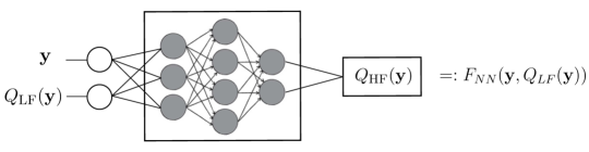
Figure 2: A schematic representation of NN1. It takes the input data $\{({\bf y}^{(i)},Q_{LF}^{(i)})\}_{i=1}^{M_{1}}$ and the output data $\{Q_{HF}^{(i)}\}_{i=1}^{M_{1}}$ to learn the correlation function $F({\bf y},Q_{LF}({\bf y}))$.

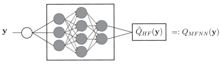
Figure 3: A schematic representation of NN2. It takes the input-output data $\{({\bf y}^{(i)},\hat{Q}_{HF}^{(i)})\}_{i=1}^{M}$ generated by NN1 to learn the high-fidelity quantity $Q_{HF}({\bf y})$.

We note that higher statistical moments may also be computed by taking the sample average of higher powers of the approximated quantity in the last step of the algorithm.

Remark 1.

If we simply take $M=0$, skip steps 1 to 6 above, and compute $N$ realizations of $Q$ directly by the high-fidelity model, we arrive at the classical MC sampling estimation

$${\mathbb{E}}[Q]\approx{\mathcal{A}}_{HFMC}:=\frac{1}{N}\sum_{i=1}^{N}Q_{HF}({\bf y}^{(i)}).$$ (7)

Remark 2.

The two networks (NN1 and NN2) are trained based on two training data sets of different size: NN1 uses $M_{1}$ data points, while NN2 uses $M>M_{1}$ data points. This may amount to two networks with different architectures. For instance, we may consider a simpler architecture (e.g. with a smaller number of layers/nurons) for NN1 compared to NN2, as the former uses less training data points than the latter. While this is true, we do not expect a large difference between the architectures of NN1 and NN2, as both networks learn the very same quantities $F$ and ${Q}_{HF}$ and hence need to have comparable complexities. This in turn imposes a restriction on the ratio $r=M_{1}/M<1$, that is, $r$ cannot be too small. We need $M_{1}$ to be large enough to ensure the accuracy of NN1. For instance, the numerical examples in Section 4 use $r=0.25$. It is to be noted that in cases when $r\ll 1$, for instance when we can afford only a few high-fidelity solves, the proposed construction may fail to deliver accurate predictions. We are currently working on a modified construction that enables accurate predictions even in the case $r\ll 1$, to be presented elsewhere.

Remark 3.

A recently proposed strategy [23] also employs NNs to construct multi-fidelity regression models. The construction in [23] has two major components. First, it uses a combination of a linear and nonlinear relation between the low- and high-fidelity models: $Q_{HF}({\bf y})=F_{L}({\bf y},Q_{LF}({\bf y}))+F_{NL}({\bf y},Q_{LF}({\bf y}))$. Next, it trains three NNs: one low-fidelity NN for approximating the low-fidelity model, and two high-fidelity NNs for learning the linear and nonlinear functions $F_{L}$ and $F_{NL}$. Consequently, each evaluation of $Q_{HF}({\bf y})$ would need all three networks to be evaluated. Our construction differs from [23] in both components. Instead of the combination of a linear and a nonlinear function, we employ a general (possibly nonlinear) function $F$ in (3). Such a general function can model both linear and nonlinear relations between the two models. Consequently, instead of training and evaluating two networks in [23], one for $F_{L}$ and one for $F_{NL}$, here we need only one network to learn $F$. This choice is motivated by the following observation: a neural network that captures the (complex) nonlinear features of a function can also capture its (simple) linear features without the need to add many extra layers/neurons. Moreover, our construction changes the training order proposed in [23] in the following way. While in [23] the first network uses only low-fidelity data and the second and third networks use both low-fidelity and high-fidelity data, here the first network uses both low-fidelity and high-fidelity data, and the second network uses only high-fidelity data. This change in the order of training data makes the ultimate evaluations “independent” of the first network. The first network NN1 is only used to generate additional training data for the second network NN2, and hence it will be evaluated only a few times. The two trained networks can therefore be separated, and only the second network NN2 needs to be evaluated for each evaluation of $Q_{HF}({\bf y})$. As a result, compared to [23], the new construction would save one network training and two network evaluations. Hence, the new construction may be superior in terms of both training costs and evaluation costs without sacrificing accuracy.

3.4 Approximation error

The approximation (6) involves two separate estimations: 1) the estimation of $Q$ by the surrogate model $Q_{MFNN}$ at a set of $N$ realizations of ${\bf y}$, and 2) the estimation of the integral by a sum of $N$ terms. Correspondingly, we may split the total error into two parts:

$$\varepsilon:=|{\mathbb{E}}[Q({\bf y})]-{\mathcal{A}}_{MFNNMC}|\leq\underbrace{|{\mathbb{E}}[Q({\bf y})]-{\mathbb{E}}[Q_{MFNN}({\bf y})]|}_{\varepsilon_{I}}+\underbrace{|{\mathbb{E}}[Q_{MFNN}({\bf y})]-{\mathcal{A}}_{MFNNMC}|}_{\varepsilon_{II}}.$$

The first error term $\varepsilon_{I}$ is deterministic and corresponds to the error in the approximation of $Q({\bf y})$ by the multi-fidelity neural network surrogate model $Q_{MFNN}({\bf y})$. Two sources contribute to this error: 1) the structure of NN2, including the number of layers and neurons, activation functions, and the regularization and optimization techniques and parameters used to train the network, and 2) the quantity and quality of the data used to train NN2, i.e. the number $M$ and location of the input points $\{{\bf y}^{(i)}\}_{i=1}^{M}\in Y_{I}\cup Y_{II}\subset\Gamma$ and the accuracy of the approximate realizations $\{\hat{Q}_{HF}^{(i)}\}_{i=1}^{M}$. The accuracy of the output data $\{\hat{Q}_{HF}^{(i)}\}_{i=1}^{M}$ given in (5) is determined by the error in approximating the QoI by the high-fidelity model, i.e. the error in $Q({\bf y})\approx Q_{HF}({\bf y})$ that satisfies (2), and the error in approximating the high-fidelity quantity by NN1, i.e. the error in $Q_{HF}({\bf y})\approx F_{NN}({\bf y},Q_{LF}({\bf y}))$. The latter in turn depends on two factors: i) the structure of NN1, and ii) the quantity and quality of the data used to train NN1, i.e. the number $M_{1}$ and location of the input points $\{{\bf y}^{(i)}\}_{i=1}^{M_{1}}\in Y_{I}\subset\Gamma$ and the accuracy of the approximate realizations $\{Q_{HF}^{(i)}\}_{i=1}^{M_{1}}$, which again satisfies (2). In summary, the first error term $\varepsilon_{I}$ depends on the structures of the two trained neural networks NN1 and NN2, the choice of the sets $Y_{I}$ and $Y_{II}$, and the error in the approximation of $Q$ by the high-fidelity model satisfying (2). As mentioned in Section 3.2, the precise dependence of the output error of a trained network on the network structure and the choice of input training data is still an open problem. However, thanks to the universal approximation theorem (see e.g. [16]), we may assume that there exist neural networks NN1 and NN2 that deliver predictions $Q_{MFNN}$ that are as accurate as the output training data $Q_{HF}$. More precisely, we assume that with a proper selection of network structure and input training data, we have

$$\varepsilon_{I}\leq C\,h_{HF}^{q}.$$ (8)

It is to be noted that while the universal approximation theorem states that there exists a network that can approximate a function within a desired tolerance, it does not tell how to construct such a network. Hence, we cannot a priori guarantee that the networks that we train would produce an error satisfying (8). In practice, we may need more validation data sets to reduce the possibility that (8) does not hold.

The second error term $\varepsilon_{II}$ is a quadrature error due to approximating the integral by a sum. In the particular case of MC sampling, since ${\mathcal{A}}_{MFNNMC}$ is a statistical term, $\varepsilon_{II}$ is referred to as the statistical error. By the central limit theorem (see e.g. [9]), we know that for large $N$ the distribution of the term ${\mathbb{E}}[Q_{MFNN}({\bf y})]-{\mathcal{A}}_{MFNNMC}$ will approach a normal distribution with mean zero and variance $\sqrt{{\mathbb{V}}[Q_{MFNN}]/N}$. Consequently, the error $\varepsilon_{II}$ satisfies

$$P\left(\varepsilon_{II}\leq c_{\alpha}\,\sqrt{\frac{{\mathbb{V}}[Q_{MFNN}]}{N}}\,\right)\rightarrow 2\phi(c_{\alpha})-1,\qquad\text{as}\ \ N\rightarrow\infty,$$ (9)

where $P$ is a probability measure, and $\phi(c_{\alpha})=\frac{1}{\sqrt{2\pi}}\int_{-\infty}^{c_{\alpha}}\exp(-\tau^{2}/2)d\tau$ is the cumulative density function of a standard normal random variable evaluated at a given confidence level $c_{\alpha}>0$. Clearly, the larger the confidence level, the higher the probability that the inequality $\varepsilon_{II}\leq c_{\alpha}\,\sqrt{{\mathbb{V}}[Q_{MFNN}]/N}$ holds.

We often need the approximation ${\mathcal{A}}_{MFNNMC}$ to be accurate within a desired small tolerance $\varepsilon_{\footnotesize{\text{TOL}}}>0$ and with a pre-assigned small failure probability $\alpha\in(0,1)$, that is,

$$P(\varepsilon\leq\varepsilon_{\footnotesize{\text{TOL}}})=1-\alpha.$$

To achieve this, we may first split the tolerance between the deterministic and statistical errors by introducing a splitting parameter $\theta\in(0,1)$ and require that

$$\varepsilon_{I}\leq(1-\theta)\varepsilon_{\footnotesize{\text{TOL}}},\qquad P(\varepsilon_{II}\leq\theta\,\varepsilon_{\footnotesize{\text{TOL}}})=1-\alpha.$$ (10)

From (8) and the first inequality in (10) we obtain $h_{HF}$ by requiring $Ch_{HF}^{q}\leq(1-\theta)\,\varepsilon_{\footnotesize{\text{TOL}}}$. Moreover, comparing (9) and the second inequality in (10), we set $2\phi(c_{\alpha})-1=1-\alpha$ and obtain the confidence level $c_{\alpha}=\phi^{-1}(1-\alpha/2)$. Then, the number of samples $N$ will be obtained by requiring $c_{\alpha}\,\sqrt{{\mathbb{V}}[Q_{MFNN}]/N}\leq\theta\,\varepsilon_{\footnotesize{\text{TOL}}}$. Finally, we get

$$h_{HF}\propto\varepsilon_{\footnotesize{\text{TOL}}}^{1/q},\qquad N\propto\varepsilon_{\footnotesize{\text{TOL}}}^{-2}.$$

It is to be noted that (10) guarantees that $P(\varepsilon>\varepsilon_{\footnotesize{\text{TOL}}})\leq\alpha$, which is more conservative than what we need: $P(\varepsilon>\varepsilon_{\footnotesize{\text{TOL}}})=\alpha$. In order to avoid too conservative considerations, we should select $h_{HF}$ so that the deterministic error $\varepsilon_{I}$ is as close as possible to $(1-\theta)\varepsilon_{TOL}$.

3.5 Computational cost

Let $W_{LF}$ and $W_{HF}$ denote the computational cost of evaluating $Q_{LF}$ and $Q_{HF}$ in (1) at a single realization of ${\bf y}$, respectively. Let further $W_{Ti}$ and $W_{Pi}$, with $i=1,2$, be the training cost and the cost of evaluating NN$i$ at a single realization of ${\bf y}$, respectively. The total cost of computing the estimator ${\mathcal{A}}_{MFNNMC}$ in (6) will then be

$$W_{MFNNMC}=M\,W_{LF}+M_{1}\,W_{HF}+W_{T1}+M_{2}\,W_{P1}+W_{T2}+N\,W_{P2}.$$ (11)

We will now discuss the efficiency of the proposed sampling method and compare its cost with the cost of the classical high-fidelity MC estimator ${\mathcal{A}}_{HFMC}$ formulated in (7), which is

$$W_{HFMC}=N\,W_{HF}.$$ (12)

In many problems, we often need to obtain accurate predictions within small tolerances $\varepsilon_{\footnotesize{\text{TOL}}}\ll 1$. To achieve this within the framework of MC sampling, we usually need a very large number of samples $N\propto\varepsilon_{\footnotesize{\text{TOL}}}^{-2}\gg 1$. This is because the statistical error in MC sampling is proportional to $N^{-1/2}$ and hence decays very slowly as $N$ increases, as discussed above. The classical high-fidelity MC sampling would therefore be very expensive as it requires a very large number $N$ of expensive high-fidelity problems to be solved. For instance, suppose $W_{HF}\propto h_{HF}^{-\gamma}$, where $\gamma>0$ is related to the time-space dimension of the ODE/PDE problem and the discretization technique used to solve the problem. Then, noting $h_{HF}\propto\varepsilon_{\footnotesize{\text{TOL}}}^{1/q}$, the cost of MC sampling (12) reads

$$W_{HFMC}\propto\varepsilon_{\footnotesize{\text{TOL}}}^{-(2+\gamma/q)}.$$ (13)

In the new sampling algorithm proposed here, however, we may achieve dramatic savings in computational cost by replacing many (i.e. $N$) expensive high-fidelity ODE/PDE solves needed in MC sampling with the same number of fast neural network computations and only a few (i.e. $M_{1}$) high-fidelity solves. For this to work, we would need: 1) the number $M$ of required training data to be much less than the number $N$ of required MC samples; 2) the cost $W_{P2}$ of evaluating NN2 to be much less than the cost $W_{HF}$ of a complex ODE/PDE solve; and 3) the total training cost $W_{T1}+W_{T2}$ to be negligible compared to the cost of solving $N$ complex ODE/PDE problems. A few observations addressing each of the above three requirements follow. See also Section 4 for numerical verifications.

• While there is currently no results on the dependency of the number of required training data on accuracy, we have observed through numerical experiments that $M$ depends mildly on the tolerance, i.e. $M\propto\varepsilon_{\footnotesize{\text{TOL}}}^{-p}$, where $p\in[0,1)$ is small. A similar observation has also been made in [1]. A comparison between $M\propto\varepsilon_{\footnotesize{\text{TOL}}}^{-p}$ and $N\propto\varepsilon_{\footnotesize{\text{TOL}}}^{-2}$ suggests that the smaller the tolerance, the larger the ratio $N/M$. Consequently, the term $M\,W_{LF}+M_{1}\,W_{HF}$ in (11) will be proportional to $\varepsilon_{\footnotesize{\text{TOL}}}^{-(p+\gamma/q)}$, which is much less than $N\,W_{HF}$ and hence negligible at small tolerance levels.

• The cost of evaluating a neural network depends on the network architecture, i.e. the number of hidden layers and neurons and the type of activation functions. The evaluation of a network mainly involves simple matrix-vector operations and the application of activation functions. Crucially, the evaluation cost is independent of the complexity of the ODE/PDE problem. In particular, for QoIs that can be well approximated by a network with a few hidden layers and hundreds of neurons, we would get $W_{Pi}\ll W_{HF}$, with $i=1,2$. Indeed, in such cases, the more complex the high-fidelity problem and the more expensive computing the high-fidelity quantity, the larger the ratio $W_{HF}/W_{Pi}$.

• The cost of training the two networks depends on the number of training data, network structure, and the cost of solving their corresponding optimization problems. Importantly, it is a one-time cost. In particular, we have observed through numerical experiments that as the tolerance decreases and $N$ increases, this cost becomes negligible.

In summary, for the ODE/PDE problems and QoIs where the above three requirements hold, we may obtain for small tolerances:

$$W_{MFNNMC}\propto\varepsilon_{\footnotesize{\text{TOL}}}^{-\max(2,\,p+\gamma/q)}.$$ (14)

Comparing (13) and (14), we consider two cases: 1) if $p+\gamma/q\leq 2$, then $W_{MFNNMC}\propto\varepsilon_{\footnotesize{\text{TOL}}}^{-2}$ will be much smaller than $W_{HFMC}$, and 2) if $p+\gamma/q>2$, then $W_{MFNNMC}\propto\varepsilon_{\footnotesize{\text{TOL}}}^{-(p+\gamma/q)}$ will be much smaller than $W_{HFMC}$ as long as $p<2$. Importantly, the smaller the tolerance $\varepsilon_{\text{TOL}}$, the more gain in computational cost over MC sampling.

4 Numerical Examples

In this section we present two numerical examples: an ODE problem and a PDE problem. All codes are written in Python and run on a single CPU in order to have a fair comparison between the proposed method and MC sampling. We use Keras [6], which is an open-source neural-network library written in Python, to construct the neural networks. It is to be noted that all CPU times are measured by time.clock() in Python.

4.1 An ODE problem

Consider the following parametric initial value problem (IVP)

$$\begin{array}[]{ll}u_{t}(t,y)+0.5u(t,y)=f(t,y),&\qquad t\in[0,T],\quad y\in\Gamma\subset{\mathbb{R}},\\ u(0,y)=g(y).&\end{array}$$ (15)

where $y\in\Gamma$ is a uniformly distributed random variable on $\Gamma=[-1,1]$, and the force term $f$ and the initial data $g$ are so that the exact solution to the IVP (15) is

$$u(t,y)=0.5+2\sin(12y)+6\sin(2t)\sin(10y)(1+2y^{2}).$$

Our goal is to approximate the expectation ${\mathbb{E}}[Q(y)]$, where $Q(y)=|q(y)|=|u(T,y)|$ with $T=100$, by the multi-fidelity estimator ${\mathcal{A}}_{MFNNMC}$ in (6) and compare its performance with the high-fidelity MC estimator ${\mathcal{A}}_{HFMC}$ in (7). We use the closed form of solution to measure errors and will compare the cost of the two methods subject to the same accuracy constraint.

Suppose that we have the second-order accurate Runge-Kutta (RK2) time-stepper as the deterministic solver to compute realizations of $q_{LF}(y)$ and $q_{HF}(y)$ using time steps $h_{LF}$ and $h_{HF}$, respectively. Consider the relative error in the approximation

$$\varepsilon_{\text{rel}}:=|{\mathbb{E}}[Q(y)]-{\mathcal{A}}|/|{\mathbb{E}}[Q(y)]|,$$

where the estimator ${\mathcal{A}}$ is either ${\mathcal{A}}_{MFNNMC}$ or ${\mathcal{A}}_{HFMC}$. Given a $1\%$ failure probability ($\alpha=0.01$) and a decreasing sequence of tolerances $\varepsilon_{\footnotesize{\text{TOL}}}=10^{-2},10^{-3},10^{-4}$, a simple error analysis similar to the analysis in Section 3.4 and verified by numerical computations gives the minimum number of realizations $N$ and the maximum time step $h_{HF}$ for the high-fidelity model required to achieve $P(\varepsilon_{\text{rel}}\leq\varepsilon_{\footnotesize{\text{TOL}}})=0.99$. We choose a fixed time step $h_{LF}=0.5$ for the low-fidelity model at all tolerance levels. Table 1 summarizes the numerical parameters $(N,h_{HF},h_{LF})$ and the CPU time of evaluating single realizations of $q_{LF}$ and $q_{HF}$.

Table 1: Required number of realizations and time steps to achieve $P(\varepsilon_{\text{rel}}\leq\varepsilon_{\footnotesize{\text{TOL}}})=0.99$.

$\varepsilon_{\footnotesize{\text{TOL}}}$	$N$	$h_{HF}$	$W_{HF}$	$h_{LF}$	$W_{LF}$
$10^{-2}$	$1.35\times 10^{5}$	0.1	$2.24\times 10^{-4}$	0.5	$4.36\times 10^{-5}$
$10^{-3}$	$1.35\times 10^{7}$	0.025	$7.21\times 10^{-4}$	0.5	$4.36\times 10^{-5}$
$10^{-4}$	$1.35\times 10^{9}$	0.01	$2.20\times 10^{-3}$	0.5	$4.36\times 10^{-5}$

Following the algorithm in Section 3.3, we first generate a set of $M=M_{1}+M_{2}$ points $y^{(i)}\in[-1,1]$, with $i=1,\dotsc,M$, collected into two disjoint sets $Y_{I}$ and $Y_{II}$. Figure 4 shows a schematic representation of the selection of points. We choose the points to be uniformly placed on the interval $[-1,1]$. We then select every 4th point to be in the set $Y_{I}$ (magenta circles) and collect the rest of the points in the set $Y_{II}$ (blue triangles). This implies $M_{2}\approx 3\,M_{1}$, meaning that we will need to compute the quantity $q(y)$ by the high-fidelity model, that is RK2 using time step $h_{HF}$, at only a quarter of points $M/4$. The number of points $M$ will be chosen based on the desired tolerance, slightly increasing as the tolerance decreases.

Figure 4: A schematic representation of the selected points. Magenta circles represent the points in $Y_{I}$, where only the high-fidelity quantity is computed. The blue triangles represent the points in $Y_{II}$. The low fidelity quantity is computed at all points in $Y_{I}\cup Y_{II}$.

We will use the same architecture for the two networks NN1 and NN2 and keep them fixed at all tolerances. Precisely, we choose feed-forward networks with 4 hidden layers, where each layer contains 20 neurons. We use ReLU activation function for the hidden layers and the identity activation function for the output layer of both networks. It is to be noted that NN1 has two input neurons, while NN2 has one input neuron. Both networks have one output neuron. For the training process, we employ the quadratic cost function (or the mean squared error) and use the Adam optimization technique with a fixed learning rate $\eta=0.002$. We note that instead of a fixed learning rate, one may alternatively split the available $M$ data points into training and validation sets and tune the learning rate parameter. For this ODE example, we do not use any validation set as the choice $\eta=0.002$ produces satisfactory results both in terms of efficiency and accuracy. We also do not use any regularization technique. Table 2 summarizes the number of training data $M=M_{1}+M_{2}$, the number of epochs $N_{\text{epoch}}$, batch size $N_{\text{batch}}$, and the CPU time of training and evaluating the two networks for different tolerances. We observe that the number of training data satisfies $M\propto\varepsilon_{\footnotesize{\text{TOL}}}^{-p}$ with $p=0.5$. It is also to be noted that while using a different architecture for each network and other choices of network parameters (e.g. number of layers/ neurons and learning rates) may give more efficient networks, the selected architectures and parameters here, following the general guidelines in [3, 12], produce satisfactory results in terms of efficiency (see Figure 7) and accuracy (see Figure 8).

Table 2: The number of training data and training and evaluation time of the two networks.

			NN1				NN2
$\varepsilon_{\footnotesize{\text{TOL}}}$	$M_{1}$	$M_{2}$	$N_{\text{epoch}}$	$N_{\text{batch}}$	$W_{T_{1}}$	$W_{P_{1}}$	$N_{\text{epoch}}$	$N_{\text{batch}}$	$W_{T_{2}}$	$W_{P_{1}}$
$10^{-2}$	61	180	100	10	10.98	$3.57\times 10^{-5}$	1800	40	147.44	$3.55\times 10^{-5}$
$10^{-3}$	201	600	1000	30	81.13	$7.77\times 10^{-5}$	5000	80	1623.41	$4.38\times 10^{-5}$
$10^{-4}$	801	2400	5000	100	768.30	$8.39\times 10^{-5}$	30000	100	10096.63	$3.73\times 10^{-5}$

Figure 5 shows the low-fidelity and high-fidelity quantities versus $y\in[-1,1]$ (solid lines) and the data (circle and triangle markers) available in the case $\varepsilon_{\footnotesize{\text{TOL}}}=10^{-2}$. Figure 6 (left) shows the generated high-fidelity data by the trained network NN1, and Figure 6 (right) shows the predicted high-fidelity quantity by the trained network NN2 for tolerance $\varepsilon_{\footnotesize{\text{TOL}}}=10^{-2}$.

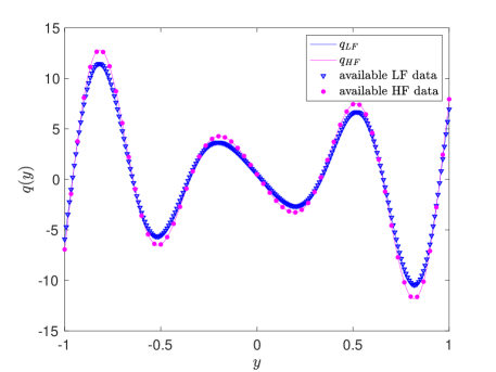
Figure 5: The low-fidelity and high-fidelity quantities versus $y\in[-1,1]$ (solid lines) and the available data (markers) in the case $\varepsilon_{\footnotesize{\text{TOL}}}=10^{-2}$. There are $M_{1}=61$ high-fidelity and $M=241$ low-fidelity data points, represented by circles and triangles, respectively.

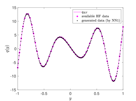
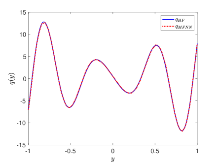
Figure 6: Outputs of the trained networks for $\varepsilon_{\footnotesize{\text{TOL}}}=10^{-2}$. Left: generated data by the trained network NN1. Right: predicted quantity by the trained network NN2.

Figure 7 shows the CPU time as a function of tolerance. The computational cost of classical MC sampling is ${\mathcal{O}}(\varepsilon_{\footnotesize{\text{TOL}}}^{-2.5})$, following (13) and noting that the order of accuracy of RK2 is $q=2$ and the time-space dimension of the problem is $\gamma=1$. On the other hand, if we only consider the prediction time of the proposed multi-fidelity method, excluding the training costs, the cost of the proposed method is proportional to $\varepsilon_{\footnotesize{\text{TOL}}}^{-2}$ which is much less than the cost of MC sampling. When adding the training costs, we observe that although for large tolerances the training cost is large, as the tolerance decreases the training costs become negligible compared to the total CPU time. Overall, the cost of the proposed method approaches ${\mathcal{O}}(\varepsilon_{\footnotesize{\text{TOL}}}^{-2})$ as tolerance decreases, and hence, the smaller the tolerance, the more gain in computational cost when employing the proposed method over MC sampling. This can also be seen by (14) where $\max(2,p+\gamma/q)=\max(2,0.5+0.5)=2$.

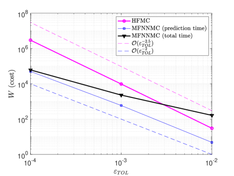
Figure 7: CPU time versus tolerance. For large tolerances the training cost is dominant, making the cost of MFNNMC more than the cost of HFMC. However, as tolerance decreases, the training cost becomes negligible and the cost of MFNNMC approaches ${\mathcal{O}}(\varepsilon_{\footnotesize{\text{TOL}}}^{-2})$.

Finally, Figure 8 shows the relative error as a function of tolerance for the proposed method, verifying that the tolerance is met with 1$\%$ failure probability.

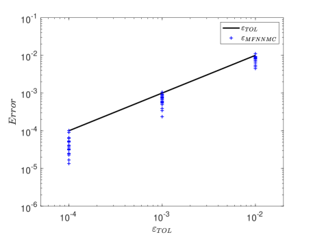
Figure 8: Relative error as a function of tolerance, verifying that the tolerance is met with 1$\%$ failure probability. The “+” markers correspond to 20 simulations at each tolerance level.

4.2 A PDE problem

Consider the following parametric initial-boundary value problem (IBVP)

$$\begin{array}[]{ll}u_{tt}(t,{\bf x},{\bf y})-\Delta_{\bf x}u(t,{\bf x},{\bf y})=f(t,{\bf x},{\bf y}),&\ \ \ (t,{\bf x},{\bf y})\in[0,T]\times D\times\Gamma,\\ u(0,{\bf x},{\bf y})=g_{1}({\bf x},{\bf y}),\ \ u_{t}(0,{\bf x},{\bf y})=g_{2}({\bf x},{\bf y}),&\ \ \ (t,{\bf x},{\bf y})\in\{0\}\times D\times\Gamma,\\ u(t,{\bf x},{\bf y})=g_{b}(t,{\bf x},{\bf y}),&\ \ \ (t,{\bf x},{\bf y})\in[0,T]\times\partial D\times\Gamma,\end{array}$$ (16)

where $t\in[0,T]$ is the time, ${\bf x}=(x_{1},x_{2})\in D$ is the vector of spatial variables on a square domain $D=[-1,1]^{2}$, and ${\bf y}=(y_{1},y_{2})\in\Gamma$ is a vector of two uniformly distributed random variables on $\Gamma=[10,11]\times[4,6]$. We select the force term $f$ and the initial-boundary data $g_{1},g_{2},g_{b}$ so that the exact solution to the IBVP (16) is

$$u(t,{\bf x},{\bf y})=\sin(y_{1}\,t-y_{2}\,x_{1})\,\sin(y_{2}\,x_{2}).$$

Our goal is to approximate the expectation ${\mathbb{E}}[Q(y)]$, where $Q({\bf y})=|q({\bf y})|=|u(T,{\bf x}_{Q},{\bf y})|$ with $T=30$ and ${\bf x}_{Q}=(0.5,0.5)$, by the multi-fidelity estimator ${\mathcal{A}}_{MFNNMC}$ in (6) and compare its performance with the high-fidelity MC estimator ${\mathcal{A}}_{HFMC}$ in (7). We use the closed form of solution to measure errors and will compare the cost of the two methods subject to the same accuracy constraint.

Suppose that we have a second-order accurate (in both time and space) finite difference scheme as the deterministic solver to compute realizations of $q_{LF}({\bf y})$ and $q_{HF}({\bf y})$ using a uniform grid with grid lengths $h_{LF}$ and $h_{HF}$, respectively. We use the time step $\Delta t=h/2$ to ensure stability of the numerical scheme, where the grid length $h$ is either $h_{LF}$ or $h_{HF}$, depending on the level of fidelity. Consider the absolute error in the approximation

$$\varepsilon_{\text{abs}}:=|{\mathbb{E}}[Q({\bf y})]-{\mathcal{A}}|,$$

where the estimator ${\mathcal{A}}$ is either ${\mathcal{A}}_{MFNNMC}$ or ${\mathcal{A}}_{HFMC}$. Given a $1\%$ failure probability ($\alpha=0.01$) and a decreasing sequence of tolerances $\varepsilon_{\footnotesize{\text{TOL}}}=10^{-1},10^{-2},10^{-3}$, a simple error analysis similar to the analysis in Section 3.4 and verified by numerical computations gives the minimum number of realizations $N$ and the maximum grid length $h_{HF}$ for the high-fidelity model required to achieve $P(\varepsilon_{\text{abs}}\leq\varepsilon_{\footnotesize{\text{TOL}}})=0.99$. Table 3 summarizes the numerical parameters $(N,h_{HF},h_{LF})$ and the CPU time of evaluating single realizations of $q_{LF}$ and $q_{HF}$.

Table 3: Required number of realizations and grid lengths to achieve $P(\varepsilon_{\text{abs}}\leq\varepsilon_{\footnotesize{\text{TOL}}})=0.99$.

$\varepsilon_{\footnotesize{\text{TOL}}}$	$N$	$h_{HF}$	$W_{HF}$	$h_{LF}$	$W_{LF}$
$10^{-1}$	$1.5\times 10^{2}$	$1/32$	$0.67$	$1/20$	$0.21$
$10^{-2}$	$1.5\times 10^{4}$	$1/128$	$29.75$	$1/32$	$0.67$
$10^{-3}$	$1.5\times 10^{6}$	$1/320$	$708.21$	$1/32$	$0.67$

Following the algorithm in Section 3.3, we first generate a uniform grid of $M=M_{1}+M_{2}$ points ${\bf y}^{(i)}\in[10,11]\times[4,6]$, with $i=1,\dotsc,M$, collected into two disjoint sets $Y_{I}$ and $Y_{II}$. We select the two disjoint sets so that $M_{2}\approx 3\,M_{1}$, meaning that we will need to compute the quantity $q({\bf y})$ by the high-fidelity model with grid length $h_{HF}$ at only a quarter of points $M/4$. The number of points $M$ will be chosen based on the desired tolerance, slightly increasing as the tolerance decreases.

We will use the same architecture for the two networks NN1 and NN2 and keep them fixed at all tolerance levels. Precisely, we choose feed-forward networks with 4 hidden layers, where each layer contains 30 neurons. We use ReLU activation function for the hidden layers and the identity activation function for the output layer of both networks. It is to be noted that NN1 has three input neurons, while NN2 has two input neurons. Both networks have one output neuron. For the training process, we split the available $M$ data points into a training set (90$\%$ of $M$) and a validation set (10$\%$ of $M$). We apply pre-processing transformations to the input data points before they are presented to the two networks. Precisely, we transform the points from $[10,11]\times[4,6]$ to the unit square $[0,1]^{2}$. We then employ the quadratic cost function and use the Adam optimization technique with an initial learning rate $\eta=0.005$ that will be adaptively tuned using the validation set. We do not use any regularization technique. Table 4 summarizes the number of training and validation data $M=M_{1}+M_{2}$, the number of epochs $N_{\text{epoch}}$, batch size $N_{\text{batch}}$, and the CPU time of training and evaluating the two networks for different tolerances. We note that the number of training data satisfies $M\propto\varepsilon_{\footnotesize{\text{TOL}}}^{-p}$ with $p=0.2$.

Table 4: The number of training data and training and evaluation time of the two networks.

			NN1				NN2
$\varepsilon_{\footnotesize{\text{TOL}}}$	$M_{1}$	$M_{2}$	$N_{\text{epoch}}$	$N_{\text{batch}}$	$W_{T_{1}}$	$W_{P_{1}}$	$N_{\text{epoch}}$	$N_{\text{batch}}$	$W_{T_{2}}$	$W_{P_{1}}$
$10^{-1}$	848	2407	500	50	326.57	$4.10\times 10^{-4}$	500	50	1069.26	$4.00\times 10^{-4}$
$10^{-2}$	1281	3680	500	50	487.28	$4.75\times 10^{-4}$	1000	50	2904.67	$4.60\times 10^{-4}$
$10^{-3}$	1976	5725	1000	50	1415.44	$4.80\times 10^{-4}$	2000	50	9743.86	$4.70\times 10^{-4}$

Figure 9 shows the true high-fidelity quantity (left) and the predicted high-fidelity quantity by the trained network NN2 (right) for tolerance $\varepsilon_{\footnotesize{\text{TOL}}}=10^{-2}$.

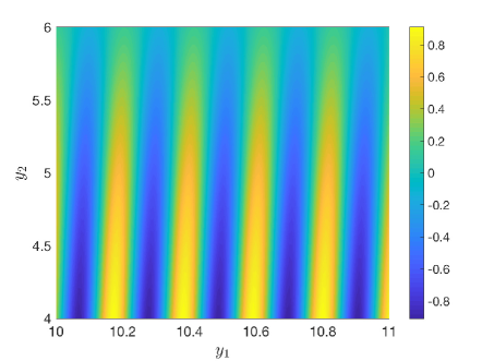
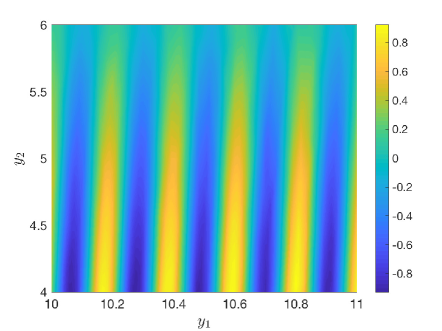
Figure 9: High-fidelity quantity $q_{HF}({\bf y})$ for $\varepsilon_{\footnotesize{\text{TOL}}}=10^{-2}$. Left: true quantity. Right: predicted quantity by the trained network NN2.

Figure 10 shows the CPU time as a function of tolerance. The computational cost of classical MC sampling is proportional to $\varepsilon_{\footnotesize{\text{TOL}}}^{-3.5}$, following (13) and noting that the order of accuracy of the finite difference scheme is $q=2$ and the time-space dimension of the problem is $\gamma=3$. On the other hand, if we only consider the prediction time of the proposed multi-fidelity method, excluding the training costs, the cost of the proposed method is proportional to $\varepsilon_{\footnotesize{\text{TOL}}}^{-2}$ which is much less than the cost of MC sampling. When adding the training costs, we observe that although for large tolerances the training cost is large, as the tolerance decreases the training costs become negligible compared to the total CPU time. Overall, the cost of the proposed method approaches ${\mathcal{O}}(\varepsilon_{\footnotesize{\text{TOL}}}^{-2})$ as tolerance decreases, indicating orders of magnitude acceleration in computing the expectation compared to MC sampling. This convergence rate can also be seen by (14) where $\max(2,p+\gamma/q)=\max(2,0.2+1.5)=2$.

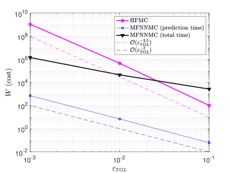
Figure 10: CPU time versus tolerance. For large tolerances the training cost is dominant, making the cost of MFNNMC more than the cost of HFMC. However, as tolerance decreases, the training cost becomes negligible and the cost of MFNNMC approaches ${\mathcal{O}}(\varepsilon_{\footnotesize{\text{TOL}}}^{-2})$.

Finally, Figure 11 shows the relative error as a function of tolerance for the proposed method, verifying that the tolerance is met with 1$\%$ failure probability.

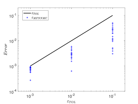
Figure 11: Relative error as a function of tolerance, verifying that the tolerance is met with 1$\%$ failure probability. The “+” markers correspond to 20 simulations at each tolerance level.

5 Conclusion

This work presents a multi-fidelity neural network surrogate sampling method for the uncertainty quantification of physical/biological systems described by systems of ODEs/PDEs. The proposed algorithm combines the approximation power of neural networks with the advantages of MC sampling in a multi-fidelity framework. For the numerical examples considered here, we observe dramatic savings in computational cost when the output predictions are desired to be accurate within small tolerances. More sophisticated numerical examples and a more comprehensive comparison between the proposed method and other advanced MC sampling techniques are subjects of current work and will be presented elsewhere. Other future directions include the extension of the proposed construction to training more than two networks using data sets at multiple levels of fidelity within multi-level and multi-index frameworks.

References

- [1] M. A. Akter. A Deep Learning Approach to Uncertainty Quantification. Master’s thesis, University of New Mexico, Albuquerque, New Mexico, 2019.
- [2] R. C. Aydin, F. A. Braeu, and C. J. Cyron. General multi-fidelity framework for training artificial neural networks with computational models. Frontiers in Materials, 6:1–14, 2019.
- [3] Y. Bengio. Practical recommendations for gradient-based training of deep architectures. In Müller KR. Montavon G., Orr G.B., editor, Neural Networks: Tricks of the Trades, pages 437–478. Springer, Berlin, 2012.
- [4] H. Bolcskei, P. Grohs, G. Kutyniok, and P. Petersen. Optimal approximation with sparsely connected deep neural networks. SIAM J. Mathematics of Data Science, 1:8–45, 2019.
- [5] L. Bottou, F. E. Curtis, and J. Nocedal. Optimization methods for large-scale machine learning. SIAM Rev., 60:223–311, 2018.
- [6] François Chollet et al. Keras. \urlhttps://keras.io, 2015.
- [7] K. A. Cliffe, M. B. Giles, R. Scheichl, and A. L. Teckentrup. Multilevel Monte Carlo methods and applications to elliptic PDEs with random coefficients. Comput. Visual Sci., 14:3–15, 2011.
- [8] M. G. Fernandez-Godino, C. Park, N. H. Kim, and R. T. Haftka. Review of multi-fidelity models. arXiv:1609.07196, 2016.
- [9] G. S. Fishman. Monte Carlo: Concepts, Algorithms, and Applications. Springer- Verlag, New York, 1996.
- [10] R. G. Ghanem and P. D. Spanos. Stochastic finite elements: A spectral approach. Springer, New York, 1991.
- [11] M. B. Giles. Multilevel Monte Carlo path simulation. Oper. Res., 56:607–617, 2008.
- [12] I. J. Goodfellow, Y. Bengio, and A. Courville. Deep Learning. MIT Press, Cambridge, MA, USA, 2016.
- [13] A. A. Gorodetsky, G. Geraci, M. Eldred, and J. D. Jakeman. A generalized approximate control variate framework for mulifidelity uncertainty quantification. arxiv.org/abs/1811.04988, 2019.
- [14] I. Gühring, G. Kutyniok, and P. Petersen. Error bounds for approximations with deep ReLU neural networks in norms. arxiv.org/abs/1902.07896, 2019.
- [15] A.-L. Haji-Ali, F. Nobile, and R. Tempone. Multi-index Monte Carlo: when sparsity meets sampling. Numerische Mathematik, 132:767–806, 2016.
- [16] K. Hornik, M. Stinchcombe, and H. White. Multilayer feedforward networks are universal approximators. Journal Neural Networks, 2:359–366, 1989.
- [17] T. Y. Hou and X. Wu. Quasi-Monte Carlo methods for elliptic PDEs with random coefficients and applications. J. Comput. Phys., 230:3668–3694, 2011.
- [18] Gianluca Geraci Alex Gorodetsky John D. Jakeman, Michael Eldred. Adaptive multi-index collocation for uncertainty quantification and sensitivity analysis. arXiv:1909.13845, 2019.
- [19] J. Kiefer and J. Wolfowitz. Stochastic estimation of the maximum of a regression function. Ann. Math. Statist., 23:462–466, 1952.
- [20] D. P. Kingma and J. Ba. Adam: A method for stochastic optimization. arXiv:1412.6980v9, 2017.
- [21] F. Y. Kuo, C. Schwab, and I. H. Sloan. Multi-level quasi-Monte Carlo finite element methods for a class of elliptic PDEs with random coefficients. Foundations of Computational Mathematics, 15:411–449, 2015.
- [22] D. Liu and Y. Wang. Multi-fidelity physics-constrained neural network and its application in materials modeling. Journal of Mechanical Design, 141:121403, 2019.
- [23] X. Meng and G. E. Karniadakis. A composite neural network that learns from multi-fidelity data: Application to function approximation and inverse PDE problems. Journal of Computational Physics, 401: 20160751, 2020.
- [24] H. N. Mhaskar and T. Poggio. Deep vs. shallow networks: An approximation theory perspective. Analysis and Applications, 14:829–848, 2016.
- [25] H. Montanelli and Q. Du. New error bounds for deep ReLU networks using sparse grids. SIAM J. Mathematics of Data Science, 1:78–92, 2019.
- [26] M. Motamed and D. Appelö. A multi-order discontinuous Galerkin Monte Carlo method for hyperbolic problems with stochastic parameters. SIAM J. Numer. Anal., 56:448–468, 2018.
- [27] M. Motamed, F. Nobile, and R. Tempone. A stochastic collocation method for the second order wave equation with a discontinuous random speed. Numer. Math., 123:493–536, 2013.
- [28] M. Motamed, F. Nobile, and R. Tempone. Analysis and computation of the elastic wave equation with random coefficients. Computers and Mathematics with Applications, 70:2454–2473, 2015.
- [29] F. Nobile, R. Tempone, and C. G. Webster. A sparse grid stochastic collocation method for partial differential equations with random input data. SIAM J. Numer. Anal., 46:2309–2345, 2008.
- [30] F. Nobile and F. Tesei. A multi level Monte Carlo method with control variate for elliptic PDEs with log-normal coefficients. Stoch PDE: Anal Comp, 3:398–444, 2015.
- [31] P. Perdikaris, M. Raissi, A. Damianou, N. Lawrence, and G. E. Karniadakis. Nonlinear information fusion algorithms for data-efficient multi-fidelity modelling. Proc. R. Soc. A, 473: 20160751, 2017.
- [32] P. Petersen and F. Voigtlaender. Optimal approximation of piecewise smooth functions using deep ReLU neural networks. Neural Networks, 108:296–330, 2018.
- [33] H. Robbins and S. Monro. A stochastic approximation method. Ann. Math. Statist., 22:400–407, 1951.
- [34] D. E. Rumelhart, G. E. Hinton, and R. J. Williams. Learning representations by back-propagating errors. Nature, 323:533–536, 1986.
- [35] J. Schmidhuber. Deep learning in neural networks: An overview. Neural netw., 61:85–117, 2015.
- [36] C. Schwab and J. Zech. Deep learning in high dimension: Neural network expression rates for generalized polynomial chaos expansions in UQ. Analysis and Applications, 17:19–55, 2019.
- [37] A. Speight. A multilevel approach to control variates. Journal of Computational Finance, 12:3–27, 2009.
- [38] N. Srivastava, G. Hinton, A. Krizhevsky, I. Sutskever, and R. Salakhutdinov. Dropout: A simple way to prevent neural networks from overfitting. Journal of Machine Learning Research, 15:1929–1958, 2014.
- [39] T. J. Sullivan. Introduction to Uncertainty Quantification. Springer, 2015.
- [40] D. Xiu and J. S. Hesthaven. High-order collocation methods for differential equations with random inputs. SIAM J. Sci. Comput., 27:1118–1139, 2005.
- [41] D. Yarotsky. Error bounds for approximations with deep ReLU networks. Neural Networks, 94:103–114, 2017.