Effective low-dimensional dynamics of a mean-field coupled network of slow-fast spiking lasers.

Abstract

Low dimensional dynamics of large networks is the focus of many theoretical works, but controlled laboratory experiments are comparatively very few. Here, we discuss experimental observations on a mean-field coupled network of hundreds of semiconductor lasers, which collectively display effectively low-dimensional mixed mode oscillations and chaotic spiking typical of slow-fast systems. We demonstrate that such a reduced dimensionality originates from the slow-fast nature of the system and of the existence of a critical manifold of the network where most of the dynamics takes place. Experimental measurement of the bifurcation parameter for different network sizes corroborate the theory.

The collective dynamics of large ensembles of coupled systems is a far reaching research topic and striking natural examples of reduced dynamics dimensionality in large networks abound, like fireflies or applause synchronization Néda et al. (2000). One paradigmatic example is the synchronization of globally coupled phase oscillators as observed in the Kuramoto model Kuramoto (2012), whose relative simplicity has allowed tremendous progress (see e.g. Strogatz (2000)). Beyond this idealistic case, a particularly relevant situation is that of spiking nodes such as neurons, whose synchronization may play a key role in epilepsy Jiruska et al. (2013). Thus, many studies focus on the reduced dimensionality of the dynamics of networks of neuron models, see e.g. Mirollo and Strogatz (1990); Watanabe and Strogatz (1994); Zillmer et al. (2006); Olmi et al. (2014); Kotani et al. (2014); Montbrió et al. (2015); Pazó and Montbrió (2016), often enabled by the so-called Ott-Antonsen ansatz Ott and Antonsen (2008, 2009). In contrast to this rich theoretical literature, experimental observations are scarce. Here, we study the dynamics of a mean-field coupled network of chaotically spiking, dynamically coupled semiconductor lasers. We observe experimentally mixed mode oscillations and chaotic spiking in the mean field, which result from partial synchronization along the slow manifold of the network even in absence of synchronization of the fast dynamics of the nodes.

The analysis of optical model systems is often useful in nonlinear science, in particular about the synchronization of oscillators as shown in lasers in Nixon et al. (2011, 2012). With respect to neurosciences, optical analogues of neurons abound (recent references include Selmi et al. (2014); Hurtado and Javaloyes (2015); Sorrentino et al. (2015); Mesaritakis et al. (2016); Prucnal et al. (2016); Dolcemascolo et al. (2018)) but only very few nodes have been experimentally coupled: self-coupling with delay in Garbin et al. (2015); Romeira et al. (2016); Terrien et al. (2018), and two nodes in Yacomotti et al. (2002); Kelleher et al. (2010); Van Vaerenbergh et al. (2012); Deng et al. (2017). In contrast, we study a large network of 451 elements. The coupling is dynamic, mimicking pulse-coupled networks Belykh et al. (2005), and the topology can be experimentally tuned from one to all to fully connected. Each of the nodes is a three-dimensional slow-fast system producing relaxation- and mixed mode oscillations and chaotic spiking.

Although the mean field cannot be described by an ordinary differential equation, we observe an effectively low dimensional dynamics of the network due to the slow-fast nature of the system. Most of the dynamics takes place close to a simple critical manifold whose stability can be computed analytically. The convergence of a bifurcation parameter towards a unique value is observed experimentally by increasing the network size in a quenched disorder configuration.

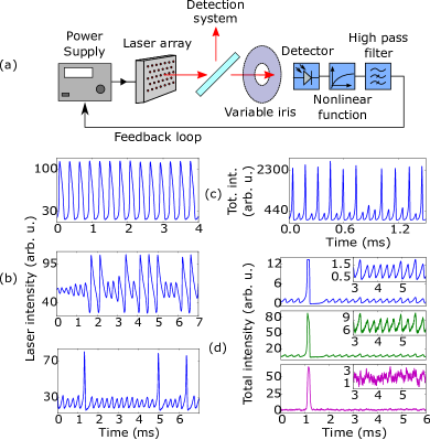
Figure 1: Experimental setup and typical dynamics. (a) The light emitted by an array of 451 lasers is converted to an electrical signal which, after filtering and nonlinear transformation, is reinjected into the single current source driving all lasers. (b) Single-laser time-traces showing: periodic oscillations, chaotic bursting and spiking (pumping currents 195.0 mA, 196.5 mA and 187.0 mA). (c) Mean-field time-trace of 451 lasers (182.1 mA), showing MMOs. (d) Top panel: total intensity of all 451 lasers, middle and bottom panels: intensity of two different lasers (pumping is 189.9 mA).

The experiment is shown on Fig. 1a). An array of 451 semiconductor lasers (Vertical Cavity Surface Emitting Lasers, VCSELs) is submitted to an AC-coupled nonlinear optoelectronic feedback. The dynamics of a single semiconductor laser can be described by two real coupled variables of widely differing time scales (light intensity, 10 ps, and semiconductor carrier population, 1 ns). As shown in Al-Naimee et al. (2009); Marino et al. (2011), chaotic spiking can arise via an incomplete homoclinic snaking scenario when a laser is driven close to its first (transcritical) bifurcation point and when an electric signal proportional to the intensity of the emitted field is reinjected back into the pumping current after a saturable nonlinear transformation and high-pass filtering. This signal constitutes a third (still much slower, typically 1 ms) variable. Due to the large pitch between the lasers there is no nearest neighbor coupling and the wavelength distribution of the lasers spans over 2 nm, preventing coherent interactions. All the lasers are driven by a single power supply, whose current is distributed evenly between all lasers (of identical impedance). The threshold current distribution is symmetric with average value 183.3 mA and standard deviation 5.8 mA. The emitted light is collected by a short focal length lens which forms an image of the array after about 10 cm propagation. Slightly before the image plane, the beam is split in two, one for detection and the other for the opto-electronic reinjection. In this beam, at the image plane, a variable aperture iris is used to control the sub-population which drives the dynamics. The light emitted by this population is converted by a photodetector into a voltage which is logarithmically amplified, providing a saturable nonlinearity. The continuous component is actively filtered out and the resulting signal is sent as a control voltage into the laser power supply. The aperture of the iris controls the coupling, from one to all to globally coupled. The control parameters are the driving current and the amount of light sent to the detector (controlled via a neutral density filter).

When the iris is closed to select a single laser, this device’s intensity drives the current applied to the whole population. The intensity of that particular laser can display complex dynamics as in Al-Naimee et al. (2009); Marino et al. (2011) including relaxation oscillations and chaotic bursting or spiking as shown in Fig. 1b). When the iris is completely open, the total intensity drives the power supply pumping the whole array, resulting in a mean-field coupled network of 451 nodes. Strikingly, the network can display periodic and chaotic mixed mode oscillations (MMOs) as shown in Fig. 1c). On Fig. 1d) we show synchronous measurements of the total intensity and of the intensity emitted by two different lasers in the mean-field coupled configuration during chaotic spiking: both lasers spike when the network spikes, but only one laser (central trace) displays the sub-threshold oscillations observed at the network level (top trace), while the other laser remains quiet (at the detection noise level, bottom trace).

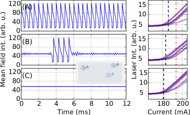
Figure 2: Dynamics of small networks. Different sub-populations (A, B and C) can be selected, showing different dynamics (left column). Each uncoupled population has a different laser threshold distribution (right column), the black dashed line shows the average threshold for each population (A:185.63 mA, B:182.88 mA, C:180.81 mA). The red dash-dotted line shows the constant current value used in all measurements (193.50 mA).

Smaller networks can be studied by partly closing the iris and detecting the corresponding population. Different dynamics are observed depending on the sub-population (Fig. 2). All parameters are constant and the amount of light sent to the detector is scaled to maintain the coupling constant when changing population. Each sub-population consists of seven elements whose threshold current differs slightly from device to device. Network A shows relaxation oscillations, B shows chaotic bursting and C is stationary. In all cases the dynamics of the total intensity seems low-dimensional. Each population is characterized by its threshold current distribution. The existence of a well-identified low-dimensional dynamics in populations of identical size but with distinct average threshold suggests that this parameter controls the dynamics.

The emergence of chaotic MMOs and of an effective, low-dimensional mean field dynamics can be inferred from the following. We consider a population of $N$ semiconductor lasers globally coupled through a common AC-coupled optoelectronic feedback. Each laser is modelled by standard single-mode rate equations describing the evolution of the optical intensity, carriers and feedback current. After proper scaling si , the equations read:

$$\dot{x_{i}} = x_{i}(y_{i}-1)\;$$ (1)

$$\dot{y_{i}} = \gamma(\delta_{i}-y_{i}+k(w+f(X))-x_{i}y_{i})\;$$ (2)

$$\dot{w} = -\epsilon(w+f(X))\;$$ (3)

where time has been normalized to the photon lifetime and $x_{i},y_{i}$ are respectively the dimensionless photon and carrier density of the laser $i$ and $X=\frac{1}{N}\sum\limits_{i=1}^{N}x_{i}$ is the total intensity normalized to the number of elements. The global variable $w$ is the (scaled) high-pass filtered feedback current, which includes a saturable nonlinear function $f(X)=A\ln(1+\alpha X)$. The optical and electrical propagation delays are negligible. All the lasers are considered identical except for the coherent emission threshold current that is included in the control parameter $\delta_{i}$ (proportional to the ratio between the common pump and the threshold current of each laser).

For $N=1$, there are two equilibria $(0,\delta_{1},0)$, $(\delta_{1}-1,1,-f(\delta_{1}-1))$. Since the normalized carrier rate $\gamma$ and AC feedback cutoff frequency $\epsilon$ are such that $\epsilon\ll\gamma\ll 1$, Eqs. (1-3) is a slow-fast system with three timescales. This model is strongly reminiscent of that of Al-Naimee et al. (2009, 2010); Marino et al. (2011). Similarly, the slow dynamics take place near a one-dimensional manifold $\Sigma=\Sigma_{x}\cup\Sigma_{y}$, where the lower attractive branch $\Sigma_{x}$ is given by the zero-intensity solution $\Sigma_{x}=\{x=0,y_{w}=\delta_{1}+kw,w\}$ while the middle repulsive and upper attracting branch, $\Sigma_{y}=\{x_{w},y=1,w\}$, is implicitly defined by the equation $\delta_{1}-1+kw+kf(x_{w})-x_{w}=0$. Since two branches rapidly attract all neighboring trajectories while the middle branch repels them, canard and relaxation cycles arise. These features are common in planar slow-fast systems but here a third intermediate time-scale, $1/\gamma$, induces more complex scenarios. First, the fixed points of the 2D fast subsystem (1-2) laying on the upper attractive critical branch consist of stable foci. Therefore the trajectories near these branches are shrinking helicoids, in contrast with the monotonic decay of the planar case. Second, a regime of regular or chaotic MMOs takes place, where canard orbits are separated by small-amplitude, quasi-harmonic oscillations surrounding the steady state of the system. When laying on the middle repelling branch, such equilibrium is a saddle focus and trajectories can rotate several times around it before switching to the other stable branch of the manifold. The number of these rotations, as well as the periodic or erratic nature of MMOs Desroches et al. (2012), are determined by the rates at which both $y_{1}$ and $w$ vary in the vicinity of the saddle-focus. This is related to the values of $\gamma$ and $\epsilon$, but also critically depends on the bifurcation parameter $\delta_{1}$.

When $N>1$, (1-3) describe a network of $N$ such elements, globally coupled through their slowest variable $w$. It admits $2^{N}$ equilibria which can be computed by splitting the population using the set $I$ of $N_{+}$ switched ON lasers with $(x_{i},y_{i})=(\delta_{i}-1,1),\ i\in I$ and the others $(x_{i},y_{i})=(0,\delta_{i}),\ i\notin I$ with $w=-f(\frac{1}{N}\sum\limits_{i\in I}\delta_{i}-\frac{N_{+}}{N})$. The stability of these equilibria can be computed as function of $\delta_{i}$ defining $\Delta=\frac{1}{N}\sum\limits_{i=1}^{N}\delta_{i}$ and assuming $\delta_{i}=\Delta+z\eta_{i},z\ll 1$, i.e. that the lasers are similar enough to each other si . At zero order in $z$, only the proportion $\frac{N_{+}}{N}$ of switched ON lasers affects the stability of the network which is otherwise determined by $\Delta$.

Figure 3: Numerical simulations of $10^{4}$ coupled lasers with optoelectronic feedback modelled by (1). Only the first 3 lasers dynamics are plotted (dashed and dotted lines). The mean dynamics is plotted in continuous black. The parameters $\frac{\delta_{i}-\left\langle\delta\right\rangle}{\left\langle\delta\right\rangle}$ are independent Gaussian variables of zero mean and standard deviation $1e-3$ with $\left\langle\delta\right\rangle=1.2045$, $k=0.7$, $A=1$, $\alpha=2$, $\gamma=4*10^{-3}$, $\epsilon=10^{-4}$. Black dot: intersection between the two slow manifold branches. The parabola $\Sigma_{y}$ and the straight line $\Sigma_{x}$ constitute the critical manifold calculated for a single laser with parameter $\Delta$.

Beyond stationary states, much insight can be gained by studying the stability of the critical manifold. Defining the mean carrier density $Y=\frac{1}{N}\sum\limits_{i=1}^{N}y_{i}$ we derive the following rate equations:

$$\dot{X} = -X+\frac{1}{N}\sum\limits_{i=1}^{N}x_{i}y_{i}\;$$ (4)

$$\dot{Y} = \gamma(\Delta-Y+k(w+f(X))-\frac{1}{N}\sum\limits_{i=1}^{N}x_{i}y_{i})\;$$ (5)

$$\dot{w} = -\epsilon(w+f(X)).\;$$ (6)

From Eq. 4, we have that $\dot{X}=0\Leftrightarrow X=\frac{1}{N}\sum\limits_{i=1}^{N}x_{i}y_{i}$. The critical manifold is solution of $\Delta-Y+kw+kf(X)-X=0$. It is clear that $\dot{X}=0$ is satisfied either if all lasers are off: $x_{i}=0$ $\forall i$, which gives $Y_{w}=\Delta+kw$ , or if all lasers are on: $y_{i}=1$ $\forall i$, so that $Y=1$. This provides two of the 1D branches of the critical manifold of the full network. These curves are defined by exactly the same equations as for $\Sigma$, but where all the variables and parameters are replaced by their corresponding mean values. To analyze the critical manifold in the general case, we parameterize it by the set $I$ of switched ON lasers and we introduce the new variable $X_{I}=\frac{1}{N}\sum\limits_{i\in I}x_{i}$ and parameter $\Delta_{I}=\frac{1}{N}\sum\limits_{i\in I}\delta_{i}$. We find that:

$$S_{I}=\{(x^{I}_{i}(w),y^{I}_{i}(w),w),\ i=1\cdots N,\ w\in\mathbb{R}\}$$

with

$$(x_{i}^{I}(w),y^{I}_{i}(w))=\left\{\begin{aligned} (0,\delta_{i}+k(w+f(X_{I}(w)))),&\quad\forall i\notin I,\\ (\delta_{i}-1+k(w+f(X_{I}(w))),1)&\quad\forall i\in I,\end{aligned}\right.$$

where $X_{I}(w)$ is implicitly defined by

$$X_{I}(w)=\frac{N_{+}}{N}(k(w+f(X_{I}(w)))-1)+\Delta_{I}.$$ (7)

The critical manifold of the mean-field coupled network thus consists of $2^{N}$ components: $S=\cup_{I\subset[1,N]}S_{I}$. Apart from the scaling factor $\frac{N_{+}}{N}$, the structure of the critical manifold is a bundle of 1D branches $S_{I}$ which, at zero order in $z$, closely resembles that of the $N=1$ case except for the OFF part. As for equilibria, the stability of $S_{I}$ can be determined analytically assuming that all lasers are similar enough $\delta_{i}=\Delta+z\eta_{i},z\ll 1$ si . It turns out that the stability of $S_{I}$, at zero order $z$, differs from that of a single ”mean” laser (with control parameter $\Delta$ and which incorporates the proportion $\frac{N_{+}}{N}$) by the destabilizing effect of the off part due to global coupling.

Figure 4: Bifurcation diagrams for the slow manifold of three networks of different sizes (D:19, E:251, F:451). Left: The dashed lines indicate the bifurcations from and to the only stable fixed point. Right: transcritical laser bifurcation curves for the uncoupled elements, the dashed line indicates the ensemble average of the threshold current values $\langle I_{th}\rangle$.

Thus, as the quenched disorder $\delta_{i}$ is not averaged in the limit $N\to\infty$, a truly mean field limit cannot be established as an ODE. However, due to the splitting of the timescales, most of the motion takes place along the critical manifold leading to an effective low dimensional dynamics very similar to that of a single element. In Fig. 3, we plot the numerical mean field trajectory together with the critical manifold of an average laser. The slow evolution of different nodes is perfectly synchronized, even if some elements may be on different branches of the slow manifold (as in the experimental observation of Fig. 1 d)). However, the individual trajectories differ in the fast part of the dynamics, which is transversal to the slow manifold. This is clear on the bottom of Fig. 3 which shows a time trace of the mean field together with the variance of the $x_{i}$. In absence of noise, the distribution of the $x_{i}$ tendis to a Dirac function whenever the system is close to the critical manifold with a much broader distribution when the system switches branch.

Finally, the dynamics for $z\ll 1,N<\infty$ stays in a tube around the dynamics for $z=0$ in which case there is no disorder and thus the dynamics is exactly that of the isolated laser. This implies that the MMO and the chaotic behaviors (for $z=0$) are robust on finite time intervals when $N$ grows to infinity. This is exemplified in Fig. 3 which shows a chaotic trajectory in the case $z\ll 1,N=10^{4}$.

We assess the impact of $\Delta$ experimentally by measuring the total intensity for different population sizes (Fig. 4). All parameters are constant and the iris is opened to include a larger and larger population. For each network size, the total amount of light sent to the reinjection detector is scaled to keep the coupling parameter constant. We show the bifurcation diagrams of networks of 19 (D), 251 (E) and 451 (F) nodes on Fig. 4. Similar sequences are observed, although for different values of the control parameter. The distributions of the uncoupled laser emission thresholds are shown on the right column. The 451 and 251 elements networks are very similar but the 19 element one differs markedly. As expected from theory, this hints at $\Delta$ as control parameter for the network.

We demonstrate this convergence by measuring the current value at which some prescribed dynamics takes place for different populations. On Fig. 5, we plot the current value $\mathcal{I}_{s}$ at which the network returns to a stable fixed point after undergoing the sequence of bifurcations described earlier, as a function of the average threshold current of the sub-population. The size and color of each marker indicate the size of the network. The error bars are estimates of the measurement error. Smaller networks are disperse but larger networks converge towards the same point in this $(<I_{th}>,\mathcal{I}_{s})$ space. The dispersion of the measurements around a straight line results from the scaling of the bifurcation parameter $\Delta=\frac{I_{0}-I_{t}}{<I_{th}>-I_{t}}$ where $I_{t}$ is the transparency current (assumed to be equal for all devices).

Figure 5: Upper bifurcation parameter value depending on average laser threshold value for increasing sample size. Smaller samples (lighter blue) are distributed along a straight line. When the sample grows (darker blue) the bifurcation parameter converges to a well defined value. Inset: convergence of the empirical mean towards its final value for the largest population and fit in $1/\sqrt{N}$.

Summarizing, we have reported experimental observations of mixed mode oscillations and spiking in a mean field coupled network of hundreds of semiconductor lasers chaotically spiking and coupled through nonlinear optoelectronic feedback. A transport equation for the probability density $p(t,x,y,w,\delta)$ of the limit laser for $N\longrightarrow\infty$ involves the full distribution of the $\delta_{i}$, which shows that the mean field cannot be described with an ODE. These phenomena result from the slow-fast nature of the system. Through the stability analysis of the critical manifold, we demonstrate that the network experiences an effectively low-dimensional dynamics even when the fast dynamics of the nodes is not synchronized. These experimental observations show that the results are robust with respect to some amount of disorder in the couplings. Thanks to the relative simplicity of the experimental platform, we expect that the present results open several research avenues, specifically on the role of noise in coupled slow-fast systems and on networks of networks.