GPU-based parallelism for ASP-solving 

Abstract

Answer Set Programming (ASP) has become, the paradigm of choice in the field of logic programming and non-monotonic reasoning. Thanks to the availability of efficient solvers, ASP has been successfully employed in a large number of application domains. The term GPU-computing indicates a recent programming paradigm aimed at enabling the use of modern parallel Graphical Processing Units (GPUs) for general purpose computing. In this paper we describe an approach to ASP-solving that exploits GPU parallelism. The design of a GPU-based solver poses various challenges due to the peculiarities of GPUs’ software and hardware architectures and to the intrinsic nature of the satisfiability problem. SP solvers, ASP computation, SIMT parallelism, GPU computing

Introduction

Answer Set Programming (ASP) is an expressive and purely declarative framework developed in the last decades in the Logic Programming and Knowledge Representation communities. Thanks to its extensively studied mathematical foundations and the continuous improvement of efficient and competitive solvers, ASP has become the paradigm of choice in many fields of AI. It has been fruitfully employed in many areas, such as knowledge representation and reasoning, planning, bioinformatics, multi-agent systems, data integration, language processing, declarative problem solving, semantic web, robotics, to mention a few among many [7, 8].

The clear and highly declarative nature of ASP enables excellent opportunities for the introduction of parallelism and concurrency in implementations of ASP-solvers. Steps have been made in the last decade toward the parallelization of the basic components of Logic Programming systems. Implementations of solvers exploiting multicore architectures, distributed systems, or portfolio approaches, have been proposed [4]. In this direction, a recent new stream of research concerns the design and development of parallel ASP systems that can take advantage of the massive degree of parallelism offered by modern Graphical Processing Units (GPUs).

GPUs are multicore devices designed to operate with very large number of lightweight threads, executing in a rigid synchronous manner. They present a significantly complex memory organization. To take full advantage of GPUs’ computational power, one has to adhere to specific programming directives, in order to proficiently distribute the workload among the computing units and achieve the highest throughput in memory accesses. This makes the model of parallelization used on GPUs deeply different from those employed in more “conventional” parallel architectures. For these reasons, existing parallel solutions are not directly applicable in the context of GPUs.

This paper illustrates the design and implementation of a conflict-driven ASP-solver that is capable of exploiting the Single-Instruction Multiple-Thread parallelism offered by GPUs. As we will see, the overall structure of the GPU-based solver is reminiscent of the conventional structure of sequential conflict-driven ASP solvers (such as, for example, the state-of-the-art solver clasp [11]). However, substantial differences lay in both the implemented algorithms and in the adopted programming model. Moreover, we avoid two hardly parallelizable and intrinsically sequential components usually present in existing solvers. On the one hand, we exploit ASP computations to avoid the introduction of loop formulas and the need of performing unfounded set checks [11]. On the other hand, we adopt a parallel conflict analysis procedure as an alternative to the sequential resolution-based technique used in clasp.

The paper is organized as follows. Sect. 1 recalls basic notions on ASP, GPU-computing, and the CUDA framework. The approach to ASP solving based on conflict-driven nogood learning is described in Sect. 2. Sect. 3 illustrates the difficulties inherent in parallelizing irregular applications, such as ASP, on GPUs. The software architecture of the CUDA-based ASP-solver yasmin is outlined in Sect. 4. In particular, the new parallel learning procedure is presented in Sect. 4.2 and evaluated in Sect. 5.

1 Preliminaries

We briefly recall the basic notions on ASP needed in the rest of the paper (for a detailed treatment see [12, 11] and the references therein). Similarly, we also recall few needed notions on CUDA parallelism [17, 18].

Answer Set Programming. 

An ASP program $\Pi$ is a set of ASP rules of the form:

$p_{0}\leftarrow p_{1},\dots,p_{m},\textit{not }p_{m+1},\dots,\textit{not }p_{n}$

where $n\geq 0$ and each $p_{i}$ is an atom. If $n=0$, the rule is a fact. If $p_{0}$ is missing, the rule is a constraint. Notice that such a constraint can be rewritten as a headed rule of the form $q\leftarrow p_{1},\dots,p_{m},\textit{not }p_{m+1},\dots,\textit{not }p_{n},\textit{not }q$, where $q$ is a fresh atom. Hence, constraints do not increase the expressive power of ASP.

A rule including variables is simply seen as a shorthand for the set of its ground instances. Without loss of generality, in what follows we consider the case of ground programs only. (Hence, each $p_{i}$ is a propositional atom.)

Given a rule $r$, $p_{0}$ is referred to as the head of the rule ($head(r)$), while the set $\{p_{1},\dots,p_{m},\textit{not }p_{m+1},\dots,\textit{not }p_{n}\}$ is referred to as the body of $r$ ($body(r)$). Moreover, we put $body^{+}(r)=\{p_{1},\dots,p_{m}\}$, $body^{-}(r)=\{p_{m+1},\dots,p_{n}\}$, $\varphi^{+}(r)=p_{1}\wedge\dots\wedge p_{m}$ and $\varphi^{-}(r)=\neg p_{m+1}\wedge\dots\wedge\neg p_{n}$. We will denote the set of all atoms in $\Pi$ by $atoms(\Pi)$ and the set of all rules defining the atom $p$ by $rules(p)=\{{r}\mid{head(r)=p}\}$. The completion $\Pi_{cc}$ of a program $\Pi$ is defined as the formula:

$\Pi_{cc}=\bigwedge_{p\in atoms(\Pi)}\Big{(}p~{}\leftrightarrow~{}\bigvee_{r\in rules(p)}\big{(}\varphi^{+}(r)\wedge\varphi^{-}(r)\big{)}\Big{)}$.

Semantics of ASP programs is expressed in terms of answer sets. An interpretation is a set $M$ of atoms; $p\in M$ (resp. $p\not\in M$) denotes that $p$ is true (resp. false). An interpretation is a model of a rule $r$ if $head(r)\in M$, or $body^{+}(r)\setminus M\neq\emptyset$, or $body^{-}(r)\cap M\neq\emptyset$. $M$ is a model of a program $\Pi$ if it is a model of each rule in $\Pi$. $M$ is an answer set of $\Pi$ if it is the subset-minimal model of the reduct program $\Pi^{M}$.

An important connection exists between the answer sets of $\Pi$ and the minimal models of $\Pi_{cc}$. In fact, any answer set of $\Pi$ is a minimal model of $\Pi_{cc}$. The converse is not true, but it can be shown [14] that the answer sets of $\Pi$ are the minimal models of $\Pi_{cc}$ satisfying the loop formulas of $\Pi$. The number of loop formulas can be, in general, exponential in the size of $\Pi$. Hence, modern ASP solvers adopt some form of lazy approach to generate loop formulas only “when needed”. We refer the reader to [14, 11] for the details; in what follows we will describe an alternative approach to answer set computation that avoids the generation of loop formulas. The new approach exploits ASP computations to avoid the introduction of loop formulas and the need of performing unfounded set checks [11] during the search of answer sets.

The notion of ASP computations originates from a computation-based characterization of answer sets [15] based on an incremental construction process, where at each step choices determine which rules are actually applied to extend the partial answer set. More specifically, for a program $\Pi$ let $T_{\Pi}$ be the immediate consequence operator of $\Pi$. Namely, if $I$ is an interpretation, then

$T_{\Pi}(I)=\big{\{}{head(r)}\,\mid\,r\in\Pi\,\wedge body^{+}(r)\subseteq I\wedge body^{+}(r)\cap I=\emptyset\big{\}}$.

An ASP Computation for $\Pi$ is a sequence of interpretations $I_{0},I_{1},I_{2},\dots$ (where $I_{0}$ can be any set of atoms that are logical consequences of $\Pi$) satisfying these conditions:

• $I_{i}\subseteq I_{i+1}$ for all $i\geq 0$

• $I_{\infty}=\bigcup_{i=0}^{\infty}I_{i}$ is such that $T_{\Pi}(I_{\infty})=I_{\infty}$;

• $I_{i+1}\subseteq T_{\Pi}(I_{i})$ for all $i\geq 0$;

• if $p\in I_{i+1}\setminus I_{i}$ then there is $r\in rules(p)$ such that $I_{j}$ is a model of $body(r)$ for each $j\geq i$.

Following [15], an interpretation $I$ is an answer set of $\Pi$ if and only if there exists an ASP computation such that $I=\bigcup_{i=0}^{\infty}I_{i}$.

GPU-computing and the CUDA framework.

Graphical Processing Units (GPUs) are massively parallel devices, originally developed to support efficient computer graphics and fast image processing. The use of such multicore systems has become pervasive in general-purpose applications that are not directly related to computer graphics, but demand massive computational power. The term GPU-computing indicates the use of the modern GPUs for such general-purpose computing. NVIDIA is one of the pioneering manufacturers in promoting GPU-computing, especially through the support to its Computing Unified Device Architecture (CUDA) [18]. A GPU contains hundreds or thousands of identical computing units (cores) and provides access to both on-chip memory (used for registers and shared memory) and off-chip memory (used for cache and global memory). Cores are grouped in a collection of Streaming MultiProcessors (SMs); in turn, each SM contains a fixed number of computing cores.

The underlying conceptual model for parallelism is Single-Instruction Multiple-Thread (SIMT), where the same instruction is executed by different threads that run on cores, while data and operands may differ from thread to thread. A logical view of computations is introduced by CUDA, in order to define abstract parallel work and to schedule it among different hardware configurations. A typical CUDA program is a C/C++ program that includes parts meant for execution on the CPU (referred to as the host) and parts meant for parallel execution on the GPU (referred to as the device).

The CUDA API supports interaction, synchronization, and communication between host and device. Each device computation is described as a collection of concurrent threads, each executing the same device function (called a kernel, in CUDA terminology). These threads are hierarchically organized in blocks of threads and grids of blocks. The host program contains all the instructions needed to initialize the data in the GPU, specify the number of grids/blocks/threads, and manage the kernels. Each thread in a block executes an instance of the kernel, and has a thread ID within its block. A grid is a 3D array of blocks that execute the same kernel, read data input from the global memory, and write results to the global memory. When a CUDA program on the host launches a kernel, the blocks of the grid are scheduled to the SMs with available execution capacity. The threads in the same block can share data, using high-throughput on-chip shared memory, while threads belonging to different blocks can only share data through the global memory. Thus, the block size allows the programmer to define the granularity of threads cooperation.

It should be noticed that the most efficient access pattern to be adopted by threads in reading/storing data depends on the kind of memory. We briefly mention here two possibilities (see [17] for a comprehensive description). Shared memory is organized in banks. In case threads of the same block accesses locations in the same bank, a bank conflict occurs and the accesses are serialized. To avoid bank conflicts, strided access pattern has to be adopted. On the contrary, concerning global memory, to reach the highest throughput, coalesced accesses have to be executed. Intuitively, this can be achieved if consecutive threads access contiguous global memory locations.

Threads of each block are grouped in warps of 32 threads each. The threads of the same warp share the fetch of the instruction code to be executed. Hence, the maximum efficiency is achieved when all 32 threads execute the same instruction (possibly, on different data). Whenever two (or more) groups of threads belonging to the same warp fetch/execute different instructions, thread divergence occurs. In this case the execution of the different groups is serialized and the overall performance decreases.

A simple CUDA application presents the following basic components:

• Before being processed by kernels, data must be copied to the global memory of the device. The CUDA API supports memory allocation and data transfer to/from the host.

• Kernels are defined as standard C functions; the annotation used to communicate to the CUDA compiler that a function should be treated as kernel has the form:  __global__ void kernelName (Formal Arguments).

• A kernel can be launched from the host program using:
  

  kernelName <<< GridDim, TPB >>> (Actual Arguments)

  where GridDim describes the number of blocks of the grid and TPB specifies the number of threads in each block.

• After the execution of the kernel, the host retrieves the results with a transfer operation from global memory to host memory.

2 Conflict-driven ASP-Solving

Conflict-driven nogood learning (CDNL) is one of the techniques successfully used by ASP-solvers, such as the clingo system [11]. The first attempt in exploiting GPU parallelism for conflict-driven ASP solving has been made in [5, 6]. The approach adopts a conventional architecture of an ASP solver which starts by translating the completion $\Pi_{cc}$ of a given ground program $\Pi$ into a collection of nogoods (see below). Then, the search for the answer sets of $\Pi$ is performed by exploring a search space composed of all interpretations for the atoms in $\Pi$, organized as a binary tree. Branches of the tree correspond to (partial) assignments of truth values to program atoms (i.e., partial interpretations). The computation of an answer set proceeds by alternating decision steps and propagation phases. Intuitively: (1) A decision consists in selecting an atom and assigning it a truth value. (This step is usually guided by powerful heuristics analogous to those developed for SAT [2].) (2) Propagation extends the current partial assignment by adding all consequences of the decision. The process repeats until a model is found (if any). It may be the case that inconsistent truth values are propagated for the same atom after $i$ decisions (i.e., while visiting a node at depth $i$ in the tree-shaped search space). In such cases a conflict arises at decision level $i$ testifying that the current partial assignment cannot be extended to a model of the program. Then, a conflict analysis procedure is run to detect the reasons of the failure. The analysis identifies which decisions should be undone in order to restore consistency of the assignment. It also produces a new learned nogood to be added to the program at hand, so as to exclude repeating the same failing sequence of decisions, in the subsequent part of the computation. Consequently, the program is extended with the learned nogood and the search backjumps to a previous (consistent) point in the search space, at a decision level $j<i$. Whenever a conflict occurs at the top decision level ($i=1$), the computation ends because no (more) solutions exist.

Following [5, 6], let us outline how CDNL can be combined with ASP computation in order to obtain a solver that does not need to use loop formulas. We describe both assignments $A$ and nogoods $\delta$ as sets of signed atoms—i.e., entities of the form $Tp$ or $Fp$, denoting that $p\in atoms(\Pi)$ has been assigned true or false, respectively. Plainly, assignment contains at most one element between $Tp$ and $Fp$ for each atom $p$. Given an assignment $A$, let $A^{T}=\{{p}\mid{Tp\in A}\}$. Note that $A^{T}$ is an interpretation for $\Pi$. A total assignment $A$ is such that, for every atom $p$, $\{Tp,Fp\}\cap A\neq\emptyset$. Given a (possibly partial) assignment $A$ and a nogood $\delta$, we say that $\delta$ is violated if $\delta\subseteq A$. In turn, $A$ is a solution for a set of nogoods $\Delta$ if no $\delta\in\Delta$ is violated by $A$. Nogoods can be used to perform deterministic propagation (unit propagation) and extend an assignment. Given a nogood $\delta$ and a partial assignment $A$ such that $\delta\setminus A=\{Fp\}$ (resp., $\delta\setminus A=\{Tp\}$), then we can infer the need to add $Tp$ (resp., $Fp$) to $A$ in order to avoid violation of $\delta$.

Given a program $\Pi$, a set of completion nogoods $\Delta_{\Pi_{cc}}$ is derived from $\Pi_{cc}$ as follows. For each rule $r\in\Pi$ and each atom $p\in atoms(\Pi)$, we introduce the formulas:

$\begin{array}[]{rcl c rcl c rcl c rcl}b_{r}&\leftrightarrow&t_{r}\wedge n_{r}&{}{}{}{}{}\hfil&t_{r}&\leftrightarrow&\varphi^{+}(r)&{}{}{}{}{}\hfil&n_{r}&\leftrightarrow&\varphi^{-}(r)&{}{}{}{}{}\hfil&p&\leftrightarrow&\bigvee_{r\in rules(p)}b_{r}\\ \end{array}$

where $b_{r},t_{r},n_{r}$ are new atoms (if $rules(p)=\emptyset$, then the last formula reduces to $\neg p$). The completion nogoods reflect the structure of the implications in these formulas:

• from the first formula we have the nogoods: $\{Fb_{r},Tt_{r},Tn_{r}\},\{Tb_{r},Ft_{r}\}$, and $\{Tb_{r},Fn_{r}\}$.

• From the second and third formulas we have the nogoods: $\{Tt_{r},Fp\}$ for each $p\in body^{+}(r)$; $\{Tn_{r},Tq\}$ for each $q\in body^{-}(r)$; $\{Ft_{r}\}\cup\{{Tp}\mid{p\in body^{+}(r)}\}$; and $\{Fn_{r}\}\cup\{{Fq}\mid{q\in body^{-}(r)}\}$.

• From the last formula we have the nogoods: $\{Fp,Tb_{r}\}$ for each $r\in rules(p)$ and $\{Tp\}\cup\{{Fb_{r}}\mid{r\in rules(p)}\}$.

Moreover, for each constraint $\leftarrow p_{1},\dots,p_{m},\textit{not }p_{m+1},\dots,\textit{not }p_{n}$ in $\Pi$ we introduce a constraint nogood of the form $\{Tp_{1},\dots,Tp_{m},Fp_{m+1},\dots,Fp_{n}\}$. The set $\Delta_{\Pi_{cc}}$ is the set of all the nogoods so defined.

The basic CDNL procedure described earlier can be easily combined with the notion of ASP computation. Indeed, it suffices to apply a specific heuristic during the selection steps to satisfy the four properties defined in Sect. 1. This can be achieved by assigning true value to a selected atom only if this atom is supported by a rule with true body. More specifically, let $A$ be the current partial assignment, the selection step acts as follows. For each unassigned atom $p$ occurring as head of a rule in the original program, all nogoods reflecting the rule $b_{r}\leftarrow t_{r},n_{r}$, such that $r\in rules(p)$ are analyzed to check whether $Tt_{r}\in A$ and $Fn_{r}\notin A$ (i.e., the rule is applicable [15]). One of the rules $r$ that pass this test is selected. Then, $Tb_{r}$ is added to $A$. In the subsequent propagation phase $Tp$ and $Fn_{r}$ are also added to $A$ and $Fn_{r}$ imposes that all the atoms of $body^{-}(r)$ are set to false. This, in particular, ensures the persistence of beliefs of the ASP computation. (In the real implementation (see Sect. 4) all applicable rules $r$, and their heads, are evaluated according to a heuristic weight and the rule $r$ with highest ranking is selected.) It might be the case that no selection is possible because no unassigned atom $p$ exists such that there is an applicable $r\in rules(p)$. In this situation the computation ends by assigning false value to all unassigned heads in $\Pi$. This completes the assignment, which is validated by a final propagation step in order to check that no constraint nogoods are violated. In the positive case the assignment so obtained is an answer set of $\Pi$.

3 ASP as an irregular application

The design of GPU-based ASP-solvers poses various challenges due to the structure and intrinsic nature of the satisfiability problem. The same holds for GPU-based approaches to SAT [3]. As a matter of fact, the parallelization of SAT/ASP-solving shares many aspect with other applications of GPU-computing where problems/instances are characterized by the presence of large, sparse, and unstructured data. Parallel graph algorithms constitute significant examples, that, like SAT/ASP solving, exhibit irregular and low-arithmetic intensity combined with data-dependent control flow and memory access patterns. Typically, in these contexts, large instances/graphs have to be modeled and represented using sparse data structures (e.g., matrices in Compressed Sparse Row/Column formats). The parallelization of such algorithms struggle to achieve scalability due to lack of data locality, irregular access patterns, and unpredictable computation [16]. Although, in the case of some graph algorithms, several techniques have been established in order to improve performance on parallel architectures [13] and accelerators [1], the different character of the algorithms used in SAT/ASP might prevent from obtaining comparable impact on performance by directly applying the same techniques. This is because, first, the time-to-solution of a SAT/ASP problem is dominated by heuristic selection and learning procedures able to cut the exponential search space. In several cases, smart heuristics might be most effective than advanced parallel solutions. Second, because of intrinsic data-dependencies, procedures like propagation or learning often require to access large parts of the data/graph, sequentially. Similarly to what experienced in other complex graph-based problems [9], the kind of computation involved differs from that of traversal-like algorithms (such as, Breadth-First Search) which process a subset of the graph in iterative/incremental manners and for which advanced GPU-solutions exist. Furthermore, aspect specific to the underlying architecture enters into play, such as coalesced memory access and CUDA-thread balancing, which are major objectives in parallel algorithm design. In this scenario, our GPU-based proposal to ASP solving also implements:

• efficient parallel propagation able to maximize memory throughput and minimize thread divergence.

• Fast parallel learning algorithm which avoids the bottleneck represented by the intrinsically sequential resolution-like learning procedures commonly used in CDNL solvers.

• Specific thread-data mapping solutions able to regularize the access to data stored in global, local, and shared memories.

In what follows we will describe how to achieve these requirements in the GPU-based solver for ASP.

procedure yasmin($\Delta$: SetOfNogoods, $P$: GroundProgram)

1 $cdl\leftarrow 1$ ;  reset ($A$)

  /* set initial decision level and empty assignment */

2 $\textnormal{{InitialPropagation}}\texttt{<<<b,t>>>}(A,\Delta,\mathit{Viol})$ /* check input units satisfaction */

3 if $\mathit{Viol}$ then return no-answer-set

4 else loop  

      5 $\textnormal{{PropagateAndCheck}}(A,\Delta,cdl,\mathit{Viol})$

        /* update $A$ and flag $Viol$ */

      6 if $\mathit{Viol}\land(cdl=1)$ then return no-answer-set

      7  /* Violation at first dec.level */ else if $\mathit{Viol}$ then /* Violation at level $cdl{>}1$ */

            8 $\textnormal{{Learning}}\texttt{<<<b,t>>>}(\Delta,A,cdl)$

              /* conflict analysis: update $\Delta$ and $cdl$ */

            9 $\textnormal{{Backjump}}\texttt{<<<b,t>>>}(A,cdl)$

              /* update $A$ and $cdl$ */

            

       end if

      10if ($A$ is not total) then

             /* rank selectable literals and applicable rules. If possible, select $Lit$, extend $A$, update $cdl$. Otherwise, $Lit\leftarrow\mathit{nil}$ : */

            11 $\textnormal{{Decision}}\texttt{<<<b,t>>>}(\Delta,A,\mathit{Lit})$

            12 if $\mathit{Lit}=\mathit{nil}$ then /* no applicable rules */

                  13 $\textnormal{{CompleteAssignment}}\texttt{<<<b,t>>>}(A)$ /* falsify unassigned atoms */

            

      14 else return $A^{T}\cap atom(P)$ /* stable model found */

      

Algorithm 1 Host code of the ASP-solver yasmin     (simplified)

4 The CUDA-based ASP-solver yasmin

In this section, we present a solver that exploits ASP computation, nogoods handling, and GPU parallelism. The ground program $\Pi$, as produced by the grounder gringo [11], is read by the CPU. The CPU also computes the completion nogoods $\Delta_{\Pi_{cc}}$ and transfers them to the device. The rest of the computation is performed completely on the GPU. During this process, there only memory transfers between the host and device involve control-flow flags (e.g., an “exit” flag, used to communicate whether the computation is terminated) and the computed answer set (from the GPU to the CPU).

As concerns representation and storing of data on the device, nogoods are represented using Compressed Sparse Row (CSR) format. The atoms of each nogood are stored contiguously and all nogoods are stored in consecutive locations of an array allocated in global memory. An indexing array contains the offset of each nogood, to enable direct accesses to them. (Such indexes are then used as identifiers for the corresponding nogoods.) Nogoods are sorted in increasing order, depending on their length. Each atom in $\Pi$ is uniquely identified by an index, say $p$. A array $A$ of integers is used to store in global memory the set of assigned atoms (with their truth values) in this manner:

• $A[p]=0$ if and only if the atom $p$ is unassigned;

• $A[p]=i$, $i>0$ (resp., $A[p]=-i$) means that atom $p$ has been assigned true (resp., false) at the decision level $i$.

The basic structure of the yasmin solver is shown in Alg. 1. We adopt the following notation: for each signed atom $p$, let $\overline{p}$ represent the same atom with opposite sign. Moreover, let us refer to the stored set of nogoods simply by the variable $\Delta$. The variable $cdl$ (initialized in line 1) represents the current decision level. As mentioned, $cdl$ acts as a counter that keeps track of the current number of decisions that have been made.

Since the set of input nogoods may include some unitary nogoods, a preliminary parallel computation partially initializes $A$ accordingly (line 2). It may be the case that inconsistent assignments occur in this phase. In such case a flag $Viol$ is set, the given program $\Pi$ in declared unsatisfiable (line 3) and the computation ends. Notice that the algorithm can be restarted several times—typically, this happens when more than one solution is requested or if restart strategy is activated by command-line options. (For simplicity, we did not include the code for restarting the solver in Alg. 1.) In such cases, InitialPropagation() also handles unit nogoods that have been learned in the previous execution. The kernel invocation in line 2 specifies a grid of b blocks each composed of t threads. The mapping is one-to-one between threads and unitary nogood. In particular, if $k$ is the number of unitary nogoods, b=$\lceil k/TPB\rceil$ and t=$TPB$, where $TPB$ is the number of threads-per-block specified via command-line option. The loop in lines 4–14 computes the answer set, if any. Propagation is performed by the procedure PropagateAndCheck() in line 5, which also checks whether nogood violations occur. To better exploit the SIMT parallelism and maximize the number of concurrently active threads, in each device computation the workload has to be divided among the threads of the grid as uniformly as possible. To this aim, PropagateAndCheck() launches multiple kernels: one kernel deals with all nogoods with exactly two literals; a second one processes the nogoods composed of three literals, and a further kernel processes all remaining nogoods. In this manner, threads of the same grid process a uniform number of atoms, reducing the divergence between them and minimizing the number of inactive threads. Moreover, because, as mentioned, nogoods of the same length are stored contiguously, threads of the same grid are expected to realize coalesced accesses to global memory. A more detailed description of the third of such device functions is given in Sect. 4.1. A similar technique is used in PropagateAndCheck() to process those nogoods that are learned at run-time through the conflict analysis step (cf. Sect. 4.2). These nogoods are partitioned depending on their cardinality and processed by different kernels, accordingly. In general, if $n$ is the number of nogoods of one partition, the corresponding kernel has b=$\lceil n/TPB\rceil$ blocks of t=$TPB$ threads each. Each thread processes one learned nogood.

Propagation stops because either a fixpoint is reached (no more propagations are possible) or one or more conflicts occur. In the latter case, if the current decision level is the top one the solver ends: no solution exists (line 6). Otherwise, (lines 7–9) conflict analysis (Learning()) is performed and then the solver backjumps to a previous decision point (line 9). The learning procedure is describes in Sect. 4.2. A specific kernel Backjump() takes care of updating the value of $cdl$ and the array that stores the assignment. A mapping one-to-one between threads and atoms in $A$ is used.

On the other hand, if no conflict occurs and $A$ is not complete, a new Decision() is made (line 11). As mentioned, the purpose of this kernel is to determine an unassigned atom $p$ which is head of an applicable rule $r$. All candidates $p$ and applicable $r$ are evaluated in parallel according to a typical heuristics to rank the atoms. Possible criteria, selectable by command-line options, use the number of positive/negative occurrences of atoms in the program (by either simply counting the occurrences or by applying the Jeroslow-Wang heuristics) or the “activity” of atoms [2]. The first access to global memory to retrieve needed data is done in coalesced manner (a mapping one-to-one between threads and rules is used). Then, a logarithmic parallel reduction scheme, implemented using thread-shuffling to avoid further accesses to global memory, yields the rule $r$ with highest ranking. Its head is selected and set true in the assignment. Decision() also communicates to the solver whether no applicable rule exists (line 12). In this case all unassigned heads in $\Pi$ are assigned false (by the kernel CompleteAssignment() in line 13). A successive invocation of PropagateAndCheck() validates the answer set and the solver ends in line 14.

4.1 The propagate-and-check procedure

After each assignment of an atom of the current partial assignment $A$, each nogood $\delta$ needs to be analyzed to detect whether: (1) it is violated, or (2) there is exactly one literal $p$ in it that is unassigned in $A$, in which case an inference step adds $\overline{p}$ to $A$ (cf., Sect. 2). The procedure is repeated until a fixpoint is reached. As seen earlier, this task is performed by the kernels launched by the procedure PropagateAndCheck().

Alg. 2 shows the device code of the generic kernel dealing with nogoods of length greater than three (the others are simpler). The execution of each iteration is driven by the atoms that have been assigned a truth value in the previous iteration (array $Last$ in Alg. 2). Thus, each kernels involves a number of blocks that is equal to the number of such assigned atoms. The threads in each block process the nogoods that share the same assigned atom. The number of threads of each block is established by considering the number of occurrences of each assigned atom in the input nogoods. Observe that the dimension of the grid may change between two consecutive invocations of the same kernel, and, as such, it is evaluated each time. Specific data structures (initialized once during a pre-processing phase and stored in the sparse matrix $\mathit{Map[][]}$ in Alg. 2) are used in order to determine, after each iteration and for each assigned atom, which are the input nogoods to be considered. A further technique is adopted to improve performance. Namely, the processing of nogoods is realized by implementing a standard technique based on watched literals [2]. In this case, each thread accesses the watched literals of a nogood and acts accordingly. The combination of nogood sorting and the use of watched literals, improves the workload balancing among threads and mitigates thread divergence. (Watched literals are exploited also for long learned nogoods.)

Concerning Alg. 2, each thread of the grid first retrieves one of the atoms propagated during the previous step (line 1). Threads of the same block obtain the same atom $L$. In line 2, threads accesses the data structure $Maps$, mentioned earlier, to retrieve the number $ngInBlock$ of nogoods to be processed by the block. In line 5 each thread of the block determines which nogood has to be processed and retrieves its watched literals (lines 6-7). In case one or both literals belongs to the current assignment $A$, suitable substitutes are sought for (lines 10 and 14). Violation might be detected (lines 12 and 19, resp.) or propagation might occur (lines 16–18). Notice that, concurrent threads might try to propagate the same atom (possibly with different sign), originating race conditions. The use of atomic functions (line 16) allows one nondeterministically chosen thread $t$ to perform the propagation. Other threads may discover agreement or detect inconsistency w.r.t. the value set by $t$ (line 19). In line 17 the thread $t$ updates the set $Next$ of propagated atoms (to be used in the subsequent iteration) and stores (line 18) information needed in future conflict analysis steps (by means of mk_dl_bitmap(), to be described in Sect. 4.2) and concerning the causes of the propagation.

procedure nogood_check($\mathit{Last}$, $\mathit{Next}$ : ArrayOfLits, $\mathit{Map}$ : AtomsNogoodsMatrix, $A$: Assignment)

1 $L\leftarrow\mathit{Last}[blockIdx.x]$ /* each block processes one of the propagated lits */

2 $\mathit{ngInBlock}\leftarrow~{}|\mathit{Map}[L]|$ /* get the number of nogoods in which $L$ occurs */

3 $i\leftarrow\mathit{threadIdx}.x$ /* each nogood in which $L$ occurs is treated by a thread */

4 if $i<\mathit{ngInBlock}$ then

      5 $\delta\leftarrow\mathit{Map}[L][i]$ /* get the nogood */

      6 $w_{1}\leftarrow\mathit{watched}_{1}[\delta]$ /* copy the two watched lits in registers */

      7 $w_{2}\leftarrow\mathit{watched}_{2}[\delta]$

      8 if $\overline{w_{1}}\in A\vee\overline{w_{2}}\in A$ then return

      9  /* satisfied nogood, thread exits */ if $w_{1}\in A\wedge w_{2}\in A$ then

            10 if exists $w\in\delta$ such that $w\not\in A\wedge\overline{w}\not\in A$ then

                  11 $w_{1}\leftarrow w$

            12else  $Viol\leftarrow true$

              /* nogood violation */

      13 if $w_{1}\not\in A\wedge w_{2}\in A$ then /* the case $w_{2}\not\in A\wedge w_{1}\in A$ is analogous (omitted) */

            14 if exists $u\in\delta$ such that $w_{1}\not=u\wedge u\not\in A\wedge\overline{u}\not\in A$ then

                  15 $w_{2}\leftarrow u$

             else  /* first thread propagates (others may agree or cause violation) */

                  16 if $atomicSet(A,w_{1},cdl)$ then /* returns true if found not disagreeing */

                        17 $\mathit{Next}\leftarrow\mathit{Next}\cup\{w_{1}\}$ /* update set of propagated lits */

                        18 $\mathit{Deps}[w_{1}]=\textnormal{{mk\_dl\_bitmap}}(w_{1},\delta)$ /* set dependencies of $w_{1}$ */

                        

                  19else  $Viol\leftarrow true$

                    /* if disagreeing, it is a violation */

            

      20 $\mathit{watched}_{1}[\delta]\leftarrow w_{1}$  ;   $\mathit{watched}_{2}[\delta]\leftarrow w_{2}$ /* update the two nogoods */

      

end if

__inline__   procedure mk_dl_bitmap($w$ : Literal, $\delta$: Nogood)

21 $\textnormal{{reset}}(res)$ /* empty set = null bitmap */

22 foreach $x\in\delta\setminus\{w,\overline{w}\}$ do /* collect causes of propagation of $w\in\delta$ */

      23 if $dl(x)>1$ then  $res\leftarrow res~{}|~{}\mathit{Deps}[x]$

        /* if $dl(x)>1$, $x$ is not an input unit */

24return $res$

Algorithm 2 Device code implementing propagation and nogood check     (simplified)

procedure res-learning($\delta$: Nogood, $\Delta$: SetOfNogoods, $A$: Assignment)

1 while exists $\sigma\in\delta$ such that $\delta\setminus A=\{\sigma\}$ do

       /* get the decision level $\kappa$ of the last but one assigned literal in $\delta$ */

      2 $\kappa\leftarrow\max(\{dl(\rho)\mid\rho\in\delta\setminus\{\sigma\}\}\cup\{0\})$

      3 if $\kappa=dl(\sigma)$ then /* there is another lit in $\delta$ decided at level $dl(\sigma)$ */

            4 let $\varepsilon\in\Delta$ such that $\varepsilon\setminus A=\{\overline{\sigma}\}\mbox{\,{\bf in}}$ 

                  5 $\delta\leftarrow(\delta\setminus\{\sigma\})\cup(\varepsilon\setminus\{\overline{\sigma}\})$ /* resolution step between $\delta$ and $\varepsilon$ */

            

            

      6 else return$(\delta,\kappa)$

      

Algorithm 3 Resolution based learning schema in clasp [11]

procedure fwd-learning($\delta$ : Nogood, $\Delta$ : SetOfNogoods, $A$ : Assignment, ${\mathit{Deps}}$ : ArrayOfBitmaps)

1 $i\leftarrow\mathit{threadIdx}.x$ /* id of the thread (for simplicity in D1 grid) */

2 __shared__    $\mathit{sh\_bitmap}[\mathit{warpSize}]$ /* array of bitmaps shared among threads */

3 $lane\leftarrow i~{}\%~{}\mathit{warpSize}$ /* lane of the thread in its warp */

4 $wid\leftarrow i/\mathit{warpSize}$ /* id of thread’s warp */

5 reset ($\mathit{vbitmap}$) /* each thread resets its private bitmap */

6 __syncthreads () /* synchronization barrier */

7 while $i<\mid\delta\mid$ do /* collect dependencies of all atoms in $\delta$ from global memory */

      8 $\mathit{atom}\leftarrow\mbox{ the $i$-th atom in }\delta$ /* strided access to memory */

      9 $\mathit{vbitmap}\leftarrow\mathit{vbitmap}~{}|~{}{\mathit{Deps}}[\mathit{atom}]$ /* bit-a-bit disjunction: collects deps */

      10 $i\leftarrow i+\mathit{blockDim.x}$ /* next stride */

      

11__syncthreads ()

/* logarithmic reduction using shuffling within each warp: */

12 for ($\mathit{offset}\leftarrow\mathit{warpSize}/2$; $\mathit{offset}>0$; $\mathit{offset}/=2$) do

      13 $\mathit{vbitmap}\leftarrow\mathit{vbitmap}~{}|~{}\mbox{\tt\_\_shfl\_down\_sync}(\mbox{\tt 0xFFFFFFFF},\mathit{vbitmap},\mathit{offset})$

14if lane=0 then  $\mathit{sh\_bitmap}[wid]\leftarrow\mathit{vbitmap}$ /* store reduced value in shared memory */

15 __syncthreads () /* wait for all partial reductions */

/* read from shared memory only if that warp participates: */

16 $\mathit{vbitmap}\leftarrow(\mathit{threadIdx}.x<\mathit{blockDim.x}/\mathit{warpSize})\mbox{\,?\,}\mathit{sh\_bitmap}[lane]:0$

17 if wid=0 then /* the first warp performs the final reduction */

      18 for ($\mathit{offset}\leftarrow\mathit{warpSize}/2$; $\mathit{offset}>0$; $\mathit{offset}/=2$) do

            19 $\mathit{vbitmap}\leftarrow\mathit{vbitmap}~{}|~{}\mbox{\tt\_\_shfl\_down\_sync}(\mbox{\tt 0xFFFFFFFF},\mathit{vbitmap},\mathit{offset})$

      

      

20 __syncthreads ()

/* Here $\mathit{vbitmap}$ encodes all dependencies of all literals in $\delta\setminus\{\sigma\}$ */

21 if $\mathit{threadIdx}.x=0$ then /* add deps for $\overline{\sigma}$ in $\varepsilon$ (gathered during propagation) */

      22 $\mathit{sh\_bitmap}[0]\leftarrow\mathit{vbitmap}~{}|~{}{\mathit{Deps}}[\overline{\sigma}]$

      23 $\mathit{backjump\_dl}\leftarrow$ leftmost_set_bit ($\mathit{sh\_bitmap}[0]$) /* gets the level to backjump to */

      

24 __syncthreads ()

/* Store the learned nogood: the threads of the first warp store in global memory, in coalesced way, the relevant decision literals */

25 if $\mathit{threadIdx}.x<\mathit{warpSize}$ then

      26 $i\leftarrow\mathit{threadIdx}.x$

      27 while $i<\mathit{max\_dl}$ do /* for all decision levels */

            28 if $(\mathit{sh\_bitmap}[0]~{}\&~{}2^{i+1})$ then /* if conflict depends on the $i$-th decision */

                  29 $\mathit{new\_nogood}\leftarrow\mathit{new\_nogood}\cup\textnormal{{get\_ith\_decision}}(i)$

            30 $i\leftarrow i+\mathit{warpSize}$

            

      

      

Algorithm 4 CUDA device code using warp-shuffling for fwd-learning     (simplified)

ID Instance Nogoods Atoms I0 0001-visitall 42286 17251 I1 0003-visitall 40014 16337 I2 0167-sokoban 68585 29847 I3 0010-graphcol 37490 15759 I4 0007-graphcol 37815 15889 I5 0589-sokoban 76847 33417 I6 0482-sokoban 84421 36639 I7 0345-sokoban 119790 51959 I8 0058-labyrinth 228881 84877 I9 0039-labyrinth 228202 84633 I10 0009-labyrinth 228859 84865 ID Instance Nogoods Atoms I11 0023-labyrinth 228341 84677 I12 0008-labyrinth 229788 85189 I13 0041-labyrinth 228807 84853 I14 0007-labyrinth 229539 85100 I15 0128-ppm 589884 14388 I16 0072-ppm 591542 14679 I17 0153-ppm 721971 16182 I18 0001-stablemarriage 975973 63454 I19 0005-stablemarriage 975945 63441 I20 0010-stablemarriage 975880 63415 I21 0004-stablemarriage 975963 63453 ID Instance Nogoods Atoms I22 0003-stablemarriage 975930 63438 I23 0009-stablemarriage 975954 63447 I24 0002-stablemarriage 975907 63430 I25 0006-stablemarriage 975953 63446 I26 0008-stablemarriage 975934 63439 I27 0007-stablemarriage 976047 63486 I28 0061-ppm 1577625 24465 I29 0130-ppm 1569609 24273 I30 0121-ppm 2208048 28776 I31 0129-ppm 4854372 43164

Table 1: Some instances used in experiments. The table shows: shorthand IDs, instance names (taken from [6]), the numbers of nogoods/atoms given as input to the solving phase of yasmin.

4.2 The learning procedure

As mentioned, the Learning() procedure is used to resolve a conflict detected by PropagateAndCheck() and to identify a decision level the computation should backjump to, in order to remove the violation. The analysis usually performed in ASP solvers such as clingo [11] demonstrated rather unsuitable to SIMT parallelism. This is due to the fact that a sequential sequence of resolution-like steps must be encoded.

In the case of the parallel solver yasmin, more than one conflict might be detected by PropagateAndCheck(). The solver selects one or more of them (heuristics can be applied to perform such a selection, for instance, priority can be assigned to shorter nogoods.) For each selected conflict, a grid of a single block, to facilitate synchronization, is run to perform a sequence of resolution steps, starting from the conflicting nogood (say, $\delta$), and proceeding backward, by resolving upon the last but one assigned atom $\sigma\in\delta$. The step involves $\delta$ and a nogood $\varepsilon$ including $\overline{\sigma}$. Resolution steps end as soon as the last two assigned atoms in $\delta$ correspond to different decision levels. This approach identifies the first UIP [2]. Alg. 3 shows the pseudo-code of such procedure (see also [2, 11] for the technical details). The block contains a fixed number (e.g., 1024) of threads and every thread takes care of one atom (if there are more atoms than threads involved in the learning, atoms are equally partitioned among threads). For each analyzed conflict, a new nogood is learned and added to $\Delta$. In case of multiple learned nogoods involving different “target” decision levels, the lowest level is selected.

In order to remove the computational bottleneck represented by this kind of learning strategy we designed an alternative, parallelizable, technique. The basic idea consists in collecting, during the propagation phase, information useful to speed up conflict analysis, affecting as little as possible, performance of propagation. A bitmap ${\mathit{Deps}}[p]$ is associated to each atom $p$. The $i$-th bit of ${\mathit{Deps}}[p]$ is set 1 if the assignment of $p$ depends (either directly or transitively) on the atom decided at level $i$. Hence, when an atom $q$ is decided at level $j$, ${\mathit{Deps}}[q]$ is assigned the value $2^{j-1}$ (by the procedure Decision()). Whenever propagation of an atom $w_{1}$ occurs (see Alg. 2, line 18) the function mk_dl_bitmap() computes the bit-a-bit disjunction of all bitmaps associated to all other atoms in $\delta$. To maximize efficiency this computation is performed by a group of threads, exploiting shuffling, through a logarithmic parallel reduction scheme. Alg. 4 shows the code of the new learning procedure. The kernel fwd_learning() is run by a grid of a single block, where each thread processes an atom of the conflicting nogood $\delta$. Initially, each thread determines the index of its warp (line 4) and its relative position in the warp (line 3). After a synchronization barrier (line 6) each thread retrieves the bitmaps of one or more atoms of $\delta$. The disjunction of these bitmaps is stored in the private variable $\mathit{vbitmap}$. Then, each warp executes a logarithmic reduction scheme (lines 12–14) to compute a partial result in shared memory (allocated in line 2). At this point, the first warp performs a last logarithmic reduction (lines 17–19) combining all partial results. After a synchronization barrier, thread 0 adds the dependencies relative to $\overline{\sigma}$ in $\varepsilon$ (line 22) and determines the decision level to backjump to (line 23). Finally, the learned nogood in built up using the bitmap $\mathit{sh\_bitmap}[0]$ and stored in global memory in coalesced way (lines 25–30).

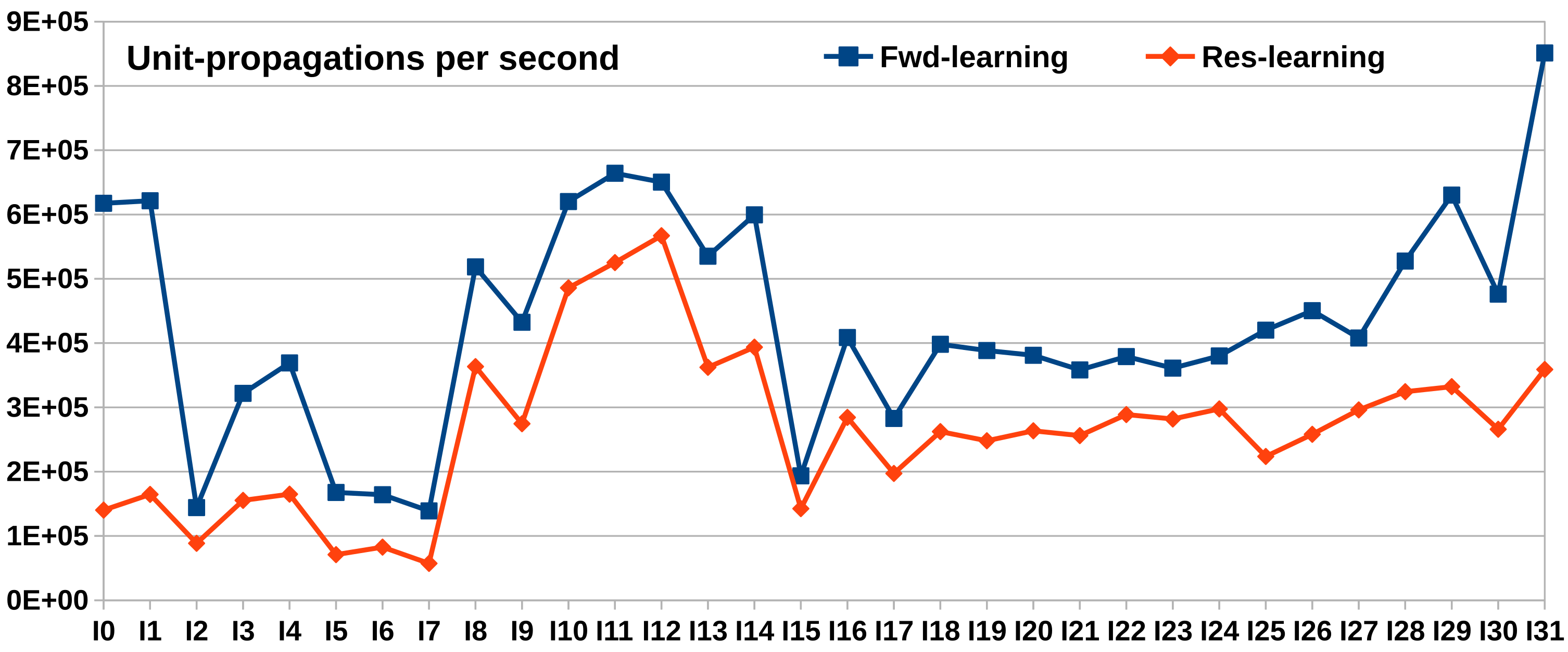
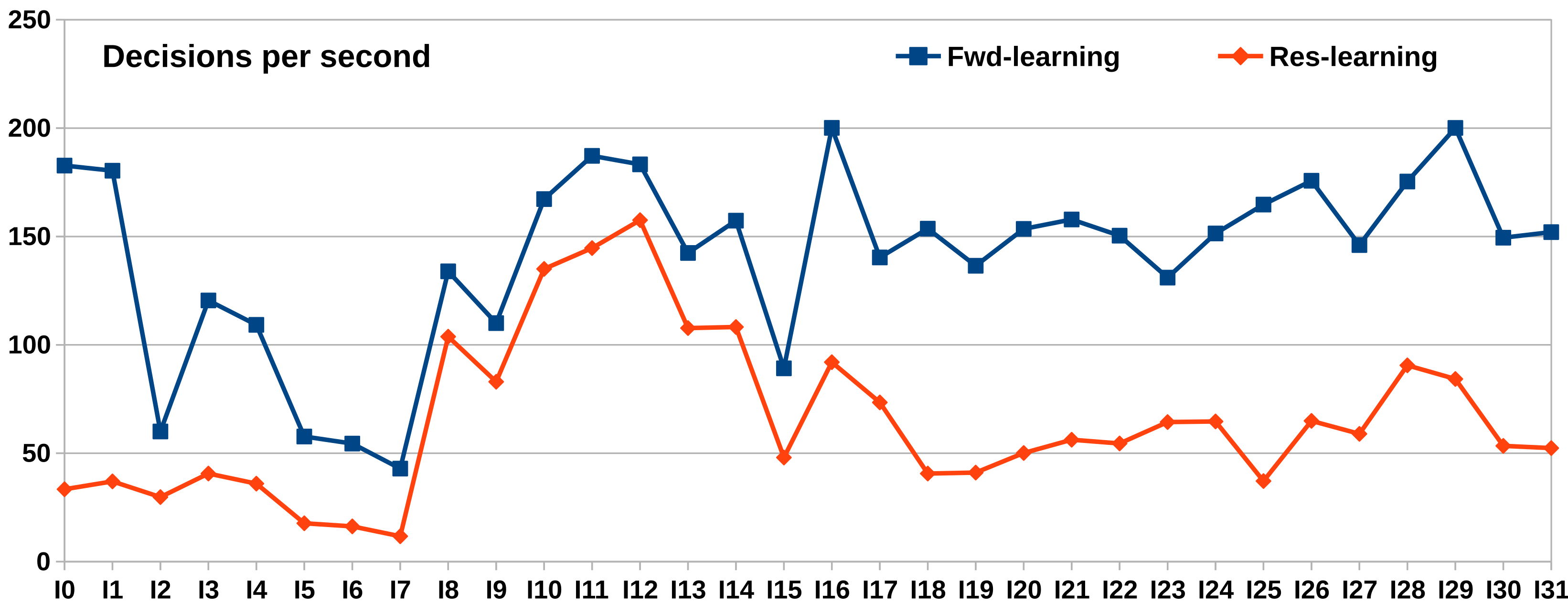
Figure 1: Performance of the two versions of yasmin (using Res-learning and Fwd-learning). Number of propagations per second (top) and number of decisions per second (bottom).

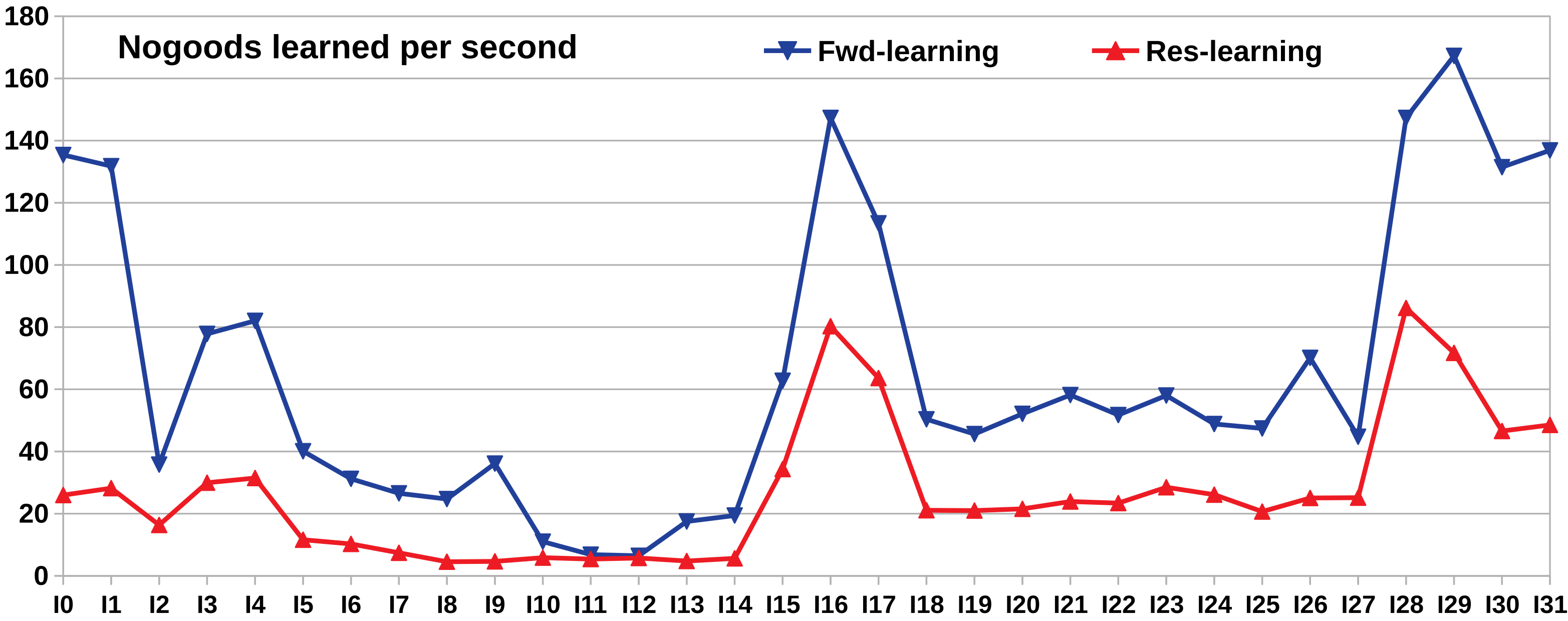
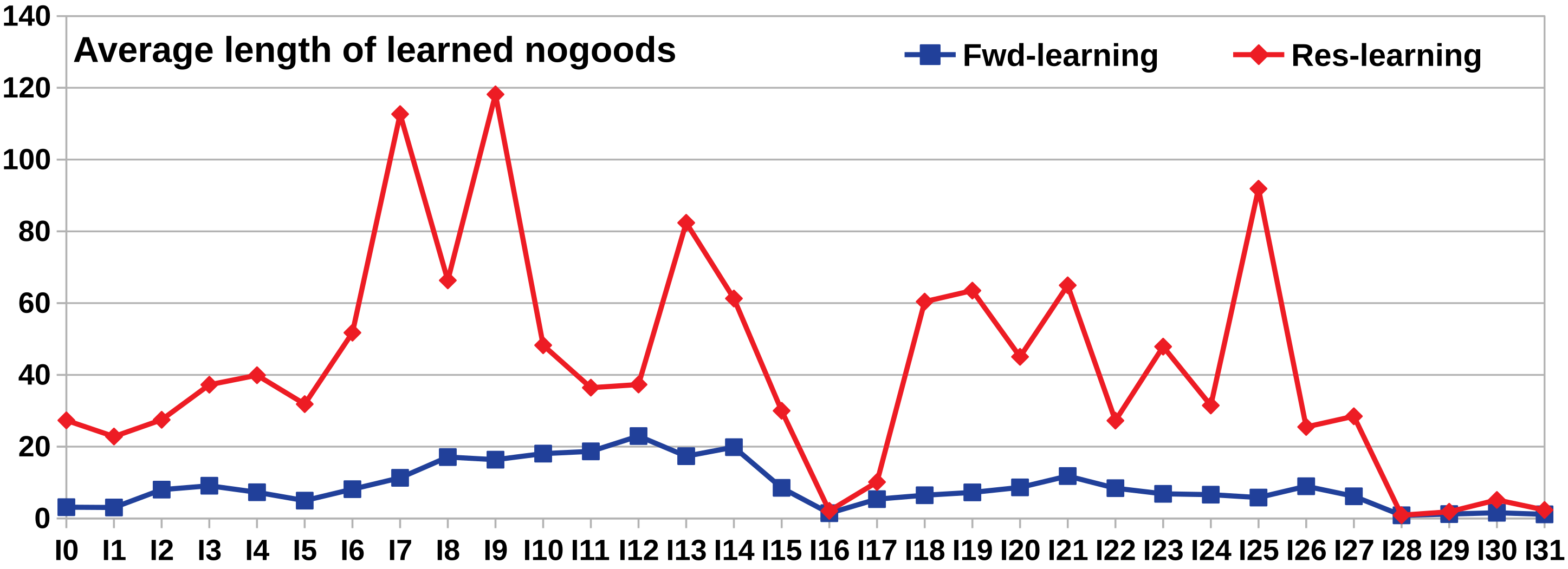
Figure 2: Learned nogoods using Res-learning and Fwd-learning. Number of learned nogoods per second (top) and their average length (bottom).

5 Experimental Results

In this section we briefly report on some experiments we run to compare the two learning techniques described in the previous section. Table 1 shows a selection of the instances (taken from [6]) we used. For each instance the table indicates, together with an ID, the number of nogoods and the number of atoms.

Experiments were run on a Linux PC (running Ubuntu Linux v.19.04), used as host machine, and using as device a Tesla K40c Nvidia GPU with these characteristics: 2880 CUDA cores at 0.75 GHz, 12GB of global device memory. We used on such GPU the CUDA runtime version 10.1. The compute capability was 3.5.

Fig. 1 compares the two versions of yasmin solver, differing only on the used learning procedure. Comparison is made w.r.t. the number of propagations per second and the number of decisions per second performed by the solver. The new learning strategy outperforms the resolution-based one on all instances. The plots in Fig. 2 compare the performance of the two learning procedure in terms of their outcomes. Also from this perspective fwd_learning() exhibits better behavior, producing smaller nogoods in shorter time. Notice that results of the same kind have been obtained with different selection heuristics and varying the parameters of kernel configuration (e.g., number of threads-per-block, grid and block dimensions, etc.). Moreover, results of experiment run on different GPUs are in line with those reported.

Conclusions

This paper we described the main traits of a CUDA-based solver for Answer Set Programming. The fact that the algorithms involved in ASP-solving present an irregular and low-arithmetic intensity, usually combined with data-dependent control flows, makes it difficult to achieve high performance without adopting proper sophisticated solutions and fulfilling suitable programming directives. In this paper we dealt with the basic software architecture of a parallel prototypical solver with the main aim of demonstrating that GPU-computing can be exploited in ASP solving. Much is left to do in order to obtain a full-blown parallel solver able to compete with the state-of-the-art existing solvers. First, effort have to be made in enhancing the parallel solver with the collection of heuristics proficiently used to guide the search in sequential solvers. Indeed, experimental comparison [6] show that good heuristics might be the most effective component of a solver. Second, the applicability of further techniques and refinements have to be investigated. For instance, techniques such as parallel lookahead [4], multiple learning [10], should be considered. Also the possibility of developing a distributed parallel solver that operates on multiple GPUs represents a challenging theme of research.

References

- [1] M. Bernaschi, M. Bisson, E. Mastrostefano, and F. Vella. Multilevel parallelism for the exploration of large-scale graphs. IEEE Trans. on Multi-Scale Comp. Sys., 4(3):204–216, 2018.
- [2] A. Biere, M. Heule, H. van Maaren, and T. Walsh. Handbook of Satisfiability, volume 185 of Frontiers in Artificial Intelligence and Applications. IOS Press, 2009.
- [3] A. Dal Palù, A. Dovier, A. Formisano, and E. Pontelli. CUD@SAT: SAT Solving on GPUs. J. of Experimental & Theoretical Artificial Intelligence (JETAI), 27(3):293–316, 2015.
- [4] A. Dovier, A. Formisano, and E. Pontelli. Parallel answer set programming. In Y. Hamadi and L. Sais, editors, Handbook of Parallel Constraint Reasoning, chapter 7. Springer, 2018.
- [5] A. Dovier, A. Formisano, E. Pontelli, and F. Vella. Parallel Execution of the ASP Computation. In M. De Vos, T. Eiter, Y. Lierler, and F. Toni, editors, Tech.Comm. of ICLP 2015, volume 1433. CEUR-WS.org, 2015.
- [6] A. Dovier, A. Formisano, E. Pontelli, and F. Vella. A GPU implementation of the ASP computation. In M. Gavanelli and J. H. Reppy, editors, PADL 2016, volume 9585 of LNCS, pages 30–47. Springer, 2016.
- [7] E. Erdem, M. Gelfond, and N. Leone. Applications of answer set programming. AI Magazine, 37(3):53–68, 2016.
- [8] A. Falkner, G. Friedrich, K. Schekotihin, R. Taupe, and E. C. Teppan. Industrial applications of answer set programming. Künstliche Intelligenz, 32(2):165–176, 2018.
- [9] A. Formisano, R. Gentilini, and F. Vella. Accelerating energy games solvers on modern architectures. In Proc. of the 7th Workshop on Irregular Applications: Architectures and Algorithms, IA3@SC, pages 12:1–12:4. ACM, 2017.
- [10] A. Formisano and F. Vella. On multiple learning schemata in conflict driven solvers. In S. Bistarelli and A. Formisano, editors, Proc. of ICTCS., volume 1231. CEUR-WS.org, 2014.
- [11] M. Gebser, R. Kaminski, B. Kaufmann, and T. Schaub. Answer Set Solving in Practice. Morgan & Claypool Publishers, 2012.
- [12] M. Gelfond. Answer sets. In F. van Harmelen, V. Lifschitz, and B. W. Porter, editors, Handbook of Knowledge Representation, chapter 7. Elsevier, 2008.
- [13] S. Hong, T. Oguntebi, and K. Olukotun. Efficient parallel graph exploration on multi-core CPU and GPU. In Int. Conf. on Parallel Architectures and Compilation Techniques, pages 78–88. IEEE, 2011.
- [14] F. Lin and J. Zhao. On tight logic programs and yet another translation from normal logic programs to propositional logic. In G. Gottlob and T. Walsh, editors, Proc. of IJCAI-03, pages 853–858. Morgan Kaufmann, 2003.
- [15] L. Liu, E. Pontelli, T. C. Son, and M. Truszczynski. Logic programs with abstract constraint atoms: The role of computations. Artificial Intelligence, 174(3-4):295–315, 2010.
- [16] A. Lumsdaine, D. Gregor, B. Hendrickson, and J. Berry. Challenges in parallel graph processing. Parallel Processing Letters, 17(01):5–20, 2007.
- [17] NVIDIA. CUDA C: Programming Guide (v.10.1). NVIDIA Press, Santa Clara, CA, 2019.
- [18] NVIDIA Corporation. NVIDIA CUDA Zone. https://developer.nvidia.com/cuda-zone, 2019.