Minimax Isometry Method: A compressive sensing approach for Matsubara summation in many-body perturbation theory

Abstract

We present a compressive sensing approach for the long standing problem of Matsubara summation in many-body perturbation theory. By constructing low-dimensional, almost isometric subspaces of the Hilbert space we obtain optimum imaginary time and frequency grids that allow for extreme data compression of fermionic and bosonic functions in a broad temperature regime. The method is applied to the random phase and self-consistent $GW$ approximation of the grand potential. Integration and transformation errors are investigated for Si and SrVO₃.

I Introduction

Calculations of finite temperature properties of materials are becoming progressively important. In particular for metals, a proper treatment of the partial occupancies of orbitals at the Fermi level is absolutely required. For instance, because of a finite Brillouin zone sampling, orbitals at the Fermi level often exhibit degeneracies and partial occupancies that cannot be lifted without resorting to technical tricks (such as shifting the Fermi energy). In mean field calculations, particularly, in density functional theory, finite temperature effects are nowadays usually incorporated using Mermin’s formalism,Mermin (1965); Fu and Ho (1983); De Vita and Gillan (1991); Methfessel and Paxton (1989) which has found wide spread acceptance in most density functional theory codesKresse and Furthmüller (1996) and leads to a concise treatment of the grand potential, the internal electronic energy as well as the entropy related to the electronic degrees of freedom. Partial occupancies of degenerate states at the Fermi level are thereby naturally accounted for.

For correlated wave function and Green’s function based methods, including finite temperature effects and handling partial occupancies of states at the Fermi level is certainly less trivial but absolutely necessary.Kohn and Luttinger (1960); Luttinger and Ward (1960) In Green’s function theory, the common solution is to either treat the Green’s function in imaginary time and describe it in the interval $[-\beta,\beta]$ or to impose periodicity in imaginary time and Fourier transform all relevant quantities to imaginary frequency. This yields the well known Matsubara technique,Matsubara (1955) details of which are explained in many textbooks.Fetter and Walecka (2003); Negele and Orland (1988)

Although working in imaginary frequency and adopting the Matsubara frequencies fundamentally allows to derive simple and compact equations for the grand potential, internal electronic energy or the electronic entropy, calculations using the Matsubara formulation are in many cases unpractical. This is especially so, if the method is combined with first principles plane wave codes or codes using a linear combination of atomic orbitals. For example, let us assume we want to calculate the properties of a material at $T=100$ K. This corresponds to a Matsubara frequency spacing of about $\Delta\omega=2\pi/\beta=50$ meV. In plane wave calculations, the maximum excitation energies are often approaching 200 to 400 eV. To perform the required frequency summations, hence, 4000 to 8000 frequency points are required for meV precision. Clearly, if one were forced to use Matsubara grids, the calculations would become intractable for all but the simplest systems and smallest basis sets. Thus, one has to find a way to “compress” the number of grid points to an affordable small value in order to reduce the compute cost. This is one of the main topics of the present work. Specifically, the goal is to derive in a mathematical concise way optimal non-uniform frequency grids that can be used instead of the standard Matsubara grid. It goes without saying that such grids will always introduce small numerical errors, however, as we demonstrate in this paper, by increasing the number of frequency points, the error drops exponentially. It also needs to be mentioned that these optimal grids will be different for bosonic and fermionic functions. This is similar to the Matsubara technique, which results in grid points $\omega_{m}=(2m+1)\pi/\beta$ for fermions and $\nu_{m}=2m\pi/\beta$ for bosons. In fact, we will see below that this behavior is also roughly maintained for the first few frequency points for our compressed grids.

Another important issue is that Green’s function methods can be made particularly efficient by relying on a dual representation of all quantities in imaginary time and imaginary frequency.Rojas et al. (1995); Rieger et al. (1999); Kaltak et al. (2014a) For instance, the well known Dyson equation $G(\omega)=G_{0}(\omega)+G_{0}(\omega)\Sigma(\omega)G(\omega)$ is most easily solved in the frequency domain, since the equation involves a single frequency point only. On the other hand, the polarizability is most easily calculated in time $t$ or imaginary time $\tau$, e.g. $\chi(t)=-iG(t)G(-t)$ . Thus, for an efficient implementation it is often expedient to be able to switch via Fourier transformations from the imaginary time to the imaginary frequency representation and vice versa without loss of precision. Being capable to switch from imaginary frequency to imaginary time also resolves another issue: as explained above, our compressed grids comprise different frequencies for fermions and bosons. Hence, it is not a simple matter to calculate a bosonic quantity from a fermionic one in frequency space without resorting to interpolation (they are represented on different grids). The imaginary time grid provides the necessary glue between these two grids. The methods that we describe below adopt one and only one common grid in the time domain (which requires a slight compromise in numerical precision). We also derive Fourier coefficients to bring any bosonic or fermionic function to that common time grid. Calculations of bosonic quantities from fermionic ones are than performed in imaginary time $\tau$, for instance $\chi(i\tau)=-G(-i\tau)G(+i\tau)$.

The present work is a natural extension of our own previous work on optimal zero temperature imaginary time and frequency grids.Kaltak et al. (2014b, a) Furthermore, some of the ideas that we pursue here have been touched upon and are inspired by related work published before. To name a few examples: Faleev and coworkers used Keldysh time-loop contours to avoid explicit construction of frequency grids.Faleev et al. (2006) Ku, Wei and Eguiluz suggested non-uniform power grids to reduce the number of grid points.Ku and Eguiluz (2002) Welden and coworkers used a Legendre representation of the imaginary time Green’s function and spline interpolation in the Matsubara domain,Welden et al. (2016) an approach used by several other authors before.Boehnke et al. (2011); Huang (2016) All these techniques have in common that the grids are not tailored for their purpose. Most relevant to our case is the work of Ozaki who approximated the Fermi function by a continued fraction representation of the hypergeometric function.Ozaki (2007) Hu applied the same method to bosons and the Bose-Einstein occupation function.Hu et al. (2010) Shinaoka et. al developed an efficient approach for imaginary time Green’s functions using an intermediate representation between the imaginary time and real frequency domainShinaoka et al. (2017) and Li and coworkers applied Shinaoka’s method to the $GW$ approximation recently.Li et al. (2020)

The general idea of us is to map the optimization of the time and frequency grid, or Fourier coefficients onto a well defined minimization problem. This minimization problem is then solved using Remez’s Minimax algorithm.Remez (1962); Takatsuka et al. (2008) To obtain optimized time and frequency grids we pursue two different routes in the present work, corresponding to different object functions.

The first one is designed for non-selfconsistent perturbational many body calculations, where a non-interacting Greens function is determined from an initial mean field Hamiltonian. As an example, we show results for calculating the correlation energy in the random phase approximation at finite temperature. However, this approach is also applicable to Møller-Plesset perturbation theory or, potentially, coupled cluster methods. The unifying property is that the building blocks are always non-interacting fermionic propagators, which can be readily obtained as resolvent of a one-particle Hamiltonian at any frequency or time point. In this case, it suffices to solve a minimization problem that minimizes the error in second order perturbation theory, akin to the zero temperature case.Häser and Almlöf (1992); Kaltak et al. (2014b)

Somewhat more challenging is the development of efficient sampling schemes for self-consistent Green’s function methods. In this case, the Green’s function is obtained from the Dyson equation at a set of frequency and/or time points. This problem is more challenging, since the frequency and time grids need to be capable to accurately represent all properties of the Green’s function and polarization propagators without loss of the norm or spectral density. Here, we rely on ideas previously presented by Ozaki to design optimal fermionic Matsubara grids that allow to represent the Fermi function with minimal error.Ozaki (2007) We, however, go beyond the work of Ozaki by mapping this problem onto a well define minimization problem.

II Mathematical Formalism

II.1 Matsubara Technique

The Matsubara technique is a way to formulate quantum field theory (QFT) at finite temperature. More precisely, it makes use of the Wick rotation,Wick (1954) which transforms the real time axis of Minkowski spacetime to the imaginary time axis $t\to-i\tau$. Because real space remains unchanged by this transformation, spacetime becomes essentially euclidean, so that this approach is also known as euclidean quantum field theory.Osterwalder and Schrader (1973, 1975)

As Matsubara has shown, the imaginary time integrals in finite temperature perturbation theory are restricted to the interval $-\beta<\tau<\beta$.Matsubara (1955) This has the advantage that one can expand the imaginary time-dependence of the corresponding integrands into a Fourier series, such that imaginary-time integration becomes essentially an (infinite) series over discrete Fourier coefficients. The corresponding discrete frequencies are known as Matsubara frequencies and it is important for us to distinguish between fermionic, denoted by $\omega_{n}$ in the following, and bosonic Matsubara frequencies, denoted by $\nu_{m}$ in the remainder of this paper.

Fermionic Matsubara frequencies represent the non-zero Fourier modes of fermionic functions, while bosonic frequencies are the non-zero modes of bosonic functions. This is explained in more detail below by means of the free-electron Green’s function (Feynman propagator) and the irreducible polarizability, the building blocks of many-body perturbation theory. Furthermore, if the distinction between fermionic and bosonic functions is irrelevant we use the term correlation function.

The free propagator, or non-interacting Green’s function, in imaginary time $\tau$ represents a prototype of a fermionic function. In a one-electron basis, the free propagator is diagonal $g_{\alpha\gamma}(-i\tau)=\delta_{\alpha\gamma}g(x_{\alpha},-i\tau)$ and the entries readNegele and Orland (1988); Fetter and Walecka (2003)

$$g(x_{\alpha},-i\tau)=e^{-x_{\alpha}\tau}\left[(1-f(x_{\alpha}))\Theta(\tau)-f(x_{\alpha})\Theta(-\tau)\right],$$ (1)

where $x_{\alpha}=\epsilon_{\alpha}-\mu$, and $\epsilon_{\alpha}$, $\mu$ and $f$ are the one electron energy, the chemical potential and the Fermi function, respectively. Here $\Theta$ is the Heaviside step function.Olver et al. It is the reason why $g(x_{\alpha},-i\tau)$ changes sign at $\tau=0$. Also, the presence of the step functions implies

$$g(x_{\alpha},-i\beta+i\tau)=-g(x_{\alpha},+i\tau),\quad 0<\tau<\beta.$$ (2)

This anti-symmetric property has an important effect on the Fourier series representation in the interval $-\beta<\tau<\beta$

$$g(x_{\alpha},-i\tau) =\frac{1}{\beta}\sum\limits_{m=-\infty}^{\infty}\tilde{g}(x_{\alpha},i\omega_{m})e^{-i\omega_{m}\tau}$$ (3)

$$\tilde{g}(x_{\alpha},i\omega_{m}) =\int_{-\frac{\beta}{2}}^{\frac{\beta}{2}}\mathrm{d}\tau g(x_{\alpha},-i\tau)e^{i\omega_{m}\tau},$$ (4)

because it contains only fermionic frequencies

$$\omega_{m}=\frac{2m+1}{\beta}\pi,\quad m\in\mathds{Z}.$$ (5)

Here and in the following, $\mathds{Z}$ denotes the set of all integers. The same representation is valid for all fermionic functions on the imaginary time axis, including the self-energy.

An example for a bosonic function is the independent particle polarizability, which is diagonal $\chi_{\alpha\gamma\alpha^{\prime}\gamma^{\prime}}=\delta_{\alpha\alpha^{\prime}}\delta_{\gamma\gamma^{\prime}}\chi_{\alpha\gamma}$ and has the entries

$$\chi_{\alpha\gamma}(-i\tau)=-g(x_{\alpha},-i\tau)g(x_{\gamma},+i\tau).$$ (6)

In contrast to Equ. (2), bosonic functions do not change sign in imaginary time, but are symmetric

$$\chi_{\alpha\gamma}(-i\beta+i\tau)=\chi_{\alpha\gamma}(+i\tau),\quad 0<\tau<\beta.$$ (7)

Consequently, the Fourier expansion

$$\chi_{\alpha\gamma}(-i\tau) =\frac{1}{\beta}\sum\limits_{n=-\infty}^{\infty}\tilde{\chi}_{\alpha\gamma}(i\nu_{n})e^{-i\nu_{n}\tau}$$ (8)

$$\tilde{\chi}_{\alpha\gamma}(i\nu_{n}) =\int_{-\frac{\beta}{2}}^{\frac{\beta}{2}}\mathrm{d}\tau\chi_{\alpha\gamma}(-i\tau)e^{i\nu_{n}\tau}$$ (9)

contains only bosonic frequencies

$$\nu_{n}=\frac{2n}{\beta}\pi,\quad n\in\mathds{Z}.$$ (10)

It is often argued that bosonic (fermionic) functions are periodic (anti-periodic) in $\tau$. This is strictly speaking not correct. The free propagator, for instance, is defined a priori only in the fundamental imaginary time interval $|\tau|\leq\beta$, because (1) grows or decays exponentially for arguments outside (thin lines in Fig. 1). The same holds true for the irreducible polarizability. In fact, only the Fourier expansions (8) and (3) define periodic and anti-periodic functions in $\tau$ with (anti-) period $\beta$. This behavior is illustrated in Fig. 1 showing a typical fermionic and bosonic function. In practice, it is important to recall that exponentially growing terms in propagators are not present, since the $\tau$-integrations are performed over $0<\tau<\beta$ or, equivalently, over $-\beta/2<\tau<\beta/2$. Due to consistency with our previous papersKaltak et al. (2014b, a); Liu et al. (2016) we usually work in the interval $[-\beta/2,\beta/2]$.

Figure 1: (left) Fermionic function $g_{1}+g_{2}$ with $\epsilon_{1}=0.19,\epsilon_{2}=9.12$ eV and $\beta=1$ eV^-1 in the fundamental interval (green line) and its corresponding Fourier series truncated after $m>10$ (blue line). (right) Corresponding bosonic function. Analytic fermionic and bosonic functions either increase or decrease exponentially for $|\tau|>\beta$ (e.g. Equ. (1)), while the corresponding Fourier expansion outside $[-\beta,\beta]$ is (anti-) periodic.

As already explained in the introduction, the Matsubara summation has one major drawback; the series converge very slowly with the number of frequency points, necessitating thousands of grid points (see also Sec. IV.1). However, the Matsubara formalism is an elegant method to derive a closed form for the grand canonical potential $\Omega$ of interacting electrons.Luttinger and Ward (1960); Negele and Orland (1988) The most important contributions to $\Omega$ are summarized in the following section for some commonly used approximations.

II.2 The correlation energy

The RPA can be understood as an infinite sum of all possible ring diagrams. The method becomes exact for the correlation energy of the interacting homogeneous electron gas at very high density as $T\to 0$.Gell-Mann and Brueckner (1957); Bohm and Pines (1951); Pines and Bohm (1952); Bohm and Pines (1953) A closed form of the grand potential in the RPA can be found in Negele and Orland’s bookNegele and Orland (1988) and reads

$$\Omega_{c}^{\rm RPA}=\frac{1}{2}\frac{1}{\beta}\sum\limits_{n\in\mathds{Z}}\mathrm{Tr}\left\{\ln\left[\mathds{1}-\tilde{\chi}(i\nu_{n})V\right]-\tilde{\chi}(i\nu_{m})V\right\},$$ (11)

where $V$ stands for the Coulomb matrix elements and the trace $\mathrm{Tr}$ refers to summation over elements of the basis. In second order this corresponds to the direct term in Møller-Plessett (MP2) perturbation theory:

$$\begin{split}\Omega_{c}^{\rm d-MP2}=&\frac{1}{4}\frac{1}{\beta}\sum\limits_{n\in\mathds{Z}}\mathrm{Tr}\left[\tilde{\chi}(i\nu_{n})V\tilde{\chi}(i\nu_{n})V\right]\\ =&\frac{1}{4}\int_{-\frac{\beta}{2}}^{\frac{\beta}{2}}\mathrm{d}\tau\mathrm{Tr}\left[\chi(-i\tau)V\chi(i\tau)V\right].\end{split}$$ (12)

A key point is that the correlation energy in both, the RPA and MP2, depends only on the polarizability, respectively, on products of two Green’s functions $G(i\tau)G(-i\tau)$. In this sense, the RPA is an approximative bosonization of the original problem, a property that greatly simplifies the construction of appropriate time and frequency grids. Specifically, only the bosonic frequencies $\nu_{n}$ enter in the final evaluation of the correlation energy.

As an example of methods where bosonization is typically not applicable, we decided to evaluate the Galitskii-Migdal (GM) expressionGalitskii and Migdal (1958); Caruso et al. (2013) for the correlation part of the grand potential

$$\begin{split}\Omega_{c}^{\rm GM}=&\frac{1}{\beta}\sum\limits_{m\in\mathds{Z}}\mathrm{Tr}\left[\tilde{G}(i\omega_{m})\tilde{\Sigma}(i\omega_{m})\right]\\ =&\int_{-\frac{\beta}{2}}^{\frac{\beta}{2}}\mathrm{d}\tau\mathrm{Tr}\left[G(i\tau)\Sigma(-i\tau)\right].\end{split}$$ (13)

Here $\tilde{G}$ is the dressed propagator and the solution of the Dyson equation

$$\tilde{G}(i\omega_{m})=\tilde{G}_{0}(i\omega_{m})+\tilde{G}_{0}(i\omega_{m})\tilde{\Sigma}(i\omega_{m})\tilde{G}(i\omega_{m}),$$ (14)

where $\tilde{G}_{0}$ is the Hartree-Fock Green’s function, $\tilde{\Sigma}$ the $GW$ correlation self-energyHedin (1965)

$$\tilde{\Sigma}(i\omega_{m})=\int_{-\beta/2}^{\beta/2}\mathrm{d}\tau G(-i\tau)W(-i\tau)e^{i\omega_{m}\tau}$$ (15)

and $\tilde{W}$ the RPA screened potential

$$\tilde{W}(i\nu_{n})=V+V\tilde{\chi}(i\nu_{n})\tilde{W}(i\nu_{m}).$$ (16)

Considering the equations above, it should be quite obvious why it is substantially more difficult to obtain suitable time and frequency grids in this case. Equ. (16) should be solved on the bosonic frequency grid, whereas all the other quantities need to be evaluated on fermionic grids. This implies that at least two frequency grids (and potentially time grids) are required.

II.3 Odd and even functions of time

We found it expedient to distinguish between the time-symmetric and anti-symmetric part of the Green’s function

$$\hat{u}_{\tau}(x_{\alpha})= \frac{g(x_{\alpha},-i\tau)+g(x_{\alpha},+i\tau)}{2}$$ (17)

$$\hat{v}_{\tau}(x_{\alpha})= \frac{g(x_{\alpha},-i\tau)-g(x_{\alpha},+i\tau)}{2}.$$ (18)

It is easy to show that for the independent particle Green’s function (1) in the interval $[-\beta,\beta]$ the corresponding even and odd functions read

$$\hat{u}_{\tau}(x_{\alpha})= \frac{1}{2}\frac{\sinh\left[\frac{\beta x_{\alpha}}{2}\left(1-2\frac{\left|\tau\right|}{\beta}\right)\right]}{\cosh\left(\frac{\beta x_{\alpha}}{2}\right)}$$ (19)

$$\hat{v}_{\tau}(x_{\alpha})= \frac{\mathrm{sgn}(\tau)}{2}\frac{\cosh\left[\frac{\beta x_{\alpha}}{2}\left(1-2\frac{\left|\tau\right|}{\beta}\right)\right]}{\cosh\left(\frac{\beta x_{\alpha}}{2}\right)}$$ (20)

and have the following Fourier coefficient functions at fermionic Matsubara frequencies $\omega_{n}$

$$\tilde{u}_{\omega_{n}}(x_{\alpha})= \frac{1}{2}\frac{x_{\alpha}}{x_{\alpha}^{2}+\omega_{n}^{2}}$$ (21)

$$\tilde{v}_{\omega_{n}}(x_{\alpha})= \frac{1}{2}\frac{\omega_{n}}{x_{\alpha}^{2}+\omega_{n}^{2}}.$$ (22)

If we generalize the above functions to bosonic functions by defining

$$u_{\tau}(x_{\alpha})= \frac{1}{2}\frac{\cosh\left[\frac{\beta x_{\alpha}}{2}\left(1-2\frac{\left|\tau\right|}{\beta}\right)\right]}{\cosh\left(\frac{\beta x_{\alpha}}{2}\right)}$$ (23)

$$v_{\tau}(x_{\alpha})= \frac{\mathrm{sgn}(\tau)}{2}\frac{\sinh\left[\frac{\beta x_{\alpha}}{2}\left(1-2\frac{\left|\tau\right|}{\beta}\right)\right]}{\cosh\left(\frac{\beta x_{\alpha}}{2}\right),}$$ (24)

we obtain the corresponding bosonic Fourier coefficient functions at bosonic frequencies $\nu_{n}$ as

$$\overline{u}_{\nu_{n}}(x_{\alpha})= \frac{1}{2}\frac{x_{\alpha}}{x_{\alpha}^{2}+\nu_{n}^{2}}\tanh\frac{x_{\alpha}\beta}{2}$$ (25)

$$\overline{v}_{\nu_{n}}(x_{\alpha})= \frac{1}{2}\frac{\nu_{n}}{x_{\alpha}^{2}+\nu_{n}^{2}}\tanh\frac{x_{\alpha}\beta}{2}.$$ (26)

Table 1 summarizes the functions defined in this manner. Note that the bosonic and fermionic function are identical in time, if we restrict the value of $\tau$ to $[0,\beta/2]$. An advantage of defining odd and even functions is that one can restrict all time integrations to the interval $[0,\beta/2]$ and obtain the results from negative imaginary times by symmetry considerations. Also, summations over Matsubara frequencies can be constrained to positive frequencies, since the contributions from negative frequencies follow again from symmetry considerations.

The basis functions defined above reduce to our previously used basis functions in the $\beta\to\infty$ limit.Kaltak et al. (2014b); Liu et al. (2016) More precisely, the even and odd imaginary time basis functions (19), (20), (23), (24) approach all the same limit on the positive $\tau$-axis for $\beta\to\infty$, namely the zero temperature basis function $\frac{1}{2}e^{-|x_{\alpha}\tau|}$. The Fourier bases (25), (26) and (21), (22) separate into two distinct basis functions in this limit (see IC in Tab. 1). This means that for $\beta\to\infty$ there is only one optimal $\tau$-grid and two distinct optimal frequency grids for the functions defined above; a fact that has been exploited by the authors in previous papers.Kaltak et al. (2014a); Liu et al. (2016); Grumet et al. (2018)

The duality principle between time and frequency, which was formulated in our previous papers, allows transformations between grid representations of the same quantity without significant loss in precision. In the present work, it is understood rigorously in terms of almost isometric spaces discussed in the next section. We employ this method to derive a compressed representation of the independent-particle polarizability at finite temperature that allows for accurate summations over bosonic Matsubara frequencies in Section III.

To this end, we prove a general theorem about almost isometric Hilbert spaces that can be used to determine compressed representations for the polarizability in imaginary time and imaginary frequency. The corresponding time and frequency grids are ideal to calculate the RPA correlation energy at finite temperature with a small number of grid points.

Table 1: Almost isometric basis functions $\left\langle\omega\middle|x\right\rangle$ and $\left\langle\tau\middle|x\right\rangle$ related by cosine (subscript 1) or sine transformations (subscript 2) for $\beta=1$. IA₁ and IB₂ represent bosonic (b) functions, whereas IA₂ and IB₁ represent fermionic (f) functions. $\left\langle\omega\middle|x\right\rangle$ must be evaluated at the respective Matsubara grids. Third column shows the corresponding conserved $L^{2}$-norm for $N\to\infty$ (given by Equ. (29)). From the infinite set of basis functions a discrete set with time points $\{\tau_{j}^{*}\}_{j=1}^{N}$ and frequency points $\{\omega_{k}^{*}\}_{k=1}^{N}$ will be selected to independently minimize the errors in the $L^{2}$-norm tabulated in the column $\|x\|_{2}^{2}$. IB₂ is not relevant for the present work, since polarization propagators observe the symmetries IA₁.

group		$\left\langle\tau\middle|x\right\rangle$	$\left\langle\omega\middle|x\right\rangle$	$\|x\|_{2}^{2}$
IA1	b	$\frac{1}{2}\frac{\cosh\frac{x}{2}(1-2|\tau|)}{\cosh\frac{x}{2}}$	$\frac{1}{2}\frac{x\tanh\frac{x}{2}}{x^{2}+\omega^{2}}$	$\frac{\tanh\frac{x}{2}}{4x}+\frac{1-\tanh^{2}\frac{x}{2}}{8}$
IA2	f	$\frac{\mathrm{sgn}(\tau)}{2}\frac{\cosh\frac{x}{2}(1-2|\tau|)}{\cosh\frac{x}{2}}$	$\frac{1}{2}\frac{\omega}{x^{2}+\omega^{2}}$
IB1	f	$\frac{1}{2}\frac{\sinh\frac{x}{2}(1-2|\tau|)}{\cosh\frac{x}{2}}$	$\frac{1}{2}\frac{x}{x^{2}+\omega^{2}}$	$\frac{\tanh\frac{x}{2}}{4x}-\frac{1-\tanh^{2}\frac{x}{2}}{8}$
$[$IB2$]$	b	$\frac{\mathrm{sgn}(\tau)}{2}\frac{\sinh\frac{x}{2}(1-2|\tau|)}{\cosh\frac{x}{2}}$	$\frac{1}{2}\frac{\omega\tanh\frac{x}{2}}{x^{2}+\omega^{2}}$
IC1	b	$\frac{1}{2}e^{-|x\tau|}$	$\frac{1}{2}\frac{|x|}{x^{2}+\omega^{2}}$	$\frac{1}{4x}$
IC2	f	$\frac{\mathrm{sgn}(\tau)}{2}e^{-|x\tau|}$	$\frac{1}{2}\frac{\omega}{x^{2}+\omega^{2}}$

Figure 2: (left) Fermionic basis functions $\left\langle\tau\middle|x\right\rangle$ IA₂ (thick line) and IB₁ (thin line) in imaginary time for $x=10$. (right) Corresponding bosonic basis functions IA₁ (thick) and IB₂ (thin).

For fermionic functions, the situation is more complicated, because the Green’s function $\tilde{G}$ or the self-energy $\tilde{\Sigma}$ can be represented only using both basis functions (21) and (22). How to obtain a compressed fermionic frequency grid that describes both basis functions accurately is discussed in section IV.

III Time and Frequency Grids for RPA

Obviously, for every one-electron energy $x_{\alpha}$, one obtains a corresponding contribution to the Green’s functions $\hat{v}_{\tau}(x_{\alpha}),\hat{u}_{\tau}(x_{\alpha})$ and $\tilde{v}_{\omega}(x_{\alpha}),\tilde{u}_{\omega}(x_{\alpha})$, respectively. Likewise, for a typical transition energy $x_{\alpha}=\epsilon_{\rm unocc}-\epsilon_{\rm occ}$, one obtains contributions to the independent particle polarizability $\chi$ following approximately $v_{\tau}(x_{\alpha}),u_{\tau}(x_{\alpha})$ and $\overline{v}_{\omega}(x_{\alpha}),\overline{u}_{\omega}(x_{\alpha})$ in time and frequency. The relevant question is whether one can chose an optimal discrete set of frequencies $\omega_{k}^{*}$ and time points $\tau_{k}^{*}$ $k=1,...,N$ with corresponding functions that allow to represent all possible contributions to the Green’s function and polarizability accurately. Importantly, in the next subsection we will drop the constraint that the frequencies must correspond to Matsubara frequencies, but we maintain the functional form for the frequency dependence. This is a key step of the present approach.

III.1 Minimax Isometry

To keep the notation simple, we consider the case $\beta=1$ eV^-1 in the following. The general case $\beta\neq 1$ follows from scaling relations that are discussed in III.3 and III.4. The energy levels and transition energies are supposed to be bound $x\in[0,x_{\rm max}]$, as is typically the case in first principles calculations. That is, the interval length $x_{\rm max}$ is either the largest eigenenergy $(\epsilon_{\rm max}-\mu)\beta$ or the largest transition energy $(\epsilon_{\rm max}-\epsilon_{\rm min})\beta$. Furthermore, we consider the functions $v_{\tau}(x),u_{\tau}(x),\tilde{u}_{\omega}(x),\cdots$ as the time and frequency representations of an abstract vector $\left\lvert x\right\rangle$ in a Hilbert space $\mathcal{H}$ and define the in-products $\langle\tau\left\lvert x\right\rangle$ as its imaginary time and $\langle\omega\left\lvert x\right\rangle$ as its imaginary frequency representation, which are equivalent to the corresponding functions in Tab. 1.

It is assumed that $\left\lvert\tau\right\rangle$ and $\left\lvert n\right\rangle$ (shorthand for $\lvert\omega_{n}\rangle$ or $\lvert\nu_{n}\rangle$) are two complete basis sets in imaginary time and frequency for the same function space, such that the identity operator $\mathds{1}$ can be expressed as

$$\mathds{1}= \int_{0}^{1/2}\mathrm{d}\tau\left\lvert\tau\right\rangle\left\langle\tau\right\rvert$$ (27)

$$\mathds{1}= \sum_{n\in\mathds{Z}}\left\lvert n\right\rangle\left\langle n\right\rvert.$$ (28)

From a functional analysis perspective, one says that the two spaces $\mathcal{X}=\mathrm{span}\{\left\lvert\tau\right\rangle\}_{\tau\in[0,1/2]}$ and $\tilde{\mathcal{X}}=\mathrm{span}\{\left\lvert n\right\rangle\}_{n\in\mathds{Z}}$ are isometric with respect to the scalar product induced norm $\|x\|_{2}=\sqrt{\left\langle x\middle|x\right\rangle}$ so that $(\mathcal{X},\left\langle\cdot\middle|\cdot\right\rangle)\cong(\tilde{\mathcal{X}},\left\langle\cdot\middle|\cdot\right\rangle)$. This isometry (indicated by the symbol $\cong$) is effectively a simple basis transformation that does not change the induced norm, since

$$\begin{split}\|x\|_{2}^{2}=\left\langle x\middle|x\right\rangle=&\int_{0}^{1/2}\mathrm{d}\tau\left\langle x\middle|\tau\right\rangle\left\langle\tau\middle|x\right\rangle\\ =&\sum_{n\in\mathds{Z}}\left\langle x\middle|n\right\rangle\left\langle n\middle|x\right\rangle.\end{split}$$ (29)

It is a simple matter, to show that both the time integral as well as the frequency summation in Equ. (29) indeed yield the same result, which are shown in the final column in Tab. 1 (this shows that the two basis sets are indeed isometric).

If $\left\lvert\tau\right\rangle$ is the time and $\left\lvert n\right\rangle$ the discrete frequency basis for fermions (bosons), then $\left\langle\tau\middle|n\right\rangle$ and $\left\langle n\middle|\tau\right\rangle$ are the matrix elements $\cos(\omega_{n}\tau),\sin(\omega_{n}\tau),\cos(\nu_{n}\tau)$ or $\sin(\nu_{n}\tau)$ of the forward and backward basis transformation. Consequently, the two spaces $\mathcal{X}$ and $\tilde{\mathcal{X}}$ are equivalent and span the same Hilbert space $\mathcal{H}$. This equivalence holds true only if infinitely many basis vectors are considered; for finite dimensional subspaces the perfect isometry (29) is violated.

One may illustrate the violation of the isometry (29) with the discrete Fourier transform (DFT) having the bases $\left\lvert\tau_{k}\right\rangle=\left\lvert\frac{1}{2N}(2k-1)\right\rangle$ with $(k=1,\cdots,N)$ and $\left\lvert n\right\rangle=\lvert\pi(2n-1)\rangle$ (truncated fermionic Matsubara grid). The corresponding completeness relations (27), (28) become projectors onto finite dimensional subspaces $X\subset\mathcal{X},\tilde{X}\subset\tilde{\mathcal{X}}$ and have the form

$$P= \frac{1}{2N}\sum\limits_{k=1}^{N}\left\lvert\tau_{k}\right\rangle\left\langle\tau_{k}\right\rvert$$ (30)

$$\tilde{P}= \sum_{n=-N+1}^{N}\left\lvert n\right\rangle\left\langle n\right\rvert=2\sum_{n=1}^{N}\left\lvert n\right\rangle\left\langle n\right\rvert$$ (31)

Only in the limit $N\to\infty$ the projectors approach the identity operator $\mathds{1}$. For finite $N$, the isometry (29) is violated, but can be replaced by a so-called $\varepsilon$-isometryFleming and Jamison (2002); Ding (1988)

$$\|P-\tilde{P}\|:=\max_{0\leq x\leq x_{\rm max}}|\left\langle x\right\rvert P-\tilde{P}\left\lvert x\right\rangle|\leq\varepsilon.$$ (32)

Of interest to us is the magnitude of $\varepsilon$ and especially how it decreases with increasing $N$. For instance, in the case of the DFT $\left\langle x\right\rvert P\left\lvert x\right\rangle$ is the Riemann sum of the integral in (29) of order $N$ and is known to be a poor method to evaluate integrals. As a consequence, $\varepsilon$ of the Matsubara grid is a weakly decaying function in $N$ and cannot be used for our purposes, as shown in section V.1.

The following question naturally arises: how can one determine $\varepsilon$-isometric subspaces $X=\mathrm{span}\{\left\lvert\tau_{k}\right\rangle\}_{k=1}^{N}$, and $\tilde{X}=\mathrm{span}\{\left\lvert\omega_{k}\right\rangle\}_{k=1}^{N}$, such that the completeness relations (27) and (28) are approximated as good as possible for all vectors $\left\lvert x\right\rangle$ with $0\leq x\leq x_{\rm max}$?

Using the notation in (32), the answer to this question are the solutions of following minimax problems:

$$\min_{\sigma_{k}>0,\tau_{k}\in(0,1/2)} \left\|\mathds{1}-\sum\limits_{k=1}^{N}\sigma_{k}\left\lvert\tau_{k}\right\rangle\left\langle\tau_{k}\right\rvert\right\|$$ (33)

$$\min_{\lambda_{k}>0,\omega_{k}>0} \left\|\mathds{1}-\sum\limits_{k=1}^{N}\lambda_{k}\left\lvert\omega_{k}\right\rangle\left\langle\omega_{k}\right\rvert\right\|.$$ (34)

Provided the solutions exist, they are known to yield errors $\varepsilon$ that decay exponentially with $N$.Braess (1986) In the following, we prove that (33) and (34) satisfy our requirements.

To prove the assertion above it suffices to show that the minimax errors are an upper bound for the isometry violation in (32). Therefore, assume $\{\sigma_{k}^{*},\tau_{k}^{*}\}_{k=1}^{N}$ and $\{\lambda^{*}_{k},\omega_{k}^{*}\}_{k=1}^{N}$ are the solutions of (33) and (34) with $P^{*}=\sum_{k=1}^{N}\sigma^{*}_{k}\left\lvert\tau_{k}^{*}\right\rangle\left\langle\tau_{k}^{*}\right\rvert$ and $\tilde{P}^{*}=\sum_{k=1}^{N}\lambda^{*}_{k}\left\lvert\omega_{k}^{*}\right\rangle\left\langle\omega_{k}^{*}\right\rvert$ the corresponding projectors, respectively. Then a positive number $\varepsilon/2$ exists (for every given $N$) as an upper bound for (33) and (34) and one can write

$$\begin{split}\Big{\|}\mathds{1}-P^{*}\Big{\|}\leq&\frac{1}{2}\varepsilon\\ \left\|\mathds{1}-\tilde{P}^{*}\right\|=\left\|\tilde{P}^{*}-\mathds{1}\right\|\leq&\frac{1}{2}\varepsilon.\end{split}$$ (35)

Adding both inequalities in (35) and using the triangle inequality $\|f+g\|\leq\|f\|+\|g\|$ (satisfied by every normvon Querenburg (2013)) one obtains

$$\begin{split}\underbrace{\Big{\|}\mathds{1}-P^{*}\Big{\|}+\left\|\tilde{P}^{*}-\mathds{1}\right\|}_{\left\|\mathds{1}-P^{*}+\tilde{P}^{*}-\mathds{1}\right\|\leq}\leq\varepsilon.\end{split}$$ (36)

Last inequality implies (32) for the projectors $P^{*},\tilde{P}^{*}$ and concludes our proof. ∎

This is a quite remarkable result, because it means that the projectors $P^{*}$ and $\tilde{P}^{*}$ converge to the identity operator and, thus, define $\varepsilon$-isometric topological vector spaces $X^{*},\tilde{X}^{*}$ that have the approximation property.Axler et al. (1999) A summary of $\varepsilon$-isometric bases is given in Tab. 1 and discussed below.

Note that the discussion above does not give a prescription how to determine the transformation $X^{*}\to\tilde{X}^{*}$; a corresponding method is presented in section V.1.

The proof above contains only an upper bound for the transformation error in (36). This upper bound $\varepsilon$ is inherited from the sum of the convergence rate of the minimax solutions in the $\tau$- and $\omega$-domain. This convergence rate has been studied by Braess and Hackbusch for the minimax problem IC in the $\tau$-domain listed in Tab. 1. They obtained $\varepsilon(N)\approx 6.7\log(2+N)e^{-\pi\sqrt{2N}}$ for $x\in[1,R_{N}]$, where $[1,R_{N}]$ belongs to the largest possible error for a given order $N$.Braess and Hackbusch (2005) Our numerical experiments discussed in section VII indicate similar convergence rates for all other minimax problems in Tab. 1. In contrast, the DFT or Matsubara grid has only a linear rate of convergence $\varepsilon(N)\propto N^{-1}$.

III.2 Discussion of Isometry

In this subsection, we try to give more insight into what we have achieved at this point. We start with the IC basis, which has been used in previous publications by the authors to construct optimized minimax grids for low scaling random phase and $GW$ algorithms at zero temperature using a different line of arguments.Kaltak et al. (2014b, a); Liu et al. (2016) Specifically, $\left\langle\tau\middle|x\right\rangle$ of IC₁ describes the imaginary time dependence of the independent particle polarizability at zero temperature for a transition energy $x$, while the corresponding $\left\langle\nu\middle|x\right\rangle$ functions describe its imaginary frequency dependence.Kaltak et al. (2014b) The corresponding conserved $L^{2}$-norm (forth column of Tab. 1) is the key quantity for the second order contributions to the correlation energy (see Equ. (12) or Ref. Kaltak et al., 2014b; Takatsuka et al., 2008). These contributions involve energy denominators of the form $1/(2\epsilon_{a}-2\epsilon_{i})$ and are considered to be bound, i.e. virtual states with energies $\epsilon_{a}$ are separated by a band gap $\Delta_{ai}$ from occupied states with energy $\epsilon_{i}$.Kaltak et al. (2014b) The induced norm is important and essentially tells the optimization in the minimax problem which contributions to the energy are most relevant. With this choice, contributions from small energy differences dominate over contributions from large energy differences, hence in the frequency space the grid points will be more densely spaced at small frequencies.

The $\tau$-basis function of IC₂ has the same time dependence (apart from the opposite sign on the negative $\tau$-axis), while the imaginary frequency dependence of the cosine transformation differs considerably from the one obtained from the sine transform (compare $\left\langle\omega\middle|x\right\rangle$ of IC₁ and IC₂). It comes with no surprise that the minimax frequency grids for both are different too.Liu et al. (2016) However, the time grids are identical, and the minimax isometry guarantees that one can map in time between IC₁ and IC₂ with high precision.

Next, we consider the four basis functions of group IA and IB. They can be grouped into bosonic (IA₁ and IB₂) and fermionic (IA₂ and IB₁) pairs. When optimizing the frequency grid points using the minimax algorithm, we allow $\omega$ in IA and IB to deviate from the corresponding Matsubara grid. Indeed, the corresponding Minimax solutions are non-uniformly distributed, but nevertheless closely match Matsubara frequencies at small $\omega$. It turns out, as shown in section VII, that this freedom allows us to describe the high frequency tail of the correlation functions with high precision even in low dimensional subspaces $X^{*},\tilde{X}^{*}$ without the need for interpolation. The corresponding $\varepsilon$-isometric time basis functions have the fermionic anti-symmetry [Equ. (2)] and bosonic symmetry [Equ. (7)] for $-\beta/2\leq\tau\leq\beta/2$, respectively, and are illustrated in Fig. 2.

At finite temperature, the situation is analogous to the zero temperature case, i.e. the conserved $L^{2}$-norm of the IA isometry describes the second order contribution to the correlation part of the grand-canonical potential defined in Equ. (12) (see appendix A). Because of time-inversion symmetry, the polarizability, the screened potential, or contributions to the correlation energy can be entirely presented by IA₁ basis functions since e.g. $\chi(-i\tau)=\chi(-i\beta+i\tau)$ (blue lines in Fig. 2 right). Thus, the isometry IA₁ can be employed to obtain compressed time and frequency grids for the calculation of the correlation part of the grand canonical potential in the RPA as well as MP2. The corresponding imaginary time and frequency grid are discussed in III.3 and III.4, respectively.

As already emphasized before, if we use self-consistent techniques and the GM formula for the grand canonical potential the construction of optimal time and especially frequency grids becomes more difficult, since even and odd basis functions in the frequency domain (IB₁ and IA₂) contribute to the grand potential and have different $L^{2}$-norms (compare third column of IA and IB). We, therefore, propose an alternative approach in this case that is based on the minimization of the $L^{1}$-quadrature error instead (see section IV.1).

III.3 Imaginary time grid

To construct an imaginary time grid for arbitrary $\beta$, we make use of the scaling properties

$$\tau_{j}\to\beta\tau_{j},\quad\sigma_{j}\to\beta\sigma_{j}$$ (37)

that allow to recover the time quadrature for an arbitrary interval $[0,\beta/2]$ from the unscaled solution determined for $[0,1/2]$.

How to chose the bosonic time grid (IA₁) has been discussed in the previous section. However, we also need a time grid to represent fermionic quantities, such as the Green’s functions from which the polarizabilities are build as $g(-i\tau)g(+i\tau)$. For computational reasons, it is obviously desireable to use only one time grid, since this allows us to represent the Green’s functions and the bosonic quantities on the same time grid. The even and odd basis functions of the IA and IB $\varepsilon$-isometry in Tab. 1 are clearly identical for fermions and bosons at positive $\tau$,

$$u_{\tau}(x)= \frac{1}{2}\frac{\cosh\frac{x}{2}(1-2\tau)}{\cosh\frac{x}{2}},\quad\tau>0$$ (38)

$$v_{\tau}(x)= \frac{1}{2}\frac{\sinh\frac{x}{2}(1-2\tau)}{\cosh\frac{x}{2}},\quad\tau>0.$$ (39)

Odd functions are not relevant for bosons as argued above, however, they do matter for fermions, and optimization of the time grid for even and odd functions yields different time grids. We opt to use the optimal even time grid (IA₁) as a common grid for both fermionic and bosonic functions and summarize the relevant arguments here. (i) The second order and RPA correlation energy depends only on bosonic functions, e.g. the polarizability. Hence the fermionic functions are only used at an intermediate stage. (ii) The imaginary time grid for the even functions $u$ yields a small minimax error also for the odd basis functions $v$ for the entire interval $x\in[0,x_{\rm max}]$, with larger but still negligible errors even for $x\to 0$. We suspect that this is due to the fact that in the zero temperature limit $\beta\to\infty$ both basis functions (38) and (39) approach smoothly the same exponential form in the interval $\tau\in[0,1/2]$ (see IC isometry in Tab. 1).

In summary, we solve the minimax problem (33) only for IA₁ $\left\langle\tau_{j}\middle|x\right\rangle=u_{\tau_{j}}(x)=:u_{j}(x)$ and use the same time grid points $\tau_{j}$ for the odd fermionic basis functions. To obtain the minimax time grid points $\tau^{*}_{j}$, it is convenient to rewrite the minimax problem (33) into the following form

$$\min_{\sigma_{j}>0,\tau_{j}\in(0,1/2)}\max_{0\leq x\leq x_{\rm\max}}\left|\|x\|_{2}^{2}-\sum\limits_{j=1}^{N}\sigma_{j}u_{j}^{2}(x)\right|$$ (40)

with $x_{\rm max}=\beta\epsilon_{\max}$ and $\epsilon_{\max}$ the maximum one-electron energy considered. Then it becomes evident that (40) is a non-linear fitting problem of separable type,Golub and Pereyra (2003) which in general has only a solution, if every basis function $u_{j}$ is linearly independent and has less than $N-1$ zeros. The alternant theorem then impliesBraess (1986); Hammerlin and Hoffmann (1994) a set of points $\{x^{*}_{k}\}_{k=0}^{2N}$ (alternant) and a set of non-linear equations

$$\|x_{k}^{*}\|_{2}^{2}-\sum\limits_{j=1}^{N}\sigma^{*}_{j}u^{2}_{\tau_{j}^{*}}(x_{k}^{*})=(-1)^{k}E_{N}$$ (41)

with

$$E_{N}=\pm\max_{0\leq x\leq x_{\rm max}}\left|\|x\|_{2}^{2}-\sum\limits_{j=1}^{N}\sigma_{j}u^{2}_{j}(x)\right|$$ (42)

being positive (negative) if the left hand side of (41) is positive (negative) at $x=x_{0}^{*}$.

The alternant theorem provides the basis for the non-linear Remez algorithm that has been used successfully in other papers and yields the minimax solution $\{\sigma_{j}^{*},\tau_{j}^{*}\}_{j=1}^{N}$.Braess and Hackbusch (2005); Takatsuka et al. (2008); Kaltak et al. (2014b) The minimax solution also yields abscissas in the unscaled interval $0\leq\tau^{*}_{j}\leq\frac{1}{2}$ and the corresponding weights $\sigma^{*}_{j}$ are positive and satisfy the sum rule $\lim_{N\to\infty}\sum_{j=1}^{N}\sigma^{*}_{j}=1$. This is important for the application in many-body theory, since the conservation of particles is guaranteed with increasing $N$ including particles with energy $\epsilon_{\alpha}\approx\mu$.

Before we discuss the construction of the frequency grids a last remark is in place here. The quadrature obtained from the solution of (40) is also a good approximation to the solution for the corresponding problem for the odd basis function (39). On the other hand, the linear combination of $u_{\tau}(x)$ and $v_{\tau}(x)$ yields a similar basis $e^{-\frac{x}{2}(1-2|\tau|)}/\cosh\frac{x}{2}$ that has been used recently by Shinaoka and coworkers to compress Green’s functions on the imaginary time axis in quantum Monte Carlo algorithms.Shinaoka et al. (2017) This, implies a close connection to our method. However, Shinaoka et al. determine the grid as the solution of an integral equation and the connection to $\varepsilon$-isometric subspaces is not immediately evident.

III.4 Bosonic Frequency Grid

To construct the bosonic frequency grid we use the $\varepsilon$-isometric basis of the even time basis (38), specifically again the IA₁ basis

$$\overline{u}_{\nu_{n}}(x)=\frac{x}{x^{2}+\nu_{n}^{2}}\tanh\frac{x}{2}.$$ (43)

The motivation behind this choice is three-fold. Firstly, it is obtained from the cosine transformation of the even time basis (38) and it is suitable for bosonic quantities. Thus it can describe the imaginary frequency dependence of the polarizability (6) that is of bosonic nature; the IA₂ basis is obtained from the sine transform of these functions and has fermionic symmetry and hence irrelevant for the evaluation of bosonic integrals. Secondly, we can use the minimax isometry method to switch between the frequency and time representation of the polarizability with high precision. This follows from the theorem proved in section III.1 Equ. (32). Lastly, the infinite bosonic Matsubara series of the RPA grand potential (11) can be evaluated with high precision without using any interpolation technique.

In practice, the unscaled bosonic frequency quadrature for $\beta=1$ is determined first and following scaling relations are used to obtain the result for arbitrary inverse temperatures

$$\nu_{k}\to\frac{\nu_{k}}{\beta},\quad\lambda_{k}\to\frac{\lambda_{k}}{\beta}.$$ (44)

The corresponding minimax problem reads

$$\min_{\lambda_{k}>0,\nu_{k}\in(0,\infty)}\max_{0\leq x\leq x_{\rm max}}\left|\|x\|_{2}^{2}-\sum\limits_{k=1}^{N}\lambda_{k}\overline{u}^{2}_{\nu_{k}}(x)\right|$$ (45)

where the $L^{2}$-norm $\|x\|_{2}^{2}$ is given in Tab. 1. The solution $\{\lambda_{k}^{*},\nu_{k}^{*}\}_{k=1}^{N}$ is called IA₁-quadrature in the following, in agreement with the notation used in Tab. 1.

IV Frequency Grid for GM

In this section, we discuss the construction of a compressed fermionic frequency grid for selfconsistent Green’s function calculations using Equ. (14), and evaluation of the correlation energy using the GM expression for the grand potential (13).

Ideally, quadratures of the GM expression should be converging exponentially with the number of grid points $N$. In contrast to the polarization function and second order correlation energies, this requires an accurate handling of fermionic functions of the type IA₂ and IB₁ in the frequency domain, which is an intricate problem.

Why the evaluation of the GM energy is more difficult than calculation of the correlation energy for the RPA is discussed in the appendix B in detail. The problem is, however, also obvious, when we desire to calculate the self-consistent Green’s function from the self-energy using the Dyson equation [compare Equ. (14)]. The optimization of the frequency grid yields widely different frequencies for the symmetric and anti-symmetric part of the Green’s function. However clearly, in order to solve the Dyson equation, we need both the symmetric and anti-symmetric part of the Green’s function on the same frequency grid. Attempts to chose one grid over the other yields slow convergence of the total correlation energy. A solution to this dilemma is presented in the following section.

IV.1 Fermionic Frequency Grid via $L^{1}$-norm

Every fermionic Matsubara series of a function $\tilde{A}$ (e.g. $\tilde{A}=\tilde{G}(z)\tilde{\Sigma}(z)$), $\sum_{n\in\mathds{Z}}\tilde{A}(\omega_{n})$, corresponds to a complex contour integral of that function times the Fermi function (see derivation below or Fetter and WaleckaFetter and Walecka (2003)). Hence, finding approximations of the Fermi function with as few poles as possible accelerates the calculation of any Matsubara series by replacing the Matsubara summation by a summation over the poles of the approximated Fermi function.

This idea was exploited by OzakiOzaki (2007) in combination with the following identity for the Fermi function

$$f(x)-\frac{1}{2}=\frac{1}{2}\tanh\frac{x}{2}=\sum\limits_{m\in\mathds{Z}}\underbrace{\frac{x}{x^{2}+\omega_{m}^{2}}}_{\tilde{u}_{\omega_{m}}(x)}.$$ (46)

A proof of this identity is found in the appendix C. Ozaki used a partial fraction decomposition of the hyperbolic tangent in combination with a continued fraction representation of the hypergeometric function ${}_{1}F_{0}$ to derive a compressed form of (46).

Our approach is based on the observation that the $L^{1}$-norm of our previously defined basis functions $\tilde{u}_{\omega_{m}}(x)$

$$\|x\|_{1}=\sum\limits_{m\in\mathds{Z}}|\tilde{u}_{\omega_{m}}(x)|=\frac{1}{2}\tanh\frac{|x|}{2},$$ (47)

is also equivalent to the hyperbolic tangent and thus the Fermi function. This suggests to determine the frequency points and weights by solving the following minimization problem:

$$\min_{\gamma_{k},\omega_{k}>0}\max_{0\leq x\leq x_{\rm max}}\left|\|x\|_{1}-\sum\limits_{k=1}^{N}\gamma_{k}|\tilde{u}_{\omega_{k}}(x)|\right|.$$ (48)

Clearly this is very similar to Equ. (45), but replaces the $L^{2}$- by the $L^{1}$-norm. Because $\|x\|_{2}\leq\|x\|_{1}$ holds true for any $0\leq x\leq x_{\rm max}$,Fleming and Jamison (2002) the $L^{1}$-solution $\{\gamma_{k}^{*},\omega_{k}^{*}\}_{k=1}^{N}$, called F-quadrature in the following, yields linearly independent basis functions $\tilde{u}^{*}_{k}$ that span a larger function space than the basis obtained from corresponding $L^{2}-$solutions discussed in the appendix B. Our numerical experiments presented below show that the F-quadrature evaluates the infinite sum over both, even and odd functions [see Equ. (74)] with high precision for increasing $N$.

Both, the F-quadrature and Ozaki’s hypergeometric quadrature (OHQ), use essentially a rational polynomial approximation to the hyperbolic tangent. In the following, we show why this approach also provides a good approximation of fermionic Matsubara series, such as the the density matrix $\Gamma$ for holes (upper sign) and electrons (lower sign). The density matrix $\Gamma$ satisfies the following identity

$$\Gamma=\pm\lim_{\eta\to 0\pm}G(-i\eta)=\pm\lim_{\eta\to 0\pm}\frac{1}{\beta}\sum\limits_{n=-\infty}^{\infty}\tilde{G}(i\omega_{n})e^{-i\omega_{n}\eta},$$ (49)

where $G$ and $\tilde{G}$ is the interacting Green’s function in imaginary time and on the Matsubara axis, respectively. Specifically, we show that the last expression on the right hand side of (49) can be approximated with the following quadrature formula

$$\Gamma\approx\frac{\mathrm{sgn}(\eta)}{2}\mathds{1}+\sum\limits_{k=1}^{N}\frac{\sigma_{k}}{2}\left[\tilde{G}(i\omega_{k})+\tilde{G}(-i\omega_{k})\right],$$ (50)

where $\mathds{1}$ is the identity matrix in the considered basis and $\sigma_{k},\omega_{k}$ are either the OHQ- or F-quadrature points.

Figure 3: Integration contours in (52) (zigzag line) branch cut of $\tilde{A}$, (crosses) fermionic Matsubara frequencies $\omega_{n}$ correspond to poles $z=i\omega_{n}$ of auxiliary function $h_{\eta}(z)$ defined in (53) and (54) such that contour integral $\oint\mathrm{d}z\tilde{A}(z)h_{\eta}(z)$ for path $\mathcal{C}$ is zero.

To derive Equ. (50) and motivate why an approximation to the hyperbolic tangent provides an excellent approach to compress any fermionic Matsubara series, we consider a general correlation function $\tilde{A}$ that is analytic in the complex plane $z$ with a branch cut on the real axis and decays with $\mathcal{O}(|z|^{-1})$ or faster to zero for $|z|\to\infty$. As examples, we consider $\tilde{G}(z)$ and $\tilde{G}(z)\tilde{\Sigma}(z)$. Following Fetter and Walecka,Fetter and Walecka (2003) one introduces an auxiliary function $h_{\eta}(z)$ with an infinitesimal $\eta$ to force the complex contour integral over the infinite large outer circle $\mathcal{C}$ in Fig. 3 to vanish, that is

$$\oint_{\mathcal{C}}\frac{\mathrm{d}z}{2\pi i}\tilde{A}(z)h_{\eta}(z)=0.$$ (51)

Regardless of the specific choice of $h_{\eta}(z)$ (discussed below), one can easily show using the residue theorem and the contours depicted in Fig. 3 the following identity:

$$\begin{split}\sum\limits_{n\in\mathds{Z}}\operatorname*{Res}_{z=i\omega_{n}}\left[\tilde{A}(z)h_{\eta}(z)\right]=&\oint_{\mathcal{F}}\frac{\mathrm{d}z}{2\pi i}\tilde{A}(z)h_{\eta}(z)\\ =&-\oint_{\mathcal{B}}\frac{\mathrm{d}z}{2\pi i}\tilde{A}(z)h_{\eta}(z)\\ =&\int_{-\infty}^{\infty}\mathrm{d}\omega\frac{1}{\pi}\mathrm{Im}\left[\tilde{A}(\omega)h_{\eta}(\omega)\right]\end{split}$$ (52)

Apart from condition (51), the auxiliary function $h_{\eta}(z)$ has to be chosen such that the left hand side in (52) gives the fermionic Matsubara series $\sum_{n\in\mathds{Z}}\tilde{A}(i\omega_{n})e^{-i\omega_{n}\eta}$, which imposes two conditions on $h_{\eta}$. Firstly, $h_{\eta}$ must have an infinite number of poles located at $z=i\omega_{n}$ (crosses in Fig. 3). Secondly, the corresponding residues have to be $\pm\tilde{A}(i\omega_{n})e^{-i\omega_{n}\eta}$ for $\eta\to 0\pm$.

If $\tilde{A}(z)$ is of order $\mathcal{O}(|z|^{-1-\delta}),\delta>0$ for $|z|\to\infty$ (e.g. $\tilde{A}(z)=\tilde{G}(z)\tilde{\Sigma}(z)$) the outer contour integral (51) is zero, even for the simplest choice for $h_{\eta}(z)$, specifically,

$$\begin{split}h_{\eta}(z)=&\frac{1}{2}\tanh\frac{z}{2}\\ =&\frac{1}{2}\sum\limits_{n\in\mathds{Z}}\left[\frac{1}{z-i\omega_{n}}+\frac{1}{z+i\omega_{n}}\right],\end{split}$$ (53)

where the last line follows from (46) and reflects the locations and residue of the poles of $h_{\eta}(z)$. Approximating the hyperbolic tangent by a rational polynomial with poles on the imaginary axis allows one to find accurate approximations for the right hand side in (52), by replacing the Matsubara series (left hand side in Equ. (52)) by a sum over the poles of the rational approximation of the $\tanh(z/2)$.

In contrast, for correlation functions $\tilde{A}$ that decay only with $\mathcal{O}(|z|^{-1})$ at $|z|\to\infty$ the sign of the infinitesimal $\eta$ matters. This includes $\tilde{G}(z)$ as well as any mean field terms, e.g. Green’s function times the mean field Hamiltonian $\tilde{G}(z)H_{0}$. For instance, the limit $\eta\to 0-$ in (49) gives the electron density matrix, while $\eta\to 0+$ gives the density matrix of holes. For functions of order $\mathcal{O}(|z|^{-1})$ at $|z|\to\infty$, one therefore has to add a term to the hyperbolic tangent. As can be shown easily, the form for $h_{\eta}(z)$ for which (51) holds true isFetter and Walecka (2003)

$$h_{\eta}(z)=\left[\frac{\mathrm{sgn(\eta)}}{2}+\frac{1}{2}\tanh\frac{z}{2}\right]e^{-z\eta}.$$ (54)

Inserting Equ. (54) into the right hand side of (52) yields

$$\begin{split}\sum\limits_{n\in\mathds{Z}}\tilde{A}(i\omega_{n})e^{-i\omega_{n}\eta}=&\frac{\mathrm{sgn}(\eta)}{2}\int_{-\infty}^{\infty}\mathrm{d}\omega\frac{1}{\pi}\mathrm{Im}\left[\tilde{A}(z)e^{-z\eta}\right]\\ +&\int_{-\infty}^{\infty}\mathrm{d}\omega\frac{1}{\pi}\mathrm{Im}\left[\tilde{A}(z)\frac{1}{2}\tanh\frac{z}{2}e^{-z\eta}\right],\end{split}$$ (55)

In the last term on the right hand side the evaluation of the limit $\eta\to 0$ can be performed before integration, because the integrand is of order $\mathcal{O}(|z|^{-2})$ for $|z|\to\infty$ [see Equ. (53)]. The corresponding integral over the arch $\mathcal{C}$ vanishes, so that the last term in (55) on the right hand side can be rewritten into the Matsubara series of $\tilde{A}$ that is independent of the sign of $\eta$. This is the convergent part of the Matsubara series and the term that can be again evaluated using the rational approximation of the $\tanh$ and quadratures. In contrast, the first term on the right hand side of (55) cannot be written into a Matsubara series, because the integrand diverges for $|z|\to\infty$ prohibiting the closure of the integration contour at infinity. However, for $\tilde{A}(z)=\tilde{G}(z)$ one has

$$\lim_{\eta\to 0\pm}\frac{\mathrm{sgn}(\eta)}{2}\int_{-\infty}^{\infty}\mathrm{d}\omega\frac{1}{\pi}\mathrm{Im}\left[\tilde{G}(z)e^{-z\eta}\right]=\pm\frac{1}{2}\mathds{1},$$ (56)

which concludes our proof of Equ. (50). We call this term, therefore, the divergent part of the Matsubara series, although the term is finite in any practical calculation (number of electrons/holes is finite in practice). We use (50) for the evaluation of the density matrix in self-consistent $GW$ calculations at finite temperature (see section VII).

In summary, the approximation of the hyperbolic tangent by rational polynomials with poles only on the imaginary axis gives rise to fermionic frequency quadratures that describe the convergent part of the Matsubara series. To obtain the directional limits $\eta\to 0\pm$ of slowly decaying correlation functions, such as the propagator of electrons or holes, the integral over the spectral function of the integrand has to be added or subtracted, respectively. The evaluation of the GM energy does not require this term, because $\tilde{G}(z)\tilde{\Sigma}(z)$ decays with $\mathcal{O}(|z|^{-2})$. Analogous bosonic quadratures can be obtained by approximating the $L^{1}$-norm of the hyperbolic cotangent, but this was not further investigated.

Figure 4: Convergence of Matsubara grid (points), hypergeometric grid (diamonds) and F-grid (squares) for inverse temperatures $\beta=1,10,100$ eV^-1 (small, medium, large symbols).

We have compared our F-quadrature with Ozaki’s hypergeometric quadrature (OHQ) by means of calculating the GM factor (74) for a model that includes 50 randomly sampled poles in $-0.05\leq x,y\leq 0.05$ and 50 poles in $-50\leq x,y\leq 50$. The results for $\beta=1,10$ and $100$ eV^-1 are shown in Fig. 4 and are contrasted to the grid convergence for the ordinary fermionic Matsubara quadrature $\{\gamma_{m}=2,\omega_{m}=(2m-1)\pi/\beta\}_{m=1}^{N}$. It can be seen that the F-quadrature outperforms the OHQ in all cases, especially for $\beta>1$ (low temperatures). This can be explained by the fact that the F-grid minimizes the quadrature error for all energies uniformly in the interval $|x|,|y|\leq x_{\max}$. The corresponding OHQ-quadrature error is non-uniformly distributed in the same interval and has the effect that at high $\beta$ values the convergence is very slow with the number of grid points for small $N$. The same figure, also shows the linear convergence of the conventional Matsubara grid and demonstrates its pathology in practice.

V Discrete Time to Frequency Transformations

V.1 Minimax Isometry Transformation

We have seen how different basis functions for the time and frequency domain give rise to different grids. In this section we study the error made by transforming an object represented on the time grid $\{\tau_{1}^{*},\cdots,\tau^{*}_{N}\}$ to the frequency axis. As a measure for the transformation error we use

$$\tilde{E}(\omega)=\min_{t_{\omega k\in\mathds{R}}}\left\|\left\langle\omega\middle|x\right\rangle-\sum_{k=1}^{N}t_{\omega k}\left\langle\tau_{k}^{*}\middle|x\right\rangle\right\|_{2}^{2},$$ (57)

where $\left\langle\tau^{*}_{k}\middle|x\right\rangle$ is here always the even time basis function (38) (IA₁ in Tab. 1) evaluated at the minimax time grid obtained from (40) and $\left\langle\omega\middle|x\right\rangle$ acts as a placeholder for one of the basis functions in the frequency domain listed in Tab. 1 with $\omega$ being a positive real number. The $L^{2}$-norm is evaluated by sampling the $x-$values with 100 points $\xi_{j}^{*}$ determined from the alternant $\{x_{j}^{*}\}_{j=0}^{2N}$ of the minimax time problem in (40) and additional $(101-2N)/2N$ uniformly distributed points in each of the $2N$ sub-intervals $[x_{j}^{*},x_{j+1}^{*}]$.

The solution of the ordinary least square problem for the frequency $\omega$ is then given by the corresponding normal equationPress et al. (2007)

$$\begin{split}&\sum_{i=1}^{100}\left\langle\omega\middle|\xi_{i}^{*}\right\rangle\left\langle\xi_{i}^{*}\middle|\tau_{k}^{*}\right\rangle=\\ &\sum_{j=1}^{N}t_{\omega j}\sum_{i=0}^{100}\left\langle\tau_{j}^{*}\middle|\xi_{i}^{*}\right\rangle\left\langle\xi_{i}^{*}\middle|\tau_{k}^{*}\right\rangle,\quad k=1,\cdots,N.\end{split}$$ (58)

Solving this equation yields the desired discrete time-to-frequency transformation coefficients $t_{\omega j}$. The transformation error is rather insensitive to changes of the number of sampling points $\xi_{j}^{*}$; the $2N+1$ alternant points $x_{j}^{*}$ of the time grid also often suffice in practice.

In the normal modus operandi, we would solve for $t_{\omega j}$ at a set of previously chosen frequencies $\omega$. However, Equ. (57) also allows to plot $\tilde{E}(\omega)$ as a function of the frequency $\omega$. This gives independent insight, on which frequencies one is supposed to use in combination with a certain set of time basis functions, independent of the previous considerations (see Fig. 5).

Transformation to the IA₁ frequency basis functions (25) (blue line), clearly shows that the error $\tilde{E}(\omega)$ is minimal at the previously determined IA₁ frequency points (blue triangles), and transformation to the IA₂ frequency basis functions (green line) shows that the error is smallest at the previously determined IA₂ frequency points (green diamonds). The reason for this behavior is due to the fact that the IA₁, IA₂ and the time quadrature for the even time basis $u_{\tau}(x)$ [Equ. (38)] possess the same approximation property and span $N$-dimensional, almost isometric subspaces of the Hilbert space $\mathcal{H}$ as proven in section III.1. The good agreement is a numerical confirmation that the previously determined frequency grids are optimal.

Thus, for polarizabilities and second order correlation energies, the optimal frequency points are clearly the IA₁-quadrature points (triangles). They approach the conventional bosonic frequencies $2m\pi$ [Equ. (10)] at small $\omega$. The corresponding weights (not shown) approach $2$ (except for the first frequency $\nu^{*}_{1}=0,~{}\lambda^{*}_{1}=1$). Higher quadrature frequency points (as well as weights) deviate considerably from the conventional bosonic Matsubara points $\nu_{m}=2\pi m$. This behavior is very similar to the bosonic grid presented by Hu et al. that is based on the continued fraction decomposition of the hyperbolic cotangent, the analogue of Ozaki’s method for bosons.Hu et al. (2010) However, the IA₁-quadrature has the advantage that the error is minimized uniformly for all transition energies $|x|\leq\beta\epsilon_{\max}$, while the continued fraction method yields non-uniformly distributed errors in general.

Figure 5: Transformation error $\tilde{E}(\omega)$ from even time basis functions (38) to the IA₁ (blue) and IA₂ (green) frequency basis for $N=16$, $x_{\max}=1000$. The inset shows the low frequency regime. Points indicate minimax grid points in frequency domain for IA₁, IA₂, IB₁ and F (the abscissa corresponds to the optimal frequency, whereas the ordinate is given by the error $\tilde{E}(\omega)$ determined at the respective frequency point).

Transformation from the even time basis to the fermionic frequency basis IA₂ [Equ.(22)] yields further insight. As already emphasized, the minimax IA₂ frequency points match exactly those frequency points where the error for transformation into the IA₂ basis functions is minimal. On the other hand, the IB₁ minimax grid points are chosen to optimally represent odd time basis functions $v_{\tau}(x)$ [Equ. (39)] using the corresponding frequency basis [Equ. (21)]. At small frequencies, these points are slightly shifted away from the optimal IA₂ frequency points, resulting in somewhat larger transformation errors. This is to be expected, since the points have been chosen to approximate a different scalar product than for IA₂ (and IA₁), see fourth column in Tab. 1. Specifically, the IB₁ minimax frequencies are by construction optimal to represent odd time basis functions. Although, IB₁ and IA₂ minimax points are close at low frequencies, they progressively move away at higher frequencies, which prohibits the construction of a common frequency grid for fermions.

From figure 4, it is somewhat unclear why the F frequency grid works well, although it is noteworthy that the corresponding frequency points lie roughly at the positions where IA₁ and IA₂ errors intersect. This might imply an equally acceptable representation of odd and even fermionic functions at the cost of larger errors.

V.2 $\varepsilon$-isometric time grids of the F-quadrature

Recapitulating the previous section, a natural question arises: Is there an optimum time grid for the F-quadrature? In analogy, to Equ. (57) this grid may be defined by the minima of the inverse transformation error

$$E(\tau)=\min_{t_{\tau k\in\mathds{R}}}\left\|\left\langle\tau\middle|x\right\rangle-\sum_{k=1}^{N}t_{\tau k}\left\langle\omega_{k}^{*}\middle|x\right\rangle\right\|_{2}^{2},$$ (59)

where $\omega_{k}^{*}$ are the abscissa of the F-quadrature. Table 1 shows that there are two possible choices for the transformation $\left\langle\omega_{k}^{*}\middle|x\right\rangle\to\left\langle\tau\middle|x\right\rangle$; one function describing the transformation error for the IA₂ and one for IB₁ basis functions given in Tab. 1. Both transformation errors are plotted in Fig. 6 (blue and green line, respectively).

Figure 6: Transformation error $E(\tau)$ from frequency F-grid to time domain for the IA₂ (blue line) and IB₁ (green line) $\varepsilon$-isometric basis functions in Tab. 1 for $N=6$, $x_{\max}=100$. Triangles and diamonds indicate the IA and IB time grids, respectively.

The figure clearly shows that the minima of both error functions differ and implies two $\varepsilon$-isometric time grids for the frequency F-grid. This is analogous to the forward transformation errors discussed in the previous section, where the IA₁ and IA₂ frequency grids are made up by widely different frequencies. For the F-grid, however, the IA₂ and IB₁ minimax solutions in time coincide with the minima of the error functions only for $\tau\approx 0$, for larger values of $\tau$ the transformation error minima ($\varepsilon$-isometric grids) deviate from the corresponding minimax grid points (compare minima of green and blue curve with triangles and diamonds in Fig. 6).

The small IB₁ transformation error for $\tau=0$ follows from the fact that for small $\tau$ the time basis becomes $\left\langle\tau\middle|x\right\rangle=v_{\tau}(x)\approx\tanh(x/2)$. Per construction [see Equ. (47)], the hyperbolic tangent function is approximated well by the basis (21) using the F-grid. The IA₂ transformation error (blue line), in contrast, is several orders of magnitude larger at $\tau=0$, since the time basis function is constant $\left\langle\tau=0\middle|x\right\rangle=u_{\tau=0}(x)=1$ and the frequency basis functions $\left\langle\omega_{k}\middle|x\right\rangle$ represent constants only poorly. The deviation of the IA₂ and IB₁ time grids from the $\varepsilon$-isometric time grids at higher $\tau$ values is not surprising, since the F-grid deviates from the $\varepsilon$-isometric frequency grids, that is the IA₂ and IB₁-grid discussed in section III.4 and IV.1.

In summary, we recommend using the IA₁ time grid presented in section III.3 in combination with the IA₁ frequency grid for bosonic functions (see III.4) and the F-grid for fermionic functions. First, the exact $\varepsilon$-isometric time points of the F-grid are only known numerically from inspection of the transformation error; an analogue to the minimax isometry method is not known to us. Second, Green’s functions in imaginary time can be contracted without error, whilst at the same time, transformation errors to the imaginary frequency axis are controlled. Before we demonstrate these advantages in section VII, we discuss the following details about our implementation in the Vienna ab initio software package (VASP).Kresse and Joubert (1999)

VI Technical Details

The implementation of the finite temperature RPA and $GW$ algorithms is the same as the zero temperature ones,Kaltak et al. (2014a); Liu et al. (2016) with three exceptions.

• The zero temperature frequency grid is replaced by the IA₁-grid discussed in III.4 for the bosonic correlation functions $\tilde{\chi},\tilde{W}$, while the F-quadrature from IV.1 replaces the grid for the fermionic functions $\tilde{G}$ and $\tilde{\Sigma}$.

• All correlation functions are evaluated on the same imaginary time grid presented in sec. III.3.

• The occupied and unoccupied Green’s function $\underline{G},\overline{G}$ need to be set up carefully considering the partial occupancies $f(x_{\alpha})$ in each system.

The last point requires some clarification. The Green’s function for positive $\overline{G}$ and negative times $\underline{G}$ can be combined to a full Green’s function using Heaviside theta functions

$$G(-i\tau)=\Theta(\tau)\overline{G}(\tau)-\Theta(-\tau)\underline{G}(\tau).$$ (60)

At zero temperature $(\beta\to\infty)$ the occupied and unoccupied imaginary time Green’s function readRojas et al. (1995); Kaltak et al. (2014a)

$$\underline{G}(\tau)|_{\beta=\infty}= \sum\limits_{\alpha}\Theta(-x_{\alpha})e^{-x_{\alpha}\tau}$$ (61)

$$\overline{G}(\tau)|_{\beta=\infty}= \sum\limits_{\alpha}\Theta(+x_{\alpha})e^{-x_{\alpha}\tau}.$$ (62)

Here the step function $\Theta$ ascertains that $\overline{G}$ and $\underline{G}$ contains only unoccupied (occupied) one-electron states. This changes as temperature increases, because the step function $\Theta$ is replaced by the Fermi function

$$\Theta(\pm x_{\alpha})\to f(\mp x_{\alpha})=\frac{1}{e^{\mp\beta x_{\alpha}}+1},$$ (63)

implying the form given in (1) for the full Green’s function (60). Consequently, the Green’s function $\underline{G}$ needs to include also partially occupied states at finite temperature and vise versa, so that the positive and negative imaginary time Green’s functions

$$\underline{G}(\tau)= \sum\limits_{\alpha}f(+x_{\alpha})e^{-x_{\alpha}\tau},\quad\tau<0$$ (64)

$$\overline{G}(\tau)= \sum\limits_{\alpha}f(-x_{\alpha})e^{-x_{\alpha}\tau},\quad\tau>0$$ (65)

are determined instead and include all considered one-electron states.

We emphasize that for $-\beta\leq\tau\leq\beta$ there are no exponentially growing terms, in neither of the two Green’s functions, because of the simple property of the Fermi function

$$f(x_{\alpha})=[1-f(x_{\alpha})]e^{-x_{\alpha}\beta}.$$ (66)

In agreement with the Feynman-Stückelberg interpretation of QFT,Feynman (1948); Stueckelberg (1941) every occupied state ($x_{\alpha}<0$) in the positive time Green’s function $\overline{G}$ is essentially a state propagating negatively in time

$$[1-f(x_{\alpha})]e^{-x_{\alpha}\tau}=f(x_{\alpha})e^{-x_{\alpha}(\tau-\beta)},\quad 0<\tau<\beta$$ (67)

and vise versa for $x_{\alpha}>0$ and negative times

$$f(x_{\alpha})e^{-x_{\alpha}\tau}=[1-f(x_{\alpha})]e^{-x_{\alpha}(\tau+\beta)},\quad-\beta<\tau<0.$$ (68)

Note, that all time points of the constructed time grid in section (III.3) obey $0<\tau^{*}_{j}<\frac{\beta}{2}$, such that the restrictions for $\tau=\pm\tau^{*}_{j}$ in (67) and (68) are never violated, respectively.

VI.1 Computational details

The results presented in the following section have been obtained with VASP using a $\Gamma$-centered k-point grid of $4\times 4\times 4$ sampling points in the first Brillouin zone. To be consistent with the QFT formulation, Fermi occupancy functions are forced by the code for all finite temperature many-body algorithms (selected with LFINITE_TEMPERATURE=.TRUE.), that is ISMEAR=-1 and the temperature in eV is set via the k-point smearing parameter SIGMA. All calculations have been performed at experimental lattice constants of $a=5.431$ Å  for SiLevinstein et al. (1999) and $a=3.842$ Å  for SrVO₃Onoda et al. (1991), respectively. For both, Si as well as SrVO₃ the non-normconserving $GW$ potentials released with version 5.4.4, specifically Si_sv_GW, Sr_sv_GW, V_sv_GW and O_s_GW have been used and energy cutoffs of 475.1 eV and 434.4 eV for the basis set have been employed, respectively. This allows us to study the grid convergence in the presence of semi-core states and yields results that can be extrapolated to normconserving potentials with higher cutoffs.Klimeš et al. (2014) The independent electron basis required for RPA and $GW$ calculations has been determined with density functional theory in combination with the Perdew-Burke-Ernzerhof functionalPerdew et al. (1996) and the $q\to 0$ convergence correctionsGajdoš et al. (2006) have been neglected. Furthermore, because the polarizability converges faster with the number of plane waves considered compared to the wavefunction,Harl and Kresse (2008) smaller energy cutoffs of 316.6 eV and 289.6 eV for $\chi$ (set using ENCUTGW) for Si and SrVO₃ have been chosen, respectively.

VII Results

VII.1 Performance of IA₁-quadrature for RPA

We have used the IA₁-quadrature to generalize our cubic scaling RPA algorithmKaltak et al. (2014a) to finite temperatures in order to calculate the RPA grand potential for SrVO₃ and Si.

We emphasize that in the limit $\beta\to\infty$ all basis functions approach the IC basis functions used in the zero temperature RPA algorithms.Kaltak et al. (2014b); Helmich-Paris and Visscher (2016); Beuerle et al. (2018) That is, at $T$=0 K, the bosonic IA₁ and fermionic IB₁ grid merge to the same frequency grid of IC₁. However, the zero- and finite temperature grids can be compared only for systems with a finite band gap, since using the $T$=0 K algorithm for metals results in problems and slow convergence of the total energy with the number of grid points (the $L^{2}$-norm of IC in Tab. 1 diverges for $x\to 0$). In contrast, the IA₁-quadrature is valid for all systems (including metals) at all finite temperatures. Hence, the Kohn-Luttinger conundrumKohn and Luttinger (1960) is circumvented, since the thermodynamic limit is performed at finite temperatures. Consequently, a comparison of the grid convergence to our zero temperature implementation of the RPA is useful only for systems with a finite band gap at $T$=0 K, like for instance Si. The corresponding comparisons are given in Fig. 7.

Figure 7: Grid convergence of RPA grand potential for Si at different temperatures (or k-point smearings). Empty symbols correspond to $\beta=\infty$ (zero temperature) implementation using the same k-point smearing applied in the preceding Kohn-Sham groundstate calculations. Inverse temperatures are in eV^-1.

The exponential grid convergence of the IA₁-quadrature for finite temperatures is evident (solid lines). The required number of points for a given precision increases with decreasing temperature, because the minimization interval increases linearly with $\beta$ and therefore the quadrature error increases too. Not surprisingly, a similar grid convergence rate is observed for paramagnetic SrVO₃ as demonstrated in Fig. 8. This system is known to be computationally challenging, because of the presence of several degenerate, partially populated states around the chemical potential, even in the limit $\beta\to\infty$.

Figure 8: Grid convergence of RPA grand potential for SrVO₃ at different inverse temperatures. Inverse temperatures are in eV^-1.

Comparing the IA₁-convergence rate with the zero temperature grid convergence for Si, a similar slope is observed for $\beta=100$ eV^-1, see empty triangles in Fig. 7. However, more IA₁-grid points for the same precision as in the $T=0$ case are required. The zero temperature quadrature, presented in another work of the authors,Kaltak et al. (2014b) outperforms the finite temperature grid at $\beta=100$ eV^-1 corresponding to a sharp k-point smearing of $\beta^{-1}=0.01$ eV. The reason is that the zero temperature grid is ”aware” of the band gap and designed to integrate that as well as the largest excitation energies exactly. The finite temperature grid is designed to work between 0 and the largest excitation energy (at a given $\beta$). As the temperature increases, partial occupancies are introduced. This has the effect that the exponential convergence rate of the $T=0$ grid deteriorates and causes the $T=0$ RPA algorithm even to converge towards a wrong limit that differs from the finite temperature implementation (flattening of dashed lines). Only for $\beta=100$ eV^-1 we observed that both, the zero- and finite temperature RPA implementations, converge to the same result. This is not surprising, because as $\beta$ becomes smaller, more states with energy around $\epsilon_{F}$ become fractionally populated. These states are described incorrectly by the zero temperature algorithm. Thus, we recommend to use the finite temperature RPA algorithm for systems with a small or zero band gap.

VII.2 Performance of F-quadrature for $GW$

Finally, we have studied the grid convergence of the F-quadrature for Si and paramagnetic SrVO₃ by calculating the GM grand potential in the $GW$ approximation using Equ. (13). For demonstration purposes, we have performed a single self-consistent update of the Green’s function (starting from the PBE Green’s function), fixed the chemical potential $\mu$ in the interacting Green’s function (14) and self-energy to the value of the non-interacting Green’s function, and subsequently evaluated the GM energy in the GW approximation. Tests using fully selfconsistent calculations, indicate a similar convergence behavior. Fixing the chemical potential means that the interacting Green’s function for negative $\tau$ describes a system with a slightly different number of electrons $N_{e}$ in the unit cell than the non-interacting counterpart.

Figure 9: F-grid convergence for GM grand potential Si. Inverse temperatures are in eV^-1.

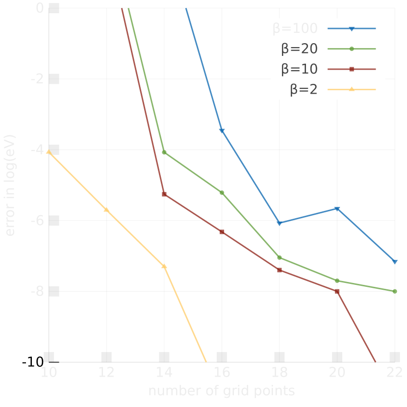
Figure 10: F-grid convergence for GM grand potential SrVO₃. Inverse temperatures are in eV^-1.

The results for different values of $\beta$ of Si and SrVO₃ are given in Fig. 9 and Fig. 10, respectively. One recognizes that the grid convergence is very similar for both systems. Nevertheless, the convergence is worse compared to the RPA, because the F-quadrature error is larger compared to the IA₁-error.

However, our discussion in V.1 suggests that the present choice is the best compromise— at least the best we could find —, and necessitated by the need to have the same time grid for bosonic and fermionic functions, as well as a single frequency grid for fermionic functions. For practical applications, the error of roughly 1 $\mu$eV with 16 and more quadrature points is negligible. Other convergence parameters, such as the energy cutoff of the basis set, typically yield larger errors.Klimeš et al. (2014)

Last, we have considered the electron number conservation of the F-quadrature, that is the difference of $|N_{e}-N^{\prime}_{e}|$, where $N_{e}$ is the exact number of electrons in the unit cell and $N^{\prime}_{e}$ has been calculated from the trace of Equ. (50). We have studied the non-interacting propagator $\tilde{g}$ of Equ. (1) for SrVO₃. This corresponds to roughly $1056\times 64$ poles of the Green’s function on the real-frequency axis in the regime $|x|\leq 400\beta$. The error in the particle number with the number of F-quadrature points is shown in Fig. 11.

Figure 11: Particle number conservation error $|N_{e}-N_{e}^{\prime}|$ of F-grid when calculating the electron density from the non-interacting Kohn-Sham propagator of SrVO₃ (see text). Inverse temperatures are in eV^-1.

One can see that the convergence is exponential and increases and decreases with $\beta$ in the same way as the RPA and GM energies. Not surprisingly, the convergence is the same as compared to the case where the GM energy is used as measure (see Fig. 10). Also, the F-quadrature converges faster with the number of grid points compared to the OHQ-quadrature (not shown). For instance, the F-quadrature yields a precision of $10^{-10}$ states per unit cell for $\beta=10$ using $N=20$ quadrature points, while the same precision is only reached with $N=118$ OHQ-quadrature points.

VIII Conclusion

We presented an efficient method for the Matsubara summation of bosonic and fermionic correlation functions on the imaginary frequency axis. By constructing optimum subspaces of the considered Hilbert space of dimension $N$, we obtained imaginary time and frequency grids for all correlation functions appearing in finite temperature perturbation theory. Furthermore, using the argument of $\varepsilon$-isometric spaces, we have shown that the transformation from imaginary time to imaginary frequency can be performed with high precision.

We implemented this technique in VASP to generalize our zero temperature random phase approximation (RPA) and $GW$ algorithms to finite temperatures and obtained a similar exponential grid convergence for the RPA grand potential (see Fig. 7) as in the $T=0$ case.Kaltak et al. (2014b) To reach $\mu$eV-accuracy, typically, less than 20 grid points are required. This holds true even for low temperatures, so that the RPA grand potential can be evaluated very efficiently for insulating as well as metallic systems with a computational complexity that grows only cubically with the number of electrons in the unit cell.

Furthermore, we showed how to choose the frequency grid for fermionic correlation functions and how to evaluate the Galitskii-Migdal grand potential at finite temperatures using the F-quadrature (see sections IV.1 and V.1). Here a compromise between $\varepsilon$-isometry and integration efficiency has to be made that deteriorates the grid convergence slightly compared to the RPA. For practical applications, however, the precision of the Matsubara summation is still sufficiently good. Other error sources, such as basis set errors will usually dominate.

In summary, we showed that optimized grids can be found for the accurate Matsubara summation of both, bosonic and fermionic functions, with roughly 20 grid points. The hypergeometric grids of OzakiOzaki (2007) and Hu et. al.Hu et al. (2010) (see section III.1) require roughly 100 and more points for the same precision at low temperatures.

Appendix A Second order contribution to the correlation energy at finite $T$

In this appendix, we show that the conserved $L^{2}$-norm of the IA isometry describes the second order contribution to the correlation part of the grand-canonical potential defined in Equ. (12) at finite temperature. We prove this for $\beta=1$ and the diagonal matrix elements $\Omega_{\alpha\gamma}=\sum_{n\in\mathds{Z}}\tilde{\chi}^{2}_{\alpha\gamma}(i\nu_{n})$ using the explicit form for the polarizability in imaginary frequency

$$\begin{split}\tilde{\chi}^{2}_{\alpha\gamma}(i\nu_{n})=&\left[\frac{1}{2}\frac{\Delta_{\alpha\gamma}}{\Delta_{\alpha\gamma}^{2}+\nu_{n}^{2}}\right]^{2}\left[f(x_{\alpha})-f(x_{\gamma})\right]^{2}\\ \Delta_{\alpha\gamma}=&x_{\alpha}-x_{\gamma}.\end{split}$$ (69)

From the series representation of the hyperbolic cotangent (81), and the identity

$$\frac{1}{\left(\Delta_{\alpha\gamma}^{2}+\nu_{n}^{2}\right)^{2}}=\lim_{q\to 0}\frac{1}{2q}\left[\frac{1}{\Delta_{\alpha\gamma}^{2}+\nu_{n}^{2}-q}-\frac{1}{\Delta_{\alpha\gamma}^{2}+\nu_{n}^{2}+q}\right],$$ (70)

and the addition theorem for the hyperbolic tangentAbramowitz and Stegun (1964)

$$\tanh\frac{\Delta_{\alpha\gamma}}{2}=\frac{\tanh\frac{x_{\alpha}}{2}-\tanh\frac{x_{\gamma}}{2}}{1-\tanh\frac{x_{\alpha}}{2}\tanh\frac{x_{\gamma}}{2}}\,,$$ (71)

it is easy to show that

$$\begin{split}\Omega_{\alpha\gamma}=&\frac{1}{4}\left[\frac{f(x_{\alpha})-f(x_{\gamma})}{\tanh\frac{\Delta_{\alpha\gamma}}{2}}\right]^{2}\\ &\times\left[\frac{1}{8}\left(1-\tanh^{2}\frac{\Delta_{\alpha\gamma}}{2}\right)+\frac{1}{4}\frac{\tanh^{2}\frac{\Delta_{\alpha\gamma}}{2}}{\Delta_{\alpha\gamma}}\right].\end{split}$$ (72)

For the sake of simplicity, the Coulomb matrix elements have been suppressed. The last factor in this expression corresponds to the conserved $L^{2}$-norm of the IA₁ isometry in Tab. 1, while the first factor is non-zero for all values of $\Delta_{\alpha\gamma}$ so that the identity $\sum_{n\in\mathds{Z}}\tilde{\chi}^{2}_{\alpha\gamma}(i\nu_{n})=\Omega_{\alpha\gamma}$ can be divided by the same factor proving our assertion. The proof can be generalized to the off-diagonal elements as well.

Appendix B Why frequency grids for GM are difficult

First, we consider the frequency dependence of the free propagator (1). The cosine and sine transformations of the odd and even time basis functions (39) and (38) for fermionic frequencies (5) are given in Eqs. (21) and (22), respectively. Then the non-interacting propagator (1) on the fermionic Matsubara axis reads

$$\tilde{g}(x_{\alpha},i\omega_{m})=\tilde{u}_{\omega_{m}}(x_{\alpha})+i\tilde{v}_{\omega_{m}}(x_{\alpha}).$$ (73)

Second, we observe that every fermionic function can be decomposed into terms that are even and odd in $\omega$, including the product of the propagator and self-energy as it appears in the GM grand potential (13). It is, obvious, that only the real part of the product $\tilde{G}\tilde{\Sigma}$ contributes to the total energy. Thus the most general matrix element, which gives a non-zero contribution to the GM grand potential has the form

$$\begin{split}\tilde{G}(i\omega_{m})\tilde{\Sigma}(i\omega_{m})=&\sum\limits_{-x_{\max}\leq x,y\leq x_{\max}}D_{G}(x)D_{\Sigma}(y)\\ \times&\left[\tilde{u}_{\omega_{m}}(x)\tilde{u}_{\omega_{m}}(y)-\tilde{v}_{\omega_{m}}(x)\tilde{v}_{\omega_{m}}(y)\right],\end{split}$$ (74)

where $x$ and $y$ are the poles of the Green’s function and the self-energy on the real-frequency axis and $D_{G},D_{\Sigma}$ the spectral densities, respectively. Without loss of generality, we set $D_{G}=D_{\Sigma}=1$ and assume that the magnitudes of the poles are smaller than a positive number, i.e. $|x|,|y|\leq x_{\max}$. Third, we note that the analogue of the IA₁-quadrature of bosonic functions (45) for fermionic ones

$$\min_{\sigma_{k}>0,\omega_{k}\in(0,\infty)}\max_{0\leq x\leq x_{\rm max}}\left|\|x\|^{2}_{2}-\sum\limits_{k=1}^{N}\sigma_{k}\tilde{u}^{2}_{k}(x)\right|$$ (75)

yields the IB₁-quadrature, see Tab. 1. Unfortunately, the IB₁-quadrature only allows to evaluate the first term on the right hand side of (74) accurately, but fails for the product of two odd functions $\tilde{v}$. Similarly, the IA₂-quadrature obtained from the minimax problem

$$\min_{\sigma_{k}>0,\omega_{k}\in(0,\infty)}\max_{0\leq x\leq x_{\rm max}}\left|\|x\|^{2}_{2}-\sum\limits_{k=1}^{N}\sigma_{k}\tilde{v}^{2}_{k}(x)\right|$$ (76)

that approximates the same norm as the time and IA₁-quadrature, describes only the second term in (74). Consequently, neither the IB₁- nor the IA₂-quadrature can be used for our purposes.

Appendix C Poisson summation and hyperbolic functions: A proof of Equ. (47)

To proof identity (47), we use Poissons summation formulaHiggins (1985)

$$\sum\limits_{n\in\mathds{Z}}f(n)=\sum\limits_{k\in\mathds{Z}}\tilde{f}(k)$$ (77)

for a function $f$ and its Fourier transform $\tilde{f}$. Inserting $f(tz)=e^{-2|tz|}$ into the left hand side of (77) one obtains with the geometric series of the hyperbolic cotangent

$$\sum\limits_{n\in\mathds{Z}}e^{-2|nz|}=\frac{1+e^{-2|z|}}{1-e^{-2|z|}}=\coth|z|.$$ (78)

Consequently, evaluating the Fourier integral gives

$$\tilde{f}(k)=\int_{-\infty}^{\infty}\mathrm{d}te^{-2|tz|}e^{i2\pi kt}=\frac{|z|}{\pi^{2}k^{2}+|z|^{2}},$$ (79)

which after inserting into the right hand side of (77) yields the identity

$$\coth|z|=\sum\limits_{k\in\mathds{Z}}\frac{|z|}{\pi^{2}k^{2}+|z|^{2}}.$$ (80)

On the one hand, replacing $|z|\to|z|/2$ and dividing by $2$, this identity becomes

$$\frac{1}{2}\coth\frac{|z|}{2}=\sum\limits_{k\in\mathds{Z}}\frac{|z|}{(\pi 2k)^{2}+|z|^{2}}.$$ (81)

On the other hand, the series (80) on the right hand side can be split into a series over even and a series over odd integers

$$\coth|z|=\underbrace{\sum\limits_{k\in\mathds{Z}}\frac{|z|}{(\pi 2k)^{2}+|z|^{2}}}_{=\frac{1}{2}\coth\frac{|z|}{2}}+\sum\limits_{k\in\mathds{Z}}\frac{|z|}{(\pi(2k+1))^{2}+|z|^{2}}$$ (82)

The first term on the right hand side follows from (81), while the second part is the left hand side of Equ. (47). After comparison with the well-known hyperbolic identity

$$\coth z=\frac{1}{2}\coth\frac{z}{2}+\frac{1}{2}\tanh\frac{z}{2},$$ (83)

one identifies the second term in (82) with

$$\frac{1}{2}\tanh\frac{|z|}{2}=\sum\limits_{k\in\mathds{Z}}\frac{|z|}{(\pi(2k+1))^{2}+|z|^{2}}$$ (84)

and Equ. (47) is proven.

Note, the derivative of the left and right hand side of Eqs. (84) and (81) in combination with the q-analog (70) gives an alternative way to calculate the $L^{2}$-norms tabulated in Tab. 1.

References

- Mermin (1965) N. D. Mermin, Phys. Rev. 137, A1441 (1965).
- Fu and Ho (1983) C.-L. Fu and K.-M. Ho, Phys. Rev. B 28, 5480 (1983).
- De Vita and Gillan (1991) A. De Vita and M. Gillan, J. Phys. Condens. Matter 3, 6225 (1991).
- Methfessel and Paxton (1989) M. Methfessel and A. Paxton, Phys. Rev. B 40, 3616 (1989).
- Kresse and Furthmüller (1996) G. Kresse and J. Furthmüller, Phys. Rev. B 54, 11169 (1996).
- Kohn and Luttinger (1960) W. Kohn and J. M. Luttinger, Phys. Rev. 118, 41 (1960).
- Luttinger and Ward (1960) J. M. Luttinger and J. C. Ward, Phys. Rev. 118, 1417 (1960).
- Matsubara (1955) T. Matsubara, Prog. Theor. Exp. Phys. 14, 351 (1955).
- Fetter and Walecka (2003) A. L. Fetter and J. D. Walecka, Quantum theory of many-particle systems, Dover Books on Physics (Dover Publications, 2003).
- Negele and Orland (1988) J. Negele and H. Orland, Quantum many-particle systems, Frontiers in physics (Addison-Wesley Pub. Co., 1988).
- Rojas et al. (1995) H. N. Rojas, R. W. Godby, and R. J. Needs, Phys. Rev. Lett. 74, 1827 (1995).
- Rieger et al. (1999) M. M. Rieger, L. Steinbeck, I. D. White, H. N. Rojas, and R. W. Godby, Comput. Phys. Commun. 117, 211 (1999), arXiv:9805246 [cond-mat] .
- Kaltak et al. (2014a) M. Kaltak, J. Klimeš, and G. Kresse, Phys. Rev. B 90, 054115 (2014a).
- Kaltak et al. (2014b) M. Kaltak, J. Klimeš, and G. Kresse, J. Chem. Theory Comput. 10, 2498 (2014b).
- Faleev et al. (2006) S. V. Faleev, M. van Schilfgaarde, T. Kotani, F. Léonard, and M. P. Desjarlais, Phys. Rev. B 74, 033101 (2006).
- Ku and Eguiluz (2002) W. Ku and A. G. Eguiluz, Phys. Rev. Lett. 89, 126401 (2002).
- Welden et al. (2016) A. R. Welden, A. A. Rusakov, and D. Zgid, J. Chem. Phys. 145, 204106 (2016).
- Boehnke et al. (2011) L. Boehnke, H. Hafermann, M. Ferrero, F. Lechermann, and O. Parcollet, Phys. Rev. B 84, 075145 (2011).
- Huang (2016) L. Huang, Chin. Phys. B 25, 117101 (2016).
- Ozaki (2007) T. Ozaki, Phys. Rev. B 75, 035123 (2007).
- Hu et al. (2010) J. Hu, R.-X. Xu, and Y. Yan, J. Chem. Phys. 133, 101106 (2010).
- Shinaoka et al. (2017) H. Shinaoka, J. Otsuki, M. Ohzeki, and K. Yoshimi, Phys. Rev. B 96, 035147 (2017).
- Li et al. (2020) J. Li, M. Wallerberger, N. Chikano, C.-N. Yeh, E. Gull, and H. Shinaoka, Phys. Rev. B 101, 035144 (2020).
- Remez (1962) E. I. A. Remez, General computational methods of Chebyshev approximation: The Problems with Linear Real Parameters (U. S. Atomic Energy Commission, Division of Technical Information, 1962).
- Takatsuka et al. (2008) A. Takatsuka, S. Ten-No, and W. Hackbusch, J. Chem. Phys. 129, 044112 (2008).
- Häser and Almlöf (1992) M. Häser and J. Almlöf, J. Chem. Phys. 96, 489 (1992).
- Wick (1954) G. C. Wick, Phys. Rev. 96, 1124 (1954).
- Osterwalder and Schrader (1973) K. Osterwalder and R. Schrader, Comm. Math. Phys. 31, 83 (1973).
- Osterwalder and Schrader (1975) K. Osterwalder and R. Schrader, Comm. Math. Phys. 42, 281 (1975).
- (30) F. W. J. Olver, A. B. Olde Daalhuis, D. W. Lozier, B. I. Schneider, R. F. Boisvert, C. W. Clark, B. R. Miller, and B. V. Saunders, “NIST digital library of mathematical functions,” .
- Liu et al. (2016) P. Liu, M. Kaltak, J. Klimeš, and G. Kresse, Phys. Rev. B 94, 165109 (2016).
- Gell-Mann and Brueckner (1957) M. Gell-Mann and K. A. Brueckner, Phys. Rev. 106, 364 (1957).
- Bohm and Pines (1951) D. Bohm and D. Pines, Phys. Rev. 82, 625 (1951).
- Pines and Bohm (1952) D. Pines and D. Bohm, Phys. Rev. 85, 338 (1952).
- Bohm and Pines (1953) D. Bohm and D. Pines, Phys. Rev. 92, 609 (1953).
- Galitskii and Migdal (1958) V. M. Galitskii and A. B. Migdal, Zh. Eksp. Teor. Fiz. 34, 139 (1958).
- Caruso et al. (2013) F. Caruso, D. R. Rohr, M. Hellgren, X. Ren, P. Rinke, A. Rubio, and M. Scheffler, Phys. Rev. Lett. 110, 146403 (2013).
- Hedin (1965) L. Hedin, Phys. Rev. 139, A796 (1965).
- Grumet et al. (2018) M. Grumet, P. Liu, M. Kaltak, J. Klimeš, and G. Kresse, Phys. Rev. B 98, 155143 (2018).
- Note (1) The isometry (29\@@italiccorr) is known as Parseval theoremvon Querenburg (2013) or, if is continuous, Plancherel theorem for Fourier transforms.Plancherel (1910).
- Fleming and Jamison (2002) R. Fleming and J. Jamison, Isometries on Banach Spaces: function spaces (CRC Press, 2002).
- Ding (1988) G. Ding, Acta Math. Sci. 8, 361 (1988).
- Braess (1986) D. Braess, Nonlinear Approximation Theory (Springer-Verlag, 1986).
- von Querenburg (2013) B. von Querenburg, Mengentheoretische Topologie (Springer Berlin Heidelberg, 2013).
- Axler et al. (1999) S. Axler, H. Schaefer, M. Wolff, M. Wolff, F. Gehring, and K. Ribet, Topological Vector Spaces (Springer New York, 1999).
- Braess and Hackbusch (2005) D. Braess and W. Hackbusch, IMA J. Numer. Anal. 25, 685 (2005).
- Golub and Pereyra (2003) G. Golub and V. Pereyra, Inverse Probl. 19, R1 (2003).
- Hammerlin and Hoffmann (1994) G. Hammerlin and K. Hoffmann, Numerische Mathematik (Springer Berlin Heidelberg, 1994).
- Press et al. (2007) W. H. Press, S. A. Teukolsky, W. T. Vetterling, and B. P. Flannery, Numerical Recipes 3rd Edition (Cambridge University Press, 2007).
- Kresse and Joubert (1999) G. Kresse and D. Joubert, Phys. Rev. B 59, 1758 (1999).
- Feynman (1948) R. P. Feynman, Rev. Mod. Phys. 20, 367 (1948).
- Stueckelberg (1941) E. C. G. Stueckelberg, Helv. Phys. Acta. 14, 322 (1941).
- Levinstein et al. (1999) M. Levinstein, S. Rumyantsev, and M. Shur, Handbook Series on Semiconductor Parameters (World Scientific, London, 1999).
- Onoda et al. (1991) M. Onoda, H. Ohta, and H. Nagasawa, Solid State Commun. 79, 281 (1991).
- Klimeš et al. (2014) J. Klimeš, M. Kaltak, and G. Kresse, Phys. Rev. B 90, 075125 (2014).
- Perdew et al. (1996) J. P. Perdew, M. Ernzerhof, and K. Burke, J. Chem. Phys. 105, 9982 (1996).
- Gajdoš et al. (2006) M. Gajdoš, K. Hummer, G. Kresse, J. Furthmüller, and F. Bechstedt, Phys. Rev. B 73, 045112 (2006).
- Harl and Kresse (2008) J. Harl and G. Kresse, Phys. Rev. B 77, 045136 (2008).
- Helmich-Paris and Visscher (2016) B. Helmich-Paris and L. Visscher, J. Comput. Phys. 321, 927 (2016).
- Beuerle et al. (2018) M. Beuerle, D. Graf, H. F. Schurkus, and C. Ochsenfeld, J. Chem. Phys. 148, 204104 (2018).
- Note (2) Fixing this requires the adjustment of the chemical potential and re-calculation of the interacting Green’s function until is satisfied.
- Abramowitz and Stegun (1964) M. Abramowitz and I. A. Stegun, Handbook of Mathematical Functions with Formulas, Graphs, and Mathematical Tables (Dover, New York, 1964).
- Note (3) The imaginary part is proportional to odd terms in the frequency and vanishes when the sum over all (positive and negative) fermionic Matsubara frequencies is carried out.
- Higgins (1985) J. R. Higgins, Bull. Amer. Math. Soc. (N.S.) 12, 45 (1985).
- Plancherel (1910) M. Plancherel, Rend. Circ. Mat. Palermo 30, 289 (1910).