Longitudinal correlations from fluctuating strings in Pb-Pb, p-Pb, and p-p collisions

Abstract

In a framework of a semi-analytic model with longitudinally extended strings of fluctuating end-points, we demonstrate that the rapidity spectra and two-particle correlations in collisions of Pb-Pb, p-Pb, and p-p at the energies of the Large Hadron Collider can be universally reproduced. In our approach, the strings are pulled by wounded constituents appearing in the Glauber modeling at the partonic level. The obtained rapidity profile for the emission of hadrons from a string yields bounds for the distributions of the end-point fluctuations. Then, limits for the two-particle-correlations in pseudorapidity can be obtained. Our results are favorably compared to recent experimental data from the ATLAS Collaboration.

I Introduction

Longitudinal correlations are an important source of information on the dynamics of hadronic collisions. There are numerous on-going efforts to understand them, both at the theoretical side, as well as in the experiments at BNL Relativistic Heavy-Ion Collider (RHIC) and the CERN Large Hadron Collider (LHC), in particular with detector upgrades covering broader ranges in pseudorapidity. As is well known, the long-range rapidity correlations supply information on the earliest phases of the reaction, since from causality the correlations stem from proper times $\tau$ limited by $\tau\lesssim\tau_{f}\exp(-\Delta\eta/2)$, where $\tau_{f}$ is the freeze-out proper time and $\Delta\eta$ is the pseudorapidity separation of the particles in the pair.

In our recent paper Rohrmoser:2018shp we have presented an analysis of the longitudinal hadronic correlations at the highest RHIC energy of $\sqrt{s_{\rm NN}}=200$ GeV in the framework of a simple model, where emission proceeds from strings with fluctuating end-points Broniowski:2015oif . The model is, up to emission profiles extracted from the data, analytic, which allows us for a simple understanding of generic production features present in various string or fluxtube approaches. The present study provides an extension of our method to the LHC energies.

We recall that QCD-motivated string or color flux-tube models are commonly used in particle physics phenomenology to describe the longitudinal dynamics. The strings extend between receding color sources and fragment, producing hadrons. Many sophisticated Monte Carlo codes are based on the Lund string model (see, e.g., Andersson:1983ia ; Wang:1991hta ; Lin:2004en ; Sjostrand:2014zea ; Bierlich:2018xfw ; Ferreres-Sole:2018vgo ), or on the Dual Parton Model build on the Pomeron and Regge exchanges Capella:1992yb ; Werner:2010aa ; Pierog:2013ria . A common feature of these phenomenologically successful codes is a formation of a collection of strings pulled between the constituents of the projectiles in the early stage of the collision. The end-points of a string have opposite color charges (triplet-antitriplet for the quark-diquark and quark-antiquark configurations, or octet-octet for the gluon-gluon case). Moreover, the location of the string end-points in spatial rapidity $\eta_{PS}\equiv\tfrac{1}{2}\ln[(t+z)/(t-z)]$ fluctuates following a proper parton distribution function. As argued in Broniowski:2015oif ; Rohrmoser:2018shp , these fluctuations are the key feature enabling control over the one body densities (pseudorapidity spectra) and the two-particle correlations in pseudorapidity. In our study we focus on this effect, neglecting other features typically incorporated in Monte Carlo codes, such as the nuclear shadowing or baryon stopping. In our study, rather than using the parton distribution functions to describe the end-point distributions, we take a more flexible and phenomenological approach, where these distributions are adjusted to reproduce the pseudorapidity spectra.

Another important issue is the distribution of the number of strings, which finally translates into the multiplicity of the produced hadrons. We use the fact that the multiplicity of the produced hadrons is successfully described within the wounded picture Bialas:1976ed , which is an adoption of the Glauber theory Glauber:1959aa to inelastic collisions Czyz:1969jg . Moreover, the wounded quark scaling Bialas:1977en ; Bialas:1977xp ; Bialas:1978ze ; Anisovich:1977av has been shown to work surprisingly well Eremin:2003qn ; KumarNetrakanti:2004ym ; Bialas:2006kw ; Bialas:2007eg ; Alver:2008aq ; Agakishiev:2011eq ; Adler:2013aqf ; Loizides:2014vua ; Adare:2015bua ; Lacey:2016hqy ; Bozek:2016kpf ; Zheng:2016nxx ; Sarkisyan:2016dzo ; Mitchell:2016jio ; Chaturvedi:2016ctn ; Loizides:2016djv ; Tannenbaum:2017ixt ; Barej:2017kcw ; Barej:2019xef at both RHIC and the LHC collision energies. Extensions to more partons per nucleon than just three quarks have also been considered, with the conclusion that the increase in energy yields more wounded partons Bozek:2016kpf . In the present study we use the wounded model with a few (3 to 6) constituents per nucleon.

II The model

As mentioned, our model combines the string picture with the wounded parton model, assuming that the number of strings is given by the number of the wounded constituents. As a matter of fact, this complies to the Lund model mechanism, where the basic string extends between a parton from a given nucleon and a parton (or diquark) from the same nucleon Andersson:1983ia . Thus, in collisions of nuclei $A$ and $B$, hadrons are emitted from strings associated to mutually independent $N_{A}$ wounded partons from $A$ and $N_{B}$ wounded partons from $B$, respectively. At a given collision energy the emission profile of hadrons (defined as the number of hadrons per $\eta$) from each string, $f(\eta)$, is assumed to be universal, i.e., independent of the mass numbers of the projectiles or centrality. Here $\eta$ denotes the pseudorapidity in the center of mass of the colliding NN system. The above assumptions correspond to the following scaling law Bialas:2004su :

$$\frac{dN_{\rm ch}}{d\eta}=\langle N_{A}\rangle f(\eta)+\langle N_{B}\rangle f(-\eta),$$ (1)

where we have adopted the convention that $A$ moves to the right and $B$ to the left along the $z$ axis. The symbol $\langle.\rangle$ denotes the average over events in the considered centrality class.

From Eq. (1) it follows that the symmetric and antisymmetric parts of the distributions are given by

$$\frac{1}{2}\left(\frac{dN}{d\eta}(\eta)+\frac{dN}{d\eta}(-\eta)\right)=\langle N_{+}\rangle f_{s}(\eta),$$

$$\frac{1}{2}\left(\frac{dN}{d\eta}(\eta)-\frac{dN}{d\eta}(-\eta)\right)=\langle N_{-}\rangle f_{a}(\eta),$$ (2)

with $N_{\pm}=N_{A}\pm N_{B}$ denoting the sum and the difference of sources from $A$ and $B$, whereas $f_{s}(\eta)$ and $f_{a}(\eta)$ denote the symmetric and antisymmetric parts of the profile $f(\eta)$.

In our simulations, centrality is determined via the quantiles of the total number of wounded partons, $\langle N_{+}\rangle$.

From various studies of hadron multiplicity distributions in p-Pb collisions, it is known that the Glauber approach of hadron production must be amended with fluctuations of the number of sources. Typically, the negative binomial distribution is overlaid over the distribution of wounded sources. We follow this scheme in our simulations, with the following prescription: we generate events with GLISSANDO 3 Bozek:2019wyr , with $n_{A}$ and $n_{B}$ wounded partons in a given event. Then we generate randomly $N_{A}=k(N_{A};n_{A},q)$ and $N_{B}=k(N_{B};n_{B},q)$, where

$$k(x;n,q)={\rm NB}\left[x;\frac{nq}{1-q},q\right]$$ (3)

is the negative binomial distribution with $x=0$ removed, i.e., $x=1,2,3,\dots$. The cases where $N_{A}=0$ or $N_{B}=0$ (no strings) are disregarded. By construction, $\langle x\rangle=n$ and ${\rm var}(x)=n/q$. The parameter $q\leq 1$, treated as a free variable to be fitted, controls the variance of the number of strings.

The role of increased fluctuations introduced by an overlaid distribution enters indirectly into our analysis, by modifying the division of the event sample into centrality classes.

III Extraction of the emission profile from pseudorapidity spectra

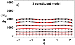
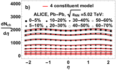
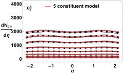
Figure 1: Model results (solid lines) and ALICE data Adam:2016ddh (points with bands indicating experimental errors) for the pseudorapidity spectra in Pb-Pb collisions at $5.02$ TeV. Subsequent panels correspond to models with 3, 4, 5, and 6 partons per nucleon.

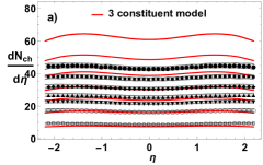
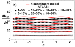
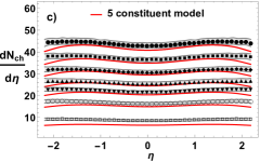
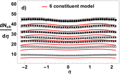
Figure 2: Model results (solid lines) and ATLAS data Aad:2015zza (points with bands indicating experimental errors) for the symmetric parts of the pseudorapidity spectra in p-Pb collisions at $5.02$ TeV. Subsequent panels correspond to models with 3, 4, 5, and 6 partons per nucleon.

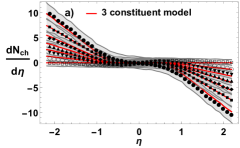
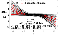
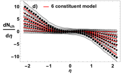
Figure 3: Same as in Fig. 2, but for the antisymmetric part of the p-Pb spectra.

This section explains in detail how the experimental data on rapidity spectra from p-Pb and Pb-Pb collisions at the LHC with $\sqrt{s_{\rm NN}}=5.02$ TeV were jointly fitted to obtain the emission profiles of Eq. (1). We carry out the following steps:

1. Choose the variant of the model by deciding on the number of partons per nucleon.

2. GLISSANDO 3 is run to generate event samples with the number of wounded sources $n_{A}$ and $n_{B}$ for both the p-Pb and Pb-Pb collisions.

3. For a given value of $q$ samples with string numbers $N_{A}$ and $N_{B}$ are obtained by overlaying a negative binomial distribution according to Eq. (3).

4. The samples for p-Pb and Pb-Pb are then divided into centrality classes according to the values of $N_{+}$.

5. The values of $\langle N_{A}\rangle$ and $\langle N_{B}\rangle$ in all centrality classes are used to construct the least squares fit of the profiles $f(\eta)$ to the experimental pseudorapidity spectra ${dN_{\rm ch}}/{d\eta}$ from Eq. (1).

6. Steps 3-5 are repeated to obtain the optimum value of $q$, corresponding to a global minimum of the least square function. The result is the optimum profile $f(\eta)$.

In the fitting procedure, the symmetric part of the profile, $f_{s}(\eta)$, is sensitive to both the Pb-Pb and p-Pb data, whereas the the antisymmetric part, $f_{a}(\eta)$, depends only on the (asymmetric) p-Pb collisions, as is obvious from Eq. (2) As we wish to fit jointly the Pb-Pb and p-Pb, we choose the collision energy where both sets of data on the pseudorapidity spectra are available, namely $\sqrt{s_{NN}}=5.02$ TeV. Specifically, we take ALICE data Adam:2016ddh on pseudorapidity spectra of Pb-Pb, and the ATLAS data Aad:2015zza on pseudorapidity spectra of p-Pb. We note that the used data for the p-Pb pseudorapidity spectra for p-Pb collisions from ATLAS Aad:2015zza are accurately compatible to the ALICE Adam:2016ddh data with the V0A selection of centrality. We prefer to use the ATLAS data here, as we will compare the results of our model with the pseudo-rapidity correlations extracted from the ATLAS-experiment Aad:2015zza .

The experimental data for p-Pb collisions at the LHC are shifted with respect to the NN center-of-mass frame by 0.465 units of rapidity. Since rapidity $y$ and pseudorapidity $\eta$ are related as $p_{T}\sinh(\eta)=\sqrt{m^{2}+p_{T}^{2}}\sinh(y)$, where $p_{T}$ is the transverse momentum and $m$ the particle’s mass, one can obtain $\eta\approx y$ in the case $m\ll p_{T}$, which we assume in our further considerations. One can justify this assumption by the fact that the emitted particles are predominantly pions with a small rest mass of $m_{\pi}\simeq 140$ MeV, which is smaller than typical values of $p_{T}$. Thus, to a good approximation the pseudorapidity $\eta$ in the lab frame is related to $\eta$ in the NN center-of-mass frame, $\eta_{\rm lab}\simeq\eta_{\rm CM}+0.465$. This allows us to transform the experimental pseudorapidity spectra from p-Pb collisions into the CM frame by a simple shift.

A joint least squares fit for Pb-Pb and p-Pb spectra can be performed in the following way: For each value of $q$ individually the numbers of sources in the wounded parton model, overlaid with the negative binomial distribution, are generated with the help of GLISSANDO 3 Bozek:2019wyr . In order to obtain the emission profile $f(\eta)$ we construct for each value of $\eta$ for which the data exists the least squares sum $L(f_{A}(\eta),f_{B}(\eta))$, depending on two fitting parameters $f_{A}(\eta)$ and $f_{B}(\eta)$,

$$L(f_{A}(\eta),f_{B}(\eta))=$$ (4)

$$\frac{1}{N}\sum_{i=1}^{N}\left\{\left[\left(\frac{dN}{d\eta}(\eta)\right)_{i}-(\langle N_{A}\rangle_{i}f_{A}(\eta)+\langle N_{B}\rangle_{i}f_{B}(\eta))\right]^{2}\right.$$

$$+\left.\left[\left(\frac{dN}{d\eta}(-\eta)\right)_{i}-(\langle N_{B}\rangle_{i}f_{A}(\eta)+\langle N_{A}\rangle_{i}f_{B}(\eta))\right]^{2}\right\},$$

where $i$ runs over all spectra (i.e., all the centrality classes and reactions) that are to be fitted. We then minimize $L(\eta,f_{A},f_{B})$ at each $\eta$, which yields the functions $f_{A}(\eta)$ and $f_{B}(\eta)$. Our choice for the least squares sum, Eq. (4), has the desired symmetry property $L(-\eta,f_{A},f_{B})=L(\eta,f_{B},f_{A})$, which follows from the fact that $f_{A}(\eta)=f_{B}(-\eta)$, which means the replacement of the left-going wounded source by the right-going one. Recall that in the notation of Eq. (1) $f(\eta)=f_{A}(\eta)=f_{B}(-\eta)$.

Table 1: Optimum values of the negative binomial parameter $q$ and the corresponding value of the least squares function $\hat{L}$, for models with various numbers of partons per nucleon.

constituents	$q$	$\tilde{L}$
3	0.245	476
4	0.905	140
5	0.785	137
6	0.805	571

The procedure described above provides the optimum emission spectrum $f(\eta)$ for a given value of the negative binomial parameter $q$ of Eq. (3) . To obtain the optimum value of $q$ we additionally minimize the least squares sum (4) summed over all values of $\eta$, denoted as $\hat{L}$, with respect to $q$. The optimum values for $q$ for the models with 3, 4, 5, and 6 partons per nucleon together with the corresponding value for the least squares sum $\tilde{L}$ are listed in Table 1. We note that the values for $\tilde{L}$ are lowest for models with $4$ or $5$ constituents per nucleon. Thus in the following we focus on results for these two cases.

The results of our fits for the symmetric parts of the Pb-Pb pseudorapidity spectra for the models with 3, 4, 5, and 6 partons per nucleon are shown in Fig. 1. As the figure shows, the ALICE data Adam:2016ddh are reasonably well reproduced for all variants of the model and for all centrality selections. Thus the Pb-Pb spectra do not discriminate between the variants of the model.

The situation is different for the p-Pb case. Figures 2 and 3 show, correspondingly, the symmetric and antisymmetric parts of the pseudorapidity spectra for p-Pb collisions, compared the ATLAS data Aad:2015zza . Whereas for the antisymmetric contributions, shown in Fig. 3, all variants of the model reproduce the data reasonably well, significant differences can be noticed in the symmetric contributions, shown in Fig. 2. Acceptable agreement is obtained for $4$ and $5$ partons. In the following parts of this article, when considering correlations, we will thus focus on the $4$ and $5$ parton cases.

The corresponding universal profiles $f(\eta)$ obtained from our fitting procedure are shown in Fig. 4, together with their symmetric and antisymmetric contributions $f_{s}(\eta)$ and $f_{a}(\eta)$ given in Fig. 5. We note from Fig. 4 that the profiles scaled by the central value, $f(\eta)/f(0)$, differ by a few percent at peripheral values of $\eta$, with a steeper the fall-off with $\eta$ for larger number of partons per nucleon.

Figure 5a) shows that the symmetric parts of the profiles, $f_{s}(\eta)$, decrease with the number of partons. This behavior is natural and follows from the first of Eq. (2). When $\langle N_{+}\rangle$ decreases due to a smaller number of partons per nucleon, the magnitude of $f_{s}(\eta)$ needs to be correspondingly increased to yield the same pseudorapidity spectra. Figure 5b) shows the antisymmetric parts of the profiles, $f_{a}(\eta)$. As can be seen, the different number of partons per nucleon has essentially no influence on the $f_{a}(\eta)$. We have found no apparent physical reason for such a behavior, which may be considered accidental. The overall steeper fall-off of profiles $f(\eta)/f(0)$ in Fig. 4 with increasing number of partons per nucleon can thus be understood via the decrease of the magnitude of $f_{s}(\eta)$, with no change in $f_{a}(\eta)$.

We remark that instead of the least squares sum of Eq. (4) we can use the $\chi^{2}$ function, which yields essentially the same optimum results. As to the values of $\chi^{2}$/d.o.f., admittedly they are large due to the approximate nature of our model, which assumes a very simple uniform mechanism of string production and breaking. Thus the values of $\chi^{2}$/d.o.f. cannot be used as stringent measures of the statistical quality of the fit, which is an issue shared by many models applied to ultra-relativistic nuclear collisions.

To conclude this section, as a preliminary step of our study we were able to uniformly fit in an approximate way the experimental data for Pb-Pb and p-Pb collision from the ALICE Adam:2016ddh and ATLAS Aad:2015zza collaborations, respectively, in the wounded parton model, with a preference for a model variant with 4 or 5 wounded constituents per nucleon.

IV String end point distributions

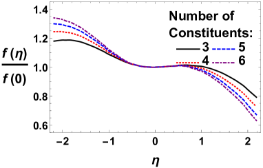
Figure 4: Emission profile in pseudorapidity, divided by its value at the origin, $f(\eta)/f(0)$, for models with various number of constituents per nucleon.

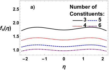
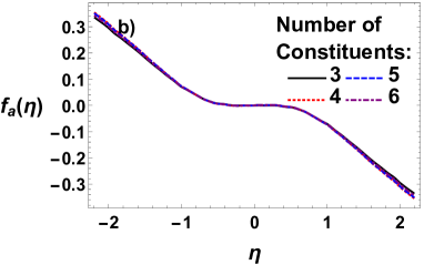
Figure 5: Symmetric (a) and antisymmetric (b) parts of the emission profile $f(\eta)$ for models with various number of constituents per nucleon.

In this section we proceed in analogy to our earlier work Rohrmoser:2018shp . However, in contrast to the description used therein, in this article we pass from the profile functions in pseudorapidity $\eta$, obtained in the previous section, to the profile functions in rapidity $y$. The reason is technical but relevant. The method of Rohrmoser:2018shp works for profile functions with are unimodal (have a single maximum), as this is what follows from strings continuously stretched between fluctuating end-points. Unimodality is not the case in the present analysis, as can be seen from Fig. 4. For instance, for the case of three constituent partons per nucleon, one can notice a maximum at $\eta\simeq-1.8$ and another weak maximum at $\eta\simeq 0.8$ (variants with a larger number of constituents have a maximum outside of the left bound of the plot). However, the maximum near 0.8 is an artifact of using pseudorapidity rather than rapidity.

As can be seen from the experimental data Back:2001xy ; Adam:2014qja ; Aad:2015zza ; Adam:2016ddh , pseudorapidity spectra mainly differ from rapidity spectra by a pronounced dip around $\eta=0$, which trivially follows from the kinematic relation between rapidity and pseudorapidity. In order to pass from pseudorapidity to rapidity for the spectra which are largely dominated by the pions, we use the simplifying assumption of a factorization of the rapidity and $p_{T}$ dependence of the spectra. Then, approximately, one can write

$$\frac{dN}{dy}=\int dp_{T}\frac{d\eta(y,p_{T},m_{\pi})}{dp_{T}dy}\frac{dN}{d\eta}\approx\left.\frac{d\eta}{dy}\frac{dN}{d\eta}\right|_{y\approx\eta}\,.$$ (5)

The Jacobian ${d\eta}/{dy}$ in the last part of Eq. (5) can be obtained from the experimental data from ALICE for the $5\%$ most central Pb-Pb collisions Adam:2016ddh , where both the rapidity, $dN/dy$, and pseudorapidity, $dN/d\eta$, spectra are provided. This procedure, in essence, is a way of averaging over the transverse momentum $p_{T}$, incorporating the experimental acceptance.

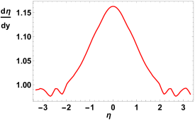
Figure 6: The Jacobian $d\eta/dy$ obtained from Eq. 6 and the experimental data from Adam:2016ddh .

Consequently, we can obtain the one-body emission profiles $f(y)$ in terms of $f(\eta)$ presented in Sec. III, namely,

$$f(y)=\frac{d\eta}{dy}f(\eta).$$ (6)

Thus obtained result for $d\eta/dy$ is shown in Fig. 6. Similarly, for the two-particle emission profiles we get

$$f_{2}(y_{1},y_{2})=\frac{d\eta_{1}}{dy_{1}}\frac{d\eta_{2}}{dy_{2}}f_{2}(\eta_{1},\eta_{2}),$$ (7)

which will be used in the next section.

The results for $f(y)$ in models with 3, 4, 5, and 6 wounded partons obtained with Eq. (6) are shown in Fig. 7. The feature that can be seen when comparing to $f(\eta)$ from Fig. 4 is the absence of the central dip in the symmetric part. As a result, $f(y)$ at various centralities are unimodal functions (have only one maximum at negative $y$), which allows to carry out the analysis along the lines of Rohrmoser:2018shp . We recapitulate the basic steps of the procedure:

1. Each of the $N_{A}$ and $N_{B}$ wounded sources is associated to a longitudinally extended string.

2. A string breaking at spatial rapidity $y$ corresponds to a particle emission at rapidity $y$. The corresponding probability distribution for string breaking, $s(y;y_{1},y_{2})$, is uniform between the end-points $y_{1}$ and $y_{2}$, namely $s(y;y_{1},y_{2})=\omega(\theta(y_{1}<y<y_{2})+\theta(y_{2}<y<y_{1}))$, where $\omega$ is a normalization constant and the function $\theta$ equals $1$ wherever the condition in its argument is fulfilled, and $0$ otherwise.

3. String-end points $y_{1}$ and $y_{2}$ follow distributions $g_{1}(y_{1})$ and $g_{2}(y_{2})$, respectively. The corresponding cumulative distribution functions (CDFs) are denoted as $G_{1}(y_{1})$ and $G_{2}(y_{2})$.

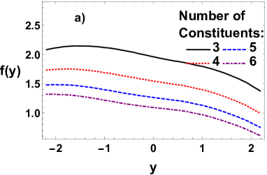
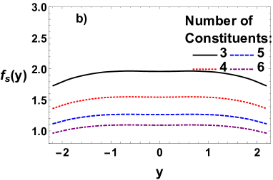
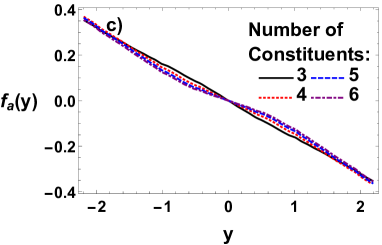
Figure 7: Emission profiles of individual strings in rapidity for models with various numbers of wounded constituents (a) together with their respective symmetric (b) and antisymmetric parts (c).

Then, the one-body emission profile $f(y)$ can be written as Rohrmoser:2018shp

$$f(y) =\int_{-\infty}^{\infty}dy_{1}\int_{-\infty}^{\infty}dy_{2}g_{1}(y_{1})g_{2}(y_{2})s(y;y_{1},y_{2})$$

$$=\omega\left\{\tfrac{1}{2}-2[G_{1}(y)-\tfrac{1}{2}][G_{2}(y)-\tfrac{1}{2}]\right\}.$$ (8)

It is apparent from Eq. (8) that for a given one-body emission profile the solution to the string-end-point distributions $G_{1}(y)$ and $G_{2}(y)$ are not unique. It is, nevertheless, possible to constrain the range of possible solutions for the CDFs Rohrmoser:2018shp . We denote $y_{0}$ as the position of the maximum of $f(y)$, and consider the two extreme cases:

1. $f(y_{0})={\omega}/{2}$: In that case the string-end-point distributions $g_{1}(y)$ and $g_{2}(y)$ for both ends of the strings are identical. We label this case as “$g_{1}=g_{2}$”. Of course, in this case also $G_{1}(y)=G_{2}(y)$.

2. $f(y_{0})=\omega$: In this case, the supports for the string-end-point distributions $g_{1}(y)$ and $g_{2}(y)$ in rapidity are disjoint, hence we refer to this case as the “disjoint case”. The distribution of the left end-point, $g_{1}$, has support for $y\leq y_{0}$, whereas the distribution of the right end-point, $g_{1}$, has support for $y\geq y_{0}$. Correspondingly, $G_{1}(y)=1$ for $y\geq y_{0}$ and $G_{2}(y)=0$ for $y\leq y_{0}$.

Figure 8a) shows these two limiting CDFs obtained with the profile $f(y)$ from Fig. 7 for the 5-parton case. and Fig. 8b) gives the corresponding string end-point distributions, $g_{1}(y)$ and $g_{2}(y)$. The position of the maximum is $y_{0}\simeq-2$. We note the desired features mentioned above. The disjoint case is interpreted in such a way that the left end-point is always at $y\leq y_{0}$, essentially outside of the scope of the plot, whereas the right end-point is smoothly distributed at $y\geq y_{0}$, with highest probability at high values of $y$. As discussed in Rohrmoser:2018shp , any solution of Eq. (8) must have $G_{1}(y)$ between the upper solid line and the dashed line, and $G_{2}(y)$ between the lower solid line and the dashed line in Fig. 8a). This provides useful constraints that carry over to the analysis of two-body correlations.

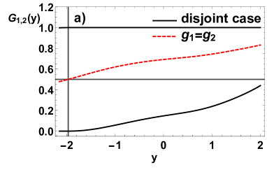
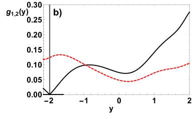
Figure 8: Solutions for the cumulative distribution functions of string end-points (a) and the corresponding probability distributions (b) in the $g_{1}=g_{2}$ and disjoint cases (dashed and solid lines, respectively). Model with 5 constituent partons per nucleon.

V Two-particle correlations

This section presents our model results for the two-particle correlations in pseudo-rapidity obtained for p-Pb and Pb-Pb collisions at $\sqrt{s_{\rm NN}}=5.02$ TeV. The findings presented here complement our earlier results Rohrmoser:2018shp for d-Au and Au-Au collisions at $\sqrt{s_{\rm NN}}=200$ GeV, with the main difference that at $\sqrt{s_{\rm NN}}=5.02$ TeV a wounded parton model with 4 or 5 constituents per nucleon is used, rather than the model with 3 constituents per nucleon applied at $\sqrt{s_{\rm NN}}=200$ GeV.

The interesting feature that at higher collision energies one needs in the wounded picture more partons per nucleon has also been discussed in Loizides:2016djv ; Bozek:2016kpf within analyses of the particle multiplicities $dN_{\rm ch}/d\eta$ in A-A collisions. Our results are in line with the conclusion of Loizides:2016djv , stating that whereas the fits at RHIC collision energies lead to 3 constituents partons, higher collision energies prefer about 5 partons per nucleon.

Two-particle correlations in $A$-$B$ collisions are defined as

$$C_{AB}(\eta_{1},\eta_{2})=\frac{\langle N(\eta_{1},\eta_{2})\rangle}{\langle N(\eta_{1})\rangle\langle N(\eta_{2})\rangle},$$ (9)

where $N(\eta_{1},\eta_{2})$ is the number of pairs with one particle in a bin centered at $\eta_{1}$ and the other in a bin centered at $\eta_{2}$, and $N(\eta_{i})$ is the number of particles in a bin centered at $\eta_{i}$. To the extent that $\eta\approx y$ (see the discussion in Sec. IV) and applying Eqs. (6,7), we may write

$$C_{AB}(\eta_{1},\eta_{2})\approx C_{AB}(y_{1},y_{2}),$$ (10)

since the Jacobian factors $d\eta/dy$ cancel out between the numerator and denominator.

In analogy to the profile for the emission of individual particles from a single string, a two-particle profile for the emission of particle pairs from single strings is Rohrmoser:2018shp

$$f_{2}(y_{1},y_{2}) = \omega^{2}G_{1}[{\rm min}(y_{1},y_{2})]\left\{1-G_{2}[{\rm max}(y_{1},y_{2})]\right\}$$ (11)

$$+ (1\leftrightarrow 2).$$

With this profile one obtains the correlation in pseudorapidity for particle pairs emitted from all strings in $A$-$B$ collisions as

$$C_{AB}(y_{1},y_{2})=1+\frac{{\rm cov}_{AB}(y_{1},y_{2})}{f(y_{1})f(y_{2})},$$ (12)

where ${\rm cov}_{\rm AB}(y_{1},y_{2})$ is

$${\rm cov}_{\rm AB} (y_{1},y_{2})=$$

$$\langle N_{A}\rangle{\rm cov}(y_{1},y_{2})+\langle N_{B}\rangle{\rm cov}(-y_{1},-y_{2})$$

$$+ {\rm var}(N_{A}){f(y_{1})}{f(y_{2})}+{\rm var}(N_{B}){f(-y_{1})}{f(-y_{2})}$$

$$+ {\rm cov}(N_{A},N_{B})\left[{f(y_{1})}{f(-y_{2})}+{f(-y_{1})}{f(y_{2})}\right].$$

Contributions to this expression come from emission of a hadron pair from the same string (associated to a wounded parton in $A$ or $B$ nucleus) and from the case where the two hadrons originate from different strings.

We emphasize that while the different string end-point distributions found in the previous section yield the same one-body emission spectra by construction, the same is not in general true for the corresponding two-particle correlations. Indeed, noticeable differences occur, as can be seen in Fig. 9, where results for $C_{\rm AB}(\eta_{1},\eta_{2})\simeq C_{\rm AB}(y_{1},y_{2})$ in both the $g_{1}=g_{2}$ and the disjoint cases are shown: Both cases yield correlations with a ridge-like structure along the $\eta_{1}=\eta_{2}$ direction. However for the $g_{1}=g_{2}$ case the ridge is higher than that of the disjoint case and, thus, exhibits a steeper decrease in the $\eta_{1}=-\eta_{2}$ direction. We found the same qualitative behavior also for correlations from d-Au and Au-Au collisions at $200$ GeV Rohrmoser:2018shp . For comparison, we also show in Fig. 9c) the results for the $4$ constituent model in the disjoint case, which is close to the $5$ constituent case from panel b).

To analyze $C_{\rm AB}(y_{1},y_{2})$ in more quantitative detail, we also study its projections on the Legendre polynomials Bzdak:2012tp

$$a_{nm} = \frac{\int_{-Y}^{Y}{dy_{1}}\int_{-Y}^{Y}{dy_{2}}C(y_{1},y_{2})T_{n}\left(\frac{y_{1}}{Y}\right)T_{m}\left(\frac{y_{2}}{Y}\right)}{\int_{-Y}^{Y}{dy_{1}}\int_{-Y}^{Y}{dy_{2}}C(y_{1},y_{2})}\,,$$ (14)

where we follow the choice of $Y=2.4$ of the ATLAS collaboration in order to be able to compare with their results. The dominant contributions to $C_{\rm AB}(y_{1},y_{2})$ are represented by the $a_{11}$ coefficients. Our model results for p-Pb and Pb-Pb collisions at $\sqrt{s_{\rm NN}}=5.02$ TeV are shown in Fig. 10 as a function of the number of charged particles $N_{\rm ch}$ that are produced within the collisions. As expected, the larger fall-off from the ridge for the correlations in the $g_{1}=g_{2}$ case is reflected in larger $a_{11}$ coefficients. Our results are shown in comparison to values extracted from ATLAS data for Pb-Pb collisions at $\sqrt{s_{NN}}=2.76$ TeV and p-Pb collisions at $\sqrt{s_{NN}}=5.02$ TeV from Aaboud:2016jnr . We use the data for $a_{11}$ subtracted by the contribution coming from the short range interactions.

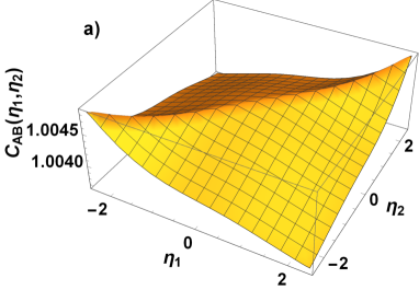
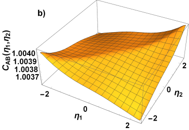
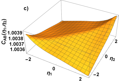
Figure 9: Correlations $C(\eta_{1},\eta_{2})$ in pseudorapidity for the $g_{1}=g_{2}$ (a) and the disjoint (b) cases for the $5\%$ most central Pb-Pb collisions at $\sqrt{s_{\rm NN}}=5.02$ TeV for the model with 5 constituent partons per nucleon. In (c) the disjoint case for the model with 4 constituent partons per nucleon is shown.

To show our model results as functions of $\langle N_{\rm ch}\rangle$ rather than $\langle N_{+}\rangle$, we infer from Eq. (2) that

$$\langle N_{\rm ch}\rangle=\langle N_{+}\rangle\int_{-Y}^{Y}d\eta f_{s}(\eta)\,.$$ (15)

From this relation we obtain the proportionality $\langle N_{\rm ch}\rangle=5.76\langle N_{+}\rangle$ and $\langle N_{\rm ch}\rangle=5.43\langle N_{+}\rangle$ in the case of p-Pb and Pb-Pb collisions, respectively (both with $5$ constituents per nucleon). For the $4$ constituent model the corresponding values are $\langle N_{\rm ch}\rangle=6.97\langle N_{+}\rangle$ and $\langle N_{\rm ch}\rangle=6.64\langle N_{+}\rangle$ for p-Pb and Pb-Pb collisions, respectively.

We note from Fig. 10 that the model results for the $a_{11}$ coefficient for the disjoint case are close to the ATLAS data, compared to the $g_{1}=g_{2}$ case which largely overestimates the data by about a factor of 4. We alert the reader that for the Pb-Pb there is a mismatch in the collision energy, as the model analysis is carried for $\sqrt{s_{NN}}=5.02$ TeV, while the data are available for $\sqrt{s_{NN}}=2.76$ TeV. Numerically, the mismatch is not significant. For comparison, we show in Fig. 10 the results for the $4$ and $5$ constituent model, which are very close to each other.

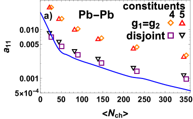
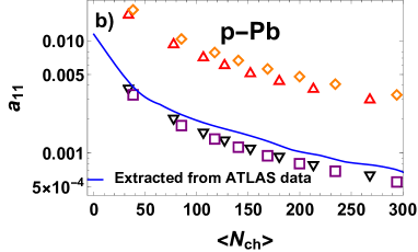
Figure 10: Model results for the coefficients $a_{\rm 11}$ for Pb-Pb (a) and p-Pb (b) collisions at $\sqrt{s_{\rm NN}}=5.02$ TeV, corresponding to the $g_{1}=g_{2}$ and disjoint cases, plotted as functions of the number of charged particles $N_{\rm ch}$ (points), in comparison to experimental data from ATLAS Aaboud:2016jnr (solid line) at $\sqrt{s_{NN}}=2.76$ TeV and at $\sqrt{s_{NN}}=5.02$ TeV for Pb-Pb and p-Pb collisions respectively. Models with 4 and 5 constituent partons per nucleon.

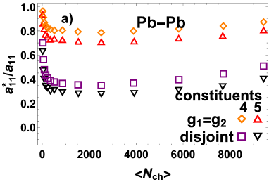
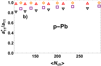
Figure 11: Ratios $a^{\ast}_{11}/a_{11}$ for Pb-Pb (a) and p-Pb (b) collisions at $\sqrt{s_{\rm NN}}=5.02$ TeV as functions of the number of charged particles $N_{\rm ch}$. Models with 4 and 5 constituent partons per nucleon.

We note that the model results for $a_{11}$ scale approximately as $1/N_{\rm ch}\sim 1/N_{+}$, as follows from Eqs. (12,V). Speaking of the decomposition (V), it is interesting to separate the $\langle N_{A}\rangle{\rm cov}(y_{1},y_{2})+\langle N_{B}\rangle{\rm cov}(-y_{1},-y_{2})$ term originating from intrinsic correlations of emission from a string, from the remainder coming from the fluctuation of the number of strings. Following Rohrmoser:2018shp , we denote the corresponding Legendre coefficient as $a_{11}^{\ast}$. Then the ratio $a_{11}^{\ast}/a_{11}$ is a measure of the intrinsic correlations compared to the total. This ratio is plotted in Fig. 11 for the models with 4 and 5 constituents as a function of the number of produced charged particles $N_{\rm ch}$, both p-Pb and Pb-Pb collisions. As can be seen, for the disjoint case which is close to the data, for the Pb-Pb the ratio is around 0.4, indicating a comparable share of the contributions from intrinsic string end-point fluctuations and the fluctuation of the number of strings. For the p-Pb case, the corresponding ratio is above 0.8, thus the intrinsic fluctuations dominate here.

VI p-p collisions

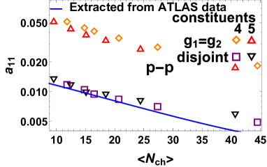
Figure 12: The Legendre coefficient $a_{\rm 11}$ for p-p collisions at $\sqrt{s_{\rm NN}}=5.02$ TeV, in comparison to the ATLAS data Aaboud:2016jnr at $\sqrt{s_{\rm NN}}=13$ TeV. Model with 4 and 5 constituent partons per nucleon.

With the nucleon substructure present in the model with several constituent partons, it is possible to carry out the correlation analysis also for the p-p collisions. In doing so, we use the same emission profile $f(\eta)$, obtained earlier from fitting the Pb-Pb and p-Pb pseudorapidity spectra at $\sqrt{s_{NN}}=5.02$ TeV. As before, the numbers of wounded partons are obtained with GLISSANDO 3 Bozek:2019wyr and the negative binomial distribution is overlaid according to Eq. (3). The results, compared to ATLAS data Aaboud:2016jnr at $\sqrt{s_{\rm NN}}=13$ TeV, are presented in Fig. 12. We note a fair agreement between the model and the experiment, again for the disjoint case. Again, the cases with 4 and 5 partons per nucleon are close to each other.

VII Summary and Conclusions

The basic conclusion of our study is that a very simple semi-analytic approach involving strings of fluctuating end-points is capable of explaining the basic features of the long-range two-particle correlation data in pseudorapidity, as measured by the ATLAS Collaboration Aaboud:2016jnr . In particular, the model with 4 or 5 constituent partons per nucleon and the disjoint distributions for the two fluctuating end-points reasonably describes the data for Pb-Pb, p-Pb, and p-p collisions. This explains why more sophisticated models incorporating the string breaking mechanism, such as used in various popular Monte Carlo generators, work in describing the longitudinal correlations.

Our approach merges the wounded constituent model with a generic description of string breaking that was first presented in Broniowski:2015oif and Rohrmoser:2018shp , and used for nuclear collisions at $\sqrt{s_{NN}}=200$ GeV at RHIC. The extension to the LHC energies, presented here for $\sqrt{s_{NN}}=5.02$ TeV, seems phenomenologically successful. Further tests of the model could be performed when the experimental correlation analysis at other collision energies, broader pseudorapidity coverage, and for other systems become available.

- (1) M. Rohrmoser and W. Broniowski, Phys. Rev. C99, 024904 (2019)
- (2) W. Broniowski and P. Bożek, Phys. Rev. C93, 064910 (2016)
- (3) B. Andersson, G. Gustafson, G. Ingelman, and T. Sjostrand, Phys. Rept. 97, 31 (1983)
- (4) X.-N. Wang and M. Gyulassy, Phys. Rev. D44, 3501 (1991)
- (5) Z.-W. Lin, C. M. Ko, B.-A. Li, B. Zhang, and S. Pal, Phys. Rev. C72, 064901 (2005)
- (6) T. Sjöstrand, S. Ask, J. R. Christiansen, R. Corke, N. Desai, P. Ilten, S. Mrenna, S. Prestel, C. O. Rasmussen, and P. Z. Skands, Comput. Phys. Commun. 191, 159 (2015)
- (7) C. Bierlich, G. Gustafson, L. Lönnblad, and H. Shah, JHEP 10, 134 (2018)
- (8) S. Ferreres-Solé and T. Sjöstrand, Eur. Phys. J. C78, 983 (2018)
- (9) A. Capella, U. Sukhatme, C.-I. Tan, and J. Tran Thanh Van, Phys. Rept. 236, 225 (1994)
- (10) K. Werner, I. Karpenko, T. Pierog, M. Bleicher, and K. Mikhailov, Phys. Rev. C82, 044904 (2010)
- (11) T. Pierog, I. Karpenko, J. Katzy, E. Yatsenko, and K. Werner(2013), arXiv:1306.0121 [hep-ph]
- (12) A. Białas, M. Błeszyński, and W. Czyż, Nucl. Phys. B111, 461 (1976)
- (13) R. J. Glauber in Lectures in Theoretical Physics, W. E. Brittin and L. G. Dunham eds., (Interscience, New York, 1959) Vol. 1, p. 315
- (14) W. Czyż and L. C. Maximon, Annals Phys. 52, 59 (1969)
- (15) A. Białas, W. Czyż, and W. Furmański, Acta Phys. Polon. B8, 585 (1977)
- (16) A. Białas, K. Fiałkowski, W. Słomiński, and M. Zieliński, Acta Phys. Polon. B8, 855 (1977)
- (17) A. Białas and W. Czyż, Acta Phys. Polon. B10, 831 (1979)
- (18) V. V. Anisovich, Yu. M. Shabelski, and V. M. Shekhter, Nucl. Phys. B133, 477 (1978)
- (19) S. Eremin and S. Voloshin, Phys. Rev. C67, 064905 (2003)
- (20) P. K. Netrakanti and B. Mohanty, Phys. Rev. C70, 027901 (2004)
- (21) A. Białas and A. Bzdak, Phys. Lett. B649, 263 (2007)
- (22) A. Białas and A. Bzdak, Phys. Rev. C77, 034908 (2008)
- (23) B. Alver, M. Baker, C. Loizides, and P. Steinberg(2008), arXiv:0805.4411 [nucl-ex]
- (24) G. Agakishiev et al. (STAR), Phys. Rev. C86, 014904 (2012)
- (25) S. S. Adler et al. (PHENIX), Phys. Rev. C89, 044905 (2014)
- (26) P. S. C. Loizides, J. Nagle, SoftwareX 1-2, 13 (2015)
- (27) A. Adare et al. (PHENIX), Phys. Rev. C93, 024901 (2016)
- (28) R. A. Lacey, P. Liu, N. Magdy, M. Csanád, B. Schweid, N. N. Ajitanand, J. Alexander, and R. Pak(2016), arXiv:1601.06001 [nucl-ex]
- (29) P. Bożek, W. Broniowski, and M. Rybczyński, Phys. Rev. C94, 014902 (2016)
- (30) L. Zheng and Z. Yin, Eur. Phys. J. A52, 45 (2016)
- (31) E. K. G. Sarkisyan, A. N. Mishra, R. Sahoo, and A. S. Sakharov, Phys. Rev. D94, 011501(R) (2016)
- (32) J. T. Mitchell, D. V. Perepelitsa, M. J. Tannenbaum, and P. W. Stankus, Phys. Rev. C93, 054910 (2016)
- (33) O. S. K. Chaturvedi, P. K. Srivastava, A. Kumar, and B. K. Singh, Eur. Phys. J. Plus 131, 438 (2016)
- (34) C. Loizides, Phys. Rev. C94, 024914 (2016)
- (35) M. J. Tannenbaum, Mod. Phys. Lett. A33, 1830001 (2017)
- (36) M. Barej, A. Bzdak, and P. Gutowski, Phys. Rev. C97, 034901 (2018)
- (37) M. Barej, A. Bzdak, and P. Gutowski(2019), arXiv:1904.01435 [hep-ph]
- (38) A. Białas and W. Czyż, Acta Phys. Polon. B36, 905 (2005)
- (39) P. Bożek, W. Broniowski, M. Rybczyński, and G. Stefanek, Comput. Phys. Commun. 245, 106850 (2019)
- (40) J. Adam et al. (ALICE), Phys. Lett. B772, 567 (2017)
- (41) G. Aad et al. (ATLAS), Eur. Phys. J. C76, 199 (2016)
- (42) B. B. Back et al. (PHOBOS), Phys. Rev. C65, 031901 (2002)
- (43) J. Adam et al. (ALICE), Phys. Rev. C91, 064905 (2015)
- (44) A. Bzdak and D. Teaney, Phys.Rev. C87, 024906 (2013)
- (45) M. Aaboud et al. (ATLAS), Phys. Rev. C95, 064914 (2017)