Learning Tests Traces

Abstract

Modern software projects include automated tests written to check the programs’ functionality. The set of functions invoked by a test is called the trace of the test, and the action of obtaining a trace is called tracing. There are many tracing tools since traces are useful for a variety of software engineering tasks such as test generation, fault localization, and test execution planning. A major drawback in using test traces is that obtaining them, i.e., tracing, can be costly in terms of computational resources and runtime. Prior work attempted to address this in various ways, e.g., by selectively tracing only some of the software components or compressing the trace on-the-fly. However, all these approaches still require building the project and executing the test in order to get its (partial, possibly compressed) trace. This is still very costly in many cases. In this work, we propose a method to predict the trace of each test without executing it, based only on static properties of the test and the tested program, as well as past experience on different tests. This prediction is done by applying supervised learning to learn the relation between various static features of test and function and the likelihood that one will include the other in its trace. Then, we show how to use the predicted traces in a recent automated troubleshooting paradigm called Learn, Diagnose, and Plan (LDP), instead of the actual, costly-to-obtain, test traces. In a preliminary evaluation on real-world open-source projects, we observe that our prediction quality is reasonable. In addition, using our trace predictions in LDP yields almost the same results comparing to when using real traces, while requiring less overhead.

I Introduction

The number of software projects and their size increase every day, while their time-to-market decreases. As a result, the number of bugs in software projects increase. Bugs damage the performance of software products and directly affect their customers. Therefore, software companies heavily invest in software quality and quality-related costs can consume as much as 60% of the development budget [1].

To maintain software quality, modern software projects include automated tests written to check the programs’ functionality. The set of functions invoked by a test is called the trace of the test. Many tools and research papers use test traces to perform a range of software engineering tasks, including test generation, bug isolation, and managing test execution. In test generation tools, traces are collected and used to compute coverage, which is the union of the sets of functions in the traces of the generated tests. Maximizing coverage is a standard objective in popular test generation frameworks, such as EvoSuite [2]. In bug isolation, traces are used by software diagnosis algorithms such as Barinel [3] to localize the root cause of observed bugs. Traces are also used to prioritize which tests to execute [4, 5].

A main drawback in using traces for all of the above tasks is that collecting traces is costly in terms of computational resources and runtime. This is because in order to obtain the trace of a test, one must build the project and execute the test while applying techniques such as byte-code manipulation to record its trace. All these activities can be very costly in real-sized projects, and the size of the resulting trace can be prohibitively large. Prior worked partially addressed this by compressing the trace while it is collected [6, 7] and by choosing selectively which software components to include in a trace [8, 9, 10, 11]. These approaches are very useful, but still require executing the test.

In this work, we propose to learn to predict the trace of a test without executing it. This prediction relies only on static properties of the test and the tested program, as well as previously collected traces of other tests. The first contribution of our work is to define the trace prediction problem and model it as Binary classification problem. Then, we propose to use a supervised learning algorithm over traces of previously executed tests to solve this classification problem, and suggest easy-to-extract features to do so. This is the second contribution of this work.

One of the benefits of having a trace prediction algorithm is that it can be used instead of real traces in software engineering tasks. We show this for the task of software troubleshooting. In particular, we propose to integrate our test prediction algorithm in a recently proposed automated troubleshooting paradigm called LDP [5]. LDP aims to identify the root cause of an observed bug, and does so by using a combination of techniques from the Artificial Intelligence (AI) literature. It uses a software diagnosis algorithm to output candidate diagnoses. If this set is too large, LDP uses a test planning (TP) algorithm to choose which tests to perform next in order to collect more information for the diagnosis algorithm. Prior work on the TP component of LDP assumed that the test planner knows the traces of the test it is planning to execute. We propose a simple TP algorithm that can use the predicted traces instead of the actual, costly-to-obtain, test traces. This is the third contribution of this work.

Finally, we perform a small-scale evaluation of our trace prediction algorithm and our TP algorithm in LDP on real-world open-source projects. Results show that while prediction quality can be improved, it is sufficiently accurate to be used by our TP algorithm to guide LDP to troubleshoot bugs almost well as when using real traces.

II Background and Problem Definition

An automated test is a method that executes a program in order to check if it is working properly. The outcome of running a test is either that the test has passed or failed, where a failed test indicates that the program is not behaving properly. The trace of a test is the set of software components, e.g., classes or methods, that were activated during the execution of a test. We denote by $\textit{outcome}(t)$ and $\textit{trace}(t)$ the outcome and trace, respectively, of a test $t$.

Modern software programs include a large set of automated tests. For a given program of interest, we denote its set of automated tests by T, and its set of software components by COMPS. Note that for every test $t\in\textit{T}$ it holds that $\textit{trace}(t)\subseteq\textit{COMPS}$.

There are several techniques for obtaining the trace of test after executing it. A common way to obtain the trace of a test $t$ is to modify the program’s source code so that it records every function invocation, and then run $t$. For example, in Java programs such code modification can be done in runtime using byte-code manipulation frameworks such as ASM (http://asm.objectweb.org), BCEL (http://jakarta.apache.org/bcel), and SERP (http://serp.sourceforge.net). Another way to obtain the trace of a test is to execute it with a debugging tool, and, again, record every function invocation. These tracing techniques have been used in practice in various tracing tools, such as iDNA [12] and Clover (https://www.atlassian.com/software/clover). For a survey of tracing tools, see [13].

All these tools require running the test in order to obtain its trace. However, running a test can costly in terms of computational resources and time. Moreover, tracing techniques usually incur non-negligible overhead, e.g., for printing out the trace to a file. The goal of this research is to output the trace of an automated test $t$ without actually running it. We call this problem the trace prediction problem, and apply supervised learning to solve it.

III Learning to Predict a Trace

In this section, we provide relevant background in supervised learning and show how the trace prediction problem can be solved with supervised learning techniques.

III-A Supervised Learning

Supervised learning is perhaps the most widely used branch of Machine Learning (ML). Broadly speaking, supervised learning aims to learn from example input–output pairs a function that maps from input to output [14]. Supervised learning is commonly used to solve classification tasks. A classification task is the task of mapping a label to a given instance, where the set of possible labels is discrete and finite. A binary classification task is a classification task in which there are only two possible labels.

To solve a classification task using supervised learning, one needs to accept as input a set of instance-label pairs, i.e., a set of instances and their label. This is called a training set. Supervised learning algorithms work, in general, as follows: they extract features from every instance in the training set, and then run an optimization algorithm to search for parameters of a chosen mathematical model that maps values of these features to the correct label.

The output of a supervised learning algorithm is this mathematical model along with optimized values for its parameter. In the context of classification, this is called a classifier. A classifier can be used to output a label for a previously unseen instance, by extracting the features of this instance, inserting their values to the learned mathematical model, and outputting the resulting label.

III-B Trace Prediction as a Binary Classification Problem

Trace prediction can be viewed as a binary classification task. An instance in trace prediction is a pair $(t,c)$ where $t$ is a test and $c$ is a software component. The label is true if and only if $c$ is in the trace of $t$, i.e., iff $c\in\textit{trace}(t)$. The corresponding binary classifier is a classifier that accepts a pair $(t,c)$ where $t\in\textit{T}$ and $c\in\textit{COMPS}$, and outputs true if $c\in\textit{trace}(t)$ and false otherwise. We refer to such a classifier as a trace classifier. A trace classifier can be used to solve the trace prediction problem: for a given test $t$, run over all software components $c\in\textit{COMPS}$, and return only the components labeled as true by the classifier.

To solve this binary classification problem with supervised learning, we need a training set of test-component pairs and their correct label. To generate such a training set, we propose to run a subset $T_{train}\subset\textit{T}$ of all automated tests and record their trace. Generating this training set is costly. However, as we show in our experimental results only a small fraction of all tests is needed in order to obtain a sufficiently large training set. In addition, this training step can be done only once for every major software version, as opposed to every time one needs to obtain a trace of a test.

Given a training set, we can use an off-the-shelf supervised learning algorithm to learn a trace classifier. Key factors in the successful application of such algorithms are (1) which optimization algorithm to use, (2) which classifier model to choose, and (3) which features to extract from each instance. There are many general-purpose optimization algorithms for supervised learning, such as stochastic gradient descent [15] and Adam [16]. Similarly, popular classifier models such as decision trees [17] and forests [18], support vectors [19], and artificial neural networks [20], are commonly used in supervised learning. Designing useful features, however, is often done manually, with the aid of a domain expert.

III-C Feature for Trace Prediction

We extracted two types of features for trace prediction: features based on call graph analysis and features based on syntactic similarity.

III-C1 Features based on Call Graph Analysis

Running a test and extracting its trace is a form of dynamic code analysis. Static code analysis is an alternative common form of computer program analysis in which the program’s source code is analyzed without running the actual program. Thus, information extracted in this way is especially suitable for our purposes, since we aim to predict a test’s trace without running it.

Static code analysis tools output a variety of source code artifacts, such as code smells [21] and code complexity metrics. Call graph is a standard output of many static code analysis tools that is particularly useful for our purposes. It is a graph in which every node represents a function and there is a directed edge from $n$ to $n^{\prime}$ if the function represented by $n$ contains a call the function represented by $n^{\prime}$. Note that it does not mean that every invocation of $n$ will also invoke $n^{\prime}$, e.g., when the call to $n^{\prime}$ is in an “if” branch that was not reached.

Obviously, the call graph contains important information with respect to whether a function is in the trace of a test or not. For example, if there is a path in the call graph from a function $n$ to a different function $n^{\prime}$, then there exists an invocation of $n$ in which $n^{\prime}$ will be in its trace. In practice, for a given project, we generate its static call graph and extract the following features for a given test function $t\in\textit{T}$ and $c\in\textit{COMPS}$:

• Path existence. A Boolean feature that indicates whether there is a path between $t$ and $c$.

• Shortest path. The length of the shortest path between $t$ and $c$.

• Target in-degree. The in-degree of $c$.

• Source out-degree. The out-degree of $t$.

III-C2 Syntactic Similarity

A major limitation of call graphs generated by static code analysis is that they cannot detect dynamic function calls. These are function calls that occur e.g., due to function polymorphism or dynamically loaded libraries. Thus, a component $c$ may be in a trace of a test $t$ even if there is no path from $t$ to $c$ in the call graph. More generally, the call graph by itself does not provide sufficient information to determine the trace of a test.

To partially fill this gap, we consider another type of features that is based on syntactic similarity between the name of the test $t$ and the name of the component $c$. The underlying intuition is that if a test and a class have similar names, then it increases the chances that the $t$ aims to use $c$ and thus it will be in its trace.

Based on this intuition, we extracted the following features:

• Common words. The number of words that appear in both the test’s name and in the component’s name. Names were split to words using Camel notation, i.e., a capital letter is assumed to mark the start of a new word. This notation is standard in Java and other languages.

• Name distance. The edit distance between the test’s name and the component’s name, normalized to the [0,1] range by dividing the edit distance with the length of the longer name.

In our experiments, every test $t$ is a method in a JUnit test class $T$ and every component $c$ is a method in some class $C$. We computed the above syntactic similarity features for the names of $t$ and $c$, and for the names of $T$ and $C$. Thus, we extracted four syntactic similarity features: class common words, method common words, class name distance, and method name distance.

IV Troubleshooting with Predicted Traces

In this section, we present how our trace prediction algorithm can be used for automated software troubleshooting. In particular, we show how our trace prediction algorithm can be integrated in LDP [5], a newly-proposed Artificial Intelligence (AI)-based paradigm for software troubleshooting. For completeness, we first provide relevant background on software troubleshooting and LDP.

IV-A The Learn, Diagnose, and Plan (LDP) Paradigm

Software troubleshooting is a process that starts with an undesirable behavior of a given software, and ends by isolating the software components that should be fixed to avoid this undesirable behavior. Concretely, we focus on the case where one or more automated tests fail, and aim to find the software components that should be fixed to make all tests pass.

LDP is a paradigm for software troubleshooting that contains three AI components: a learning algorithm, a diagnosis algorithm, and a planning algorithm.

IV-A1 Learning to predict bugs

This LDP component is fundamentally a software fault prediction algorithm [22]. It automatically matches between previously reported bugs and the code revisions made to fix them to create a dataset of buggy software components. This dataset is used to train a classifier that accepts a software component and outputs whether that component is expected to have a bug or not. Such learning-based software fault prediction algorithms work surprisingly well, at least for mature programs [23, 24]. In addition, most learning-based software fault prediction algorithms can output a real value that represents the confidence that a component is faulty.

IV-A2 Diagnosing software bugs

This LDP component is a software diagnosis algorithm. A software diagnosis algorithm, also known as software fault localization, accepts a set of executed tests and their outcomes, and outputs one or more diagnoses. Each diagnosis is a set of software components that may have caused the observed bug. There are many approaches for software diagnosis, for a survey see [25]. The LDP diagnosis component is based on Barinel [3], a state-of-the-art software diagnosis algorithm. Barinel follows a spectrum-based fault localization (SFL) approach. It accepts as input a set of tests that were executed, the outcomes of these tests, and their traces. Then, it runs a fast hitting-set algorithm to find minimal sets of components that “hit” the trace of every failed test. Every such set is returned as a diagnosis.

Barinel can scale to real-world software systems and has many extensions [26, 27]. However, it tends to output a large set of diagnoses, denoted $\Omega$. While each of these diagnoses is a set of components that may have caused the bug, only one diagnosis is correct, i.e., contain the actual components that caused the bug. Thus, returning a large set of diagnoses is not useful. To mitigate this, Barinel outputs for every diagnosis $\omega\in\Omega$ also a score, denoted $p(\omega)$, that roughly correspond to the likelihood that the components in $\omega$ are indeed the root cause of the failed tests. In LDP, this score function is modified so that it is affected by the fault likelihood estimates from LDP’s learning component [5]. Nevertheless, in many cases too many diagnoses are still returned that have similar, non-negligible, scores.

IV-A3 Planning additional tests

This LDP component is a planning algorithm. The input to this planning algorithm is (1) the set of tests that were not executed to so far and $T_{left}\subset\textit{T}$ (2) the set of diagnoses $\Omega$ that was returned by the diagnosis algorithm (DA), along with their scores. Its output is the next test to execute.

In LDP, the selected test is executed, obtaining its trace and outcome. This information is added to the set of tests given to DA, which outputs a potentially more refined set of diagnoses. If this set is still too large to be useful, the TP algorithm chooses an additional test to be executed. This process continues until either the correct diagnoses has been found, or all tests in T have been executed (i.e., $T_{left}=\emptyset$), or the time allowed for automated troubleshooting has expired.

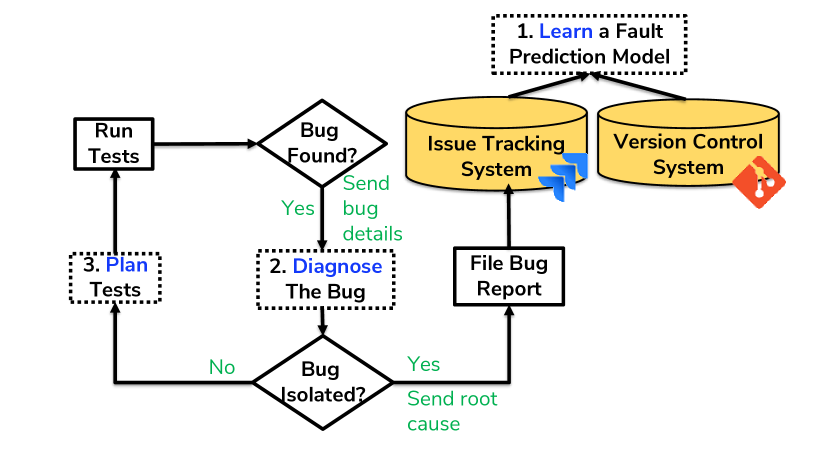
Figure 1: An illustration of the LDP paradigm. Dashed rectangles are the AI components.

Figure 1 illustrates the LDP workflow. In the background, the learning component (dashed rectangle 1) learns a fault prediction model by extracting information about bugs that were previously reported in the issue tracker (JIRA) and their fix was committed in the version control system (Git). Then, when a test fails, the diagnose component (dashed rectangle 2) runs a DA and outputs a set of diagnoses. If needed, the planning component chooses which text to execute next (dashed rectangle 3).

IV-B Test Planning with Predicted Traces

Several TP algorithms have been proposed for troubleshooting [4, 5], including sophisticated algorithms that compute information gain of each tests, or aim to solve an exponentially large Markov Decision Problem (MDP). These algorithms are computationally expensive, and, importantly, require knowing the trace of every test in $T_{left}$ although it has not been executed.

This is, of course, not realistic in practice. One approach to address this is to store the traces of every executed test. This has several limitations. First, it requires storing large amounts of data. Second, it requires running all tests at least once while recording their trace. This is very time consuming. Third, the trace of a test may change after modifying some component, and thus stored traces may be outdated and incorrect.

We propose a novel TP algorithm that uses a trace prediction algorithm instead of knowing the actual trace of every test. This TP algorithm requires a trace classifier, which we assume is generated using the trace prediction algorithm described in Section III. In addition, we require that the trace classifier output a confidence score that roughly approximates the likelihood that the classifier is correct. As mentioned earlier, most learning-based classifier can output such a value. In our case, an instance is a component-test pair $(c,t)$ and the label is true iff $c\in\textit{trace}(t)$. Thus, the confidence of a trace classifier approximates the likelihood that $c$ really is is in $\textit{trace}(t)$. We denote this confidence score by $\textit{conf}(c,t)$.

Our TP algorithm also relies on computing the health state [28] of every component $c\in\textit{COMPS}$ for the set of diagnoses and their scores returned by the DA. The health state of $c$, denoted $H(c)$, is defined as the sum of the scores of every diagnosis $\omega\in\Omega$ in which $c$ is assumed faulty. Formally,

$$H(c)=\sum_{\omega\in\Omega|c\in\omega}p(\omega)$$ (1)

If the score of a diagnosis is indeed its probability to be correct and $\Omega$ is the set of all diagnoses, then $H(c)$ is the probability that $c$ is faulty [28].

Finally, we are ready to define our TP algorithm. It computes for every test $t$ the following utility function $U(t)$:

$$U(t)=\sum_{c\in\textit{COMPS}}\textit{conf}(c,t)\cdot H(c)$$ (2)

This utility function aims to approximate the expected number of faulty components in $\textit{trace}(t)$. Our TP algorithm returns the test with the highest utility. For practical reasons, in our implementation we computed the utility of a trace $t$ by only summing only the term $\textit{conf}(c,t)\cdot H(c)$ for the 40 components that are most likely in $\textit{trace}(t)$ according to our trace classifier.

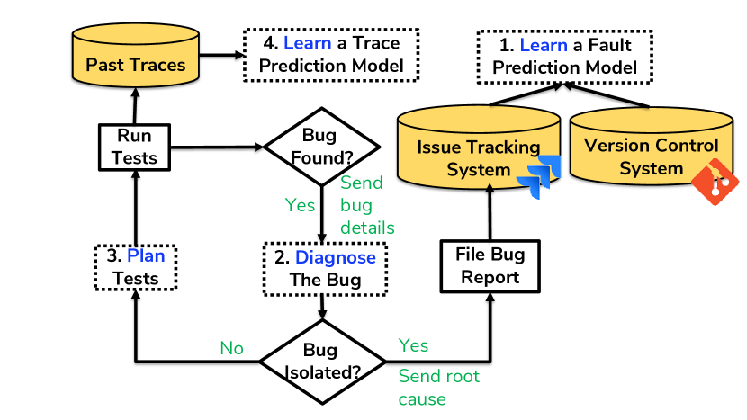
Figure 2: An illustration of the LDP paradigm with our trace prediction added to the learning component. Dashed rectangles are the AI components.

Figure 2 shows how our trace prediction integrates well in LDP. Whenever a test is executed and its trace is collected, this is added to the training set used to train our trace classifier (dashed rectangle 4). The TP algorithm (dashed rectangle 3) can then use it as described above.

V Experimental Results

In the first part of this section, we evaluate experimentally the performance of our trace prediction algorithm (Section III). In the second part of this section, we evaluate experimentally the performance of our TP algorithm, which uses trace prediction, in the context of software troubleshooting (Section IV).

TABLE I: General statistics for the projects used in our experiments.

Project	Lang	Math
First release	2002	2004
Last release	2018	2018
Average number of functions	4,000	7,400
Average number of tests	1,660	3,500
Test average length	11	39

For our experiments, we used two popular open source projects: Apache Commons Math and Apache Commons Lang. Both projects are Java projects and use the Git version control system. Table I lists general details about these projects, including the date of the first and last release, the average number of functions and tests in a version, and the average length of a trace of a test.

V-A Trace Prediction Experiments

For each project, we chose a set of versions. For each version, we created a dataset of labeled component-test pairs by executing all available automated tests and collecting their traces. To speedup this process, we limited our tracing to 10% of the methods. Thus, for a version with 100 tests and 2,000 methods, we obtained a dataset with 20,000 instances. This dataset was split equally (50/50) to train and test sets.

V-A1 Learning algorithms

For learning, we used a feed-forward artificial neural network and trained it using back-propagation. There are many possible neural network architectures, solvers, and activation functions. The configuration we used is a single hidden layer with 30 neurons, the Adam optimization algorithm [16], the ReLu activation function [29], and a maximum of 3,000 iterations for training. We also tried other configurations, including different optimization algorithms (Newton’s method and stochastic gradient descent) and activation function (Sigmoid), but the above configuration worked best. In addition, we tried a deep neural network architecture that includes 5 hidden layers, each with 30 neurons. We refer to the first architecture as “NN” and to the deep 5-layers architecture as “DNN”.

V-A2 Evaluation metrics

We used standard supervised learning metrics to evaluate our trace prediction algorithm. Specifically, we report the following metrics.

• True negatives (TN). Percentage of instances where the target function is not in the trace and it is classified correct as such.

• False positives (FP). Percentage of instances where the target function is not in the trace but it is incorrectly classified as in the trace.

• False negatives (FN). Percentage of instances where the target function is in the trace but it is incorrectly classified wrong as not in the trace.

• True Positives (TP). Percentage of instances where the target function is in the trace and it is classified correctly as such.

• Area under the receiver operating characteristic curve (AUC). The receiver operating characteristic (ROC) curve plots the TP rate against the FP rate for different threshold values. A perfect classifier has an AUC value of 1 and a random classifier has an AUC of 0.5.

• Acc. Accuracy is the ratio of instances that are classified correctly. This ratio is given by $\frac{TP+TN}{TP+TN+FP+NF}$.

All of these are standard machine learning metrics, commonly used to evaluate binary classifiers. For a more comprehensive discussion on these metrics, see [30].

TABLE II: Results of the prediction experiments.

Algorithm	Project	AUC	Acc	TN	FP	FN	TP
NN	Lang	0.795	0.998	99.68%	0.07%	0.10%	0.15%
DNN	Lang	0.779	0.998	99.69%	0.04%	0.12%	0.15%
NN	Math	0.602	0.993	99.28%	0.27%	0.35%	0.10%
DNN	Math	0.596	0.996	99.52%	0.03%	0.36%	0.09%

V-A3 Results

Table II presents the results of our prediction experiments. Note that the results in every data cell is the average obtained by our algorithm over all datasets.

The accuracy obtained for both architectures (NN and DNN) is very high. For example, in the Math project the average accuracy is 0.993 and 0.996 for NN and DNN, respectively. However, these high accuracy results are misleading, because our dataset is highly imbalanced. That is, most methods are not part of a given trace, and thus the true label of most instances (i.e., most method-test pairs) is negative. For example, according to Table I there are 4000 functions in Lang and the average number of functions called in a test is 11. Thus, less than 0.3% of all instances are expected to be positives. This means that a naive trace classifier that says for every pair ($c,t$) that $c$ is not in the trace of $t$, which be quite accurate.

AUC is a common metric to evaluate binary classifiers over imbalanced datasets. Indeed, we observe that the AUC for NN and DNN is far from perfect. For example, in the Lang project, the AUC of NN and DNN is 0.795 and 0.779, respectively, while the AUC of NN and DNN is only 0.602 and 0.596, respectively. We hypothesize that it is possible to increase the AUC by incorporating known techniques for handling imbalanced datasets, such as under-sampling and over-sampling [31], as well as devising more sophisticated features. However, as we show in the next set of experiments, our trace prediction was accurate enough to guide software troubleshooting effectively.

TABLE III: Feature importance in the Lang project.

Feature name	NN	DNN
Shortest path	0.10	0.16
Target in-degree	0.02	0.00
Path existence	0.12	0.00
Method common words	0.00	0.02
Method names distance	0.04	0.00

To gain a better understanding of the impact of the different features (detailed in Section III-C), we performed an all but one analysis. An all but one analysis works as follows. We choose a feature $f$ and train two models: one with all features and one with all features except $f$. Then, we evaluate the performance of both models on the test set. The importance of $f$ is computed by the difference between the AUC of the model that considers all features and the AUC of the model that considers all features except $f$. Table III shows the importance of each feature using this analysis, for the NN and DNN models. As can be seen, the most important features are those that are based on static code analysis, namely, the length of the path in the call graph from the test to the method (“Path length”) and whether such a path exists (“Path existence”). The features based on syntactic similarity – common words and name distance – are also useful, but to a lesser degree.

Interestingly, we do not observe a significant difference between the shallow neural network (NN) and the deep one (DNN). For example, the AUC of NN and DNN in the Lang is 0.795 and 0.779, respectively. Therefore, for the rest of our experiments, we used the NN. Note that the design space of constructing a DNN is very large and one may come up with a DNN architecture that would be more efficient.

V-B Troubleshooting Experiment

In the next set of experiments, we evaluated how our trace prediction can be used in LDP, as described in Section IV.

V-B1 TP algorithms

We compared our TP algorithm, referred to as Predicted, to two baselines. The first uses the real traces of the available tests. That is, it assumes that $\textit{conf}(c,t)$ is one iff $c\in\textit{trace}(t)$ and zero otherwise. We refer to this is Oracle. The second baseline TP algorithm we used, referred to as Random, chooses a test randomly. Note that Oracle cannot be used in practice, since we cannot check if $c$ is in $\textit{trace}(t)$ without executing it. Thus, Oracle serves as an “upper bound” to the performance of our TP algorithm, while Random is expected to be worse than our TP algorithm, serving as a “lower bound”.

V-B2 Evaluation metrics

To compare between these test planning methods, we run LDP as described in Section IV on a set of previously reported bugs from the Lang and Math projects. These bugs were collected from the Defects4j repository [32] and by mining the issue tracking and version control systems of these projects. In total, we used 112 bugs for Lang and 48 bugs for Math.

For each of these reported bugs we conducted the following experiment. First, we chose a set of initial tests and verified that at least one of them is marked as a failed test. A test is marked as a failed test if its trace contains the buggy function. Then, we run LDP using one of the evaluated TP algorithms until one of the following conditions occur:

• A diagnosis was found whose likelihood is above $S$, where $S$ is a parameter referred to as the score threshold. We set $S=0.7$ in our experiments.

• More than $B$ tests have been run, where $B$ is a parameter, referred to as the test budget. We set $B=50,75,100,125,$ and $150$ in our experiments.

If the troubleshooting process has stopped because of the first condition, we say it has converged. Otherwise, we say that it has timed out. Converging is desirable because it means the troubleshooting process believes it has successfully isolated the root cause of the bug.

For each bug, we performed three experiments, one for each TP algorithm. In each experiment, we recorded the number of tests performed until the troubleshooting process either converged or timed out. We refer to this as the number of steps performed. Fewer steps is better, as it means less testing effort for troubleshooting.

For out TP algorithm, we used a trace classifier that was trained on an earlier version of the code. That is, when running an experiment on a bug reported for version $X$, we trained the trace prediction model on the dataset extracted for version $X-1$ or earlier. Also, recall that only 10% of all methods were used to train the trace classifier.

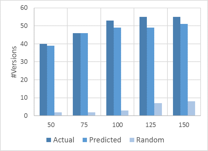
Figure 3: Lang project. # of versions that converged for different test budgets.

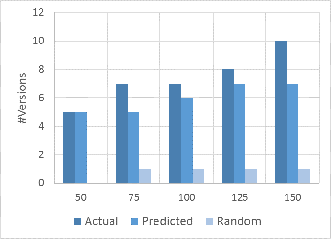
Figure 4: Math project. # of versions that converged for different test budgets.

V-B3 Results

Figures 3 and 4 plots the number of bugs in which each algorithm has converged, for $B=50,75,100,125$, and $150$, for the Lang and Math projects, respectively. The results clearly show that Random fails to converge much more often, compared to Predicted and Oracle. For example, in the Lang project with a test budget of 150, Random converges in fewer than 10 versions while both Oracle and Predicted converged in more than 50 versions.

When comparing Prediction and Oracle, we observe very similar results in most cases, with a small advantage for Oracle. The advantage of Oracle is expected because it uses the actual test traces to choose which test to execute. However, this advantage is very small, suggesting that our trace prediction algorithm works well for guiding tests in a software troubleshooting process.

Note that the advantage of Oracle over Predicted is larger for Math than for Lang. This corresponds to the trace prediction accuracy results reported in the previous section, as the AUC for Lang is significantly higher than the AUC for Math. This shows the relation between the strength of the trace prediction and the effectiveness of the troubleshooting.

To gain a deeper insight into our results, Figures 5 and 6 presents the number of steps until each algorithm converged for the cases where it did not reach a timeout. The $y$ axis represents the number of steps performed, for different versions and TP algorithms. Every line represents a different TP algorithm and every data point represents a single experiment, i.e., the number of steps until convergence for a specific bug and TP algorithm. The data points for every test planning algorithms are sorted on the $x$-axis according to their number of steps. Of course, being lower on the $y$-axis is better, as it shows fewer steps are need to coverage. In this figure, we did not show bugs for which all algorithms reached the budget without converging.

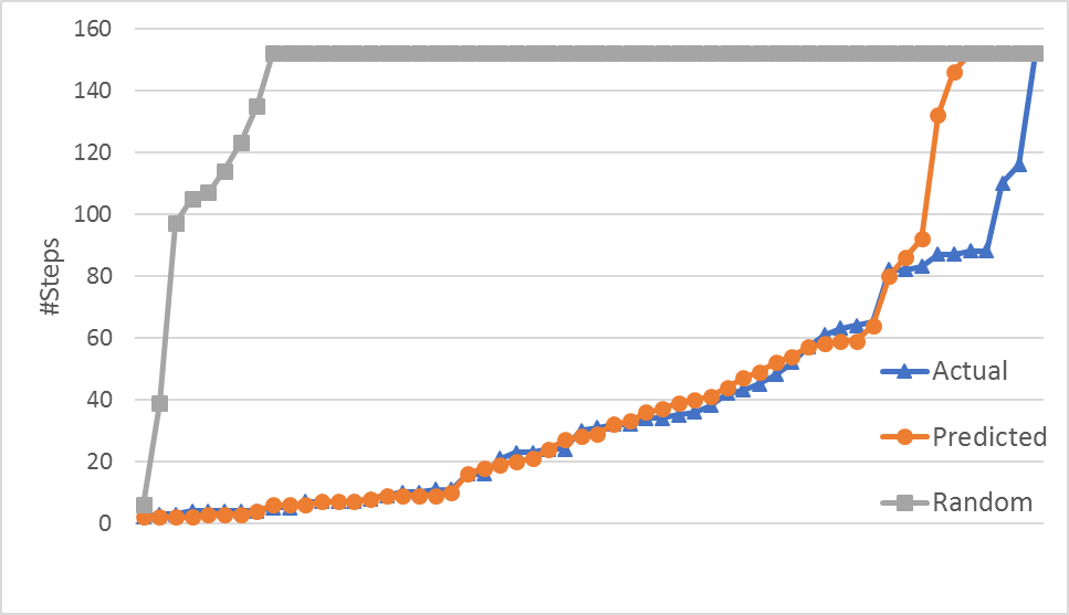
Figure 5: Lang project. # of steps until reached one of the stopping conditions.

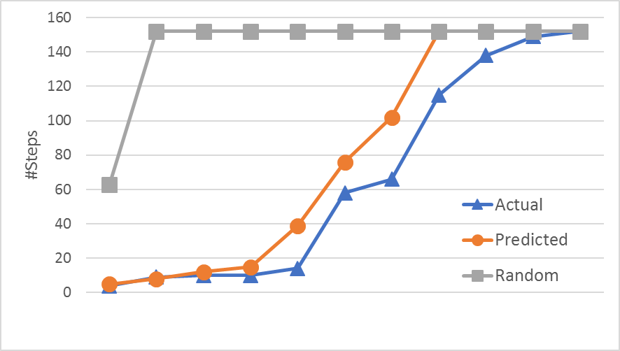
Figure 6: Math project. # of steps until reached one of the stopping conditions.

Similar trends are observed in these results. Random performs significant worst than Predicted and Oracle, in both projects. Again, Oracle performs the same or better than Prediction in almost all cases. However, the results clearly show that the difference between them is not large.

VI Related Work

Tracing the dynamic execution of a program has many applications, and consequently, a large body of research is devoted to study different aspects of efficient and effective tracing. To the best of our knowledge, no prior work attempted to learn how to predict a trace of a test by analyzing traces of other tests. The most similar research we have found is Daniel and Boshernitsan [33] work on predicting the effectiveness of test generation algorithms. They propose to use supervised learning to train a classifier that predicts the coverage of a given function obtained by running a given test. The label they aimed to predict is how much the function is covered, while we aim to predict the actual trace. Thus, our trace prediction can be used to estimate coverage, but not vice versa. An interesting future work would be to use our trace prediction algorithm to estimate coverage.

One branch of research studied different ways to visualize collected traces in a meaningful way [34, 35]. A different branch aims to reduce the size of the generated traces, e.g., by compressing them on-the-fly [6, 7] or by identifying the parts of the code that are not relevant for the task at hand and thus can be removed from the trace (or not traced to begin with) [8]

Other prior work aimed to minimize the cost of tracing by choosing intelligently which components to monitor, consider this as a sensor-placement problem [11]. Liblit et al. [9, 10] proposed a statistical method to sample traces, in the context of bug isolation. Their approach is somewhat similar to our work, but in their task they are given a part of the trace. Thus, they must execute the test while our trace prediction algorithm does not.

VI-A Threats to Validity and Limitations

Our approach for trace prediction requires a large set of automated tests to be available and executable in past versions of the code. Thus, our work is not suitable for projects in an early stage. Future work may study how to learn trace prediction from one project to the other. The main limitation of this research is the breadth of our experimental evaluation. Future work will perform a large-scale study over more projects and more programming languages.

VII Conclusion and Future Work

We proposed a trace prediction algorithm that learns from a small fraction of existing traces how to predict whether a given software component is in a trace of a given test. Our approach is based on modeling the trace prediction problem as a binary classification problem and applying supervised learning to solve it. To this end, we propose features based on call graph analysis and syntactic similarity, and show experimentally that they work well on two open-source projects. Then, we show how predicted traces can be used in a TP algorithm, as part of LDP, a recently proposed software troubleshooting paradigm. We evaluate LDP without TP algorithm, showing that it converges much faster than random test selection, and almost the same as an Oracle TP algorithm, that knows a-priori the tests’ traces.

While our results are encouraging, there is much to do in future work. First, the quality of our trace prediction is far from perfect. This is because the available data is highly imbalanced, where the vast majority of component-test pairs are negative (i.e, the component is not in the trace of the test). Future work can attempt to address this using known techniques for imbalanced dataset. In addition, future work will extend our experimental evaluation to more projects, and include a user case study. Another interesting direction is to combine our trace prediction algorithm with symbolic execution methods, as well as strongly TP algorithms.

VIII Acknowledgements

This research was partially funded by the Israeli Science Foundation (ISF) grant #210/17 to Roni Stern.

References

- [1] A. Engel and M. Last, “Modeling software testing costs and risks using fuzzy logic paradigm,” Journal of Systems and Software, vol. 80, no. 6, pp. 817–835, 2007.
- [2] G. Fraser and A. Arcuri, “Evosuite: automatic test suite generation for object-oriented software,” in European conference on Foundations of software engineering, 2011, pp. 416–419.
- [3] R. Abreu, P. Zoeteweij, and A. J. C. van Gemund, “Spectrum-based multiple fault localization,” in Automated Software Engineering (ASE). IEEE, 2009, pp. 88–99.
- [4] T. Zamir, R. T. Stern, and M. Kalech, “Using model-based diagnosis to improve software testing,” in AAAI Conference on Artificial Intelligence, 2014.
- [5] A. Elmishali, R. Stern, and M. Kalech, “An artificial intelligence paradigm for troubleshooting software bugs,” Engineering Applications of Artificial Intelligence, vol. 69, pp. 147–156, 2018.
- [6] S. P. Reiss and M. Renieris, “Encoding program executions,” in International Conference on Software Engineering (ICSE). IEEE, 2001, pp. 221–230.
- [7] S. Taheri, S. Devale, G. Gopalakrishnan, and M. Burtscher, “ParLoT: Efficient whole-program call tracing for hpc applications,” in Programming and Performance Visualization Tools. Springer, 2017, pp. 162–184.
- [8] S. Tallam, C. Tian, R. Gupta, and X. Zhang, “Enabling tracing of long-running multithreaded programs via dynamic execution reduction,” in International Symposium on Software Testing and Analysis, ser. ISSTA. ACM, 2007, pp. 207–218.
- [9] B. Liblit, A. Aiken, A. X. Zheng, and M. I. Jordan, “Bug isolation via remote program sampling,” in ACM SIGPLAN conference on Programming Language Design and Implementation (PLDI), vol. 38, no. 5, 2003, pp. 141–154.
- [10] B. Liblit, M. Naik, A. X. Zheng, A. Aiken, and M. I. Jordan, “Scalable statistical bug isolation,” in ACM SIGPLAN conference on Programming Language Design and Implementation (PLDI), vol. 40, no. 6, 2005, pp. 15–26.
- [11] X. Zhao, K. Rodrigues, Y. Luo, M. Stumm, D. Yuan, and Y. Zhou, “Log20: Fully automated optimal placement of log printing statements under specified overhead threshold,” in Symposium on Operating Systems Principles. ACM, 2017, pp. 565–581.
- [12] S. Bhansali, W.-K. Chen, S. De Jong, A. Edwards, R. Murray, M. Drinić, D. Mihočka, and J. Chau, “Framework for instruction-level tracing and analysis of program executions,” in International Conference on Virtual Execution Environments. ACM, 2006, pp. 154–163.
- [13] K. Alemerien and K. Magel, “Examining the effectiveness of testing coverage tools: An empirical study,” International journal of Software Engineering and its Applications, vol. 8, no. 5, pp. 139–162, 2014.
- [14] S. J. Russell and P. Norvig, Artificial intelligence: a modern approach. Pearson, 2016.
- [15] L. Bottou, “Stochastic gradient learning in neural networks,” Proceedings of Neuro-Nımes, vol. 91, no. 8, p. 12, 1991.
- [16] D. P. Kingma and J. L. Ba, “Adam: A method for stochastic optimization,” in International Conference for Learning Representations (ICLR), 2015.
- [17] J. R. Quinlan, “Induction of decision trees,” Machine learning, vol. 1, no. 1, pp. 81–106, 1986.
- [18] L. Breiman, “Random forests,” Machine learning, vol. 45, no. 1, pp. 5–32, 2001.
- [19] C.-C. Chang and C.-J. Lin, “Libsvm: A library for support vector machines,” ACM transactions on intelligent systems and technology (TIST), vol. 2, no. 3, p. 27, 2011.
- [20] S. S. Haykin, Neural networks and learning machines. Pearson, 2009, vol. 3.
- [21] E. Van Emden and L. Moonen, “Java quality assurance by detecting code smells,” in Conference on Reverse Engineering. IEEE, 2002, pp. 97–106.
- [22] C. Catal, “Software fault prediction: A literature review and current trends,” Expert systems with applications, vol. 38, no. 4, pp. 4626–4636, 2011.
- [23] R. Malhotra, “A systematic review of machine learning techniques for software fault prediction,” Applied Soft Computing, vol. 27, pp. 504–518, 2015.
- [24] M. K. Amir Elmishali, Roni Stern, “DeBGUer: A tool for bug prediction and diagnosis,” in Conference on Innovative Applications of Artificial Intelligence (IAAI), 2019.
- [25] W. E. Wong, R. Gao, Y. Li, R. Abreu, and F. Wotawa, “A survey on software fault localization,” Transactions on Software Engineering, 2016.
- [26] A. Elmishali, R. Stern, and M. Kalech, “Data-augmented software diagnosis,” in AAAI Conference on Artificial Intelligence, 2016, pp. 4003–4009.
- [27] A. Perez and R. Abreu, “Leveraging qualitative reasoning to improve sfl,” in IJCAI, 2018, pp. 1935–1941.
- [28] R. Stern, M. Kalech, S. Rogov, and A. Feldman, “How many diagnoses do we need?” in AAAI Conference on Artificial Intelligence, 2015, pp. 1618–1624.
- [29] V. Nair and G. E. Hinton, “Rectified linear units improve restricted boltzmann machines,” in International Conference on Machine Learning (ICML), 2010, pp. 807–814.
- [30] T. Mitchell, Machine learning. McGraw Hill, 1997.
- [31] N. V. Chawla, K. W. Bowyer, L. O. Hall, and W. P. Kegelmeyer, “SMOTE: synthetic minority over-sampling technique,” Journal of artificial intelligence research, vol. 16, pp. 321–357, 2002.
- [32] R. Just, D. Jalali, and M. D. Ernst, “Defects4J: A database of existing faults to enable controlled testing studies for java programs,” in International Symposium on Software Testing and Analysis, 2014, pp. 437–440.
- [33] B. Daniel and M. Boshernitsan, “Predicting effectiveness of automatic testing tools,” IEEE/ACM International Conference on Automated Software Engineering (ICSE), pp. 363–366, 2008.
- [34] W. De Pauw, E. Jensen, N. Mitchell, G. Sevitsky, J. Vlissides, and J. Yang, “Visualizing the execution of java programs,” in Software Visualization. Springer, 2002, pp. 151–162.
- [35] B. Cornelissen, D. Holten, A. Zaidman, L. Moonen, J. J. Van Wijk, and A. Van Deursen, “Understanding execution traces using massive sequence and circular bundle views,” in International Conference on Program Comprehension (ICPC). IEEE, 2007, pp. 49–58.