TESTING NONPARAMETRIC SHAPE RESTRICTIONS

Abstract.

We describe and examine a test for a general class of shape constraints, such as constraints on the signs of derivatives, U-(S-)shape, symmetry, quasi-convexity, log-convexity, $r$-convexity, among others, in a nonparametric framework using partial sums empirical processes. We show that, after a suitable transformation, its asymptotic distribution is a functional of the standard Brownian motion, so that critical values are available. However, due to the possible poor approximation of the asymptotic critical values to the finite sample ones, we also describe a valid bootstrap algorithm.

1. INTRODUCTION

Hypothesis testing is one of the most relevant tasks in empirical work. Such tests include situations when the null and alternative hypothesis are assumed to belong to a parametric family of models. In a second type of tests, known as diagnostic or lack-of-fit tests, only the null hypothesis is assumed to belong to a parametric family leaving the alternative nonparametric. The latter type of testing has a distinguished and long literature starting with the work of Kolmogorov, see Stephens [83], for testing the probability distribution function and in a time series context by Grenander and Rosenblatt [44] for testing the white noise hypothesis. In a regression model context a new avenue of work started in Stute [84], and Andrews [5] with a more econometric emphasis, using partial sums empirical methodology, see also Stute et al. [86] or Koul and Stute [59], among others. The methodology has attracted a lot of attention and it rivals tests based on a direct comparison between a parametric and a nonparametric fit to the regression model as first examined in Härdle and Mammen [51] or Hong and White [55]. One advantage of tests based on partial sums empirical methodology, when compared to the approach in [51], is that the former does not require the choice of a bandwidth parameter for its implementation, see also Nikabadze and Stute [75] for some additional advantages. However, a possible drawback is that the asymptotic distribution depends, among other possible features, on the estimator of the parameters of the model under the null hypothesis in a nontrivial way, as it was shown in Durbin [33], and hence its implementation requires either bootstrap algorithms, see Stute et al. [85], or the so-called Khmaladze’s [57] martingale transformation, see also earlier work and ideas in Brown at al. [12].

In this paper, though, we are interested in a third type of testing where neither the null hypothesis nor the alternative has a specific parametric form. This type of hypothesis testing can be denoted as testing for qualitative or shape restrictions. Many shape properties (including monotonicity, convexity/concavity, strong convexity, log-convexity) are widespread in economics and other disciplines. It is also often of interest to analyse statistical and economic relationships that do not have a persistent shape pattern on the whole domain but rather switch the patterns in the domain (for example, U-shaped or S-shaped relations).

To fix ideas, consider the nonparametric regression model

(1.1) $$y_{i} =m\left(x_{i}\right)+u_{i}\text{,}$$

$$E[u_{i}|x_{i}] =0,$$

where $x$ has bounded support $\mathcal{X=}:\left[\underline{x},\overline{x}\right]$ and $m\left(\cdot\right)$ is smooth. More specific conditions on the sequences $\left\{u_{i}\right\}_{i\in\mathbb{Z}}$ and $\left\{x_{i}\right\}_{i\in\mathbb{Z}}$ will be given in Condition $C1$ in Section 2.2. Our main aim is testing whether the regression function $m\left(x\right)$ possesses shape properties captured by a general null hypothesis

(1.2) $$H_{0}:\text{ \ }m\in\mathcal{M}_{0},$$

where the class of interest $\mathcal{M}_{0}$ is a subset of smooth functions from $\mathcal{X}$ to $\mathbb{R}$. Our requirement on the class $\mathcal{M}_{0}$ is given in Condition $C0$ below, which is formulated in a way to directly relate it to the methodology we employ later to approximate and estimate $m(\cdot)$.

Before we introduce Condition $C0$, let us introduce some useful notations. Let $\mathcal{B}_{q,L}$ denote the set of all B-splines of degree $q$ with knots that split $\mathcal{X}$ into $L^{\prime}$ equally spaced intervals. A generic element in this set is written as a linear combination $m_{\mathcal{B}}(x)\equiv\sum_{\ell=1}^{L}\beta_{\ell}p_{\ell,L}\left(x\right)$, where $L=L^{\prime}+q$, and $\left\{p_{\ell,L}\left(\cdot\right)\right\}$ is the collection of the B-splines base for the chosen system of knots (more details will be given in Section 2.1). Any element in $\mathcal{B}_{q,L}$ can be fully characterised by the vector $(\beta_{1},\ldots,\beta_{L})\in\mathbb{R}^{L}$ and constraints on this vector can be mapped into constraints on the B-spline. For any set $S_{q,L}\subseteq\mathbb{R}^{L}$ we can, thus, define

$$\mathcal{M}_{s_{q,L}}=:\left\{m_{B}(\cdot)\in\mathcal{B}_{q,L}\;|\;(\beta_{1},\ldots,\beta_{L})\in S_{q,L}\right\}.$$

Condition C0. There is a set $S_{q,L}\subseteq\mathbb{R}^{L}$ for any $L^{\prime}$ (and, hence, for any $L=L^{\prime}+q$) that satisfies the following properties:

• $S_{q,L}$ does not depend on data $\left\{x_{i}\right\}_{i\in\mathbb{Z}}$ and, thus, is non-stochastic;

• the boundary of $S_{q,L}$ consists of a finite number of smooth surfaces;

• (1.3) $$\mathcal{H}\left(\mathcal{M}_{0},\mathcal{M}_{S_{q,L}}\right)\rightarrow 0\quad\text{as}\quad L\rightarrow\infty\text{,}$$

  where $\mathcal{H}$ is the Hausdorff distance in the supremum norm in the space of continuous functions from $\mathcal{X}$ to $\mathbb{R}$.

Condition $C0$ essentially states that the membership in $\mathcal{M}_{0}$ can be captured by restrictions on parameters $\{\beta_{\ell}\}_{\ell=1}^{L}$ which become necessary and sufficient restrictions as the system of knots becomes increasingly dense in $\mathcal{X}$. In addition, these restrictions on $\{\beta_{\ell}\}_{\ell=1}^{L}$ do not depend on the available data, which adds to the attractiveness of our approach for implementation purposes.

Our idea will be to test the null hypothesis

(1.4) $$H_{0}^{B}:\text{ \ }(\beta_{1},\ldots,\beta_{L})\in S_{q,L}$$

formulated in terms of the approximation for $m(\cdot)$. As may be expected, our methodology readily extends to situations when the domain $\mathcal{X}$ is partitioned into several intervals with different null hypotheses in the spirit of (1.2) formulated on different intervals in the partitioning. An illustration of this situation is given in Example 2 below.

We shall now illustrate several examples of shape classes $\mathcal{M}_{0}$ that satisfy condition $C0$. In Section 2.1, after a more thorough discussion of B-splines we indicate the corresponding sets $S_{q,L}$ for each of these examples. As we shall discuss in Section 2.1, the first two examples pertain to the case where in the constraints on the coefficients of the B-splines approximation are linear, whereas in the last two examples these constraints are nonlinear. It is important to note that these examples are an illustration of the scope of our approach rather than a full list of properties that our methodology could test.

Example 1 (Constraints, may hold simultaneously, on the derivatives of $m\left(\cdot\right)$).

(1.5) $$H_{0}:d_{r}\cdot m^{\left(r\right)}\left(x\right)\geq c_{r}\text{,}~{}\ \ \ \ r\in R\text{,}$$

where $R$ is a finite subset of $\mathbb{N}^{+}$, $d_{r}\in\left\{-1,1\right\}$ and $c_{r}$ are known constants.

In this hypothesis, we specify conditions on inequalities for several derivatives simultaneously. If $c_{r}=0$, then we have familiar restrictions on the sign of the $r$-th derivative. Special cases in this example include testing for monotonicity ($r=1$ and $c_{1}=0$), testing for convexity/concavity ($r=2$ and $c_{2}=0$), testing for strong $\lambda$-convexity ($r=2$ and $c_{2}=\lambda>0$), testing for monotonicity and concavity simultaneously, etc.

The properties of monotonicity, convexity/concavity or the ones in terms of higher-order derivatives are so commonplace in economics and other disciplines that the applications are too many to list. For instance, a demand function is expected to be a decreasing function of the price of a good, whereas a supply function is expected to be increasing. In single-object auctions, the equilibria analyzed commonly are those in which buyers play monotone strategy functions and mark-ups are often monotone functions of the bids (see e.g. [60]). In other economic relationships it is often of importance whether the marginal returns are increasing or decreasing, which naturally amounts to convexity and concavity, respectively.

Note that in the context of isotone/monotone regressions the literature goes back to Brunk [13] and Wright [91], and in the context of convex regressions to Hildreth [54]. A more detailed coverage of this literature is given in Section 2.

As mentioned above, our methodology can be used when different properties can be conjectured on different intervals of the partition $\mathcal{X}$. This is illustrated in the next example.

Example 2 (changing shape patterns on the domain; symmetry; quasi-convexity).

In this case, we can take a partitioning of $\mathcal{X}$ at points $\tau_{0}=\underline{x}<\tau_{1}<\ldots<\tau_{J-1}<\tau_{J}=\overline{x}$, and formulate the null hypothesis on the signs of various derivatives on the intervals in this partitioning. The null hypothesis in this case would be

(1.6) $$H_{0} :d_{r_{j}}\cdot m^{\left(r_{j}\right)}\left(x\right)\geq 0,\quad x\in\left(\tau_{j},\tau_{j+1}\right],$$

$$\text{ for some fixed }r_{j}\in\mathbb{N},\quad j=0,\ldots,J-1\text{,}$$

$d_{r_{j}}\in\left\{-1,1\right\}$. The partitioning points $\tau_{j}$ either have to be known or have to be consistently estimated at a suitable rate before the testing procedure.

This type of hypotheses include, among others, the important scenarios of $U$-shape, $S$-shape. For example, U-shape is the property of a function first decreasing and then increasing. So, we write the null hypothesis of U-shape with the switch at $s_{0}$ as

(1.7) $$H_{0}:\text{ \ }\left\{\begin{array}[]{c}m\left(x^{1}\right)>m\left(x^{2}\right)\quad\text{ when }\quad x^{1}<x^{2}\leq s_{0}\\ m\left(x^{1}\right)>m\left(x^{2}\right)\quad\text{ when }\quad x^{1}>x^{2}\geq s_{0}.\end{array}\right.$$

The issues associated with testing properties outlined in this example relate to how functional pieces from different partition intervals are connected to each other. We can incorporate various scenarios – e.g., we can require that different pieces are joint continuously, or smoothly at all or some partition points.

It goes without saying that we can consider several different partitions and test simultaneously properties formulated on various intervals of these partitions. For example, one could consider a function defined on $[0,1]$ and conjecture that $m(\cdot)$ is convex on $(0,s_{0}$, concave on $(s_{0},1]$, decreasing on $(0,0.3s_{0}]$, increasing on $(0.3s_{0},0.5s_{0}+0.5]$, and decreasing on $(0.5s_{0},1]$.

Examples of U-shaped relationships in economics and other disciplines can be found e.g. in [14], [22], [43], [45]. [87], [90], and in the discussions in [58], [65] and [82]. Inverse U-shaped relationships include the case of the so-called single-peaked preferences, which is an important class of preferences in psychology and economics. Examples of S-shaped relationships between unexpected earnings and stock price in accounting can be found in [24] or [39], among others. S-shaped growth curves of the adopted population in a large society is a generally accepted empirical feature of innovation diffusion (see discussions in [80] or [88]). Thus, testing for an S-shape in this case would allow one to conclude whether technology evolves as one would expect.

Another shape property in this class of shape-changing patterns are the properties of quasi-convexity and quasi-concavity. Formally, the class $\mathcal{M}_{0}$ in (1.2) of quasi-convex functions is defined as

$$\mathcal{M}_{0}=\bigg{\{}\phi(\cdot):\;\forall\,x_{1},x_{2}\in\mathcal{X}\;\;\forall\lambda\in[0,1]\;\;\phi(\lambda x_{1}+(1-\lambda)x_{2})\leq\max{\big{\{}}\phi(x_{1}),\phi(x_{2}){\big{\}}}\bigg{\}}.$$

Since function $\phi$ is quasi-concave if and only if $-\phi$ is quasi-convex, we can easily write a description of the class of quasi-concave functions. A smooth function is quasi-convex if and only if it first decreases up to some point and then increases (giving a special case of monotonicity when such a switch point is located at one of the boundary points of the interval). Since this switch point may not be known a priori, it would have to be estimated. A further discussion of this is given later in Section 2.1.

The concept of quasi-convexity/quasi-concavity is quite important in economics and other disciplines. For example, it is known that indirect utility functions are quasi-convex provided that the direct utility function is continuous. Thus strict quasi-concavity (and continuity) of the production function provides a sufficient condition for the differentiability of the cost function with respect to input prices.

Finally, we mention another property related to this framework, which is the symmetry of a function around some point $s_{0}$. Without a loss of generality, we can take $s_{0}$ to be the center of the domain $[\underline{x},\overline{x}]$ and write the class of symmetric functions as

$$\mathcal{M}_{0}=\left\{\phi(\cdot):\;\forall\,x\in[\underline{x},s_{0}]\quad\phi(s_{0}-x)=\phi(s_{0}+x)\right\}.$$

Example 3 ($r$-convexity; $\rho$-convexity).

The null hypothesis of $\mathbf{r}$-convexity, $r\neq 0$, is described by the following $\mathcal{M}_{0}$;

$$\mathcal{M}_{0}=\bigg{\{}\phi(\cdot):\;\phi(\cdot)\geq 0,\quad\forall\,x_{1},x_{2}\in\mathcal{X}\quad\forall\lambda\in[0,1]\\ \phi(\lambda x_{1}+(1-\lambda)x_{2})\leq\log\left(\lambda e^{r\phi(x_{1})}+(1-\lambda)e^{r\phi(x_{2})}\right)^{\frac{1}{r}}\bigg{\}},$$

and for $r=0$ this property is described by

$$\mathcal{M}_{0}=\bigg{\{}\phi(\cdot):\;\phi(\cdot)\geq 0,\quad\forall\,x_{1},x_{2}\in\mathcal{X}\quad\forall\lambda\in[0,1]\\ \phi(\lambda x_{1}+(1-\lambda)x_{2})\leq\lambda\phi(x_{1})+(1-\lambda)\phi(x_{2})\bigg{\}}.$$

The definition of $\mathbf{r}$-concave functions would reverse the inequalities. If we consider functions that are twice continuously differentiable, then the class of $r$-convex functions can be described as (see e.g. Avriel [6])

$$\mathcal{M}_{0}=\bigg{\{}\phi(\cdot):\;\phi(\cdot)\geq 0,\quad\forall\,x\in\mathcal{X}\quad r\left(\phi^{\prime}(x)\right)^{2}+\phi^{{\prime\prime}}(x)\geq 0\bigg{\}}.$$

A concept closely related to $r$-convexity/concavity is what is known as $\mathbf{\rho}$-convexity/concavity in the economics literature. Following [15], we can define the class of $\rho$-convex functions as follows: for $\rho\neq 0$,

$$\mathcal{M}_{0}=\bigg{\{}\phi(\cdot):\;\phi(\cdot)>0,\quad\forall\,x_{1},x_{2}\in\mathcal{X}\quad\forall\lambda\in[0,1]\\ \phi(\lambda x_{1}+(1-\lambda)x_{2})\leq\left(\lambda\phi(x_{1})^{\rho}+(1-\lambda)\phi(x_{2})^{\rho}\right)^{\frac{1}{\rho}}\bigg{\}},$$

and for $\rho=0$,

$$\mathcal{M}_{0}=\bigg{\{}\phi(\cdot):\;\phi(\cdot)>0,\quad\forall\,x_{1},x_{2}\in\mathcal{X}\quad\forall\lambda\in[0,1]\\ \phi(\lambda x_{1}+(1-\lambda)x_{2})\leq\phi(x_{1})^{\lambda}\phi(x_{2})^{1-\lambda}\bigg{\}}.$$

The definition of $\mathbf{\rho}$-concave functions would reverse the inequalities. It is obvious that for any $r=\rho$, a real-valued function $\phi$ is $r$-convex if and only if $e^{\phi}$ is $\rho$-convex.

It is also clear that $\rho$-convexity gives the standard definition of convexity when $\rho=1$ and gives log convexity for $\rho=0$.

In economics, $\rho$-concavity has been used to measure the curvature of demand functions, production functions, and distributions (i.e., density and distribution functions) of individual characteristics. It has also been employed in the areas of imperfect competition, auctions and mechanism design and public economics. Log-convexity and log-concavity are of particular interest in economics.

Our final example illustrates further shape properties well developed in the mathematical literature. This example first requires defining a mean function.

Definition 1 (mean function; Niculescu [74]).

A function $N:\mathbb{R}^{+}\times\mathbb{R}^{+}\rightarrow\mathbb{R}^{+}$ is called a mean function if

• $N(x_{1},x_{2})=N(x_{2},x_{1})$

• $N(x,x)=x$

• $x_{1}<N(x_{1},x_{2})<x_{2}$ whenever $x_{1}<x_{2}$

• $N(ax_{1},ax_{2})=aN(x_{1},x_{2})$ for all $a>0$

Examples of mean functions include the arithmetic mean (A), the geometric mean (G), the harmonic mean (H), the logarithmic mean and the identric mean.

Example 4 ($MN$-convexity).

For any two mean functions $M$ and $N$, the class of $\mathbf{MN}$-convex is defined as

$$\mathcal{M}_{0}=\bigg{\{}\phi(\cdot):\;\phi(\cdot)>0,\quad\forall\,x_{1},x_{2}\in\mathcal{X}\quad\phi(M(x_{1},x_{2}))\leq N(\phi(x_{1}),\phi(x_{2}))\bigg{\}}.$$

The definition of $\mathbf{MN}$-concavity would reverse the inequalities.

When we have different combinations of arithmetic (A), geometric (G) and harmonic (H) means, we end up with the following special cases of ${MN}$-convex functions (see e.g. [3]):

1. $m$ is AG-convex if and only if $\frac{m^{\prime}(x)}{m(x)}$ is increasing

2. $m$ is AH-convex if and only if $\frac{m^{\prime}(x)}{m^{2}(x)}$ is increasing

3. $m$ is GA-convex if and only if $xm^{\prime}(x)$ is increasing

4. $m$ is GG-convex if and only if $\frac{xm^{\prime}(x)}{m(x)}$ is increasing

5. $m$ is GH-convex if and only if $\frac{xm^{\prime}(x)}{m^{2}(x)}$ is increasing

6. $m$ is HA-convex if and only if $x^{2}m^{\prime}(x)$ is increasing

7. $m$ is HG-convex if and only if $\frac{x^{2}m^{\prime}(x)}{m(x)}$ is increasing

8. $m$ is HH-convex if and only if $\frac{x^{2}m^{\prime}(x)}{m^{2}(x)}$ is increasing.

We want to emphasize again that the examples given in this introduction are meant to illustrate the scope of applicability of our testing methodology rather than give an exhaustive list of potential application.

1.1. LITERATURE REVIEW ON TESTING FOR SHAPES

There is a range of the literature related to testing for monotonicity or convexity such as [11], Hall and Heckman [48], Ghosal et al. [42], Juditsky and Nemirovski [56], Wang and Meyer [89], Chetverikov [20], Schlee [81], Diack and Thomas-Agnan [29], Dumbgen and Spokoiny [32], Abrevaya and Jiang [1], Baraud et al. [7], Dette et al. [27].

Some of the work referenced above (such as [7], [32], [56]) focuses on the regression function in the ideal Gaussian white noise model, while our framework does not require such assumptions. In the aforementioned literature some papers, such as [7], [29] or [48], allow the explanatory variable to take only deterministic values. [1], [20] and [42] treat the explanatory variable as random but either require its full stochastic independence with the unobserved regression error ([20], [42]) or require the distribution of the error to be symmetric conditional on the explanatory variable, see [1], whereas we require a weaker mean independence of error condition. Some of the above-mentioned papers, such as [11], [48] or [89], do not give any asymptotic theory. Many of the approaches are tailored to a specific type of shape and their extensions to more general shape properties do not appear straightforward, if at all possible. Moreover, these tests are often targeted to detecting specific deviations from the null hypothesis. The violations of the null hypothesis, however, can come from different sources. A parametric test for U-shapes was suggested in [65], whereas [58] proposes a non-parametric test based on critical bandwidth giving sufficient conditions for its consistency. To the best of our knowledge, there is no formal approach in the literature to testing S-shapes or general shape properties formulated on intervals in a partitioning.

Also, to the best of our knowledge, this paper is the first to give a unified framework and a nonparametric methodology for testing (possibly simultaneously) a wide range of shape/qualitative constraints. Even for shape properties described in terms of the signs of the derivatives of the function, this methodology will, in particular, overcome some of the problems discussed above. But, of course, we want to make it clear that its applicability goes beyond such properties.

To be more specific, we propose a test based on a transformation, introduced in Khmaladze [57], of the partial sums empirical process similar to that in Stute [84]. Some of the properties of the test is that it converges to a standard Brownian motion, so that critical values of standard functionals such as Kolmogorov-Smirnov, Cramér -von-Mises or Anderson-Darling are readily obtained. As a consequence, our testing procedure has the same asymptotic distribution regardless of the shape constraints under consideration.

Another feature of our testing procedure is its flexibility as it is able to test simultaneously for more than one shape constraint – for instance, one could test monotonicity and log-convexity simultaneously. Finally, the test is easy to implement as it requires no more than “recursive” least squares.

The remainder of the paper is organized as follows. Section 2 introduces and motivates our nonparametric estimator of $m\left(x\right)$ and it compares the methodology against rival nonparametric estimators. It also describes the form that the sets $S_{q,L}$ in Condition $C0$ take for the examples given in the introduction. In Section 3, we describe the test and examine its statistical properties. Because the Monte-Carlo experiment suggests that the asymptotic critical values are not a good approximation of the finite sample ones, Section 4 introduces a bootstrap algorithm. Section 5 presents a Monte-Carlo experiment and some empirical examples, whereas Section 6 concludes with a summary and possible extensions of the methodology. The proofs are confined to the Appendix A which employs a series of lemmas given in Appendix B.

2. METHODOLOGY AND REGULARITY CONDITIONS

Before we present the procedure for testing the hypothesis given in (1.2), we introduce and motivate the type of nonparametric estimator that we shall use to estimate the regression function $m\left(x\right)$ under $H_{0}$ and/or $H_{1}$.

When testing for the null hypothesis of either monotonicity or convexity, several nonparameteric estimators have been considered in the literature. As mentioned in the introduction, early work on isotone/monotone regressions is Brunk [13] and Wright [91]. Friedman and Tibshirani [40] combines local averaging and isotonic regression, Mukerjee [71] and Mammen [66] propose a two-step approach, which involves smoothing the data by using kernel regression estimators in the first step, and then deals with the isotonization of the estimator by projecting it into the space of all isotonic functions in the second step. Hall and Huang [49] proposes an alternative method based on tilting estimation which preserves the optimal properties of the kernel regression estimator. Finally, a different approach to isotonization is based on rearrangement methods using a probability integral transformation, see Dette et al. [28] or Chernozhukov et al. [19]. When the null hypothesis is that of convexity, Hildreth [54] approach is based on estimating $m\left(\cdot\right)$ by least squares approach. Consistency, rate of convergence properties and pointwise convergence results for this estimator are established, respectively, in [50], [67] and [46]. The global behaviour of such an estimator is examined in [47]. Birke and Dette [9] examine an estimator based on first obtaining unconstrained estimate of the derivative of the regression function which is isotonized and then integrated.

Our main aim is to propose a testing methodology which is not only applicable for a wide range of shape properties but also able to perform valid statistical inferences. The narrowness of the above mentioned techniques would make it extremely difficult to make them work in our more general context. Besides, the implementation of these techniques is not always trivial and/or they often lack any asymptotic theory useful for the purpose of inference.

A different approach might be based on series estimation using polynomial and, in particular, Bernstein polynomials basis, see the survey by Chen [17], for results on sieve estimation in both nonparametric and semiparametric models. One motivation for the Bernstein polynomials is due to a well-known result that any continuous function can be approximated in the sup-norm by a Bernstein polynomial whose coefficients are the values of the function at uniform knot points. This property makes them an appealing candidate estimation method in our context. However, base Bernstein polynomials have an undesirable property of being highly correlated, making them difficult for our purposes – in particular, to obtain a valid Khmaladze’s transformation, which plays a key role in our results. This is discussed in more detail in Section 2.1.

Due to many of the aforementioned reasons, in this paper we shall employ B-splines and/or penalized B-splines known as P-splines. Our testing will rely on the ability to write our null hypothesis in terms of the coefficients of the B-spline approximation, leading us to utilizing Condition $C0$ and testing (1.4). Note that monotone regression splines (closely related to B-splines) were introduced by Ramsay [79] and later extended by Meyer [69] to estimate convex/concave function or functions that are, e.g., both monotone and convex. A distinct feature in our approach is, first, that we now take the use of B-splines to a different level of generality and, second, that we derive the asymptotic theory as the number of knots goes to infinity, and, third, that we allow the number of constraints on the coefficients of B-splines to increase with the number of knots. Both [79] and [69] consider the number of knots, and hence the number of constraints, to be fixed.

2.1. B-SPLINES (or P-SPLINES)

B-splines or P-splines are constructed from polynomial pieces joined at some specific points denoted knots. Their computation is obtained recursively, see [25], for any degree of the polynomial. It is well understood that the choice of the number of knots determines the trade-off between overfitting when there are too many knots, and underfitting when there are too few knots. The main difference between B-splines and P-splines is that the latter tend to employ a large number of knots but to avoid oversmoothing they incorporate a penalty function based on the second difference of the coefficients of adjacent B-splines, in contrast to the second derivative employed in [76], [77], see [36] for details.

The methodology and applications of constrained B-splines and P-splines are discussed by many authors, too many to review here. For more detailed discussions, see, among others, the monographs [25] and [31] for B-splines and [36], [10] for P-splines. Some literature on shape-preserving splines (for ordinary shapes such as monotonicity, convexity, etc.) includes, among others, [64], [68], [69] and [79].

In general, the B-spline basis of degree $q$

• takes positive values on the domain spanned by $q+2$ adjacent knots, and is zero otherwise;

• consists of $q+1$ polynomial pieces each of degree $q$, and the polynomial pieces join at $q$ inner knots;

• at the joining points, the $q-1$th derivatives are continuous;

• except at the boundaries, it overlaps with $2q$ polynomials pieces of its neighbours;

• at a given $x$, only $q+1$ B-splines are nonzero.

Assume that one is interested in approximating the regression function $m\left(x\right)$ in the interval $\left[\underline{x},\overline{x}\right]$. Then we split the interval $\left[\underline{x},\overline{x}\right]$ into $L^{\prime}$ equal length subintervals with $L^{\prime}+1$ knots, where each subinterval will be covered with $q+1$ B-splines of degree $q$. The total number of knots needed will be $L^{\prime}+2q+1$ (each boundary point $\underline{x}$, $\overline{x}$ is a knot of multiplicity $q+1$) and the number of B-splines is $L=L^{\prime}+q$. Thus, $m\left(x\right)$ is approximated by a linear combination of B-splines of degree $q$ with coefficients $(\beta_{1},\ldots,\beta_{L})$ as

(2.1) $$m_{\mathcal{B}}\left(x;L\right)=\sum_{\ell=1}^{L}\beta_{\ell}p_{\ell,L}\left(x;q\right)\text{,}$$

and where henceforth we shall denote the knots as $\{z^{k}\}$, $k=1,\ldots,L^{\prime}+2q+1$, where $\underline{x}=z^{1}=\ldots=z^{q+1}$ and $\overline{x}=z^{L^{\prime}+q+1}=\ldots=z^{L^{\prime}+2q+1}$.

B-splines share some properties which turns out to be very useful for our purpose. Indeed,

$$\left(a\right)~{}\sum_{\ell=1}^{L}p_{\ell,L}\left(x;q\right) = 1\text{ \ \ for all }x\text{ \ and }q\text{.}$$

$$\left(b\right)\text{ }\frac{\partial}{\partial x}m_{\mathcal{B}}\left(x;L\right) = :m_{\mathcal{B}}^{\prime}\left(x;L\right)=q\sum_{\ell=1}^{L-1}\frac{\triangle\beta_{\ell+1}}{z^{l+1+q}-z^{l+1}}p_{\ell+1,L}\left(x;q-1\right),$$

where $\triangle\beta_{\ell}=\beta_{\ell}-\beta_{\ell-1}$. In particular, $\left(a\right)$ indicates that B-splines, as is the case with Bernstein polynomials, are a partition of $1$. The property (b) states that the derivative of a B-spline of degree $q$ becomes a B-spline of degree $q-1$. Using this expression for the derivative and taking into account that the knot system effectively changes with the first and the last knots now removed (thus, the multiplicity of $\underline{x}$ and $\overline{x}$ becomes $q$ rather than $q+1$), one can derive an expression for the second derivative, and so on.

We now describe the structure that the sets $S_{q,L}$ take in the Examples 1-4 given in the previous section. One general idea, especially useful when dealing with shape constraints in Examples 3-4, for constructing $S_{q,L}$ is to enforce the shape property of interest at the chosen knots (for simplicity we can take equidistant ones). As $L\rightarrow\infty$, the knot system becomes dense in $\mathcal{X}$ and, thus, the shape property of interest becomes satisfied on an increasingly dense system of points in $\mathcal{X}$.

Example 1 (Cont.). For our general null hypothesis in (1.5), the set $S_{q,L}$ is given by

$$S_{q,L}=\bigg{\{}(\beta_{1},\ldots,\beta_{L})\;|\;\forall\;r\in R,\quad\forall\;z^{k},k=1,\ldots,L+q+1,\\ d_{r}\cdot m_{\mathcal{B}}\left(z^{k};L\right)\geq c_{r}\bigg{\}}.$$

When considering special cases of (1.5), the set(s) $S_{q,L}$ takes much simpler and/or familiar structures. Indeed, consider $R=\{1\}$ and $c_{1}=0$, then the constraints become on the regression function to be (weakly) monotone and from the property $\left(b\right)$ of B-splines, it is easy to see that one can take

$$S_{q,L}=\left\{(\beta_{1},\ldots,\beta_{L})\;|\;d_{1}(\beta_{\ell+1}-\beta_{\ell})\geq 0,\quad\ell=1,\ldots,L-1\right\}.$$

When $R=\{r\}$, $r>1$, $c_{r}=0$, then the conditions imposes on the set $S_{q,L}$ can be more elaborate than those in the monotonicity scenario. However, if the interval $\left[\underline{x},\overline{x}\right]$ is split into equidistance subintervals, the structure of $S_{q,L}$ can be described quite easily as

(2.2) $$S_{q,L}=\left\{(\beta_{1},\ldots,\beta_{L})\;|\;d_{r}\sum_{k=0}^{r}(-1)^{r-k}\binom{r}{k}\beta_{\ell+k}\geq 0,\;\ell=q,\ldots,L-q+1-r\right\}.$$

A more refined form of $S_{q,L}$, which may be beneficial for small $L$, would also involve constraints that capture the behaviour of $m_{\mathcal{B}}\left(x;L\right)$ around the boundary in a more precise way. These constraints are linear inequalities and involve relations among coefficients corresponding to the B-splines around the boundaries. The form of these inequalities would, however, be slightly different from the inequalities in (2.2). Just to give an example, for $r=2$, $d_{r}=1$ and $c_{r}=0$ (thus, convexity testing), additional inequalities around the boundary would have the following form:

$$(q-1)\triangle\beta_{q+1} \geq q\triangle\beta_{q},\;\;\ldots,\;\;\triangle\beta_{3}\geq 2\triangle\beta_{2},$$

$$(q-1)\triangle\beta_{L-q+1} \leq q\triangle\beta_{L-q+2},\;\;\ldots,\;\;\triangle\beta_{L-1}\leq 2\triangle\beta_{L}.$$

As $L\rightarrow\infty$, these additional constraints becomes less and less important as constraints (2.2) essentially capture the whole convexity property. However, in a finite sample these constraints on the coefficients around the boundary can be important for the power of the test.

Example 2 (Cont.). In (1.6), for each interval $[\tau_{j},\tau_{j+1}]$ in the partition, we have its own system of knots, so now for this interval we denote the number of unique knots as $L_{j}^{\prime}+1$ and the number of base B-splines for that interval as $L_{j}=L_{j}^{\prime}+q$. The approximating B-spline on that interval is denoted as $m_{\mathcal{B};j}\left(x;L_{j}\right)=\sum_{\ell=1}^{L_{j}}\beta_{j;\ell}p_{j;\ell,L_{j}}\left(x;q\right)$ and the set of the constraints on coefficients is denoted as $S_{j;q,L_{j}}$. It goes without saying that we assume that $\tau_{j}$ and $\tau_{j+1}$ are included into the knot system for the interval as boundary knots with the multiplicity $q+1$. Denote the complete system of knots on the interval $(\tau_{j},\tau_{j+1}]$ as $\left\{z_{j}^{k}\right\}_{k=1}^{L_{j}+q+1}$.

Define

$$S_{j;q,L_{j}}=\bigg{\{}(\beta_{j;1},\ldots,\beta_{j;L_{j}})\;|\;\forall\;r\in R,\quad\forall\;z_{j}^{k},\quad k=1,\ldots,L_{j}+q+1,\\ d_{r_{j}}\cdot m_{\mathcal{B};j}\left(z_{j}^{k};L_{j}\right)\geq 0\bigg{\}}$$

and consider this subset of $\mathbb{R}^{L_{j}}$ to be embedded into $\mathbb{R}^{\sum_{j=0}^{J-1}L_{j}}$, where coefficients from other intervals are taken into account too. Then without any additional constraints on how pieces on different partition intervals are joined together, the constraint set in $\mathbb{R}^{\sum_{j=0}^{J-1}L_{j}}$ can be written as $\bigcap_{j=0}^{J-1}S_{j;q,L_{j}}$.

If one wants to impose restrictions that the curves on the adjacent subintervals are joined continuously, then the constraint set is

$$S_{cont}=\left(\bigcap_{j=0}^{J-1}S_{j;q,L_{j}}\right)\bigcap\left(\bigcap_{j=0}^{J-2}\left\{\beta_{j;L_{j}}=\beta_{j+1;1}\right\}\right),$$

whereas under the restriction that the curves are smoothly joined, the constraint set becomes

$$S_{smooth}=S_{cont}\bigcap\left(\bigcap_{j=0}^{J-2}\left\{\beta_{j;L_{j}}-\beta_{j;L_{j}-1}=\beta_{j+1;2}-\beta_{j+1;1}\right\}\right).$$

To give a specific example, for the null hypothesis of the smooth U-shape function with switch at the known or estimated $s_{0}$, the constraint set is

$$S_{smooth}=\bigg{\{}(\beta_{0;1},\ldots,\beta_{0;L_{0}},\beta_{1;1},\ldots,\beta_{1;L_{1}})\;|\;\beta_{0;\ell+1}-\beta_{0;\ell}\leq 0,\;\forall\ell\leq L_{0}-1,\\ \beta_{1;\ell+1}-\beta_{1;\ell}\geq 0,\;\forall\leq L_{1}-1,\;\;\beta_{0;L_{0}}=\beta_{1;1},\;\;\beta_{0;L_{0}}-\beta_{0;L_{0}-1}=\beta_{1;2}-\beta_{1;1}\bigg{\}}.$$

For testing quasi-convexity, the set of constraints is

$$S_{q,L}=\bigg{\{}(\beta_{1},\ldots,\beta_{L})\;|\;\forall\;z^{k_{1}}\leq z^{k_{2}}\leq z^{k_{3}},\quad k_{1},k_{2},k_{3}\in\{1,\ldots,L+q+1\},\\ m_{\mathcal{B}}\left(z^{k_{2}};L\right)\leq\max\left\{m_{\mathcal{B}}\left(z^{k_{1}};L\right),m_{\mathcal{B}}\left(z^{k_{3}};L\right)\right\}\bigg{\}}.$$

By formulating the constraints in this way, we enforce quasi-convexity at the system of knots. Note, however, that quasi-convexity can also be tested by using the above methodology for testing U-shapes but would require estimating the switch point $s_{0}$. In this case we can make use of the relatively large literature on estimation of the mode or the maximum of a regression function by nonparametric methods (see [34], [35] or [72] for the case when the function is continuous at $s_{0}$, and [26] or [53] for the case when the function is discontinuous at $s_{0}$).

Finally, for testing symmetry around the interval center $s_{0}$, given symmetric system of knots on $[\underline{x},s_{0}]$ and $[s_{0},\overline{x}$ and, hence, the same number $L$ of B-splines of degree $q$ on these intervals,

$$S_{q,L}=\bigg{\{}(\beta_{0;1},\ldots,\beta_{0;L},\beta_{1;1},\ldots,\beta_{1;L})\;|\;\beta_{0;\ell}=\beta_{1;L+1-l}\quad\forall l=1,\ldots,L\bigg{\}}.$$

Example 3 (Cont.). For the sake of brevity, we write the constraints for $r$-convexity only (it would be straightforward for a reader to write the set of constraints for $\rho$-convexity as these two notions are related):

$$S_{q,L}=\bigg{\{}(\beta_{1},\ldots,\beta_{L})\;|\;\forall\;z^{k}\quad k\in\{1,\ldots,L+q+1\},\\ r\left(m_{\mathcal{B}}^{\prime}\left(z^{k};L\right)\right)^{2}+m_{\mathcal{B}}^{\prime\prime}\left(z^{k};L\right)\geq 0;\quad\beta_{\ell}>0,\;\ell=1,\ldots,L\bigg{\}}.$$

Example 4 (Cont.). Convexity in mean for any two given mean functions $M$ and $N$ can be tested by using the set of constraints

$$S_{q,L}=\bigg{\{}(\beta_{1},\ldots,\beta_{L})\;|\;\forall\;z^{k_{1}},z^{k_{2}},\quad k_{1},k_{2}\in\{1,\ldots,L+q+1\},\\ m_{\mathcal{B}}\left(M\left(z^{k_{1}},z^{k_{2}}\right);L\right)\leq N\left(m_{\mathcal{B}}\left(z^{k_{1}};L\right),m_{\mathcal{B}}\left(z^{k_{2}};L\right)\right),\\ \beta_{\ell}>0,\;\ell=1,\ldots,L\bigg{\}}.$$

This is a generic form of constraints for ${MN}$-convexity. Once we choose a specific form of mean functions $M$ and $N$, it is possible to write these constraints in a modified way. For illustration purposes, below we present alternative ways to write the constraints for GA-convex and HG-convex functions.

For GA-convexity, we can consider

$$S_{q,L}=\bigg{\{}(\beta_{1},\ldots,\beta_{L})\;|\;\forall\;z^{k_{1}}<z^{k_{2}},\quad k_{1},k_{2}\in\{1,\ldots,L+q+1\},\\ z^{k_{1}}m^{\prime}_{\mathcal{B}}\left(z^{k_{1}};L\right)\leq z^{k_{2}}m^{\prime}_{\mathcal{B}}\left(z^{k_{2}};L\right),\quad\beta_{\ell}>0,\;\ell=1,\ldots,L\bigg{\}}.$$

For HG-convexity, we can consider

$$S_{q,L}=\bigg{\{}(\beta_{1},\ldots,\beta_{L})\;|\;\forall\;z^{k_{1}}<z^{k_{2}},\quad k_{1},k_{2}\in\{1,\ldots,L+q+1\},\\ \frac{\left(z^{k_{1}}\right)^{2}m^{\prime}_{\mathcal{B}}\left(z^{k_{1}};L\right)}{m^{2}_{\mathcal{B}}\left(z^{k_{1}};L\right)}\leq\frac{\left(z^{k_{2}}\right)^{2}m^{\prime}_{\mathcal{B}}\left(z^{k_{2}};L\right)}{m^{2}_{\mathcal{B}}\left(z^{k_{2}};L\right)},\text{ if },\quad\beta_{\ell}>0,\;\ell=1,\ldots,L\bigg{\}}.$$

Note that in Examples 1-2 the constraints on the coefficients of B-splines happen to be linear and, therefore, especially easy to implement. We want to emphasize that it is a consequence of the type of the approximation basis that we employ. In other words, it is precisely the properties of B-splines that make the testing of these hypotheses particularly easy. In Examples 3-4 the constraints will in general be non-linear in such coefficients, even though in some special cases – such as GA-convexity, HA-convexity, or AA-convexity (which of course results in the usual convexity) – the constraints will still happen to be linear.

Bernstein polynomials and other sieve bases. We now discuss our motivation to not use other sieves bases in our testing approach. As already mentioned above, a strong candidate for approximating the regression function subject to qualitative properties is a Bernstein polynomial given by

$$m_{\mathcal{B}}\left(x;L\right)=\sum_{\ell=0}^{L}\beta_{\ell}\mathcal{B}_{\ell,L}\left(\frac{x-\underline{x}}{\overline{x}-\underline{x}}\right)\text{, \ \ \ }x\in\mathcal{X}\text{,}$$

where $\mathcal{B}_{\ell,L}\left(\tilde{x}\right)=:\left(\begin{array}[]{c}L\\ \ell\end{array}\right)\left(1-\tilde{x}\right)^{L-\ell}\tilde{x}^{\ell}$, $\tilde{x}\in[0,1]$, denotes the $\ell th$ base Bernstein polynomial. What makes it a strong candidate is the fact that we can take $\beta_{\ell}=m\left(\underline{x}+\ell/L(\overline{x}-\underline{x})\right)$, and hence, translate constrains on $m\left(x\right)$ into constraints on coefficients $\{\beta_{\ell}\}_{\ell=1}^{L}$. However, our main motivation not to use Bernstein polynomials comes from the observation that, contrary to B-splines or P-splines, Bernstein polynomials are highly correlated. Indeed, using results in [61], the eigenvalues of the matrix $\left\{E\left(\mathcal{B}_{\ell_{1},L}\left(x\right)\mathcal{B}_{\ell_{2},L}\left(x\right)\right)=a_{\ell_{1},\ell_{2}}\right\}_{\ell_{1},\ell_{2}=0}^{L}$ are

$$\lambda_{k}=\frac{1}{2L+1}\left(\begin{array}[]{c}2L+1\\ L-k\end{array}\right)/\left(\begin{array}[]{c}2L\\ L\end{array}\right)\text{,}$$

which implies that $\lambda_{L}\leq\left(2L+1\right)^{-1}L^{1/2}2^{1-2L}$ since $\left(\begin{array}[]{c}2L\\ L\end{array}\right)\geq L^{-1/2}2^{2L-1}$. In addition, it is not difficult to see that $a_{\ell_{1},\ell_{2}}^{2}/a_{\ell_{1},\ell_{1}}a_{\ell_{2},\ell_{2}}\rightarrow e^{-1}$ if $\left|\ell_{1}-\ell_{2}\right|=o\left(L^{1/2}\right)$, which yields some adverse and important technical consequences for the test proposed in Section 3.

Finally, other sieve bases could potentially be used but, the implementation of the test, even for case in Examples 1 and 2 would be laborious. One popular sieve basis is the power series $1,x,\ldots,x^{L}$ for any $L$. However, the formulation of constraints becomes increasingly complicated when $L$ increases even if one restricts their attention to such cases as in Examples 1 and 2. For instance, for testing an increasing $m_{\mathcal{B}}\left(x,L\right)=:\sum_{\ell=0}^{L}\beta_{\ell}x^{\ell}$, one may require all coefficients in the first derivative polynomial $\sum_{\ell=1}^{L}l\beta_{\ell}x^{\ell-1}$ to be non-negative. These conditions are clearly sufficient but do not become necessary even as $L\rightarrow\infty$. This could lead to the test rejecting with probability one the null hypothesis even if it is true, with the main reason for this being the imposition of constraints that are not true or suitable. A better approach would be to use the one-to-one relationship between the Bernstein polynomials basis and the power basis $1,x,\ldots,x^{L}$ for any $L$. A similar comment applies if we want to employ the Legendre polynomial base – as it can be seen from the relationship between the Legendre and Bernstein polynomials given e.g. in Propositions 1 and 2 in [38], and this, again, seems an unnecessary step.

We shall mention nonetheless that there is no reason to believe that the results or the methodology introduced in this paper cannot be implemented using a power series approximation or potentially some other approximation basis. However, this route seems more arduous than using B-splines. Moreover, in the context of testing shape properties we believe it is more natural to employ local objects like B-splines than the objects more a global type, like most of the polynomial bases.

2.2. First step in the testing methodology and regularity conditions

In the remainder of the paper, we shall assume, without loss of generality, that $\mathcal{X}=\left[0,1\right]$.

We now describe the first step in our methodology of testing $H_{0}$ in (1.2) by giving estimators of $m(\cdot)$ under the alternative and the null hypothesis. To that end, write the B-splines as a vector of functions

(2.3) $$\boldsymbol{P}_{L}\left(x\right)=:\left(p_{1,L}\left(x;q\right),\ldots,p_{L,L}\left(x;q\right)\right)^{\prime}\text{; \ \ }\boldsymbol{P}_{k}=:\boldsymbol{P}_{L}\left(x_{k}\right)\text{.}$$

Then, the standard series estimator of $m\left(x\right)$ is defined as the projection of $y$ onto the space spanned by $\boldsymbol{P}_{L}\left(x\right)$, that is

(2.4) $$\widetilde{m}_{\mathcal{B}}\left(x_{i};L\right) =\widetilde{b}^{\prime}\boldsymbol{P}_{i}\text{, }$$

$$\widetilde{b} =\left(\widetilde{b}_{1},\ldots,\widetilde{b}_{L}\right)^{\prime}=\left(\frac{1}{n}\sum_{k=1}^{n}\boldsymbol{P}_{k}\boldsymbol{P}_{k}^{\prime}\right)^{+}\frac{1}{n}\sum_{k=1}^{n}\boldsymbol{P}_{k}y_{k}\text{,}$$

where $B^{+}$ denotes the Moore-Penrose inverse of the matrix $B$.

To obtain an estimator under the null hypothesis, we conduct a linear projection subject to suitable constraints. For general null hypothesis (1.2), we consider estimation under the constraints in (1.4), where $S_{q,L}$ satisfies condition $C0$:

(2.5) $$\widehat{b}=\left(\widehat{b}_{1},\ldots,\widehat{b}_{L}\right)=:\arg\min_{\begin{subarray}{c}b_{1},\ldots,b_{L}\\ \text{s.t. }(b_{1},b_{2},\ldots,b_{L})\in S_{q,L}\end{subarray}}\sum_{i=1}^{n}\left(y_{i}-\sum_{\ell=1}^{L}b_{\ell}p_{\ell,L}\left(x_{i};q\right)\right)^{2}$$

This gives us the estimator of $m\left(\cdot\right)$ under $\left(\ref{main_null}\right)$:

(2.6) $$\widehat{m}_{\mathcal{B}}\left(x_{i};L\right)=\widehat{b}^{\prime}\boldsymbol{P}_{i}\text{.}$$

When the estimation in (2.6) involves only constraints linear in the parameters, such as in the case of the null hypothesis of an increasing function:

(2.7) $$\widehat{b}=\left(\widehat{b}_{1},\ldots,\widehat{b}_{L}\right)=:\arg\min_{\begin{subarray}{c}b_{1},\ldots,b_{L}\\ \text{s.t. }b_{1}\leq b_{2}\leq\ldots\leq b_{L}\end{subarray}}\sum_{i=1}^{n}\left(y_{i}-\sum_{\ell=1}^{L}b_{\ell}p_{\ell,L}\left(x_{i};q\right)\right)^{2},$$

then the constrained optimization problem becomes a quadratic programing problem with linear constraints. When the constraints are nonlinear, the constrained estimation may be slightly more challenging to implement but various global optimization techniques can be utilized or even some local optimization techniques as the range of plausible initial values of the coefficients of the B-spline approximation can be assessed from the data/model.

To get a better idea of what nonlinear constraints may look like, take e.g. Example 4. GA-convexity and HA-convexity there result in sets $S_{q,L}$ that have linear constraints only, whereas AG-, AH-, GG-, GH-, HG-, HH-convexities result in the quadratic constraints of the form

(2.8) $$\beta^{\prime}Q_{j}\beta\leq 0,\quad j=1,\ldots,L+1-q.$$

Indeed, take for example AH-convexity. Under enough smoothness, this property can be written $\frac{d\,}{d\,x}\left(\frac{m^{\prime}\left(x\right)}{m^{2}\left(x\right)}\right)\geq 0$, which is equivalent to $m^{\prime\prime}\left(x\right)\geq\frac{2\left(m^{\prime}\left(x\right)\right)^{2}}{m\left(x\right)}$. Taking into account that $m\left(x\right)$ is known to be positive, as in many economics examples, rewrite the last displayed inequality as

$$m^{\prime\prime}\left(x\right)m\left(x\right)\geq 2\left(m^{\prime}\left(x\right)\right)^{2}\text{.}$$

Since all $m_{\mathcal{B}}(x;L)$, $m_{\mathcal{B}}^{\prime}(x;L)$, $m_{\mathcal{B}}^{\prime\prime}(x;L)$ are linear at in $\beta$, then for any $x$, this constraint is quadratic in $\beta$. When this inequality is enforced at $L+1-q=L^{\prime}+1$ unique knots, it gives us a system of quadratic inequalities (2.8). It is worth noting that due to the nature of the B-splines, the matrices $Q_{j}$ are quite sparse. In fact, each $Q_{j}$ contains a non-zero $q\times q$ diagonal block while all the other elements in $Q_{j}$ are zero. This means that each inequality in (2.8) will effectively contain only $q$ adjacent coefficients in $\beta$. The analogous conclusion will imply to other properties in Example 4 which result in non-linear constraints.

We now introduce our regularity conditions.

Condition C1:

$\left\{(x_{i},u_{i})^{\prime}\right\}_{i\in\mathbb{Z}}$ is a sequence of independent and identically distributed random vectors, where $x_{i}$ has support on $\mathcal{X}=:\left[0,1\right]$ and its probability density function, $f_{X}\left(x\right)$, is bounded away from zero. In addition, $E[u_{i}|x_{i}]=0$, $E[u_{i}^{2}|x_{i}]=\sigma_{u}^{2}$, and $u_{i}$ has finite $4th$ moments.

Condition C2:

$m\left(x\right)$ is three times continuously differentiable on $\left[0,1\right]$.

Condition C3:

As $n\rightarrow\infty$, $L$ satisfies $L^{2}/n+n/L^{4}=o\left(1\right)$.

Condition $C1$ can be weakened to allow for heteroscedasticity, e.g. $E\left[u_{i}^{2}\mid x\right]=\sigma_{u}^{2}\left(x\right)$ as it was done in [84]. However, the latter condition complicates the technical arguments and for expositional simplicity we omit a detailed analysis of this case. However, in our empirical applications we present examples with heteroscedastic errors and illustrate how to deal with it in practice. Condition $C3$ bounds the rate at which $L$ increases to infinity with $n$.

Condition $C2$ is a smoothness condition on the regression function $m\left(x\right)$. It guarantees that the approximation error or bias

(2.9) $$m^{bias}\left(x\right)=:m_{\mathcal{B}}\left(x;L\right)-m\left(x\right)$$

is $O(L^{-3})$, see see Agarwal and Studden’s [2] Theorems 3.1 and 4.1 or Zhou et al. [93]. It can be weakened to say that the second derivatives are Hölder continuous of degree $\eta>0$. In that case, $C3$ had to be modified to $L^{2}/n+n/L^{2+2\eta}=o\left(1\right)$. In case of using P-splines we refer to Claeskens [21] Theorem 2.

2.3. THE TESTING METHODOLOGY

Having presented our estimators of $m\left(x\right)$ using or not the constraints induced by the null hypothesis, we now discuss the main part of the methodology for testing shape restrictions outlined in the introduction.

We shall focus on the null hypothesis $\left(\ref{main_nullB}\right)$ in terms of the coefficients $\{\beta_{\ell}\}_{\ell=1}^{L}$, with the alternative hypothesis being the negation of the null. Since the boundary of $S_{q,L}$ is taken to consist of a finite number of smooth surfaces, $S_{q,L}$ can be described by a finite number of restrictions. In this way, our testing problem translates into the more familiar testing scenario when the null hypothesis is given as a set of constraints on the parameters of the model. However the main and key difference is that, in our scenario, the number of such constraints increases with the sample size.

When testing for constraints among the parameters in a regression model, one possibility is via the (Quasi) Likelihood Ratio principle which compares the fits obtained by constrained and unconstrained estimates $\widehat{m}_{\mathcal{B}}\left(x_{i};L\right)$ and $\widetilde{m}_{\mathcal{B}}\left(x_{i};L\right)$, respectively. That is,

$$\mathcal{LR}_{n}\left(L\right)=\frac{1}{n}\sum_{i=1}^{n}\left(y_{i}-\widehat{m}_{\mathcal{B}}\left(x_{i};L\right)\right)^{2}-\frac{1}{n}\sum_{i=1}^{n}\left(y_{i}-\widetilde{m}_{\mathcal{B}}\left(x_{i};L\right)\right)^{2}\text{.}$$

Although results in [18] might be used to obtain its asymptotic distribution, this route appears difficult to implement, since there is a high probability that both estimators $\widehat{m}_{\mathcal{B}}\left(x_{i};L\right)$ and $\widetilde{m}_{\mathcal{B}}\left(x_{i};L\right)$ coincide numerically. The latter is the case when the constraints are not binding.

A second possibility is to employ the Wald principle, which involves checking if the constraints in $\left(\ref{main_nullB}\right)$ hold true for the unconstrained estimator $\widetilde{b}$ of the parameters $\beta=:\left\{\beta_{\ell}\right\}_{\ell=1}^{L}$ given in $\left(\ref{uncons}\right)$, or, in other words, if the data supports the set of constraints

$$(\widetilde{b}_{1},\widetilde{b}_{2},\ldots,\widetilde{b}_{L})\in S_{q,L}.$$

Generally $S_{q,L}$ will involve some inequalities, and even when $L$ is fixed, the test would be difficult to implement or even to compute the critical values based on its asymptotic distribution. In our scenario, however, we would have two potential further technical complications. First, the number of constraints increases with the sample size $n$, which makes, from both a theoretical and practical point of view, this route very arduous, if at all feasible. Second, when some constraints describing $S_{q,L}$ are binding, we are then dealing with estimation at the boundary which implies that the asymptotic distribution cannot be Gaussian.

A third way to test for the null hypothesis $\left(\ref{main_nullB}\right)$ is to implement the Lagrange Multiplier, LM, test – that is to check if the residuals

(2.10) $$\widehat{u}_{i}=y_{i}-\widehat{m}_{\mathcal{B}}\left(x_{i};L\right)\text{,}\quad i=1,\ldots,n\text{.}$$

and $x_{i}$ satisfy the orthogonality condition imposed by Condition $C1$. That is, we might base our test on whether or not the set of moment conditions

(2.11) $$\mathcal{K}_{n}\left(x\right)=\frac{1}{n}\sum_{i=1}^{n}\mathcal{I}_{i}\left(x\right)\widehat{u}_{i}\text{, \ \ \ \ }x\in\left[0,1\right]$$

are significantly different from zero, where $\mathcal{I}$ is the indicator function and we abbreviate $\mathcal{I}\left(x_{i}<x\right)$ as $\mathcal{I}_{i}\left(x\right)$. This approach was described and examined in [84] or [5] with a more econometric emphasis. Tests based on $\mathcal{K}_{n}\left(x\right)$ are known as testing using partial sum empirical processes. Recall that in a standard regression model the LM test is based on the first order conditions

$$\mathcal{LM}_{n}\left(L\right)=\frac{1}{n}\sum_{i=1}^{n}p_{\ell,L}\left(x_{i};q\right)\widehat{u}_{i}\text{,}$$

which has the interpretation of whether the residuals and regressors, $p_{\ell,L}\left(x_{i};q\right)$, satisfies the orthogonality moment condition induced by Condition $C1$.

However to motivate the reasons to employ a transformation of $\mathcal{K}_{n}\left(x\right)$, given in $\left(\ref{k_1}\right)$ or $\left(\ref{k_2}\right)$ below, as the basis for our test statistic, it is worth examining the structure of $\mathcal{K}_{n}\left(x\right)$ given in $\left(\ref{T_n}\right)$. For that purpose, we observe that

(2.12) $$\mathcal{K}_{n}\left(x\right)=\frac{1}{n}\sum_{i=1}^{n}\mathcal{I}_{i}\left(x\right)u_{i}-\sum_{\ell=1}^{L}\left(\widehat{b}_{\ell}-\beta_{\ell}\right)\mathcal{P}_{n,\ell}\left(x;q\right)+\frac{1}{n}\sum_{i=1}^{n}\mathcal{I}_{i}\left(x\right)m^{bias}\left(x_{i}\right)\text{,}$$

where $m^{bias}\left(x_{i}\right)$ was given in $\left(\ref{m_bias}\right)$ and

(2.13) $$\mathcal{P}_{n,\ell}\left(x;q\right)=:\frac{1}{n}\sum_{i=1}^{n}\mathcal{I}_{i}\left(x\right)p_{\ell,L}\left(x_{i};q\right)\text{.}$$

Now, the third term on the right of $\left(\ref{T_n1}\right)$ is $O\left(L^{-3}\right)$ by Agarwal and Studden’s [2] Theorems 3.1 and 4.1, and then Condition $C1$. On the other hand, standard arguments and Condition $C1$ imply that

$$n^{1/2}\mathcal{U}_{n}\left(x\right)=\frac{1}{n^{1/2}}\sum_{i=1}^{n}\mathcal{I}_{i}\left(x\right)u_{i}\overset{weakly}{\Rightarrow}\mathcal{U}\left(x\right)=:\sigma_{u}\mathcal{B}\left(F_{X}\left(x\right)\right)\text{,}$$

where $\mathcal{B}\left(z\right)$ denotes the standard Brownian motion and $F_{X}\left(x\right)$ the distribution function of $x_{i}$.

Next, we discuss the contribution due to $\sum_{\ell=1}^{L}\left(\widehat{b}_{\ell}-\beta_{\ell}\right)\mathcal{P}_{n,\ell}\left(x;q\right)$. In standard lack-of-fit testing problems with $L$ finite, when $\mathcal{K}_{n}\left(x\right)=O_{p}\left(n^{-1/2}\right)$, its contribution is nonnegligible as first showed by [33] and later by [84] in a regression model context. However the proof of Theorem 1 suggests that $\sum_{\ell=1}^{L}\left(\widehat{b}_{\ell}-\beta_{\ell}\right)\mathcal{P}_{n,\ell}\left(x;q\right)=O_{p}\left(\left(L/n\right)^{1/2}\right)$, so that as $L$ increases with the sample size, it yields that the normalization factor for $\mathcal{K}_{n}\left(x\right)$ is of order $n^{\alpha}$ for some $\alpha<1/2$.

Thus the previous arguments suggest that under our conditions, we would have

$$\left(\frac{n}{L}\right)^{1/2}\mathcal{K}_{n}\left(x\right)=:-\left(\frac{n}{L}\right)^{1/2}\sum_{\ell=1}^{L}\left(\widehat{b}_{\ell}-\beta_{\ell}\right)\mathcal{P}_{n,\ell}\left(x;q\right)\left(1+o_{p}\left(1\right)\right)\text{.}$$

Results by Newey [73], Lee and Robinson [62] or Chen and Christensen [18] in a more general context, might suggest that the left side of the last displayed expression might converge to a Gaussian process when $\beta$ is in the interior of the set $S_{q,L}$. However, when $\beta$ is at the boundary of $S_{q,L}$, then the asymptotic distribution is not Gaussian, and so to obtain the asymptotic distribution of $\left(n/L\right)^{1/2}\sum_{\ell=1}^{L}\left(\widehat{b}_{\ell}-\beta_{\ell}\right)\mathcal{P}_{n,\ell}\left(x;q\right)$ for inference purposes appears quite difficult, if at all possible.

So, the purpose of the next section is to examine a transformation of $\mathcal{K}_{n}\left(x\right)$ such that its statistical behaviour will be free from $\sum_{\ell=1}^{L}\left(\widehat{b}_{\ell}-\beta_{\ell}\right)\mathcal{P}_{n,\ell}\left(x;q\right)$. The consequence of the transformation would then be twofold. First, we would obtain that the transformation of $n^{1/2}\mathcal{K}_{n}\left(x\right)$ is $O_{p}\left(1\right)$, which leads to better statistical properties of the test, and secondly and more importantly, the test will be pivotal in the sense that $\sigma_{u}^{2}$ becomes the only unknown (although easy to estimate) of its asymptotic distribution. One consequence of our results is that the asymptotic distribution becomes independent of the null hypothesis under consideration.

3. KHMALADZE’S TRANSFORMATION

This section examines a transformation of $\mathcal{K}_{n}\left(x\right)$ whose asymptotic distribution is free from the statistical behaviour of $\left\{\widehat{b}_{\ell}\right\}_{\ell=1}^{L}$. To that end, we propose a “martingale” transformation based on ideas by [57], see also [12] for earlier work. The (linear) transformation, denoted $\mathcal{T}$, should satisfy that

$$\left(\emph{i}\right)\text{ }n^{1/2}\left(\mathcal{TU}_{n}\right)\left(x\right)\overset{weakly}{\Rightarrow}\mathcal{U}\left(x\right) = :\sigma_{u}\mathcal{B}\left(F_{X}\left(x\right)\right)$$

(3.1) $$\left(\emph{ii}\right)\text{ \ \ \ \ \ \ \ \ \ \ \ \ \ \ \ \ }n^{1/2}\left(\mathcal{TP}_{L}\right)\left(x\right) = 0$$

$$\left(\emph{iii}\right)\text{ \ \ \ \ \ \ \ \ \ \ \ \ }n^{1/2}\left(\mathcal{T}m^{bias}\right)\left(x\right) = o\left(1\right)\text{,}$$

where

$$\mathcal{P}_{L}\left(x\right)=:E\left(\mathcal{P}_{n}\left(x;L\right)\right)=\int_{0}^{x}\boldsymbol{P}_{L}\left(z\right)f_{X}\left(z\right)dz\text{ \ \ }\left(\mathcal{P}_{n}\left(x;L\right)=:\left\{\mathcal{P}_{n,\ell}\left(x;q\right)\right\}_{\ell=1}^{L}\right)\text{,}$$

with $\boldsymbol{P}_{L}\left(x\right)$ and $\mathcal{P}_{n,\ell}\left(x;q\right)$ given respectively in $\left(\ref{p_appro}\right)$ and $\left(\ref{p_L}\right)$.

3.1. ALL THE CONSTRAINTS ON $\beta_{\ell}$ ARE LINEAR

We first present the form of Khmaladze’s transformation when all the constraints characterizing $S_{q,L}$ are linear and, thus, the surfaces forming the boundary of $S_{q,L}$ are hyperplanes.

For any $x<1$, denote

(3.2) $$A_{L}\left(x\right)=\int_{x}^{1}\left(\boldsymbol{P}_{L}\left(z\right)\boldsymbol{P}_{L}^{\prime}\left(z\right)\right)f_{X}\left(z\right)dz\text{.}$$

We then define the transformation $\mathcal{T}$ as

$$\left(\mathcal{TW}\right)\left(x\right)=\mathcal{W}\left(x\right)-\int_{0}^{x}\boldsymbol{P}_{L}^{\prime}\left(z\right)A_{L}^{+}\left(z\right)\left(\int_{z}^{1}\boldsymbol{P}_{L}\left(w\right)\mathcal{W}\left(dw\right)\right)f_{X}\left(z\right)dz\text{, \ \ }x<1\text{.}$$

It is easy to see that the transformation $\mathcal{T}$ satisfies condition $\left(\emph{ii}\right)$ in $\left(\ref{properties}\right)$, so that the main concern will be to show that $\left(\emph{i}\right)$ and $\left(\emph{iii}\right)$ hold true. It is important to note that the constraints that proved to be binding in the estimation under the null hypothesis have to be incorporated when conducting the Khmaladze’s transformation and, thus, $\boldsymbol{P}_{L}$ in $\left(\ref{p_appro}\right)$ has to be redefined. To give a specific example, consider the monotonicity testing and, thus, the constrained estimation as in (2.7). Suppose the estimation results in one binding constraint $\widehat{b}_{\ell_{0}}=\widehat{b}_{\ell_{0}+1}$. Then, we redefine $P_{k}$ in $\left(\ref{p_appro}\right)$ as

$$\boldsymbol{P}_{k} = :\boldsymbol{P}_{L}\left(x_{k}\right),\quad\text{where}$$

$$\boldsymbol{P}_{L}\left(x\right) = :\left(p_{1,L}\left(x;q\right),\ldots,p_{\ell_{0},L}\left(x;q\right)+p_{\ell_{0}+1,L}\left(x;q\right),p_{\ell_{0}+2,L}\left(x;q\right),...p_{L,L}\left(x;q\right)\right)^{\prime}\text{,}$$

so that we effectively incorporate the binding constraint. The analogous methodology applies with several binding constraints.

In what follows then, we shall make no distinction among various cases of binding constraints to simplify the exposition of the arguments. However, we shall emphasize that the use of the “correct”$P_{L}\left(x\right)$ is crucial for the power of the test. Using $P_{L}\left(x\right)$ as given in $\left(\ref{p_appro}\right)$ without taking into account the binding the constraints will make the test to have only trivial power (see the discussion in Section 3.4).

The transformation $\mathcal{T}$ has only a theoretical value and as such, from an inferential point of view, we need to replace it by its sample analogue, which we shall denote by $\mathcal{T}_{n}$. To that end, for any $x\in\mathcal{X}$, define

(3.3) $$F_{n}\left(x\right) = \frac{1}{n}\sum_{k=1}^{n}\mathcal{I}_{k}\left(x\right)$$

$$\text{\ }C_{n}\left(x\right) = \frac{1}{n}\sum_{k=1}^{n}\boldsymbol{P}_{k}u_{k}\mathcal{J}_{k}\left(x\right);~{}\ \ \ A_{n}\left(x\right)=\frac{1}{n}\sum_{k=1}^{n}\boldsymbol{P}_{k}\boldsymbol{P}_{k}^{\prime}\mathcal{J}_{k}\left(x\right)$$

where $\mathcal{I}\left(x\leq x_{k}\right)=:\mathcal{J}_{k}\left(x\right)=1-\mathcal{I}_{k}\left(x\right)$.

In what follows, we shall abbreviate

(3.4) $$C_{n,i}=:C_{n}\left(\widetilde{x}_{i}\right);\text{ \ }A_{n,i}=:A_{n}\left(\widetilde{x}_{i}\right)\text{,}$$

where $\widetilde{x}_{i}=x_{i}$ if $x_{i}+n^{-\varsigma}<z^{k\left(x_{i}\right)}$ and $=z^{k\left(x_{i}\right)}$ otherwise, with $z^{k\left(x\right)}$ denoting the closest knot $z^{k}$, $k=1,\ldots,L$, bigger than $x$ and $1/2<\varsigma<1$. The motivation to make this “trimming” is because when $x_{i}$ is too close to $z^{k\left(x_{i}\right)}$, the B-spline is close but not equal to zero, which induces some technical complications in the proof of our main results. However, in small samples this “trimming” does not appear to be needed, becoming a purely technical argument.

We define the sample analogue of $\left(\mathcal{TW}\right)\left(x\right)$ as

(3.5) $$\left(\mathcal{T}_{n}\mathcal{W}\right)\left(x\right)=\mathcal{W}\left(x\right)-\frac{1}{n}\sum_{i=1}^{n}\boldsymbol{P}_{i}^{\prime}A_{n,i}^{+}\int_{\widetilde{x}_{i}}^{1}\boldsymbol{P}_{L}\left(w\right)\mathcal{W}\left(dw\right)\mathcal{I}_{i}\left(x\right)\text{.}$$

The transformation in $\left(\ref{Khma_n}\right)$ has a rather simple motivation. Suppose that we have ordered the observations according to $x_{i}$, that is $x_{i-1}\leq x_{i}$, $i=2,...,n$, which would not affect the statistical behaviour of $\mathcal{K}_{n}\left(x\right)$. The latter follows by the well known argument that

(3.6) $$\sum_{i=1}^{n}g\left(x_{i}\right)=\sum_{i=1}^{n}g\left(x_{\left(i\right)}\right)\text{,}$$

where $x_{\left(i\right)}$ is the $i-th$ order statistic of $\left\{x_{i}\right\}_{i=1}^{n}$. So, we have that

(3.7) $$\mathcal{K}_{n}\left(x_{j}\right)=\frac{1}{n}\sum_{i=1}^{n}\widehat{u}_{i}\mathcal{I}_{i}\left(x_{j}\right)=:\frac{1}{n}\sum_{i=1}^{j}\widehat{u}_{i}\text{.}$$

Now, $\widehat{u}_{i}=u_{i}-\boldsymbol{P}_{i}^{\prime}A_{n}^{+}\left(0\right)C_{n}\left(0\right)$, where

$$C_{n}\left(0\right) = \frac{1}{n}\sum_{k=1}^{n}\boldsymbol{P}_{k}u_{k}\mathcal{I}_{k}\left(x_{i}\right)+\frac{1}{n}\sum_{k=1}^{n}\boldsymbol{P}_{k}u_{k}\mathcal{J}_{k}\left(x_{i}\right)$$

$$= \frac{1}{n}\sum_{k=1}^{i-1}\boldsymbol{P}_{k}u_{k}+\frac{1}{n}\sum_{k=i}^{n}\boldsymbol{P}_{k}u_{k}\text{.}$$

So, if instead of $C_{n}\left(0\right)$ and $A_{n}\left(0\right)$, we employed $C_{n,i}=n^{-1}\sum_{k=i}^{n}\boldsymbol{P}_{k}u_{k}$ and $A_{n,i}=n^{-1}\sum_{k=i}^{n}\boldsymbol{P}_{k}\boldsymbol{P}_{k}^{\prime}$, we would replaced $\widehat{u}_{i}$ by

(3.8) $$v_{i}=u_{i}-\boldsymbol{P}_{i}^{\prime}A_{n,i}^{+}C_{n,i}$$

in $\left(\ref{cusum}\right)$, so that it has a martingale difference structure as $E\left[v_{i}\mid past\right]=0$, in comparison with $\widehat{u}_{i}$ where $E\left[\widehat{u}_{i}\mid past\right]\neq 0$. This is the idea behind the so-called (recursive) Cusum statistic first examined in [12] and developed and examined in length in [57]. Observe that $\left(\ref{u_rec}\right)$ becomes the “prediction error”of $u_{i}$ when we use the “last” $j=i,\ldots,n$ observations.

Thus, the preceding argument yields the Khmaladze’s transformation

(3.9) $$\left(\mathcal{T}_{n}\mathcal{K}_{n}\right)\left(x\right)=\mathcal{M}_{n}\left(x\right)=:\frac{1}{n^{1/2}}\sum_{i=1}^{n}v_{i}\mathcal{I}_{i}\left(x\right)\text{.}$$

Observe that, using $\left(\ref{g_i}\right)$, we could write $\mathcal{M}_{n}\left(x\right)$ as

$$\mathcal{M}_{n}\left(x\right)=:\frac{1}{n^{1/2}}\sum_{i=1}^{n}v_{\left(i\right)}\mathcal{I}_{\left(i\right)}\left(x\right)\text{.}$$

Now, Lemma 1 in Appendix B implies that the condition $\left(\emph{ii}\right)$ in $\left(\ref{properties}\right)$ holds true when

$$\mathcal{W}_{n}\left(x\right)=\frac{1}{n}\sum_{k=1}^{n}\boldsymbol{P}_{k}\mathcal{I}_{k}\left(x\right)\text{,}$$

so the technical problem is to show that (asymptotically) conditions $\left(\emph{i}\right)$ and $\left(\emph{iii}\right)$ in $\left(\ref{properties}\right)$ also hold true. That is, to show that

$$\left(1\right) \mathcal{M}_{n}\left(x\right)\overset{weakly}{\Rightarrow}\mathcal{U}\left(x\right)\text{ \ \ }x\in\left[0,1\right]$$

$$\left(2\right) \left(\mathcal{T}_{n}m^{bias}\right)\left(x\right)=o_{p}\left(n^{-1/2}\right)\text{.}$$

Finally, it is worth mentioning that in $\left(\ref{Khma_n}\right)$ we might have employed $\mathcal{J}_{k}\left(x\right)=\mathcal{I}\left(x<x_{k}\right)$ instead of our definition $\mathcal{J}_{k}\left(x\right)=\mathcal{I}\left(x\leq x_{k}\right)$. However because by definition of B-splines, the matrix $A_{n,i}$, and hence $A_{L}\left(x_{i}\right)$, might be singular, if we employed $\mathcal{J}_{k}\left(x\right)=\mathcal{I}\left(x<x_{k}\right)$, then it would not be guaranteed that

$$\boldsymbol{P}_{i}^{\prime}-\boldsymbol{P}_{i}^{\prime}A_{n,i}^{+}A_{n,i}=0\text{.}$$

On the other hand, Theorem 12.3.4 in [52] yields that the last displayed equation holds true when $\mathcal{J}_{k}\left(x\right)=\mathcal{I}\left(x\leq x_{k}\right)$. Now, $\left(1\right)$ will be shown in the next theorem, whereas $\left(2\right)$ is shown in Theorem 2.

Theorem 1.

Under Conditions $C1-C3$, we have that

$$\mathcal{M}_{n}\left(x\right)\overset{weakly}{\Rightarrow}\mathcal{U}\left(x\right);\text{ \ \ }x\in\left[0,1\right]\text{.}$$

Unfortunately, we do not observe $u_{i}$, so that to implement the transformation we replace $v_{i}$ by $\widehat{v}_{i}$, where $\widehat{v}_{i}$ is defined as $v_{i}$ in $\left(\ref{u_rec}\right)$ but where we replace $u_{i}$ by $\widehat{u}_{i}$ as defined in $\left(\ref{res_con}\right)$, yielding the statistic

(3.10) $$\widetilde{\mathcal{M}}_{n}\left(x\right)=:\frac{1}{n^{1/2}}\sum_{i=1}^{n}\widehat{v}_{i}\mathcal{I}_{i}\left(x\right)\text{.}$$

Theorem 2.

Assuming that $H_{0}$ holds true, under Conditions $C1-C3$, we have that

$$\widetilde{\mathcal{M}}_{n}\left(x\right)\overset{weakly}{\Rightarrow}\mathcal{U}\left(x\right)\text{.}$$

Denote the estimator of the variance of $u_{i}$, $\sigma_{u}^{2}$, by

$$\widehat{\sigma}_{u}^{2}=\frac{1}{n}\sum_{i=1}^{n}\widehat{u}_{i}^{2}\text{.}$$

Proposition 1.

Under Conditions $C1-C3$, we have that $\widehat{\sigma}_{u}^{2}\overset{P}{\rightarrow}\sigma_{u}^{2}$.

We then have the following corollary.

Corollary 1.

Under $H_{0}$ and assuming Conditions $C1-C3$, for any continuous functional $g:\mathbb{R\rightarrow R}^{+}$,

$$g\left(\widetilde{\mathcal{M}}_{n}\left(x\right)/\widehat{\sigma}_{u}\right)\overset{d}{\rightarrow}g\left(\mathcal{U}\left(x\right)/\sigma_{u}\right)\text{.}$$

Proof.

The proof is standard using Theorem 2, Proposition 1 and the continuous mapping theorem, so it is omitted. ∎

Denoting $\tilde{n}=:n-L-2$ and $\widetilde{\mathcal{M}}_{n}\left(x^{q}\right)=\widetilde{\mathcal{M}}_{n,q}$, where $x^{q}=q/n$, standard functionals are the Kolmogorov-Smirnov, Cramér-von-Mises and Anderson-Darling tests defined respectively as

$$\mathcal{KS}_{n} \mathcal{=} \sup_{q=1,...,\tilde{n}}\left|\frac{\widetilde{\mathcal{M}}_{n,q}}{\widehat{\sigma}_{u}}\right|\overset{d}{\rightarrow}\sup_{x\in\left(0,1\right)}\left|\mathcal{B}\left(F_{X}\left(x\right)\right)\right|$$

(3.11) $$\mathcal{C}v\mathcal{M}_{n} \mathcal{=} \frac{1}{\tilde{n}}\sum_{q=1}^{\tilde{n}}\frac{\widetilde{\mathcal{M}}_{n,q}^{2}}{\widehat{\sigma}_{u}^{2}}\overset{d}{\rightarrow}\int_{0}^{1}\mathcal{B}^{2}\left(F_{X}\left(x\right)\right)dx\text{,}$$

$$\mathcal{AD}_{n}\mathcal{=}\frac{1}{\tilde{n}}\sum_{q=1}^{\tilde{n}}\frac{\widetilde{\mathcal{M}}_{n,q}^{2}}{\widehat{\sigma}_{u}^{2}x^{q}\left(1-x^{q}\right)}\overset{d}{\rightarrow}\int_{0}^{1}\frac{\mathcal{B}^{2}\left(F_{X}\left(x\right)\right)}{F_{X}\left(x\right)\left(1-F_{X}\left(x\right)\right)}dx\text{.}$$

3.2. NONLINEAR CONSTRAINTS ON $\beta_{\ell}$

We turn now our attention to describing the Khmaladze’s transformation in situations when some constraints describing $S_{q,L}$ may be non-linear, as it happens to be in our Examples 3 and 4. If the constrained estimate $\widehat{b}$ lies in the interior of $S_{q,L}$ (and, thus, coincides with the unconstrained estimate), then the transformation is conducted in the same way as in Section 3.1. However, the transformation will have a modified form if $\widehat{b}$ lies on the boundary of $S_{q,L}$. We give its form and, in particular, discuss what objects plays the role of $\boldsymbol{P}_{L}\left(x\right)$ described in the previous section.

For expositional simplicity suppose that $\widehat{b}$ belongs only to one of the smooth surfaces describing the boundary of $S_{q,L}$. Usually these surfaces will be defined by implicit functions but, applying the implicit function theorem, the explicit representation of this surface can be obtained either analytically or numerically (even if local, which would suffice since $\widehat{b}$ is consistent) with respect to one parameter expressed as a function of other parameters: suppose that for some $\ell_{0}$ we can express it as $\beta_{\ell_{0}}=h(\beta_{1},\ldots,\beta_{\ell_{0}-1},\beta_{\ell_{0}+1},\ldots,\beta_{L})$. In cases such as AG-, AH-convexity and other similar properties in Example 4, for the reasons discussed in Section 2.2 this would be a restriction $\beta_{\ell_{0}}=h(\beta_{\ell_{0}-2},\beta_{\ell_{0}-1})$ obtained from an implicit function which is a polynomial of degree 2. Then for the purpose of conducting the Khmaladze’s transformation, instead of approximating $m(\cdot)$ by the linear function $\sum_{k=0}^{\ell-1}\beta_{k}p_{k}\left(x_{i}\right)$, we consider the approximation given by

(3.12) $$g\left(x_{i};\beta_{-\ell_{0}}\right)=:\sum_{k=0}^{\ell_{0}-1}\beta_{k}p_{k}\left(x_{i}\right)+h(\beta_{-\ell_{0}})p_{\ell_{0}}\left(x_{i}\right)+\sum_{k=\ell_{0}+1}^{L}\beta_{k}p_{k}\left(x_{i}\right),$$

where $\beta_{-\ell_{0}}=(\beta_{1},\ldots,\beta_{\ell_{0}-1},\beta_{\ell_{0}+1},\ldots,\beta_{L})$. Although this approximation function is nonlinear in parameters, it has a simple and useful structure, as it will become evident from our analysis below.

To define the Khmaladze’s transformation, denote the vector of first derivatives of $g\left(x;\beta_{-\ell_{0}}\right)$ with respect to the parameters as

$$\widetilde{P}\left(x;\beta_{-\ell_{0}}\right) = :\frac{\partial}{\partial\beta_{-\ell_{0}}}g\left(x;\beta_{-\ell_{0}}\right)$$

$$= :\left\{\widetilde{p}_{\ell}\left(x;\beta_{-\ell_{0}}\right)\right\}_{\ell=1}^{L}\text{,}$$

where

$$\widetilde{p}_{\ell}\left(x;\beta_{-\ell_{0}}\right)=:p_{\ell}\left(x\right)+\frac{\partial h\left(\beta_{-\ell_{0}}\right)}{\partial\beta_{\ell}}p_{\ell_{0}}\left(x\right),\quad\ell\neq\ell_{0}.$$

Then, the Khmaladze’s transformation of the test statistic $\mathcal{K}_{n}\left(x\right)$ in (2.11) has the following form:

$$\mathcal{M}_{n}\left(x\right)=:\frac{1}{n^{1/2}}\sum_{i=1}^{n}v_{i}\mathcal{I}_{i}\left(x\right),$$

where

$$v_{i}=u_{i}-\widetilde{P}_{i}^{\prime}\left(\widehat{b}_{-\ell_{0}}\right)\mathcal{D}_{n}^{+}\left(\widehat{b}_{-\ell_{0}};i\right)\sum_{k=1}^{n}\widetilde{P}_{k}\left(\widehat{b}_{-\ell_{0}}\right){u}_{k}\mathcal{J}_{k}\left(\widetilde{x}_{i}\right),$$

$\widetilde{P}_{i}\left(\beta_{-\ell_{0}}\right)=:\widetilde{P}\left(x_{i};\beta_{-\ell_{0}}\right)$, and $\mathcal{D}_{n}\left(x;\beta_{-\ell_{0}}\right)=\sum_{k=1}^{n}\widetilde{P}_{k}\left(\beta_{-\ell_{0}}\right)\widetilde{P}_{k}^{\prime}\left(\beta_{-\ell_{0}}\right)\mathcal{J}_{k}\left(x\right)$, and $\mathcal{D}^{+}_{n}\left(x;\beta_{-\ell_{0}}\right)$ is the Moore-Penrose inverse of $\mathcal{D}_{n}\left(x;\beta_{-\ell_{0}}\right)$, and $\mathcal{D}_{n}\left(\beta_{-\ell_{0}};i\right)=\mathcal{D}_{n}\left(\widetilde{x}_{i};\beta_{-\ell_{0}}\right)$ with $\widetilde{x}_{i}$ defined in the same way as in Section 3.1. Note that by employing $\widetilde{p}_{\ell}\left(x_{i};\beta_{-\ell_{0}}\right)$ instead of $p_{\ell}\left(x_{i}\right)$, we have automatically incorporated in the transformation our binding restriction.

In practice, instead of $v_{i}$ we use

$$\widehat{v}_{i}=\widehat{u}_{i}-\widetilde{P}_{i}^{\prime}\left(\widehat{b}_{-\ell_{0}}\right)\mathcal{D}_{n}^{+}\left(\widehat{b}_{-\ell_{0}};i\right)\sum_{k=1}^{n}\widetilde{P}_{k}\left(\widehat{b}_{-\ell_{0}}\right)\widehat{u}_{k}\mathcal{J}_{k}\left(\widetilde{x}_{i}\right)$$

and consider a feasible version of the Khmaladze transformation:

$$\widetilde{\mathcal{M}}_{n}\left(x\right)=:\frac{1}{n^{1/2}}\sum_{i=1}^{n}\widehat{v}_{i}\mathcal{I}_{i}\left(x\right),$$

Just like in Section 3.1, we have the following result.

Theorem 3.

Assuming that $H_{0}$ holds true, under Conditions $C1-C3$, we have that

$$\widetilde{\mathcal{M}}_{n}\left(x\right)\overset{weakly}{\Rightarrow}\mathcal{U}\left(x\right)\text{.}$$

This methodology can be generalized, of course, to the situation when the constrained estimate belongs to the intersection of several boundary surfaces. In this case we would express several parameter values as functions of other parameters and plug these functions into the linear approximation obtaining a nonlinear expression in the remaining parameters. We would define the derivative of the new approximation and adjust the Khmaladze transformation to account now for several nonlinear equality constraints. The rest of the methodology and the asymptotic result would remain the same as above.

3.3. COMPUTATIONAL ISSUES

This section is devoted at how we can compute our statistic. In view of the CUSUM interpretation, we shall rely on the standard recursive residuals. We will illustrate the computational issues using notations from the case of all linear constraints but, of course, the methodology in the case of non-linear constraints will be the same.

Note that since $f\left(x\right)$ is continuous the probability of a tie is zero, so that we can always consider the case $x_{i}<x_{i+1}$. Now with this view we have that

$$\mathcal{M}_{n}\left(x\right)=:\frac{1}{n^{1/2}}\sum_{i=1}^{n}v_{i}\mathcal{I}_{i}\left(x\right);$$

can be written with $v_{i}$ replaced by $v_{i}=u_{i}-\boldsymbol{P}_{i}^{\prime}A_{n}^{+}\left(x\right)C_{n}\left(x\right)$ and now

$$\left(\frac{1}{n}\sum_{k=1}^{n}\boldsymbol{P}_{k}\boldsymbol{P}_{k}^{\prime}\mathcal{J}_{k}\left(x_{i}\right)\right)^{+}\frac{1}{n}\sum_{k=1}^{n}\boldsymbol{P}_{k}u_{k}\mathcal{J}_{k}\left(x_{i}\right)=:A_{n,i}^{+}C_{n,i}\text{.}$$

Then from a computational point of view is worth observing that

$$A_{n,k}^{+}=A_{n,k+1}^{+}-\frac{A_{n,k+1}^{+}\boldsymbol{P}_{k}\boldsymbol{P}_{k}^{\prime}A_{n,k+1}^{+}}{n+\boldsymbol{P}_{k}^{\prime}A_{n,k+1}^{+}\boldsymbol{P}_{k}}$$

and

$$A_{n.k}^{+}C_{n,k}=A_{n,k+1}^{+}C_{n.k+1}+A_{n,k}^{+}\boldsymbol{P}_{k}\left(u_{k}-\boldsymbol{P}_{k}^{\prime}A_{n,k+1}^{+}C_{n,k+1}\right)$$

see [12] for similar arguments. Alternatively, we could have considered the Cusum of backward recursive residuals, in which case we would have use the computational formulae,

$$\bar{A}_{n,k+1}^{+}=\bar{A}_{n,k}^{+}-\frac{\bar{A}_{n,k}^{+}\boldsymbol{P}_{k+1}\boldsymbol{P}_{k+1}^{\prime}\bar{A}_{n,k}^{+}}{n+\boldsymbol{P}_{k+1}^{\prime}\bar{A}_{n,k}^{+}\boldsymbol{P}_{k+1}}$$

and

$$\overline{A}_{n,k+1}^{+}C_{n,k+1}=\overline{A}_{n,k}^{+}C_{n,k}+A_{n,k+1}^{+}\boldsymbol{P}_{k+1}\left(u_{k+1}-\boldsymbol{P}_{k+1}^{\prime}\overline{A}_{n,k}^{+}C_{n,k}\right).$$

Of course in the previous formulas one would replace $u_{i}$ by $\widehat{u}_{i}$ or $y_{i}$.

3.4. POWER AND LOCAL ALTERNATIVES

Here we describe the local alternatives for which the tests based on $\widetilde{\mathcal{M}}_{n}\left(x\right)$ have no trivial power. For that purpose, assume that the true model is such that

$$H_{a}=m\left(x\right)+n^{-1/2}m_{1}\left(x\right)\text{,}$$

where $m\left(x\right)\in\mathcal{M}_{0}$ and $m_{1}\left(x\right)$ is incompatible with $\mathcal{M}_{0}$ at least on some subset $\mathcal{X}_{1}\subset\mathcal{X=}\left(0,1\right)$ with the Lebesgue measure strictly greater than zero. Then, we have the result of Proposition 2.

Proposition 2.

Assuming Conditions $C1-C3$, under $H_{a}$ we have that

$$\widetilde{\mathcal{M}}_{n}\left(x\right)+\mathcal{L}\left(x\right)\overset{weakly}{\Rightarrow}\mathcal{U}\left(x\right)\text{, \ \ }x\in\left[0,1\right]$$

where

$$\mathcal{L}\left(x\right)=\int_{0}^{x}\left\{m_{1}\left(v\right)-\mathbf{P}_{L}^{\prime}\left(v\right)A_{L}^{+}\left(v\right)\int_{v}^{1}\mathbf{P}_{L}\left(w\right)m_{1}\left(w\right)f_{X}\left(w\right)dw\right\}f_{X}\left(v\right)dv\text{.}$$

One consequence of Proposition 2 is that not only tests based on $\widetilde{\mathcal{M}}_{n}\left(x\right)$ are consistent since $\mathcal{L}\left(x\right)$ is a nonzero function, but that they also have a nontrivial power against local alternatives converging to the null at the “parametric” rate $n^{-1/2}$.

Role of constraints for the power of the test

In our discussion of the Khmaladze’s transformation we stated that in that transformation one has to enforce the binding constraints obtained in the constrained estimation under the null hypothesis. Here we present a simple example to illustrate what happens to the power of the test if such constraints are not enforced.

To keep arguments simple, consider the case where $L=2$ when we use the B-splines to approximate the function and the null hypothesis, and take the null hypothesis to be that of an increasing regression function. That is, we employ the approximation $m_{\mathcal{B}}\left(x;2\right)=\beta_{1}p_{1,2}\left(x;q\right)+\beta_{2}p_{2,2}\left(x;q\right)$ and rewrite it in the following way:

$$m_{\mathcal{B}}\left(x;2\right) = \alpha_{1}\left(p_{1,2}\left(x;q\right)+p_{2,2}\left(x;q\right)\right)+\alpha_{2}p_{2,2}\left(x;q\right)$$

$$= \alpha_{1}p\left(x;q\right)+\alpha_{2}p_{2,2}\left(x;q\right),$$

where $\alpha_{1}=\beta_{1}$ $\alpha_{2}=\beta_{2}-\beta_{1}$ and $p\left(x;q\right)=:p_{1,2}\left(x;q\right)+p_{2,2}\left(x;q\right)$. Of course, because of the B-splines properties, we have $p\left(x;q\right)=1$ but for the sake of presenting a more general argument, we will keep the more general notation $p\left(x;q\right)$. The null hypothesis is then written as $\alpha_{2}\geq 0$. Suppose the null is not true and the true value is $\alpha_{2}<0$. When we estimate the model, we should expect that our estimator is of the form $\left(\widehat{\alpha}_{1},0\right)$. We then define constrained residuals as

$$\widehat{u}_{i}=y_{i}-\widehat{\alpha}_{1}p\left(x;q\right).$$

According to our methodology, at each step of the transformation we should only be projecting the residuals on $p\left(x;q\right)$.

Let us analyze what happens if in the transformation we use as our $\mathbf{P}_{k}$ that comes from the vector $\left(p\left(x_{k};q\right),{p}_{2,2}\left(x_{k};q\right)\right)$ instead of using only $p\left(x_{k};q\right)$. In other words, we use the test statistic

$$\widetilde{\mathcal{M}}_{n}\left(x\right)=:\frac{1}{n^{1/2}}\sum_{i=1}^{n}\widehat{v}_{i}\mathcal{I}_{i}\left(x\right)\text{,}$$

where $\widehat{u}_{i}=y_{i}-\widehat{\alpha}_{1}p\left(x;q\right)$ and the transformation is defined as follows:

$$\widehat{v}_{i} = \widehat{u}_{i}-\boldsymbol{P}_{i}^{\prime}A_{n,i}^{+}C_{n,i}$$

$$C_{n,i} = n^{-1}\sum_{k=i}^{n}\boldsymbol{P}_{k}\widehat{u}_{k};~{}\ \ \ A_{n,i}=n^{-1}\sum_{k=i}^{n}\boldsymbol{P}_{k}\boldsymbol{P}_{k}^{\prime}\text{.}$$

Rewrite the test statistic as

$$\widetilde{\mathcal{M}}_{n}\left(x\right)=\frac{1}{n^{1/2}}\sum_{i=1}^{n}v_{i}\mathcal{I}_{i}\left(x\right)+\frac{1}{n^{1/2}}\sum_{i=1}^{n}\left(\widehat{v}_{i}-v_{i}\right)\mathcal{I}_{i}\left(x\right)$$

and notice that the first term on the right-hand side converges to the Brownian motion. The second term is negligible under the null, as established earlier, and partly this is due to the result of Lemma 1 in Appendix B. It is rather obvious that the power of the test, as usual, comes from that term. For the test to have power we need that under the alternative the term $\frac{1}{n}\sum_{i=1}^{n}\left(\widehat{v}_{i}-v_{i}\right)\mathcal{I}_{i}\left(x\right)$ converges somewhere different than zero on a set of a positive measure, so that once we multiply it by $n^{1/2}$, it diverges to $\pm\infty$. We have that

(3.13) $$\widehat{u}_{i}-u_{i} = \widehat{m}_{\mathcal{B}}\left(x_{i};2\right)-m_{\mathcal{B}}\left(x_{i};2\right)+\left(m_{\mathcal{B}}\left(x_{i};2\right)-m(x)\right)$$

$$= \left(\widehat{\alpha}_{1}-\alpha_{1}\right)p\left(x_{i};q\right)-\alpha_{2}{p}_{2,2}\left(x_{i};q\right)+\left(m_{\mathcal{B}}\left(x_{i};2\right)-m(x)\right).$$

Lemma 1 implies that when the transformation uses $\mathbf{P}_{k}$ that comes from the vector $\left(p\left(x_{k};q\right),{p}_{2,2}\left(x_{k};q\right)\right)$, any linear combination $\boldsymbol{\mathring{p}}\left(x\right)=:a_{1}p\left(x;q\right)+a_{2}{p}_{2,2}\left(x;q\right)$ satisfies $\left(\mathcal{T}_{n}\mathcal{B}_{n,2}\right)\left(x\right)=0$, where $\mathcal{B}_{n,2}\left(x\right)=n^{-1}\sum_{k=1}^{n}\boldsymbol{\mathring{p}}\left(x_{k}\right)\mathcal{I}_{k}\left(x\right)$. This, taking into account representation (3.13), implies that the part of $n^{-1}\sum_{i=1}^{n}\left(\widehat{v}_{i}-v_{i}\right)\mathcal{I}_{i}\left(x\right)$ corresponding to $\left(\widehat{\alpha}_{1}-\alpha_{1}\right)p\left(x_{i};q\right)-\alpha_{2}{p}_{2,2}\left(x_{i};q\right)$ in (3.13) will be zero, and its part corresponding to the bias term $m_{\mathcal{B}}\left(x_{i};2\right)-m(x)$ in (3.13) will be asymptotically negligible even when multiplied by $n^{1/2}$. Thus, the power of the test equals the trivial power because we failed to embed the binding constraint in the transformation.

On the other hand, if in the transformation we use only the “explanatory” polynomial $p\left(x;q\right)$, we would now have that the contribution due to $\left(\widehat{\alpha}_{1}-\alpha_{1}\right)p\left(x_{i};q\right)-\alpha_{2}{p}_{2,2}\left(x_{i};q\right)$ in $n^{-1}\sum_{i=1}^{n}\left(\widehat{v}_{i}-v_{i}\right)\mathcal{I}_{i}\left(x\right)$ is exactly as that from $\alpha_{2}{p}_{2,2}\left(x_{i};q\right)$ and it is not equal to zero as ${p}_{2,2}\left(x_{i};q\right)$ is not in the space generated by $p\left(x_{i};q\right)$. In other words,

$$\frac{1}{n}\sum_{k=1}^{n}\left\{{p}_{2,2}\left(x_{k};q\right)-\boldsymbol{P}_{k}^{\prime}A_{n,k}^{+}\frac{1}{n}\sum_{j=1}^{n}\boldsymbol{P}_{j}{p}_{2,2}\left(x_{j};q\right)\mathcal{J}_{j}\left(\widetilde{x}_{k}\right)\right\}\mathcal{I}_{k}\left(x\right)\neq 0$$

unless ${p}_{2,2}\left(x_{i};q\right)$ is proportional to ${p}_{2,2}\left(x_{i};q\right)$, which is not the case.

4. BOOTSTRAP ALGORITHM

One of our motivations to introduce a bootstrap algorithm for our test(s) is that although it is pivotal, our Monte Carlo experiment suggests that they suffer from small sample biases. When the asymptotic distribution does not provide a good approximation to the finite sample one, a standard approach to improve its performance is to employ bootstrap algorithms, as they provide small sample refinements. In fact, our Monte Carlo simulation does suggest that the bootstrap, to be described below, does indeed give a better finite sample approximation. The notation for the bootstrap is as usual and we shall implement the fast algorithm of WARP by [41] in the Monte Carlo experiment.

The bootstrap is based on the following 3 STEPS.

STEP 1:

Compute the unconstrained residuals

$$\widetilde{u}_{i}=y_{i}-\widetilde{m}_{\mathcal{B}}\left(x_{i};L\right)\text{, \ \ \ }i=1,...,n$$

with $\widetilde{m}_{\mathcal{B}}\left(x_{i};L\right)$ as defined in $\left(\ref{uncons}\right)$.

STEP 2:

Obtain a random sample of size $n$ from the empirical distribution of $\left\{\widetilde{u}_{i}-\frac{1}{n}\sum_{i=1}^{n}\widetilde{u}_{i}\right\}_{i=1}^{n}$. Denote such a sample as $\left\{u_{i}^{\ast}\right\}_{i=1}^{n}$ and compute the bootstrap analogue of the regression model using $\widehat{m}_{\mathcal{B}}\left(x_{i};L\right)$, that is

(4.1) $$y_{i}^{\ast}=\widehat{m}_{\mathcal{B}}\left(x_{i};L\right)+u_{i}^{\ast}\text{, \ }i=1,...,n\text{.}$$

STEP 3:

Compute the bootstrap analogue of $\widetilde{\mathcal{M}}_{n}\left(x\right)$ as

$$\widetilde{\mathcal{M}}_{n}^{\ast}\left(x\right)=:\frac{1}{n^{1/2}}\sum_{i=1}^{n}\widehat{v}_{i}^{\ast}\mathcal{I}_{i}\left(x\right)$$

where

$$\widehat{v}_{i}^{\ast}=\widehat{u}_{i}^{\ast}-\boldsymbol{P}_{i}^{\prime}A_{n,i}^{+}C_{n,i}^{\ast};\text{ \ }C_{n,i}^{\ast}=:C_{n,i}^{\ast}\left(\widetilde{x}_{i}\right)=\frac{1}{n}\sum_{k=1}^{n}\boldsymbol{P}_{k}\widehat{u}_{k}^{\ast}\mathcal{J}_{k}\left(\widetilde{x}_{i}\right)$$

with $\widehat{u}_{i}^{\ast}=y_{i}^{\ast}-\boldsymbol{P}_{i}^{\prime}A_{n}^{+}\left(0\right)C_{n}^{\ast}\left(0\right)$, $i=1,...,n$.

Theorem 4.

Under Conditions $C1-C3$, we have that for any continuous function $g:\mathbb{R\rightarrow R}^{+}$, (in probability),

$$g\left(\widetilde{\mathcal{M}}_{n}^{\ast}\left(x\right)\right)\overset{d}{\Rightarrow}g\left(\mathcal{U}\left(x\right)\right)\text{.}$$

Finally, we can replace $\widehat{u}_{i}^{\ast}$ by $y_{i}^{\ast}$ in the computation of $\widetilde{\mathcal{M}}_{n}^{\ast}\left(x\right)$. That is,

Corollary 2.

Under Conditions $C1-C3$, we have that

$$\widetilde{\mathcal{M}}_{n}^{\ast}\left(x\right)-\widetilde{\widetilde{\mathcal{M}}}_{n}^{\ast}\left(x\right)=0\text{,}$$

where

$$\widetilde{\widetilde{\mathcal{M}}}_{n}^{\ast}\left(x\right)=:\frac{1}{n^{1/2}}\sum_{i=1}^{n}\left(y_{i}^{\ast}-\boldsymbol{P}_{i}^{\prime}A_{n,i}^{+}\frac{1}{n}\sum_{k=1}^{n}\boldsymbol{P}_{k}y_{k}^{\ast}\mathcal{J}_{k}\left(x_{i}\right)\right)\mathcal{I}_{i}\left(x\right)\text{.}$$

The proof of Corollary 2 is immediate by Lemma 1 in the Appendix and therefore is omitted.

5. MONTE CARLO EXPERIMENTS AND EMPIRICAL EXAMPLES

5.1. MONTE CARLO EXPERIMENTS

In this section we present the results of several computational experiments. All the results in this section are given for cubic splines with different number of knots. We present the results for B-splines as well as for P-splines with penalties on the second differences of coefficients. The penalty parameter is chosen by cross-validation in the unconstrained estimation. In the tables “KS” refers to the Kolmogorov-Smirnov test statistic, “CvM” refers to the Cramér-von Mises test statistic and “AD” to the Anderson-Darling integral test statistic. All three test statistics are based on a Brownian bridge. $L^{\prime}+1$ denotes the number of equidistant knots (including the boundary points) on the interval of interest. For example, when $L^{\prime}=6$ and the interval is $[0,1]$, we consider knots $0,1/6,1/3,1/2,2/3,5/6,1$. In the implementation of P-splines in simulations, every simulation draw will give a different cross-validation parameter (we use ordinary cross validation described in Eilers and Marx, $1996$). In our simulation results for each $L^{\prime}$ we use a modal value of these cross-validation parameters.

In all the scenarios below

$$X\sim\mathcal{U}[0,1],\quad U\sim\mathcal{N}(0,\sigma^{2}),\quad U\perp X.$$

In Scenarios 1, 3-5 the interval of interest if $[0,1]$ whereas in Scenario 2 of U-shape we consider individually intervals $[0,s_{0}]$ and $[s_{0},1]$ with $s_{0}$ being the switch point.

In the WARP bootstrap implementation, the demeaned residuals and $x$ are drawn independently.

Scenario 1 (test for monotonicity). We take the following regression function:

$$m\left(x\right)=x^{\frac{13}{4}}\text{,}\quad x\in\left[0,1\right]\text{.}$$

The results are summarized in Table 1.

Setting	Method	B-splines		P-splines
		10%	5%	10%	5%
$L^{\prime}=6$	KS bootstrap	0.113	0.054	0.0965	0.051
$N=1000$	CvM bootstrap	0.1035	0.0475	0.093	0.0465
$\sigma=0.25$	AD bootstrap	0.1065	0.054	0.1005	0.054
$L^{\prime}=9$	KS bootstrap	0.102	0.044	0.119	0.052
$N=1000$	CvM bootstrap	0.101	0.048	0.11	0.0455
$\sigma=0.25$	AD bootstrap	0.0985	0.042	0.1045	0.048
$L^{\prime}=14$	KS bootstrap	0.0945	0.043	0.105	0.0555
$N=1000$	CvM bootstrap	0.098	0.0425	0.0955	0.045
$\sigma=0.25$	AD bootstrap	0.093	0.043	0.096	0.049
$L^{\prime}=19$	KS bootstrap	0.089	0.0485	0.1055	0.059
$N=1000$	CvM bootstrap	0.105	0.0555	0.1035	0.0505
$\sigma=0.25$	AD bootstrap	0.1085	0.0545	0.106	0.0495

Table 1. Tests for monotonically increasing regression function in Scenario 1. Rejection rates in 2000 simulations. $L^{\prime}+1$ denotes the number of equidistant knots on $[0,1]$. $N$ denotes the number of observations in each simulation. $\sigma$ is the standard deviation in the error distribution.

Scenario 2 (test for U-shape). The regression function is defined as

$$m(x) =10\left(\log(1+x)-0.33\right)^{2}.$$

The graph of this function is U-shaped with the switch point at $s_{0}=e^{0.33}-1$. In simulations $s_{0}$ is taken to be known.

The results are summarized in Table 2. We use two different B-splines – one on $[0,s_{0}]$ and the other on $[s_{0},1]$. We analyze the properties of the testing procedure in two approaches. In the first approach additional restrictions are imposed for the two B-splines to be joined continuously at $s_{0}$, and in the second approach these two B-splines are joined smoothly at $s_{0}$ (see details in Example 2).

		Continuously joined				Smoothly joined
Setting	Method	B-splines		P-splines		B-splines		P-splines
		10%	5%	10%	5%	10%	5%	10%	5%
$L^{\prime}=4$	KS	0.0935	0.048	0.113	0.051	0.098	0.062	0.1105	0.055
$N=1000$	CvM	0.106	0.046	0.1	0.0515	0.101	0.0575	0.1005	0.05
$\sigma=0.25$	AD	0.107	0.048	0.098	0.055	0.1015	0.0615	0.094	0.0505
$L^{\prime}=6$	KS	0.1105	0.0555	0.112	0.051	0.107	0.0575	0.0935	0.0495
$N=1000$	CvM	0.101	0.0585	0.099	0.0525	0.1	0.0575	0.0955	0.048
$\sigma=0.25$	AD	0.1015	0.0565	0.098	0.047	0.1055	0.055	0.0965	0.0485

Table 2. Tests for U-shape with the switch at $s_{0}=e^{0.33}-1$ in Scenario 2. Rejection rates in 2000 simulations. $L^{\prime}+1$ denotes the number of equidistant knots on each subinterval $[0,s_{0}]$ and $[s_{0},1]$ . $N$ denotes the number of observations in each simulation. $\sigma$ is the standard deviation in the error distribution.

Scenario 3 (analysis of power of the test). Take the regression function

$$m(x) =(10x-0.5)^{3}-\exp(-100(x-0.25)^{2}))\cdot\mathcal{I}(x<0.5)$$

$$+(0.1(x-0.5)-\exp(-100(x-0.25)^{2}))\cdot\mathcal{I}(x>=0.5)$$

and depicted in Figure 1. As expected, the power of the test depends on the variance of the error. The results are summarized in Table 3.

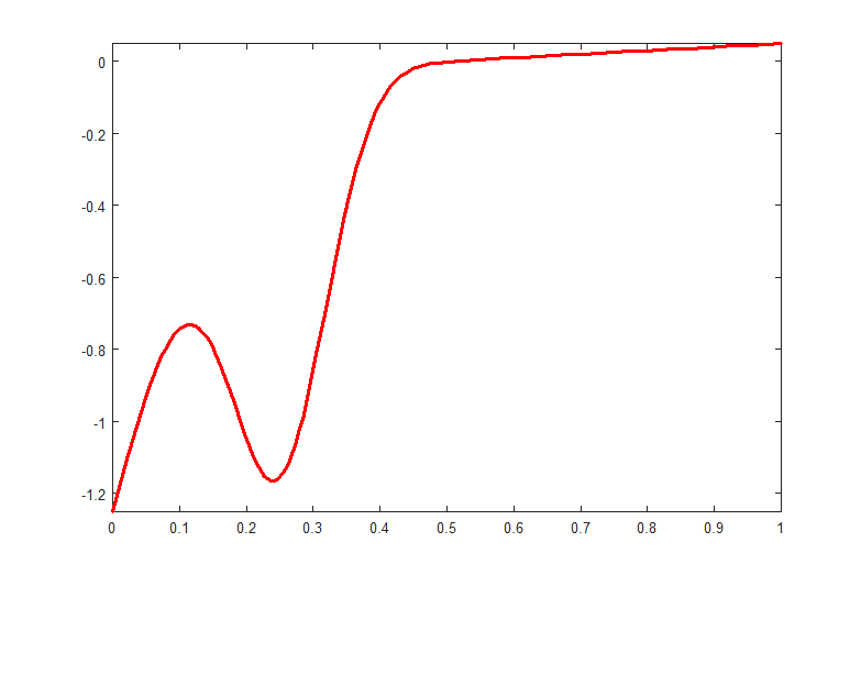
Figure 1. Plot of the regression function in Scenario 3.

Setting	Method	B-splines		P-splines
		10%	5%	10%	5%
$L^{\prime}=6$	KS bootstrap	1	0.998	1	0.9885
$N=1000$	CvM bootstrap	0.9155	0.7335	0.9975	0.9895
$\sigma=0.5$	AD bootstrap	0.985	0.9375	0.9995	0.998
$L^{\prime}=9$	KS bootstrap	0.93	0.823	0.999	0.998
$N=1000$	CvM bootstrap	0.862	0.766	0.998	0.9935
$\sigma=0.5$	AD bootstrap	0.9195	0.8085	0.9985	0.9935
$L^{\prime}=12$	KS bootstrap	0.864	0.8175	0.996	0.9885
$N=1000$	CvM bootstrap	0.8505	0.7895	0.989	0.9725
$\sigma=0.5$	AD bootstrap	0.8655	0.799	0.9885	0.974
$L^{\prime}=19$	KS bootstrap	0.639	0.5375	0.9815	0.9515
$N=1000$	CvM bootstrap	0.5295	0.395	0.9435	0.8795
$\sigma=0.5$	AD bootstrap	0.571	0.428	0.9445	0.892
$L^{\prime}=6$	KS bootstrap	1	1	1	1
$N=1000$	CvM bootstrap	1	1	1	1
$\sigma=0.25$	AD bootstrap	1	1	1	1
$L^{\prime}=9$	KS bootstrap	1	1	1	1
$N=1000$	CvM bootstrap	1	1	1	1
$\sigma=0.25$	AD bootstrap	1	1	1	1
$L^{\prime}=12$	KS bootstrap	0.9995	0.9995	1	1
$N=1000$	CvM bootstrap	0.996	0.9945	1	1
$\sigma=0.25$	AD bootstrap	1	0.996	1	1
$L^{\prime}=19$	KS bootstrap	0.996	0.986	1	1
$N=1000$	CvM bootstrap	0.9155	0.836	1	1
$\sigma=0.25$	AD bootstrap	0.955	0.891	1	1

Table 3. Tests for monotonicity in Scenario 3. Rejection rates in 2000 simulations. $L^{\prime}+1$ denotes the number of equidistant knots on $[0,1]$. $N$ denotes the number of observations in each simulation. $\sigma$ is the standard deviation in the error distribution.

The power of monotonicity tests based on this regression function is considered in [42] and a similar regression function is considered in [48]. Note that [42] considers smaller sample sizes and also smaller standard deviation of noise with $\sigma=0.1$.

Scenario 4 (analysis of power of the test). The regression function

$$m(x)=x+0.415\exp(-ax^{2}),\quad a>0.$$

and depicted in Figure 2. The left-hand side graph in Figure 2 is for the case $a=50$ and the right-hand side graph in Figure 2. In the latter case the non-monotonicity dip is smaller. These situations are considered to be challenging for monotonicity tests as these functions are somewhat close to the set of monotone functions (in any conventional metric). As expected, the power of the test depends on the value of parameter $a$ and also depends on the variance of the error. The results are summarized in Table 4.

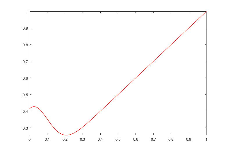
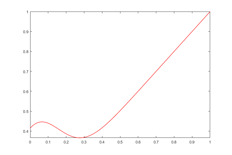
Figure 2. Plot of the regression function in Scenario 4. The left-hand side graph is for $a=50$ and the right-hand side graph is for $a=20$.

		$a=50$				$a=20$
Setting	Method	B-splines		P-splines		B-splines		P-splines
		10%	5%	10%	5%	10%	5%	10%	5%
$L^{\prime}=6$	KS	0.382	0.2425	0.575	0.423	0.25	0.139	0.338	0.216
$N=1000$	CvM	0.3385	0.2245	0.5165	0.384	0.2465	0.1335	0.311	0.212
AD $\sigma=0.5$	AD	0.434	0.228	0.6015	0.457	0.2475	0.1395	0.3355	0.221
$L^{\prime}=9$	KS	0.381	0.2545	0.572	0.4655	0.2	0.124	0.3405	0.221
$N=1000$	CvM	0.363	0.2355	0.536	0.3915	0.2055	0.132	0.3385	0.206
$\sigma=0.5$	AD	0.4735	0.3165	0.6095	0.4555	0.228	0.145	0.348	0.206
$L^{\prime}=12$	KS	0.3975	0.27	0.5995	0.4745	0.22	0.1375	0.343	0.2185
$N=1000$	CvM	0.3905	0.2565	0.5545	0.4075	0.2335	0.152	0.3215	0.2065
$\sigma=0.5$	AD	0.486	0.3505	0.614	0.5035	0.2525	0.1625	0.3415	0.2195
$L^{\prime}=19$	KS	0.4045	0.284	0.5905	0.476	0.2185	0.1235	0.3455	0.2265
$N=1000$	CvM	0.418	0.308	0.5525	0.414	0.232	0.145	0.318	0.1995
$\sigma=0.5$	AD	0.497	0.37	0.6125	0.4915	0.2485	0.155	0.341	0.2205
$L^{\prime}=6$	KS	0.9	0.8405	0.986	0.9625	0.5795	0.4605	0.756	0.6415
$N=1000$	CvM	0.8295	0.7025	0.9615	0.913	0.5895	0.4195	0.741	0.626
$\sigma=0.25$	AD	0.939	0.854	0.9835	0.9665	0.608	0.4505	0.7275	0.6295
$L^{\prime}=9$	KS	0.919	0.8385	0.986	0.9685	0.484	0.3355	0.6805	0.5645
$N=1000$	CvM	0.8355	0.7275	0.966	0.911	0.46	0.347	0.6495	0.5065
$\sigma=0.25$	AD	0.937	0.8695	0.99	0.9615	0.4995	0.374	0.6655	0.512
$L^{\prime}=12$	KS	0.9235	0.842	0.9865	0.9705	0.461	0.334	0.6785	0.5585
$N=1000$	CvM	0.863	0.756	0.97	0.9325	0.436	0.318	0.6525	0.4965
$\sigma=0.25$	AD	0.951	0.8895	0.9865	0.9705	0.492	0.3575	0.658	0.517
$L^{\prime}=19$	KS	0.925	0.8505	0.9865	0.974	0.4835	0.3505	0.698	0.585
$N=1000$	CvM	0.8835	0.802	0.9745	0.9355	0.4595	0.345	0.6625	0.495
$\sigma=0.25$	AD	0.941	0.8985	0.987	0.9695	0.486	0.3665	0.666	0.5105
$L^{\prime}=6$	KS	1	1	1	1	1	0.998	1	1
$N=1000$	CvM	1	1	1	1	0.9985	0.9965	1	1
$\sigma=0.1$	AD	1	1	1	1	0.9995	0.9975	1	1
$L^{\prime}=9$	KS	1	1	1	1	0.9935	0.9875	1	1
$N=1000$	CvM	1	1	1	1	0.9915	0.9825	1	0.9955
$\sigma=0.1$	AD	1	1	1	1	0.9915	0.9865	1	0.997
$L^{\prime}=12$	KS	1	1	1	1	0.968	0.9535	0.9995	0.998
$N=1000$	CvM	1	1	1	1	0.9539	0.932	0.9975	0.995
$\sigma=0.1$	AD	1	1	1	1	0.969	0.951	0.998	0.997
$L^{\prime}=19$	KS	1	1	1	1	0.973	0.9515	0.9995	0.9995
$N=1000$	CvM	1	1	1	1	0.9525	0.9285	0.9985	0.9955
$\sigma=0.1$	AD	1	1	1	1	0.966	0..948	0.999	0.997

Table 4. Tests for monotonicity in Scenario 4. Rejection rates in 2000 simulations. $L^{\prime}+1$ denotes the number of equidistant knots on $[0,1]$ (including 0 and 1). $N$ denotes the number of observations in each simulation. $\sigma$ is the standard deviation in the error distribution.

The power of monotonicity tests based on this regression function is examined in [42] and a similar regression function was considered in [11]. Note that [42] uses smaller sample sizes and also only $a=50$ and $\sigma=0.1$ to analyze power implications.

Scenario 5 (test for log-convexity). We take the following regression function:

$$m\left(x\right)=\exp(x^{2}),\quad x\in\left[0,1\right]\text{.}$$

The results are summarized in Table 5. In this case, the results for P-splines are the same as for B-splines as the cross-validation criterion indicated 0 as the optimal penalty parameter in the overwhelming majority of simulations.

Setting	Method	B-splines
		10%	5%
$L^{\prime}=6$	KS bootstrap	0.1045	0.0535
$N=1000$	CvM bootstrap	0.1015	0.054
$\sigma=0.25$	AD bootstrap	0.1015	0.0495
$L^{\prime}=9$	KS bootstrap	0.098	0.0435
$N=1000$	CvM bootstrap	0.1	0.0445
$\sigma=0.25$	AD bootstrap	0.1	0.048
$L^{\prime}=12$	KS bootstrap	0.1135	0.053
$N=1000$	CvM bootstrap	0.0935	0.0465
$\sigma=0.25$	AD bootstrap	0.095	0.0495

Table 5. Tests for log-convexity in Scenario 5. Rejection rates in 2000 simulations. $L^{\prime}+1$ denotes the number of equidistant knots on $[0,1]$. $N$ denotes the number of observations in each simulation. $\sigma$ is the standard deviation in the error distribution.

5.2. APPLICATIONS

1. Hospital data Here we use data on hospital finance for 332 hospitals in California in 2003. The data include many variables related to hospital finance and hospital utilization. We are interested in analyzing the effect of revenue derived from patients on administrative expenses.

Figure 3 is a scatter plot of the logarithm of patient revenue and the logarithm of administrative expenses with the fitted curve obtained using cubic B-splines with $L^{\prime}+1=5$ uniform knots in the range of values of the log of patient revenue. The fitted cure is obtained under the monotonicity restriction.

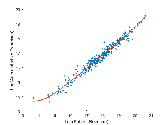
Figure 3. Hospital data. Plot of the log of administrative expenses and the log of patient revenue and the constrained (under monotonicity) fit by cubic B-splines with $L^{\prime}+1=5$ uniform knots in the domain of the log of patient revenue.

We conduct tests for the following hypotheses: (a) monotonicity; (b) convexity; (c) monotonicity and convexity.

In order to correct for heteroscedasticity of the errors, we estimate the scedastic function $\widehat{\sigma}^{2}(x)$ using residuals obtained in the unconstrained estimation using cubic B-splines with the same set of knots. The scedastic function $\widehat{\sigma}^{2}(x)$ is estimated by regressing the logarithm of the squared unconstrained residuals on a linear combination of first-order B-splines with $6$ knots in the domain of the log of patient revenue.

We then consider the constrained residuals divided by $\widehat{\sigma}(x)$ when calculating KS, CvM and AD test statistics and unconstrained residuals divided by $\widehat{\sigma}(x)$ when drawing bootstrap samples. After a bootstrap sample of residuals is drawn, we multiply each residual by the corresponding $\widehat{\sigma}(x)$ when generating a bootstrap sample of observations of the dependent variable.

We implement the testing procedure by conducting the Khmaladze transformation both from the right end of the support (as is described theoretically in this paper) and from the left end of the support and obtained extremely similar results. More specifically, we only report results when the transformation is conducted from the right end of the support.

In the case of $P$-splines, we use the same B-spline basis, take the second-order penalty and choose the penalization constant using the ordinary cross-validation criterion as in Eilers and Marx (1996). The penalty enters unconstrained optimization problems as well as constrained ones.

Tables 6-8 present results of our testing. Namely, Table 6 shows test statistics for the null hypothesis of the monotonically increasing regression function and also bootstrap critical values using both B-splines and P-splines. Table 7 presents analogous results for the null hypothesis of convexity of the regression function. Table 8 gives results for the joint null hypothesis of monotonicity and convexity.

	B-splines				P-splines
	Test statistic	Bootstrap critical value			Test statistic	Bootstrap critical value
Method		10%	5%	1%		10%	5%	1%
KS	1.0365	1.1801	1.3028	1.6393	0.7965	0.8502	0.9246	1.1044
CvM	0.2842	0.3428	0.45	0.7656	0.0614	0.1113	0.1356	0.2138
AD	1.5477	1.739	2.2068	3.5445	0.4691	0.664	0.8037	1.1031

Table 6. Hospital data. Test statistics and bootstrap critical values under the null hypothesis of monotonicity of the regression function. Bootstrap critical values are from 400 bootstrap replications.

	B-splines				P-splines
	Test statistic	Bootstrap critical value			Test statistic	Bootstrap critical value
Method		10%	5%	1%		10%	5%	1%
KS	0.9064	1.3918	1.5949	1.9306	0.7678	1.3462	1.5503	1.9284
CvM	0.1188	0.5137	0.6783	1.1675	0.1302	0.4994	0.6404	1.1974
AD	0.7103	2.7328	3.6416	7.1427	0.7241	2.5773	3.3495	7.119

Table 7. Hospital data. Test statistics and bootstrap critical values under the null hypothesis of convexity of the regression function. Bootstrap critical values are from 400 bootstrap replications.

	B-splines				P-splines
	Test statistic	Bootstrap critical value			Test statistic	Bootstrap critical value
Method		10%	5%	1%		10%	5%	1%
KS	1.218	1.4347	1.6063	1.9643	1.092	1.3568	1.6256	1.903
CvM	0.2497	0.5488	0.7375	1.4689	0.1895	0.4785	0.7751	1.221
AD	1.2513	3	3.8429	7.0125	0.9857	2.6499	3.8105	6.9091

Table 8. Hospital data. Test statistics and bootstrap critical values under the null hypothesis of both monotonicity and convexity of the regression function. Bootstrap critical values are from 400 bootstrap replications.

As we can see from Tables 6–8, we do not reject any of the three hypotheses even at 10% level.

2. Energy consumption in the Southern region of Russia.

The data are on daily energy consumption (in MWh) and average daily temperature (in Celsius) in the Southern region of Russia in the period from February 1, 2016 till January 31, 2018. The data have been downloaded from the official website of System Operator of the Unified Energy System of Russia.

We provide tests for U-shape with a switch at ${17.6}^{\circ}$ and convexity using the approaches outlined in section 2.1 in the context of Examples 2 and 1, respectively. In order to correct for heteroscedasticity of the errors, we estimate the scedastic function $\widehat{\sigma}^{2}(x)$ using residuals obtained in the unconstrained estimation using B-splines (or P-splines, respectively). The scedastic function is estimated using cubic B-splines with 6 uniform knots and in the form of

$$\sigma^{2}(x)=\left(\sum_{k=1}^{8}c_{k}B_{k,8}\right)^{2}.$$

Figure 4 gives scatter plots of the data together with fitted curves obtained under the U-shape constraint with the switch at $s_{0}={17.6}^{\circ}$. This constraint fit is obtained in accordance with the technique in section 2.1. Namely, we consider individual B-spline fits on intervals $[\underline{x},s_{0}]$ and $[s_{0},\overline{x}]$, where $\underline{x}$ and $\overline{x}$ are respectively lowest and highest values of the temperature in the sample. On each interval we use $L^{\prime}+1=5$ uniform knots. The left-hand side figure only imposes the continuity of the fitted curve at the switch point, whereas the right-hand side figure imposes continuous differentiability.

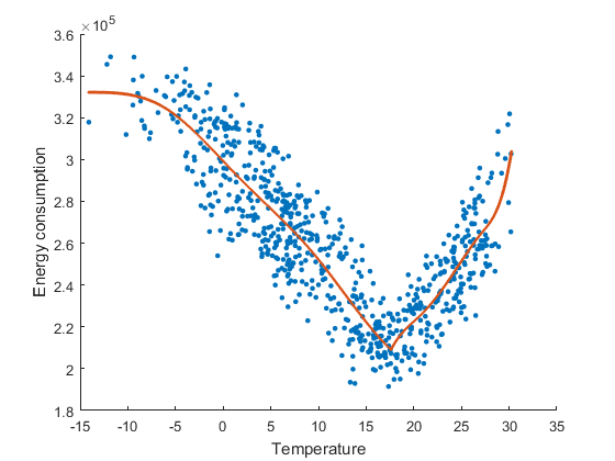
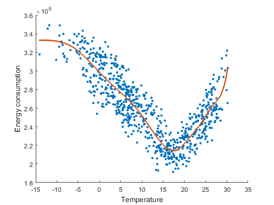
Figure 4. Energy consumption data. Plot of temperature and energy consumption and the constrained fit (under U-shape with the switch at ${17.6}^{\circ}$) using cubic B-spline with 5 uniform knots on each subinterval of temperature values. On the left-hand side the fitted curve is continuous at the switch point. On the right-hand side the fitted curve is continuously differentiable at the switch point.

Tables 9-11 present results of our testing. Namely, Table 9 shows test statistics for the null hypothesis of U-shaped regression function and also bootstrap critical values using both B-splines and P-splines in case when two B-spline curves are joined at the switch point in a continuous way. Table 10 presents analogous results for the null hypothesis of U-shaped regression function when two B-spline curves are joined at the switch point in a continuously differentiable way. Table 11 gives results for the null hypothesis of convexity. In all the cases Khmaladze’s transformation is conducted from the right end of support. he bootstrap critical values obtained on the basis of $400$ bootstrap replications. As we can see, the null hypothesis of a U-shaped relationship with the switch point at ${17.6}^{\circ}$ is not rejected at the $5\%$ level by any type of the test, whereas convexity is rejected. When testing convexity we use cubic splines with $L^{\prime}+1=7$ uniform knots on $[\underline{x},\overline{x}]$.

	B-splines				P-splines
	Test statistic	Bootstrap critical value			Test statistic	Bootstrap critical value
Method		10%	5%	1%		10%	5%	1%
KS	0.6204	1.0997	1.2139	1.4053	0.2482	0.5898	0.6199	0.7207
CvM	0.0698	0.3098	0.4048	0.5885	0.0038	0.0434	0.0498	0.0621
AD	0.5119	1.6541	2.1098	2.925	0.0647	0.397	0.4312	0.5324

Table 9. Energy consumption data. Test statistics and bootstrap critical values under the null hypothesis of U-shaped regression function with the switch as ${17.6}^{\circ}$. Two B-spline curves are joined continuously at the switch point. Bootstrap critical values are from 400 bootstrap replications.

	B-splines				P-splines
	Test statistic	Bootstrap critical value			Test statistic	Bootstrap critical value
Method		10%	5%	1%		10%	5%	1%
KS	0.8481	1.023	1.1749	1.407	0.505	0.6143	0.6524	0.7747
CvM	0.1472	0.2211	0.3247	0.5553	0.0469	0.0476	0.0542	0.0752
AD	0.9114	1.3676	1.8002	2.9199	0.2878	0.3713	0.4151	0.5547

Table 10. Energy consumption data. Test statistics and bootstrap critical values under the null hypothesis of U-shaped regression function with the switch as ${17.6}^{\circ}$. Two B-spline curves are joined smoothly at the switch point. Bootstrap critical values are from 400 bootstrap replications.

	B-splines				P-splines
	Test statistic	Bootstrap critical value			Test statistic	Bootstrap critical value
Method		10%	5%	1%		10%	5%	1%
KS	2.9812	1.1537	1.2652	1.5579	3.4626	0.5478	0.6891	1.0121
CvM	2.7713	0.3327	0.4389	0.71	3.2622	0.0402	0.0716	0.2076
AD	14.361	1.823	2.3809	3.856	17.23	0.3332	0.484	1.2158

Table 11. Energy consumption data. Test statistics and bootstrap critical values under the null hypothesis of convexity of the regression function. Bootstrap critical values are from 400 bootstrap replications.

6. CONCLUSION

This paper proposes a methodology for testing a wide range of shape properties of a regression function. The methodology relies on applying the Khmaladze’s transformation to the partial sums empirical process in a nonparametric setting where B-splines have been used to approximate the functional space under the null hypothesis. We establish that the proposed Khmaladze’s transformation eliminates the effect of nonparametric estimation and results in asymptotically pivotal testing. To the best of our knowledge, this paper is the first implementation of the Khmaladze’s transformation in a nonparametric setting.

In our main examples we considered shape constraints that can be written as inequality constraints on the coefficients of the approximating regression splines. The generality of our procedure allows to test several shape properties simultaneously. The implementation is especially easy when the inequality constraints are linear, which is the case for shape properties expressed as linear inequality constraints on the derivatives.

7. APPENDIX A

For a $M\times M$ matrix $C=\left\{c_{kj}\right\}_{k,j=1}^{M}$, $\left\|C\right\|_{E}=\sum_{k,j=1}^{M}c_{kj}^{2}$ denotes the Euclidean norm and for a $M\times N$ matrix we define the spectral norm $\left\|G\right\|$ as $\overline{\lambda}^{1/2}\left(G^{\prime}G\right)$, where $\overline{\lambda}\left(H\right)$ denotes the maximum eigenvalue of the matrix $H$. It is worth recalling the following inequality $\left\|CG\right\|_{E}\leq\left\|C\right\|_{E}\left\|G\right\|$. Finally $K$ denotes a generic finite and positive constant.

We now introduce the following notation. We shall denote the fourth cumulant of a random variable $z$ by $\kappa_{4}\left(z\right)$ and for any $x_{i}$, $i=1,...,n$, $\mathcal{I}\left(x^{1}<x_{i}<x^{2}\right)=:\mathcal{I}_{i}\left(x^{1},x^{2}\right)$. Also we define

(7.1) $$A_{L,i} = A_{L}\left(\widetilde{x}_{i}\right)\text{, \ \ \ \ }\widetilde{\boldsymbol{P}}_{i}=A_{L,i}^{+1/2}\boldsymbol{P}_{i}\text{; }\ i=1,...,n$$

$$\overline{A}_{L}\left(x\right) = D_{L}\left(x\right)A_{L}\left(x\right)D_{L}\left(x\right)\text{; \ \ }\overline{A}_{L,i}=:\overline{A}_{L}\left(\widetilde{x}_{i}\right)\text{,}$$

where $A_{L}\left(x\right)$ was given in $\left(\ref{L_x}\right)$ and

(7.2) $$D_{L}\left(x\right)=diag\left(d_{1}\left(x\right),...,d_{L}\left(x\right)\right)\text{, \ }d_{\ell}\left(x\right)=\left\{\begin{array}[]{c}0\text{ \ \ \ \ \ \ \ \ \ \ \ \ \ \ \ \ \ \ \ \ if \ \ \ \ \ \ }x<z^{\ell-1}\\ L^{-q}\left(z^{\ell}-x\right)^{-q-1/2}\ \ \ \ \text{if \ \ \ \ \ }z^{\ell-1}\leq x<z^{\ell}\\ L^{1/2}\text{ \ \ \ \ \ \ \ \ \ \ \ \ \ \ if \ \ \ \ \ \ \ }z^{\ell}\leq x\text{.}\end{array}\right.$$

Observe that when $x=:z^{k}$, that is a knot, Condition $C1$ yields that

$$\overline{A}_{L}\left(z^{k}\right)=:L~{}A_{L}\left(z^{k}\right)=diag\left(\underline{0},B_{L}\left(z^{k}\right)\right)\text{,}$$

where $\underline{0}$ is a square $k-1$ matrix of zeroes and the $L-k+1$ matrix $B_{L}\left(z^{k}\right)$ is positive definite, where the elements $B_{L,\ell_{1},\ell_{2}}\left(z^{k}\right)$ of the matrix $B_{L}\left(z^{k}\right)$ are zero if $\left|\ell_{1}-\ell_{2}\right|>q$. The latter follows because there are only $q$ splines different than zero at a given value $x$. Finally, it is worth mentioning that for $x\in\left(z^{\ell-1},z^{\ell}\right)$, $d_{\ell}\left(x\right)=Kp_{\ell,L}^{-1}\left(x;q\right)\left(z^{\ell}-x\right)^{-1/2}$ and recalling that Harville’s [52] Section 20.2 yields that $\overline{A}_{L}^{+}\left(z^{k}\right)=diag\left(\underline{0},B_{L}^{-1}\left(z^{k}\right)\right)$, where we abbreviate $p_{\ell,L}\left(x;q\right)$ by $p_{\ell,L}\left(x\right)$ in what follows.

7.1. PROOF OF THEOREM 1

We need to show $\left(\mathbf{a}\right)$ the finite dimensional distributions converge to a Gaussian random variable with covariance structure given by that of $\mathcal{U}\left(x\right)$ and $\left(\mathbf{b}\right)$ the tightness of the sequence. We begin the proof of part $\left(\mathbf{a}\right)$ showing the structure of the covariance structure of $\mathcal{M}_{n}\left(x\right)$. That is, for any $0\leq x^{1}\leq x^{2}\leq 1$,

$$E\left(\mathcal{M}_{n}\left(x^{1}\right)\mathcal{M}_{n}\left(x^{2}\right)\mid X\right) = \frac{1}{n}\sum_{i,j=1}^{n}E\left(v_{i}v_{j}\mid X\right)\mathcal{I}_{i}\left(x^{1}\right)\mathcal{I}_{j}\left(x^{2}\right)$$

$$\overset{P}{\rightarrow}\sigma_{u}^{2}F_{X}\left(x^{1}\right)\text{.}$$

Consider $i<j$ first and assume, without loss of generality, that $x_{i}<x_{j}$. When $x_{i}+n^{-\varsigma}\leq z^{k\left(x_{i}\right)}$, that is $\widetilde{x}_{i}=x_{i}$, Condition $C1$ implies that

$$E\left(C_{n,j}u_{i}\mid X\right) = 0;\text{ }E\left(C_{n,i}u_{j}\mid X\right)=\frac{\sigma_{u}^{2}}{n}\boldsymbol{P}_{j}$$

(7.4) $$E\left(C_{n,i}C_{n,j}^{\prime}\mid X\right) = \frac{\sigma_{u}^{2}}{n}A_{n,j}\text{,}$$

and hence we obtain that

(7.5) $$E\left(v_{i}v_{j}\mid X\right)=\frac{\sigma_{u}^{2}}{n}\left\{\boldsymbol{P}_{i}^{\prime}A_{n,i}^{+}A_{n,j}A_{n,j}^{+}\boldsymbol{P}_{j}-\boldsymbol{P}_{i}^{\prime}A_{n,i}^{+}\boldsymbol{P}_{j}\right\}=0$$

because Harville’s [52] Theorem 12.3.4 yields that $A_{n,j}A_{n,j}^{+}\boldsymbol{P}_{j}=\boldsymbol{P}_{j}$. On the other hand when $x_{i}+n^{-\varsigma}>z^{k\left(x_{i}\right)}$, that is $\widetilde{x}_{i}\not=x_{i}$ and $x_{j}>z^{k\left(x_{i}\right)}$, $\left(\ref{th_1_a}\right)$ holds true which implies $\left(\ref{th_1_b}\right)$. Finally when $z^{k\left(x_{i}\right)}-n^{-\varsigma}<x_{i},x_{j}\leq z^{k\left(x_{i}\right)}$, we obtain that

$$E\left(v_{i}v_{j}\mid X\right) = \frac{\sigma_{u}^{2}}{n}\boldsymbol{P}_{i}^{\prime}A_{n}^{+}\left(z^{k\left(x_{i}\right)}\right)\boldsymbol{P}_{j}\mathcal{I}\left(z^{k\left(x_{i}\right)}-\frac{1}{n^{\varsigma}}<x_{i},x_{j}\leq z^{k\left(x_{i}\right)}\right)$$

$$= :\vartheta_{n}\left(i,j;X\right)\text{.}$$

Observe that in this case we have

(7.6) $$E\left\|E\left(v_{i}v_{j}\mid X\right)\right\|=O\left(Ln^{-1-2\varsigma}\right)$$

because Lemmas 3 and 4 imply that

(7.7) $$\underline{\lambda}\left(\inf_{x\in\left[0,1\right]}A_{L}^{+1/2}\left(x\right)A_{n}\left(x\right)A_{L}^{+1/2}\left(x\right)\right)>\delta>0$$

with probability approaching one, where $\lambda$$\left(G\right)$ denotes the minimum eigenvalue of the matrix $G$, Lemma 2 implies that $E\left\|\widetilde{\boldsymbol{P}}_{i}\right\|^{2}=O\left(L\right)$ and

(7.8) $$E\left(\mathcal{I}\left(z^{k\left(x_{i}\right)}-n^{-\varsigma}<x_{i}\leq z^{k\left(x_{i}\right)}\right)\right)=O\left(n^{-\varsigma}\right)\text{.}$$

Next, when $i=j$, proceeding as above we obtain that

$$E\left(v_{i}v_{j}\mid X\right)=\sigma_{u}^{2}\left(1-\frac{\boldsymbol{P}_{i}^{\prime}A_{n,i}^{+}\boldsymbol{P}_{i}}{n}\right)\text{.}$$

Observe that, denoting $A_{n,i}^{\ast}=A_{n,i}-\boldsymbol{P}_{i}\boldsymbol{P}_{i}^{\prime}/n$, we have that

$$1-\frac{\boldsymbol{P}_{i}^{\prime}A_{n,i}^{+}\boldsymbol{P}_{i}}{n}=1-2\frac{\boldsymbol{P}_{i}^{\prime}A_{n,i}^{+}\boldsymbol{P}_{i}}{n}+\left(\frac{\boldsymbol{P}_{i}^{\prime}A_{n,i}^{+}\boldsymbol{P}_{i}}{n}\right)^{2}+\frac{\boldsymbol{P}_{i}^{\prime}A_{n,i}^{+}A_{n,i}^{\ast}A_{n,i}^{+}\boldsymbol{P}_{i}}{n}>0\text{.}$$

So, we conclude that the left side of $\left(\ref{pth1_1}\right)$ is, for any $0\leq x^{1}\leq x^{2}\leq 1$,

(7.9) $$\frac{\sigma_{u}^{2}}{n}\sum_{i=1}^{n-1}\left(1-\frac{\boldsymbol{P}_{i}^{\prime}A_{n,i}^{+}\boldsymbol{P}_{i}}{n}\right)\mathcal{I}_{i}\left(x^{1}\right)+\frac{\sigma_{u}^{2}}{n}\sum_{i\neq j}^{n-1}\vartheta_{n}\left(i,j;X\right)\mathcal{I}_{i}\left(x^{1}\right)\text{.}$$

The second term of $\left(\ref{Theo1_1}\right)$ is $o_{p}\left(1\right)$ because $\left(\ref{e_v_i_vj}\right)$ implies that its first absolute moment is $O\left(L/n^{2\varsigma}\right)=o\left(1\right)$ since $\varsigma>1/2$ and Condition $C3$. The first term of $\left(\ref{Theo1_1}\right)$ is also $o_{p}\left(1\right)$ as we now show. Using the inequality $\mathcal{I}_{i}\left(x^{1}\right)\leq\sum_{k=1}^{k\left(x^{1}\right)-1}\mathcal{I}_{i}\left(z^{k};z^{k+1}\right)$, we obtain that

(7.10) $$E\left(\frac{1}{n^{2}}\sum_{i=1}^{n-1}\widetilde{\boldsymbol{P}}_{i}^{\prime}\left(A_{L,i}^{+1/2}A_{n,i}A_{L,i}^{+1/2}\right)^{+}\widetilde{\boldsymbol{P}}_{i}\mathcal{I}_{i}\left(x^{1}\right)\right)$$

$$\leq \sum_{k=1}^{k\left(x^{1}\right)-1}E\left(\frac{1}{n^{2}}\sum_{i=1}^{n-1}\widetilde{\boldsymbol{P}}_{i}^{\prime}\left(A_{L,i}^{+1/2}A_{n,i}A_{L,i}^{+1/2}\right)^{+}\widetilde{\boldsymbol{P}}_{i}\mathcal{I}_{i}\left(z^{k};z^{k+1}\right)\right)$$

$$= \frac{K}{n^{2}}\sum_{k=1}^{k\left(x^{1}\right)-1}\sum_{i=1}^{n}E\left\|\widetilde{\boldsymbol{P}}_{i}\mathcal{I}_{i}\left(z^{k};z^{k+1}\right)\right\|^{2}=O\left(\frac{L}{n}\right)\text{,}$$

by $\left(\ref{A_inv}\right)$ and because $E\left\|\widetilde{\boldsymbol{P}}_{i}\mathcal{I}_{i}\left(z^{k};z^{k+1}\right)\right\|^{2}=O\left(1\right)$ by Lemma 2, cf. $\left(\ref{Lemma2_4}\right)$. So, we conclude that $\left(\ref{pth1_1}\right)$ holds true as it is well known that, under Conditions $C1$ and then $C3$,

$$\sigma_{u}^{2}\frac{1}{n}\sum_{i=1}^{n}\mathcal{I}_{i}\left(x\right)\left(1+\frac{L}{n}\right)\overset{P}{\rightarrow}\sigma_{u}^{2}F_{X}\left(x\right)\text{.}$$

To complete part $\left(\mathbf{a}\right)$, it suffices to show the asymptotic Gaussianity of $\mathcal{M}_{n}\left(x\right)$ for a fixed $x$ due to Cramér-Wold device. First, we have already shown that

$$\sum_{i=1}^{n}E\left(\upsilon_{in}^{2}\left(x\right)\mid X\right)\overset{P}{\rightarrow}1\text{,}$$

where by construction $\upsilon_{in}\left(x\right)=:\sigma_{u}^{-1}F_{X}^{-1/2}\left(x\right)\mathcal{I}_{i}\left(x\right)v_{i}/n^{1/2}$ is a martingale difference triangular array of r.v.’s. So, it remains to show the Lindeberg’s condition for which a sufficient condition is

(7.11) $$\sum_{i=1}^{n}E\left|\upsilon_{in}\left(x\right)\right|^{4}=o\left(1\right)\text{.}$$

But the latter holds true because $\left(\ref{A_inv}\right)$ yields that

$$E\left\|\boldsymbol{P}_{i}^{\prime}A_{n,i}^{+}C_{n,i}\mathcal{I}_{i}\left(x\right)\right\|^{4}\leq E\left\|\widetilde{\boldsymbol{P}}_{i}\right\|^{4}E\left\|\frac{1}{n}\sum_{j=1}^{n}\widetilde{\boldsymbol{P}}_{j}u_{j}\mathcal{J}_{j}\left(\widetilde{x}_{i}\right)\right\|^{4}=O\left(\frac{L^{4}}{n^{2}}\right)\text{,}$$

since Lemma 2 implies that $E\left\|\widetilde{\boldsymbol{P}}_{i}\right\|^{4}=O\left(L^{2}\right)$. So, $\left(\ref{v_in}\right)$ holds true by Condition $C3$, which concludes the proof of part $\left(\mathbf{a}\right)$.

$\left(\mathbf{b}\right)$ Tightness follows by Lemmas 4 and 5 and using the same arguments as those for the proof of Billingsley’s [8] Theorem 22.1, see also Wu’s [92] Lemma 14, which completes the proof of the theorem. Observe that, for any $\delta>0$, $\delta\sum_{k\in\mathbb{Z}}\sup_{x\in\left(k\delta,\left(k+1\right)\delta\right)}f_{X}\left(x\right)<K$ following Lemma 4 of Wu [92].

7.2. PROOF OF THEOREM 2

We shall show that, uniformly in $x\in\left[0,1\right]$,

(7.12) $$\widetilde{\mathcal{M}}_{n}\left(x\right)-\mathcal{M}_{n}\left(x\right)=o_{p}\left(1\right)\text{.}$$

Because $\left(\ref{res_con}\right)$ yields that $\widehat{u}_{i}-u_{i}=m^{bias}\left(x_{i}\right)-\boldsymbol{P}_{i}^{\prime}\left(\widehat{b}-\beta\right)$, we have that the left side of $\left(\ref{m_dif}\right)$ is

(7.13) $$\frac{1}{n^{1/2}}\sum_{i=1}^{n}m^{bias}\left(x_{i}\right)\mathcal{I}_{i}\left(x\right)-\frac{1}{n^{1/2}}\sum_{i=1}^{n}\left\{\frac{\boldsymbol{P}_{i}^{\prime}A_{n,i}^{+}}{n}\sum_{k=1}^{n}\boldsymbol{P}_{k}m^{bias}\left(x_{k}\right)\mathcal{J}_{k}\left(\widetilde{x}_{i}\right)\right\}\mathcal{I}_{i}\left(x\right)$$

since the contribution due to $\boldsymbol{P}_{i}^{\prime}\left(\widehat{b}-\beta\right)$ is zero by Lemma 1.

Now the first term of $\left(\ref{m_dif2}\right)$ is $o_{p}\left(1\right)$ by Condition $C3$ and that Agarwal and Studden’s [2] Theorems 3.1 and 4.1, see also Zhou et al. $\left(1998\right)$, yields that $Em^{bias}\left(x_{i}\right)=O\left(L^{-3}\right)$, whereas together with Lemma 4 and $\left(\ref{A_inv}\right)$, we obtain that the second term is, with probability approaching $1$, bounded by

$$\frac{K}{L^{3}n^{1/2}}\sum_{i=1}^{n}\left\{\left\|\widetilde{\boldsymbol{P}}_{i}\right\|\frac{1}{n}\sum_{k=1}^{n}\left\|\widetilde{\boldsymbol{P}}_{k}\right\|\right\}=O_{p}\left(n^{1/2}/L^{2}\right)=o\left(1\right)$$

by Markov’s inequality and Lemma 2 and then Condition $C3$. This completes the proof of the theorem. $\blacksquare$

7.3. PROOF OF PROPOSITION 1

First, using $\left(\ref{res_con}\right)$, we have that

$$\widehat{u}_{i}^{2} = u_{i}^{2}+m^{bias}\left(x_{i}\right)^{2}+\left(\widehat{b}-\beta\right)^{\prime}\boldsymbol{P}_{i}\boldsymbol{P}_{i}^{\prime}\left(\widehat{b}-\beta\right)$$

$$+2u_{i}m^{bias}\left(x_{i}\right)+2u_{i}\boldsymbol{P}_{i}^{\prime}\left(\widehat{b}-\beta\right)+2m^{bias}\left(x_{i}\right)\boldsymbol{P}_{i}^{\prime}\left(\widehat{b}-\beta\right)\text{.}$$

So, by Cauchy-Schwarz’s inequality, it suffices to show that

(7.14) $$\left(\widehat{b}-\beta\right)^{\prime}\frac{1}{n}\sum_{i=1}^{n}\boldsymbol{P}_{i}\boldsymbol{P}_{i}^{\prime}\left(\widehat{b}-\beta\right)\text{ \ and }\frac{1}{n}\sum_{i=1}^{n}m^{bias}\left(x_{i}\right)^{2}$$

are$\ o_{p}\left(1\right)$ because $n^{-1}\sum_{i=1}^{n}u_{i}^{2}-\sigma_{u}^{2}=o_{p}\left(1\right)$. Now, the norm of the first expression in $\left(\ref{a1}\right)$ is $O_{p}\left(L^{1/2}/n\right)=o_{p}\left(1\right)$ because

$$E\left(\left(A_{L}\left(0\right)^{-1/2}\frac{1}{n}\sum_{i=1}^{n}\mathbf{P}_{i}u_{i}\right)\left(A_{L}\left(0\right)^{-1/2}\frac{1}{n}\sum_{i=1}^{n}\mathbf{P}_{i}u_{i}\right)^{\prime}\mid X\right)=\frac{\sigma_{u}^{2}}{n}I_{L}$$

and $\left\|I_{L}\right\|_{E}^{2}=L$. Note that by Lemma 3, $A_{n}\left(0\right)$ is invertible with probability approaching $1$ since $A_{L}\left(0\right)$ is. On the other hand, the second expression in $\left(\ref{a1}\right)$ is $o_{p}\left(1\right)$ by Agarwal and Studden’s [2] Theorems 3.1 and 4.1 and then Condition $C3$. This completes the proof of the proposition. $\blacksquare$

7.4. PROOF OF THEOREM 3

In this proof, for the sake of notation simplicity, we will write $\beta$ and $\widehat{b}$ instead of $\beta_{-\ell_{0}}$ and $\widehat{b}_{-\ell_{0}}$, respectively.

Let

$$G\left(x;\beta\right)=:\frac{\partial\widetilde{P}_{i}\left(x;\beta\right)}{\partial\beta^{\prime}}\quad\text{and}\quad G_{i}\left(\beta\right)=:G_{i}\left(x_{i};\beta\right).$$

From the definition of $\widetilde{P}_{i}\left(x;\beta\right)$, it follows that $G\left(x;\beta\right)=H(\beta)p_{\ell_{0}}(x)$, where $H(\beta)$ is the $(L-1)\times(L-1)$ Hessian of $h(\beta)$, whose norm is finite.

Then, employing the form of our model and the approximation, by Taylor’s approximation to $g(\cdot)$, we write

$$\widehat{u}_{i} = u_{i}-\left(g\left(x_{i};\widehat{b}\right)-g\left(x_{i};\beta\right)\right)+(m(x_{i})-g\left(x_{i};\beta\right))$$

$$= u_{i}-\left(\widehat{b}-\beta\right)^{\prime}\widetilde{P}_{i}\left(\beta\right)+\frac{1}{2}\left(\widehat{b}-\beta\right)^{\prime}G_{i}\left(\widetilde{b}\right)\left(\widehat{b}-\beta\right)+\left(m(x_{i})-g\left(x_{i};{\beta}\right)\right)\text{, }$$

where $\widetilde{b}$ is an intermediate point between $\beta$ and $\widehat{b}$.

So, it suffices to examine the contribution due to the following four terms:

$$\mathcal{A}_{1,n}\left(x;\widehat{b}\right) = :\frac{1}{n^{1/2}}\sum_{i=1}^{n}\left\{u_{i}-\widetilde{P}_{i}^{\prime}\left(\widehat{b}\right)\mathcal{D}_{n}^{+}\left(\widehat{b};i\right)\sum_{k=1}^{n}\widetilde{P}_{k}\left(\widehat{b}\right)u_{k}\mathcal{J}_{k}\left(\widetilde{x}_{i}\right)\right\}\mathcal{I}_{i}(x)$$

$$\mathcal{A}_{2,n}\left(x;\widehat{b}\right) = :\frac{1}{n^{1/2}}\sum_{i=1}^{n}\left\{\widetilde{P}_{i}^{\prime}\left(\beta\right)-\widetilde{P}_{i}^{\prime}\left(\widehat{b}\right)\mathcal{D}_{n}^{+}\left(\widehat{b};i\right)\sum_{k=1}^{n}\widetilde{P}_{k}\left(\widehat{b}\right)\widetilde{P}_{k}^{\prime}\left(\beta\right)\mathcal{J}_{k}\left(\widetilde{x}_{i}\right)\right\}\mathcal{I}_{i}(x)\left(\widehat{b}-\beta\right)$$

$$\mathcal{A}_{3,n}\left(x;\widehat{b}\right) = :\left(\widehat{b}-\beta\right)^{\prime}\frac{1}{n^{1/2}}\sum_{i=1}^{n}\mathcal{I}_{i}(x)G_{i}\left(\widetilde{b}\right)\left(\widehat{b}-\beta\right)$$

$$-\frac{1}{n^{1/2}}\sum_{i=1}^{n}\widetilde{P}_{i}^{\prime}\left(\widehat{b}\right)\mathcal{D}_{n}^{+}\left(\widehat{b};i\right)\frac{1}{n}\left\{\sum_{k=1}^{n}\widetilde{P}_{k}\left(\widehat{b}\right)\left(\widehat{b}-\beta\right)^{\prime}G_{k}\left(\widetilde{b}\right)\left(\widehat{b}-\beta\right)\mathcal{J}_{k}\left(\widetilde{x}_{i}\right)\right\}\mathcal{I}_{i}(x)\text{,}$$

$$\mathcal{A}_{4,n}\left(\widehat{b}\right) = :\frac{1}{n^{1/2}}\sum_{i=1}^{n}\left\{m^{bias}\left(x_{i}\right)-\widetilde{P}_{i}^{\prime}\left(\widehat{b}\right)\mathcal{D}_{n}^{+}\left(\widehat{b};i\right)\frac{1}{n}\sum_{k=1}^{n}\left(m^{bias}\left(x_{k}\right)\right)\mathcal{J}_{k}\left(\widetilde{x}_{i}\right)\right\}\mathcal{I}_{i}(x),$$

with $m(x_{i})-g\left(x_{i};{\beta}\right)=:m^{bias}\left(x_{i}\right)$. Also introduce the following:

$$\mathcal{A}_{1,n}\left(x;{\beta}\right) = :\frac{1}{n^{1/2}}\sum_{i=1}^{n}\left\{u_{i}-\widetilde{P}_{i}^{\prime}\left({\beta}\right)\mathcal{D}_{n}^{+}\left({\beta};i\right)\sum_{k=1}^{n}\widetilde{P}_{k}\left({\beta}\right)u_{k}\mathcal{J}_{k}\left(\widetilde{x}_{i}\right)\right\}\mathcal{I}_{i}(x),$$

$$\mathcal{A}_{2,n}\left(x;\beta\right) = :\frac{1}{n^{1/2}}\sum_{i=1}^{n}\left\{\widetilde{P}_{i}^{\prime}\left(\beta\right)-\widetilde{P}_{i}^{\prime}\left({\beta}\right)\mathcal{D}_{n}^{+}\left({\beta};i\right)\sum_{k=1}^{n}\widetilde{P}_{k}\left({\beta}\right)\widetilde{P}_{k}^{\prime}\left(\beta\right)\mathcal{J}_{k}\left(\widetilde{x}_{i}\right)\right\}\mathcal{I}_{i}(x)\left(\widehat{b}-\beta\right),$$

$$\mathcal{A}_{3,n}\left(x;{\beta}\right) = :\left(\widehat{b}-\beta\right)^{\prime}\frac{1}{n^{1/2}}\sum_{i=1}^{n}\mathcal{I}_{i}(x)G_{i}\left(\widetilde{b}\right)\left(\widehat{b}-\beta\right)$$

$$-\frac{1}{n^{1/2}}\sum_{i=1}^{n}\widetilde{P}_{i}^{\prime}\left({\beta}\right)\mathcal{D}_{n}^{+}\left({\beta};i\right)\frac{1}{n}\left\{\sum_{k=1}^{n}\widetilde{P}_{k}\left({\beta}\right)\left(\widehat{b}-\beta\right)^{\prime}G_{k}\left(\widetilde{b}\right)\left(\widehat{b}-\beta\right)\mathcal{J}_{k}\left(\widetilde{x}_{i}\right)\right\}\mathcal{I}_{i}(x).$$

We shall first examine the behaviour of $\mathcal{A}_{q,n}\left(x;\beta\right)$, $q=1,2,3$, and then we shall show that, uniformly in $x$, $\mathcal{A}_{q,n}\left(x;\widehat{b}\right)-\mathcal{A}_{q,n}\left(x;\beta\right)=o_{p}\left(1\right)$.

Proceeding as with the proof of Theorem 1, we can establish

$$\mathcal{A}_{1,n}\left(\beta\right)\overset{weakly}{\Rightarrow}\mathcal{U}\left(x\right).$$

It is also obvious that $\mathcal{A}_{2,n}\left(x;\beta\right)=0$. Now we want to show that

$$\sup_{x}\left|\mathcal{A}_{3,n}\left(x;\beta\right)\right|=o_{p}\left(1\right).$$

To that end, we shall look at

$$\mathcal{C}_{1,n}\left(x;\beta\right) = :\left(\widehat{b}-\beta\right)^{\prime}\left\{\frac{1}{n^{1/2}}\sum_{i=1}^{n}\mathcal{I}_{i}(x)G_{i}\left(\widetilde{b}\right)\right\}\left(\widehat{b}-\beta\right)$$

$$\mathcal{C}_{2,n}\left(x;\beta\right) = :\frac{1}{n^{1/2}}\sum_{i=1}^{n}\widetilde{P}_{i}^{\prime}\left(\beta\right)\mathcal{D}_{n}^{+}\left(\beta;i\right)\left\{\left(\sum_{k=1}^{n}\widetilde{P}_{k}\left(\beta\right)\left(\widehat{b}-\beta\right)^{\prime}G_{k}\left(\widetilde{b}\right)\left(\widehat{b}-\beta\right)\mathcal{J}_{k}\left(\widetilde{x}_{i}\right)\right)\right\}\mathcal{I}_{i}(x)\text{.}$$

We already know that $\widehat{b}-\beta=O_{p}\left(\left(L/n\right)^{1/2}\right)$. So, by definition of $G\left(x;\beta\right)$, we obtain that

$$\left\|\mathcal{C}_{1,n}\left(x;\beta\right)\right\| = \left\|H\left(\widetilde{b}\right)\right\|\left|\frac{1}{n}\sum_{i=1}^{n}Lp_{\ell_{0}}\left(x_{i}\right)\mathcal{I}_{i}(x)\right|O_{p}\left(\frac{1}{n^{1/2}}\right)$$

$$= \left\|H\left(\widetilde{b}\right)\right\|\frac{1}{n}\sum_{i=1}^{n}\left|Lp_{\ell_{0}}\left(x_{i}\right)\right|O_{p}\left(\frac{1}{n^{1/2}}\right)$$

$$= :O_{p}\left(n^{-1/2}\right)\text{,}$$

because $E\left|Lp_{\ell_{0}}\left(x_{i}\right)\right|\leq K$. So, because the last displayed expression yields that

$$\sup_{x}\left|\mathcal{C}_{1,n}\left(x;\beta\right)\right|=O_{p}\left(n^{-1/2}\right)\text{.}$$

Next, we examine $\mathcal{C}_{2,n}\left(x;\beta\right)$. Again, from the definition of $G\left(x;\beta\right)$ we have that

$$\left(\widehat{b}-\beta\right)^{\prime}G_{k}\left(\widetilde{b}\right)\left(\widehat{b}-\beta\right)=\left(\widehat{b}-\beta\right)^{\prime}H\left(\widetilde{b}\right)\left(\widehat{\beta}-\beta\right)p_{\ell_{0}}\left(x_{k}\right)\text{.}$$

From the fact that $\widehat{b}-\beta=O_{p}\left(\left(L/n\right)^{1/2}\right)$ we can conclude that

$$\mathcal{C}_{2,n}\left(\beta\right)=C\frac{L}{n^{3/2}}\sum_{i=1}^{n}\widetilde{P}_{i}^{\prime}\left(\beta\right)\mathcal{D}_{n}^{+}\left(\beta;i\right)\left\{\sum_{k=1}^{n}\widetilde{P}_{k}\left(\beta\right)p_{\ell_{0}}\left(x_{k}\right)\iota_{L}^{\prime}H\left(\widetilde{b}\right)\iota_{L}\mathcal{J}_{k}\left(\widetilde{x}_{i}\right)\right\}\mathcal{I}_{i}(x)\text{,}$$

where $\iota_{L}=(1,\ldots,1)^{\prime}$ and $C$ is some positive constant.

We can establish that $\underline{\lambda}\left(\frac{L}{n}\mathcal{D}_{n}\left(\beta;i\right)\right)>0$ as this is what we have essentially in expression $\left(\ref{A_inv}\right)$ in the Appendix of the paper. Also note that

$$E\left(L^{1/2}\widetilde{P}_{i}^{\prime}\left(\beta\right)\right) \simeq L^{-1/2}\left(1,...,1\right);$$

$$E\left(L^{1/2}\widetilde{P}_{k}\left(\beta\right)p_{\ell_{0}}\left(x_{k}\right)\right) \simeq L^{-1/2}\left(d_{1,h},...,d_{L,h}\right),^{\prime}$$

where $d_{\ell,h}$, $\ell\neq\ell_{0}$, is a 0/1 variable which takes the values of 1 if and only if the function $h$ does depend on $\beta_{\ell}$. For instance, in the case of HA-convexity, which was given as an example, $h$ would depend only on parameters $\beta_{\ell_{0}-1}$ and $\beta_{\ell_{0}-2}$ and, thus, we would only have $d_{\ell_{0}-1,h}=1$ and $d_{\ell_{0}-2,h}=1$ whereas the rest of such indicators would be zero.

In this case we would have

$$\mathcal{C}_{2,n}\left(x;\beta\right)=O_{p}\left(n^{-1/2}\right)$$

once we observe that $L^{-1/2}\left(1,...,1\right)L^{-1/2}\left(d_{1,h},...,d_{L,h}\right)^{\prime}\simeq L^{-1}$.

If $h$ depends on parameters whose number is growing at the rate $L^{1/2}$, then we would have

$$\mathcal{C}_{2,n}\left(x;\beta\right)=O_{p}\left(\left(L/n\right)^{1/2}\right)$$

since now $L^{-1/2}\left(1,...,1\right)L^{-1/2}\left(d_{1,h},...,d_{L,h}\right)^{\prime}\simeq L^{-1/2}$

Of course, in the scenario when $h$ depends on all the other parameters, we have that $L^{-1/2}\left(1,...,1\right)L^{-1/2}\left(d_{1,h},...,d_{L,h}\right)^{\prime}\simeq 1,$which yields that

$$\mathcal{C}_{2,n}\left(x;\beta\right)=O_{p}\left(\left(L^{2}/n\right)^{1/2}\right)\text{,}$$

which by Condition $C3$, it is $o_{p}\left(1\right)$.

Now we show that

$$\mathcal{A}_{q,n}\left(x;\widehat{b}\right)-\mathcal{A}_{q,n}\left(x;\beta\right)=o_{p}\left(1\right)\text{, \ \ \ }q=1,2,3\text{.}$$

For that purpose, observe that by mean value theorem, we have that

(7.15) $$\widetilde{P}_{i}\left(\widehat{b}\right)-\widetilde{P}_{i}\left(\beta\right)=H\left(\widetilde{b}\right)\left(\widehat{b}-\beta\right)p_{\ell_{0}}\left(x_{i}\right)=O_{p}\left(\left(Ln\right)^{-1//2}\right)$$

because $\sup_{\beta}\left\|H\left(\beta\right)\right\|\leq K$, $\widehat{b}-\beta=O_{p}\left(\left(L/n\right)^{1/2}\right)$ and $E\left\|p_{\ell_{0}}\left(x_{k}\right)\right\|=O\left(L^{-1}\right)$.

Next, we examine the behaviour of $\mathcal{D}_{n}^{+}\left(\widehat{b};i\right)-\mathcal{D}_{n}^{+}\left(\beta;i\right)$. By the mean value theorem and standard algebra, we have that

$$\mathcal{D}_{n}\left(\widehat{b};i\right) = \mathcal{D}_{n}\left(\beta;i\right)+2H\left(\widetilde{b}\right)\left(\widehat{b}-\beta\right)\sum_{k=1}^{n}\widetilde{P}_{k}\left(\beta\right)p_{\ell_{0}}\left(x_{k}\right)\mathcal{J}_{k}\left(\widetilde{x}_{i}\right)$$

$$+H\left(\widetilde{\beta}\right)\left(\widehat{b}-\beta\right)\left(\sum_{k=1}^{n}p_{\ell_{0}}^{2}\left(x_{k}\right)\mathcal{J}_{k}\left(\widetilde{x}_{i}\right)\right)\left(\widehat{b}-\beta\right)^{\prime}H^{\prime}\left(\widetilde{b}\right)\text{,}$$

where $\widetilde{b}$ is an intermediate point between $\beta$ and $\widehat{b}$.

The norm of the third term on the right is $O_{p}\left(1\right)$ whereas the second term on the right is $O_{p}\left(\left(n/L\right)^{1/2}\right)$. So, using the pseudo inverse of sum of matrices formula, it is easily seen that

(7.16) $$\mathcal{D}_{n}^{+}\left(\widehat{b};i\right)-\mathcal{D}_{n}^{+}\left(\beta;i\right)=O_{p}\left(\left(n/L\right)^{1/2}\right)\text{.}$$

Now, we examine $\mathcal{A}_{q,n}\left(x;\widehat{b}\right)-\mathcal{A}_{q,n}\left(x;\beta\right)$, $q=1,2,3$. Let’s examine e.g. the behaviour $\mathcal{A}_{1,n}\left(x;\widehat{b}\right)-\mathcal{A}_{1,n}\left(x;\beta\right)$. By definition, it is

$$\mathcal{A}_{1,n}\left(x;\widehat{b}\right)-\mathcal{A}_{1,n}\left(x;\beta\right) = \frac{1}{n^{1/2}}\sum_{i=1}^{n}\left\{\widetilde{P}_{i}^{\prime}\left(\widehat{b}\right)\mathcal{D}_{n}^{+}\left(\widehat{b};i\right)\sum_{k=1}^{n}\widetilde{P}_{k}\left(\widehat{b}\right)u_{k}\mathcal{J}_{k}\left(\widetilde{x}_{i}\right)\right.$$

$$\text{ \ \ \ \ \ \ \ \ \ \ \ \ \ \ }\left.-\widetilde{P}_{i}^{\prime}\left(\beta\right)\mathcal{D}_{n}^{+}\left(\beta;i\right)\sum_{k=1}^{n}\widetilde{P}_{k}\left(\beta\right)u_{k}\mathcal{J}_{k}\left(\widetilde{x}_{i}\right)\right\}\mathcal{I}_{i}(x)\text{.}$$

It suffices to show that, uniformly in $x$,

$$\left(\mathbf{i}\right)\text{ \ \ }\frac{1}{n^{1/2}}\sum_{i=1}^{n}\left\{\left(\widetilde{P}_{i}\left(\widehat{b}\right)-\widetilde{P}_{i}\left(\beta\right)\right)^{\prime}\mathcal{D}_{n}^{+}\left(\beta;i\right)\sum_{k=1}^{n}\widetilde{P}_{k}\left(\beta\right)u_{k}\mathcal{J}_{k}\left(\widetilde{x}_{i}\right)\right\}\mathcal{I}_{i}(x) = o_{p}\left(1\right)$$

$$\left(\mathbf{ii}\right)\text{ \ \ }\frac{1}{n^{1/2}}\sum_{i=1}^{n}\left\{\widetilde{P}_{i}^{\prime}\left(\beta\right)\mathcal{D}_{n}^{+}\left(\beta;i\right)\sum_{k=1}^{n}\left(\widetilde{P}_{k}\left(\widehat{b}\right)-\widetilde{P}_{k}\left(\beta\right)\right)u_{k}\mathcal{J}_{k}\left(\widetilde{x}_{i}\right)\right\}\mathcal{I}_{i}(x) = o_{p}\left(1\right)$$

$$\left(\mathbf{iii}\right)\text{ \ \ }\frac{1}{n^{1/2}}\sum_{i=1}^{n}\left\{\widetilde{P}_{i}^{\prime}\left(\beta\right)\left[\mathcal{D}_{n}^{+}\left(\widehat{b};i\right)-\mathcal{D}_{n}^{+}\left(\beta;i\right)\right]\sum_{k=1}^{n}\widetilde{P}_{k}\left(\beta\right)u_{k}\mathcal{J}_{k}\left(\widetilde{x}_{i}\right)\right\}\mathcal{I}_{i}(x) = o_{p}\left(1\right)\text{.}$$

The proof of (i)-(iii) follows quite easily based on $\left(\ref{3}\right)$ and $\left(\ref{5}\right)$, and that we have already shown that

$$\mathcal{D}_{n}^{+1/2}\left(\beta;i\right)\sum_{k=i+1}^{n}\widetilde{P}_{k}\left(\beta\right)u_{k} = O_{p}\left(L^{1/2}\right)\text{.}$$

$$\underline{\lambda}\left(\frac{L}{n}\mathcal{D}_{n}\left(\beta;i\right)\right) > 0\text{ \ with probability }1\text{.}$$

Analogously, we can easily establish that $\mathcal{A}_{q,n}\left(x;\widehat{b}\right)-\mathcal{A}_{q,n}\left(x;\beta\right)=o_{p}(1)$. Note that $\mathcal{A}_{4,n}\left(x;\widehat{b}\right)$ can be written as $\frac{1}{n^{1/2}}\sum_{i=1}^{n}m^{bias}(x_{i})\mathcal{I}_{i}(x)$ and in the same way as in the proof of Theorem 2 can be shown to be $o_{p}(1)$. $\blacksquare$

7.5. PROOF OF THEOREM 4

Define

$$\mathcal{M}_{n}^{\ast}\left(x\right)=:\frac{1}{n^{1/2}}\sum_{i=1}^{n}v_{i}^{\ast}\mathcal{I}_{i}\left(x\right)\text{,}$$

where $v_{i}^{\ast}=u_{i}^{\ast}-\boldsymbol{P}_{i}^{\prime}A_{n,i}^{+}C_{n,i}^{\ast}$ and $C_{n,i}^{\ast}=:n^{-1}\sum_{k=1}^{n}\boldsymbol{P}_{k}u_{k}^{\ast}\mathcal{J}_{k}\left(\widetilde{x}_{i}\right)$. The proof is completed if we show that, (in probability),

$$\left(\mathbf{a}\right)\text{ }\mathcal{M}_{n}^{\ast}\left(x\right)\overset{weakly}{\Rightarrow}\mathcal{B}\left(F_{X}\left(x\right)\right)$$

$$\left(\mathbf{b}\right)\text{ }\sup_{x\in\left(0,1\right)}\left|\widetilde{\mathcal{M}}_{n}^{\ast}\left(x\right)-\mathcal{M}_{n}^{\ast}\left(x\right)\right|=o_{p^{\ast}}\left(1\right)\text{.}$$

Part $\left(\mathbf{b}\right)$ holds true trivially using Lemma 1 because $\widehat{u}_{i}^{\ast}-\widehat{u}_{i}=\boldsymbol{P}_{i}^{\prime}\left(\widehat{b}^{\ast}-\widehat{b}\right)$. To show part $\left(\mathbf{a}\right)$ it suffices to show that $\left(\mathbf{a1}\right)$ the finite dimensional distributions converge to a Gaussian random variable with the appropriate covariance structure and $\left(\mathbf{a2}\right)$ tightness of the sequence. The proofs proceed similarly as those in Theorem 1. Notice that in the proof of Theorem 1, we first conditioned on $X$ and then we examined its asymptotic unconditional limit.

We begin with $\left(\mathbf{a1}\right)$. To that end, we first examine the structure of the second moments. Proceeding as in the proof of Theorem 1, because $E^{\ast}u_{i}^{\ast 2}=:\widehat{\sigma}_{u}^{2}$, we have that

$$E^{\ast}\left(\mathcal{M}_{n}^{\ast}\left(x^{1}\right)\mathcal{M}_{n}^{\ast}\left(x^{2}\right)\right) = \frac{\widehat{\sigma}_{u}^{2}}{n}\sum_{i=1}^{n}\left(1-\frac{\boldsymbol{P}_{i}^{\prime}A_{n,i}^{+}\boldsymbol{P}_{i}}{n}\right)\mathcal{I}_{i}\left(x^{1}\right)+o_{p}\left(1\right)$$

$$\overset{P}{\rightarrow}\sigma_{u}^{2}F_{X}\left(x^{1}\right)$$

proceeding as in the proof of $\left(\ref{eg}\right)$ and by Proposition 1.

Next, we examine the weak convergence of $\mathcal{M}_{n}^{\ast}\left(x\right)$, which due to Cramér-Wold device, it suffices to do so for a fixed $x$. First observe that we have shown that

$$\sum_{i=1}^{n}E^{\ast}\left(\upsilon_{in}^{\ast 2}\left(x\right)\mid X\right)\overset{P}{\rightarrow}1\text{,}$$

where $\upsilon_{in}^{\ast}\left(x\right)=:\widehat{\sigma}_{u}^{-1}F_{X}^{-1/2}\left(x\right)\mathcal{I}_{i}\left(x\right)v_{i}^{\ast}/n^{1/2}$ is a martingale difference triangular array of r.v.’s.

So, to complete the proof, it suffices to show the Lindeberg’s condition for which a sufficient condition is $\sum_{i=1}^{n}E^{\ast}\left|v_{i}^{\ast}\right|^{4}=o_{p}\left(n^{2}\right)$, which follows proceeding as with the proof of Theorem 1 and Proposition 1.

$\left(\mathbf{a2}\right)$ We now examine the tightness of

$$\frac{1}{n^{1/2}}\sum_{i=1}^{n}v_{i}^{\ast}\mathcal{I}_{i}\left(x\right)\text{.}$$

The proof follows as that of Lemma 5 because again the proof there was done conditionally on $X$ and then we examined its asymptotic unconditional limit. Indeed, as we argued in the proof of Theorem 1 part $\left(\mathbf{b}\right)$, it suffices to show that

(7.17) $$E^{\ast}\left(\frac{1}{n^{1/2}}\sum_{i=1}^{n}v_{i}^{\ast}\mathcal{I}_{i}\left(x^{1};x^{2}\right)\right)^{4}\overset{P}{\rightarrow}K\left\{\frac{1}{n}\left(F_{X}\left(x^{2}\right)-F_{X}\left(x^{1}\right)\right)+\left(x^{2}-x^{1}\right)^{2}\sup_{x\in\left(x^{1},x^{2}\right)}f_{X}^{2}\left(x\right)\right\},$$

where $\mathcal{I}_{i}\left(x^{1},x^{2}\right)=\mathcal{I}_{i}\left(x^{2}\right)-\mathcal{I}_{i}\left(x^{1}\right)$. By Burkholder’s inequality implies that the left side of $\left(\ref{theo5_1}\right)$ is bounded by

(7.18) $$\frac{K}{n^{2}}E\left(\sum_{i=1}^{n}\left(v_{i}^{\ast 2}-E\left(v_{i}^{\ast 2}\mid\mathcal{G}_{i}^{\ast}\right)\right)\mathcal{I}_{i}\left(x^{1},x^{2}\right)\right)^{2}+\frac{K}{n^{2}}\left(\sum_{i=1}^{n}E\left(v_{i}^{\ast 2}\mid\mathcal{G}_{i}^{\ast}\right)\mathcal{I}_{i}\left(x^{1},x^{2}\right)\right)^{2}\text{,}$$

where $\mathcal{G}_{i}^{\ast}$ denotes the sigma algebra generated by $\left\{u_{i+1}^{\ast},...,u_{n}^{\ast}\right\}$ and $E\left(v_{i}^{\ast 2}\mid\mathcal{G}_{i}^{\ast}\right)=\widehat{\sigma}_{u}^{2}+\boldsymbol{P}_{i}^{\prime}A_{n,i}^{+}C_{n,i}^{\ast}C_{n,i}^{\ast\prime}A_{n,i}^{+}\boldsymbol{P}_{i}$ as it is easily seen. From here the proof proceeds as that of Lemma 5 after we observe that the only difference is that we have, say $\widehat{\sigma}_{u}^{2}$ instead of $\sigma_{u}^{2}$, and observing that $\widehat{\sigma}_{u}^{2}-\sigma_{u}^{2}=o_{p}\left(1\right)$ by Proposition 1 and that

$$\kappa_{4}\left(u^{\ast}\right)=\frac{1}{n}\sum_{i=1}^{n}\widehat{u}_{i}^{4}-3\left(\frac{1}{n}\sum_{i=1}^{n}\widehat{u}_{i}^{2}\right)^{2}\overset{P}{\rightarrow}Eu_{i}^{4}-3\left(Eu_{i}^{2}\right)^{2}\text{,}$$

so that the left side of $\left(\ref{burk_2}\right)$ is bounded by

$$K\left\{\frac{1}{n}\left(F_{X}\left(x^{2}\right)-F_{X}\left(x^{1}\right)\right)+\left(x^{2}-x^{1}\right)^{2}\sup_{z\in\left(x^{1},x^{2}\right)}f_{X}^{2}\left(z\right)\right\}\left(1+o_{p}\left(1\right)\right)$$

and the conclusion follows by using the same arguments as those for the proof of Billingsley’s [8] Theorems 22.1, see also arguments in Wu’s [92] Lemma 14. $\blacksquare$

8. APPENDIX B

In what follows we shall abbreviate $p_{\ell,L}\left(x;q\right)$ by $p_{\ell,L}\left(x\right)$ for all $\ell=1,...,L$.

Lemma 1.

Any linear combination of the B-splines, $\boldsymbol{p}_{L}\left(x\right)=:\sum_{\ell=1}^{L}a_{\ell}p_{\ell,L}\left(x\right)$, satisfies that $\left(\mathcal{T}_{n}\mathcal{B}_{n,L}\right)\left(x\right)=0$, where $\mathcal{B}_{n,L}\left(x\right)=n^{-1}\sum_{k=1}^{n}\boldsymbol{p}_{L}\left(x_{k}\right)\mathcal{I}_{k}\left(x\right)$.

Proof.

The proof is immediate after we notice that $\int_{x_{i}}^{1}\boldsymbol{P}_{L}\left(w\right)\mathcal{W}_{n}\left(dw\right)=A_{n,i}$. Indeed, $\left(\ref{Khma_n}\right)$ implies that $\left(\mathcal{T}_{n}\mathcal{B}_{n,L}\right)\left(x\right)$ is

$$\frac{1}{n}\sum_{k=1}^{n}\left\{\boldsymbol{p}_{L}\left(x_{k}\right)-\boldsymbol{P}_{k}^{\prime}A_{n,k}^{+}\frac{1}{n}\sum_{j=1}^{n}\boldsymbol{P}_{j}\boldsymbol{p}_{L}\left(x_{j}\right)\mathcal{J}_{j}\left(\widetilde{x}_{k}\right)\right\}\mathcal{I}_{k}\left(x\right)$$

$$= \frac{1}{n}\sum_{k=1}^{n}\left(\boldsymbol{P}_{k}^{\prime}-\boldsymbol{P}_{k}^{\prime}A_{n,k}^{+}\frac{1}{n}\sum_{j=1}^{n}\boldsymbol{P}_{j}\boldsymbol{P}_{j}^{\prime}\mathcal{J}_{j}\left(\widetilde{x}_{k}\right)\right)a\mathcal{I}_{k}\left(x\right)$$

$$= \frac{1}{n}\sum_{k=1}^{n}\left(\boldsymbol{P}_{k}^{\prime}-\boldsymbol{P}_{k}^{\prime}A_{n,k}^{+}A_{n,k}\right)a\mathcal{I}_{k}\left(x\right)$$

$$= 0\text{,}$$

by Harville’s [52] Theorem 12.3.4, where $a=\left(a_{1},...,a_{L}\right)$. ∎

We now introduce some notation useful for the next lemmas. We shall denote $\Lambda\left(r\right)=\left\{x:z^{r-1}\leq x<z^{r}-n^{-\varsigma}\right\}$ and $\overline{\Lambda}\left(r\right)=\left\{x:z^{r}-n^{-\varsigma}\leq x<z^{r}\right\}$.

Lemma 2.

Under Condition $C1$, we have that $E\left\|\widetilde{\boldsymbol{P}}_{i}\right\|^{s}=O\left(L^{s/2}+Ln^{\left(s/2-1\right)\varsigma}\right)$ for any $s\geq 2$, with $\widetilde{\boldsymbol{P}}_{i}$ given in $\left(\ref{q_1}\right)$.

Proof.

First,

(8.1) $$E\left\|\widetilde{\boldsymbol{P}}_{i}\right\|^{s}=\sum_{k=1}^{L}E\left\{\left\|\widetilde{\boldsymbol{P}}_{i}\right\|^{s}\mathcal{I}_{i}\left(z^{k-1};z^{k}\right)\right\}\text{,}$$

where, for each $k=1,...,L$, we have that

$$E\left\{\left\|\widetilde{\boldsymbol{P}}_{i}\right\|^{s}\mathcal{I}_{i}\left(z^{k-1};z^{k}\right)\right\} = E\left\{\left\|\overline{A}_{L,i}^{+1/2}D_{L}\left(\widetilde{x}_{i}\right)\mathbf{P}_{i}\right\|^{s}\mathcal{I}_{i}\left(z^{k-1};z^{k}\right)\right\}$$

$$= KE\left\{\left\|D_{L}\left(x_{i}\right)\mathbf{P}_{i}\right\|^{s}\mathcal{I}\left(x_{i}\in\Lambda\left(k\right)\right)\right\}$$

$$+KE\left\{\left\|D_{L}\left(z^{k}\right)\mathbf{P}_{i}\right\|^{s}\mathcal{I}\left(x_{i}\in\overline{\Lambda}\left(k\right)\right)\right\}$$

because $\overline{A}_{L,i}=:diag\left(0,B_{L,i}\right)$ and $\lambda$$\left(B_{L,i}\right)>0$. The proof is now standard after observing that the first term on the right of $\left(\ref{Lemma2_3}\right)$ is bounded by

$$E\left\|\frac{p_{k,L}^{s}\left(x_{i}\right)\mathcal{I}\left(x_{i}\in\Lambda\left(k\right)\right)}{L^{sq}\left(z^{k}-x_{i}\right)^{s\left(q+1/2\right)}}\right\|+K\sum_{j=k+1}^{k+q}E\left\|L^{s/2}p_{j,L}^{s}\left(x_{i}\right)\mathcal{I}\left(x_{i}\in\Lambda\left(k\right)\right)\right\|$$

$$= K\left(E\left\|x_{i}^{-s/2}\mathcal{I}_{i}\left(n^{-\varsigma};L^{-1}\right)\right\|+L^{s/2-1}\right)$$

$$= O\left(n^{\left(s/2-1\right)\varsigma}+L^{s/2-1}\right)\text{.}$$

since $E\left(p_{j,L}^{s}\left(x_{i}\right)\right)=O\left(L^{-1}\right)$ and $p_{k,L}\left(x_{i}\right)\leq KL^{q}\left(z^{k}-x_{i}\right)^{q}$, whereas the second term on the right of $\left(\ref{Lemma2_3}\right)$ is bounded by

$$K\sum_{j=k+1}^{k+q}E\left\|L^{s/2}p_{j,L}^{s}\left(x_{i}\right)\mathcal{I}\left(x_{i}\in\overline{\Lambda}\left(k\right)\right)\right\|=O\left(L^{s/2-1}\right)$$

proceeding as with the second term on the left of $\left(\ref{Lemma2_4}\right)$. ∎

Lemma 3.

Under Conditions $C1$ and $C3$, we have that

(8.4) $$\left\|A_{L,i}^{+1/2}A_{n,i}A_{L,i}^{+1/2}-I\right\|_{E}\overset{P}{\rightarrow}0\text{.}$$

Proof.

We shall consider the scenario where $x_{i}\in\Lambda=:\left\{\Lambda\left(r\right);\text{ }r=1,...,L\right\}$, the case when $x_{i}\in\overline{\Lambda}=:\left\{\overline{\Lambda}\left(r\right);\text{ }r=1,...,L\right\}$ is handled similarly, if not easier. Because when $x_{i}\in\Lambda\left(r\right)$, $\widetilde{x}_{i}=x_{i}$, the matrix inside the norm in $\left(\ref{lem_51}\right)$ is $\overline{A}_{L,i}^{+1/2}H_{n,i}\overline{A}_{L,i}^{+1/2}$, where

(8.5) $$H_{n,i}=:D_{L}\left(x_{i}\right)\left(\frac{1}{n}\sum_{k=1;\neq i}^{n}\boldsymbol{P}_{k}\boldsymbol{P}_{k}^{\prime}\mathcal{J}_{k}\left(x_{i}\right)-A_{L,i}\right)D_{L}\left(x_{i}\right)+\frac{1}{n}D_{L}\left(x_{i}\right)\boldsymbol{P}_{i}\boldsymbol{P}_{i}^{\prime}D_{L}\left(x_{i}\right)\text{.}$$

The second term on the right of $\left(\ref{h_n}\right)$ is $o_{p}\left(1\right)$ as we now show. Because

(8.6) $$p_{\ell,L}\left(x_{k}\right)p_{m,L}\left(x_{k}\right)=0\text{ \ \ if }m\geq\ell+q\text{,}$$

Cauchy-Schwarz and then Markov’s inequalities implies that it suffices to show that

(8.7) $$E\left|\frac{1}{n}\sum_{\ell=1}^{L}d_{\ell}^{2}\left(x_{i}\right)p_{\ell,L}^{2}\left(x_{i}\right)\right|=o\left(1\right)\text{.}$$

But this is the case because, recall that $x_{i}\in\Lambda$, the left side is bounded by

$$\frac{K}{n}\sum_{r=1}^{L}E\left(\frac{1}{\left(z^{r}-x_{i}\right)}+\sum_{\ell=r+1}^{r+q}Lp_{\ell,L}^{2}\left(x_{i}\right)\right)\mathcal{I}\left(x_{i}\in\Lambda\left(r\right)\right)=O\left(\frac{L\left(1+\varsigma\log n\right)}{n}\right)=o\left(1\right)\text{,}$$

since $E\left(Lp_{\ell,L}^{2}\left(x_{i}\right)\mathcal{I}\left(x_{i}\in\Lambda\left(r\right)\right)\right)=O\left(1\right)$. It is worth observing that $\left(\ref{8_3_1}\right)$ also holds uniformly in $x$ since $p_{r,L}^{2}\left(x\right)<K$ and Condition $C3$.

Next, the first term on the right of $\left(\ref{h_n}\right)$ is also $o_{p}\left(1\right)$. Indeed, because $\overline{A}_{L,i}=:diag\left(0,B_{L,i}\right)$ and $\lambda$$\left(B_{L,i}\right)>0$, it suffices to show that $\left\|H_{n,i}\right\|_{E}\overset{P}{\rightarrow}0$ and more specifically, in view of $\left(\ref{p_p}\right)$, to show that

(8.8) $$\sum_{r=1}^{L}\left\{\sum_{\ell=r}^{L}\frac{1}{n}\sum_{k=1;\neq i}^{n}d_{\ell}^{2}\left(x_{i}\right)\left(p_{\ell,L}^{2}\left(x_{k}\right)\mathcal{J}_{k}\left(x_{i}\right)-a_{i,\ell\ell}\right)\right\}\mathcal{I}\left(x_{i}\in\Lambda\left(r\right)\right)\overset{P}{\rightarrow}0\text{.}$$

But $\left(\ref{H_i}\right)$ holds true because, conditionally on $x_{i}$, when $\ell=r$, we have that Condition $C1$ and $\mathcal{I}\left(x_{i}\in\Lambda\left(r_{1}\right)\right)\mathcal{I}\left(x_{i}\in\Lambda\left(r_{2}\right)\right)=0$ if $r_{1}\neq r_{2}$ implies that

$$E\left(\sum_{r=1}^{L}\frac{1}{n}\sum_{k=1;\neq i}^{n}\frac{\left(\overline{p}_{r,L}^{2}\left(x_{k}\right)\mathcal{J}_{k}\left(x_{i}\right)-E\left(\overline{p}_{r,L}^{2}\left(x_{k}\right)\mathcal{J}_{k}\left(x_{i}\right)\right)\right)}{\left(z^{r}-x_{i}\right)^{2q+1}}\mathcal{I}\left(x_{i}\in\Lambda\left(r\right)\right)\right)^{2}$$

$$= \sum_{r=1}^{L}\frac{K}{n^{2}}\sum_{k=1;\neq i}^{n}\frac{E\overline{p}_{r,L}^{4}\left(x_{k}\right)\mathcal{J}_{k}\left(x_{i}\right)-E^{2}\left(\overline{p}_{r,L}^{2}\left(x_{k}\right)\mathcal{J}_{k}\left(x_{i}\right)\right)}{\left(z^{r}-x_{i}\right)^{4q+2}}\mathcal{I}\left(x_{i}\in\Lambda\left(r\right)\right)$$

$$= \frac{K}{n}\sum_{r=1}^{L}\left(z^{r}-x_{i}\right)^{-1}\mathcal{I}\left(x_{i}\in\Lambda\left(r\right)\right)=O_{p}\left(\frac{L\log n}{n}\right)\text{,}$$

because $\overline{p}_{r,L}\left(x_{k}\right)\mathcal{J}_{k}\left(x_{i}\right)\mathcal{I}\left(x_{i}\in\Lambda\left(r\right)\right)\leq K\left(z^{r}-x_{k}\right)^{q}\mathcal{J}_{k}\left(x_{i}\right)\mathcal{I}\left(x_{i}\in\Lambda\left(r\right)\right)$ and Markov’s inequality, where

(8.9) $$\overline{p}_{r,L}\left(x_{k}\right)=L^{-q}p_{r,L}\left(x_{k}\right)$$

and $E\left\{\left(z^{r}-x_{i}\right)^{-1}\mathcal{I}\left(x_{i}\in\Lambda\left(r\right)\right)\right\}=O\left(\log n\right)$.

Next when $\ell>r$. Denoting $d_{\ell}^{2}\left(x_{i}\right)\left(p_{\ell,L}^{2}\left(x_{k}\right)\mathcal{J}_{k}\left(x_{i}\right)-a_{i,\ell\ell}\right)=:\psi_{i,\ell}\left(x_{k}\right)$, the second conditional moments of the left side of $\left(\ref{H_i}\right)$ is

$$\frac{1}{n^{2}}\sum_{r=1}^{L}\left\{\sum_{\ell_{1},\ell_{2}=r}^{L}\sum_{k=1;\neq i}^{n}E\left(\psi_{i,\ell_{1}}\left(x_{k}\right)\psi_{i,\ell_{2}}\left(x_{k}\right)\mid x_{i}\right)\right\}\mathcal{I}\left(x_{i}\in\Lambda\left(r\right)\right)=O\left(\frac{L^{2}}{n}\right)$$

because $a_{i,\ell\ell}=O\left(L^{-1}\right)$, $d_{\ell}^{2}\left(x_{i}\right)=L$, $Ep_{\ell,L}^{s}\left(x_{k}\right)=O\left(L^{-1}\right)$ for any $s\geq 1$ and $\left(\ref{p_p}\right)$ implies that

$$\left|E\left(\psi_{i,\ell_{1}}\left(x_{k}\right)\psi_{i,\ell_{2}}\left(x_{k}\right)\mid x_{i}\right)\right|\leq K\mathcal{I}\left(\left|\ell_{2}-\ell_{1}\right|\geq q\right)+KL\mathcal{I}\left(\left|\ell_{2}-\ell_{1}\right|<q\right)\text{.}$$

So, $\left(\ref{H_i}\right)$ holds true for these terms by Markov’s inequality, Condition $C3$ and because $\sum_{r=1}^{L}\mathcal{I}\left(x_{i}\in\Lambda\left(r\right)\right)=1$, which concludes the proof of the lemma. ∎

Lemma 4.

Under Conditions $C1$ and $C3$, we have that

$$\sup_{x}\left\|A_{L}^{+1/2}\left(x\right)A_{n}\left(x\right)A_{L}^{+1/2}\left(x\right)-I\right\|_{E}\overset{P}{\rightarrow}0\text{.}$$

Proof.

Arguing as we did in the proof of Lemma 3, it suffices to show that

(8.10) $$\sup_{x}\left\|H_{n}\left(x\right)\right\|_{E}=:\sup_{1\leq r\leq L}\left\{\sup_{x\in\Lambda\left(r\right)}+\sup_{x\in\overline{\Lambda}\left(r\right)}\right\}\left\|H_{n}\left(x\right)\right\|_{E}\overset{P}{\rightarrow}0\text{.}$$

We begin examining the contribution due to the sets $\Lambda\left(r\right)$. First, as we argued in Lemma 3, we observe that $\left(\ref{Lemma_5_1}\right)$ holds true if the diagonal elements of $H_{n}\left(x\right)$ converges uniformly to zero in probability. That is, it suffices to show that

$$\sup_{1\leq r\leq L}\sup_{x\in\Lambda\left(r\right)}\sum_{\ell=r+q}^{L}\left|\frac{1}{n}\sum_{k=1}^{n}d_{\ell}^{2}\left(x\right)\left(p_{\ell,L}^{2}\left(x_{k}\right)\mathcal{J}_{k}\left(x\right)-Ep_{\ell,L}^{2}\left(x_{k}\right)\mathcal{J}_{k}\left(x\right)\right)\right|^{2}$$

$$+\left(\sup_{1\leq r\leq L}\sup_{x\in\Lambda\left(r\right)}\sum_{\ell=r}^{r+q-1}\left|\frac{1}{n}\sum_{k=1}^{n}d_{\ell}^{2}\left(x\right)\left(p_{\ell,L}^{2}\left(x_{k}\right)\mathcal{J}_{k}\left(x\right)-Ep_{\ell r,L}^{2}\left(x_{k}\right)\mathcal{J}_{k}\left(x\right)\right)\right|\right)^{2}$$

$$= o_{p}\left(1\right)\text{.}$$

Recall that due to the definition of B-splines, for any $r$, $p_{\ell,L}\left(x_{k}\right)\mathcal{J}_{k}\left(x\right)\mathcal{I}\left(x\in\Lambda\left(r\right)\right)=0$ if $\ell<r$.

Because $x\in\Lambda\left(r\right)$ implies that $p_{\ell,L}\left(x_{k}\right)\mathcal{J}_{k}\left(x\right)=p_{\ell,L}\left(x_{k}\right)\mathcal{J}_{k}\left(z^{r}\right)$ and $d_{\ell}^{2}\left(x\right)=L$ for $\ell\geq r+q$, the first term on the left of $\left(\ref{L_4}\right)$ is

$$\sup_{1\leq r\leq L}\sum_{\ell=r+q}^{L}\left|\frac{L}{n}\sum_{k=1}^{n}\left(p_{\ell,L}^{2}\left(x_{k}\right)\mathcal{J}_{k}\left(z^{r}\right)-Ep_{\ell,L}^{2}\left(x_{k}\right)\mathcal{J}_{k}\left(z^{r}\right)\right)\right|^{2}$$

$$\leq \sum_{\ell=1}^{L}\left|\frac{L}{n}\sum_{k=1}^{n}\left(p_{\ell,L}^{2}\left(x_{k}\right)\mathcal{J}_{k}\left(z^{\ell}\right)-Ep_{\ell,L}^{2}\left(x_{k}\right)\mathcal{J}_{k}\left(z^{\ell}\right)\right)\right|^{2}$$

$$= O_{p}\left(L^{2}/n\right)$$

by Condition $C1$ and that $Ep_{\ell,L}^{4}\left(x_{k}\right)=O\left(L^{-1}\right)$, and then by Markov’s inequality.

So, to complete the proof we need to show that the second term on the left of $\left(\ref{L_4}\right)$ is also $o_{p}\left(1\right)$. We shall look at the case when $\ell=r$, being the cases when $\ell>r$ similarly, if not easier, handled. To that end, we first notice that this term is bounded by

(8.12) $$\left(\sup_{1\leq r\leq L}\sup_{x\in\Lambda\left(r\right)}\frac{1}{\left(z^{r}-x\right)^{1/2}}\left|\frac{1}{n}\sum_{k=1}^{n}\eta_{r}\left(x_{k};x\right)-E\eta_{r}\left(x_{k};x\right)\right|\right)^{2}\text{,}$$

where $\eta_{r}\left(x_{k};x\right)=\overline{p}_{r,L}^{2}\left(x_{k}\right)\mathcal{J}_{k}\left(x\right)/\left(z^{r}-x\right)^{2q+1/2}$ with $\overline{p}_{r,L}\left(x_{k}\right)$ defined in $\left(\ref{p_bar}\right)$.

Consider points $z^{r}\left[j\right]=z^{r}-\left(j-1\right)/n$, $j=n^{1-\varsigma}+1,...,n/L$, so that $z^{r}\left[n^{1-\varsigma}+1\right]=z^{r}-n^{-\varsigma}$ and denote $\eta_{r}\left(x_{k};x^{1},x^{2}\right)=\eta_{r}\left(x_{k};x^{2}\right)-\eta_{r}\left(x_{k};x^{1}\right)$. Now if $x\in\left(z^{r}\left[j+1\right],z^{r}\left[j\right]\right)$, we have that

$$\left|\frac{1}{n}\sum_{i=1}^{n}\eta_{r}\left(x_{i};x,z^{r}\left[j\right]\right)\right|\leq\frac{1}{n}\sum_{i=1}^{n}\left|\eta_{r}\left(x_{i};z^{r}\left[j+1\right],z^{r}\left[j\right]\right)\right|\text{,}$$

so that the triangle inequality yields that $\left(\ref{L_1}\right)$ is, except constants, bounded by

$$\left(\sup_{1\leq r\leq L}\sup_{n^{1-\varsigma}+1\leq j\leq n/L}\frac{1}{\left(z^{r}-z^{r}\left[j\right]\right)^{1/2}}\left|\frac{1}{n}\sum_{i=1}^{n}\eta_{r}\left(x_{i};z^{r}\left[j\right],z^{r}\left[n^{1-\varsigma}+1\right]\right)-E\left(\cdot\right)\right|\right)^{2}$$

$$+\left(\sup_{1\leq r\leq L}\sup_{n^{1-\varsigma}+1\leq j\leq n/L}\frac{1}{\left(z^{r}-z^{r}\left[j\right]\right)^{1/2}}\left|\frac{1}{n}\sum_{i=1}^{n}\left|\eta_{r}\left(x_{i};z^{r}\left[j+1\right],z^{r}\left[j\right]\right)\right|-E\left(\cdot\right)\right|\right)^{2}$$

(8.13) $$+\left(\sup_{1\leq r\leq L}\sup_{n^{1-\varsigma}+1\leq j\leq n/L}\frac{1}{\left(z^{r}-z^{r}\left[j\right]\right)^{1/2}}E\left|\eta_{r}\left(x_{i};z^{r}\left[j+1\right],z^{r}\left[j\right]\right)\right|\right)^{2}\text{.}$$

Because for any $q>0$,

(8.14) $$E\left|\eta_{r}\left(x_{i};z^{r}\left[j+1\right],z^{r}\left[j\right]\right)\right|^{q}\leq K\int_{z^{r}\left[j+1\right]}^{z^{r}\left[j\right]}\left(z^{r}-x\right)^{-q/2}dx\leq K\left(z^{r}-z^{r}\left[j\right]\right)^{-q/2}n^{-1}\text{,}$$

the last term of $\left(\ref{L_2}\right)$ is bounded by $K\left(\sup_{1\leq r\leq L}\sup_{n^{1-\varsigma}+1\leq j\leq n/L}n^{\varsigma-1}\right)^{2}=o\left(1\right)$ because $\varsigma<1$.

Next using $\left(\ref{L_3}\right)$ and the inequalities $\left(\sup_{x}\left|g\left(x\right)\right|\right)^{q}=\sup_{x}\left|g\left(x\right)\right|^{q}$ and $\sup_{\ell}\left|c_{\ell}\right|\leq\sum_{\ell}\left|c_{\ell}\right|$, the expectation of the second term of $\left(\ref{L_2}\right)$ to the power $p/2$ is bounded by

$$\sum_{r=1}^{L}\sum_{j=n^{1-\varsigma}+1}^{n/L}\frac{1}{\left(z^{r}-z^{r}\left[j\right]\right)^{p/2}}E\left|\frac{1}{n}\sum_{i=1}^{n}\left|\eta_{r}\left(x_{i};z^{r}\left[j+1\right],z^{r}\left[j\right]\right)\right|-E\left(\cdot\right)\right|^{p}$$

$$= K\sum_{r=1}^{L}\frac{1}{n^{p}}\sum_{j=n^{1-\varsigma}+1}^{n/L}\frac{1}{\left(z^{r}-z^{r}\left[j\right]\right)^{p}}$$

$$= KL\sum_{j=n^{1-\varsigma}+1}^{n/L}j^{-p}=O\left(Ln^{\left(p-1\right)\left(\varsigma-1\right)}\right)=o\left(1\right)$$

for any $\varsigma<1$ choosing $p$ large enough. Thus, the second term of $\left(\ref{L_2}\right)$ is $o_{p}\left(1\right)$.

Finally, the first term of $\left(\ref{L_2}\right)$. First, as we argued with the second term, Condition $C1$ yields that its $p-th$ absolute moment is bounded by

$$\sum_{r=1}^{L}\sum_{j=n^{1-\varsigma}+1}^{n/L}\frac{1}{\left(z^{r}-z^{r}\left[j\right]\right)^{p/2}}E\left|\frac{1}{n}\sum_{i=1}^{n}\eta_{r}\left(x_{i};z^{r}\left[j\right],z^{r}\left[n^{1-\varsigma}+1\right]\right)-E\left(\cdot\right)\right|^{p}$$

$$= \frac{K}{n^{p/2}}\sum_{r=1}^{L}\sum_{j=n^{1-\varsigma}+1}^{n/L}\frac{\log^{p/2}n}{\left(z^{r}-z^{r}\left[j\right]\right)^{p/2}}$$

$$= O\left(\frac{L\log n}{n^{\left(p/2-1\right)\left(1-\varsigma\right)}}\right)$$

which is $o\left(1\right)$ since we can always choose $p$ large enough such that $L=o\left(n^{p/2\left(1-\varsigma\right)}\right)$ for any $\varsigma<1$ and Condition $C3$. Notice that we can also bound the left side of $\left(\ref{L_3}\right)$ by $K\log n$ when $q=2$ there.

To complete the proof of the lemma, we need to examine the contribution due to the sets $\overline{\Lambda}\left(r\right)$ into the left of $\left(\ref{Lemma_5_1}\right)$. However, observing that when $x_{i}\in\overline{\Lambda}\left(r\right)$, $\mathcal{J}_{k}\left(x_{i}\right)=\mathcal{J}_{k}\left(z^{r}\right)$, the proof proceeds as that of the first term on the left of $\left(\ref{L_4}\right)$, and so it is omitted. ∎

Lemma 5.

Under Conditions $C1$ and $C3$, we have that for any $0\leq x^{1}<x^{2}\leq 1$,

$$E\left(\frac{1}{n^{1/2}}\sum_{i=1}^{n}v_{i}\mathcal{I}_{i}\left(x^{1},x^{2}\right)\right)^{4}$$

$$= K\left\{\frac{1}{n}\left(F_{X}\left(x^{2}\right)-F_{X}\left(x^{1}\right)\right)+\left(x^{2}-x^{1}\right)^{2}\sup_{x\in\left(x^{1},x^{2}\right)}f_{X}^{2}\left(x\right)\right\}\left(1+o\left(1\right)\right)\text{.}$$

Proof.

First, as we mentioned in Section 3, we notice that we can arrange the observations according to $x$ without modifying the properties of

$$\frac{1}{n^{1/2}}\sum_{i=1}^{n}v_{i}\mathcal{I}_{i}\left(x^{1},x^{2}\right)\text{,}$$

so that $v_{i}$ becomes a martingale difference sequence of r.v.’s. So, Burkholder’s inequality implies that the left side of $\left(\ref{lem_1}\right)$ is bounded by

(8.16) $$\frac{K}{n^{2}}E\left(\sum_{i=1}^{n}\left(v_{i}^{2}-E\left(v_{i}^{2}\mid\mathcal{G}_{i}\right)\right)\mathcal{I}_{i}\left(x^{1},x^{2}\right)\right)^{2}+\frac{K}{n^{2}}\left(\sum_{i=1}^{n}E\left(v_{i}^{2}\mid\mathcal{G}_{i}\right)\mathcal{I}_{i}\left(x^{1},x^{2}\right)\right)^{2}\text{,}$$

where $\mathcal{G}_{i}$ denotes the sigma algebra generated by $\left\{u_{i+1},...,u_{n}\right\}$ and $E\left(v_{i}^{2}\mid\mathcal{G}_{i}\right)=\sigma_{u}^{2}+\boldsymbol{P}_{i}^{\prime}A_{n,i}^{+}C_{n,i}C_{n,i}^{\prime}A_{n,i}^{+}\boldsymbol{P}_{i}$ as it is easily seen. We shall first examine the second term of $\left(\ref{lem_2}\right)$. By standard inequalities, that term is bounded by

(8.17) $$K\sigma_{u}^{4}\left(\frac{1}{n}\sum_{i=1}^{n}\mathcal{I}_{i}\left(x^{1},x^{2}\right)\right)^{2}+\frac{K}{n^{2}}\left(\sum_{i=1}^{n}\boldsymbol{P}_{i}^{\prime}A_{n,i}^{+}C_{n,i}C_{n,i}^{\prime}A_{n,i}^{+}\boldsymbol{P}_{i}\mathcal{I}_{i}\left(x^{1},x^{2}\right)\right)^{2}\text{.}$$

Because Condition $C1$ yields

$$\frac{1}{n}\sum_{i=1}^{n}\mathcal{I}_{i}\left(x^{1},x^{2}\right)\overset{P}{\rightarrow}F_{X}\left(x^{2}\right)-F_{X}\left(x^{1}\right)\text{,}$$

we have that the contribution of the first term of $\left(\ref{lem_4}\right)$ into the left of $\left(\ref{lem_1}\right)$ is

$$\left(F_{X}\left(x^{2}\right)-F_{X}\left(x^{1}\right)\right)^{2}\leq K\left(x^{2}-x^{1}\right)^{2}\sup_{x\in\left(x^{1},x^{2}\right)}f_{X}^{2}\left(x\right)\text{.}$$

Next, the second term of $\left(\ref{lem_4}\right)$ is also $K\left(x^{2}-x^{1}\right)^{2}\sup_{x\in\left(x^{1},x^{2}\right)}f_{X}^{2}\left(x\right)$, as we now show. Indeed, Cauchy-Schwarz inequality and Lemma 4, see also $\left(\ref{A_inv}\right)$, yield that this term is bounded by

(8.18) $$\frac{1}{n}\sum_{i=1}^{n}\widetilde{\boldsymbol{P}}_{i}^{\prime}\left(\widetilde{C}_{n,i}\widetilde{C}_{n,i}^{\prime}\right)^{2}\widetilde{\boldsymbol{P}}_{i}\mathcal{I}_{i}\left(x^{1},x^{2}\right)~{}\frac{1}{n}\sum_{i=1}^{n}\widetilde{\boldsymbol{P}}_{i}^{\prime}\widetilde{\boldsymbol{P}}_{i}\mathcal{I}_{i}\left(x^{1},x^{2}\right)\text{,}$$

where $\widetilde{C}_{n,i}=A_{n,i}^{+1/2}n^{-1}\sum_{j=i+1}^{n}\boldsymbol{P}_{j}u_{j}$.

Now the second factor of $\left(\ref{lem_5_3}\right)$ converges to

(8.19) $$E\left(\left\|\widetilde{\boldsymbol{P}}_{i}\right\|^{2}\mathcal{I}_{i}\left(x^{1},x^{2}\right)\right)=O\left(n^{\varsigma}+L\right)\left(F_{X}\left(x^{2}\right)-F_{X}\left(x^{1}\right)\right)$$

because

(8.20) $$\left\|\widetilde{\boldsymbol{P}}_{i}\right\|^{2}=O\left(n^{\varsigma}+L\right)\text{.}$$

Next, because

$$E\left(\widetilde{C}_{n,i}\widetilde{C}_{n,i}^{\prime}\mid X\right)=\frac{\sigma_{u}^{2}}{n}diag\left(\text{\@text@baccent{0}},1,...,1\right)\text{,}$$

we have that the conditional expectation of the first factor of $\left(\ref{lem_5_3}\right)$ is

(8.21) $$\frac{3}{n}\sum_{i=1}^{n}\frac{\left\|\widetilde{\boldsymbol{P}}_{i}\right\|^{2}}{n^{2}}\mathcal{I}_{i}\left(x^{1},x^{2}\right)+\frac{\kappa_{u}\left(u\right)}{n}\sum_{i=1}^{n}\frac{\left\|\widetilde{\boldsymbol{P}}_{i}\right\|^{2}}{n^{4}}\sum_{j=i+1}^{n}\left\|D_{L}\left(x_{i}\right)\boldsymbol{P}_{j}\mathcal{J}_{k}\left(\widetilde{x}_{i}\right)\right\|^{4}\mathcal{I}_{i}\left(x^{1},x^{2}\right)$$

$$\leq O\left(n^{\varsigma}+L\right)\left(\frac{3}{n^{3}}\sum_{i=1}^{n}\mathcal{I}_{i}\left(x^{1},x^{2}\right)+\frac{1}{n}\sum_{i=1}^{n}\frac{1}{n^{4}}\sum_{j=i+1}^{n}\left\|D_{L}\left(x_{i}\right)\boldsymbol{P}_{j}\mathcal{J}_{k}\left(\widetilde{x}_{i}\right)\right\|^{4}\mathcal{I}_{i}\left(x^{1},x^{2}\right)\right)$$

because $\overline{\lambda}\left(D_{L}^{-1}\left(x_{i}\right)A_{n,i}^{+1/2}\right)<K$ by Lemma 4 and $\left(\ref{p_norm}\right)$. By standard arguments, the first term on the right of $\left(\ref{Lema_5_2}\right)$ is

$$3\frac{n^{\varsigma}+L}{n^{2}}\left(F_{X}\left(x^{2}\right)-F_{X}\left(x^{1}\right)\right)\left(1+o_{p}\left(1\right)\right)$$

Next we examine the second term of $\left(\ref{Lema_5_2}\right)$. First we have that

$$\left\|D_{L}\left(x_{i}\right)\boldsymbol{P}_{j}\mathcal{J}_{k}\left(\widetilde{x}_{i}\right)\right\|^{4}\mathcal{I}_{i}\left(x^{1},x^{2}\right)$$

$$= \sum_{k=1}^{L}\left\|D_{L}\left(x_{i}\right)\boldsymbol{P}_{j}\mathcal{J}_{k}\left(\widetilde{x}_{i}\right)\right\|^{4}\left\{\mathcal{I}\left(x_{i}\in\Lambda\left(k\right)\right)+\mathcal{I}\left(x_{i}\in\overline{\Lambda}\left(k\right)\right)\right\}\mathcal{I}_{i}\left(x^{1},x^{2}\right)\text{.}$$

We shall examine the contribution due to the first term on the right, the second is similarly handle. Now, the expectation of a typical term of the last displayed expression is, conditionally on $x_{i}$,

$$\sum_{k=1}^{L}E\left\|D_{L}\left(x_{i}\right)\boldsymbol{P}_{j}\mathcal{J}_{k}\left(x_{i}\right)\right\|^{4}\mathcal{I}\left(x_{i}\in\Lambda\left(k\right)\right)$$

$$\leq K\sum_{k=1}^{L}\left(\frac{E\overline{p}_{k\left(x_{i}\right),L}^{4}\left(x_{j}\right)\mathcal{I}_{i}\left(z^{k\left(x_{i}\right)-1},z^{k\left(x_{i}\right)}\right)}{\left(z^{k\left(x_{i}\right)}-x_{i}\right)^{4q+2}}\mathcal{J}_{k}\left(x_{i}\right)\right)\mathcal{I}\left(x_{i}\in\Lambda\left(k\right)\right)$$

$$+L^{2}\sum_{k=1}^{L}E\left(p_{\ell,L}^{4}\left(x_{j}\right)\mathcal{J}_{k}\left(x_{i}\right)\right)\mathcal{I}\left(x_{i}\in\Lambda\left(k\right)\right)$$

$$= \left(K\left(z^{k\left(x_{i}\right)}-x_{i}\right)^{-1}+L\right)\sum_{k=1}^{L}\mathcal{I}\left(x_{i}\in\Lambda\left(k\right)\right)$$

$$= K\left(n^{\varsigma}+L\right)\text{,}$$

because $Ep_{\ell,L}^{4}\left(x_{j}\right)=O\left(L^{-1}\right)$. So the second term of $\left(\ref{Lema_5_2}\right)$ is

$$O\left(\left(n^{\varsigma}+L\right)\frac{1}{n^{3}}\right)\frac{1}{n}\sum_{j=1}^{n}\mathcal{I}_{i}\left(x^{1},x^{2}\right)$$

which implies that by standard arguments that it is

$$O\left(\left(n^{\varsigma}+L\right)\frac{1}{n^{3}}\right)\left(F_{X}\left(x^{2}\right)-F_{X}\left(x^{1}\right)\right)\left(1+o_{p}\left(1\right)\right)\text{.}$$

Thus, gathering terms, we have that the first factor of $\left(\ref{lem_5_3}\right)$, i.e. $\left(\ref{Lema_5_2}\right)$, is

$$O\left(\left(\frac{n^{\varsigma}+L}{n}\right)^{2}\frac{1}{n}\right)\left(F_{X}\left(x^{2}\right)-F_{X}\left(x^{1}\right)\right)\left(1+o_{p}\left(1\right)\right)\text{.}$$

So, the last displayed expression together with $\left(\ref{Lema_5_1}\right)$ implies that the second term of $\left(\ref{lem_4}\right)$ is

$$O\left(\left(\frac{n^{\varsigma}+L}{n}\right)^{3}\right)\left(F_{X}\left(x^{2}\right)-F_{X}\left(x^{1}\right)\right)^{2}\leq K\left(x^{2}-x^{1}\right)^{2}\sup_{x\in\left(x^{1},x^{2}\right)}f_{X}^{2}\left(x\right)\text{.}$$

To complete the proof we need to examine the first term of $\left(\ref{lem_2}\right)$, whose first moment is

$$\frac{K}{n^{2}}\sum_{i=1}^{n}E\left(\left(v_{i}^{2}-E\left(v_{i}^{2}\mid\mathcal{G}_{i}\right)\right)\mathcal{I}_{i}\left(x^{1},x^{2}\right)\right)^{2} \leq \frac{K}{n^{2}}\sum_{i=1}^{n}E\left(v_{i}^{4}\mathcal{I}_{i}\left(x^{1},x^{2}\right)\right)$$

$$\leq \frac{K}{n}\left(F_{X}\left(x^{2}\right)-F_{X}\left(x^{1}\right)\right)$$

by standard arguments as $Ev_{i}^{4}<K$ proceeding as we did with the second term of $\left(\ref{lem_2}\right)$.

∎

References

- [1] Abrevaya, J. and Jiang, W. (2005). A Nonparametric Approach to Measuring and Testing Curvature, Journal of Business & Economic Statistics, 23, 1-19.
- [2] Agarwal, G.G. and Studden, W.J. (1980). Asymptotic Integrated Mean Square Error Using Least Squares and Bias Minimizing Splines, The Annals of Statistics, 6, 1307-1325.
- [3] Anderson, G.D., Vamanamurthy, M.K. and Vuorinen, M. (2007). Generalized convexity and inequalities, Journal of Mathematical Analysis and Applications, 335, 1294–1308.
- [4] Anderson S.P. and Renault, R. (2003). Efficiency and surplus bounds in Cournot competition, Journal of Economic Theory, 113, 253-264
- [5] Andrews, D.W.K. (1997). A Conditional Kolmogorov Test, Econometrica, 65, 1097-1128.
- [6] Avriel, M. (1972). r-Convex functions, Mathematical Programming, 2, 309-323.
- [7] Baraud, Y., Huet, S. and Laurent, B. (2005). Testing Convex Hypotheses on the Mean of a Gaussian Vector. Application to Testing Qualitative Hypotheses on a Regression Function, The Annals of Statistics, 33, 214-257.
- [8] Billingsley, P. (1968). Convergence of probability measures. Wiley, New York.
- [9] Birke, M. and Dette, H. (2007). Estimating a Convex Function in Nonparametric Regression, Scandinavian Journal of Statistics, 34, 384-404.
- [10] Bollaerts, K., Eilers, P.H. C. and van Mechelen, I. (2006). Simple and multiple P-splines regression with shape constraints, British Journal of Mathematical and Statistical Psychology, 59, 451-469.
- [11] Bowman, A.W., Jones, M.C. and Gijbels, I. (1998). Testing monotonicity of regression, Journal of Computation and Graphic Statistics, 7, 489-500.
- [12] Brown, R.L., Durbin, J. and Evans, J.M. (1975). Techniques for testing the constancy of regression relationships over time (with discussion), Journal of the Royal Statistical Society B, 37, 149-192.
- [13] Brunk, H. D. (1955). Maximum likelihood estimates of monotone parameters, Annals of Mathematical Statistics, 26, 607-616.
- [14] Calabrese, E.J. and Baldwin, L.A. (2001). Hormesis: U-shaped Dose Responses and Their Centrality in Toxicology, Trends Pharmacol Sci., (6), 285-291.
- [15] Caplin, A., Nalebuff, B. (1991a). Aggregation and imperfect competition: on the existence of equilibrium, Econometrica, 59, 25-59.
- [16] Caplin, A., Nalebuff, B. (1991b). Aggregation and social choice: a mean voter theorem, Econometrica, 59, 1-23.
- [17] Chen, X.(2007). Large Sample Sieve Estimation of Semi-Nonparametric Models, chapter 76 in Handbook of Econometrics, 6B, Elsevier.
- [18] Chen, X., and Christensen, J.D. (2015). Optimal uniform convergence rates and asymptotic normality for series estimators under weak dependence and weak conditions, Journal of Econometrics, 188, 447-465.
- [19] Chernozhukov, V., Fernández-Val, I. and Galichon, A. (2009). Improving point and interval estimators of monotone functions by rearrangement, Biometrika, 96, 559-575.
- [20] Chetverikov, D. (2019). Testing regression monotonicity in econometric models, Econometric Theory, 35 (4), 729-776.
- [21] Claeskens, G., Krivobokova, T. and Opsomer, J.D. (2009). Asymptotic properties of penalized spline estimators, Biometrika, 96, 529-544.
- [22] Corrao, G., Rubbiati, L., Bagnardi, V., Zamboon, A. andPoikolainen, K. (2000). Alcohol and coronary heart disease: A meta-analysis. , Addiction, 95, 1505-1523.
- [23] Cowan, S. (2012). Third-degree price discrimination and consumer surplus, Journal of Industrial Economics, 60, 333-345.
- [24] Das, S. and Lev, B. (1994). Nonlinearity in the returns-earnings relation nonlinearity: Tests of Alternative Specifications and Explanations, Contemporary Accounting research, 11(1),353-379.
- [25] De Boor, C. (1978). A Practical Guide to Splines. Springer, Berlin.
- [26] Delgado, M. A., and Hidalgo, J. (2000). Nonparametric inference on structural breaks, Journal of Econometrics, 96, 113-144.
- [27] Dette, H., Hoderlein, S. and Neumayer, N. (2016). Testing Multivariate Economic Restrictions Using Quantiles: The Example of Slutzky Negative Semidefiniteness, Journal of Econometrics, 191 (1), 129-144.
- [28] Dette, H., Neumeyer, N. and Pilz, K.F. (2006). A simple nonparametric estimator of a strictly monotone regression function, Bernoulli, 12 (3), 469-490.
- [29] Diack, C. and Thomas-Agnan, C. (1998). A nonparametric test of the non-Convexity of regression, Journal of Nonparametric Statistics, 9, 335-362.
- [30] Dierckx, P. (1980). Algorithm 42. An algorithm for cubic spline fitting with convexity constraints, Computing, 24, 349-371.
- [31] Dierckx, P. (1993). Curve and surface fitting with splines. Oxford: Clarendon.
- [32] Dümbgen, L. and Spokoiny, V.G. (2001). Multiscale Testing of Qualitative Hypotheses, The Annals of Statistics, 29, 124-152.
- [33] Durbin, J. (1973). Distribution Theory for Tests Based on the Sample Distribution Function. Society for Industrial and Applied Mathematic, Philadelphia.
- [34] Eddy, W.F. (1980). Optimum kernel estimators of the mode, The Annals of Statistics, 8, 870-882.
- [35] Eddy, W.F. (1982). The asymptotic distributions of kernel estimators of the mode, Probability Theory and Related Fields, 59, 279-290.
- [36] Eilers, P.H. C. and Marx, B.D. (1996). Flexible Smoothing with -splines and Penalties, Statistical Science, 11, 89-102.
- [37] Ewerhart, C. (2014). Cournot games with biconcave demand, Games and Economic Behavior, 85, 37-47.
- [38] Farouki, R.T. (2012). The Bernstein polynomial basis: a centennial retrospective, Comput. Aided Geom. Des., 29(6), 379-419.
- [39] Freeman, R.N. and Tse, S.Y. (1992). A Nonlinear Model of Security Price Responses to Unexpected Earnings, Journal of AccountingResearch, 30(2), 185-209.
- [40] Friedman, J.H. and Tibshirani, R.J. (1984). The monotone smoothing of scatterplots, Technometrics, 26, 243-250.
- [41] Giacomini, R., Politis, D.N. and White, H. (2013). A warp-speed method for conducting Monte Carlo experiments involving bootstrap estimators, Econometric Theory, 29, 567-589.
- [42] Ghosal, S., Sen, A. and van der Vaart, A. (2000). Testing monotonicity of regression, The Annals of Statistics, 28, 1054-1082.
- [43] Goldin C. (1995). The U-Shaped Female Labor Force Function in Economic Development and Economic History. In: Schultz TP Investment in Women’s Human Capital and Economic Development. University of Chicago Press; pp. 61-90.
- [44] Grenander, U. and Rosenblatt, M. (1957). Statistical Analysis of Stationary Time Series, Almqvist and Wiksell, Stockholm.
- [45] Groes, F., Kircher, P. and Manovski, I. (2015). The U-Shapes of Occupational Mobility, , Review of Economic Studies,82(2), 659–692.
- [46] Groeneboom, P., Jongbloed, G. and Wellner, J.A. (2001). Estimation of a convex function: Characterizations and asymptotic theory, The Annals of Statistics, 29, 1653-1698.
- [47] Guntuboyina, A. and Sen, B. (2015). Global risk bounds and adaptation in univariate convex regression, Probability Theory and Related Fields, 163, 379-411.
- [48] Hall, P. and Heckman, N. E. (2000). Testing for Monotonicity of a Regression Mean by Calibrating for Linear Functions, The Annals of Statistics, 28, 20-39.
- [49] Hall, P. and Huang, L-S. (2001). Nonparametric Kernel Regression Subject to Monotonicity Constraints, The Annals of Statistics, 29, 624-647.
- [50] Hanson, P.L. and Pledger, G. (1976). Consistency in concave regression, The Annals of Statistics, 4, 1038-1050.
- [51] Härdle, W. and Mammen, E. (1993). Comparing nonparametric versus parametric regression fits, The Annals of Statistics, 21, 1926-1947.
- [52] Harville, D.A. (2008). Matrix Algebra from a Statistician’s Perspective. Springer-Verlag.
- [53] Hidalgo, J.(2005). Semiparametric estimation for stationary process whose spectra have an unknown pole, The Annals of Statistics, 33(4), 1843-1889.
- [54] Hildreth, C. (1954). Point estimates of ordinates of concave functions, Journal of American Statistical Association, 49, 598-619.
- [55] Hong, Y. and White, H. (1995). Consistent Specification Testing via Nonparametric Series Regression, Econometrica, 63, 1133-1160.
- [56] Juditsky, A. and Nemirovski, A. (2002). On nonparametric tests of positivity/monotonicity/convexity, The Annals of Statistics, 30, 498-527.
- [57] Khmaladze, E.V. (1981). Martingale approach to the theory of goodness of fit tests, Theory Probability and its Applications, 26, 240-257.
- [58] Kostyshak, S. (2017). Non-Parametric Testing of U-Shaped Relationships. Working paper, University of Florida.
- [59] Koul, H.L. and Stute, W. (1999). Nonparametric model checks for time series, The Annals of Statistics, 27, 204-237.
- [60] Krishna, V. (2010). Auction Theory. Academic Press.
- [61] Lee, B-G., Park, Y. and Yoo, J. (2002). Application of Legendre-Bernstein basis transformations to degree elevation and degree reduction, Computer Aided Geometric Design, 19, 709-718.
- [62] Lee, Y., and Robinson, P.M. (2016). Series estimation under cross-sectional dependence, Journal of Econometrics, 190, 1-17.
- [63] Li, Y-M., and Zhang, X-Y. (1998). Basis conversion among Bézier, Tchebyshev, and Legendre, Computer Aided Geometric Design, 15, 637-642.
- [64] Li, W., Naik, D. and Swetits, J. (1996). A data smoothing technique for piecewise convex/concave curves, SIAM Journal on Scientific Computing, 17, 517-537.
- [65] Lind, J.T. and Melhum, H. (2010). With or Without U? The Appropriate Test for a U-Shaped Relationship, Oxford Bulletin of Economics and Statistics, 72, 109-118.
- [66] Mammen, E. (1991a). Estimating a Smooth Monotone Regression Function, The Annals of Statistics, 19, 724-740.
- [67] Mammen, E. (1991b). Nonparametric regression under qualitative smoothness assumptions, The Annals of Statistics, 19, 741-759.
- [68] Mammen, E. and Thomas-Agnan, C. (1999). Smoothing splines and shape restrictions, Scandinavian Journal of Statistics, 26, 239-252.
- [69] Meyer, M.C. (2008). Inference using shape-restricted regression splines, The Annals of Applied Statistics, 2, 1013-1033.
- [70] Moyes, P. (2003). Redistributive effects of minimal equal sacrifice taxation, Journal of Economic Theory, 108, 111-140.
- [71] Mukerjee, H. (1988). Monotone nonparametric regression, The Annals of Statistics, 16, 741-750.
- [72] Müller, H.G. (1989). Adaptive nonparametric peak estimation. The Annals of Statistics, 17, 1053-1069.
- [73] Newey, W.K. (1997). Convergence rates and asymptotic normality for series estimators, Journal of Econometrics, 79, 147-168.
- [74] Niculescu, C.P. (2003). Convexity according to means, Mathematical Inequalities and Applications, 6, 571–579.
- [75] Nikabadze, A. and Stute, W. (1997). Model checks under random censorship, Statistics & Probability Letters, 32, 249-259.
- [76] O’Sullivan, F. (1986). A statistical perspective on ill-posed inverse problems (with Discussion), Statistical Science, 1, 505-527.
- [77] O’Sullivan, F. (1988). Nonparametric estimation of relative risk using splines and crossvalidation, SIAM Journal on Scientific and Statistical Computing, 9(3), 531-542
- [78] Park, J. and Boyd, S. (2017). General heuristics for nonconvex quadratically constrained quadratic programming, arXiv preprint arXiv:1703.07870.
- [79] Ramsay, J.O. (1988). Monotone regression splines in action, Statistical Science, 3(4), 425-461.
- [80] Rogers, E.M. (2003). Diffusion of innovations. New York: Free Press.
- [81] Schlee, W. (1982). Nonparametric Tests of the Monotony and Convexity of Regression, in Nonparametric Statistical Inference. Amsterdam: North-Holland.
- [82] Simonsohn, U. (2017). Two-Lines: A Valid Alternative to the Invalid Testing of U-Shaped Relationships with Quadratic Regressions. Working paper, University of Pennsylvania.
- [83] Stephens, M.A. (1992). Introduction to Kolmogorov (1933). On the empirical determination of a distribution function. Breakthroughs in Statistics, Volume II. Methodology and Distribution (Samuel Kotz and Norman L. Johnson., eds.), Springer-Verlag, New York, 93-105.
- [84] Stute, W. (1997). Nonparametric model checks for regression, The Annals of Statistics, 25, 613-641.
- [85] Stute, W., González Manteiga, W. and Presedo Quindimil, M. (1998a). Bootstrap approximations in model checks for regression, Journal of American Statistical Association, 93, 141-149.
- [86] Stute, W., Thies, S. and Zhu, L.-X. (1998b). Model checks for regression: An innovation process approach, The Annals of Statistics, 26, 1916-1934.
- [87] Sutton, J. and Trefler, D. (2016). Capabilities, Wealth, and Trade, Journal of Political Economy, 124(3), 826-878.
- [88] Utterback, J. M. (1996). Mastering the Dynamics of Innovation, Harvard Business Press.
- [89] Wang, J.C. and Meyer, M.C. (2011). Testing the monotonicity or convexity of a function using regression splines, The Canadian Journal of Statistics, 39 (1), 89-107.
- [90] Weiman, C.G. (1977). A study of occupational stressor and the incidence of disease/risk, Journal of Occupational Medicine,19, 119-122.
- [91] Wright, F.T. (1981). The Asymptotic Behaviour of Monotone Regression Estimates, The Annals of Statistics, 2, 443-448.
- [92] Wu, W.B. (2003). Empirical processes of long-memory sequences, Bernoulli, 9 (5), 809-831.
- [93] Zhou, S., Shen, X. and D.A. Wolfe (1998). Local Asymptotics for Regression Splines and Confidence Regions, The Annals of Statistics, 26, 1760-1782.