Dynamics at the threshold for blowup for supercritical wave equations outside a ball

Abstract.

We consider spherically symmetric supercritical focusing wave equations outside a ball. Using mixed analytical and numerical methods, we show that the threshold for blowup is given by a codimension-one stable manifold of the unique static solution with exactly one unstable direction. We analyze in detail the convergence to this critical solution for initial data fine-tuned to the threshold.

1. Introduction

This paper is concerned with the focusing semilinear wave equation for a real scalar field $\phi(t,x)$,

$$\phi_{tt}=\Delta\phi+\phi^{2p+1}\,,$$ (1)

outside a unit ball in $\mathbb{R}^{d}$ for odd $d\geq 3$. Here $p$ is a positive integer greater than $\frac{2}{d-2}$ which corresponds to the supercitical regime. We restrict ourselves to spherically symmetric solutions $\phi(t,r)$, where $r=|x|$, satisfying the Dirichlet boundary condition $\phi(t,1)=0$, hence we solve

$$\phi_{tt}=\phi_{rr}+\frac{d-1}{r}\phi_{r}+\phi^{2p+1}\quad\mbox{for}\,\,r\geq 1\,\,\mbox{with}\,\,\phi(t,1)=0,$$ (2)

Initial data $(\phi(0,r),\phi_{t}(0,r))$ are assumed to be smooth and compatible with the boundary condition.

Let us first briefly recall what is known about solutions of equation (2) in the whole space. For small initial data the solutions are global in time and scatter to zero for $t\rightarrow\infty$ [1]. The behavior of large solutions is only partially understood. In the case $d=3$, the numerical studies reported in [2] show that for generic large initial data the solutions blow up as $u\sim(T-t)^{-1/p}$ for $t\nearrow T<\infty$. The nonlinear stability of this ODE blowup was proved by Donninger [3]. In addition, there exists a countable family of unstable self-similar solutions which correspond to non-generic finite time blowups [4] and the unique self-similar solution with exactly one unstable direction was shown numerically to be critical in the sense that its codimension-one stable manifold separates dispersive and singular solutions [2]. The codimension-one nonlinear stability of this critical solution was proved by Donninger and Schörkhuber [5] (see also [6] for an analogous result in higher dimensions).

The presence of the obstacle does not affect the qualitative behavior of generic solutions, that is small solutions scatter to zero, while large solutions exhibit the ODE blowup. However, the obstacle breaks the scaling symmetry thereby excluding self-similar solutions and at the same time allowing for static solutions. These static solutions are known from studies of elliptic equations [7] but, as far as we know, their role in dynamics has not been studied. For completeness, in the next section we give an elementary proof of existence of a countable family of static solutions with increasing number of nodes. We also prove that the nodal index of these solutions counts the number of their unstable modes. The main goal of this paper is to show, using mixed numerical and analytical methods, that the static solution with one unstable mode plays the role a critical solution whose codimension-one stable manifold separates dispersive and singular solutions.

2. Static solutions and their stability

For time-independent solutions equation (2) reduces to the radial Lane-Emden equation

$$\phi_{tt}=\phi_{rr}+\frac{d-1}{r}\,\phi_{r}+\phi^{2p+1},$$ (3)

which after the change of variables (introduced by Fowler in [8])

$$s=\ln{r},\quad h(s)=r^{1/p}\phi(r)$$ (4)

transforms into the autonomous ordinary differential equation ($\cdot=d/ds$)

$$\ddot{h}+\left(d-2-\frac{2}{p}\right)\dot{h}-\frac{1}{p}\left(d-2-\frac{1}{p}\right)h+h^{2p+1}=0\,.$$ (5)

For $p>2/(d-2)$ the ‘friction’ coefficient in (5) is positive and from an elementary phase-plane analysis (see the phase portrait in Fig. 1) it follows that there exist infinitely many initial values $(h_{n}(0),\dot{h}_{n}(0))=(0,b_{n})$, where $n$ is a nonnegative integer, for which the phase trajectory makes $(n+1)$ half rotations around the origin and then tends to the saddle point at the origin along the stable direction

$$h_{n}(s)\sim c_{n}e^{{-(d-2-1/p)s}}\quad\mbox{for}\,\,s\rightarrow\infty.$$ (6)

In terms of the original variables these trajectories correspond to finite energy static solutions $\phi_{n}(r)$ which vanish at $r=1$ and decay as $c_{n}/r^{d-2}$ for $r\rightarrow\infty$. The first few values of parameters $b_{n}$ and $c_{n}$ determined numerically for several pairs $(d,p)$ are given in Tab. 1.

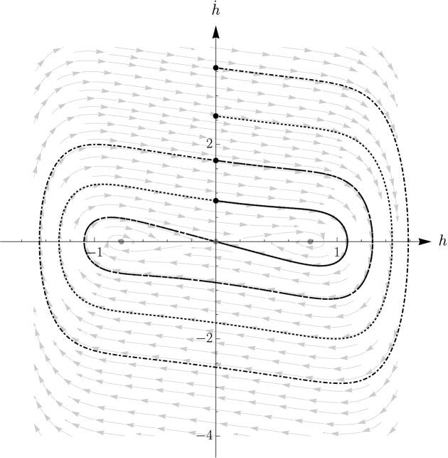
Figure 1. Phase portrait $(h,\dot{h})$ for a sample pair $(d,p)=(3,3)$. The trajectories of the first four static solutions $h_{n}$ ($n=0,1,2,3$) are plotted with distinct line styles and their starting points $(h_{n}(0),\dot{h}_{n}(0))=(0,b_{n})$ are marked with black circles.

$(d,p)$	$(b_{0},c_{0})$	$(b_{1},c_{1})$	$(b_{2},c_{2})$
(3,3)	(0.84261, -4.46847)	(1.67035, -21.7658)	(2.58523, -62.5081)
(3,4)	(1.20653, -3.71646)	(2.48958, -13.0365)	(3.90145, -28.9009)
(3,5)	(1.41849, -3.35818)	(2.95061, -10.1979)	(4.61581, -20.3151)
(5,1)	(5.51059, -22.5426)	(12.4733, -209.872)	(21.5494, -1005.52)
(5,2)	(7.70805, -8.22701)	(18.1434, -32.8788)	(30.9438, -79.2027)
(5,3)	(7.69629, -5.64440)	(17.4958, -17.8598)	(28.8616, -36.3276)

Table 1. Parameters $b_{n}$ and $c_{n}$ of the first three static solutions for a few pairs $(d,p)$.

We remark that no static solutions exist in the critical and subcritical cases $p\leq 2/(d-2)$, as follows, for instance, from the identity

$$\frac{1}{2}\dot{h}^{2}(0)=\left(d-2-\frac{2}{p}\right)\int_{0}^{\infty}\dot{h}^{2}(s)ds\,,$$ (7)

which arises from multiplying equation (5) by $\dot{h}$ and integrating by parts.

The role of static solutions in dynamics depends on their stability properties. To determine the linear stability of the solution $\phi_{n}(r)$, we substitute $\phi(t,r)=\phi_{n}(r)+w(t,r)$ into (2). Dropping nonlinear terms in $w$, we get the linearized equation

$$w_{tt}=w_{rr}+\frac{d-1}{r}w_{r}+(2p+1)\phi_{n}^{2p}w\,.$$ (8)

Substituting $w(t,r)=e^{\lambda t}v(r)$ into (8), we obtain the eigenvalue problem

$$L_{n}v:=\left(-\frac{d^{2}}{dr^{2}}-\frac{d-1}{r}\frac{d}{dr}-(2p+1)\phi^{2p}_{n}(r)\right)v=-\lambda^{2}v.$$ (9)

For each $n$ the operator $L_{n}$ is essentially self-adjoint in the Hilbert space $X=\{v:\int_{1}^{\infty}v^{2}(r)r^{d-1}dr<\infty,\,v(1)=0\}$. Since $\phi_{n}(r)$ is bounded and decays to zero at infinity, $L_{n}$ has a continuous spectrum $[0,\infty)$. Note that the function generated by scaling

$$v_{0}^{(n)}(r)=\Big{.}\frac{d}{d\alpha}\alpha^{1/p}\phi_{n}(\alpha r)\Big{|}_{\alpha=1}=r\phi_{n}^{\prime}(r)+\frac{1}{p}\phi_{n}(r)$$ (10)

solves equation (9) for $\lambda=0$ (but it is not an eigenfunction because it does not belong to $X$). From the phase-plane analysis above it follows that $v_{0}^{(n)}(r)$ has exactly $n$ zeros which implies by the Sturm oscillation argument that the operator $L_{n}$ has exactly $n$ negative eigenvalues, hereafter denoted by $-(\lambda_{k}^{(n)})^{2}$ ($k=1,..,n$). Consequently, the static solution $\phi_{n}$ has exactly $n$ unstable modes $v_{k}^{(n)}(r)e^{\lambda_{k}^{(n)}t}$. In what follows we focus on dynamics near the ground state solution $\phi_{0}(r)$ which has exactly one unstable mode $v_{1}(r)e^{\lambda_{1}t}$ (henceforth we drop the superscript $(n)$ on the eigenvalues and eigenfunctions). Due to the presence of the unstable mode, generic solutions of the linearized equation (8) grow exponentially. This instability can be eliminated by preparing initial data that are orthogonal to the unstable mode. The solutions starting from such special initial data decay in time due to a combination of two dispersive effects: the quasinormal ringdown and the polynomial tail. The rate of decay of the tail is determined by the fall-off of the potential term in (8): since $\phi_{0}^{2p}(r)\sim r^{-2p(d-2)}$ for $r\rightarrow\infty$, it follows that $\phi(t,r)\sim t^{-\beta}$, where $\beta=d-4+2p(d-2)$, for any fixed $r>1$ and $t\rightarrow\infty$ [1, 9]. The ringdown is determined by the quasinormal modes which are solutions of the eigenvalue equation (9) with $\operatorname{Re}(\lambda)<0$ satisfying the outgoing wave condition $v(r)\sim e^{-\lambda r}$ for $r\rightarrow\infty$. As the concept of quasinormal modes is inherently related to the loss of energy by radiation, the unitary evolution (8) and the associated self-adjoint eigenvalue problem (9) do not provide a natural setting for analysing quasinormal modes, both from the conceptual and computational viewpoints. For this reason we postpone the discussion of quasinormal modes until the next section where a new nonunitary formulation will be introduced.

3. Characteristic initial-boundary value formulation

The rest of the paper is devoted to dynamics of convergence to $\phi_{0}$ for initial data fine-tuned to the threshold. To this order we introduce the null coordinate $u=t-r$ and the inverse radial coordinate $x=1/r$ which compactifies the spatial domain to the interval $0\leq x\leq 1$. Then $f(u,x)=r^{\frac{d-1}{2}}\phi(t,r)$ satisfies the equation

$$2f_{ux}+x^{2}f_{xx}+2xf_{x}-\frac{1}{4}(d-3)(d-1)f+x^{\alpha}f^{2p+1}=0,\quad f(u,1)=0,$$ (11)

where $\alpha=\frac{1}{2}(p(d-1)-2)$. We note in passing that equation (11) can be written as the conservation law

$$\partial_{x}\left(f_{u}^{2}+x^{2}f_{u}f_{x}\right)=\partial_{u}\left(\frac{1}{2}x^{2}f_{x}^{2}+\frac{1}{8}(d-3)(d-1)f^{2}-\frac{1}{2p+2}x^{\alpha}f^{2p+2}\right)\,,$$ (12)

which upon integration gives the energy loss formula

$$\frac{dE}{du}=-f_{u}(u,0)^{2},$$ (13)

where

$$E[f]=\int_{0}^{1}\left(\frac{1}{2}x^{2}f_{x}^{2}+\frac{1}{8}(d-3)(d-1)f^{2}-\frac{1}{2p+2}x^{\alpha}f^{2p+2}\right)dx\,.$$ (14)

As follows from section 2, equation (11) has infinitely many static solutions $f_{n}(x)$ which behave as $f_{n}(x)\sim c_{n}x^{\frac{d-3}{2}}$ near $x=0$ and vanish at $x=1$. These static solutions are critical points of the energy functional $E[f]$; in particular, the solution $f_{0}$ is the ground state.

We now repeat the linear stability from the previous section by substituting $f(u,x)=f_{0}(x)+e^{\lambda u}v(x)$ into (11) and linearizing. This yields the eigenvalue problem

$$x^{2}v^{\prime\prime}+2xv^{\prime}+2\lambda v^{\prime}-\frac{1}{4}(d-3)(d-1)v+(2p+1)x^{\alpha}f_{0}^{2p}(x)v=0,\quad\,v(1)=0.$$ (15)

An advantage of this formulation is that it allows us to treat quasinormal modes as genuine eigenfunctions. To do so we must specify the desired behavior of eigenfunctions at $x=0$ which is rather subtle because this endpoint is an essential singularity. The two linearly independent solutions of equation (15) near $x=0$ have the following leading behaviors

$$v_{g}(x)\sim 1,\qquad v_{b}(x)\sim e^{2\lambda/x}\,,$$ (16)

where the subscripts $g$ and $b$ stand for ‘good’ and ‘bad’ solutions, respectively. At $x=0$ the solution $v_{g}(x)$ admits a formal Taylor series, while the solution $v_{b}(x)$ has an essential singularity. In terms of the original variables, these two solutions correspond to the outgoing and ingoing waves, respectively, thus we demand that the eigenfunctions have no admixture of $v_{b}$. Having a good solution near $x=0$, one can shoot it towards $x=1$ and determine the eigenvalues from the boundary condition $v(1)=0$. Since the formal Taylor series of $v_{g}$ is in general divergent, in practice we take the asymptotic expansion of $v_{g}(x)$ at some small $x_{0}$ and truncate it at the least term. While this optimal truncation approach works very well in the case of positive (unstable) eigenvalues, it is not precise enough for the eigenvalues with $\operatorname{Re}(\lambda)<0$ because in this case the bad solution $v_{b}(x)$ is smaller than any power of $x$ for $x\rightarrow 0^{+}$. To capture such a small term we use the Borel summation method which goes as follows. Given a formal power series $v_{g}(x)=\sum_{k=0}^{\infty}a_{k}x^{k}$, we Borel transform it

$$\mathcal{B}(x)=\sum_{k=0}^{\infty}\frac{a_{k}}{k!}x^{k}\,.$$ (17)

and then take the Laplace transform to get the Borel sum

$$\mathcal{B}_{S}(x)=\int_{0}^{+\infty}e^{-t}\mathcal{B}(tx)dt\,.$$ (18)

In practice, we truncate the series in (17) at some high order $2K$ and accelerate the convergence by using the (diagonal) Padé approximation $P_{K}\mathcal{B}$. Because of possible poles of the Padé approximation on the real axis, we deform the integration contour in (18) by introducing the following path on the complex plane $\gamma(\varepsilon)=\gamma_{1}\cup\gamma_{2}$ with

$$\gamma_{1}\,:\ [0,\varepsilon]\ni s\rightarrow is\in\mathbb{C},\quad\gamma_{2}\,:\ [0,\infty)\ni s\rightarrow i\varepsilon+s\in\mathbb{C},$$ (19)

where $\varepsilon$ is a free real parameter (since the integrand decays sufficiently fast we need not to close the contour ‘at infinity’). In our calculations we took the mean of integrals along the contours $\gamma(\varepsilon)$ and $\gamma(-\varepsilon)$, thus we approximated (18) by

$$\mathcal{B}_{S}(x)\approx\frac{1}{2}\int_{\gamma(\varepsilon)}e^{-t}P_{K}\mathcal{B}(tx)dt+\frac{1}{2}\int_{\gamma(-\varepsilon)}e^{-t}P_{K}\mathcal{B}(tx)dr\,.$$ (20)

and then computed these integrals numerically.

Having set up initial conditions at $x_{0}$ (either by the optimal truncation or Borel summation), we integrated Eq. (15) using an adaptive Runge-Kutta method of 8th order and then determined the eigenvalues by solving the boundary condition $v(1)=0$ with Newton’s method (see Tab. 2). To suppress round-off errors we used an extended precision arithmetics, typically with more than $20$ digits. Particularly demanding was the computation of the first stable eigenvalue $\lambda_{2}$ for $d=3$. For example, in the case $(d,p)=(3,3)$ we used $x_{0}\approx 0.00825$, $K=128$, $\varepsilon=10$ and Gauss quadratures with $38$ and $128$ nodes for Gauss-Legendre and Gauss-Laguerre rules to compute the integrals (20) along $\gamma_{1}$ and $\gamma_{2}$ respectively. This scheme provided an accurate enough initial conditions for the shooting algorithm to produce $\lambda_{2}\approx-0.04328358...$ whose first 15 digits did not depend on the choice of the starting point $x_{0}$ which made us feel confident that the result is correct.

$(d,p)$	$\lambda_{1}$	$\lambda_{2}$	$\lambda_{3}$
(3,3)	0.4376132	-0.04328358	-0.7359469 $\pm$ 0.6611351$\,i$
(3,4)	0.9119156	-0.12566311	-0.9112554 $\pm$ 1.228442$\,i$0
(3,5)	1.3939640	-0.21578421	-0.9589717 $\pm$ 1.608909$\,i$0
(5,1)	1.4129620	-0.1580264 $\pm$ 0.2094073$\,i$	-3.6633570 $\pm$ 1.863078$\,i$0
(5,2)	4.0066460	-0.5943277 $\pm$ 0.4789266$\,i$	-5.0621700 $\pm$ 5.850155$\,i$0
(5,3)	6.4729880	-0.9450331 $\pm$ 0.5032462$\,i$	-5.0503320 $\pm$ 8.049461$\,i$0

Table 2. The unstable eigenvalue $\lambda_{1}$ and two least damped stable eigenvalues $\lambda_{2},\lambda_{3}$ of the linearized operator around the ground state solution $f_{0}$ for several pairs $(d,p)$. All given digits are significant.

In the appendix we describe a different method of finding the spectrum of the linearized problem which reproduces all the above eigenvalues except for those that lie on the negative real axis.

4. Critical evolution

In this section we give numerical evidence supporting our conjecture that the ground state solution $f_{0}$ sits at the threshold for generic blowup.

Before presenting results we briefly describe our method of solving numerically the initial-boundary value problem (11). We use the method of lines with a spectral element method for space discretization. The starting point of this approach is a weak formulation of equation (11). The spatial domain is divided into non-overlapping intervals and on each interval the integral is approximated using the Gauss-Legendre quadrature formula. We typically use 16 grid points in each of 9 equal size intervals of the spatial domain. The coupling between the intervals is enforced by the requirement of smoothness. At the sphere $x=1$ we impose the Dirichlet condition, while at null infinity $x=0$ no condition is imposed. The resulting equations are integrated in time using the 6th order Runge-Kutta scheme with a fixed time step. The presence of the mixed derivative in equation (11) required a solution of the algebraic system at the internal steps of the Runge-Kutta scheme.

To get a clear picture of near critical evolution it was instrumental to use high precision arithmetics which is computationally expensive. The numerical algorithm described above gave satisfactory results at an acceptable cost. The efficiency of the spectral element method is due to its fast convergence and the sparse (block diagonal) structure of matrices. To further speed up calculations we use a parallel version of the bisection search to fine tune the initial data. The code was written in Mathematica.

We illustrate our numerical results for a one-parameter family of initial data

$$f(0,x)=a\sin^{2}\left(\pi x\right)e^{-200(x-1/2)^{2}}\,.$$ (21)

which interpolates between dispersion to zero for small amplitudes $a$ and the ODE blowup for large $a$. Using bisection we fine tune the amplitude to the critical value $a_{*}$ separating these two generic behaviors. For such fine-tuned initial data we observe for intermediate times the convergence to the ground state $f_{0}$. This is shown in Fig. 2 for two pairs $(d,p)=(3,3)$ and $(5,2)$.

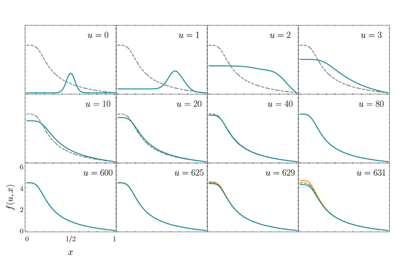
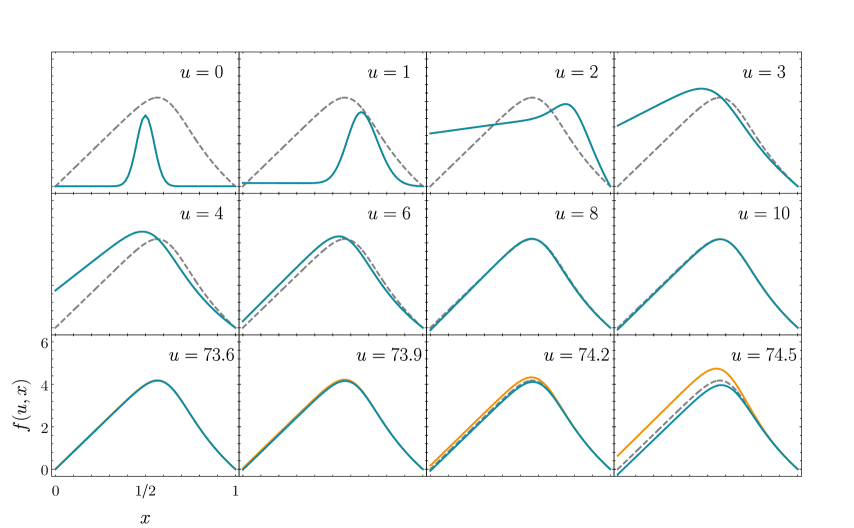
Figure 2. Snapshots of near critical evolution of initial data (21) for $(d,p)=(3,3)$ (upper plot) and $(d,p)=(5,2)$ (lower plot). The amplitudes of marginally subcritical (blue lines) and supercritical (orange lines) data differ by $10^{-128}$. Initially the solutions evolve together, approach $f_{0}$ (dashed lines) for intermediate times, and eventually depart in opposite directions.

For intermediate times, when the nearly critical solution is close to the ground state $f_{0}$, the dynamics is well approximated (for any fixed $x$) by the linearized formula

$$f(u,x)=f_{0}(x)+c_{1}e^{\lambda_{1}u}+\underbrace{\operatorname{Re}\left(c_{2}e^{\lambda_{2}u}\right)+\ldots}_{\text{ringdown}}+\underbrace{c_{3}u^{-\beta}\left(1+\frac{c_{4}}{u}+\frac{c_{5}}{u^{2}}+\ldots\right)}_{\text{tail}}\,,$$ (22)

where $c_{i}$ are ($x$ dependent) parameters and dots denote subleading terms. For exactly critical data the coefficient $c_{1}$ vanishes. Our bisection procedure ensures that $c_{1}\sim a-a_{*}$ is very small, typically of order $10^{-128}$, which gives a reasonably long span of time $\propto-\frac{1}{\lambda_{1}}\log|a-a_{*}|$ over which the linearized approximation (22) is expected to hold and can be fitted to the nearly critical solution shown in Fig. 2. Performing this fit (keeping the exponent of the tail $\beta=d-4+2p(d-2)$ fixed) we reproduce the eigenvalues $\lambda_{1}$ and $\lambda_{2}$ with precision of $0.01\%$ which is very reassuring; see Fig. 3.

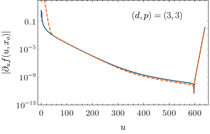
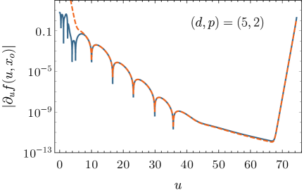
Figure 3. Pointwise convergence to $f_{0}$ at a sample interior point $x_{o}=5/9$ for the same marginally subcritical data as in Fig. 2. The dashed lines depict the fits based on formula (22). For $(d,p)=(5,2)$ the evolution has two well-separated phases: the quasinormal ringdown followed by the polynomial tail. For $(d,p)=(3,3)$ the least damped quasinormal mode is non-oscillatory and very slowly decaying which makes it harder to separate it from the tail.

Appendix A Pseudospectral solution of the linear problem

Here we present a simple algebraic method of solving the linearized characteristic initial-boundary value problem which reproduces most (but not all) results from section 3.

Linearization of equation (11) around a static solution $f_{n}$ yields

$$\partial^{2}_{ux}v=L_{n}v\,,$$ (23)

with

$$L_{n}:=\frac{1}{2}\left(-x^{2}\partial_{x}^{2}-2x\partial_{x}+\frac{1}{4}(d-3)(d-1)-(2p+1)x^{\alpha}f_{n}^{2p}(x)\right)\,.$$ (24)

Discretization in space transforms equation (23) into a system of $N$ coupled constant-coefficient ODEs, where $N$ is the number of degrees of freedom introduced by discretization. In the case at hand, $N$ is the number of Chebyshev polynomials used in the spatial approximation of $v(u,x)$. This semi-discrete problem has the form

$$\mathbf{D}\frac{d}{du}\mathbf{v}=\mathbf{L}_{n}\mathbf{v}\,,$$ (25)

where $\mathbf{v}$ is a vector of unknowns, $\mathbf{D}$ is an invertible discrete version of $\partial_{x}$ which incorporates the boundary condition $v(u,1)=0$, and $\mathbf{L}_{n}$ is a discretization of $L_{n}$. We rewrite (25) as

$$\frac{d}{du}\mathbf{v}=\mathbf{D}^{-1}\mathbf{L}_{n}\mathbf{v}\,,$$ (26)

and performing diagonalization

$$\mathbf{D}^{-1}\mathbf{L}_{n}=\mathbf{P}\Lambda\mathbf{P}^{-1},\quad\Lambda=\mathrm{diag}\left(\Lambda_{1},\ldots,\Lambda_{N}\right)\,,$$ (27)

we solve the system (25) by exponentiation

$$\mathbf{v}(u)=\mathbf{P}\exp\left(\Lambda u\right)\mathbf{P}^{-1}\mathbf{v}(0),$$ (28)

where $\mathbf{v}(0)$ is a vector of initial data. As $N$ grows, the eigenvalues $\Lambda_{i}$, $i=1,\ldots,N$ tend to the eigenvalues $\lambda$ of (15), hence by increasing $N$ we uncover more and more eigenvalues found in section 3 with the shooting method. This is illustrated in Fig. 4. The drawback of this method is the accumulation of spurious eigenvalues on the negative real axis which makes it hardly possible to extract the genuine eigenvalues lying on that axis (such as $\lambda_{2}$ for $d=3$).

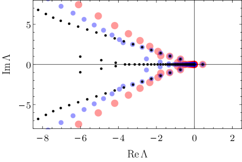
Figure 4. Eigenvalues $\Lambda_{i}$ of the discrete operator $\mathbf{D}^{-1}\mathbf{L}_{0}$ in the $(d,p)=(3,3)$ case for different numbers of Chebyshev polynomials used in the approximation: $N=64$ (red), $N=128$ (blue), $N=256$ (black). As $N$ increases, we observe accumulation of spurious eigenvalues on the negative real axis and convergence to the genuine eigenvalues elsewhere.

Interestingly enough, using a large enough number of polynomials we were able (after removing the unstable mode from the initial data) to see in the evolution the polynomial tail whose exponent is in agreement with [9], cf. Fig. 5.

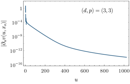
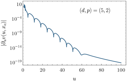
Figure 5. Pointwise decay (at a sample interior point $x_{o}=5/9$) of the linear perturbation of $f_{0}$ as governed by Eq. (23) for $(d,p)=(3,3)$ and $(d,p)=(5,2)$ for sample compactly supported initial data with the unstable mode removed. Numerical solution uses $N=1024$ Chebyshev polynomials, cf. Fig. 3.

References

- [1] W. A. Strauss, K. Tsutaya, Existence and blow up of small amplitude nonlinear waves with a negative potential, Discrete Cont. Dyn. Sys. 3, 175 (1997)
- [2] P. Bizoń, T. Chmaj, Z. Tabor, On blowup for semilinear wave equations with a focusing nonlinearity, Nonlinearity 17, 2187 (2004)
- [3] R. Donninger, Nonlinear stability of self-similar solutions for semilinear wave equations, Communications in Partial Differential Equations 35, 669 (2010)
- [4] P. Bizoń, D. Maison, A. Wasserman, Self-similar solutions of semilinear wave equations, Nonlinearity 20, 2061 (2007)
- [5] R. Donninger, B. Schörkhuber, Stable blow up dynamics for energy supercritical wave equations, Trans. Amer. Math. Soc. 366, 2167 (2014)
- [6] I. Glogić, B. Schörkhuber, Co-dimension one stable blowup for the supercritical cubic wave equation, arXiv:1810.07681
- [7] T. Cazenave, An introduction to semilinear elliptic equations, Editora do IM-UFRJ, Rio de Janeiro, 2006.
- [8] R. H. Fowler, The Solutions of Emden’s and Similar Differential Equations, MNRAS 91, 63 (1930)
- [9] P. Bizoń, T. Chmaj, A. Rostworowski, Anomalously small wave tails in higher dimensions, Phys. Rev. D 76, 124035 (2007)