Functional Asplund metrics for pattern matching, robust to variable lighting conditions
Abstract
In this paper, we propose a complete framework to process images captured under uncontrolled lighting and especially under low lighting. By taking advantage of the Logarithmic Image Processing (LIP) context, we study two novel functional metrics: i) the LIP-multiplicative Asplund metric which is robust to object absorption variations and ii) the LIP-additive Asplund metric which is robust to variations of source intensity or camera exposure-time. We introduce robust to noise versions of these metrics. We demonstrate that the maps of their corresponding distances between an image and a reference template are linked to Mathematical Morphology. This facilitates their implementation. We assess them in various situations with different lightings and movement. Results show that those maps of distances are robust to lighting variations. Importantly, they are efficient to detect patterns in low-contrast images with a template acquired under a different lighting.
keywords:
Asplund metrics, Double-sided probing, Logarithmic Image Processing, Map of Asplund distances, Mathematical Morphology, Pattern matching, Robustness to lighting variations1]University of Strathclyde, Department of Mathematics and Statistics, G11XQ Glasgow, Scotland, United Kingdom 2]International Prevention Research Institute, 69006 Lyon, France 3]Université Jean Monnet, Laboratoire Hubert Curien, UMR CNRS 5516, 42000 Saint-Etienne, France {paper}
1 Introduction
Metrics or their values, namely the distances, play a central role in image analysis as comparison tools. They possess strong mathematical properties (symmetry, separation, triangular inequality) but they are generally not founded on optical properties. They are therefore not adapted to the comparison of images captured under variable lighting conditions. This issue affects most classical metrics like: the Euclidean-like distances (Li and Lu, 2009; Wang et al., 2005), the integral metric, the uniform metric, the Stepanov distance (or Minkowski distance) (Deza and Deza, 2016), the Hausdorff metric (Dougherty, 1991; Huttenlocher et al., 1993) and many others (Deza and Deza, 2016). The aim of this paper is to propose metric tools robust to lighting variations.
Analysing images captured with variable lighting conditions is a challenging task that can occur in many settings, such as traffic control (Messelodi et al., 2005; Salti et al., 2015), safety and surveillance (Foresti et al., 2005), underwater vision (Peng and Cosman, 2017; Ancuti et al., 2018), driving assistance (Hautière et al., 2006), face recognition (Chen et al., 2006; Faraji and Qi, 2016; Hussain Shah et al., 2015; Lai et al., 2014), large public health databases of images (Noyel et al., 2017), etc. There is some data in the literature about the difficulties inherent to this issue. Chen et al. (2006) observe that the performance of classical techniques like gamma correction (Shan et al., 2003), logarithm transform (Savvides and Kumar, 2003), adaptive histogram equalisation (Pizer et al., 1987), region-based histogram equalisation (Shan et al., 2003), and block-based histogram equalisation (Xie and Lam, 2005) present limitations. They propose a Discrete Cosine Transform in the logarithm domain (Chen et al., 2006). Faraji and Qi (2016) suggest other solutions based on logarithmic fractal dimension. Hussain Shah et al. (2015) claim that: “Firstly, textural values are changed during illumination normalisation due to increase in the contrast that changes the original pixels of [images]. Secondly, it minimises the distance between inter-classes which increases the false acceptance rates”. Unsharp masking algorithm (Deng, 2011) or retinex type of algorithms (Meylan and Susstrunk, 2006) do not take into account the enhancement of noise. Consequently, the usual approach which consists of a pre-processing to normalise the illumination, significantly increases the difficulty to perform the second step dedicated to the recognition of a pattern. Moreover, the pre-processing is rarely based on a rigorous modelling of the cause of the lighting variations. We address this issue by proposing metric tools which are efficient in presence of lighting variations, without any pre-processing. Those metrics are especially robust to variations between low-contrast and high-contrast images. We start from a little-known metric defined for binary shapes (Asplund, 1960; Grünbaum, 1963), namely the Asplund metric. It consists of a double-sided probing of one of the shapes by the other. This binary metric has the outstanding property of being insensitive to object magnification (Jourlin et al., 2014). Our motivation has been to extend this property to Asplund-like metrics dedicated to grey level images. Such extensions of the binary Asplund metric to the functional case require the use of homothetic images or functions which are insensitive to lighting variations. Such a concept is mathematically well defined and physically justified in the Logarithmic Image Processing (LIP) framework (Jourlin and Pinoli, 2001; Jourlin, 2016). Two extensions will be studied: i) the LIP-multiplicative Asplund metric based on the LIP-multiplication operation of an image by a real number and ii) the LIP-additive metric based on the LIP-addition operation of an image by a constant. A famous optical law, the Transmittance Law, is at the basis of both LIP-operations (Jourlin, 2016, chap. 1). They give to the functional Asplund metrics a strong physical property: a very low sensitivity to lighting variations, especially for under-lighted images. The LIP-multiplicative Asplund metric is thereby theoretically insensitive to variations of the object absorption (or opacity). The LIP-additive metric is defined to be insensitive to variations of source intensity (or exposure-time). For pattern matching purpose, a map of distances is computed between a template and an image. The closest image patterns to the template correspond to the minimal values of the map. The patterns are then detected by finding the map minima. In this paper, we will demonstrate that the maps of distances are related to the well-established framework of Mathematical Morphology (MM) (Matheron, 1967; Serra, 1982; Heijmans, 1994; Najman and Talbot, 2013). This will facilitate their programming as numerous image analysis software contain these operations. Importantly, for the Asplund metrics, there is no empirical pre-processing normalising the image intensity. Moreover, the consistency of the LIP model with Human Vision (Brailean et al., 1991) allows the Asplund metrics to perform pattern matching as a human eye would do. The link between these metrics and the LIP model opens the way to numerous applications with low-lighting (Jourlin, 2016).
In this paper, our aim is to present a complete framework of pattern matching robust to lighting variations between low-contrast and high-contrast images. In detail, our contribution is two-fold. (1) Firstly, we extend the preliminary works defining the functional metrics and their corresponding maps of distances between a template and an image (Jourlin et al., 2012, 2014; Jourlin, 2016; Noyel and Jourlin, 2017a, b; Noyel, 2019a). Beyond the prior work, we add theoretical work at two stages. a) We better define the robust to noise version of the metrics. b) We demonstrate the link between the maps of distances and the MM operations of dilation and erosion (Serra, 1982). An expression will be given between each map of distances and those MM operations. (2) The second part of our contribution is to perform an extensive experimental validation of the metrics on simulated and on real images. We show that the Asplund metrics are efficient for pattern recognition in images captured with different lightings. This is especially the case for the imaging of moving objects, where the motion blur is avoided by shortening the camera exposure-time with the side effect of darkening the images (Fig. 11).
2 Related works and novelty
2.1 Related Works
Pattern matching methods efficient under variable lighting conditions are seldom studied in the literature. This explains the few references closely related to our work. Nevertheless, we can cite two papers of Barat et al. (2003, 2010). The first one proposes the concept of probing in order to replace one of the following methods. (i) The morphological approach proposed by Banon and Faria (1997). (ii) The extension of the “hit-or-miss” transform (Serra, 1982) to grey-level images introduced by Khosravi and Schafer (1996). (iii) The approach inspired by the computation of Hausdorff distance of Odone et al. (2001). (iv) The “multi-scale tree matching” based on boundary segments presented by Cantoni et al. (1998). In the second paper, Barat et al. introduce the double-sided probing of a grey level function , where a pair of probes locally surrounds the representative surface of . Such a technique detects the possible locations of the searched pattern. However, the probes are arbitrarily chosen and simply translated along the grey scale to remain in contact with the function . These translations, which darken (or brighten) the probes, seem to take into account the lighting variations of the image. However, as they are not physically founded, they do not correctly model any of such variations.
2.2 Novelty of the functional Asplund metrics
The novelty of the functional Asplund metrics is to be theoretically insensitive to lighting variations, with a physical origin. Unlike the related works, the functional Asplund metrics use the LIP-multiplicative and LIP-additive laws to compare a given template to a studied grey level function . Due to the LIP-laws, the template generates itself the pair of probes suited to the values of the function . The arbitrary choice of the probes made by Barat et al. (2010) is therefore avoided in our approach.
3 Theoretical background: From a metric for binary shapes to a metric for grey level images
The Asplund metric originally defined for binary shapes (Asplund, 1960; Grünbaum, 1963), has been extended to grey-level images in the LIP-framework by Jourlin et al. (2012, 2014). In this section, we give background notions about the binary Asplund metric, the LIP model, the Functional Asplund metrics and MM.
3.1 Asplund metric for binary shapes
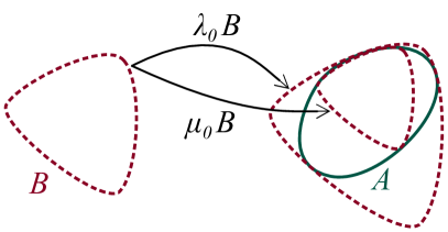
In the initial definition of the Asplund metric for a pair of binary shapes, one shape, e.g. , is chosen to perform the double-sided probing of by means of two homothetic shapes of . Two real numbers are computed: the smallest number such that contains and the greatest number such that contains . The Asplund distance between and is then defined according to:
| (1) |
Remark 1.
This implies that remains unchanged when one shape is magnified or reduced by any ratio .
Fig. 1 illustrates the binary Asplund metric where a shape is probed on its both sides by a reference shape .
The property of insensitivity to object magnification of the binary Asplund metric can be extended to the functional case, where the functional Asplund metric are insensitive to lighting variations. For this purpose, the LIP model is necessary.
3.2 Logarithmic Image Processing
The Logarithmic Image Processing (LIP) model was introduced by Jourlin and Pinoli (1988, 2001). A grey-level image is defined on a domain and takes its values in the grey scale . is an element of the set . Contrary to common usage, the grey scale extremity corresponds to the maximal possible intensity observed by the sensor (white), i.e. when no obstacle is located between the source and the sensor. The other extremity of the scale, , corresponds to the limit case where no element of the source is transmitted (black). For 8-bit digitised images, is equal to 256. Now the two LIP operations on images can be defined: the addition of two images and the scalar multiplication of an image by a real number . Both operations derive from the well-known Transmittance Law (Jourlin, 2016, chap. 1): . The transmittance of a grey level image at a point of is the ratio of the out-coming flux at by the incoming one. The incoming flux corresponds to the source intensity. From a mathematical point of view, the transmittance represents the probability, for a particle of the source arriving in to be seen by the sensor. The Transmittance Law means therefore that the probability of a particle to pass through the addition of two obstacles is nothing but the product of the probabilities to pass through each of them. The transmittance is related to the grey level by the equation . By replacing the transmittances and by their expressions in the one of , the LIP-addition of two images is obtained
| (2) |
Considering that the addition may be written as according to Eq. 2, the multiplication of an image by a real number is then expressed as:
| (3) |
Remark 2.
The opposite function of is easily obtained thanks to the equality , as well as the difference between two grey level functions and :
| (12) | ||||
| (21) |
Let us note that is not an image (as it takes negative values) and is an image if and only if .
The LIP framework possesses the fundamental properties that are listed hereinafter.
Property 1 (The LIP framework is not limited to images in transmission).
As the LIP model is consistent with Human Vision (Brailean et al., 1991), the LIP operators are also valid for images acquired in reflected light. They simulate the interpretation of images by a human eye.
Property 2 (Strong physical properties).
For images acquired in transmission, the LIP-addition (or subtraction) of a constant to (or from) an image consists of adding (or subtracting) a uniform half-transparent object of grey level , which results in a darkening (or lightening) of . Such operations are useful to correct illuminations variations. The images acquired in transmitted or reflected light have both following properties.
- •
-
•
The scalar multiplication of by a positive real number signifies that the thickness (or the absorption) of the half-transparent object which generates is LIP-multiplied by . The image is darkened if or lightened if .
Property 3 (Strong mathematical properties).
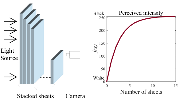
In Fig. 2, several half-transparent sheets are stacked upon each other between a light source and a camera (Mayet et al., 1996; Jourlin, 2016). The camera acquires an image of the light source through the sheets. The perceived intensity by the camera, at a point , is plotted as a function of the number of sheets. The inverted grey scale is used for the intensity axis. When there is no obstacle, the intensity is 0 (white). With the number of stacked sheets, it increases in a logarithmic way and reaches a maximum (black), when no light is perceived trough the sheets. The non-linearity of the perceived intensity is taken into account by the LIP model. Such a model will be useful to define functional Asplund metrics with strong properties.
Remark 3.
There exists a symmetric version of the LIP, namely the Symmetric LIP (Navarro et al., 2013). However, this model is not physically justified albeit it is interesting from a mathematical point of view for its symmetry. It allows e.g. to propose a LIP version of the Laplacian operator or to create Logarithmic Wavelets (Navarro et al., 2014).
3.3 Definition of Functional Asplund metrics
In this section, we will remind the LIP-multiplicative Asplund metric. We will then clarify the definition and properties of the LIP-additive metric.
3.3.1 LIP-multiplicative Asplund metric
Here, we will give the definition of the metric, one of its properties and a rigorous definition. Those were introduced by Jourlin et al. (2012, 2014); Noyel and Jourlin (2017a). Let be the grey-level axis without the zero value and the space of images with strictly positive values.
Definition 1 (LIP-multiplicative Asplund metric).
Let and be two grey level images. As for binary shapes, we select a probing function, e.g. , and we define the two numbers: and . The LIP-multiplicative Asplund metric is defined by:
| (22) |
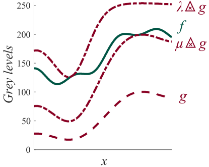
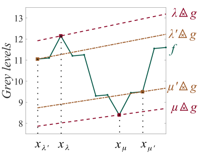
Fig. 3 illustrates the double-sided probing of image by a probe . The lower probe is in contact with the lower side of the function whereas the upper probe is in contact with the upper side of . By comparison with the probe shape, the shapes of the lower and upper probes are deformed by the LIP-multiplication . Such a deformation which depends on the grey value of , is characteristic of the following metric property.
Property 4 (Invariance under LIP-multiplication of a constant).
The strongest advantage of the LIP-multiplicative Asplund metric is to remain unchanged when one image (e.g. ) is replaced by any homothetic , : .
This latest equation demonstrates the insensitivity of the metric to illumination variations modelled by the LIP-multiplicative law , i.e. those which correspond to an absorption change of the object.
Remark 4 (Mathematical appendix (Jourlin, 2016, chap. 3)).
Considering the previous property, it would be more rigorous to explain the LIP-multiplicative Asplund metric as follows.
-
a)
An equivalence relation is defined on the space of grey level images. Two images and are said to be in relation if they satisfy: . The previous relation obviously satisfies the properties of an equivalence relation (reflexivity, symmetry and transitivity).
-
b)
To each image , its equivalence class is associated: .
-
c)
A rigorous definition of the LIP-multiplicative Asplund metric is then given into the space of equivalence classes by: ,
. is the Asplund distance between any elements and of the equivalence classes and .
3.3.2 LIP-additive Asplund metric
As for the LIP-multiplicative metric, we will give a definition of the LIP-additive Asplund metric, some properties and a rigorous definition.
Definition 2 (LIP-additive Asplund metric).
Let and be two functions, we select a probing function, e.g. , and we define the two numbers: and , where lies in the interval . The LIP-additive Asplund metric is defined according to:
| (23) |
Remark 5.
By definition, the values of and lie in the interval , which implies that the probing functions and are not always images. However, is always greater than . Nevertheless, the Asplund metric has the following property.
Proposition 1.
lies in (Proof p. A.1).
Property 5 (Invariance under LIP-addition of a constant).
The LIP-additive Asplund metric remains unchanged when (or ) is replaced by any translated function , with . Indeed, the constants and become and respectively. This implies that and that . Knowing that the addition of a constant to a function is equivalent to a variation of camera exposure-time (Carre and Jourlin, 2014; Deshayes et al., 2015), we have the fundamental result: the LIP-additive Asplund metric is insensitive to exposure-time changing.
Remark 6 (Mathematical appendix).
As for the LIP-multiplicative Asplund metric a rigorous mathematical definition is obtained by replacing each image by its equivalence class , which represents the set of functions such that , for a constant lying in . Nevertheless, if we keep the notation and , there is no ambiguity. Indeed, for a couple of equivalence classes, we have , where and are elements of the classes and respectively.
3.4 Fundamental operations in Mathematical Morphology
As the definitions of the functional Asplund metrics are based on extrema between functions, there exists a natural link with MM as shown by Noyel and Jourlin (2017a). MM (Matheron, 1967; Serra, 1982; Heijmans and Ronse, 1990; Soille, 2004; Bouaynaya and Schonfeld, 2008; Najman and Talbot, 2013; van de Gronde and Roerdink, 2014) is defined in complete lattices (Serra, 1982; Banon and Barrera, 1993). Let us recall some important definitions.
Definition 3 (Complete lattice).
Given a set and a partial order on , is a complete lattice if every subset of has an infimum (a greatest lower bound) and a supremum (a least upper bound).
The infimum and the supremum of will be denoted by and , respectively. Two elements of the complete lattice are important: the least element and the greatest element . E.g. the set of images from to , , is a complete lattice with the partial order relation . The least and greatest elements are the constant functions and whose values are equal to and , respectively, for all the elements of . The supremum and infimum are defined by taking the pointwise infimum and supremum, respectively. For , we have and . Given , the set of functions is also a complete lattice with the usual order .
Definition 4 (Erosion, dilation (Banon and Barrera, 1993)).
Given and two complete lattices, a mapping is
-
•
an erosion : iff , ;
-
•
a dilation : iff , .
As the definitions of these mappings apply even to the empty subset of , we have: and .
A structuring function is a function defined on the domain with its values in , or in . In the case of a dilation or an erosion of a function by an additive structuring function , which is invariant under translation in the domain , the previously defined dilation or erosion can be expressed in the same lattice , or (Serra, 1988; Heijmans and Ronse, 1990) by:
| (24) | ||||
| (25) |
The symbols and represent the extension to functions (Serra, 1982) of Minkowski operations between sets (Serra, 1982). The term “additive structuring function” refers to a vertical translation in the image space (Heijmans and Ronse, 1990).
4 Pattern analysis with the LIP-multiplicative Asplund metric
The LIP-multiplicative Asplund metric is of utmost importance for pattern matching of objects whose absorption (or opacity) is varying. For this purpose, Jourlin et al. (2012) introduced a map of LIP-multiplicative Asplund distances. Noyel and Jourlin (2015) studied it and Noyel and Jourlin (2017a, b)established its link with MM through different conference papers. In this section, we will recall its definition, we will improve the definition of its robust to noise version and we will clearly present the link with MM.

4.1 Map of Asplund distances
Let , be grey-level axes and , the space of strictly positive images.
Definition 5 (Map of LIP-multiplicative Asplund distances (Jourlin et al., 2012)).
Let be a grey-level image and a probe. The map of Asplund distances is defined by:
| (42) |
For each point , the distance is computed in the neighbourhood centred in and the template is acting like a structuring element. is the restriction of to . is the map of Asplund distances between the image and the probe .
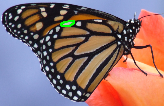
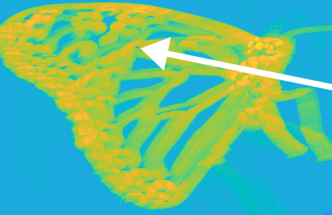
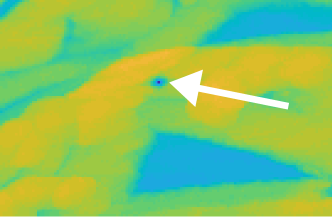
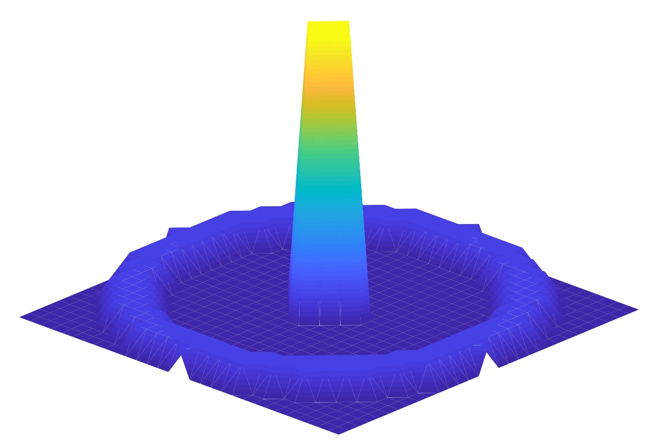
Fig. 4 illustrates the map of Asplund distances with an image of a butterfly (Butterfly, 2010). The image is coming from the Yahoo Flickr Creative Commons 100 Million Dataset (Thomee et al., 2016). The processing is performed on its luminance image which is in grey levels even if the images are displayed in colours. In the luminance image of the butterfly (Fig. 4a), a white spot is selected to serve as a probe (Fig. 4b). The map of Asplund distances between the image and the probe (Fig. 4c) presents a minimum which corresponds to the probe we are looking for (Fig. 4d). A map of Asplund distances allows us therefore to find a reference pattern or probe within an image. However, as images may present acquisition noise, a robust to noise version of the metric is useful for pattern matching.
4.2 A robust to noise version
The Asplund metric is computed using extrema, which makes it sensitive to noise. To overcome this limitation, Jourlin et al. (2014) have proposed an extension which removes from the most penalising points. This idea is related to the topology of the measure convergence (Bourbaki, 2007, chap. 4) in the context of grey-level images. As the image is digitised, the number of pixels lying in is finite. The “measure” of a subset of is linked to the cardinal of this subset, e.g. the percentage of its elements related to the domain (or a region of interest ).
We are looking for a subset of , such that and are neighbours (for the Asplund metric) and the complementary set of related to is small-sized as compared to . This last condition is written: , where represents an acceptable percentage and the number of elements in . A neighbourhood of the image can be defined thanks to a small positive real number as:
| (43) |
The set corresponds to the noise pixels to be discarded. As these pixels are the closest to the probe, they are selected by a function characterising the (LIP-multiplicative) contrast between the functions and and which is defined by:
| (60) | ||||
| (69) |
is the real value by which each image value is LIP-multiplied to be equal to the probe value . The expressions of the probes and (Def. 22) can be written with the contrast function as follows: and . This explains that the closest image values to the upper probe , or the lower probe , correspond to the greatest, or smallest, values of , respectively. Using this property, new probes , or , can be defined on the domain obtained by discarding a percentage of the pixels with the greatest, or smallest, contrast values , respectively. The restricted domain has thereby a cardinal equal to a percentage of the cardinal of .
Definition 6 (LIP-multiplicative Asplund metric with tolerance).
Let be a percentage of points of to be discarded and the set of these discarded points. The (LIP-multiplicative) Asplund metric with tolerance between two grey-level images and is defined by:
| (78) |
The factors and are equal to and. A percentage of the points with the greatest, respectively lowest, contrast values are discarded.
Using Eq. 69 and 3, the contrast function is proportional to the contrast function between the image and the LIP-multiplied probe : , with . This leads to the following property which is demonstrated in the supplementary materials.
Property 6.
The metric is invariant under LIP-multiplication by a scalar.
Remark 7.
A map of Asplund distances with tolerance can be defined as in definition 5: .
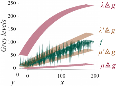
Fig. 5a illustrates the ability of the Asplund metric with tolerance to discard the extremal values and associated to noise. In Fig. 5b, the probe is chosen as a plane and the image is obtained by adding a noise to the probe with a spatial density of . The plane of the probe is distorted by the LIP-multiplication used for the upper probe and for the lower probe . The Asplund distance which is initially equal to decreases to , with a tolerance of . Experiments have shown that with (), the Asplund distance is equal to zero.
4.3 Link with Mathematical Morpho-logy
We first present the maps of distances with neighbourhood operations. We then establish the link with MM in the specific case of a flat structuring element and in the general case of a structuring function.
4.3.1 General expression of the map of Asplund distances with neighbourhood operations
From Eq. 22, for each , there is with and . These expressions show that the map of Asplund distances consists of a double-sided probing, at each point , by the least upper bound and by the greatest lower bound . As and exist for all , the following maps can be defined (Noyel and Jourlin, 2017a).
Definition 7 (LIP-multiplicative maps of the least upper and of the greatest lower bounds (Noyel and Jourlin, 2017a)).
Given , let be an image and a probe. Their map of the least upper bounds (mlub) and their map of the greatest lower bounds (mglb) are defined by:
| (87) | ||||
| (96) |
Let us define , and introduce the general expression of the mlub and of the mglb. Propositions 2 to 4 are demonstrated in (Noyel and Jourlin, 2017a) and in the supplementary materials. Proposition 5 is demonstrated in the Appendix.
Proposition 2.
The mlub and mglb are equal to:
| (97) | ||||
| (98) |
Corollary 1.
Given , , the map of LIP-multiplicative Asplund distances becomes:
| (107) |
4.3.2 Particular case of a flat structuring element
In the case of a flat structuring element, the expressions of the different maps can be simplified as follows.
Proposition 3.
Let be a flat structuring element (, ). The mlub , the mglb and the map of Asplund distances are equal to:
| (108) | ||||
| (109) | ||||
| (118) |
is the reflected (or transposed) domain of the structuring element.
This result shows that the map of Asplund distances is a combination of logarithms, an erosion and a dilation of the image by the flat structuring element . As numerous image processing libraries include erosion and dilation operations, the program implementation becomes easier.
4.3.3 General case: a structuring function
Proposition 4.
The mlub and the mglb are a dilation and an erosion, respectively, between the two complete lattices and .
Let us determine the expressions of this dilation and this erosion using MM with multiplicative structuring functions introduced by Heijmans and Ronse (1990); Heijmans (1994).
Definition 8 (Erosion and dilation with a multiplicative structuring function (Heijmans and Ronse, 1990; Heijmans, 1994)).
Given a function , and a multiplicative structuring function:
| (119) |
is a dilation and
| (120) |
is an erosion, with the convention that when or and that when or . The symbols and represent the extension to multiplicative structuring functions of Minkowski operations between sets (Serra, 1982).
There exists a relation between the multiplicative erosion or dilation and the additive operations of section 3.4 (Heijmans and Ronse, 1990; Heijmans, 1994):
| (121) | ||||
| (122) |
The next proposition gives the morphological expressions of the different maps.
Proposition 5.
Let and , the expressions of the mlub , which is a dilation, and of the mglb , which is an erosion, are:
| (123) | |||||
| (124) |
is the reflected structuring function defined by , (Soille, 2004) and is the function , with . is a transform of .
The map of Asplund distances is the difference between a dilation and an erosion whose expression is:
| (133) |
We notice that the map of LIP-multiplicative Asplund distances is similar to the norm of the morphological gradient also named Beucher’s gradient (Serra, 1988; Soille, 2004). It is the difference between a dilation and an erosion of the transformed image by a structuring function : . This similarity shows that the map of Asplund distances acts as an operator of derivation.
Remark 8.
The map of Asplund distances with tolerance can be computed by replacing the dilation and erosion by rank-filters (Serra, 1988).
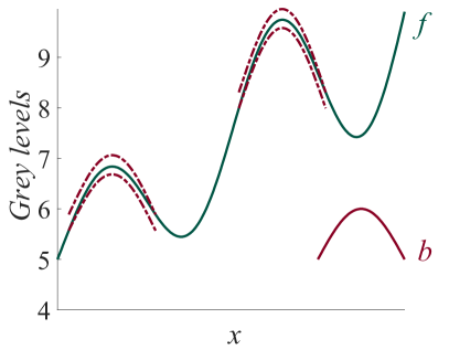
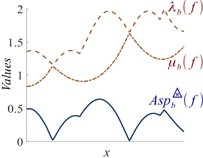
Fig. 6a illustrates the double-sided probing of an image by a probe using the LIP-multiplicative law which modifies the amplitude of the upper probes and of the lower probes . Both peaks have a different amplitude caused by a lighting drift created with the LIP-multiplicative law. In Fig. 6b, when the probe is similar to a pattern in (according to the Asplund distance), the map of Asplund distances of , , presents a local minimum. Here, both peaks are located at the deepest minima of the map of by the probe , . This result shows that the map of LIP-multiplicative Asplund distances is insensitive to a lighting drift corresponding to a variation of absorption (or opacity) of the object.
5 Pattern analysis with the LIP-additive Asplund-like metric
The LIP-additive Asplund metric is useful for images acquired with a small source intensity or a short exposure-time (Jourlin, 2016, chap. 3). In this section, we will introduce: a map of LIP-additive Asplund distances, a robust to noise version of the metric and the link between the map of distances and MM. Due to the important similarity with the LIP-multiplicative case (see previous section), we will only point out the new equations and results. We will consider the set of functions (or ) with values in (or ).
5.1 Map of Asplund distances
Definition 9 (Map of LIP-additive Asplund distances).
Let be a function and a probe. The map of Asplund distances is the mapping defined by:
| (150) |
The LIP addition makes the map of distances robust to contrast variations due to exposure-time changes.
5.2 A robust to noise version
In order to overcome the noise sensitivity of Asplund metric, a neighbourhood of the function is defined by replacing in Eq. 43 the LIP-multiplicative Asplund metric by the LIP-additive one . The noise pixels which are the closest to the probe are selected by using a function which characterises the (LIP-additive) contrast between the functions and :
| (183) |
is the real value to be LIP-added to each function value so that it becomes equal to the probe value . The expressions of the probes and (Def. 23) are equal to: and . These probes are used to introduce the following definition.
Definition 10 (LIP-additive Asplund metric with tolerance).
Let be a percentage of points of to be discarded and the set of these discarded points. The LIP-additive Asplund metric with tolerance between two functions and is defined by:
| (200) |
The constants and are equal to: and. A percentage of the points with the greatest, respectively lowest contrast values are discarded.
From Eq. 183 and 21, the contrast function is related to the contrast function , between and the probe , where , by the following equation: . This leads to the following property demonstrated in the supplementary materials.
Property 7.
The metric is invariant under the LIP-addition of a constant.
Remark 9.
A map of Asplund distances with tolerance can be introduced as in definition 9:.
Fig. 7 illustrates the LIP-additive Asplund metric robust to noise . The probe is chosen as a plane and the function is obtained by adding a noise to the probe with a spatial density of . We notice that the upper probe and the lower probe may take negative values. After the LIP-addition, the planar surface of the probe is still a plane, with a different orientation. The Asplund distance which is initially equal to decreases to , with a tolerance . Experiments have shown that with (), the Asplund distance is equal to zero.
5.3 Link with Mathematical Morpho-logy
5.3.1 General expression for the map of Asplund distances with operations on neighbourhoods
In order to establish the link with MM, we will express the map of Asplund distances with neighbourhood operations. From Eq. 23, for each , the map expression becomes , where and . This leads to the following definition.
Definition 11 (LIP-additive maps of the least upper and of the greatest lower bounds).
Let be a function and a probe. Their map of the least upper bounds (mlub) and their map of the greatest lower bounds (mglb) are defined by:
| (209) | ||||
| (218) |
The following propositions, 6 to 9, are demonstrated in the Appendix. The general expressions of the mlub, mglb and map of distances will be given hereinafter.
Proposition 6.
The mlub and the mglb are equal to
| (227) | ||||
| (236) |
Corollary 2.
The map of Asplund distances between the function and the probe is equal to
| (253) |
5.3.2 Particular case of a flat structuring element
Proposition 7.
Let be a flat structuring element (, ). The mlub , mglb and map of Asplund distances are equal to:
| (262) | ||||
| (271) | ||||
| (288) |
With a flat probe , the map of Asplund distances is a LIP difference between a dilation and an erosion of the function by the domain of the structuring element . It is similar to a morphological gradient with a LIP difference.
5.3.3 General case of a structuring function
Proposition 8.
The mlub (resp. mglb ) is a dilation (resp. an erosion) in the same lattice.
Remark 10.
In Eq. 253, one notices that the map of LIP-additive Asplund distances is a LIP-difference between a dilation and an erosion, which corresponds to the LIP version of the morphological gradient. This similarity shows that the map of Asplund distances acts as an operator of derivation.
Let us establish the relation of the dilation or the erosion with the dilation (Eq. 24) or the erosion (Eq. 25), respectively. For this purpose, a bijective mapping (i.e. an isomorphism) is needed between the lattice of , or , and the lattice of , or . Jourlin and Pinoli (1995); Navarro et al. (2013) defined this isomorphism and its inverse by:
| (289) | ||||
| (290) |
Remark 11.
As and are increasing bijections, they distribute over infima, as well as over suprema.
Proposition 9.
Given two functions , has the property to transform the LIP-difference, , into the usual difference, , .
The dilation (Eq. 227) and the erosion (Eq. 236) can therefore be expressed as:
| (299) | ||||
| (300) | ||||
| (301) |
where .
Proposition 10.
Let be a structuring function and be a function. The expressions of their mlub , which is a dilation, and of their mglb , which is an erosion, are equal to:
| (302) | ||||
| (303) |
is a function defined by .
Their map of Asplund distances is related to the difference between a dilation and an erosion (with an additive structuring function) by:
| (312) | ||||
| (313) |
Remark 12.
By replacing the dilation and erosion by rank-filters (Serra, 1988) one can compute the map of Asplund distances with a tolerance .
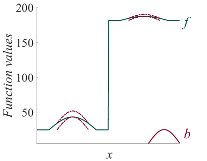
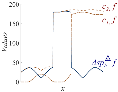
Fig. 8a illustrates the double-sided probing of an image by a probe (or structuring function) . The amplitudes of both peaks are related by a LIP-addition of a constant. In Fig. 8b, the two deepest minima of the map of distances of , correspond to the location of both peaks similar to the probe . This illustrates the insensitivity of the map of LIP-additive Asplund distances to a variation of light intensity or exposure-time.
6 Experiments and results
In this section, we will discuss the implementation of the maps of distances and we will illustrate them with simulated and real cases of image acquisition.
6.1 Implementation
The maps of LIP-multiplicative and LIP-additive Asplund distances of the image , and , respectively, were both programmed in MATLAB® using their direct (Eq. 42, 150) and morphological (Eq. 133, 313) expressions. The same programming was done for the map of Asplund distances with tolerance and of . Due to the existence in numerous image analysis software (e.g. MATLAB®, Python scikit-images) of fast versions of the morphological operations and and of rank filters, the morphological implementation is easier and faster than the direct one. In table 1, the duration of the morphological and of the direct implementations (with parallelisation) of the maps of Asplund distances without and with tolerance are compared using the example of Fig. 9. The image size is of 1224 918 pixels and the probe contains 285 pixels (Fig. 9d). The morphological implementation is always faster than the direct one, with a gain factor lying between 5.9 and 11 (processor Intel® CoreTM i7 CPU 4702HQ, 2.20 GHz, 4 cores, 8 threads with 16 Gb RAM).
| Morpho. | 1.4 s | 4.2 s | 1.4 s | 4.3 s |
| Direct | 16.1 s | 24.6 s | 15.4 s | 25.5 s |
| Gain factor | 10.9 | 5.9 | 11.0 | 5.9 |
6.2 Simulated cases
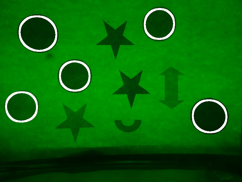
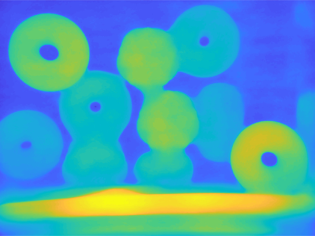
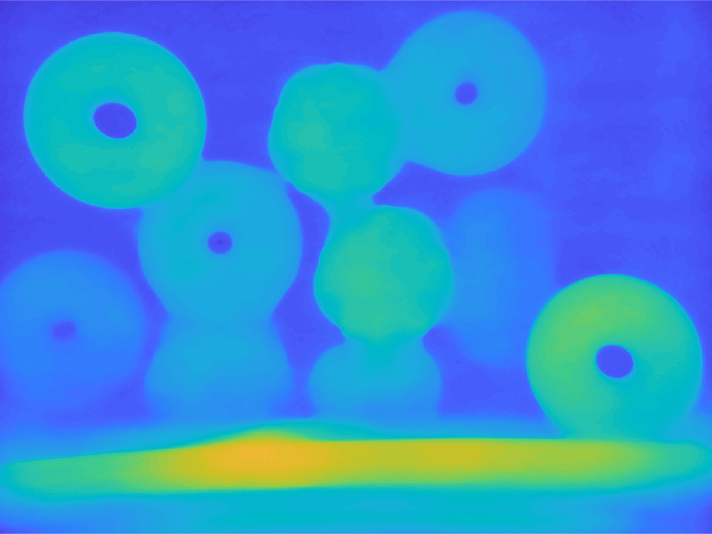
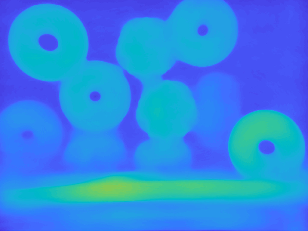
We evaluate the LIP-multiplicative and LIP-additive maps to detect balls in a bright image and in two darkened versions obtained by simulation (Fig. 9). The bright image is acquired in colour with “normal” contrasts – automatically selected by the camera (Fig. 9a) – and converted to a luminance image in grey-level, denoted . A first darkened version is obtained by the LIP-multiplication of by a scalar (Fig. 9b). A second darkened version is obtained by the LIP-addition of a constant (Fig. 9e). Due to the light reflection at the surface of the balls and of other confounding objects, detecting the balls is a difficult task in these images. For this purpose, we used a probe made of a ring surrounding a cylinder (Fig. 9d). The ring has an external radius of 15 pixels, a width of 3 pixels, a grey-level value of 18 and the disk has a radius of 2 pixels and a grey-level value of 190.
Remark 13.
As the grey-scale is complemented in the LIP model, the LIP-multiplicative map is computed using the image complement, and the probe complement . However, the image , darkened by the LIP-addition of a constant, presents negative values and its complement is outside of the dynamic range allowed for the map . For this reason, the darkened image is not complemented.
In the image (Fig. 9a) and in its darkened version (Fig. 9b) obtained by LIP-multiplication, all the balls are detected by a thresholding of their map of Asplund distances (Fig. 9c). The map is the same for both images and because of its invariance under LIP-multiplication by a scalar. Similar results are obtained for the image (Fig. 9a), its darkened version by LIP-addition (Fig. 9e) and their map of distances (Fig. 9f) which is invariant under LIP-addition of a constant. The same parameters of the probe were used for all the images , and . These results show that the maps of Asplund distances are able to detect targets under different illumination conditions modelled by the LIP-multiplication or the LIP-addition .
6.3 Real cases
The maps of LIP-additive and LIP-multiplicative Asplund distances are then illustrated on real images. For a better visual interpretation, the results are presented with colour images even if the processing is made using their luminance.
6.3.1 LIP-additive metric: images acquired with a variable exposure-time
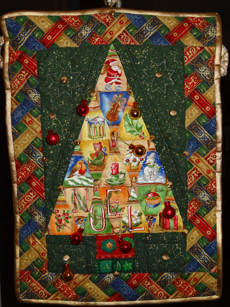
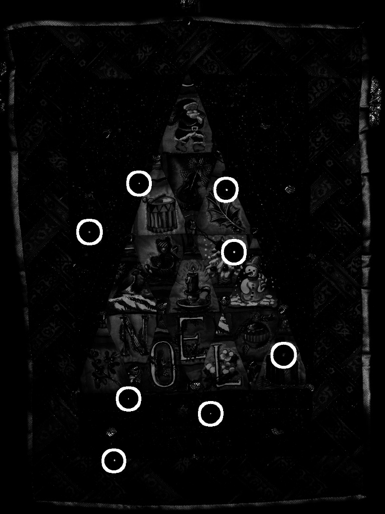
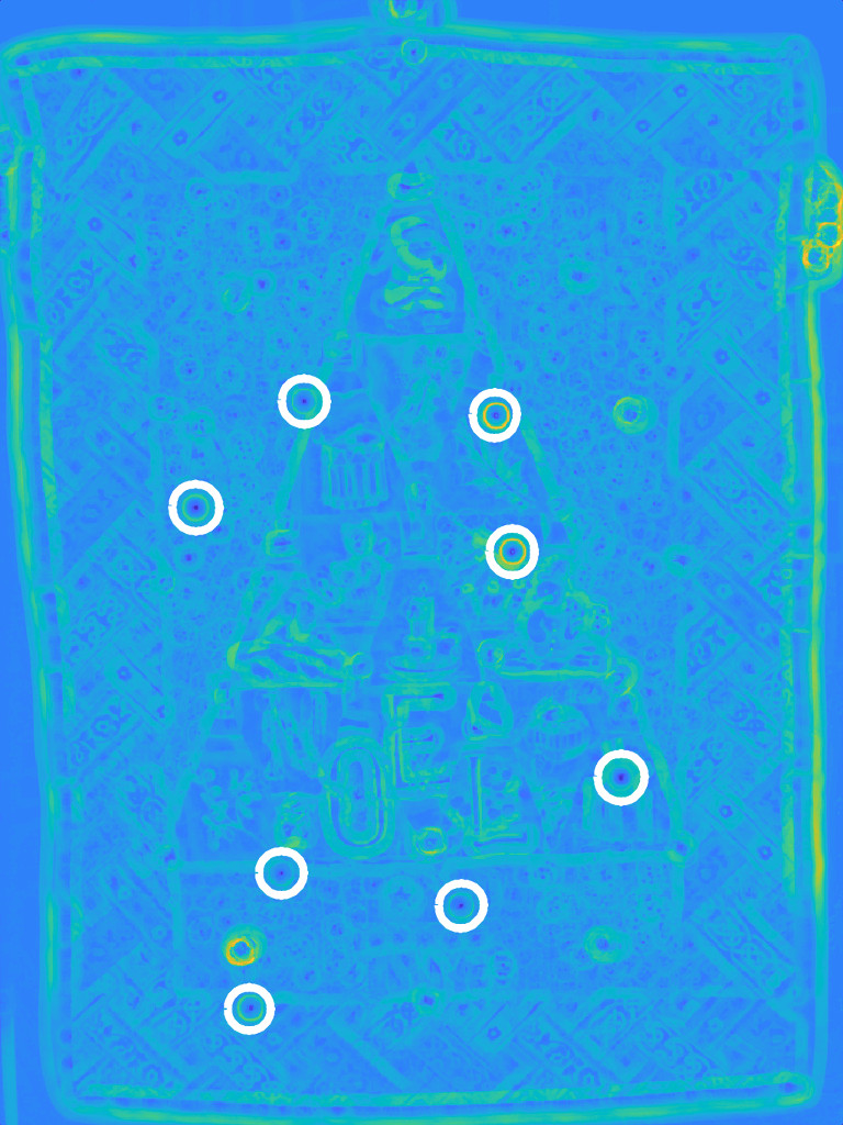
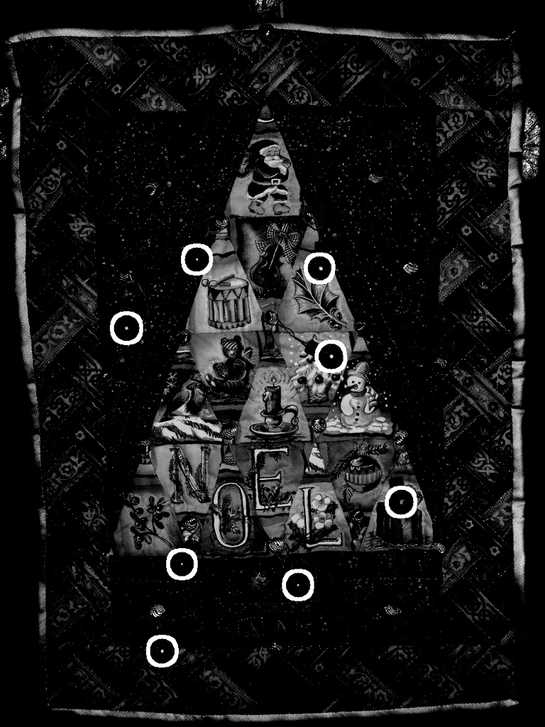
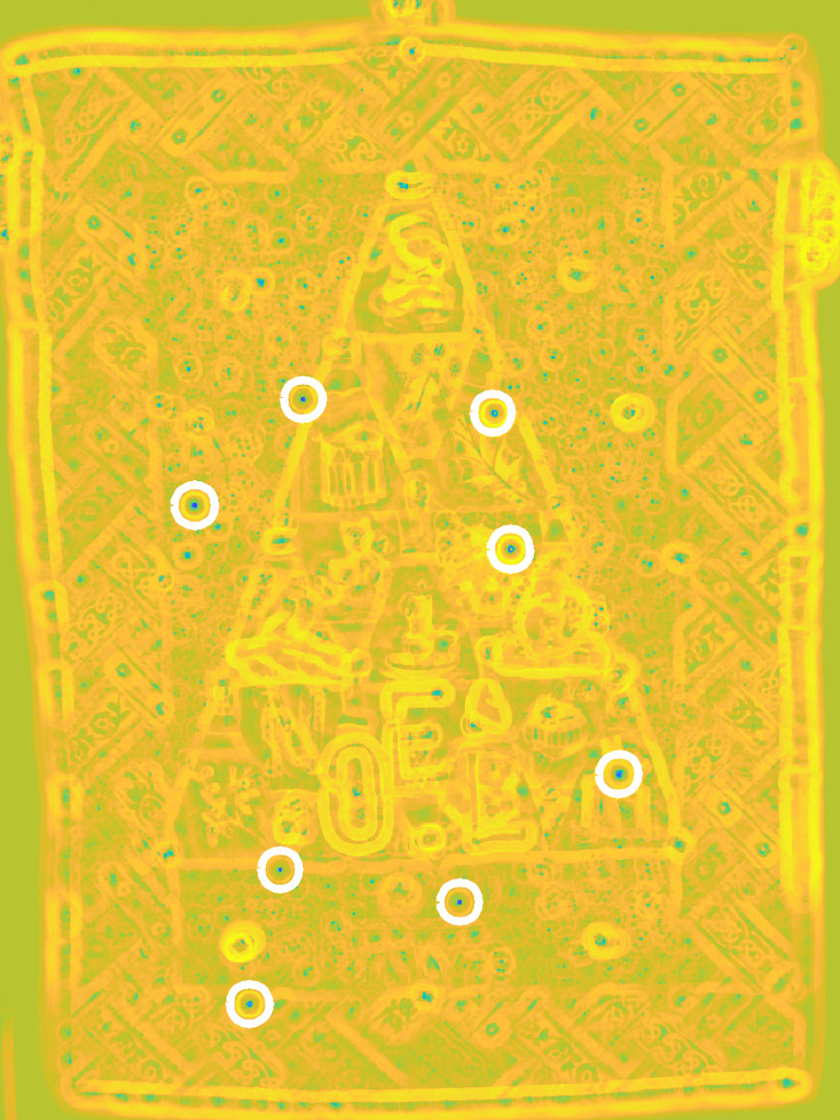
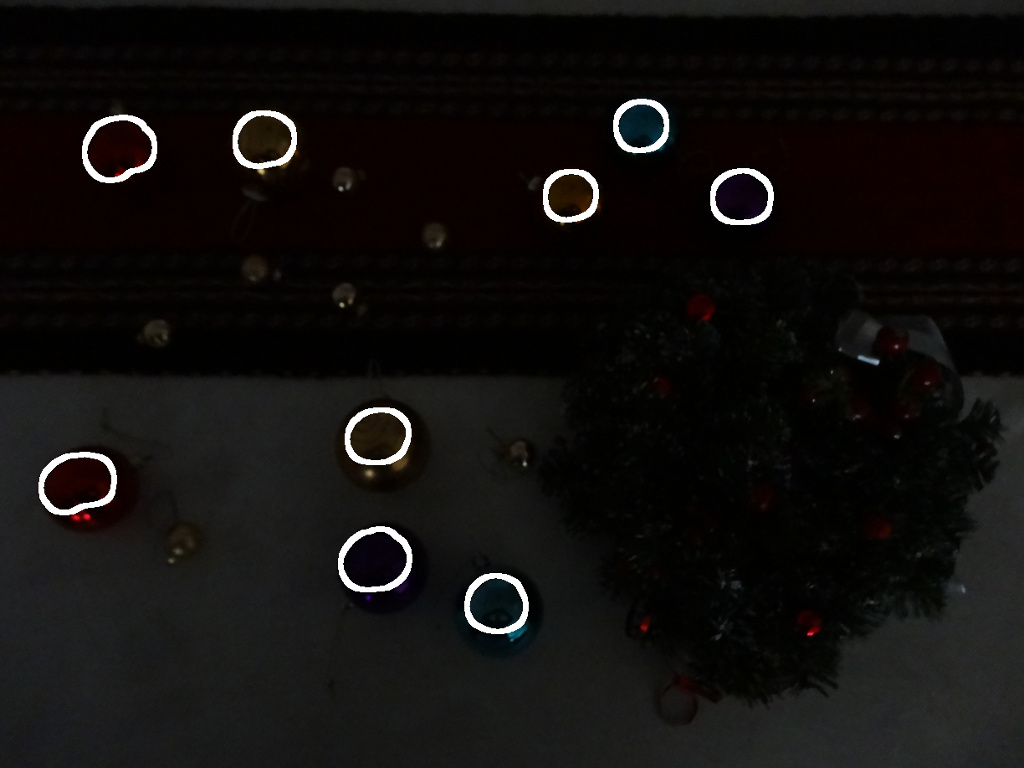
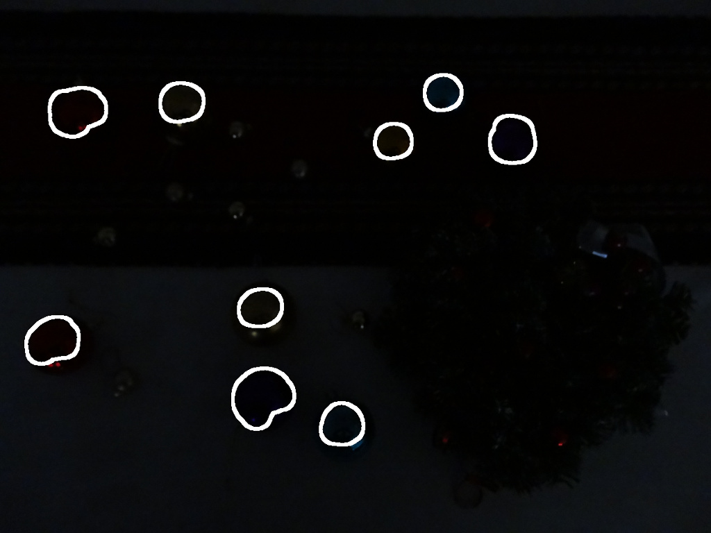
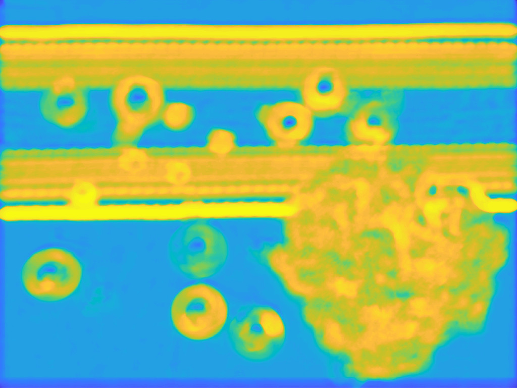
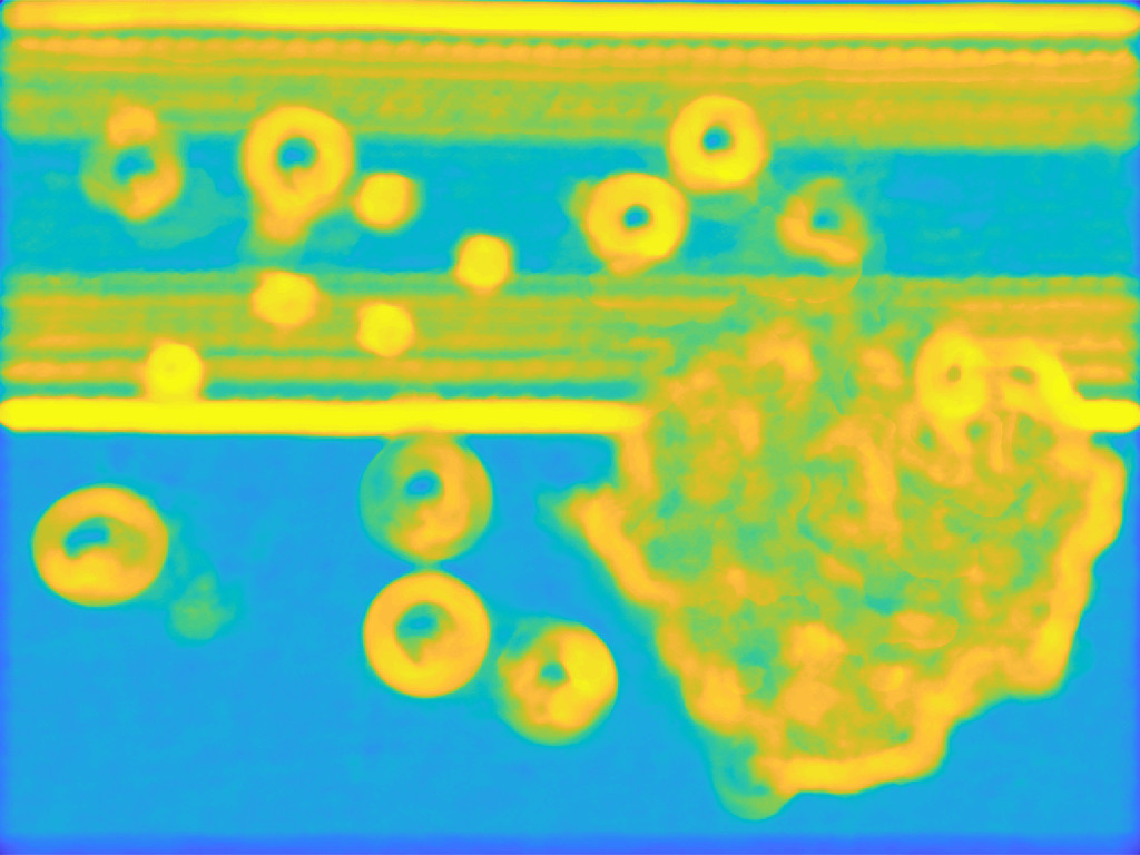
In Fig. 10, the same scene is captured with three different camera exposure-times (or shutter speeds). This gives three images, each with a different brightness: a bright one (Fig. 10a), a dark intermediate one (Fig. 10b) and a dark one (Fig. 10c). The scene is composed of bright balls on a multicolour background with other smaller balls acting as confounding objects. In order to make the ball detection more arduous, the camera is not exactly in the same position to capture the images. Moreover, the balls are of different colours, with different backgrounds and present several reflections. A disk of diameter 55 pixels is manually selected inside a ball of the bright image (Fig. 10a) in order to serve as a probe function . A map of Asplund distances is computed between the complement of each of the three images and the same probe using the same tolerance parameter . In the three distance maps of images (Fig. 10d), (Fig. 10e) and (Fig. 10f), one can notice that the amplitudes are similar. This is caused by the low sensitivity of the LIP-additive Asplund metric to lighting variations due to different exposure-times. In order to extract the location of the large balls, the maps of the dark intermediate image and of the dark image are segmented using the same technique – a threshold (at the percentile) and a reconstruction of the regional h-minima (Soille, 2004) – followed by a morphological post-processing (see remark in supplementary materials). Such a technique allows to detect all the large balls in both dark images (Fig. 10b) and (Fig. 10c), using the same probe extracted in the bright image (Fig. 10a). This illustrates the robustness of the map of LIP-additive Asplund distances to different exposure-times.
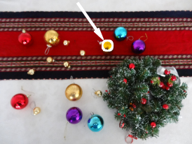
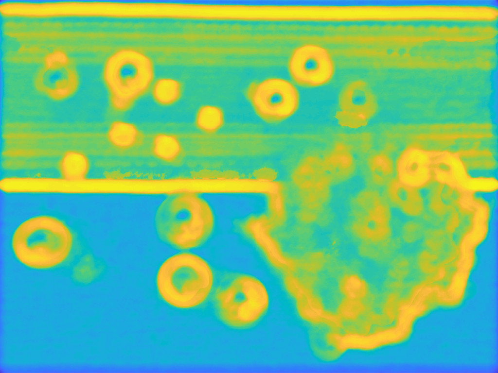
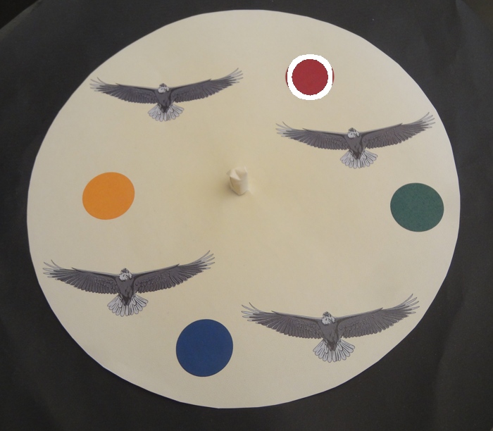
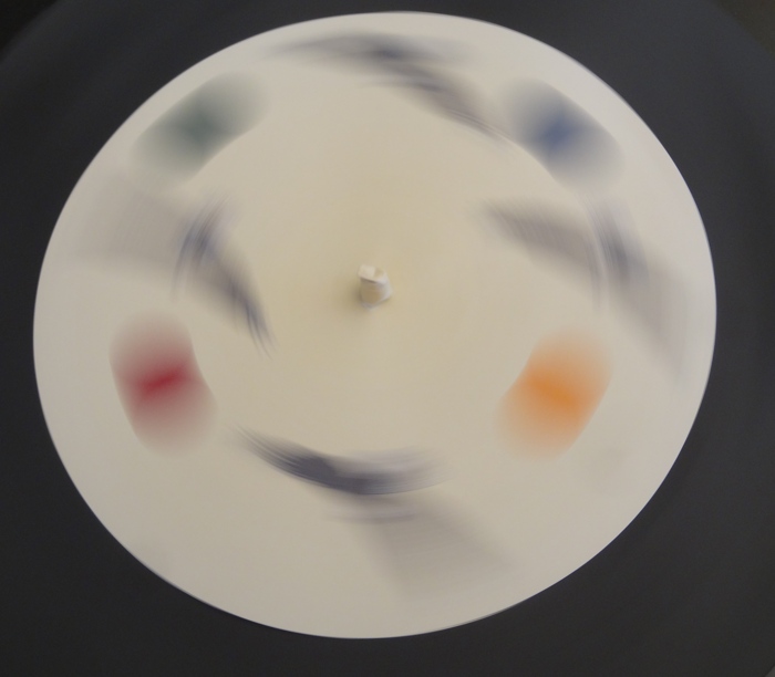
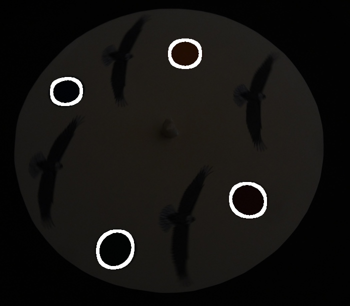
The map of LIP-additive Asplund distances is also useful for detecting moving objects. In Fig. 11, a white disk with patterns is mounted on a turn table of a record player. The patterns include four small coloured disks and confounding shapes (i.e. eagles). First of all, an image with good contrasts is captured with an appropriate exposure-time, 1/13 s (Fig. 11a). In this image, a circular probe is selected inside a coloured disk. The record player is then started up at a speed of 45 tours/min and two images are captured. The first image , which is acquired with the same exposure-time as the one of , is correctly exposed but blurred (Fig. 11b). As it is blurred, it is useless to detect the coloured disks. A second image is acquired at a shorter exposure-time of 1/160 s. This second image is not blurred but darker than (Fig. 11c). The map of LIP-additive Asplund distances of its complement, (Fig. 11e), is useful for the detection of the coloured disks. Those are detected by finding the regional minima of the map with sufficient height using the h-minima transform (Soille, 2004). The regional minima with too large or too small area are also removed. By comparing the map of the moving disk image (Fig. 11e) to the map of the fixed disk image (Fig. 11d), one can notice that they both present similar shapes and amplitudes although the images and are captured with different conditions. In particular, the kinetics of the scene are different because the disk is fixed or turning, and the lighting conditions differ significantly because the exposure-times are varying by a factor 12.
Fig. 10 shows the robustness of the LIP-additive Asplund metrics under intensity variations caused by variable exposure-times. Fig. 11 shows its efficiency to detect moving objects in dark images acquired with a small exposure-time which is necessary to capture an unblurred view of the object. Such cases occurs in many applications like medical images (Noyel et al., 2017) or industry (Noyel, 2011; Noyel et al., 2013). E.g. in industrial control the objects are often presented to the camera on a conveyor (linear, circular, etc.) whose speed varies with the production rate.
6.3.2 LIP-multiplicative metric: images acquired with a variable absorption of the medium
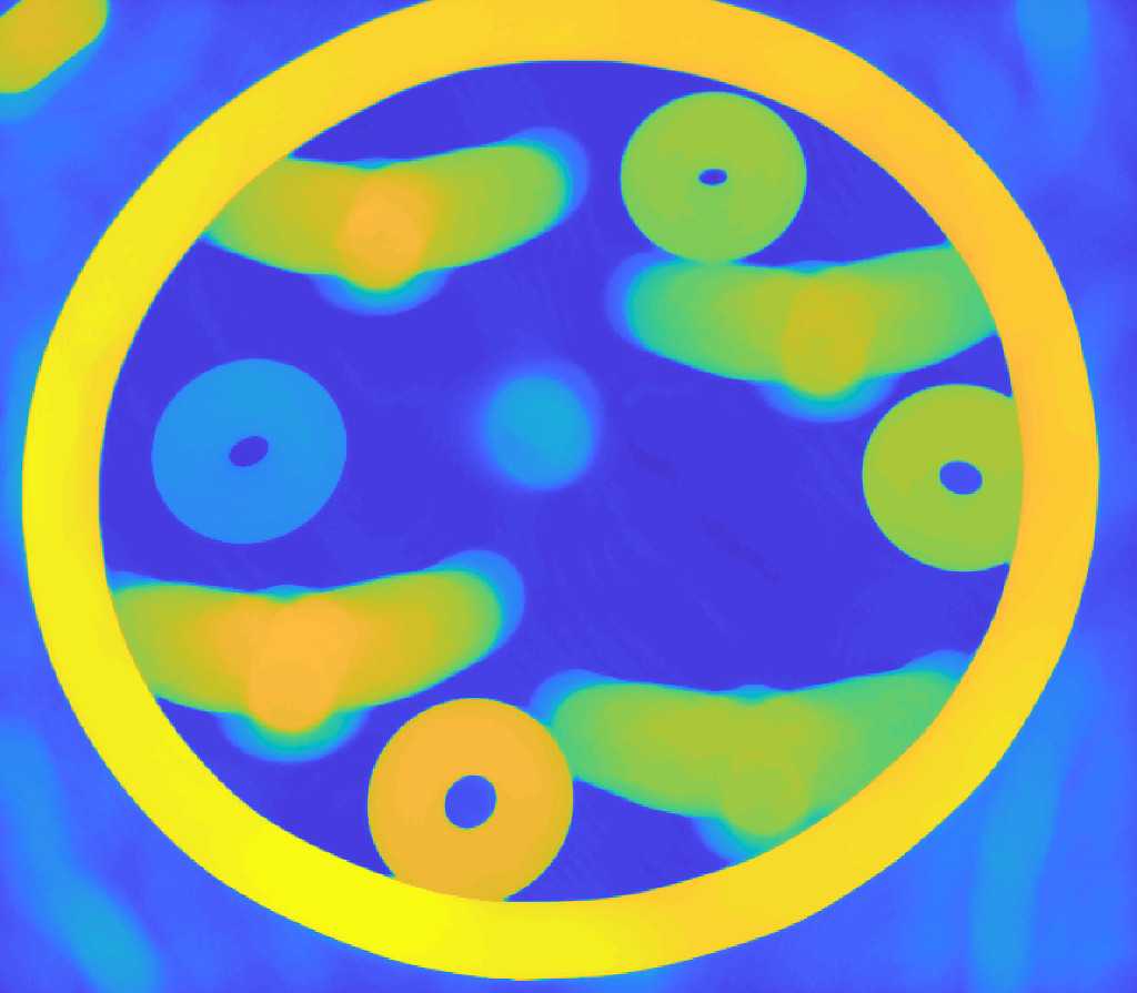
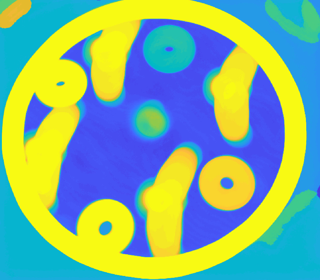
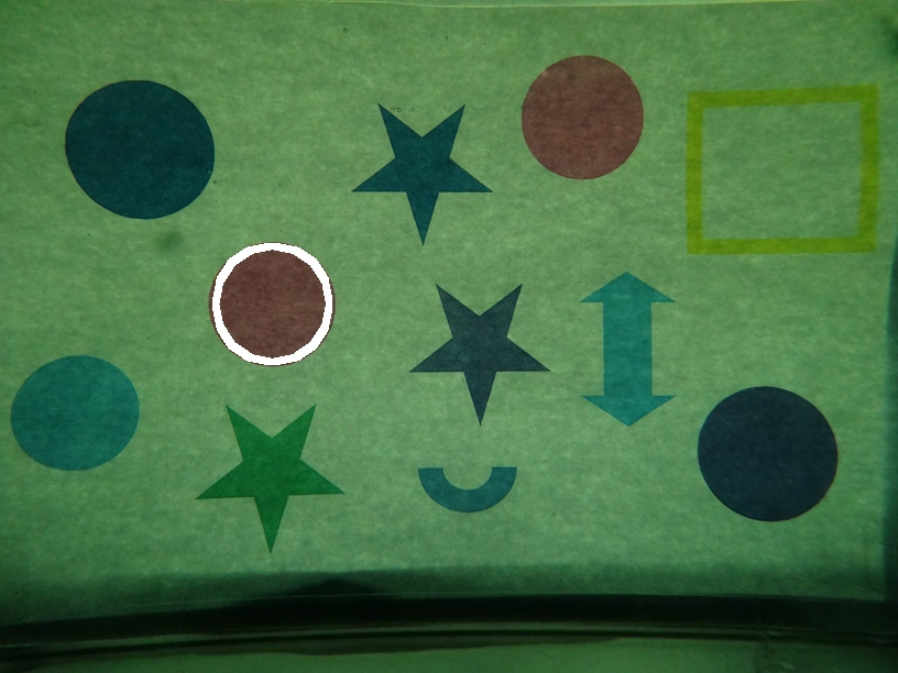
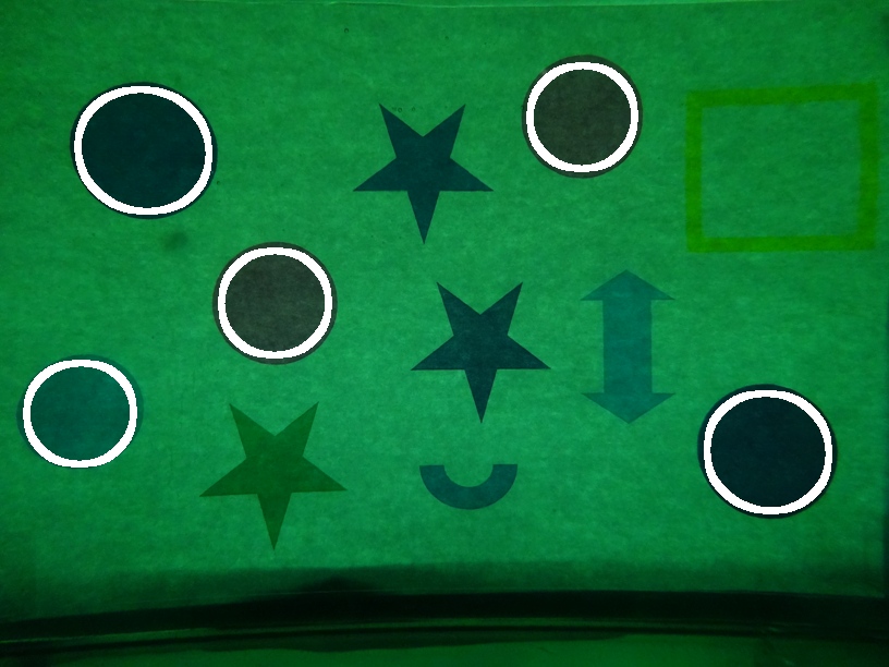
The independence of the map of LIP-multiplicative Asplund distances under light variations due to different absorption (or opacity) of the object is verified with a montage we made. It is composed of a transparent tank. A paper with motives is stuck on one of its sides. On the opposite side, a camera is disposed to capture an image of the paper through a medium composed of the tank and its contents: a green colourant diluted into water. Three images (Fig. 12a), (Fig. 12b) and (Fig. 12c) are acquired for increasing concentrations of the colourant: , and , where is the initial concentration of the colourant in the tank. One can notice that the image brightness decreases with the increase of the colourant concentration. A circular probe is manually selected in the brightest image in order to detect similar shapes in the two other images and . A map of Asplund distances is computed on the complement of each image with the same probe and the same tolerance parameter . One can notice that the three maps of images (Fig. 12d), (Fig. 12e) and (Fig. 12f) present similar amplitudes. They are segmented by the same thresholding technique – at the percentile – and two area openings in order to remove the too small and too large regions. The selected regions are then dilated for display purpose. One can notice that all the disks are detected in the two darkest images (Fig. 12b) and (Fig. 12c) using the probe extracted in the bright image . These results show the low sensitivity of the maps of LIP-multiplicative Asplund distances to light variations caused by different absorptions. Such a situation occurs in images acquired by transmission (e.g. X-rays, tomography, spectrophotometry, etc.) (Jourlin, 2016).
Remark 14.
In this section, probes with a circular invariance have been used to facilitate the presentation. However, the Asplund metrics are also efficient to detect non-circular objects with adapted probes. In addition, these metrics could be compared to the SIFT detector which is robust to lighting variations. The comparison has not been done in the sequel, because the robustness to lighting variations of the SIFT detector is not based on a physical law contrary to the Asplund metrics. However, Noyel et al. (2017) have shown that enhancing the contrast of images improves registration methods based on SIFT points (Lowe, 2004). We could therefore develop a SIFT in the LIP framework. These findings will be the studied in a future paper.
7 Conclusion
We have successfully presented a new framework of pattern matching robust to lighting variations between low-contrast and high-contrast images. It is composed of two metrics. Firstly, the LIP-multiplicative Asplund metric is robust to illumination changes due to variations of the object absorption or opacity. Secondly, the LIP-additive Asplund metric is robust to illumination changes caused by variations of the source intensity or of the camera exposure-time. Both metrics are respectively based on the multiplicative and the additive laws of the LIP model which give them strong optical properties. Both functional metrics are thereby theoretically insensitive to specific lighting variations. They extend to images the property of insensitivity to object magnification of the Asplund metric between binary shapes (Asplund, 1960; Grünbaum, 1963). After a presentation of the functional metrics and their properties, we have introduced robust to noise versions. We have demonstrated that the maps of Asplund distances between an image and a probe function are composed of Mathematical Morphology operations. Both maps of distances are especially related to the morphological operations of dilations and erosions for functions. Such a relation facilitates the programming of the maps of distances because these operations exist in numerous image processing libraries. The properties of both metrics have been then verified with simulated and real cases. Results have shown that the maps of LIP-multiplicative and LIP-additive Asplund distances are able to detect patterns in images acquired with different illuminations, caused by a stronger absorption of the object or by a shorter camera exposure-time, respectively. Importantly, the probe can be extracted in a highly contrasted image and the detection performed in a lowly contrasted image. Such properties pave the way to numerous applications where illumination variations are not controlled: e.g. in industry (Noyel et al., 2013), medicine (Noyel et al., 2014, 2017), traffic control (Geiger et al., 2014), safety and surveillance (Foresti et al., 2005), imaging of moving objects (Noyel, 2011), etc. In the future, these metrics will be extended to the analysis of colour and multivariate images starting from the preliminary ideas developed by Noyel and Jourlin (2015, 2017c). They will also be related to Logarithmic Mathematical Morphology (Noyel, 2019b).
Appendix A Appendix
The appendix is organised as follows. We will present the proofs of the propositions related to the LIP-multiplicative Asplund metric (Prop. 1 and 5) and to the LIP-additive metric (Prop. 6, 7, 8 and 9).
A.1 Proofs of propositions 1 and 5 related to the LIP-multiplicative Asplund metric
A.2 Proofs of propositions 6, 7, 8 and 9 related to the LIP-additive Asplund metric
Eq. 209 becomes therefore: . The last equality is due to the complete lattice structure. In a similar way, Eq. 218 becomes: . ∎
Appendix B Supplementary materials
Appendix C Acknowledgments
The authors are grateful to Dr Helen Boyle for her careful re-reading of the manuscript.
References
- Ancuti et al. (2018) Ancuti CO, Ancuti C, De Vleeschouwer C, Bekaert P (2018). Color balance and fusion for underwater image enhancement. IEEE T Image Process 27:379–93.
- Asplund (1960) Asplund E (1960). Comparison Between Plane Symmetric Convex Bodies and Parallelograms. Math Scand 8:171–80.
- Banon and Faria (1997) Banon G, Faria S (1997). Morphological approach for template matching. In: Proc X Brazilian Symp on Comput Graphics and Image Process.
- Banon and Barrera (1993) Banon GJF, Barrera J (1993). Decomposition of mappings between complete lattices by mathematical morphology, part I: General lattices. Signal Process 30:299 – 327.
- Barat et al. (2003) Barat C, Ducottet C, Jourlin M (2003). Pattern matching using morphological probing. In: IEEE Image Proc, vol. 1.
- Barat et al. (2010) Barat C, Ducottet C, Jourlin M (2010). Virtual double-sided image probing: A unifying framework for non-linear grayscale pattern matching. Pattern Recogn 43:3433–47.
- Bouaynaya and Schonfeld (2008) Bouaynaya N, Schonfeld D (2008). Theoretical foundations of spatially-variant mathematical morphology part II: Gray-level images. IEEE T Pattern Anal 30:837–50.
- Bourbaki (2007) Bourbaki N (2007). Intégration: Chapitres 1 à 4. Bourbaki, Nicolas. Springer Berlin Heidelberg.
- Brailean et al. (1991) Brailean J, Sullivan B, Chen C, Giger M (1991). Evaluating the EM algorithm for image processing using a human visual fidelity criterion. In: Int Conf Acoust Spee.
- Butterfly (2010) Butterfly (2010). Image from the YFCC100M dataset. http://www.flickr.com/photos/45563311@N04/4350683057/. Licence CC BY-NC-SA 2.0.
- Cantoni et al. (1998) Cantoni V, Cinque L, Guerra C, Levialdi S, Lombardi L (1998). 2-D object recognition by multiscale tree matching. Pattern Recogn 31:1443 – 1454.
- Carre and Jourlin (2014) Carre M, Jourlin M (2014). LIP operators: Simulating exposure variations to perform algorithms independent of lighting conditions. In: Int Conf on Multimedia Computing and Syst (ICMCS).
- Chen et al. (2006) Chen W, Er MJ, Wu S (2006). Illumination compensation and normalization for robust face recognition using discrete cosine transform in logarithm domain. IEEE T Syst Man Cy B 36:458–66.
- Deng (2011) Deng G (2011). A generalized unsharp masking algorithm. IEEE T Image Process 20:1249–61.
- Deshayes et al. (2015) Deshayes V, Guilbert P, Jourlin M (2015). How simulating exposure time variations in the LIP model. Application: moving objects acquisition. In: Acta Stereol., Proc. 14th ICSIA.
- Deza and Deza (2016) Deza MM, Deza E (2016). Encyclopedia of Distances. Springer Berlin Heidelberg.
- Dougherty (1991) Dougherty ER (1991). Application of the Hausdorff metric in gray-scale mathematical morphology via truncated umbrae. J Vis Commun Image R 2:177–87.
- Faraji and Qi (2016) Faraji MR, Qi X (2016). Face recognition under varying illuminations using logarithmic fractal dimension-based complete eight local directional patterns. Neurocomputing 199:16–30.
- Foresti et al. (2005) Foresti GL, Micheloni C, Snidaro L, Remagnino P, Ellis T (2005). Active video-based surveillance system: the low-level image and video processing techniques needed for implementation. IEEE Signal Proc Mag 22:25–37.
- Geiger et al. (2014) Geiger A, Lauer M, Wojek C, Stiller C, Urtasun R (2014). 3D traffic scene understanding from movable platforms. IEEE T Pattern Anal 36:1012–25.
- Grünbaum (1963) Grünbaum B (1963). Measures of symmetry for convex sets. In: P Symp Pure Math, vol. 7. Providence, R.I.: Amer. Math. Soc.
- Hautière et al. (2006) Hautière N, Labayrade R, Aubert D (2006). Real-time disparity contrast combination for onboard estimation of the visibility distance. IEEE T Intell Transp 7:201–12.
- Heijmans (1994) Heijmans H (1994). Morphological image operators. No. vol. 25 in Adv Imag Elect Phys: Supplement. Academic Press.
- Heijmans and Ronse (1990) Heijmans H, Ronse C (1990). The algebraic basis of mathematical morphology I. Dilations and erosions. Comput Vision Graphics and Image Process 50:245 – 295.
- Hussain Shah et al. (2015) Hussain Shah J, Sharif M, Raza M, Murtaza M, Ur-Rehman S (2015). Robust face recognition technique under varying illumination. J Appl Res Technol 13:97–105.
- Huttenlocher et al. (1993) Huttenlocher DP, Klanderman GA, Rucklidge WJ (1993). Comparing images using the Hausdorff distance. IEEE T Pattern Anal 15:850–63.
- Jourlin (2016) Jourlin M (2016). Logarithmic Image Processing: Theory and Applications, vol. 195 of Adv Imag Elect Phys. Elsevier Science.
- Jourlin et al. (2012) Jourlin M, Carré M, Breugnot J, Bouabdellah M (2012). Chapter 7 - Logarithmic image processing: Additive contrast, multiplicative contrast, and associated metrics. In: Adv Imag Elect Phys, vol. 171. Elsevier, 357 – 406.
- Jourlin et al. (2014) Jourlin M, Couka E, Abdallah B, Corvo J, Breugnot J (2014). Asplund’s metric defined in the Logarithmic Image Processing (LIP) framework: A new way to perform double-sided image probing for non-linear grayscale pattern matching. Pattern Recogn 47:2908 – 2924.
- Jourlin and Pinoli (1988) Jourlin M, Pinoli J (1988). A model for logarithmic image-processing. J Microsc Oxford 149:21–35.
- Jourlin and Pinoli (2001) Jourlin M, Pinoli J (2001). Logarithmic image processing: The mathematical and physical framework for the representation and processing of transmitted images. In: Adv Imag Elect Phys, vol. 115. Elsevier, 129 – 196.
- Jourlin and Pinoli (1995) Jourlin M, Pinoli JC (1995). Image dynamic range enhancement and stabilization in the context of the logarithmic image processing model. Signal Process 41:225 – 237.
- Khosravi and Schafer (1996) Khosravi M, Schafer R (1996). Template matching based on a grayscale hit-or-miss transform. IEEE T Image Process 5:1060–6.
- Lai et al. (2014) Lai ZR, Dai DQ, Ren CX, Huang KK (2014). Multilayer surface albedo for face recognition with reference images in bad lighting conditions. IEEE T Image Process 23:4709–23.
- Li and Lu (2009) Li J, Lu BL (2009). An adaptive image Euclidean distance. Pattern Recogn 42:349 – 357.
- Lowe (2004) Lowe DG (2004). Distinctive image features from scale-invariant keypoints. Int J Comput Vision 60:91–110.
- Matheron (1967) Matheron G (1967). Eléments pour une théorie des milieux poreux. Masson, Paris.
- Mayet et al. (1996) Mayet F, Pinoli JC, Jourlin M (1996). Physical justifications and applications of the LIP model for the processing of transmitted light images. Trait Signal 13:251 – 262.
- Messelodi et al. (2005) Messelodi S, Modena CM, Segata N, Zanin M (2005). A Kalman filter based background updating algorithm robust to sharp illumination changes. In: Lect Notes Comput Sc, vol. 3617. Berlin, Heidelberg: Springer.
- Meylan and Susstrunk (2006) Meylan L, Susstrunk S (2006). High dynamic range image rendering with a retinex-based adaptive filter. IEEE T Image Process 15:2820–30.
- Najman and Talbot (2013) Najman L, Talbot H (2013). Mathematical Morphology: From Theory to Applications. Wiley-Blackwell, 1st ed.
- Navarro et al. (2014) Navarro L, Courbebaisse G, Jourlin M (2014). Chapter two - Logarithmic wavelets. In: Adv Imag Elect Phys, vol. 183. Elsevier, 41 – 98.
- Navarro et al. (2013) Navarro L, Deng G, Courbebaisse G (2013). The symmetric logarithmic image processing model. Digital Signal Process 23:1337 – 1343.
- Noyel (2011) Noyel G (2011). Method of monitoring the appearance of the surface of a tire. https://patentscope.wipo.int/search/en/WO2011131410. Patent, International PCT no WO2011131410 (A1). Also published as: US9002093 (B2), FR2959046 (B1), JP5779232 (B2), EP2561479 (A1), CN102844791 (B), BR112012025402 (A2).
- Noyel (2019a) Noyel G (2019a). A link between the multiplicative and additive functional Asplund’s metrics. In: Lect Notes Comp Sc, vol. 11564. Cham: Springer Int Publishing.
- Noyel (2019b) Noyel G (2019b). Logarithmic Mathematical Morphology: A new framework adaptive to illumination changes. In: Lect Notes Comp Sc, vol. 11401. Cham: Springer Int Publishing.
- Noyel et al. (2014) Noyel G, Angulo J, Jeulin D, Balvay D, Cuenod CA (2014). Multivariate mathematical morphology for DCE-MRI image analysis in angiogenesis studies. Image Anal Stereol 34:1–25.
- Noyel et al. (2013) Noyel G, Jeulin D, Parra-Denis E, Bilodeau M (2013). Method of checking the appearance of the surface of a tyre. https://patentscope.wipo.int/search/en/WO2013045593. Patent, International PCT no WO2013045593 (A1). Also published as US9189841 (B2), FR2980735 (B1), EP2761587 (A1), CN103843034 (A).
- Noyel and Jourlin (2015) Noyel G, Jourlin M (2015). Asplund’s metric defined in the logarithmic image processing (LIP) framework for colour and multivariate images. In: IEEE Image Proc.
- Noyel and Jourlin (2017a) Noyel G, Jourlin M (2017a). Double-sided probing by map of Asplund’s distances using Logarithmic Image Processing in the framework of Mathematical Morphology. In: Lect Notes Comput Sc, vol. 10225. Cham: Springer Int Publishing.
- Noyel and Jourlin (2017b) Noyel G, Jourlin M (2017b). A simple expression for the map of Asplund’s distances with the multiplicative Logarithmic Image Processing (LIP) law. Personal communication, Eur Congr Stereology and Image Anal, Kaiserslautern, Germany.
- Noyel and Jourlin (2017c) Noyel G, Jourlin M (2017c). Spatio-colour Asplund’s metric and Logarithmic Image Processing for Colour images (LIPC). In: Lect Notes Comp Sc, vol. 10125. Cham: Springer.
- Noyel et al. (2017) Noyel G, Thomas R, Bhakta G, Crowder A, Owens D, Boyle P (2017). Superimposition of eye fundus images for longitudinal analysis from large public health databases. Biomed Phys Eng Express 3:045015.
- Odone et al. (2001) Odone F, Trucco E, Verri A (2001). General purpose matching of grey level arbitrary images. In: Lect Notes Comput Sc, vol. 2059. Berlin, Heidelberg: Springer.
- Peng and Cosman (2017) Peng YT, Cosman PC (2017). Underwater image restoration based on image blurriness and light absorption. IEEE T Image Process 26:1579–94.
- Pizer et al. (1987) Pizer SM, Amburn EP, Austin JD, Cromartie R, Geselowitz A, Greer T, ter Haar Romeny B, Zimmerman JB, Zuiderveld K (1987). Adaptive histogram equalization and its variations. Comput Vis Graph Image Process 39:355 – 368.
- Salti et al. (2015) Salti S, Petrelli A, Tombari F, Fioraio N, Stefano LD (2015). Traffic sign detection via interest region extraction. Pattern Recogn 48:1039 – 1049.
- Savvides and Kumar (2003) Savvides M, Kumar BV (2003). Illumination normalization using logarithm transforms for face authentication. In: Lect Notes Comp Sc, vol. 2688. Springer Berlin Heidelberg.
- Serra (1982) Serra J (1982). Image Analysis and Mathematical Morphology, vol. 1. New York: Academic Press.
- Serra (1988) Serra J, ed. (1988). Image analysis and Mathematical Morphology: Theoretical advances, vol. 2. Academic Press.
- Shan et al. (2003) Shan S, Gao W, Cao B, Zhao D (2003). Illumination normalization for robust face recognition against varying lighting conditions. In: IEEE Int SOI Conf.
- Soille (2004) Soille P (2004). Morphological Image Analysis: Principles and Applications. Berlin, Heidelberg: Springer, 2nd ed.
- Thomee et al. (2016) Thomee B, Shamma DA, Friedland G, Elizalde B, Ni K, Poland D, Borth D, Li LJ (2016). YFCC100M: The new data in multimedia research. Commun ACM 59:64–73.
- van de Gronde and Roerdink (2014) van de Gronde JJ, Roerdink JBTM (2014). Group-invariant colour morphology based on frames. IEEE T Image Process 23:1276–88.
- Wang et al. (2005) Wang L, Zhang Y, Feng J (2005). On the Euclidean distance of images. IEEE T Pattern Anal 27:1334–9.
- Xie and Lam (2005) Xie X, Lam KM (2005). Face recognition under varying illumination based on a 2D face shape model. Pattern Recogn 38:221 – 230.