High-order gas-kinetic scheme with three-dimensional WENO reconstruction for the Euler and Navier-Stokes solutions

Abstract

In this paper, a simple and efficient third-order weighted essentially non-oscillatory (WENO) reconstruction is developed for three-dimensional flows, in which the idea of two-dimensional WENO-AO scheme on unstructured meshes [43] is adopted. In the classical finite volume type WENO schemes, the linear weights for the candidate stencils are obtained by solving linear systems at Gaussian quadrature points of cell interface. For the three-dimensional scheme, such operations at twenty-four Gaussian quadrature points of a hexahedron would reduce the efficiency greatly, especially for the moving-mesh computation. Another drawback of classical WENO schemes is the appearance of negative weights with irregular local topology, which affect the robustness of spatial reconstruction. In such three-dimensional WENO-AO scheme, a simple strategy of selecting big stencil and sub-stencils for reconstruction is proposed. With the reconstructed quadratic polynomial from big stencil and linear polynomials from sub-stencils, the linear weights are chosen as positive numbers with the requirement that their sum equals one and be independent of local mesh topology. With such WENO reconstruction, a high-order gas-kinetic scheme (HGKS) is developed for both three-dimensional inviscid and viscous flows. Taken the grid velocity into account, the scheme is extended into the moving-mesh computation as well. Numerical results are provided to illustrate the good performance of such new finite volume WENO schemes. In the future, such WENO reconstruction will be extended to the unstructured meshes.

1 Introduction

In recent decades, there have been continuous interests and efforts on the development of high-order schemes for compressible flows. There have been a gigantic number of publications about the introduction and survey of high-order schemes, including discontinuous Galerkin (DG) [9, 10], essentially nonoscillatory (ENO), weighted ENO (WENO) schemes, etc. In this paper, we mainly focus on the finite volume type schemes. The ENO schemes were proposed in [15, 33] and successfully applied to solve the hyperbolic conservation laws and other convection dominated problems. The “smoothest” stencil is selected among several candidates to achieve high-order accuracy in the smooth region and keep essentially non-oscillatory near discontinuities. For unstructured meshes, the ENO scheme was developed as well [1]. Following the ENO scheme, the WENO schemes [25, 20, 16, 5] were developed. With the nonlinear convex combination of candidate polynomials, WENO scheme achieves higher order of accuracy and keeps non-oscillatory property essentially. Compared with ENO scheme, the WENO schemes improve robustness, smoothness of fluxes, steady-state convergence and efficiency in the computation. On the unstructured meshes, the WENO schemes were also developed [17]. Similar with the one-dimensional WENO scheme, the high-order of accuracy is obtained by the combination of lower order polynomials. However, its successful application is limited by the appearance of negative linear weights and very large linear weights, which appears commonly on the unstructured meshes. For a mesh that is close to the regular meshes, such WENO scheme works well by a regrouping approach to avoid negative weights. However, for a mesh with lower quality, the large linear weights appears and WENO schemes become unstable even for the smooth flows. In order to avoid the negative linear weights and very large linear weights, many WENO schemes were proposed [32, 40, 11]. Instead of concentrating on the reconstruction of interface values, there exist another class of WENO methods to reconstruct a polynomial inside each cell based on all stencils, which is also named as the WENO with adaptive order (WENO-AO) method [2, 42, 43]. The linear weights are artificially set to be positive numbers with the requirement that their sum equals to one. With the non-linear weights, the WENO-AO schemes could achieve the optimal order of accuracy in smooth region, and automatically approach to the smoothest quadratic sub-stencil in discontinuous region using the same stencils from original WENO scheme. The independence of linear weights on local topology not only improve the efficiency, but also reduces the complexity of the classical WENO scheme.

In the past decades, the gas-kinetic schemes (GKS) based on the Bhatnagar-Gross-Krook (BGK) model [4, 8] have been developed systematically for the computations from low speed flow to supersonic one [38, 39]. Different from the numerical methods based on Riemann fluxes [35], a time-dependent gas distribution function is provided at the cell interface for inviscid and viscous terms together. With such spatial and temporal coupled gas distribution function, the one-stage third-order GKS was developed [24], which integrates the flux function over a time step analytically without employing the multi-stage Runge-Kutta time stepping techniques [14]. However, with the one-stage gas evolution model, the formulation of GKS becomes very complicated for the further improvement [26]. Recently, based on the time-dependent flux function, a two-stage fourth-order method was developed for Lax-Wendroff type flow solvers [3, 39], particularly for the hyperbolic conservation laws [23, 13, 28, 19]. With the two-stage temporal discretization, a reliable framework was provided for developing fourth-order and even higher-order accuracy [41]. For the construction of high-order scheme, a spatial-temporal coupled evolution model becomes important, and the delicate flow structures depend on the quality of flow solvers [18, 19]. With the dimensional-by-dimensional WENO reconstruction, the high-order gas-kinetic scheme has been extended to three-dimensional computation with the structured meshes [29], especially for the direct numerical simulation for the compressible isotropic turbulence [7].

To simulate the flow with complicated geometry, a high-order gas-kinetic scheme was proposed with the unstructured WENO reconstruction, and extended to the moving-mesh computation [30]. The accuracy and geometric conservation law are well preserved even with the largely deforming mesh. However, choosing sub-stencils from big stencil and solving linear weights at Gaussian quadrature points would make the reconstruction extremely complicated for three-dimensional flows. In this paper, a simple and efficient third-order WENO-AO scheme is developed for three-dimensional flows to overcome the drawbacks above, in which the three-dimensional structured mesh is considered for simplicity. With the such reconstruction, a high-order gas-kinetic scheme (HGKS) is developed for both Euler and Navier-Stokes solutions. In such three-dimensional WENO-AO scheme, the strategy of selecting big stencil and candidates of sub-stencils for reconstruction is proposed. Based on the reconstructed quadratic polynomial for big stencil and linear polynomials for sub-stencils, the spatial independent linear weights are used, which have fixed values and become positive. With the smooth indicator, the nonlinear weights can be constructed. Meanwhile, the point-values and slopes for non-equilibrium part of gas distribution function can be reconstructed at all Gaussian quadrature points. Through particle colliding procedure, the point-values and slopes for equilibrium part are obtained simultaneously and an extra reconstruction for equilibrium state in the classical HGKS is avoided. Taken the grid velocity into account, such scheme can be also extended into the moving-mesh computation. For the mesh with non-coplanar vertexes, which is commonly generated in the moving-mesh computation, the trilinear interpolation is used to parameterize the hexahedron, and the bilinear interpolation is used to parameterize the interface of hexahedron. Extensive numerical results are provided to illustrate the good performance of such new finite volume WENO schemes. The optimal order of accuracy in smooth regions can be obtained, and the strong discontinuities are also well captured.

This paper is organized as follows. In Section 2, third-order WENO reconstruction is introduced. The high-order gas-kinetic scheme is presented in Section 3. In Section 4, we present the extension to ALE framework. Section 5 includes numerical examples to validate the current algorithm. The last section is the conclusion.

2 Third-order WENO reconstruction

In this section, an efficient and simple WENO scheme is proposed for three-dimensional flows, and the idea comes from the two-dimensional WENO-AO scheme on unstructured meshes [43]. For simplicity, the reconstruction is developed on structured meshes and the extension to unstructured meshes will be developed in the future. For a piecewise smooth function $Q(\bm{x})$ over cell $\Omega_{ijk}$, a polynomial $P_{0}(\bm{x})$ with degree $r$ can be constructed to approximate $Q(\bm{x})$ as follows

$$p(\bm{x})=Q(\bm{x})+\mathcal{O}(h^{r+1}),$$

where $|\Omega_{ijk}|$ is volume of $\Omega_{ijk}$ and $h\sim|\Omega_{ijk}|^{1/3}$ is the cell size. In order to achieve third-order accuracy and satisfy conservative property, the following quadratic polynomial is constructed

$$P_{0}(\bm{x})=Q_{ijk}+\sum_{|n|=1}^{2}a_{n}p_{n}(\bm{x}),$$ (1)

where $Q_{ijk}$ is the cell averaged variables of $Q(\bm{x})$ over $\Omega_{ijk}$, $n=(n_{1},n_{2},n_{3})$, $|n|=n_{1}+n_{2}+n_{3}$ and

$$\displaystyle p_{n}(\bm{x})=x^{n_{1}}y^{n_{2}}z^{n_{3}}-\frac{1}{\left|\Omega_{ijk}\right|}\iiint_{\Omega_{ijk}}x^{n_{1}}y^{n_{2}}z^{n_{3}}\text{d}V.$$

In order to fully determine this polynomial, a big stencil $S$ for $\Omega_{ijk}$, which is shown in Fig.1, is selected as follows

$$S=\{\Omega_{i+i_{0},j+j_{0},k+k_{0}},~{}i_{0},j_{0},k_{0}=-1,0,1,~{}i_{0}\cdot j_{0}\cdot k_{0}\neq\pm 1\}.$$

The following constrains need to be satisfied in the big stencil

$$\frac{1}{\left|\Omega_{i^{\prime}j^{\prime}k^{\prime}}\right|}\iiint_{\Omega_{i^{\prime}j^{\prime}k^{\prime}}}P_{0}(\bm{x})\text{d}V=Q_{i^{\prime}j^{\prime}k^{\prime}},~{}\Omega_{i^{\prime}j^{\prime}k^{\prime}}\in S.$$

An over determined linear system will be generated, and the coefficients $a_{n}$ in Eq.(1) can be determined by the least square method.

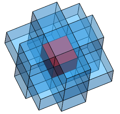
Figure 1: Stencils of cell $\Omega_{ijk}$ (red cubic) for three-dimensional reconstruction.

Twenty-four candidate sub-stencils are selected from the big stencil as well, and one third of them are given as follows

$$S_{1}=\{\Omega_{i,j,k},\Omega_{i+1,j,k},\Omega_{i,j+1,k},\Omega_{i+1,j+1,k},\Omega_{i,j,k+1}\},$$

$$S_{2}=\{\Omega_{i,j,k},\Omega_{i-1,j,k},\Omega_{i,j+1,k},\Omega_{i-1,j+1,k},\Omega_{i,j,k+1}\},$$

$$S_{3}=\{\Omega_{i,j,k},\Omega_{i+1,j,k},\Omega_{i,j-1,k},\Omega_{i+1,j-1,k},\Omega_{i,j,k+1}\},$$

$$S_{4}=\{\Omega_{i,j,k},\Omega_{i-1,j,k},\Omega_{i,j+1,k},\Omega_{i-1,j-1,k},\Omega_{i,j,k+1}\},$$

$$S_{5}=\{\Omega_{i,j,k},\Omega_{i+1,j,k},\Omega_{i,j+1,k},\Omega_{i+1,j+1,k},\Omega_{i,j,k-1}\},$$

$$S_{6}=\{\Omega_{i,j,k},\Omega_{i-1,j,k},\Omega_{i,j+1,k},\Omega_{i-1,j+1,k},\Omega_{i,j,k-1}\},$$

$$S_{7}=\{\Omega_{i,j,k},\Omega_{i+1,j,k},\Omega_{i,j-1,k},\Omega_{i+1,j-1,k},\Omega_{i,j,k-1}\},$$

$$S_{8}=\{\Omega_{i,j,k},\Omega_{i-1,j,k},\Omega_{i,j+1,k},\Omega_{i-1,j-1,k},\Omega_{i,j,k-1}\}.$$

Symmetrically, another two thirds of the sub-stencils can be fully given. For each sub-stencil, a linear polynomial $P_{m}(\bm{x}),m=1,...,24$ is constructed

$$P_{m}(\bm{x})=Q_{ijk}+\sum_{|n|=1}b_{n}^{m}p_{n}(\bm{x}).$$ (2)

The following constrains need to be satisfied for cells in the candidate sub-stencils

$$\frac{1}{\left|\Omega_{i^{\prime}j^{\prime}k^{\prime}}\right|}\iiint_{\Omega_{i^{\prime}j^{\prime}k^{\prime}}}P_{m}(\bm{x})\text{d}x\text{d}y=Q_{i^{\prime}j^{\prime}k^{\prime}},~{}\Omega_{i^{\prime}j^{\prime}k^{\prime}}\in S_{m}.$$

The coefficients $b_{n}^{m}$ in Eq.(2) can be determined by the least square method as well.

With the reconstructed polynomials, the quadratic polynomial $P_{0}(\bm{x})$ can be rearranged as follows

$$P_{0}(\bm{x})=\gamma_{0}(\frac{1}{\gamma_{0}}P_{0}(\bm{x})-\sum_{m=1}^{24}\frac{\gamma_{m}}{\gamma_{0}}P_{m}(\bm{x}))+\sum_{m=1}^{24}\gamma_{m}P_{m}(\bm{x}),$$

where $\gamma_{m}>0,m=0,...,24$ are the linear weights, $\gamma_{0}=1-24\Gamma,\gamma_{i}=\Gamma,i=1,...,24$. In the computation, $\Gamma=0.0025$ is suggested. To deal with the discontinuities, the non-linear weights are introduced. The reconstructed point-value to approximate $Q(\bm{x}_{G})$ at Gaussian quadrature point is given as

$$\widetilde{P}_{0}(\bm{x}_{G})=\overline{\omega}_{0}(\frac{1}{\gamma_{0}}P_{0}(\bm{x}_{G})-\sum_{m=1}^{24}\frac{\gamma_{m}}{\gamma_{0}}P_{m}(\bm{x}_{G}))+\sum_{m=1}^{24}\overline{\omega}_{m}P_{m}(\bm{x}_{G}).$$

The non-linear weights $\omega_{m}$ and normalized non-linear weights $\overline{\omega}_{m}$ are defined as

$$\overline{\omega}_{m}=\frac{\omega_{m}}{\sum_{m=0}^{24}\omega_{m}},m=0,...,24$$

and

$$\omega_{m}=\gamma_{m}\Big{[}1+\Big{(}\frac{\tau}{\beta_{m}+\epsilon}\Big{)}\Big{]},$$ (3)

where $\epsilon$ is a small positive number. The smooth indicator $\beta_{m}$ is given as

$$\beta_{m}=\sum_{|l|=1}^{r_{m}}|\Omega_{ijk}|^{\frac{2|l|}{3}-1}\int_{\Omega_{ijk}}\Big{(}\frac{\partial^{l}P_{m}}{\partial_{x}^{l_{1}}\partial_{y}^{l_{2}}\partial_{z}^{l_{3}}}(x,y,z)\Big{)}^{2}\text{d}V,$$ (4)

where $r_{0}=2$ and $r_{m}=1,m\neq 0$. In order to achieve the optimal order of accuracy, the parameter $\tau$ is chosen as

$$\tau=\sum_{m=1}^{24}\Big{(}\frac{|\beta_{0}-\beta_{m}|}{24}\Big{)}.$$ (5)

According to the Taylor expansion, the smooth indicator Eq.(4) can be rewritten as

$$\beta_{0}= \Big{(}\big{(}\frac{\partial Q}{\partial x}\big{)}^{2}+\big{(}\frac{\partial Q}{\partial y}\big{)}^{2}+\big{(}\frac{\partial Q}{\partial z}\big{)}^{2}\Big{)}\Big{|}_{\bm{x}_{0}}|\Omega_{ijk}|^{2/3}(1+\mathcal{O}(|\Omega_{ijk}|^{2/3})),$$

$$\beta_{m}= \Big{(}\big{(}\frac{\partial Q}{\partial x}\big{)}^{2}+\big{(}\frac{\partial Q}{\partial y}\big{)}^{2}+\big{(}\frac{\partial Q}{\partial z}\big{)}^{2}\Big{)}\Big{|}_{\bm{x}_{0}}|\Omega_{ijk}|^{2/3}(1+\mathcal{O}(|\Omega_{ijk}|^{1/3})),$$

where $m=1,...,24$. According to the definition of the parameter $\tau$ in Eq.(5), the non-linear weights can be approximated as

$$\overline{\omega}_{m}\sim\omega_{m}=\gamma_{m}(1+\mathcal{O}(h)),$$

which ensures the optimal order of accuracy of the current scheme.

To examine the accuracy of new WENO reconstruction, it is supposed that the following sufficient condition is satisfied for the nonlinear weight

$$\omega_{m}=\gamma_{m}(1+\mathcal{O}(h^{k})).$$ (6)

For the quadratic polynomial $P_{0}(\bm{x})$, the error can be written as

$$P_{0}(\bm{x}_{G})=Q(\bm{x}_{G})+A(\bm{x}_{G})h^{3}+\mathcal{O}(h^{4}),$$

where $Q(\bm{x}_{G})$ is the exact solution at the Gaussian quadrature point $\bm{x}_{G}$. For the linear polynomial $P_{m}(\bm{x}_{G})$, the error can be written as

$$P_{m}(\bm{x}_{G})=Q(\bm{x}_{G})+B_{m}(\bm{x}_{G})h^{2}+\mathcal{O}(h^{3}),$$

The reconstructed point value with non-linear weights can be written as

$$\widetilde{P}_{0}(\bm{x}_{G})= \frac{\overline{\omega}_{0}}{\gamma_{0}}P_{0}(\bm{x}_{G})+\sum_{m=1}^{24}(\overline{\omega}_{m}-\frac{\overline{\omega}_{0}\gamma_{m}}{\gamma_{0}})P_{m}(\bm{x}_{G}),$$

$$= \frac{\overline{\omega}_{0}}{\gamma_{0}}(Q(\bm{x}_{G})+A(\bm{x}_{G})h^{3}+\mathcal{O}(h^{4}))+\sum_{m=1}^{24}(\overline{\omega}_{m}-\frac{\overline{\omega}_{0}\gamma_{m}}{\gamma_{0}})(Q(\bm{x}_{G})+B_{m}(\bm{x}_{G})h^{2}+\mathcal{O}(h^{3}))$$

$$= Q(\bm{x}_{G})+\frac{\overline{\omega}_{0}}{\gamma_{0}}(A(\bm{x}_{G})h^{3}+\mathcal{O}(h^{4}))+\sum_{m=1}^{24}(\overline{\omega}_{m}-\overline{\omega}_{0}\frac{\gamma_{m}}{\gamma_{0}})(B_{m}(\bm{x}_{G})h^{2}+\mathcal{O}(h^{3}))$$

$$= Q(\bm{x}_{G})+A(\bm{x}_{G})h^{3}+\sum_{m=1}^{24}B_{m}(\bm{x}_{G})h^{2+k}+\mathcal{O}(h^{3+k}+h^{4}).$$

Thus, to achieve the third-order accuracy, $k=1$ is needed in Eq.(6).

With the reconstructed polynomial, the spatial derivatives at Gaussian quadrature point, which will be used in the gas-kinetic solver, can be given as follows

$$\partial_{x}\widetilde{P}_{0}(\bm{x}_{G})=\overline{\omega}_{0}(\frac{1}{\gamma_{0}}\partial_{x}P_{0}(\bm{x}_{G})-\sum_{m=1}^{24}\frac{\gamma_{m}}{\gamma_{0}}\partial_{x}P_{m}(\bm{x}_{G}))+\sum_{m=1}^{24}\overline{\omega}_{m}\partial_{x}P_{m}(\bm{x}_{G}),$$

$$\partial_{y}\widetilde{P}_{0}(\bm{x}_{G})=\overline{\omega}_{0}(\frac{1}{\gamma_{0}}\partial_{y}P_{0}(\bm{x}_{G})-\sum_{m=1}^{24}\frac{\gamma_{m}}{\gamma_{0}}\partial_{y}P_{m}(\bm{x}_{G}))+\sum_{m=1}^{24}\overline{\omega}_{m}\partial_{y}P_{m}(\bm{x}_{G}),$$

$$\partial_{z}\widetilde{P}_{0}(\bm{x}_{G})=\overline{\omega}_{0}(\frac{1}{\gamma_{0}}\partial_{z}P_{0}(\bm{x}_{G})-\sum_{m=1}^{24}\frac{\gamma_{m}}{\gamma_{0}}\partial_{z}P_{m}(\bm{x}_{G}))+\sum_{m=1}^{24}\overline{\omega}_{m}\partial_{z}P_{m}(\bm{x}_{G}).$$

Remark 1

In this section, we present one choice of big stencil and candidates of sub-stencils, which work well for the numerical tests given in the following section. However, such choice is not unique and may not be optimal. For example, the following big stencil $S^{\prime}$

$$S^{\prime}=S\cup\{\Omega_{i\pm 2,j,k},\Omega_{i,j\pm 2,k},\Omega_{i,j,k\pm 2}\}.$$

and candidate sub-stencils $S^{\prime}_{i},i=1,..,8,$

$$S_{1}^{\prime}=\{\Omega_{i,j,k},\Omega_{i+1,j,k},\Omega_{i,j+1,k},\Omega_{i,j,k+1}\},~{}S_{5}^{\prime}=\{\Omega_{i,j,k},\Omega_{i+1,j,k},\Omega_{i,j+1,k},\Omega_{i,j,k-1}\},$$

$$S_{2}^{\prime}=\{\Omega_{i,j,k},\Omega_{i-1,j,k},\Omega_{i,j+1,k},\Omega_{i,j,k+1}\},~{}S_{6}^{\prime}=\{\Omega_{i,j,k},\Omega_{i-1,j,k},\Omega_{i,j+1,k},\Omega_{i,j,k-1}\},$$

$$S_{3}^{\prime}=\{\Omega_{i,j,k},\Omega_{i+1,j,k},\Omega_{i,j-1,k},\Omega_{i,j,k+1}\},~{}S_{7}^{\prime}=\{\Omega_{i,j,k},\Omega_{i+1,j,k},\Omega_{i,j-1,k},\Omega_{i,j,k-1}\},$$

$$S_{4}^{\prime}=\{\Omega_{i,j,k},\Omega_{i-1,j,k},\Omega_{i,j+1,k},\Omega_{i,j,k+1}\},~{}S_{8}^{\prime}=\{\Omega_{i,j,k},\Omega_{i-1,j,k},\Omega_{i,j+1,k},\Omega_{i,j,k-1}\}.$$

can be used as substitutions respectively. These substitutions work as well in the computation.

As mentioned in the introduction, the vertexes of hexahedron may become non-coplanar during the moving mesh procedure, which introduces difficulty to preserve the high-order accuracy and geometric conservation law. In this paper, the trilinear interpolation is used to describe the hexahedron with non-coplanar vertex as follows

$$\bm{X}(\xi,\eta,\zeta)=\sum_{i=1}^{8}\bm{x}_{i}\psi_{i}(\xi,\eta,\zeta),$$

where $(\xi,\eta,\zeta)\in[-1/2,1/2]^{3}$, $\bm{x}_{i}$ is the vertex of a hexahedron and $\psi_{i}$ is the base function

$$\psi_{1}=\frac{1}{8}(1-2\xi)(1-2\eta)(1-2\zeta),~{}\psi_{2}=\frac{1}{8}(1-2\xi)(1-2\eta)(1+2\zeta),$$

$$\psi_{3}=\frac{1}{8}(1-2\xi)(1+2\eta)(1-2\zeta),~{}\psi_{4}=\frac{1}{8}(1-2\xi)(1+2\eta)(1+2\zeta),$$

$$\psi_{5}=\frac{1}{8}(1+2\xi)(1-2\eta)(1-2\zeta),~{}\psi_{6}=\frac{1}{8}(1+2\xi)(1-2\eta)(1+2\zeta),$$

$$\psi_{7}=\frac{1}{8}(1+2\xi)(1+2\eta)(1-2\zeta),~{}\psi_{8}=\frac{1}{8}(1+2\xi)(1+2\eta)(1+2\zeta).$$

For the hexahedron with non-coplanar vertex, the triple integral over the parameterized control volume can be given by

$$\iiint_{\Omega}x^{a}y^{b}z^{c}\text{d}x\text{d}y\text{d}z =\iiint_{\Omega}x^{a}y^{b}z^{c}(\xi,\eta,\zeta)\Big{|}\frac{\partial(x,y,z)}{\partial(\xi,\eta,\zeta)}\Big{|}\text{d}\xi\text{d}\eta\text{d}\zeta.$$

For simplicity, the Gaussian quadrature is used as well

$$\iiint_{\Omega}x^{a}y^{b}z^{c}\text{d}x\text{d}y\text{d}z =\sum_{l,m,n=1}^{2}\omega_{lmn}x^{a}y^{b}z^{c}(\xi_{l},\eta_{m},\zeta_{n})\Big{|}\frac{\partial(x,y,z)}{\partial(\xi,\eta,\zeta)}\Big{|}_{(\xi_{l},\eta_{m},\zeta_{n})}\Delta\xi\Delta\eta\Delta\zeta,$$

where $\omega_{lmn}$ is quadrature weight and $(\xi_{l},\eta_{m},\zeta_{n})$ is the quadrature point. With such quadrature rule, the reconstruction on the hexahedrons can be conducted directly.

3 High-order gas-kinetic scheme

The three-dimensional BGK equation [4, 8] can be written as

$$f_{t}+uf_{x}+vf_{y}+wf_{z}=\frac{g-f}{\tau},$$ (7)

where $\bm{u}=(u,v,w)$ is the particle velocity, $f$ is the gas distribution function, $g$ is the three-dimensional Maxwellian distribution and $\tau$ is the collision time. The collision term satisfies the compatibility condition

$$\int\frac{g-f}{\tau}\psi\text{d}\Xi=0,$$ (8)

where $\displaystyle\psi=(\psi_{1},...,\psi_{5})^{T}=(1,u,v,w,\frac{1}{2}(u^{2}+v^{2}+w^{2}+\varsigma^{2}))^{T}$, the internal variables $\varsigma^{2}=\varsigma_{1}^{2}+...+\varsigma_{K}^{2}$, $\text{d}\Xi=\text{d}u\text{d}v\text{d}w\text{d}\varsigma^{1}...\text{d}\varsigma^{K}$, $\gamma$ is the specific heat ratio and $K=(5-3\gamma)/(\gamma-1)$ is the degrees of freedom for three-dimensional flow. According to the Chapman-Enskog expansion for BGK equation, the macroscopic governing equations can be derived [38, 39]. In the continuum region, the BGK equation can be rearranged and the gas distribution function can be expanded as

$$f=g-\tau D_{\bm{u}}g+\tau D_{\bm{u}}(\tau D_{\bm{u}})g-\tau D_{\bm{u}}[\tau D_{\bm{u}}(\tau D_{\bm{u}})g]+...,$$

where $D_{\bm{u}}=\displaystyle\frac{\partial}{\partial t}+\bm{u}\cdot\nabla$. With the zeroth-order truncation $f=g$, the Euler equations can ba obtained. For the first-order truncation

$$f=g-\tau(ug_{x}+vg_{y}+wg_{z}+g_{t}),$$

the Navier-Stokes equations can ba obtained.

Taking moments of the BGK equation Eq.(7) and integrating with respect to space, the finite volume scheme can be expressed as

$$\frac{\text{d}(Q_{ijk})}{\text{d}t}=\mathcal{L}(Q_{ijk}),$$

where the operator $\mathcal{L}$ is defined as

$$\mathcal{L}(Q_{ijk})=-\frac{1}{|\Omega_{ijk}|}\sum_{p=1}^{6}\iint_{\Sigma_{p}}F(Q)\cdot\bm{n}\text{d}\sigma,$$ (9)

where $\Sigma_{p}$ is one cell interface of $\Omega_{ijk}$ and $\bm{n}$ is the outer normal direction. A two-stage fourth-order time-accurate discretization was developed for Lax-Wendroff flow solvers with the generalized Riemann problem (GRP) solver [23] and the gas-kinetic scheme (GKS) [28]. Consider the following time-dependent equation

$$\frac{\partial Q}{\partial t}=\mathcal{L}(Q),$$

with the initial condition at $t_{n}$, i.e.,

$$Q(t=t_{n})=Q^{n},$$

where $\mathcal{L}$ is an operator for spatial derivative of flux, the state $Q^{n+1}$ at $t_{n+1}=t_{n}+\Delta t$ can be updated with the following formula

$$Q^{*}=Q^{n}+\frac{1}{2}\Delta t\mathcal{L}(Q^{n})+\frac{1}{8}\Delta t^{2}\frac{\partial}{\partial t}\mathcal{L}(Q^{n}),$$

$$Q^{n+1}= Q^{n}+\Delta t\mathcal{L}(Q^{n})+\frac{1}{6}\Delta t^{2}\big{(}\frac{\partial}{\partial t}\mathcal{L}(Q^{n})+2\frac{\partial}{\partial t}\mathcal{L}(Q^{*})\big{)}.$$

It can be proved that for hyperbolic equations the above temporal discretization provides a fourth-order time accurate solution for $Q^{n+1}$. According to the definition of operator $\mathcal{L}$ Eq.(9), the numerical fluxes and its spatial derivative is needed.

For each face of hexahedron with non-coplanar vertex, the trilinear interpolation reduces to a bilinear interpolation. For the interface with $\xi=1/2$, the coordinate is defined as

$$\bm{X}(\eta,\zeta)=\sum_{i=1}^{4}\bm{x}_{i}\phi_{i}(\eta,\zeta),$$ (10)

where $(\eta,\zeta)\in[-1/2,1/2]^{2}$, $\bm{x}_{i}$ is the vertex of the interface and $\phi_{i}$ is the base function

$$\phi_{1}=\frac{1}{4}(1-2\eta)(1-2\zeta),~{}\phi_{2}=\frac{1}{4}(1-2\eta)(1+2\zeta),$$

$$\phi_{3}=\frac{1}{4}(1+2\eta)(1-2\zeta),~{}\phi_{4}=\frac{1}{4}(1+2\eta)(1+2\zeta).$$

With the parameterized cell interface, the numerical flux is provided by the surface integral over the cell interface

$$\mathbb{F}_{p}(t)=\iint_{\Sigma_{p}}F(Q)\cdot\bm{n}\text{d}\sigma=\int_{-1/2}^{1/2}\int_{-1/2}^{1/2}F(Q(\bm{X}(\eta,\zeta)))\cdot\bm{n}\|\bm{X}_{\eta}\times\bm{X}_{\zeta}\|\text{d}\eta\text{d}\zeta.$$

To achieve the spatial accuracy, the Gaussian quadrature is used for the numerical flux above

$$\mathbb{F}_{p}(t)=\sum_{m_{1},m_{2}=1}^{2}\omega_{m_{1},m_{2}}F_{m_{1},m_{2}}(t)\|\bm{X}_{\eta}\times\bm{X}_{\zeta}\|_{m_{1},m_{2}}\Delta\eta\Delta\zeta,$$ (11)

where $\omega_{m_{1},m_{2}}$ is Gaussian quadrature weight, and $F_{m_{1},m_{2}}(t)$ is the numerical flux at the Gaussian quadrature point, which can be obtained by taking moments of the gas distribution function

$$F_{m_{1},m_{2}}(t)=\left(\begin{array}[]{c}F^{\rho}_{m_{1},m_{2}}\\ F^{\rho U}_{m_{1},m_{2}}\\ F^{\rho V}_{m_{1},m_{2}}\\ F^{\rho W}_{m_{1},m_{2}}\\ F^{\rho E}_{m_{1},m_{2}}\\ \end{array}\right)=\int\psi f(\bm{x}_{m_{1},m_{2}},t,\bm{u},\xi)\bm{u}\cdot\bm{n}_{m_{1},m_{2}}\text{d}\Xi,$$ (17)

where $\bm{x}_{m_{1},m_{2}}$ is the quadrature point and $\bm{n}_{m_{1},m_{2}}$ is the outer normal direction. In the actual computation, the reconstruction is presented in a local coordinate, which is given as follows

$$\bm{n}_{x} =(\bm{X}_{\eta}\times\bm{X}_{\zeta})/\|\bm{X}_{\eta}\times\bm{X}_{\zeta}\|,$$

$$\bm{n}_{z} =\bm{X}_{\zeta}/\|\bm{X}_{\zeta}\|,$$

$$\bm{n}_{y} =\bm{n}_{z}\times\bm{n}_{x}.$$

With the reconstructed variables, the gas distribution function is obtained at Gaussian quadrature point. The numerical flux can be obtained by taking moments of it, and the component-wise form can be written as

$$\widetilde{F}_{m_{1},m_{2}}(t)=\left(\begin{array}[]{c}F^{\widetilde{\rho}}_{m_{1},m_{2}}\\ F^{\widetilde{\rho U}}_{m_{1},m_{2}}\\ F^{\widetilde{\rho V}}_{m_{1},m_{2}}\\ F^{\widetilde{\rho W}}_{m_{1},m_{2}}\\ F^{\widetilde{\rho E}}_{m_{1},m_{2}}\\ \end{array}\right)=\int\widetilde{u}\left(\begin{array}[]{c}1\\ \widetilde{u}\\ \widetilde{v}\\ \widetilde{w}\\ \frac{1}{2}(\widetilde{u}^{2}+\widetilde{v}^{2}+\widetilde{w}^{2}+\xi^{2})\\ \end{array}\right)f(\bm{x}_{m_{1},m_{2}},t,\widetilde{\bm{u}},\xi)\text{d}\widetilde{\Xi},$$ (28)

where $f(\bm{x}_{m_{1},m_{2}},t,\widetilde{\bm{u}},\xi)$ is the gas distribution function in the local coordinate, and the particle velocity in the local coordinate is given by

$$\widetilde{\bm{u}}=\bm{u}\cdot(\bm{n}_{x},\bm{n}_{y},\bm{n}_{z}).$$

Denote $(a_{ij})$ is the inverse of $(\bm{n}_{x},\bm{n}_{y},\bm{n}_{z})$, and each component of $F_{m_{1},m_{2}}(t)$ can be given by the combination of fluxes in the local orthogonal coordinate

$$\left\{\begin{aligned} F^{\rho}_{m_{1},m_{2}}=&F_{m_{1},m_{2}}^{\widetilde{\rho}},\\ F^{\rho U}_{m_{1},m_{2}}=&a_{11}F_{m_{1},m_{2}}^{\widetilde{\rho U}}+a_{12}F_{m_{1},m_{2}}^{\widetilde{\rho V}}+a_{13}F_{m_{1},m_{2}}^{\widetilde{\rho W}},\\ F^{\rho V}_{m_{1},m_{2}}=&a_{21}F_{m_{1},m_{2}}^{\widetilde{\rho U}}+a_{22}F_{m_{1},m_{2}}^{\widetilde{\rho V}}+a_{23}F_{m_{1},m_{2}}^{\widetilde{\rho W}},\\ F^{\rho W}_{m_{1},m_{2}}=&a_{31}F_{m_{1},m_{2}}^{\widetilde{\rho U}}+a_{32}F_{m_{1},m_{2}}^{\widetilde{\rho V}}+a_{33}F_{m_{1},m_{2}}^{\widetilde{\rho W}},\\ F^{\rho E}_{m_{1},m_{2}}=&F_{m_{1},m_{2}}^{\widetilde{\rho E}},\end{aligned}\right.$$ (29)

With the integral solution of BGK equation, the gas distribution function in Eq.(28) can be constructed as follows

$$f(\bm{x}_{m_{1},m_{2}},t,\bm{u},\varsigma)=\frac{1}{\tau}\int_{0}^{t}g(\bm{x}^{\prime},t^{\prime},\bm{u},\varsigma)e^{-(t-t^{\prime})/\tau}\text{d}t^{\prime}+e^{-t/\tau}f_{0}(-\bm{u}t,\varsigma),$$

where $\widetilde{\bm{u}}=(\widetilde{u},\widetilde{v},\widetilde{w})$ is denoted as $\bm{u}=(u,v,w)$ for simplicity in this section, $x_{m_{1},m_{2}}=x^{\prime}+u(t-t^{\prime}),y_{m_{1},m_{2}}=y^{\prime}+v(t-t^{\prime}),z_{m_{1},m_{2}}=z^{\prime}+w(t-t^{\prime})$ are the trajectory of particles, $f_{0}$ is the initial gas distribution function, and $g$ is the corresponding equilibrium state. With the reconstruction of macroscopic variables, the second-order gas distribution function at the cell interface can be expressed as

$$f(\bm{x}_{m_{1},m_{2}},t,\bm{u},\varsigma)= (1-e^{-t/\tau})g_{0}+((t+\tau)e^{-t/\tau}-\tau)(\overline{a}_{1}u+\overline{a}_{2}v+\overline{a}_{3}w)g_{0}$$

$$+ (t-\tau+\tau e^{-t/\tau}){\bar{A}}g_{0}$$

$$+ e^{-t/\tau}g_{r}[1-(\tau+t)(a_{1}^{r}u+a_{2}^{r}v+a_{3}^{r}w)-\tau A^{r})]H(u)$$

$$+ e^{-t/\tau}g_{l}[1-(\tau+t)(a_{1}^{l}u+a_{2}^{l}v+a_{3}^{l}w)-\tau A^{l})](1-H(u)),$$ (30)

where the equilibrium state $g_{0}$ and corresponding conservative variables $Q_{0}$ and spatial derivatives in the local coordinate at the quadrature point can be determined by the compatibility condition Eq.(8)

$$\int\psi g_{0}\text{d}\Xi=Q_{0}=\int_{u>0}\psi g_{l}\text{d}\Xi+\int_{u<0}\psi g_{r}\text{d}\Xi,$$

and

$$\frac{\partial Q_{0}}{\partial{\bm{n}_{x}}}=\int_{u>0}\psi a_{1}^{l}g_{l}\text{d}\Xi+\int_{u<0}\psi a_{1}^{r}g_{r}\text{d}\Xi,$$

$$\frac{\partial Q_{0}}{\partial{\bm{n}_{y}}}=\int_{u>0}\psi a_{2}^{l}g_{l}\text{d}\Xi+\int_{u<0}\psi a_{2}^{r}g_{r}\text{d}\Xi,$$

$$\frac{\partial Q_{0}}{\partial{\bm{n}_{z}}}=\int_{u>0}\psi a_{3}^{l}g_{l}\text{d}\Xi+\int_{u<0}\psi a_{3}^{r}g_{r}\text{d}\Xi.$$

In the classical gas-kinetic scheme, an extra reconstruction is needed for equilibrium state. Different from the multidimensional scheme based on dimensional-by-dimensional reconstruction, the selection of stencil and procedure of reconstruction introduce extra difficulties for the genuine multidimensional scheme [19]. The procedure above reduces the complexity greatly. The coefficients in Eq.(3) can be determined by the reconstructed directional derivatives and compatibility condition

$$\displaystyle\langle a_{1}^{k}\rangle=\frac{\partial Q_{k}}{\partial\bm{n}_{x}},\langle a_{2}^{k}\rangle=\frac{\partial Q_{k}}{\partial\bm{n}_{y}},\langle a_{3}^{k}\rangle =\frac{\partial Q_{k}}{\partial\bm{n}_{z}},\langle a_{1}^{k}u+a_{2}^{k}v+a_{3}^{k}w+A^{k}\rangle=0,$$

$$\displaystyle\langle\overline{a}_{1}\rangle=\frac{\partial Q_{0}}{\partial{\bm{n}_{x}}},\langle\overline{a}_{2}\rangle=\frac{\partial Q_{0}}{\partial{\bm{n}_{y}}},\langle\overline{a}_{3}\rangle =\frac{\partial Q_{0}}{\partial{\bm{n}_{z}}},\langle\overline{a}_{1}u+\overline{a}_{2}v+\overline{a}_{3}w+\overline{A}\rangle=0,$$

where $k=l,r$ and $\langle...\rangle$ are the moments of the equilibrium $g$ and defined by

$$\langle...\rangle=\int g(...)\psi\text{d}\Xi.$$

More details of the gas-kinetic scheme can be found in [38].

To implement the two-stage method, the numerical fluxes and its temporal derivative are given as follows

$$\mathbb{F}_{p}^{n} =\sum_{m_{1},m_{2}=1}^{2}\omega_{m_{1},m_{2}}F_{m_{1},m_{2}}^{n}\|\bm{X}_{\eta}\times\bm{X}_{\zeta}\|_{m_{1},m_{2}}\Delta\eta\Delta\zeta,$$

$$\partial_{t}\mathbb{F}_{p}^{n} =\sum_{m_{1},m_{2}=1}^{2}\omega_{m_{1},m_{2}}\partial_{t}F_{m_{1},m_{2}}^{n}\|\bm{X}_{\eta}\times\bm{X}_{\zeta}\|_{m_{1},m_{2}}\Delta\eta\Delta\zeta,$$

where the coefficients $F_{m_{1},m_{2}}^{n}$ and $\partial_{t}F_{m_{1},m_{2}}^{n}$ can be given by the linear combination of $\widetilde{F}_{m_{1},m_{2}}^{n}$ and $\partial_{t}\widetilde{F}_{m_{1},m_{2}}^{n}$ in the local coordinate according to Eq.(29). To determine these coefficients, the time dependent numerical flux can be approximate as a linear function

$$\widetilde{F}_{m_{1},m_{2}}(t)=\widetilde{F}_{m_{1},m_{2}}^{n}+\partial_{t}\widetilde{F}_{m_{1},m_{2}}^{n}(t-t_{n}).$$ (31)

Integrating Eq.(31) over $[t_{n},t_{n}+\Delta t/2]$ and $[t_{n},t_{n}+\Delta t]$, we have the following two equations

$$\widetilde{F}_{m_{1},m_{2}}^{n}\Delta t +\frac{1}{2}\partial_{t}\widetilde{F}_{m_{1},m_{2}}^{n}\Delta t^{2}=\widehat{\mathbb{F}}(\bm{x}_{m_{1},m_{2}},\Delta t),$$

$$\frac{1}{2}\widetilde{F}_{m_{1},m_{2}}^{n}\Delta t +\frac{1}{8}\partial_{t}\widetilde{F}_{m_{1},m_{2}}^{n}\Delta t^{2}=\widehat{\mathbb{F}}(\bm{x}_{m_{1},m_{2}},\Delta t/2).$$

where

$$\widehat{\mathbb{F}}(\bm{x}_{m_{1},m_{2}},\delta)=\int_{t_{n}}^{t_{n}+\delta}\widetilde{F}_{m_{1},m_{2}}(t)\text{d}t=\int_{t_{n}}^{t_{n}+\delta}\int\widetilde{u}\widetilde{\psi}f(\bm{x}_{m_{1},m_{2}},t,\widetilde{\bm{u}},\xi)\text{d}\Xi\text{d}t.$$

The coefficients $\widetilde{F}_{m_{1},m_{2}}^{n}$ and $\partial_{t}\widetilde{F}_{m_{1},m_{2}}^{n}$ can be determined by solving the linear system. Similarly, $F_{m_{1},m_{2}}^{n*}$ and $\partial_{t}F_{m_{1},m_{2}}^{n*}$ at the intermediate state can be constructed as well.

Remark 2

Taken in the grid velocity into account, the high-order gas-kinetic scheme can be extended to the moving-mesh framework. Standing on the moving reference, the three-dimensional BGK equation Eq.(7) can be modified as

$$f_{t}+(u-U^{g})f_{x}+(v-V^{g})f_{y}+(w-W^{g})f_{z}=\frac{g-f}{\tau},$$

where $\bm{U}^{g}=(U^{g},V^{g},W^{g})$ is the constant grid velocity in a time interval. Due to the variation of the control volume, the semi-discretized finite volume scheme can be expressed as

$$\frac{\text{d}(|\Omega_{ijk}|Q_{ijk})}{\text{d}t}=-\mathcal{L}(Q_{ijk}),$$

where the operator $\mathcal{L}$ is also given by Eq.9 and $|\Omega_{ijk}|$ varies in a time interval. In order to update the flow variables in the moving framework, the numerical fluxes at Gaussian quadrature points in Eq.(17) need to be replaced by the following one with the mesh velocity

$$F_{m_{1},m_{2}}(t)=\int\psi f(\bm{x}_{m_{1},m_{2}},t,\bm{u},\xi)(\bm{u}-\bm{U}_{m_{1},m_{2}}^{g})\cdot\bm{n}_{m_{1},m_{2}}\text{d}\Xi,$$

where $\bm{U}_{m_{1},m_{2}}^{g}$ is the grid velocity at quadrature point, which is given by the following interpolation procedure

$$\bm{U}^{g}(\eta,\zeta)=\sum_{i=1}^{4}\bm{U}^{g}_{i}\phi_{i}(\eta,\zeta),$$

where $\bm{U}^{g}_{i}$ is the velocity of four vertexes. With the above procedure, the numerical fluxes and its temporal derivative at $t_{n}$ are given as follows

$$\mathbb{F}_{p}^{n} =\sum_{m_{1},m_{2}=1}^{2}\omega_{m_{1},m_{2}}F_{m_{1},m_{2}}^{n}\|\bm{X}_{\eta}\times\bm{X}_{\zeta}\|_{m_{1},m_{2}}^{n}\Delta\eta\Delta\zeta,$$

$$\partial_{t}\mathbb{F}_{p}^{n} =\sum_{m_{1},m_{2}=1}^{2}\omega_{m_{1},m_{2}}\partial_{t}F_{m_{1},m_{2}}^{n}\|\bm{X}_{\eta}\times\bm{X}_{\zeta}\|_{m_{1},m_{2}}^{n}\Delta\eta\Delta\zeta,$$

where $\|\bm{X}_{\eta}\times\bm{X}_{\zeta}\|_{m_{1},m_{2}}^{n}$ is the geometrical information at $t_{n}$. Similarly, the numerical fluxes and temporal derivatives at intermediate state can be obtained as well.

4 Numerical tests

In this section, numerical tests for both inviscid and viscous flows will be presented to validate the current scheme. For the inviscid flows, the collision time $\tau$ takes

$$\tau=\epsilon\Delta t+C\displaystyle|\frac{p_{l}-p_{r}}{p_{l}+p_{r}}|\Delta t,$$

where $\epsilon=0.01$ and $C=1$. For the viscous flows, we have

$$\tau=\frac{\mu}{p}+C\displaystyle|\frac{p_{l}-p_{r}}{p_{l}+p_{r}}|\Delta t,$$

where $p_{l}$ and $p_{r}$ denote the pressure on the left and right sides of the cell interface, $\mu$ is the dynamic viscous coefficient, and $p$ is the pressure at the cell interface. In smooth flow regions, it will reduce to $\tau=\mu/p$. Without special statement, the specific heat ratio $\gamma=1.4$ and the CFL number $CFL=0.35$ are used in the computation.

To improve the robustness, a simple limiting procedure is used. For the reconstructed variables $P_{m}(\bm{x}_{G}),m=0,1,...,24$ from quadrature and linear polynomials, if any one value of the densities $\rho_{m}(\bm{x}_{G})$ and pressures $p_{m}(\bm{x}_{G}),m=0,1,...,24$ become negative, the derivatives are set as zero and first-order reconstruction is adopted. In order to eliminate the spurious oscillation and improve the stability, the reconstruction can be performed for the characteristic variables. The characteristic variables are defined as $U=R^{-1}Q$, where $R$ is the right eigenmatrix of Jacobian matrix $n_{x}(\partial F/\partial Q)_{G}+n_{y}(\partial G/\partial Q)_{G}+n_{z}(\partial H/\partial Q)_{G}$ at Gaussian quadrature point. With the reconstructed values, the conservative variables can be obtained by the inverse projection.

  mesh $L^{1}$ error Order $L^{2}$ error Order $16^{3}$ 1.4612E-01 5.7820E-02 $32^{3}$ 2.0241E-02 2.8517 7.9355E-03 2.8651 $64^{3}$ 2.5712E-03 2.9768 1.0083E-03 2.9763 $128^{3}$ 3.2240E-04 2.9955 1.2633E-04 2.9966  

Table 1: Accuracy test: the advection of density perturbation with uniform meshes.

  mesh $L^{1}$ error Order $L^{2}$ error Order $16^{3}$ 1.9151E-01 7.5334E-02 $32^{3}$ 2.8252E-02 2.7610 1.1099E-02 2.7628 $64^{3}$ 3.6640E-03 2.9468 1.4352E-03 2.9511 $128^{3}$ 4.6186E-04 2.9879 1.8063E-04 2.9901  

Table 2: Accuracy test: the advection of density perturbation with non-coplanar meshes.

4.1 Accuracy test

The advection of density perturbation for three-dimensional flows is presented to test the order of accuracy. For this case, the physical domain is $[0,2]\times[0,2]\times[0,2]$ and the initial condition is set as follows

$$\rho_{0} (x,y,z)=1+0.2\sin(\pi(x+y+z)),~{}p_{0}(x,y,z)=1,$$

$$U_{0}(x,y,z)=1,~{}V_{0}(x,y,z)=1,~{}W_{0}(x,y,z)=1.$$

The periodic boundary conditions are applied at boundaries, and the exact solution is

$$\rho(x,y ,z,t)=1+0.2\sin(\pi(x+y+z-t)),~{}p(x,y,z,t)=1,$$

$$U(x,y,z,t)=1,~{}V(x,y,z,t)=1,~{}W(x,y,z,t)=1.$$

The uniform mesh with $\Delta x=\Delta y=\Delta z=2/N$ are tested. The $L^{1}$ and $L^{2}$ errors and orders of accuracy at $t=2$ are presented in Tab.2, where the expected order of accuracy is achieved. To validate the order of accuracy with non-coplanar meshes, the following mesh is considered

$$\begin{cases}\displaystyle x_{i}=\xi_{i}+0.1\sin(\pi\xi_{i})\sin(\pi\eta_{j})\sin(\pi\zeta_{k}),\\ \displaystyle y_{j}=\eta_{j}+0.1\sin(\pi\xi_{i})\sin(\pi\eta_{j})\sin(\pi\zeta_{k}),\\ \displaystyle z_{k}=\zeta_{k}+0.1\sin(\pi\xi_{i})\sin(\pi\eta_{j})\sin(\pi\zeta_{k}),\end{cases}$$

where $(\xi,\eta,\zeta)\in[0,2]\times[0,2]\times[0,2]$, and $(\xi_{i},\eta_{j},\zeta_{k})$ are given uniformly with $\Delta\xi=\Delta\eta=\Delta\zeta=2/N$. For most cells given above, it can be easily verified that the vertexes are non-coplanar. The $L^{1}$ and $L^{2}$ errors and orders of accuracy at $t=2$ are presented in Tab.2, and the expected order of accuracy is achieved by the current scheme as well. For the mesh obtained by smooth coordinate transformation, numerical scheme can be constructed with structured WENO reconstruction, and more details can be found in [19].

4.2 Moving-mesh tests

To validate the order of accuracy with moving-meshes, the following mesh is considered

$$\begin{cases}\displaystyle x_{i}=\xi_{i}+0.1\sin(\pi\xi_{i})\sin(\pi\eta_{j})\sin(\pi\zeta_{k})\sin\pi t,\\ \displaystyle y_{j}=\eta_{j}+0.1\sin(\pi\xi_{i})\sin(\pi\eta_{j})\sin(\pi\zeta_{k})\sin\pi t,\\ \displaystyle z_{k}=\zeta_{k}+0.1\sin(\pi\xi_{i})\sin(\pi\eta_{j})\sin(\pi\zeta_{k})\sin\pi t,\end{cases}$$

where $(\xi,\eta,\zeta)\in[0,2]\times[0,2]\times[0,2]$, and $(\xi_{i},\eta_{j},\zeta_{k})$ are given uniformly with $\Delta\xi=\Delta\eta=\Delta\zeta=2/N$. The periodic boundary condition is imposed for the mesh. The $L^{1}$ and $L^{2}$ errors and orders of accuracy after one period, i.e. $t=2$ are presented in Tab.4. The order of accuracy is well kept during the moving-mesh procedure. The geometric conservation law [34] is also tested, which is mainly about the maintenance of uniform flow passing through the moving-mesh. The initial condition is given as follows

$$\rho_{0} (x,y,z)=1,~{}p_{0}(x,y,z)=1,~{}U_{0}(x,y,z)=1,~{}V_{0}(x,y,z)=1,~{}W_{0}(x,y,z)=1.$$

The above moment of computational mesh is used, and the periodic boundary conditions are adopted. The $L^{1}$ and $L^{2}$ errors at $t=0.5$ are given in Tab.4. The results show that the errors reduce to the machine zero, which implies the satisfaction of geometric conservation law.

  mesh $L^{1}$ error Order $L^{2}$ error Order $16^{3}$ 1.6475E-01 6.4872E-02 $32^{3}$ 2.3757E-02 2.7938 9.4385E-03 2.7809 $64^{3}$ 3.0657E-03 2.9540 1.2195E-03 2.9521 $128^{3}$ 3.8585E-04 2.9901 1.5341E-04 2.9908  

Table 3: Moving-mesh test: 3D advection of density perturbation with moving-meshes.

  3D mesh $L^{1}$ error $L^{2}$ error $16^{3}$ 1.1925E-14 5.4002E-15 $32^{3}$ 3.1108E-14 1.4144E-14 $64^{3}$ 7.7908E-14 3.6674E-14 $128^{3}$ 1.8682E-13 8.9173E-14  

Table 4: Moving-mesh test: the geometric conservation law with moving-meshes.

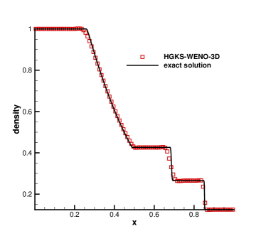
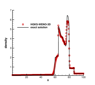
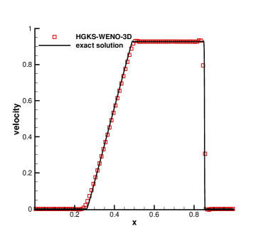
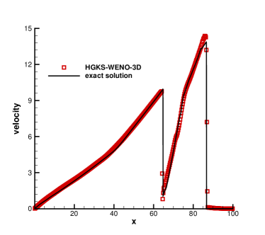
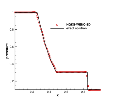
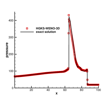
Figure 2: Riemann problem: the density, velocity and pressure distributions at $t=0.2$ for Sod problem (left), and the density, velocity and pressure distributions at $t=3.8$ for blast wave problem (right).

4.3 Riemann problem

In this case, one-dimensional Riemann problems are considered. The first one is the Sod problem, and the initial conditions are given by

$$(\rho,U,V,W,p)=\begin{cases}(1,0,0,0,1),\ \ \ \ &0\leq x<0.5,\\ (0.125,0,0,0,0.1),&0.5<x\leq 1.\end{cases}$$

The computational domain is $(x,y,z)\in[0,1]\times[0,0.1]\times[0,0.1]$, and the uniform mesh with $\Delta x=\Delta y=\Delta z=1/100$ is used. The non-reflected boundary condition is used in all directions. The second one is the Woodward-Colella blast wave problem, which is used to test the robustness of WENO reconstruction. The initial conditions are given as follows,

$$(\rho,U,V,W,p)=\left\{\begin{array}[]{ll}(1,0,0,0,1000),&0\leq x<10,\\ (1,0,0,0,0.01),&10\leq x<90,\\ (1,0,0,0,100),&90\leq x\leq 100.\end{array}\right.$$

The computational domain is $(x,y,z)\in[0,100]\times[0,10]\times[0,10]$, and the uniform mesh with $\Delta x=\Delta y=\Delta z=1/4$ is used. The reflected boundary condition is used in $x$ direction, and non-reflected boundary condition is used in $y$ and $z$ directions. The density, velocity, and pressure distributions for the current scheme and the exact solutions are presented in Fig.2 for the Sod problem at $t=0.2$ and for the blast wave problem at $t=3.8$ with $y=z=0$. The numerical results agree well with the exact solutions.

As an extension of the Sod problem, the spherically symmetric Sod problem is considered, and the initial conditions are given by

$$(\rho,U,V,W,p)=\begin{cases}(1,0,0,0,1),\ \ \ \ &0\leq\sqrt{x^{2}+y^{2}+z^{2}}<0.5,\\ (0.125,0,0,0,0.1),&0.5<\sqrt{x^{2}+y^{2}+z^{2}}\leq 1.\end{cases}$$

The computational domain is $(x,y,z)\in[0,1]\times[0,1]\times[0,1]$, and the uniform mesh with $\Delta x=\Delta y=\Delta z=1/100$ is used. The symmetric boundary condition is imposed on the plane with $x=0,y=0,z=0$, and the non-reflection boundary condition is imposed on the plane with $x=1,y=1,z=1$. The exact solution of spherically symmetric problem can be given by the following one-dimensional system with geometric source terms

$$\frac{\partial Q}{\partial t}+\frac{\partial F(Q)}{\partial r}=S(Q),$$

where

$$Q=\begin{pmatrix}\rho\\ \rho U\\ \rho E\\ \end{pmatrix},F(Q)=\begin{pmatrix}\rho U\\ \rho U^{2}+p\\ U(\rho E+p)\\ \end{pmatrix},S(Q)=-\frac{d-1}{r}\begin{pmatrix}\rho U\\ \rho U^{2}\\ U(\rho E+p)\\ \end{pmatrix}.$$

The radial direction is denoted by $r$, $U$ is the radial velocity, $d$ is the number of space dimensions. The density and pressure profiles along $y=z=0$ at $t=0.25$ are given in Fig.3. The current scheme also well resolves the wave profiles.

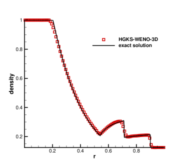
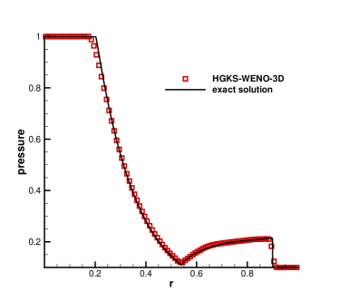
Figure 3: Riemann problem: the density and pressure distributions at $t=0.25$ for spherically symmetric Sod problem .

4.4 Sedov blast wave problem

This is a three-dimensional explosion problem to model blast wave from an energy deposited singular point. The initial density has a uniform unit distribution, and the pressure is $10^{-6}$ everywhere, except in the cell containing the origin. For this cell containing the origin, the pressure is defined as $p=(\gamma-1)\varepsilon_{0}/V$, where $\varepsilon_{0}=0.106384$ is the total amount of released energy and $V$ is the cell volume. The computation domain is $[0,1.2]\times[0,1.2]\times[0,1.2]$, and uniform meshes are used. Due to the singularity at the origin, a small CFL number $CFL=0.01$ is used. After 10 steps, a normal CFL number is used. The symmetric boundary condition is imposed on the plane with $x=0,y=0,z=0$, and the non-reflection boundary condition is imposed on the plane with $x=1.2,y=1.2,z=1.2$. The solution consists of a diverging infinite strength shock wave whose front is located at radius $r=1$ at $t=1$ [21]. The three-dimensional density and pressure distributions with $80\times 80\times 80$ cells at $t=1$ are presented in Fig.5. The density and pressure profiles long $y=z=0$ at $t=1$ with $20\times 20\times 20,40\times 40\times 40$ and $80\times 80\times 80$ cells are given in Fig.5. With the mesh refinement, the numerical solutions agree well with the exact solutions.

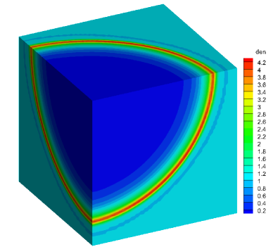
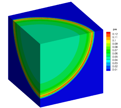
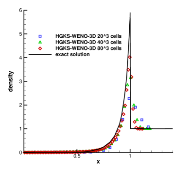
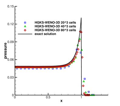
Figure 4: Sedov problem: the three-dimensional density and pressure distributions at $t=1$ with $80\times 80\times 80$ cells.

Figure 5: Sedov problem: the density and pressure profiles long $y=z=0$ at $t=1$.

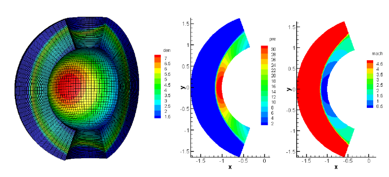
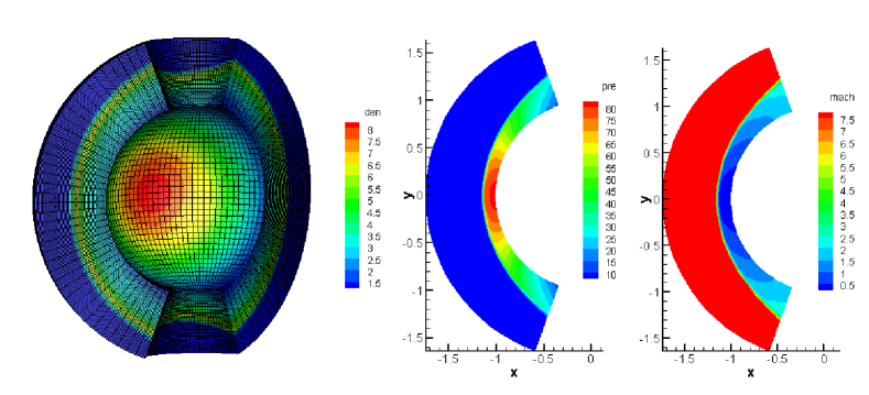
a b

Figure 6: Flow impinging on sphere: the mesh and density distribution, pressure and Mach number distribution at $\phi=0$ for $Ma=5$ (a) and $8$ (b).

4.5 Flow impinging on sphere

In this case, the inviscid hypersonic flows impinging on a unit sphere are tested to validate robustness of the current scheme with high Mach numbers. In the computation, a $50\times 40\times 40$ mesh is used, which represents the domain $[-1.75,-1]\times[-0.4\pi,0.4\pi]\times[0.1\pi,0.9\pi]$ in the spherical coordinate $(r,\phi,\theta)$. The mesh and density distributions in the whole domain, pressure and Mach number distributions at the plane with $\phi=0$ for the Mach number $Ma=5$ and $8$ are shown in Fig.6, where the shock is well captured by the current scheme and the carbuncle phenomenon does not appear.

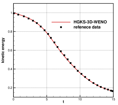
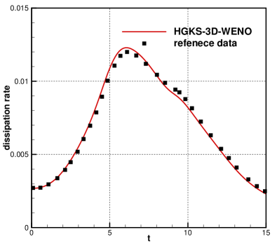
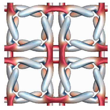
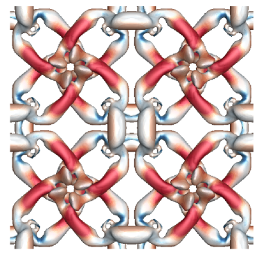
Figure 7: Taylor-Green Vortex: the time history of kinetic energy $E_{k}$ and dissipation rate $-\text{d}E_{k}/\text{d}t$.

Figure 8: Taylor-Green Vortex problem: the iso-surfaces of $Q$ criterion colored by velocity magnitude at time $t=5$ and $10$.

4.6 Taylor-Green Vortex

This problem is aimed at testing the performance of high-order methods on the direct numerical simulation of a three-dimensional periodic and transitional flow defined by a simple initial condition, i.e. the Taylor-Green vortex [6, 12]. With a uniform temperature field, the initial flow field is given by

$$u= V_{0}\sin(\frac{x}{L})\cos(\frac{y}{L})\cos(\frac{z}{L}),$$

$$v= -V_{0}\cos(\frac{x}{L})\sin(\frac{y}{L})\cos(\frac{z}{L}),$$

$$w= 0,$$

$$p= p_{0}+\frac{\rho_{0}V_{0}^{2}}{16}(\cos(\frac{2x}{L})+\cos(\frac{2y}{L}))(\cos(\frac{2z}{L})+2).$$

The fluid is then a perfect gas with $\gamma=1.4$ and the Prandtl number is $Pr=0.71$. Numerical simulations are conducted with two Reynolds numbers $Re=280$. The flow is computed within a periodic square box defined as $-\pi L\leq x,y,z\leq\pi L$. The characteristic convective time $t_{c}=L/V_{0}$. In the computation, $L=1,V_{0}=1,\rho_{0}=1$, and the Mach number takes $M_{0}=V_{0}/c_{0}=0.1$, where $c_{0}$ is the sound speed. The volume-averaged kinetic energy can be computed from the flow as it evolves in time, which is expressed as

$$E_{k}=\frac{1}{\rho_{0}\Omega}\int_{\Omega}\frac{1}{2}\rho\bm{u}\cdot\bm{u}\text{d}\Omega,$$

where $\Omega$ is the volume of the computational domain, and the dissipation rate of the kinetic energy is given by

$$\varepsilon_{k}=-\frac{\text{d}E_{k}}{\text{d}t}.$$

The numerical results with $192\times 192\times 192$ mesh points for the normalized volume-averaged kinetic energy and dissipation rate are presented in Fig.8, which agree well with the data in [36]. The iso-surfaces of $Q$ criterions colored by velocity magnitude at $t=5$ and $10$ are shown in Fig.8. The complex structures can be well captured by the current scheme.

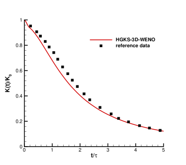
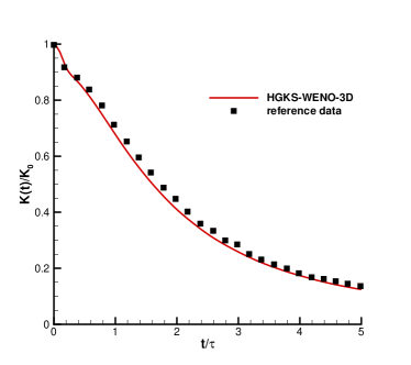
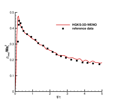
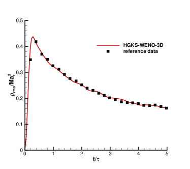
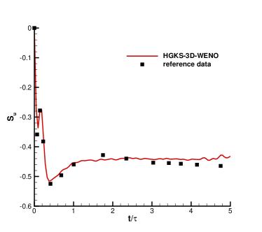
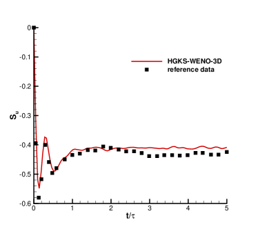
Figure 9: Compressible isotropic turbulence: time history of $\rho_{rms}/Ma_{t}^{2}$, $K/K_{0}$, $S_{u}(t)$ with respect to $t/\tau$ and Mach number distribution with $Ma_{t}=0.3$ (left) and $0.5$ (right).

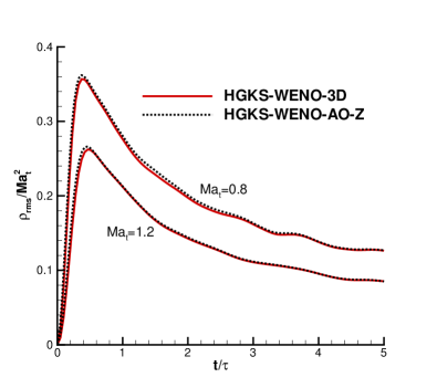
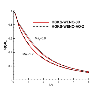
Figure 10: Compressible isotropic turbulence: time history of $\rho_{rms}/Ma_{t}^{2}$ and $K/K_{0}$ with respect to $t/\tau$ with $Ma_{t}=0.8$ and $1.2$.

4.7 Compressible isotropic turbulence

The compressible isotropic turbulence is regarded as one of cornerstones to elucidate the effects of compressibility for compressible turbulence[31, 37]. The flow is computed within a square box defined as $-\pi\leq x,y,z\leq\pi$, and the periodic boundary conditions are used in all directions for all the flow variables. A divergence-free random initial velocity field $\bm{u}_{0}$ is generated for a given spectrum with a specified root mean square $u_{rms}$ as follows

$$u_{rms}=<\frac{\bm{u}\cdot\bm{u}}{3}>^{1/2},$$

where $<...>$ is a volume average over the whole computational domain. The specified spectrum for velocity is given by

$$E(\kappa)=A_{0}\kappa^{4}\exp(-2\kappa^{2}/\kappa_{0}^{2}),$$

where $\kappa$ is the wave number, $\kappa_{0}$ is the wave number at spectrum peaks, and $A_{0}$ is a constant chosen to get a specified initial kinetic energy. With current initial strategy, the initial ensemble turbulent kinetic energy $K_{0}$, ensemble enstrophy $\Omega_{0}$, ensemble dissipation rate $\varepsilon_{0}$, large-eddy-turnover time $\tau_{t_{0}}$, Kolmogorov length scale $\eta_{0}$, and the Kolmogorov time scale $\tau_{0}$ are given as

$$K_{0}= \frac{3A_{0}}{64}\sqrt{2\pi}\kappa_{0}^{5},~{}\Omega_{0}=\frac{15A_{0}}{256}\sqrt{2\pi}\kappa_{0}^{7},~{}\tau_{t_{0}}=\sqrt{\frac{32}{A_{0}}}(2\pi)^{1/4}\kappa_{0}^{-7/2},$$

$$\varepsilon_{0}=\frac{2\mu_{0}\Omega_{0}}{\rho_{0}},~{}\eta_{0}=(\nu_{0}^{3}/\varepsilon_{0})^{1/4},~{}\tau_{0}=(\nu_{0}/\varepsilon_{0})^{1/2}.$$

The evolution of this system is dominated by the initial thermodynamic quantities and two dimensionless parameters, i.e. the initial Taylor microscale Reynolds number and turbulent Mach number

$$Re_{\lambda}= \frac{<\rho>u_{rms}\lambda}{<\mu>}=\frac{(2\pi)^{1/4}}{4}\frac{\rho_{0}}{\mu_{0}}\sqrt{2A_{0}}k_{0}^{3/2},$$

$$Ma_{t}=\frac{\sqrt{3}u_{rms}}{<c_{s}>}=\frac{\sqrt{3}u_{rms}}{\sqrt{\gamma T_{0}}},$$

where $\lambda$ is Taylor microscale

$$\lambda^{2}=\frac{u_{rms}^{2}}{<(\partial_{x}u)^{2}>}.$$

The dynamic viscosity is determined by

$$\mu=\mu_{0}\big{(}\frac{T}{T_{0}}\big{)}^{0.76},$$

where $\mu_{0}$ and $T_{0}$ can be determined from $Re_{\lambda}$ and $Ma_{t}$ with initialized $u_{rms}$ and $\rho_{0}=1$.

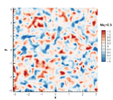
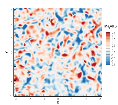
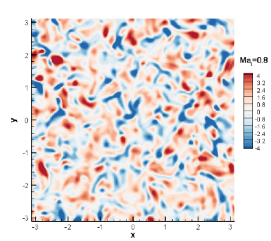
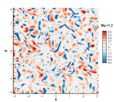
Figure 11: Compressible isotropic turbulence: the contours of dilation $\theta=\nabla\cdot\bm{u}$ at $t/\tau=1$ with $Ma_{t}=0.3,0.5,0.8$ and $1.2$.

High-order compact finite difference method [22] has been widely utilized in the simulation of isotropic compressible turbulence with moderate turbulent Mach number ($Ma_{t}\leq 0.8$). However, when simulating the turbulent in supersonic regime ($Ma_{t}\geq 0.8$), the above scheme fails to capture strong shocklets and suffers from numerical instability. However, the current HGKS scheme will be tested at a wide range turbulent Mach numbers. In the computation, $A_{0}=1.3\times 10^{-4},k_{0}=8$, $Re_{\lambda}=72$ and the uniform meshes with $128^{3}$ cells are used. The compressible isotropic turbulent flows in nonlinear subsonic regime with $Ma_{t}=0.3$ and $0.5$ are tested firstly. The time history of normalized kinetic energy $K(t)/K_{0}$, normalized root-mean-square of density fluctuation $\rho_{rms}(t)/Ma_{t}^{2}$ and skewness factor $S_{u}(t)$ with respect to $t/\tau$ are given in Fig.9. The numerical results agree well with the reference data [31]. With fixed initial $Re_{\lambda}=72$ and $128^{3}$ cells, the cases with $Ma_{t}=0.8$ and $1.2$ are tested as well, which go up to the supersonic turbulent Mach number. The time histories of normalized kinetic energy $K(t)/K_{0}$ and normalized root-mean-square of density fluctuation $\rho_{rms}(t)/Ma_{t}^{2}$ at $t/\tau=1$ are given in Fig.10 as well. With the increase of $Ma_{t}$, the dynamic viscosity increases and the kinetic energy gets dissipated more rapidly. As comparison, the numerical results with fifth-order WENO-Z scheme are given as well. More studies of compressible isotropic turbulence can be referred in [7]. The contours of dilation $\theta=\nabla\cdot\bm{u}$ for $Ma_{t}=0.3,0.5,0.8$ and $1.2$ are given in Fig.11, which shows very different behavior between the compression motion and expansion motion. With the increase of $Ma_{t}$, the compression regions, i.e. shocklets behave in the shape of narrow and long “ribbon”. In addition, the strong compression regions are close to several regions of high expansion. Compared the case with $Ma_{t}=0.3$ in subsonic regime, the supersonic case with $Ma_{t}=1.2$ contains much more crisp shocklets, which pose much greater challenge for high-order schemes when implementing DNS for isotropic turbulence in supersonic regime, which validate the robustness for the challenging compressible turbulence problems.

5 Conclusion

In this paper, with the WENO-AO reconstruction an efficient and simple third-order gas-kinetic scheme is developed for the three-dimensional Euler and Navier-Stokes equations. In the classical WENO scheme, choosing sub-stencils from big stencil and solving linear weights at Gaussian quadrature points would make the reconstruction complicated, especially for three-dimensional flows. To overcome the drawback, the WENO-AO strategy is adopted. Based on the candidate stencils, the quadratic polynomial for big stencil and linear polynomials for sub-stencils are constructed. The spatial independent linear weights are used, which have fixed values and become positive. With the smooth indicator, the nonlinear weights can be constructed. Through particle colliding procedure, the point-value and slopes for equilibrium part are obtained directly from the initial reconstruction of the non-equilibrium state, an extra reconstruction for the equilibrium state in the classical HGKS is avoided. Taken the grid velocity into account, such scheme can be also extended to the moving-mesh computation. For the mesh with non-coplanar vertexes, which is commonly generated in the moving-mesh computation, the trilinear interpolation is used to parameterize the hexahedron, and the bilinear interpolation is used to parameterize the interface of hexahedron. Numerical results are provided to illustrate the good performance of the WENO schemes from the smooth inviscid flows to the supersonic turbulent flows. In the future, the extension to unstructured meshes will be developed.

References

- [1] R. Abgrall, On essentially non-oscillatory schemes on unstructured meshes: Analysis and implementation, J. Comput. Phys. 114 (1994) 45-58.
- [2] D.S. Balsara, S. Garain, C.W. Shu. An efficient class of WENO schemes with adaptive order. Journal of Computational Physics, 326 (2016) 780 C804.
- [3] M. Ben-Artzi, J. Li, Hyperbolic conservation laws: Riemann invariants and the generalized Riemann problem, Numerische Mathematik. 106 (2007) 369-425.
- [4] P.L. Bhatnagar, E.P. Gross, M. Krook, A Model for Collision Processes in Gases I: Small Amplitude Processes in Charged and Neutral One-Component Systems, Phys. Rev. 94 (1954) 511-525.
- [5] R. Borges, M. Carmona, B. Costa, W. S. Don, An improved weighted essentially non-oscillatory scheme for hyperbolic conservation laws, J. Comput. Phys. 227 (2008) 3191-3211.
- [6] J. R. Bull, A. Jameson, Simulation of the compressible Taylor-Green vortex using high-order flux reconstruction schemes, AIAA 2014-3210.
- [7] G.Y. Cao, L. Pan, K. Xu, Three dimensional high-order gas-kinetic scheme for supersonic isotropic turbulence I: criterion for direct numerical simulation, Computers Fluids 192 (2019) 104273.
- [8] S. Chapman, T.G. Cowling, The Mathematical theory of non-uniform gases, third edition, Cambridge University Press, (1990).
- [9] B. Cockburn, C.W. Shu, TVB Runge-Kutta local projection discontinuous Galerkin finite element method for conservation laws II: general framework, Mathematics of Computation, 52 (1989) 411-435.
- [10] B. Cockburn, C.W. Shu, The Runge-Kutta discontinuous Galerkin method for conservation laws V: multidimensional systems, J. Comput. Phys. 141 (1998) 199-224.
- [11] M. Dumbser, M. Kaser, Arbitrary high order non-oscillatory finite volume schemes on unstructured meshes for linear hyperbolic systems, J. Comput. Phys. 221 (2007) 693 C723.
- [12] J. Debonis, Solutions of the Taylor-Green vortex problem using high-resolution explicit finite difference methods, AIAA Paper (2013) 2013-0382.
- [13] Z.F. Du, J.Q. Li, A Hermite WENO reconstruction for fourth order temporal accurate schemes based on the GRP solver for hyperbolic conservation laws, J. Comput. Phys. 355 (2018) 385-396.
- [14] S. Gottlieb, C.W. Shu, Total variation diminishing Runge-Tutta schemes, Mathematics of computation, 67 (1998) 73-85.
- [15] A. Harten, B. Engquist, S. Osher and S. R. Chakravarthy, Uniformly high order accurate essentially non-oscillatory schemes, III. J. Comput. Phys. 71 (1987) 231-303.
- [16] A. K. Henrick, T. D. Aslam, J. M. Powers, Mapped weighted essentially non-oscillatory schemes: achieving optimal order near critical points, J. Comput. Phys. 207 (2005) 542-567.
- [17] C. Hu, C.W. Shu, Weighted essentially non-oscillatory schemes on triangular meshes, J. Comput. Phys. 150 (1999) 97-127.
- [18] X. Ji, L. Pan, W. Shyy, K. Xu, A compact fourth-order gas-kinetic scheme for the Euler and Navier-Stokes equations, J. Comput. Phys. 372 (2018) 446-472.
- [19] X. Ji, K. Xu, Performance Enhancement for High-order Gas-kinetic Scheme Based on WENO-adaptive-order Reconstruction, arXiv:1905.08489v1.
- [20] G.S. Jiang, C. W. Shu, Efficient implementation of weighted ENO schemes, J. Comput. Phys. 126 (1996) 202-228.
- [21] J.R. Kamm, F.X. Timmes, On efficient generation of numerically robust Sedov solutions, Technical Report LA-UR-07-2849, Los Alamos National Laboratory, (2007).
- [22] S.K. Lele, Compact finite difference schemes with spectral-like resolution, J. Comput. Phys. 103 (1992) 16-42.
- [23] J.Q. Li, Z.F. Du, A two-stage fourth order time-accurate discretization for Lax-Wendroff type flow solvers I. hyperbolic conservation laws, SIAM J. Sci. Computing, 38 (2016) 3046-3069.
- [24] Q.B. Li, K. Xu, S. Fu, A high-order gas-kinetic Navier-Stokes flow solver, J. Comput. Phys. 229 (2010) 6715-6731.
- [25] X.D. Liu, S. Osher, T. Chan, Weighted essentially non-oscillatory schemes, J. Comput. Phys. 115 (1994) 200-212.
- [26] N. Liu, H.Z. Tang, A high-order accurate gas-kinetic scheme for one- and two-dimensional flow simulation, Commun. Comput. Phys. 15 (2014) 911-943.
- [27] L. Pan, F.X. Zhao, K. Xu, High-order ALE gas-kinetic scheme with unstructured WENO reconstruction, arXiv:1905.07837.
- [28] L. Pan, K. Xu, Q.B. Li, J.Q. Li, An efficient and accurate two-stage fourth-order gas-kinetic scheme for the Navier-Stokes equations, J. Comput. Phys. 326 (2016), 197-221.
- [29] L. Pan, K. Xu, Two-stage fourth-order gas-kinetic scheme for three-dimensional Euler and Navier-Stokes solutions, Int. J. Comput. Fluid Dynamics, 32 (2018) 395-411.
- [30] L. Pan, F.X. Zhao, K. Xu, High-order ALE gas-kinetic scheme with unstructured WENO reconstruction, arXiv:1905.07837v1
- [31] R. Samtaney, D.I. Pullin, B. Kosovic, Direct numerical simulation of decaying compressible turbulence and shocklet statistics. Physiscs of Fluids 13 (2001) 1415-1430.
- [32] J. Shi, C. Hu, C.W. Shu, A technique of treating negative weights in WENO schemes, J. Comput. Phys. 175 (2002) 108-127.
- [33] C.W. Shu, S. Osher, Efficient implementation of essentially nonoscillatory shock-capturing schemes II, J. Comput. Phys. 83 (1989) 32-78.
- [34] P. Thomas, C. Lombard, Geometric conservation law and its application to flow computations on moving grids, AIAA J. 17 (1979) 1030-1037.
- [35] E.F. Toro, Riemann Solvers and Numerical Methods for Fluid Dynamics, Third Edition, Springer (2009).
- [36] L. Wang, W. K. Anderson, T. Erwin, S. Kapadia, High-order discontinuous Galerkin method for computation of turbulent flows, AIAA Journal 53 (2015) 1157-1171.
- [37] J.C. Wang, L.P. Wang, Z.L. Xiao, Y. Shi, S.Y. Chen, A hybrid numerical simulation of isotropic compressible turbulence, J. Comput. Phys. 229 (2010) 5257-5279.
- [38] K. Xu, Direct modeling for computational fluid dynamics: construction and application of unfied gas kinetic schemes, World Scientific (2015).
- [39] K. Xu, A gas-kinetic BGK scheme for the Navier-Stokes equations and its connection with artificial dissipation and Godunov method, J. Comput. Phys. 171 (2001) 289-335.
- [40] F.X. Zhao, L. Pan, S.H. Wang, Weighted essentially non-oscillatory scheme on unstructured quadrilateral and triangular meshes for hyperbolic conservation laws, J. Comput. Phys. 374 (2018) 605-624.
- [41] F.X. Zhao, X. Ji, W. Shyy, K. Xu, Compact higher-order gas-kinetic schemes with spectral-like resolution for compressible flow simulations, Advances in Aerodynamics 1:13 (2019).
- [42] J. Zhu, J.X. Qiu, A new fifth order finite difference weno scheme for solving hyperbolic conservation laws. J. Comput. Phys. 318 (2016) 110-121.
- [43] J. Zhu, J.X. Qiu, New finite volume weighted essentially non-oscillatory scheme on triangular meshes, SIAM J. Sci. Computing, 40 (2018) 903-928.