A Non-commutative Bilinear Model for Answering Path Queries in Knowledge Graphs

Abstract

Bilinear diagonal models for knowledge graph embedding (KGE), such as DistMult and ComplEx, balance expressiveness and computational efficiency by representing relations as diagonal matrices. Although they perform well in predicting atomic relations, composite relations (relation paths) cannot be modeled naturally by the product of relation matrices, as the product of diagonal matrices is commutative and hence invariant with the order of relations. In this paper, we propose a new bilinear KGE model, called BlockHolE, based on block circulant matrices. In BlockHolE, relation matrices can be non-commutative, allowing composite relations to be modeled by matrix product. The model is parameterized in a way that covers a spectrum ranging from diagonal to full relation matrices. A fast computation technique is developed on the basis of the duality of the Fourier transform of circulant matrices.

1 Introduction

Large-scale knowledge graphs Nickel et al. (2016a) are indispensable resources for knowledge-intensive applications such as question answering, dialog systems, and distantly supervised relation extraction. A knowledge graph is a collection of triplets $(s,r,o)$ representing the fact that (binary) relation $r$ holds between subject entity $s$ and object entity $o$. Although efforts continue to enrich existing knowledge graphs with more facts, many facts are still missing Nickel et al. (2016a). Knowledge graph completion (KGC) aims to automatically detect missing facts in an incomplete knowledge graph, and has become an active field of research in recent years.

Figure 1: (a) A knowledge graph and (b,c) two relation paths starting from William.

Knowledge graph embedding (KGE) is a promising approach to KGC. It embeds entities and relations in vector space, and defines a scoring function $\phi(s,r,o)$ to evaluate the degree of factuality of a given triplet $(s,r,o)$ in terms of vector operations.

Bilinear KGE models are a popular choice for a scoring function, along with those based on translation and neural networks. RESCAL Nickel et al. (2011) adopts a generic bilinear form as the scoring function, given by $\phi_{\text{RESCAL}}(s,r,o)=\boldsymbol{\mathbf{e}}_{s}^{\mathrm{T}}\boldsymbol{\mathbf{R}}_{r}\boldsymbol{\mathbf{e}}_{o}$. In this formula, $\boldsymbol{\mathbf{e}}_{s},\boldsymbol{\mathbf{e}}_{o}$ are the $n$-dimensional vector embeddings of entities $s$ and $o$, respectively, and $\boldsymbol{\mathbf{R}}_{r}$ is the $n\times n$ matrix embedding of relation $r$. Some of the more recent models have constrained the relation matrices to be diagonal. DistMult Yang et al. (2015) and ComplEx Trouillon et al. (2016) are two such diagonal models. HolE Nickel et al. (2016b) does not use diagonal relation matrices, but has been shown Hayashi and Shimbo (2017) to be isomorphic to ComplEx. These models have a smaller number of parameters than RESCAL, making them less prone to overfitting, and the performance is usually better.

While all these models were designed with a specific task of KGC in mind, i.e., computing the factuality of triplets, another important task on knowledge graphs was pursued by Guu et al. (2015) and Lin et al. (2015). This latter task, called path query answering (path QA), is to answer composite queries that consist of a cascade of relations, as opposed to an atomic relation. See Figure 1 for instance. A query “Is Beatrice a child of a paternal uncle of William?” can be answered by predicting the truth value of the triplet (William, fatherOf^-1/brotherOf/fatherOf, Beatrice) where fatherOf^-1/brotherOf/fatherOf is a binary relation not present in the knowledge graph as a relation (edge) label but is composed of a cascade of three atomic relations. Composite queries are also called path queries, as they can be represented as paths in a knowledge graph; see, e.g., the blue line in Figure 1(a). Notice however that some of the edges in the path may be missing due to the incompleteness of the knowledge graph; even in such circumstances, the model must ideally be able to answer path queries correctly.

Guu et al. (2015) extended the existing KGE approaches to path QA. For example, to answer a general path query $(s,r_{1}/\dots/r_{k},o)$ with RESCAL, a composite relation $r_{1}/\cdots/r_{k}$ is modeled by matrix product $\boldsymbol{\mathbf{R}}_{r_{1}}\cdots\boldsymbol{\mathbf{R}}_{r_{k}}$, and the score for the given query is modeled by $\boldsymbol{\mathbf{e}}_{s}^{\mathrm{T}}\boldsymbol{\mathbf{R}}_{r_{1}}\cdots\boldsymbol{\mathbf{R}}_{r_{k}}\boldsymbol{\mathbf{e}}_{o}$. This formulation is also applicable to DistMult and ComplEx, which use diagonal relation matrices. In diagonalized models, however, relation matrices are commutative, in the sense that $\boldsymbol{\mathbf{R}}_{r}\boldsymbol{\mathbf{R}}_{r^{\prime}}=\boldsymbol{\mathbf{R}}_{r^{\prime}}\boldsymbol{\mathbf{R}}_{r}$ for any pair of relations $r,r^{\prime}$.

Commutativity of relation matrices was not recognized as an issue in the past research because the main focus was on predicting the truth value of atomic triplets. However, when path queries are concerned, commutativity poses a problem. Consider, for example, a relation sequence

fatherOf^-1/brotherOf/fatherOf

and its permutation

$$\text{brotherOf/fatherOf${}^{-1}$/fatherOf}.$$

Although these are two distinct paths (cf. Figure 1(b, c)), in bilinear models with commutative relation matrices, they are represented by the same product of relation matrices, which thereby makes the truth values of these permutated queries indistinguishable by their scores.

Drawing on the observation above, this paper proposes a new KGE model called BlockHolE, wherein relations are represented by block circulant matrices. This makes relation matrices non-commutative, and thus it does not suffer from the issues arising from commutativity, yet in general manages to reduce the number of parameters compared with RESCAL. It can be interpreted as a generalization of HolE and ComplEx, and also subsumes RESCAL as an extreme case. We report experimental results in both path and atomic QA tasks.

2 Notation and preliminaries

Symbol	Description
$\mathbb{R},\mathbb{C}$	sets of real/complex numbers
$[\boldsymbol{\mathbf{v}}]_{j}$	$j$th component of vector $\boldsymbol{\mathbf{v}}$
$[\boldsymbol{\mathbf{M}}]_{jk}$	$(j,k)$-component of matrix $\boldsymbol{\mathbf{M}}$
$\boldsymbol{\mathbf{M}}^{\text{T}}$	transpose of $\boldsymbol{\mathbf{M}}$
$\overline{\boldsymbol{\mathbf{M}}}$	conjugate of $\boldsymbol{\mathbf{M}}$
$\odot$	componentwise (Hadamard) product
	circular convolution
$\star$	circular correlation
$\mathop{\text{Re}}(x)$	real part of complex number $x$
$\mathop{\text{diag}}(\boldsymbol{\mathbf{v}})$	diagonal matrix with main diagonal $\boldsymbol{\mathbf{v}}$
$\text{circ}(\boldsymbol{\mathbf{v}})$	circulant matrix determined by $\boldsymbol{\mathbf{v}}$
$\langle\boldsymbol{\mathbf{x}},\boldsymbol{\mathbf{y}},\boldsymbol{\mathbf{z}}\rangle$	sum of the componentwise products of $\boldsymbol{\mathbf{x}},\boldsymbol{\mathbf{y}},\boldsymbol{\mathbf{z}}$
$\boldsymbol{\mathbf{F}}$	discrete Fourier matrix
$\mathcal{E}$	set of entities
$\mathcal{R}$	set of relations
$\mathcal{F}$	set of observed facts (triplets)
$\mathcal{F}^{*}$	set of ground truth facts
$\mathcal{G}(\mathcal{F})$	Knowledge graph induced by facts $\mathcal{F}$

Table 1: List of symbols. See Secs. 2 and 3 for detail.

We first introduce symbols and notation used in this paper, followed by some preliminaries on circulant matrices, circular convolution, correlation, and Fourier transform. The summary of symbols can be found in Table 1.

Let $\mathbb{R}$ be the set of reals, and $\mathbb{C}$ be the set of complex numbers. Let $[\boldsymbol{\mathbf{v}}]_{j}$ denote the $j$th component of vector $\boldsymbol{\mathbf{v}}$, and let $[\boldsymbol{\mathbf{M}}]_{jk}$ the $(j,k)$ element of matrix $\boldsymbol{\mathbf{M}}$. For a complex number $z$, vector $\boldsymbol{\mathbf{z}}$, and matrix $\boldsymbol{\mathbf{Z}}$, let $\overline{z}$, $\overline{\boldsymbol{\mathbf{z}}}$, and $\overline{\boldsymbol{\mathbf{Z}}}$ denote their complex conjugate, respectively.

Let $\boldsymbol{\mathbf{x}}$, $\boldsymbol{\mathbf{y}}$, and $\boldsymbol{\mathbf{z}}$ be $n$-dimensional (real or complex) vectors. Let $\mathop{\text{diag}}(\boldsymbol{\mathbf{x}})$ denote an $n\times n$ diagonal matrix with the main diagonal components given by $\boldsymbol{\mathbf{x}}$. We write $\boldsymbol{\mathbf{x}}\odot\boldsymbol{\mathbf{y}}$ to denote the componentwise product of $\boldsymbol{\mathbf{x}}$ and $\boldsymbol{\mathbf{y}}$; i.e., $\boldsymbol{\mathbf{x}}\odot\boldsymbol{\mathbf{y}}=\mathop{\text{diag}}(\boldsymbol{\mathbf{x}})\boldsymbol{\mathbf{y}}$, or $[\boldsymbol{\mathbf{x}}\odot\boldsymbol{\mathbf{y}}]_{i}=[\boldsymbol{\mathbf{x}}]_{i}[\boldsymbol{\mathbf{y}}]_{i}$, $i=1,\dots,n$. We also write $\langle\boldsymbol{\mathbf{x}},\boldsymbol{\mathbf{y}},\boldsymbol{\mathbf{z}}\rangle=\boldsymbol{\mathbf{x}}^{\mathrm{T}}\mathop{\text{diag}}(\boldsymbol{\mathbf{y}})\boldsymbol{\mathbf{z}}=\sum_{i=1}^{n}[\boldsymbol{\mathbf{x}}]_{i}[\boldsymbol{\mathbf{y}}]_{i}[\boldsymbol{\mathbf{z}}]_{i}$.

For $n$-dimensional real vectors $\boldsymbol{\mathbf{x}},\boldsymbol{\mathbf{y}}\in\mathbb{R}^{n}$, $\boldsymbol{\mathbf{x}}*\boldsymbol{\mathbf{y}}$ and $\boldsymbol{\mathbf{x}}\star\boldsymbol{\mathbf{y}}$ denote circular convolution and circular correlation, respectively defined by

$$[\boldsymbol{\mathbf{x}}*\boldsymbol{\mathbf{y}}]_{i} =\sum_{j=1}^{n}[\boldsymbol{\mathbf{x}}]_{i-j+1}[\boldsymbol{\mathbf{y}}]_{j},$$

$$[\boldsymbol{\mathbf{x}}\star\boldsymbol{\mathbf{y}}]_{i} =\sum_{j=1}^{n}[\boldsymbol{\mathbf{x}}]_{j-i+1}[\boldsymbol{\mathbf{y}}]_{j},\quad i=1,\dots,n,$$

where vector indices that do not fall in the range $1,\ldots,n$ must be interpreted by $0=n,-1=n-1,\dots,-n+1=1$.

For $n$-dimensional real vector $\boldsymbol{\mathbf{v}}\in\mathbb{R}^{n}$, let

$$\mathop{\text{circ}}(\boldsymbol{\mathbf{v}})=\begin{bmatrix}[\boldsymbol{\mathbf{v}}]_{1}&[\boldsymbol{\mathbf{v}}]_{n}&\dots&[\boldsymbol{\mathbf{v}}]_{3}&[\boldsymbol{\mathbf{v}}]_{2}\\ [\boldsymbol{\mathbf{v}}]_{2}&[\boldsymbol{\mathbf{v}}]_{1}&[\boldsymbol{\mathbf{v}}]_{n}&&[\boldsymbol{\mathbf{v}}]_{3}\\ \vdots&[\boldsymbol{\mathbf{v}}]_{2}&[\boldsymbol{\mathbf{v}}]_{1}&\ddots&\vdots\\ [\boldsymbol{\mathbf{v}}]_{n-1}&&\ddots&\ddots&[\boldsymbol{\mathbf{v}}]_{n}\\ [\boldsymbol{\mathbf{v}}]_{n}&[\boldsymbol{\mathbf{v}}]_{n-1}&\dots&[\boldsymbol{\mathbf{v}}]_{2}&[\boldsymbol{\mathbf{v}}]_{1}\end{bmatrix}$$

be an operation that converts a vector $\boldsymbol{\mathbf{v}}$ to a circulant matrix of size $n\times n$.

A circulant matrix $\mathop{\text{circ}}(\boldsymbol{\mathbf{v}})\in\mathbb{R}^{n\times n}$ can be diagonalized as $\mathop{\text{circ}}(\boldsymbol{\mathbf{v}})=\boldsymbol{\mathbf{F}}^{\mathrm{-1}}\mathop{\text{diag}}(\boldsymbol{\mathbf{F}}\boldsymbol{\mathbf{v}})\boldsymbol{\mathbf{F}}$, where $\boldsymbol{\mathbf{F}}\in\mathbb{C}^{n\times n}$ is the discrete Fourier matrix of order $n$. Also, circular convolution and correlation can be written in terms of $\mathop{\text{circ}}(\cdot)$: $\boldsymbol{\mathbf{x}}*\boldsymbol{\mathbf{y}}=\mathop{\text{circ}}(\boldsymbol{\mathbf{x}})\boldsymbol{\mathbf{y}}$, and $\boldsymbol{\mathbf{x}}\star\boldsymbol{\mathbf{y}}=\mathop{\text{circ}}(\boldsymbol{\mathbf{x}})^{\mathrm{T}}\boldsymbol{\mathbf{y}}$. It follows that

$$\boldsymbol{\mathbf{x}}*\boldsymbol{\mathbf{y}} =\boldsymbol{\mathbf{F}}^{\mathrm{-1}}(\boldsymbol{\mathbf{F}}\boldsymbol{\mathbf{x}}\odot\boldsymbol{\mathbf{F}}\boldsymbol{\mathbf{y}}),$$ (1)

$$\boldsymbol{\mathbf{x}}\star\boldsymbol{\mathbf{y}} =\boldsymbol{\mathbf{F}}^{\mathrm{-1}}(\overline{\boldsymbol{\mathbf{F}}\boldsymbol{\mathbf{x}}}\odot\boldsymbol{\mathbf{F}}\boldsymbol{\mathbf{y}}).$$ (2)

These equations imply that circular convolution and correlation can be computed in time $O(n\log n)$ using the fast Fourier transform (FFT).

3 Knowledge graph embedding using bilinear maps

A knowledge graph is a labeled multigraph $(\mathcal{E},\mathcal{R},\mathcal{F})$, where $\mathcal{E}$ is the set of entities (or vertices), $\mathcal{R}$ is the set of relation labels (or edge labels), and $\mathcal{F}\subset\mathcal{E}\times\mathcal{R}\times\mathcal{E}$ defines the observed instances of binary relations over entities (or labeled edges). An item $(s,r,o)\in\mathcal{E}\times\mathcal{R}\times\mathcal{E}$ is called a triplet, with $s$ and $o$ called its subject and object, respectively. For every entity in $e\in\mathcal{E}$, it is assumed that $\mathcal{F}$ contains at least one triplet $(s,r,o)$ with $s=e$ or $o=e$; likewise, for every relation in $r\in\mathcal{R}$, $\mathcal{F}$ is assumed to contain at least one triplet $(s,r,o)$. Because $\mathcal{F}$ determines the sets $\mathcal{E}$ and $\mathcal{R}$ of entities and relations, we write $\mathcal{G}(\mathcal{F})$ to denote the knowledge graph $(\mathcal{E},\mathcal{R},\mathcal{F})$ determined by $\mathcal{F}$.

Aside from observed triplets $\mathcal{F}$, we also assume the presence of a set $\mathcal{F}^{*}\subset\mathcal{E}\times\mathcal{R}\times\mathcal{E}$ of (ground truth) facts, which is a strict superset of $\mathcal{F}$, i.e., $\mathcal{F}\subset\mathcal{F}^{*}$. Thus, $\mathcal{F}^{*}$ is not fully observable.

3.1 Knowledge graph completion

Knowledge graph completion (KGC) is the task of identifying the set of ground truth facts $\mathcal{F}^{*}$ from observed facts $\mathcal{F}\subset\mathcal{F}^{*}$ (or equivalently, $\mathcal{G}(\mathcal{F}^{*})$ from $\mathcal{G}(\mathcal{F})$).

A popular approach to KGC is to design a scoring function $\phi(s,r,o)$ quantifying how likely a triplet $(s,r,o)$ is true. This scoring function is learned from the observed triplets $\mathcal{F}$, in a way that it generalizes well to unobserved triplets $\mathcal{F}^{*}\backslash\mathcal{F}$; i.e., the score must be high for both observed and unobserved facts, and it must be low for nonfactual triplets.

In knowledge graph embedding (KGE)–based approaches to KGC, the scoring function $\phi(s,r,o)$ is defined in terms of the embeddings of entities and relations; i.e., $s$, $r$, and $o$ are embedded as objects in a vector space, and $\phi$ is defined in terms of some operations over these objects.

3.2 Bilinear models for knowledge graph embedding

Below, we describe some of the popular KGE models that use bilinear maps to define scoring functions.

3.2.1 RESCAL

RESCAL Nickel et al. (2011) provides the most general form of bilinear scoring function.

$$\phi_{\text{RESCAL}}(s,r,o)=\boldsymbol{\mathbf{e}}_{s}^{\mathrm{T}}\boldsymbol{\mathbf{R}}_{r}\boldsymbol{\mathbf{e}}_{o},$$ (3)

where $\boldsymbol{\mathbf{e}}_{s},\boldsymbol{\mathbf{e}}_{o}\in\mathbb{R}^{n}$ are the vector embeddings of entities $s$ and $o$, respectively, and $\boldsymbol{\mathbf{R}}_{r}\in\mathbb{R}^{n\times n}$ is the matrix representing relation $r$. Thus, $n^{2}$ parameters are required per relation, which is not only a computational burden but also the cause of overfitting during training Kazemi and Poole (2018).

3.2.2 DistMult

DistMult Yang et al. (2015) is a model obtained by restricting the relation matrices $\boldsymbol{\mathbf{R}}_{r}$ of RESCAL to diagonal; i.e., $\boldsymbol{\mathbf{R}}_{r}=\mathop{\text{diag}}(\boldsymbol{\mathbf{w}}_{r})$, $\boldsymbol{\mathbf{w}}_{r}\in\mathbb{R}^{n}$. The scoring function is thus

$$\phi_{\text{DistMult}}(s,r,o) ={\boldsymbol{\mathbf{e}}_{s}}^{\mathrm{T}}\mathop{\text{diag}}(\boldsymbol{\mathbf{w}}_{r})\boldsymbol{\mathbf{e}}_{o}$$

$$=\langle\boldsymbol{\mathbf{w}}_{r},\boldsymbol{\mathbf{e}}_{s},\boldsymbol{\mathbf{e}}_{o}\rangle.$$ (4)

Although the number of parameters is reduced considerably, the scoring function (4) is symmetric with respect to the entities, i.e., $\phi_{\text{DistMult}}(s,r,o)=\phi_{\text{DistMult}}(o,r,s)$. This is a severe limitation because most real-world relations are non-symmetric.

3.2.3 ComplEx: Complex embedding

The complex embedding (ComplEx) Trouillon et al. (2016) represents entities and relations as $n$-dimensional vectors as in DistMult, but their components are complex-valued.

The scoring function of ComplEx is given by

$$\phi_{\text{ComplEx}}(s,r,o) =\mathop{\text{Re}}({\boldsymbol{\mathbf{e}}_{s}}^{\mathrm{T}}\mathop{\text{diag}}(\boldsymbol{\mathbf{w}}_{r})\overline{\boldsymbol{\mathbf{e}}_{o}})$$

$$=\mathop{\text{Re}}(\langle\boldsymbol{\mathbf{w}}_{r},\boldsymbol{\mathbf{e}}_{s},\overline{\boldsymbol{\mathbf{e}}_{o}}\rangle),$$

where $\boldsymbol{\mathbf{e}}_{s},\boldsymbol{\mathbf{e}}_{o},\boldsymbol{\mathbf{w}}_{r}\in\mathbb{C}^{n}$ are the embeddings of $s$, $o$, and $r$, respectively. The number of parameters in ComplEx is $2n|\mathcal{E}|+2n|\mathcal{R}|$, and the score is computable in time linear in the dimension of vector space. Unlike DistMult, ComplEx can model non-symmetric relations, since $\phi(s,r,o)\neq\phi(o,r,s)$ in general.

3.2.4 HolE: Holographic embedding

The holographic embedding (HolE) Nickel et al. (2016b) uses circular correlation to define a scoring function

$$\phi_{{\text{HolE}}}(s,r,o)=\boldsymbol{\mathbf{w}}_{r}^{\mathrm{T}}(\boldsymbol{\mathbf{e}}_{s}\star\boldsymbol{\mathbf{e}}_{o}),$$ (5)

where $\boldsymbol{\mathbf{w}}_{r},\boldsymbol{\mathbf{e}}_{s},\boldsymbol{\mathbf{e}}_{o}\in\mathbb{R}^{n}$ are $n$-dimensional real vectors representing relation $r$, and entities $s$ and $o$, respectively. HolE has only $n$ parameters per relation, and it can model non-symmetric relations since $\phi_{{\text{HolE}}}(s,r,o)\neq\phi_{{\text{HolE}}}(o,r,s)$ in general. Computing circular correlation requires $O(n\log n)$ time if FFT is employed. Eq. (5) is not a bilinear form, but it has been shown Hayashi and Shimbo (2017) that HolE is isomorphic to ComplEx, and thus any model in HolE can be converted to an equivalent model in ComplEx, and vice versa.

4 Path question answering over a knowledge graph

4.1 Path query answering

Let $\mathcal{F}^{*}$ be the set of ground truth facts, and let $\mathcal{G}(\mathcal{F^{*}})=(\mathcal{E},\mathcal{R},\mathcal{F}^{*})$ be its induced knowledge graph. For $k$ relations $r_{1},\ldots,r_{k}\in\mathcal{R}$, we call $r_{1}/\dots/r_{k}$ a relation path of length $k$. When $k=1$, the relation path is atomic; otherwise, it is composite. Let $s,o\in\mathcal{E}$. We say a path query $(s,r_{1}/\dots/r_{k},o)$ holds (or “is true”) in $\mathcal{G}(\mathcal{F^{*}})$ (or with respect to $\mathcal{F}^{*}$) if

$$\exists e_{1},\ldots,e_{k-1}\in\mathcal{E}\;\;\forall j=1,\ldots,k\;\;\\ (e_{j-1},r_{j},e_{j})\in\mathcal{F}^{*},$$

where $e_{0}=s$ and $e_{k}=o$. Path query answering (path QA) is the task of predicting the truth value of path queries with respect to the unobserved set $\mathcal{F}^{*}$ of ground truth facts, when its incomplete subset $\mathcal{F}\subset\mathcal{F}^{*}$ is only available. In other words, we want to predict that $(s,r_{1}/\dots/r_{k},o)$ is true if a path from $s$ to $o$ exists in $\mathcal{G}(\mathcal{F}^{*})$, although some of the edges that constitute the path may be missing in the observed graph $\mathcal{G}(\mathcal{F})$.

For atomic path queries (i.e., those with length $k=1$), path QA reduces to that of knowledge graph completion introduced in Section 3.1. Thus, it is natural to address general path QA by extending the scoring function $\phi(s,r,o)$ of KGC methods so that composite relation $r_{1}/\dots/r_{k}$ is allowed in place of atomic relation $r$; i.e., by defining $\phi(s,r_{1}/\dots/r_{k},o)$. Previous work Guu et al. (2015) explored this direction, which is also pursued in the rest of this paper.

4.2 Issues in existing KGE models applied to path QA

We now discuss the extension of existing bilinear KGE models to path QA. We begin with RESCAL, which is the most general among existing bilinear models. In RESCAL, if we assume $\boldsymbol{\mathbf{R}}_{r}^{\mathrm{T}}\boldsymbol{\mathbf{e}}_{s}\approx\boldsymbol{\mathbf{e}}_{o}$ for true triplets $(s,r,o)$, we can model path QA as computing

$$\phi_{\text{RESCAL}}(s,r_{1}/\dots/r_{k},o)\\ =\boldsymbol{\mathbf{e}}_{s}^{\mathrm{T}}\boldsymbol{\mathbf{R}}_{r_{1}}\cdots\boldsymbol{\mathbf{R}}_{r_{k}}\boldsymbol{\mathbf{e}}_{o}.$$ (6)

As seen in this formula, a composite relation is represented by the product of the matrices for atomic relations Guu et al. (2015).

Likewise, DistMult and ComplEx can also be used for path QA, by computing

$$\phi_{\text{DistMult}}(s,r_{1}/\dots/r_{k},o)\\ =\boldsymbol{\mathbf{e}}_{s}^{\mathrm{T}}\mathop{\text{diag}}(\boldsymbol{\mathbf{w}}_{r_{1}})\cdots\mathop{\text{diag}}(\boldsymbol{\mathbf{w}}_{r_{k}})\boldsymbol{\mathbf{e}}_{o},$$

and

$$\phi_{\text{ComplEx}}(s,r_{1}/\dots/r_{k},o)\\ =\mathop{\text{Re}}(\boldsymbol{\mathbf{e}}_{s}^{\mathrm{T}}\mathop{\text{diag}}(\boldsymbol{\mathbf{w}}_{r_{1}})\cdots\mathop{\text{diag}}(\boldsymbol{\mathbf{w}}_{r_{k}})\overline{\boldsymbol{\mathbf{e}}_{o}}),$$

respectively. However, because diagonal matrices are commutative, the score of $(s,r_{1}/\dots/r_{k},o)$ is equal to any path query in which $r_{1},\cdots,r_{k}$ are permutated, such as $(s,r_{k}/r_{k-1}/\dots/r_{1},o)$. That is, because $\phi(s,r_{1}/\dots/r_{k},o)=\phi(s,r_{k}/r_{k-1}/\dots/r_{1},o)$, their truth values cannot be distinguished by the magnitude of scores. More recent bilinear models such as ANALOGY Liu et al. (2017) and SimplE Kazemi and Poole (2018) also represent relations by diagonal matrices, and thus they can only model commutative relation paths. Moreover, for SimplE, which represents subject and object entities in different vector spaces, it is not clear how it can be applied to path QA.

In the translation-based model TransE Bordes et al. (2013), the scoring function is given by

$$\phi_{\text{TransE}}(s,r,o)=-||\boldsymbol{\mathbf{e}}_{s}+\boldsymbol{\mathbf{w}}_{r}-\boldsymbol{\mathbf{e}}_{o}||_{2}^{2}.$$ (7)

Guu et al. (2015) extended this function for a path query by

$$\phi_{\text{TransE}}(s,r_{1}/\dots/r_{k},,o)\\ =-\|\boldsymbol{\mathbf{e}}_{s}+\boldsymbol{\mathbf{w}}_{r_{1}}+\cdots+\boldsymbol{\mathbf{w}}_{r_{k}}-\boldsymbol{\mathbf{e}}_{o}\|_{2}^{2}.$$ (8)

Thus, a composite relation is represented as the sum of the embedding vectors for its constituent atomic relations. Unfortunately, Eq. (8) is also invariant with the permutation of relations $r_{1},\ldots,r_{k}$, and their order is not respected.

5 Knowledge graph embedding with block circulant matrices

5.1 BlockHolE

In this section, we propose a bilinear KGE model suitable for path QA. In this model, the relation matrices are non-commutative. It thus respects the order of relations in a path query. Further, it has a smaller number of parameters than RESCAL in general. To be specific, our model constrains the relation matrices to be block circulant.

A matrix is block circulant if it can be written in the form

$$\begin{bmatrix}\boldsymbol{\mathbf{W}}^{(11)}&\cdots&\boldsymbol{\mathbf{W}}^{(1b)}\\ \vdots&\ddots&\vdots\\ \boldsymbol{\mathbf{W}}^{(b1)}&\cdots&\boldsymbol{\mathbf{W}}^{(bb)}\end{bmatrix},$$ (9)

where each $\boldsymbol{\mathbf{W}}^{(ij)}=\mathop{\text{circ}}(\boldsymbol{\mathbf{w}}^{(ij)})$, $i,j=1,\ldots,b$, is a circulant matrix determined by $\boldsymbol{\mathbf{w}}^{(ij)}\in\mathbb{R}^{m}$. Thus, if the dimension of the matrix in Eq. (9) is $\ n\times n$, we have $n=bm$. A block circulant matrix is non-commutative when $b\geq 2$; i.e., for two block circulant matrices $\boldsymbol{\mathbf{A}},\boldsymbol{\mathbf{B}}\in\mathbb{R}^{bm\times bm}$, $\boldsymbol{\mathbf{A}}\neq\boldsymbol{\mathbf{B}}$, $\boldsymbol{\mathbf{A}}\boldsymbol{\mathbf{B}}\neq\boldsymbol{\mathbf{B}}\boldsymbol{\mathbf{A}}$ in general.

Substituting a block circulant matrix of Eq. (9) for matrix $\boldsymbol{\mathbf{R}}_{r}$ in the bilinear scoring function (Eq. (3)) yields

$$\phi_{\text{BlockHolE}}(s,r,o)=\boldsymbol{\mathbf{e}}_{s}^{\mathrm{T}}\boldsymbol{\mathbf{R}}_{r}\boldsymbol{\mathbf{e}}_{o}\\ \;=\overbrace{\![\boldsymbol{\mathbf{e}}_{s}^{(1)\mathrm{T}}\cdots\boldsymbol{\mathbf{e}}_{s}^{(b)\mathrm{T}}]\!}^{\boldsymbol{\mathbf{e}}_{s}^{\mathrm{T}}}\overbrace{\!\begin{bmatrix}\boldsymbol{\mathbf{W}}_{r}^{(11)}&\!\!\!\cdots\!\!\!&\boldsymbol{\mathbf{W}}_{r}^{(1b)}\\ \vdots&\!\!\!\ddots\!\!\!&\vdots\\ \boldsymbol{\mathbf{W}}_{r}^{(b1)}&\!\!\!\cdots\!\!\!&\boldsymbol{\mathbf{W}}_{r}^{(bb)}\end{bmatrix}\!}^{\boldsymbol{\mathbf{R}}_{r}}\overbrace{\!\begin{bmatrix}\boldsymbol{\mathbf{e}}_{o}^{(1)}\\ \vdots\\ \boldsymbol{\mathbf{e}}_{o}^{(b)}\end{bmatrix}\!}^{\boldsymbol{\mathbf{e}}_{o}},$$ (10)

where $\boldsymbol{\mathbf{e}}_{s}^{(i)},\boldsymbol{\mathbf{e}}_{o}^{(i)}\in\mathbb{R}^{m}$, and $\boldsymbol{\mathbf{W}}_{r}^{(ij)}=\mathop{\text{circ}}(\boldsymbol{\mathbf{w}}_{r}^{(ij)})\in\mathbb{R}^{m\times m}$, $i,j=1,\ldots,b$. Recall that $n=bm$, and thus $\boldsymbol{\mathbf{e}}_{s},\boldsymbol{\mathbf{e}}_{o}\in\mathbb{R}^{n}$, $\boldsymbol{\mathbf{R}}_{r}\in\mathbb{R}^{n\times n}$. Using equalities $\boldsymbol{\mathbf{x}}^{\mathrm{T}}(\boldsymbol{\mathbf{y}}*\boldsymbol{\mathbf{z}})=\boldsymbol{\mathbf{y}}^{\mathrm{T}}(\boldsymbol{\mathbf{x}}\star\boldsymbol{\mathbf{z}})$ Nickel et al. (2016b) and $\mathop{\text{circ}}(\boldsymbol{\mathbf{x}})\boldsymbol{\mathbf{y}}=\boldsymbol{\mathbf{x}}*\boldsymbol{\mathbf{y}}$ to rewrite Eq. (10), we have

$$\phi_{\text{BlockHolE}}(s,r,o)\\ =[\boldsymbol{\mathbf{e}}_{s}^{(1)\mathrm{T}}\dots\boldsymbol{\mathbf{e}}_{s}^{(b)\mathrm{T}}]\begin{bmatrix}\sum_{j=1}^{b}\boldsymbol{\mathbf{w}}_{r}^{(1j)}*\boldsymbol{\mathbf{e}}_{o}^{(j)}\\ \vdots\\ \sum_{j=1}^{b}\boldsymbol{\mathbf{w}}_{r}^{(bj)}*\boldsymbol{\mathbf{e}}_{o}^{(j)}\end{bmatrix}\\ =\sum_{i=1}^{b}\boldsymbol{\mathbf{e}}_{s}^{(i)\mathrm{T}}\left(\sum_{j=1}^{b}\boldsymbol{\mathbf{w}}_{r}^{(ij)}*\boldsymbol{\mathbf{e}}_{o}^{(j)}\right)\\ =\sum_{i,j=1}^{b}\boldsymbol{\mathbf{w}}_{r}^{(ij)\mathrm{T}}\left(\boldsymbol{\mathbf{e}}_{o}^{(j)}\star\boldsymbol{\mathbf{e}}_{s}^{(i)}\right).$$ (11)

We call this model BlockHolE, after the fact that it reduces to HolE when $b=1$; cf. Eq. (5). Also, BlockHolE is identical to $b$-dimensional RESCAL when $m=1$ (or equivalently $b=n$).

The number of parameters in BlockHolE is $bm|\mathcal{E}|+b^{2}m|\mathcal{R}|$ (or $n|\mathcal{E}|+bn|\mathcal{R}|$), and naive computation of Eq. (11) takes time $O(b^{2}m\log m)$ using FFT. However, we can make this computation faster by exploiting the duality of the Fourier transform, as shown below.

5.2 Fast computation in complex space

Using a similar technique used by Hayashi and Shimbo Hayashi and Shimbo (2017) to show the equivalence of ComplEx and HolE, we can eliminate Fourier transform to speed up the computation of BlockHolE scores. We first rewrite Eq. (11) as follows:

$$\phi_{\text{BlockHolE}}(s,r,o)\\ =\sum_{i,j=1}^{b}\boldsymbol{\mathbf{w}}_{r}^{(ij)\mathrm{T}}(\boldsymbol{\mathbf{e}}_{o}^{(j)}\star\boldsymbol{\mathbf{e}}_{s}^{(i)})\\ =\sum_{i,j=1}^{b}\boldsymbol{\mathbf{w}}_{r}^{(ij)\mathrm{T}}\boldsymbol{\mathbf{F}}^{-1}(\overline{\boldsymbol{\mathbf{F}}\boldsymbol{\mathbf{e}}_{o}^{(j)}}\odot\boldsymbol{\mathbf{F}}\boldsymbol{\mathbf{e}}_{s}^{(i)})\\ =\frac{1}{m}\sum_{i,j=1}^{b}(\overline{\boldsymbol{\mathbf{F}}\boldsymbol{\mathbf{w}}_{r}^{(ij)}})^{\mathrm{T}}(\overline{\boldsymbol{\mathbf{F}}\boldsymbol{\mathbf{e}}_{o}^{(j)}}\odot\boldsymbol{\mathbf{F}}\boldsymbol{\mathbf{e}}_{s}^{(i)})\\ =\frac{1}{m}\sum_{i,j=1}^{b}\mathop{\text{Re}}(\langle\boldsymbol{\mathbf{F}}\boldsymbol{\mathbf{w}}_{r}^{(ij)},\overline{\boldsymbol{\mathbf{F}}\boldsymbol{\mathbf{e}}_{s}^{(i)}},\boldsymbol{\mathbf{F}}\boldsymbol{\mathbf{e}}_{o}^{(j)}\rangle),$$

where $\boldsymbol{\mathbf{F}}$ is the discrete Fourier matrix. Here we used Eq. (1) to derive the second equation, and $\boldsymbol{\mathbf{F}}^{\mathrm{-1}}=(1/m)\overline{\boldsymbol{\mathbf{F}}}^{\mathrm{T}}$ to derive the third. Defining complex vectors ${\boldsymbol{\mathbf{w}}^{\prime}}_{r}^{(ij)}=(1/m)\boldsymbol{\mathbf{F}}\boldsymbol{\mathbf{w}}_{r}^{(ij)}$, ${\boldsymbol{\mathbf{e}}^{\prime}}_{s}^{(i)}=\overline{\boldsymbol{\mathbf{F}}\boldsymbol{\mathbf{e}}_{s}^{(i)}}$, and ${\boldsymbol{\mathbf{e}}^{\prime}}_{o}^{(j)}=\overline{\boldsymbol{\mathbf{F}}\boldsymbol{\mathbf{e}}_{o}^{(j)}}$ yields

$$\phi_{\text{BlockHolE}}(s,r,o)\\ =\sum_{i,j=1}^{b}\mathop{\text{Re}}\left(\langle{\boldsymbol{\mathbf{w}}^{\prime}}_{r}^{(ij)},{\boldsymbol{\mathbf{e}}^{\prime}}_{s}^{(i)},\overline{{\boldsymbol{\mathbf{e}}^{\prime}}_{o}^{(j)}}\rangle\right).$$ (12)

On the basis of Eq. (12), we train ${\boldsymbol{\mathbf{e}}^{\prime}}_{k}^{(i)}\in\mathbb{C}^{m}$ directly in complex space (i.e., the Fourier domain) instead of $\boldsymbol{\mathbf{e}}_{k}^{(j)}\in\mathbb{R}^{m}$ and use it as the vector embedding of entity $k$, for all $k\in\mathcal{E}$; similarly, ${{\boldsymbol{\mathbf{w}}^{\prime}}_{r}^{(ij)}}\in\mathbb{C}^{m}$ is directly trained in complex space to represent relation $r\in\mathcal{R}$. The number of parameters in this model is $2n|\mathcal{E}|+2bn|\mathcal{R}|$, and Eq. (12) can be computed in $O(bn)$ time. Typically, we set $b\ll n$. For instance, in the experiment of Section 6, we set $b=2$ and $m=50$, and thus $n=bm=100$. In this case, factor $b$ is negligible and the computational complexity is linear in $n$.

5.3 Modeling path QA

BlockHolE can be used in path QA as follows. First, for any $\ell\in\mathcal{E}$ and $r\in\mathcal{R}$, let

$${\boldsymbol{\mathbf{e}}^{\prime}}_{\ell}^{\mathrm{T}} =[{\boldsymbol{\mathbf{e}}^{\prime}}_{\ell}^{(1)\mathrm{T}}\cdots{\boldsymbol{\mathbf{e}}^{\prime}}_{\ell}^{(b)\mathrm{T}}],$$

$$\boldsymbol{\mathbf{W}}^{\prime}_{r} =\begin{bmatrix}\mathop{\text{diag}}({\boldsymbol{\mathbf{w}}^{\prime}}_{r}^{(11)})&\cdots&\mathop{\text{diag}}({\boldsymbol{\mathbf{w}}^{\prime}}_{r}^{(1b)})\\ \vdots&\ddots&\vdots\\ \mathop{\text{diag}}({\boldsymbol{\mathbf{w}}^{\prime}}_{r}^{(b1)})&\cdots&\mathop{\text{diag}}({\boldsymbol{\mathbf{w}}^{\prime}}_{r}^{(bb)})\end{bmatrix}.$$

Then, Eq. (12) can be rewritten as

$$\phi_{\text{BlockHolE}}(s,r,o)=\mathop{\text{Re}}\left({\boldsymbol{\mathbf{e}}^{\prime}}_{s}^{\mathrm{T}}\boldsymbol{\mathbf{W}}^{\prime}_{r}\overline{\boldsymbol{\mathbf{e}}^{\prime}}_{o}\right),$$

and we can compute the score of relation paths by

$$\phi_{\text{BlockHolE}}(s,r_{1}/\dots/r_{k},o)\\ =\mathop{\text{Re}}({\boldsymbol{\mathbf{e}}^{\prime}}_{s}^{\mathrm{T}}\boldsymbol{\mathbf{W}}^{\prime}_{r_{1}}\dots\boldsymbol{\mathbf{W}}^{\prime}_{r_{k}}\overline{\boldsymbol{\mathbf{e}}^{\prime}_{o}}).$$

Since $\boldsymbol{\mathbf{W}}_{r_{i}}^{\prime}\boldsymbol{\mathbf{W}}_{r_{j}}^{\prime}\neq\boldsymbol{\mathbf{W}}_{r_{j}}^{\prime}\boldsymbol{\mathbf{W}}_{r_{i}}^{\prime}$ for $b\geq 2$, this scoring function respects the order of relations in $r_{1}/\dots/r_{k}$.

6 Experiments

In this section, we report the results of empirical evaluation investigating the commutativity property of bilinear KGE models on the path QA task. As expected, the proposed BlockHolE model, which uses non-commutative relation matrices, outperformed commutative bilinear KGE models.

6.1 Dataset and evaluation protocol

		WN11	FB13
	Train	112,581	316,232
Base	Valid	2,609	5,908
	Test	10,544	23,733
	Train	2,129,539	6,266,058
Path	Valid	11,277	27,163
	Test-Deduction	24,749	77,883
	Test-Induction	21,828	31,674

Table 2: Dataset provided by Guu et al. (2015).

	WN11						FB13
	Base		Deduction		Induction		Base		Deduction		Induction
	P@10	MQ	P@10	MQ	P@10	MQ	P@10	MQ	P@10	MQ	P@10	MQ
DistMult	45.6	83.0	33.5	97.7	29.6	79.8	62.7	91.6	63.6	86.4	59.3	86.5
ComplEx	60.9	83.1	68.7	99.2	46.1	79.7	76.8	93.0	71.5	90.0	70.5	88.9
RESCAL	51.8	74.2	43.2	97.9	51.2	76.8	65.2	91.1	66.9	88.4	69.8	89.0
$b=2,m=25$	80.9	83.4	70.2	99.5	54.9	81.0	79.2	93.2	75.0	91.5	71.3	90.0
$b=4,m=25$	80.5	75.6	69.3	99.2	54.5	77.4	76.2	92.1	72.1	90.5	70.9	89.5

Table 3: Path QA ranking result: Comparing BlockHolE ($b=2,m=25$ and $b=4,m=25$) to other bilinear models. The dimension of the embedding space for DistMult, ComplEx and RESCAL was set to $n=50$ as the result of grid search.

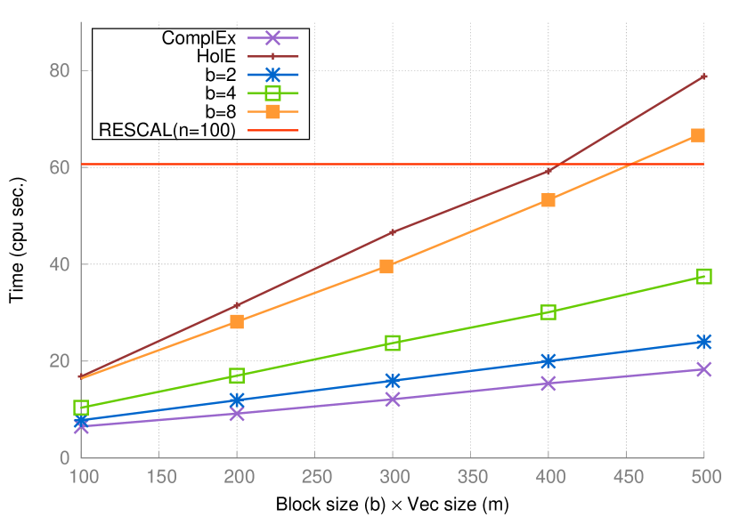
Figure 2: CPU run time per epoch of BlockHolE on WN11 Base with single CPU thread.

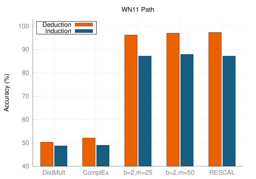
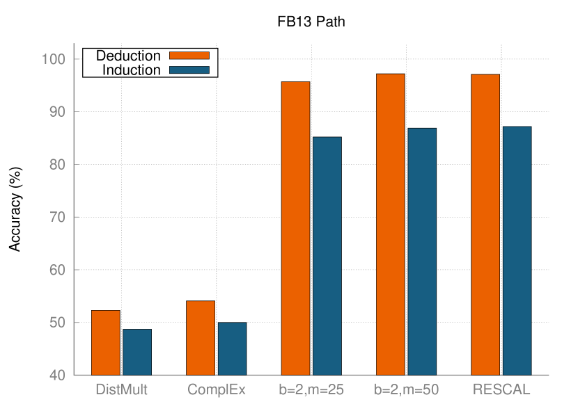
Figure 3: Path QA classification result comparing BlockHolE ($b=2,m=25$ and $b=2,m=50$) to DistMult, ComplEx and RESCAL models (all with $n=50$ as the result of grid search).

The comparison of KGE models was performed in two path QA tasks: (i) ranking and (ii) binary classification tasks.

6.1.1 Path QA ranking

For the path QA ranking task, we adopted the same protocol and dataset used by Guu et al. (2015). Table 2 shows the statistics of their dataset. The dataset consists of two parts, “Base” and “Path”.

The Base part only contains facts (i.e., path queries with $k=1$), and thus it is essentially for evaluating KGC performance. Its training samples constitute the observed facts $\mathcal{F}$, and the facts in the entire Base part (training/validation/test sets) make the ground truth facts $\mathcal{F}^{*}$.

The Path part contains path queries sampled from the same $\mathcal{F}$ and $\mathcal{F}^{*}$ as the Base part. The test samples in the Path part is divided into “deduction” and “induction” sets. In the “deduction” set, test samples were sampled from the Base training graph $\mathcal{G}(\mathcal{F})$. By contrast, in the “induction” set, the test samples were chosen from the ground truth graph $\mathcal{G}(\mathcal{F}^{*})$ such that none of them have a corresponding path in $\mathcal{G}(\mathcal{F})$. Thus, the “induction” set is intended to measure how well a model generalizes to unobserved paths, whereas the “deduction” set is to test its ability to faithfully encode the observed training graph.

At the time of evaluation, for each a test sample $(s,r_{1}/\dots/r_{k},\allowbreak o)$, a candidate set

$$\mathcal{T}(r_{k})=\{t:\exists h\in\mathcal{E}\;(h,r_{k},t)\in\mathcal{F}^{*}\},$$

was first computed. In other words, the candidates are the entities for which $r_{k}$ (i.e., the last relation in the test query) takes as its object at least once in $\mathcal{F}^{*}$. Then, for each compared model, we made the ranking of the candidates entities in $\mathcal{T}(r_{k})$ by the score $\phi(s,r_{1}/\dots/r_{k},\allowbreak e)$, where $\phi$ is learned by the model from the training set.

The quality of the ranking was measured by two evaluation metrics: averaged mean quantile (MQ) and P@10 (percentage of correct answers ranked in the top 10). For $q=s/p$ where $p=r_{1}/\dots/r_{k}$, the correct answer set $\llbracket q\rrbracket$ is the set of all entities that can be reached from $s$ by traversing $p$ over $\mathcal{G}(\mathcal{F}^{*})$. Formally, let $\llbracket s\rrbracket=\{s\}$, and the answer set can be recursively defined: $\llbracket q/r\rrbracket=\{t:\exists h\in\llbracket q\rrbracket,(h,r,t)\in\mathcal{F}^{*}\}$. With these definitions, MQ is computed by the following formula:

$$\frac{|\{o^{\prime}|o^{\prime}\in\mathcal{N}(q):\phi(s,p,o^{\prime})\leq\phi(s,p,o)\}|}{|\mathcal{N}(q)|},$$ (13)

where $\mathcal{N}(q)=\mathcal{T}(r_{k})\setminus\llbracket q\rrbracket$ is the set of incorrect answers. Eq. (13) cannot be computed for queries with which $\mathcal{T}(r_{k})=\llbracket q\rrbracket$, and these queries were excluded from evaluation. For further details, see the original paper by Guu et al. (2015).

6.1.2 Path QA classification

In the path QA classification task, we simply report classification accuracy. After the scoring function $\phi$ was trained with logistic regression, a path query $q=(s,r_{1}/\dots/r_{k},o)$ was classified as true if $\phi(q)\geq 0$, or false otherwise.

Since the test and validation sets of Path in Table 2 contain only correct queries, we sampled negative ones by the following procedure: For a correct query $q=(s,r_{1}/\dots/r_{k},o)$ ($k\geq 2$), we generated its reverse relation path query $q^{\prime}=(s,r_{k}/r_{k-1}/\dots/r_{1},o)$. If $q^{\prime}$ does not exist in $\mathcal{G}(\mathcal{F}^{*})$, we used it as a negative.

6.2 Experiment setup

We compared BlockHolE with state-of-the-art bilinear KGE models: DistMult, RESCAL and ComplEx. We have implemented BlockHolE in Java. BlockHolE reduces to ComplEx when $b=1$, and with the imaginary parts of parameters set to $0$, it reduces to RESCAL when $m=1$ and to DistMult when $b=1$. For a fair run time comparison, however, we separately implemented RESCAL using jblas-1.2.4 for matrix computation. Through all experiments, we optimized the logistic loss with L2 regularization on the parameters $\Theta$:

$$\min_{\Theta}\sum_{(q,y)\in\mathcal{D}}\log\{1+\exp(-y\phi(q;\Theta))\}+\lambda||\Theta||_{2}^{2}$$

where $y$ denotes the truth value of a query $q$ in a training data $\mathcal{D}$. Given a correct query $q=(s,r_{1}/\dots/r_{k},o)$, we generated negative samples by replacing $o$ with an entity randomly sampled from $\mathcal{E}$.

We selected the hyperparameters via grid search such that on the validation set they maximize classification accuracy in the path QA classification task and MQ in the path QA ranking task. For all models except BlockHolE, all combinations of $\lambda\in\allowbreak\{0.0001,\allowbreak 0\}$, learning rate $\eta\in\allowbreak\{0.005,\allowbreak 0.01,\allowbreak 0.025,\allowbreak 0.05\}$, and the embedding size $n\in\{50,100,150,200\}$ were tried during grid search. For BlockHolE, all combinations of $(b,m)\in\allowbreak\{(2,25),\allowbreak(2,50),\allowbreak(2,100),\allowbreak(4,25),\allowbreak(4,50),\allowbreak(8,25)\}$, $\lambda\in\allowbreak\{0.0001,\allowbreak 0\}$ and $\eta\in\allowbreak\{0.005,\allowbreak 0.01,\allowbreak 0.025,\allowbreak 0.05\}$ were tried. The maximum number of training epochs was set to 500. The number of negatives generated per positive sample was 5 during training.

6.3 Results

6.3.1 Path QA ranking

Table 3 shows the results on the path QA ranking data. BlockHolE outperforms other bilinear KGE models considerably both on deductive and inductive test settings. These results strongly suggest that BlockHolE is more expressive in modeling path QA than DistMult and ComplEx, while effectively reducing redundant parameters in RESCAL which can cause model overfitting. Figure 2 shows the empirical scalability of BlockHolE. When $b$ is small, BlockHolE scales linearly in the dimension $n=bm$ of the embedding space.

6.3.2 Path QA classification

Figure 3 shows the accuracy of path QA classification. DistMult and ComplEx were considerably worse than BlockHolE and RESCAL for both WN11 and FB13. This result confirms our claim: The non-commutativity of relation matrices plays a critical role in modeling path QA. The performance of BlockHolE ($b=2,m=25$) was comparable to that of RESCAL but the former was 12 times faster.

6.4 Analysis

Label	Relation Path	ComplEx	BlockHolE
+	*/parents/religion/*	96.7	100.0
-	*/religion/parents/*	3.3	100.0

Table 4: Classification accuracy on selected queries.

The accuracies of BlockHolE and RESCAL on the path QA classification task were markedly better than those of DistMult and ComplEx. We analyzed the results further. We extracted all queries from $\mathcal{G}(\mathcal{F}^{*})$ of FB13 that consist of an interpretable relation path */parents/religion/* where $*$ denotes “can match any relation path”. For such queries $(s,*/\text{parents}/\text{religion}/*,o)$, we also generated meaningless queries $(s,*/\text{religion}/\text{parents}/*,o)$ as negatives. Table 4 shows the classification accuracies of ComplEx and BlockHolE ($b=2,m=25$). The results clearly show that ComplEx cannot correctly answer the negative queries at all due to the lack of the non-commutative property.

7 Summary

In this paper, we have pointed out the problems of existing bilinear KGE models in path QA, and proposed a new model that overcomes these problems. This model, called BlockHolE, represents relations as block circulant matrices. As a result, it respects the order of relations in path queries, while enjoying linear-time computation of scoring functions when the number $b^{2}$ of blocks is sufficiently small. It generalizes HolE/ComplEx, and it can also be interpreted as an interpolation between RESCAL and HolE/ComplEx. Its effectiveness was shown empirically in path QA.

Our proposal can be useful in not only path QA but also many tasks such as associative rule mining Yang et al. (2015), path regularization Lin et al. (2015), and more complex QA Hamilton et al. (2018), in which composite relations need to be embedded as a vector. Other future directions include reducing the increased parameters in the proposed block circulant matrices, such as by using multiplicative L1 regularization for ComplEx Manabe et al. (2018).

Acknowledgments

We thank anonymous reviewers for helpful comments. This work was partially supported by JSPS Kakenhi Grant Numbers 19H04173, 18K11457, and 18H03288.

References

- Bordes et al. (2013) Antoine Bordes, Nicolas Usunier, Alberto Garcia-Duran, Jason Weston, and Oksana Yakhnenko. 2013. Translating embeddings for modeling multi-relational data. In Advances in Neural Information Processing Systems 26 (NIPS), pages 2787–2795.
- Guu et al. (2015) Kelvin Guu, John Miller, and Percy Liang. 2015. Traversing knowledge graphs in vector space. In Proceedings of the 2015 Conference on Empirical Methods in Natural Language Processing (EMNLP), pages 318–327.
- Hamilton et al. (2018) William L. Hamilton, Payal Bajaj, Marinka Zitnik, Dan Jurafsky, and Jure Leskovec. 2018. Embedding logical queries on knowledge graphs. In Advances in Neural Information Processing Systems 31 (NeurIPS), pages 2030–2041.
- Hayashi and Shimbo (2017) Katsuhiko Hayashi and Masashi Shimbo. 2017. On the equivalence of holographic and complex embeddings for link prediction. In Proceedings of the 55th Annual Meeting of the Association for Computational Linguistics (ACL), volume 2: Short Papers, pages 554–559.
- Kazemi and Poole (2018) Seyed Mehran Kazemi and David Poole. 2018. SimplE embedding for link prediction in knowledge graphs. In Advances in Neural Information Processing Systems 31 (NeurIPS), pages 4284–4295.
- Lin et al. (2015) Yankai Lin, Zhiyuan Liu, Huan-Bo Luan, Maosong Sun, Siwei Rao, and Song Liu. 2015. Modeling relation paths for representation learning of knowledge bases. In Proceedings of the 2015 Conference on Empirical Methods in Natural Language Processing (EMNLP), pages 705–714.
- Liu et al. (2017) Hanxiao Liu, Yuexin Wu, and Yiming Yang. 2017. Analogical inference for multi-relational embeddings. In Proceedings of the 34th International Conference on Machine Learning (ICML), pages 2168–2178.
- Manabe et al. (2018) Hitoshi Manabe, Katsuhiko Hayashi, and Masashi Shimbo. 2018. Data-dependent learning of symmetric/anti-symmetric relations for knowledge base completion. In Proceedings of the 32nd AAAI Conference on Artificial Intelligence (AAAI), pages 3754–3761.
- Nickel et al. (2016a) Maximilian Nickel, Kevin Murphy, Volker Tresp, and Evgeniy Gabrilovich. 2016a. A review of relational machine learning for knowledge graphs. Proceedings of the IEEE, 104(1):11–33.
- Nickel et al. (2016b) Maximilian Nickel, Lorenzo Rosasco, and Tomaso Poggio. 2016b. Holographic embeddings of knowledge graphs. In Proceedings of the 30th AAAI Conference on Artificial Intelligence (AAAI), pages 1955–1961.
- Nickel et al. (2011) Maximilian Nickel, Volker Tresp, and Hans-Peter Kriegel. 2011. A three-way model for collective learning on multi-relational data. In Proceedings of the 28th International Conference on Machine Learning (ICML), pages 809–816.
- Trouillon et al. (2016) Théo Trouillon, Johannes Welbl, Sebastian Riedel, Éric Gaussier, and Guillaume Bouchard. 2016. Complex embeddings for simple link prediction. In Proceedings of the 33rd International Conference on Machine Learning (ICML), pages 2071–2080.
- Yang et al. (2015) Bishan Yang, Wen-tau Yih, Xiaodong He, Jianfeng Gao, and Li Deng. 2015. Embedding entities and relations for learning and inference in knowledge bases. In Proceedings of the 3rd International Conference on Learning Representations (ICLR).