Classes of graphs with low complexity:
the case of classes with bounded linear rankwidth

Abstract

Classes with bounded rankwidth are MSO-transductions of trees and classes with bounded linear rankwidth are MSO-transductions of paths – a result that shows a strong link between the properties of these graph classes considered from the point of view of structural graph theory and from the point of view of finite model theory. We take both views on classes with bounded linear rankwidth and prove structural and model theoretic properties of these classes. The structural results we obtain are the following. 1) The number of unlabeled graphs of order $n$ with linear rank-width at most $r$ is at most $\bigl{[}(r/2)!\,2^{\binom{r}{2}}3^{r+2}\bigr{]}^{n}$. 2) Graphs with linear rankwidth at most $r$ are linearly $\chi$-bounded. Actually, they have bounded $c$-chromatic number, meaning that they can be colored with $f(r)$ colors, each color inducing a cograph. 3) To the contrary, based on a Ramsey-like argument, we prove for every proper hereditary family $\mathscr{F}$ of graphs (like cographs) that there is a class with bounded rankwidth that does not have the property that graphs in it can be colored by a bounded number of colors, each inducing a subgraph in $\mathscr{F}$.

From the model theoretical side we obtain the following results: 1) A direct short proof that graphs with linear rankwidth at most $r$ are first-order transductions of linear orders. This result could also be derived from Colcombet’s theorem on first-order transduction of linear orders and the equivalence of linear rankwidth with linear cliquewidth. 2) For a class $\mathscr{C}$ with bounded linear rankwidth the following conditions are equivalent: a) $\mathscr{C}$ is stable, b) $\mathscr{C}$ excludes some half-graph as a semi-induced subgraph, c) $\mathscr{C}$ is a first-order transduction of a class with bounded pathwidth. These results open the perspective to study classes admitting low linear rankwidth covers.

On devient jeune à soixante ans.
Malheureusement, c’est trop tard.
 
You become young when you’re sixty.
Unfortunately, it’s too late.
 
到60岁，我们才开始变得年轻。
不幸的是，为时晚矣。

Pablo Picasso

1 Introduction

A primary concern in many areas of mathematics is to classify structures (or classes of structures) according to their intrinsic complexity. In this paper we consider three approaches and their interplay to the notion of structural complexity: the model theoretic approach based on the standard dividing lines that are stability and dependence, the algebraic approach founding the notion of rankwidth and linear rankwidth, and a more classical graph theoretical approach based on colorings and decompositions of graphs.

A theory of sparse structures was initiated in [33], which mainly fits to the classification of monotone classes. The theory has led to the nowhere dense/somewhere dense dichotomy that can be observed in several areas of graph theory, theoretical computer science, model theory, analysis, category theory and probability theory. Motivated by the connection with model theory – nowhere dense classes are monadically stable [1] and even have low VC-density [37] – and by a possible extension of first-order model-checking algorithms for bounded expansion classes [11, 12] and for nowhere dense classes [17], these notions were extended to classes that are obtained as first-order transductions of sparse classes, the structurally sparse classes [34, 13]. The central tool used in our approach is the transduction machinery, which establishes a fruitful bridge between graph theory and finite model theory. Informally, a first-order transduction is a way to interpret a structure in another structure, where the new structure is defined by means of first-order formulas with set parameters. Indeed, a standard approach of both model theory and computability theory is to determine the relative complexity of two structures by showing that the first interprets in the second, and is therefore not more complex than the second. In this context, important classes of structures are the class of finite linear orders and the class of element to finite set membership graphs (powerset graphs), as they define the two most important model theoretical dividing lines: stability, which corresponds to the impossibility to interpret arbitrarily large linear orders, and dependence (or NIP, for “Non-Independence Property”), which corresponds to the the impossibility to interpret arbitrarily large membership graphs. The versions of these properties where we allow set parameters are monadic stability and monadic dependence.

The use of first-order transductions naturally fits the study of hereditary classes. If we consider classes that are obtained as first-order transductions of other classes, the natural tractability limit is the realm of monadically NIP structures, as non monadically NIP classes allow to interpret the whole class of finite graphs. In this world, typical well behaved monadically NIP but monadically unstable classes of graphs are classes with bounded rankwidth (like cographs) and classes with bounded linear rankwidth (like half-graphs). This justifies a specific study of these classes, as well as the classes that admit finite $p$-covers with bounded rankwidth [26] or classes that admit finite $p$-covers with bounded linear rankwidth (like unit interval graphs), as they naturally extend structurally bounded expansion classes, which admit finite $p$-covers with bounded shrubdepth [13]. However we do not know whether classes with such covers are monadically NIP. The whole framework is schematically pictured on Figure 1.

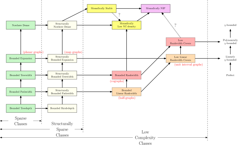
Figure 1: Inclusion map of graph classes. Some examples of classes are given in brackets.

This paper consists of two parts. The first part sets the scene and builds the framework that supports our study. The second part roots our study in concrete problems. In particular, we consider classes with bounded linear rankwidth and show how model theoretic and structural properties of classes with bounded linear rankwidth allow to prove new properties of these classes. In particular we prove the following theorems (formal definitions will be given in Section 2).

Theorem 4.6.

Let $\mathscr{C}$ be a class of graphs with bounded linear rankwidth. Then the following are equivalent:

1. $\mathscr{C}$ is stable,

2. $\mathscr{C}$ is monadically stable,

3. $\mathscr{C}$ has $2$-covers with bounded shrubdepth,

4. $\mathscr{C}$ is sparsifiable,

5. $\mathscr{C}$ excludes some semi-induced half-graph,

6. $\mathscr{C}$ is a first-order transduction of a class with bounded expansion (i.e. has structurally bounded expansion),

7. $\mathscr{C}$ is a first-order transduction of a class with bounded pathwidth (i.e. has structurally bounded pathwidth).

And we deduce

Theorem 6.2.

Let $\mathscr{C}$ be a class with low linear rankwidth covers. Then the following are equivalent:

1. $\mathscr{C}$ is monadically stable,

2. $\mathscr{C}$ is stable,

3. $\mathscr{C}$ excludes a semi-induced half-graph,

4. $\mathscr{C}$ has structurally bounded expansion.

From the graph theoretic point of view, we briefly discuss how classes with bounded rankwidth differ from classes with bounded linear rankwidth and give some lower bounds for $\chi$-boundedness of graphs with bounded rankwidth and for graphs with bounded linear rankwidth. Then we prove upper bounds for graphs with bounded linear rankwidth.

Theorem 5.17.

Every graph $G$ with linear rankwidth at most $r$ can be colored with at most $3(r+2)!2^{\binom{r+1}{2}}$ colors such that each color induces a cograph with cotree height at most $r+2$. In particular, for every graph $G$ with linear rankwidth at most $r$ we have

$$\chi(G)\leq 3(r+2)!2^{\binom{r+1}{2}}\,\omega(G).$$

Theorem 4.6 and a weaker form of Theorem 5.17 (Theorem 4.3) are proved in Section 4 by using the notion of linear NLC-width expression and Simon’s factorization forest theorem.

The strong form of Theorem 5.17 is proved in Section 5 by a fine analysis of linear rankwidth decompositions. Along the way we also obtain an upper bound for the number of graphs with linear rankwidth at most $r$.

Theorem 5.15.

Unlabeled graphs with linear rankwidth at most $r$ can be encoded using at most $\binom{r}{2}+r\log_{2}r+\log_{2}(3/e)r+O(\log_{2}r)$ bits per vertex. Precisely, the number of unlabelled graphs of order $n$ with linear rankwidth at most $r$ is at most $\left[(r+2)!\,2^{\binom{r}{2}}3^{r+2}\right]^{n}$.

2 Classes with low complexity

2.1 Structures and logic

A signature $\Sigma$ is a finite set of relation and function symbols, each with a prescribed arity. In this paper we consider only signatures with relation symbols. A $\Sigma$-structure $\mathbf{A}$ consists of a finite universe (or domain) $V(\mathbf{A})$ and interpretations of the symbols in the signature: each relation symbol $R\in\Sigma$, say of arity $k$, is interpreted as a $k$-ary relation $R^{\mathbf{A}}\subseteq V(\mathbf{A})^{k}$. For a signature $\Sigma$, we consider standard first-order logic over $\Sigma$. If $\mathbf{A}$ is a structure and $X\subseteq V(\mathbf{A})$ then we denote by $\mathbf{A}[X]$ the substructure of $\mathbf{A}$ induced by $X$. The Gaifman graph of a structure $\mathbf{A}$ is the graph with vertex set $V(\mathbf{A})$ where two distinct elements $u,v\in\mathbf{A}$ are adjacent if and only if $u$ and $v$ appear together in some tuple in some relation of $\mathbf{A}$. For a formula $\varphi(x_{1},\dots,x_{k})$ with $k$ free variables and a structure $\mathbf{A}$, we define

$$\varphi(\mathbf{A})=\{(v_{1},\dots,v_{k})\in V(\mathbf{A})^{k}~{}:~{}\mathbf{A}\models\varphi(v_{1},\dots,v_{k})\}.$$

We usually write $\bar{x}$ for a tuple $(x_{1},\dots,x_{k})$ of variables and leave it to the context to determine the length of the tuple. The above equality then rewrites as $\varphi(\mathbf{A})=\{\bar{v}\in V(\mathbf{A})^{|\bar{x}|}~{}:~{}\mathbf{A}\models\varphi(\bar{v})\}$. Also, for a formula $\varphi(\bar{x},\bar{y})$ and $\bar{b}\in V(\mathbf{A})^{|\bar{y}|}$ we define

$$\varphi(\bar{b},\mathbf{A})=\{\bar{v}\in V(\mathbf{A})^{|\bar{x}|}~{}:~{}\mathbf{A}\models\varphi(\bar{v},\bar{b})\}.$$

A monadic lift $\Lambda$ of a $\Sigma$-structure $\mathbf{A}$ is a $\Sigma^{+}$-structure $\Lambda(\mathbf{A})$ such that $\Sigma^{+}$ is the union of $\Sigma$ and a set of unary relation symbols and $\mathbf{A}$ is the shadow of $\Lambda(\mathbf{A})$, that is the $\Sigma$-structure obtained from $\Lambda(\mathbf{A})$ by “forgetting” all the relations in $\Sigma^{+}\setminus\Sigma$.

2.2 Graphs, colored graphs and trees.

Graphs can be viewed as finite structures over the signature consisting of a binary relation symbol $E$, interpreted as the edge relation, in the usual way. For a finite label set $\Gamma$, by a $\Gamma$-colored graph we mean a graph enriched by a unary predicate $U_{\gamma}$ for each $\gamma\in\Gamma$. A rooted forest is an acyclic graph $F$ together with a unary predicate $R\subseteq V(F)$ selecting one root in each connected component of $F$. A tree is a connected forest. The depth of a node $x$ in a rooted forest $F$ is the number of vertices in the unique path between $x$ and the root of the connected component of $x$ in $F$. In particular, $x$ is a root of $F$ if and only if $F$ has depth $1$ in $F$. The depth of a forest is the largest depth of any of its nodes. The least common ancestor of nodes $x$ and $y$ in a rooted tree is the common ancestor of $x$ and $y$ that has the largest depth.

2.3 Sparse graph classes

Treewidth, pathwidth and treedepth.

Treewidth is an important width parameter of graphs that was introduced in [40] as part of the graph minors project. Pathwidth is a more restricted width measure that was introduced in [39]. The notion of treedepth was introduced in [29].

For our purposes it will be convenient to define these width measures in terms of intersection graphs. Let $S_{1},\ldots,S_{n}$ be a family of sets. The intersection graph defined by this family is the graph with vertex set $\{v_{1},\ldots,v_{n}\}$ and edge set $\{\{v_{i},v_{j}\}:S_{i}\cap S_{j}\neq\emptyset\}$.

A chordal graph is the intersection graph of a family of subtrees of a tree. An interval graph is the intersection graph of a family of intervals. A trivially perfect graph is the intersection graph of a family of nested intervals. Alternatively, a trivially perfect graph is the comparability graph of a bounded depth tree order.

The treewidth of a graph $G$ is one less than the minimum clique number of a chordal supergraph of $G$, the pathwidth of a graph $G$ is one less than the minimum clique number of an interval supergraph of $G$, and the treedepth of a graph $G$ is the minimum clique number of a trivially perfect supergraph of $G$:

$$\mathrm{tw}(G) =\min\{\omega(H)-1~{}:~{}H\text{ chordal and }H\supseteq G\},$$

$$\mathrm{pw}(G) =\min\{\omega(H)-1~{}:~{}H\text{ interval graph and }H\supseteq G\},$$

$$\mathrm{td}(G) =\min\{\omega(H)~{}:~{}H\text{ trivially perfect and }H\supseteq G\}.$$

A class $\mathscr{C}$ of graphs has bounded treewidth, bounded pathwidth, or bounded treedepth, respectively, if there is a bound $k\in\mathbb{N}$ such that every graph in $\mathscr{C}$ has treewidth, pathwidth, or treedepth, respectively, at most $k$.

Classes with bounded expansion.

A graph $H$ is a depth-$r$ topological minor of a graph $G$ if $G$ contains a subgraph isomorphic to a $\leq 2r$-subdivision of $H$. A class $\mathscr{C}$ of graphs has bounded expansion if there is a function $f\colon\mathbb{N}\rightarrow\mathbb{N}$ such that $\frac{\|H\|}{|H|}\leq f(r)$ for every $r\in\mathbb{N}$ and every depth-$r$ topological minor $H$ of a graph from $\mathscr{C}$. Examples of classes with bounded expansion include the class of planar graphs, any class of graphs with bounded maximum degree, or more generally, any class of graphs that excludes a fixed topological minor. We lift the notion with bounded expansion to classes of structures over an arbitrary fixed signature, by requiring that their class of Gaifman graphs has bounded expansion. In particular, a class of colored graphs has bounded expansion if and only if the class of underlying uncolored graphs has bounded expansion. For an in-depth study of classes with bounded expansion we refer the reader to the monography [33].

Nowhere dense classes.

A class $\mathscr{C}$ is nowhere dense if there is a function $f\colon\mathbb{N}\rightarrow\mathbb{N}$ such that $\omega(H)\leq f(r)$ for every $r\in\mathbb{N}$ and every depth-$r$ topological minor $H$ of a graph from $\mathscr{C}$ [31, 32].

2.4 Monadic stability, monadic dependence, and low VC-density

The model theoretic approach of complexity is based on the study of properties rather than on the study of objects. This is witnessed by the fact that the central subjects of study in model theory are theories and that the actual structures are only considered as models of theories. Nevertheless, most notions defined on theories have their counterpart on models or on classes of models. One of the main goals of stability theory (also known as classification theory) is to classify the models of a given first-order theory according to some simple system of cardinal invariants. In this respect, elementary theories are stable theories and still reasonably well behaved theories are NIP theories (also called dependent theories). These notions can be translated to classes of structures as follows:

Definition 2.1.

A class $\mathscr{C}$ of structures is stable if for every first-order formula $\varphi(\bar{x},\bar{y})$ there exists an integer $k$ such that for every structure $\mathbf{A}\in\mathscr{C}$ and for all tuples $\bar{a}_{1},\dots,\bar{a}_{\ell},\bar{b}_{1},\dots,\bar{b}_{\ell}$ of elements of $\mathbf{A}$, if

$$\mathbf{A}\models\varphi(\bar{a}_{i},\bar{b}_{j})\quad\iff\quad i<j$$ (1)

for all $i,j\in[\ell]$, then $\ell\leq k$.

Definition 2.2.

A class $\mathscr{C}$ of structures is dependent (or NIP) if for every first-order formula $\varphi(\bar{x},\bar{y})$ there exists an integer $k$ such that for every structure $\mathbf{A}\in\mathscr{C}$ and for all tuples $\bar{a}_{i}$ ($i\in[\ell]$) and, $\bar{b}_{I}$ ($I\subseteq[\ell]$) of elements of $\mathbf{A}$, if

$$\mathbf{A}\models\varphi(\bar{a}_{i},\bar{b}_{I})\quad\iff\quad i\in I$$ (2)

for all $i\in[\ell]$ and all $I\subseteq[\ell]$, then $\ell\leq k$.

A stronger notion of stability and of dependence arises when one allows to apply arbitrary monadic lifts to the structures in $\mathscr{C}$ before using the formula $\varphi$. These variants are called monadic stability and monadic dependence. The expressive power gained by the monadic lift is so strong that tuples of free variables can be replaced by single free variables in the above definitions [3].

Definition 2.3.

A class $\mathscr{C}$ of structures is monadically stable if for every first-order formula $\varphi(x,y)$ there exists an integer $k$ such that for every monadic lift $\mathbf{A}^{+}$ of a structure $\mathbf{A}\in\mathscr{C}$ and for all elements $a_{1},\dots,a_{\ell},b_{1},\dots,b_{\ell}$ of $\mathbf{A}$, if

$$\mathbf{A}^{+}\models\varphi(a_{i},b_{j})\quad\iff\quad i<j$$ (3)

for all $i,j\in[\ell]$, then $\ell\leq k$.

Definition 2.4.

A class $\mathscr{C}$ of structures is monadically dependent (or monadically NIP) if for every first-order formula $\varphi(x,y)$ there exists an integer $k$ such that for every monadic lift $\mathbf{A}^{+}$ of a structure $\mathbf{A}\in\mathscr{C}$ and for all elements $a_{i}$ ($i\in[\ell]$) and $b_{I}$ ($I\subseteq[\ell]$) of $\mathbf{A}$, if

$$\mathbf{A}^{+}\models\varphi(a_{i},b_{I})\quad\iff\quad i\in I$$ (4)

for all $i\in[\ell]$ and all $I\subseteq[\ell]$, then $\ell\leq k$.

For a formula $\varphi(\bar{x},\bar{y})$, the VC-density $\mathrm{vc}^{\mathscr{C}}(\varphi)$ of a formula $\varphi$ in a class $\mathscr{C}$ (containing arbitrarily large structures) is defined as

$$\mathrm{vc}^{\mathscr{C}}(\varphi)=\lim_{t\rightarrow\infty}\sup_{\mathbf{A}\in\mathscr{C}}\sup_{\begin{subarray}{c}B\subseteq V(\mathbf{A})\\ |B|=t\end{subarray}}\frac{\log|\{\varphi(\bar{v},\mathbf{A})\cap B^{|\bar{x}|}~{}:~{}\bar{v}\in V(\mathbf{A})^{|\bar{y}|}\}|}{\log|B|}$$

The VC-density $\mathrm{vc}^{\mathscr{C}}$ of the class $\mathscr{C}$ is

$$\mathrm{vc}^{\mathscr{C}}(n)=\sup\{\mathrm{vc}^{\mathscr{C}}(\varphi)~{}:~{}\varphi(\bar{x};\bar{y})\text{ is a formula with }|\bar{y}|=n\}.$$

According to the Sauer-Shelah Lemma [41, 42], a class $\mathscr{C}$ is NIP if and only if $\mathrm{vc}^{\mathscr{C}}(\varphi)<\infty$ for every formula $\varphi$. However, it is possible for a NIP class (and even for a stable class) to have $\mathrm{vc}^{\mathscr{C}}(1)=\infty$. On the other hand, is easily checked that (unless structures in $\mathscr{C}$ have bounded size) for every positive integer $n$ we have $\mathrm{vc}^{\mathscr{C}}(n)\geq n$. A class $\mathscr{C}$ has low VC-density if $\mathrm{vc}^{\mathscr{C}}(n)=n$ for all integers $n$ [18]. We say that $\mathscr{C}$ has monadically low VC-density if every monadic lift of $\mathscr{C}$ has low VC-density.

Theorem 2.5.

Let $\mathscr{C}$ be a class of graphs.

1. If $\mathscr{C}$ is nowhere dense, then $\mathscr{C}$ is monadically stable ([Adler, Adler [1]; Podewski, Ziegler [38]).

2. If $\mathscr{C}$ is nowhere dense, then $\mathscr{C}$ has monadicallly low VC-density (Pilipczuk, Siebertz, and Toruńczyk [37]]).

Theorem 2.6 ([Adler, Adler [1]; Podewski, Ziegler [38]).

Let $\mathscr{C}$ be a monotone class of graphs. If $\mathscr{C}$ is NIP, then $\mathscr{C}$ is nowhere dense.

Corollary 2.1.

Let $\mathscr{C}$ be a monotone class of graphs. Then the following are equivalent.

1. $\mathscr{C}$ is nowhere dense,

2. $\mathscr{C}$ is stable,

3. $\mathscr{C}$ is monadically stable,

4. $\mathscr{C}$ is NIP,

5. $\mathscr{C}$ is monadically NIP,

6. $\mathscr{C}$ has low VC-density,

7. $\mathscr{C}$ has monadically low VC-density.

2.5 Interpretations and transductions

In this paper, by an interpretation of $\Sigma^{\prime}$-structures in $\Sigma$-structures we mean a transformation $\mathsf{I}$ defined by means of formulas $\varphi_{R}(\bar{x})$ (for $R\in\Sigma^{\prime}$ of arity $|\bar{x}|$) and a formula $\nu(x)$. For every $\Sigma$-structure $\mathbf{A}$, the $\Sigma^{\prime}$-structure $\mathsf{I}(\mathbf{A})$ has domain $\nu(\mathbf{A})$ and the interpretation of each relation $R\in\Sigma^{\prime}$ is given by $R^{\mathsf{I}(\mathbf{A})}=\varphi_{R}(\mathbf{A})\cap\nu(\mathbf{A})^{|\bar{x}|}$.

A transduction $\mathsf{T}$ is the composition $\mathsf{I}\circ\Lambda$ of a monadic lift and an interpretation. It is easily checked that the composition of two transductions is again a transduction.

Let $\mathscr{C}$ and $\mathscr{D}$ be classes of $\Sigma_{\mathscr{C}}$-structures and $\Sigma_{\mathscr{D}}$-structures, respectively. Let $\mathsf{I}$ be an interpretation of $\Sigma_{\mathscr{D}}$-structures in $\Sigma_{\mathscr{C}}^{+}$-structures, where $\Sigma_{\mathscr{C}}^{+}\setminus\Sigma_{\mathscr{C}}$ is a finite set of unary relation symbols. If, for every $\mathbf{B}$ in $\mathscr{D}$ there exists a lift $\mathbf{A}^{+}$ of some structure $\mathbf{A}\in\mathscr{C}$ such that $\mathbf{B}=\mathsf{I}(\mathbf{A}^{+})$ we write

and we write

if there exists $\mathsf{I}$ such that Let $\mathscr{H}$ denote the class of half graphs and let $\mathscr{G}$ denote the class of all finite graphs. We have

$$\mathscr{C}\text{ is monadically stable}\quad \iff\quad\lx@xy@svg{\hbox{\raise 0.0pt\hbox{\kern 6.61111pt\hbox{\ignorespaces\ignorespaces\ignorespaces\hbox{\vtop{\kern 0.0pt\offinterlineskip\halign{\entry@#!@&&\entry@@#!@\cr&\\}}}\ignorespaces{\hbox{\kern-6.61111pt\raise 0.0pt\hbox{\hbox{\kern 0.0pt\raise 0.0pt\hbox{\hbox{\kern 3.0pt\raise 0.0pt\hbox{$\textstyle{\mathscr{C}\ignorespaces\ignorespaces\ignorespaces\ignorespaces\ignorespaces}$}}}}}}}\ignorespaces\ignorespaces\ignorespaces\ignorespaces{}{\hbox{\lx@xy@droprule}}\ignorespaces{\hbox{\kern 14.46097pt\raise 0.0pt\hbox{\hbox{\kern 0.0pt\raise-1.75pt\hbox{$\scriptstyle{/}$}}}}}{\hbox{\lx@xy@droprule}}\ignorespaces{\hbox{\kern 30.61111pt\raise 0.0pt\hbox{\hbox{\kern 0.0pt\raise 0.0pt\hbox{\hbox{\kern-3.0pt\lower 0.0pt\hbox{\lx@xy@tip{1}\lx@xy@tip{-1}}}\lx@xy@tip{1}\lx@xy@tip{-1}}}}}}{\hbox{\lx@xy@droprule}}{\hbox{\lx@xy@droprule}}{\hbox{\kern 30.61111pt\raise 0.0pt\hbox{\hbox{\kern 0.0pt\raise 0.0pt\hbox{\hbox{\kern 3.0pt\raise 0.0pt\hbox{$\textstyle{\mathscr{H}.}$}}}}}}}\ignorespaces}}}}\ignorespaces \textstyle{\mathscr{C}\ignorespaces\ignorespaces\ignorespaces\ignorespaces\ignorespaces} \scriptstyle{/} \textstyle{\mathscr{H}.} \textstyle{\mathscr{C}\ignorespaces\ignorespaces\ignorespaces\ignorespaces\ignorespaces} \scriptstyle{/} \textstyle{\mathscr{H}.}$$

$$\mathscr{C}\text{ is monadically NIP}\quad \iff\quad\lx@xy@svg{\hbox{\raise 0.0pt\hbox{\kern 6.61111pt\hbox{\ignorespaces\ignorespaces\ignorespaces\hbox{\vtop{\kern 0.0pt\offinterlineskip\halign{\entry@#!@&&\entry@@#!@\cr&\\}}}\ignorespaces{\hbox{\kern-6.61111pt\raise 0.0pt\hbox{\hbox{\kern 0.0pt\raise 0.0pt\hbox{\hbox{\kern 3.0pt\raise 0.0pt\hbox{$\textstyle{\mathscr{C}\ignorespaces\ignorespaces\ignorespaces\ignorespaces\ignorespaces}$}}}}}}}\ignorespaces\ignorespaces\ignorespaces\ignorespaces{}{\hbox{\lx@xy@droprule}}\ignorespaces{\hbox{\kern 14.46097pt\raise 0.0pt\hbox{\hbox{\kern 0.0pt\raise-1.75pt\hbox{$\scriptstyle{/}$}}}}}{\hbox{\lx@xy@droprule}}\ignorespaces{\hbox{\kern 30.61111pt\raise 0.0pt\hbox{\hbox{\kern 0.0pt\raise 0.0pt\hbox{\hbox{\kern-3.0pt\lower 0.0pt\hbox{\lx@xy@tip{1}\lx@xy@tip{-1}}}\lx@xy@tip{1}\lx@xy@tip{-1}}}}}}{\hbox{\lx@xy@droprule}}{\hbox{\lx@xy@droprule}}{\hbox{\kern 30.61111pt\raise 0.0pt\hbox{\hbox{\kern 0.0pt\raise 0.0pt\hbox{\hbox{\kern 3.0pt\raise 0.0pt\hbox{$\textstyle{\mathscr{G}.}$}}}}}}}\ignorespaces}}}}\ignorespaces \textstyle{\mathscr{C}\ignorespaces\ignorespaces\ignorespaces\ignorespaces\ignorespaces} \scriptstyle{/} \textstyle{\mathscr{G}.} \textstyle{\mathscr{C}\ignorespaces\ignorespaces\ignorespaces\ignorespaces\ignorespaces} \scriptstyle{/} \textstyle{\mathscr{G}.}$$

Lemma 2.7 ([2]).

A stable class $\mathscr{C}$ is monadically unstable if and only $\mathscr{C}$ has a transduction to the class of all $1$-subdivided complete bipartite graphs.

Corollary 2.2.

A class $\mathscr{C}$ is monadically stable if and only if it is both stable and monadically NIP.

Figure 2: The half-graph $H_{k}$

We use the term of structurally xxx for classes that are transductions of classes that are xxx. For instance, a class has structurally bounded treewidth if it is the transduction of a class with bounded treewidth.

The following characterizations of classes with bounded treewidth, pathwidth, rankwidth, linear rankwidth, and shrubdepth show the deep connections between these width measures and logical transductions (and at this point will serve as a definition of the notions of rankwidth, linear rankwidth and shrubdepth).

1. A class $\mathscr{C}$ of graphs has bounded treewidth (pathwidth, respectively) if and only if there exists an MSO-transduction $\mathsf{T}$ such that the incidence graph of every $G\in\mathscr{C}$ is the result of applying $\mathsf{T}$ to some tree (path, respectively) ([6] (see also [7], Theorem 7.47)).

2. A class $\mathscr{C}$ of graphs has bounded rankwidth (linear rankwidth, respectively) if and only if there exists an MSO-transduction $\mathsf{T}$ such that every $G\in\mathscr{C}$ is the result of applying $\mathsf{T}$ to some tree (path, respectively). ([6] (see also [7], Theorem 7.47)).

3. A class $\mathscr{C}$ of graphs has bounded rankwidth (linear rankwidth, respectively) if and only if there exists an FO-transduction $\mathsf{T}$ such that every $G\in\mathscr{C}$ is the result of applying $\mathsf{T}$ to some tree order (linear order, respectively) ([5]).

4. A class $\mathscr{C}$ of graphs has bounded shrubdepth if and only if there exists an FO-transduction $\mathsf{T}$ and a height $h$ such that every $G\in\mathscr{C}$ is the result of applying $\mathsf{T}$ to some tree of depth at most $h$ ([15, 14]).

We can rewrite properties (3) and (4) as follows:

$$\mathscr{C}\text{ has bounded rankwidth}\quad \iff\quad\lx@xy@svg{\hbox{\raise 0.0pt\hbox{\kern 8.92778pt\hbox{\ignorespaces\ignorespaces\ignorespaces\hbox{\vtop{\kern 0.0pt\offinterlineskip\halign{\entry@#!@&&\entry@@#!@\cr&\\}}}\ignorespaces{\hbox{\kern-8.92778pt\raise 0.0pt\hbox{\hbox{\kern 0.0pt\raise 0.0pt\hbox{\hbox{\kern 3.0pt\raise 0.0pt\hbox{$\textstyle{\mathscr{Y}^{\leq}\ignorespaces\ignorespaces\ignorespaces\ignorespaces}$}}}}}}}\ignorespaces\ignorespaces\ignorespaces\ignorespaces{}{\hbox{\lx@xy@droprule}}\ignorespaces{\hbox{\kern 32.92778pt\raise 0.0pt\hbox{\hbox{\kern 0.0pt\raise 0.0pt\hbox{\hbox{\kern-3.0pt\lower 0.0pt\hbox{\lx@xy@tip{1}\lx@xy@tip{-1}}}\lx@xy@tip{1}\lx@xy@tip{-1}}}}}}{\hbox{\lx@xy@droprule}}{\hbox{\lx@xy@droprule}}{\hbox{\kern 32.92778pt\raise 0.0pt\hbox{\hbox{\kern 0.0pt\raise 0.0pt\hbox{\hbox{\kern 3.0pt\raise 0.0pt\hbox{$\textstyle{\mathscr{C},}$}}}}}}}\ignorespaces}}}}\ignorespaces \textstyle{\mathscr{Y}^{\leq}\ignorespaces\ignorespaces\ignorespaces\ignorespaces} \textstyle{\mathscr{C},} \textstyle{\mathscr{Y}^{\leq}\ignorespaces\ignorespaces\ignorespaces\ignorespaces} \textstyle{\mathscr{C},}$$

$$\mathscr{C}\text{ has bounded linear rankwidth}\quad \iff\quad\lx@xy@svg{\hbox{\raise 0.0pt\hbox{\kern 8.30278pt\hbox{\ignorespaces\ignorespaces\ignorespaces\hbox{\vtop{\kern 0.0pt\offinterlineskip\halign{\entry@#!@&&\entry@@#!@\cr&\\}}}\ignorespaces{\hbox{\kern-8.30278pt\raise 0.0pt\hbox{\hbox{\kern 0.0pt\raise 0.0pt\hbox{\hbox{\kern 3.0pt\raise 0.0pt\hbox{$\textstyle{\mathscr{L}^{\leq}\ignorespaces\ignorespaces\ignorespaces\ignorespaces}$}}}}}}}\ignorespaces\ignorespaces\ignorespaces\ignorespaces{}{\hbox{\lx@xy@droprule}}\ignorespaces{\hbox{\kern 32.30278pt\raise 0.0pt\hbox{\hbox{\kern 0.0pt\raise 0.0pt\hbox{\hbox{\kern-3.0pt\lower 0.0pt\hbox{\lx@xy@tip{1}\lx@xy@tip{-1}}}\lx@xy@tip{1}\lx@xy@tip{-1}}}}}}{\hbox{\lx@xy@droprule}}{\hbox{\lx@xy@droprule}}{\hbox{\kern 32.30278pt\raise 0.0pt\hbox{\hbox{\kern 0.0pt\raise 0.0pt\hbox{\hbox{\kern 3.0pt\raise 0.0pt\hbox{$\textstyle{\mathscr{C},}$}}}}}}}\ignorespaces}}}}\ignorespaces \textstyle{\mathscr{L}^{\leq}\ignorespaces\ignorespaces\ignorespaces\ignorespaces} \textstyle{\mathscr{C},} \textstyle{\mathscr{L}^{\leq}\ignorespaces\ignorespaces\ignorespaces\ignorespaces} \textstyle{\mathscr{C},}$$

$$\mathscr{C}\text{ has bounded shrubdepth}\quad \iff\quad\exists n\ \lx@xy@svg{\hbox{\raise 0.0pt\hbox{\kern 8.43066pt\hbox{\ignorespaces\ignorespaces\ignorespaces\hbox{\vtop{\kern 0.0pt\offinterlineskip\halign{\entry@#!@&&\entry@@#!@\cr&\\}}}\ignorespaces{\hbox{\kern-8.43066pt\raise 0.0pt\hbox{\hbox{\kern 0.0pt\raise 0.0pt\hbox{\hbox{\kern 3.0pt\raise 0.0pt\hbox{$\textstyle{\mathscr{Y}_{n}\ignorespaces\ignorespaces\ignorespaces\ignorespaces}$}}}}}}}\ignorespaces\ignorespaces\ignorespaces\ignorespaces{}{\hbox{\lx@xy@droprule}}\ignorespaces{\hbox{\kern 32.43066pt\raise 0.0pt\hbox{\hbox{\kern 0.0pt\raise 0.0pt\hbox{\hbox{\kern-3.0pt\lower 0.0pt\hbox{\lx@xy@tip{1}\lx@xy@tip{-1}}}\lx@xy@tip{1}\lx@xy@tip{-1}}}}}}{\hbox{\lx@xy@droprule}}{\hbox{\lx@xy@droprule}}{\hbox{\kern 32.43066pt\raise 0.0pt\hbox{\hbox{\kern 0.0pt\raise 0.0pt\hbox{\hbox{\kern 3.0pt\raise 0.0pt\hbox{$\textstyle{\mathscr{C},}$}}}}}}}\ignorespaces}}}}\ignorespaces \textstyle{\mathscr{Y}_{n}\ignorespaces\ignorespaces\ignorespaces\ignorespaces} \textstyle{\mathscr{C},} \textstyle{\mathscr{Y}_{n}\ignorespaces\ignorespaces\ignorespaces\ignorespaces} \textstyle{\mathscr{C},}$$

where $\mathscr{Y}^{\leq}$ denotes the class of all finite tree orders, $\mathscr{L}^{\leq}$ denotes the class of all linear orders, and $\mathscr{Y}_{n}$ denotes the class of trees with depth at most $n$.

Note that in the characterizations above $\mathscr{Y}^{\leq}$ can be replaced by the class of trivially perfect graphs (or by the larger class of cographs) and $\mathscr{L}^{\leq}$ can be replaced by the class of transitive tournaments or by the class of half-graphs.

Remark 2.8.

Since the class of all graphs does not have bounded rankwidth, we deduce that if $\mathscr{C}$ has bounded rankwidth we have Hence every class with bounded rankwidth is monadically NIP.

In particular, Corollary 2.2 implies the following:

Remark 2.9.

A class with bounded rankwidth is monadically stable if and only if it is stable.

2.6 Weakly sparse classes

It appears that a basic property that makes a graph class dense is that graphs in it contain arbitrarily large bicliques. Indeed, forbidding a biclique as a subgraph (or, equivalently, forbidding a clique and a biclique as induced subgraphs) is known to have a strong consequence on classes with low complexity. We call a class $\mathscr{C}$ weakly sparse if it excludes some biclique as a subgraph.

Theorem 2.10.

Let $\mathscr{C}$ be a weakly sparse class of graphs.

1. If $\mathscr{C}$ has bounded shrubdepth, then $\mathscr{C}$ has bounded treedepth [13].

2. If $\mathscr{C}$ has bounded linear rankwidth, then $\mathscr{C}$ has bounded pathwidth [20].

3. If $\mathscr{C}$ has bounded rankwidth, then $\mathscr{C}$ has bounded treewidth [20].

We call a class sparsifiable if it is transduction-equivalent to a weakly sparse class.

Importance of weakly sparse classes are witnessed by numerous result. Among them, let us cite

• The $k$-Dominating Set problem is fixed parameter tractable (FPT) and has a polynomial kernel for any weakly sparse class [36].

• Connected $k$-Dominating Set, Independent $k$-Dominating Set and Minimum Weight $k$-Dominating Set are FPT, when parameterized by $t+k$ (where $t$ is the output size) [44].

• Dominating Set Reconfiguration is FPT on weakly sparse classes [27].

• For every graph $H$ and for weakly sparse class $\mathscr{C}$ there exists $d\in\mathbb{N}$ such that every graph $G\in\mathscr{C}$ with average degree at least $d$ contains an induced subdivision of $H$ [25]. This result has further been strengthened as follows: every weakly sparse class that excludes an induced subdivision of some graph $H$ has bounded expansion [10].

The assumption that a class is weakly sparse allows frequently to work with induced subgraph instead of subgraphs. For instance:

Theorem 2.11 (Dvořák [10]).

A hereditary weakly sparse class $\mathscr{C}$ has bounded expansion if and only if there exists a function $f\colon\mathbb{N}\rightarrow\mathbb{N}$ such that for every graph $H$, if the $\leq k$-subdivision of $H$ belongs to $\mathscr{C}$ then the average degree of $H$ is at most $f(k)$.

We now prove a similar characterization of nowhere dense classes.

Theorem 2.12.

A hereditary weakly sparse class $\mathscr{C}$ is nowhere dense if and only if there exists a function $f\colon\mathbb{N}\rightarrow\mathbb{N}$ such that the class $\mathscr{C}$ contains no $\leq k$-subdivided clique of order greater than $f(k)$.

This theorem directly follows from the next lemma.

Lemma 2.13.

For all integers $t,p,n$ there exists an integer $N$ such that if a graph $G$ contains no $K_{t,t}$ as a subgraph and no induced $q$-subdivision of $K_{4t}$ (for any $q\leq p$), then it contains no $\leq p$-subdivision of $K_{N}$ as a subgraph.

Proof.

Assume that $G$ contains no $K_{t,t}$ as a subgraph but contains a $\leq p$-subdivision of a large complete graph $K_{N}$ as a subgraph. We can first assume by Ramsey’s theorem that $G$ contains an exact $q$-subdivision of $K_{N}$ (for some $q\leq p$). Of course $q>1$, for otherwise the “subdivision” is induced. Also we can assume that each branch of the subdivision is an induced path (for otherwise we consider a shorter path).

Let $v_{1},\dots,v_{N}$ be the principal vertices of the $K_{N}$, and let $u_{i,j,k}$ (for $1\leq i<j\leq N$ and $1\leq k\leq q$) be the $k$th vertex on the path of length $q+1$ linking $v_{i}$ to $v_{j}$ in the considered $q$-subdivision of $K_{N}$. To every $3$-tuple $(a,b,c)$ (resp. every $4$-tuple $(a,b,c,d)$) of distinct integers in $[N]$ (with $a<b<c$, resp. $a<b<c<d$) we associate its type, which is the isomorphism type of the (vertex ordered) graph induced by $v_{a},v_{b},v_{c}$ (resp. $v_{a},v_{b},v_{c},v_{d}$) and the paths of length $q+1$ linking these vertices. By Ramsey’s theorem, assuming $N$ is sufficiently large, we can extract a subset $X$ of order $4t$ of $[N]$, such that all the types of $3$-tuples of elements in $X$ are the same and that all the types of $4$-tuples of elements in $X$ are the same. We partition $X$ into $4$ subsets $A,B,C,D$ of order $t$, with elements in $A$ smaller than those in $B$ smaller than those in $C$ smaller than those in $D$.

Assume that the type of $3$-tuples is not a cycle. Without loss of generality, the type of $(1,2,3)$ contains an edge $v_{1},u_{2,3,a}$ or an edge $u_{1,2,a},u_{1,3,b}$.

In the first case, choose independently $i\in A$ and $j\in B$ and fix $k\in C$. Then the vertices $v_{i}$ and $u_{j,k,a}$ define a $K_{t,t}$-subgraph. In the second case, fix $i\in A$ and choose independently $j\in B$ and $k\in C$. Then the vertices $u_{i,j,a}$ and $u_{i,k,b}$ define a large complete bipartite subgraphs and we conclude as above.

In the case the type of $4$-tuples is not the $q$-subdivision of a $K_{4}$ and that the type of every $3$-tuple is a cycle, we can assume without loss of generality that the type of $(1,2,3,4)$ contains an edge $u_{1,2,a}u_{3,4,b}$.

Fix $i\in A$ and $\ell\in D$ and let $j\in B$ and $k\in C$. Then the vertices $u_{i,j,a}$ and $u_{k,\ell,b}$ define a $K_{t,t}$ subgraph.

We deduce that the $q$-subdivision of the clique $K_{4t}$ defined by $X$ is induced. ∎

Corollary 2.3.

Let $\mathscr{C}$ be a monadically NIP class. Then $\mathscr{C}$ is nowhere dense if and only if it is weakly sparse.

Proof.

Assume towards a contradiction that the class $\mathscr{C}$ weakly sparse and not not nowhere dense. Then there is an integer $p$ such that we can find in graphs in $\mathscr{C}$ some $\leq p$-subdivisions of arbitrarily large cliques. According to the previous lemma we can find arbitrarily large induced $q$-subdivisions of cliques for some $1<q\leq p$. It is then easy to interpret (in a monadic lift) arbitrary graphs, contradicting the hypothesis that $\mathscr{C}$ is monadically NIP. ∎

Corollary 2.4.

Every sparsifiable monadically NIP class of graphs is structurally nowhere dense.

Figure 3: A class is monadically stable if and only if it is both monadically NIP and stable; it is structurally nowhere dense if and only if it is both monadically NIP and structurally weakly sparse. No class is currently known, which is monadically stable but not structurally nowhere dense.

2.7 Decompositions and covers

For $p\in\mathbb{N}$, a $p$-cover of a structure $\mathbf{A}$ is a family $\cal U_{\mathbf{A}}$ of subsets of $V(\mathbf{A})$ such that every set of at most $p$ elements of $\mathbf{A}$ is contained in some $U\in\cal U_{\mathbf{A}}$. If $\mathscr{C}$ is a class of structures, then a $p$-cover of $\mathscr{C}$ is a family $\cal U=(\cal U_{\mathbf{A}})_{\mathbf{A}\in\mathscr{C}}$, where $\cal U_{\mathbf{A}}$ is a $p$-cover of $\mathbf{A}$. A $1$-cover is simply called a cover. A $p$-cover $\cal U$ is finite if $\sup\{|\cal U_{\mathbf{A}}|~{}:~{}\mathbf{A}\in\mathscr{C}\}$ is finite. Let $\mathscr{C}[\cal U]$ denote the class structures $\{\mathbf{A}[U]~{}:~{}\mathbf{A}\in\mathscr{C},U\in\cal U_{\mathbf{A}}\}$. For a class $\mathscr{W}$ we say that a cover $\cal U$ is a $\mathscr{W}$-cover if $\mathscr{C}[\cal U]\subseteq\mathscr{W}$. If $\mathscr{W}$ is a class of bounded treedepth, bounded shrubdepth, etc., we call a $\mathscr{W}$-cover a bounded treedepth cover, bounded shrubdepth cover, etc. The class $\mathscr{C}$ admits low treedepth covers, low shrubdepth covers, etc. if and only if for every $p\in\mathbb{N}$ there is a finite $p$-cover $\mathcal{U}_{p}$ of $\mathscr{C}$ with bounded treedepth, shrubdepth, etc.

Theorem 2.14 ([30, 13]).

A class of graphs has bounded expansion if and only if it has low treedepth covers.

The following notion of shrubdepth has been proposed in [15] as a dense analogue of treedepth. Originally, shrubdepth was defined using the notion of tree-models. We present an equivalent definition based on the notion of connection models, introduced in [15] under the name of $m$-partite cographs with bounded depth.

A connection model with labels from $\Gamma$ is a rooted labeled tree $T$ where each leaf $u$ is labeled by a label $\gamma(u)\in\Gamma$, and each non-leaf node $x$ is labeled by a binary relation $C(x)\subset\Gamma\times\Gamma$. If $C(x)$ is symmetric for all non-leaf nodes $x$, then such a model defines a graph $G$ on the leaves of $T$, in which two distinct leaves $u$ and $v$ are connected by an edge if and only if $(\gamma(v),\gamma(v))\in C(x)$, where $x$ is the least common ancestor of $u$ and $v$. We say that $T$ is a connection model of the resulting graph $G$. A class of graphs $\mathscr{C}$ has bounded shrubdepth if there is a number $h\in\mathbb{N}$ and a finite set of labels $\Gamma$ such that every graph $G\in\mathscr{C}$ has a connection model of depth at most $h$ using labels from $\Gamma$.

A cograph is a graph that has a connection model (called a cotree) with a labels set $\Gamma$ containing only a single label. Cographs are perfect graphs, that is, graphs in which the chromatic number of every induced subgraph equals the clique number of that subgraph.

Theorem 2.15 ([13]).

A class of graphs has structurally bounded expansion if and only if it has low shrubdepth covers.

The c-chromatic number of a graph $G$ is the minimum size of a partition $V_{1},\dots,V_{k}$ of the vertex set of $G$ such that $G[V_{i}]$ is a cograph for each $i\in\{1,\dots,k\}$. We denote by $\chi_{c}(G)$ the c-chromatic number of $G$.

Lemma 2.16.

Every class with bounded shrubdepth has bounded c-chromatic number.

Proof.

Let $h\in\mathbb{N}$ and let $\Gamma$ be a finite set such that every graph $G\in\mathscr{C}$ has a connection model of depth at most $h$ using labels from $\Gamma$, and let $\alpha\in\Gamma$. It is easily checked that the subgraph of $G$ induced by the vertices with label $\alpha$ has a connection model using only the label $\alpha$. It follows that this induced subgraph is a cograph, hence the c-chromatic number of $G$ is at most $|\Gamma|$. ∎

Corollary 2.5.

Every class $\mathscr{C}$ that admits $1$-covers of bounded shrubdepth has bounded c-chromatic number, and hence is linearly $\chi$-bounded.

Lemma 2.17 ([13]).

Every class that admits $2$-covers of bounded shrubdepth is sparsifiable.

3 Rankwidth and linear rankwidth

We now turn to the study of classes of bounded rankwidth and linear rankwidth. After recalling several equivalent definitions of these width measures, we prove for every proper hereditary family $\mathscr{F}$ of graphs (like cographs) that there is a class with bounded rankwidth that does not have the property that graphs in it can be colored by a bounded number of colors, each inducing a subgraph in $\mathscr{F}$.

3.1 Definitions

Classes with bounded rankwidth and classes with bounded linear rankwidth enjoy several characterizations. In particular, for a class $\mathscr{C}$ the following are equivalent:

1. $\mathscr{C}$ has bounded rankwidth,

2. $\mathscr{C}$ has bounded cliquewidth,

3. $\mathscr{C}$ has bounded NLC-width,

4. ,

as well as the following:

1. $\mathscr{C}$ has bounded linear rankwidth,

2. $\mathscr{C}$ has bounded linear cliquewidth,

3. $\mathscr{C}$ has bounded linear NLC-width,

4. $\mathscr{C}$ has bounded neighborhood-width,

5. .

Cliquewidth and linear cliquewidth.

Graphs of bounded treewidth have bounded average degree and therefore the application of treewidth is (mostly) limited to sparse graph classes. Cliquewidth was introduced in [8] with the aim to extend hierarchical decompositions also to dense graphs. However, there is no known polynomial-time algorithm to determine whether the cliquewidth of an input graph is at most $k$ for fixed $k\geq 4$. A notable application of cliquewidth is the extension of Courcelle’s Theorem for testing MSO properties in cubic time (or linear time if a clique decomposition is given) on graph classes of bounded cliquewidth [9]. The notion of linear cliquewidth has been introduced in [21]. We denote by $\mathrm{cw}(G)$ the cliquewidth of a graph $G$ and by $\mathrm{lcw}(G)$ the linear cliquewidth of $G$.

NLC-width and linear NCL-width.

The notions of NLC-width and linear NLC-width were introduced in [45] and [21]. Let $k$ be some positive integer. We are going to work with the following definition of linear NLC-width.

Definition 3.1.

For $k\in\mathbb{N}$, let $V$ be a finite set, and let $\Omega_{k}(V)$ be the alphabet whose letters are quadruples $(v,c,e,r)$, where

• $v\in V$,

• $c\in[k]$,

• $e\subseteq[k]$, and

• $r\colon[k]\rightarrow[k]$.

For a letter $a=(v,c,e,r)\in\Omega_{k}(V)$ we write $v_{a},c_{a},e_{a}$ and $r_{a}$ for $v,c,e$ and $r$, respectively.

We say that a word $\alpha\in\Omega_{k}(V)^{+}$ is admissible if no two letters $a$ and $b$ of $\alpha$ have the same $v$-value. We denote by $\mathfrak{L}_{k}(V)$ the set of all admissible words in $\Omega_{k}^{+}$.

Definition 3.2.

A linear NLC-expression of width $k$ over $V$ is a word in $\mathfrak{L}_{k}(V)$. With linear NLC-expressions $\alpha$ of width $k$ over $V$ we recursively associate a colored graph $\Xi(\alpha)$ whose vertices are the $v$-values of the letters of $\alpha$, colored by colors from $[k]$ as follows.

• If $|\alpha|=1$, then $\Xi(\alpha)$ is the single vertex graph, with vertex $v_{\alpha}$ colored $c_{\alpha}$.

• If $\alpha=\alpha^{\prime}a$, where $|a|=1$, then $\Xi(\alpha)$ is the graph obtained from $\Xi(\alpha^{\prime})$ by adding the vertex $v_{a}$ with color $c_{a}$, connecting $v_{a}$ to all vertices $w\in\Xi(\alpha^{\prime})$ that have a color in $e_{a}$, and finally, changing the color of each vertex with color $i$ to color $r_{a}(i)$.

The linear NLC-width of a graph $G$ is the minimum integer $k$ such that $G$ is identical to the graph $\Xi(\alpha)$ for some $\alpha\in\mathfrak{L}_{k}(V(G))$.

It is clear that the vertex set of $\Xi(\alpha)$ can be identified with the letters of $\alpha$. and that for every subword $\beta$ of $\alpha$ the graph $\Xi(\beta)$ is the subgraph of $\Xi(\alpha)$ induced by the $v$-values of the letters of $\beta$. We have [21]:

$$\text{linear NLC-width}(G)\leq\mathrm{lcw}(G)\leq\text{linear NLC-width}(G)+1.$$ (5)

Neighborhood-width.

The neighborhood-width of a graph is the smallest integer $k$, such that there is a linear order $v_{1},\ldots,v_{n}$ on the vertex set of $G$ such that for every vertex $v_{j}$ the vertices $v_{i}$ with $i\leq j$ can be divided into at most $k$ subsets, each members having the same neighborhood with respect to the vertices $v_{k}$ with $k>j$. The neighbourhood-width of a graph differs from its linear clique-width or linear NLC-width at most by one [19].

Rankwidth and linear rankwidth.

The notion of rankwidth was introduced in [35] as an efficient approximation to cliquewidth. For a graph $G$ and a subset $X\subseteq V(G)$ we define the cut-rank of $X$ in $G$, denoted $\rho_{G}(X)$, as the rank of the $|X|\times|V(G)\setminus X|$ $0$-$1$ matrix $A_{X}$ over the binary field $\mathbb{F}_{2}$, where the entry of $A_{X}$ on the $i$-th row and $j$-th column is $1$ if and only if the $i$-th vertex in $X$ is adjacent to the $j$-th vertex in $V(G)\setminus X$. If $X=\emptyset$ or $X=V(G)$, then we define $\rho_{G}(X)$ to be zero.

A subcubic tree is a tree where every node has degree $1$ or $3$. A rank decomposition of a graph $G$ is a pair $(T,L)$, where $T$ is a subcubic tree with at least two nodes and $L$ is a bijection from $V(G)$ to the set of leaves of $T$. For an edge $e\in E(T)$, the connected components of $T-e$ induce a partition $(X,Y)$ of the set of leaves of $T$. The width of an edge $e$ of $(T,L)$ is $\rho_{G}(L^{-1}(X))$. The width of $(T,L)$ is the maximum width over all edges of $T$. The rankwidth $\operatorname{\mathrm{rw}}(G)$ of $G$ is the minimum width over all rank decompositions of $G$.

Cliquewidth and rankwidth are functionally related [35]: For every graph $G$ we have

$$\operatorname{\mathrm{rw}}(G)\leq\mathrm{cw}(G)\leq 2^{\operatorname{\mathrm{rw}}(G)+1}-1.$$ (6)

Hence, a class $\mathscr{C}$ of graphs has bounded cliquewidth if and only if $\mathscr{C}$ has bounded rankwidth.

The linear rankwidth of a graph is a linearized variant of rankwidth, similarly as pathwidth is a linearized variant of treewidth. Let $G$ be an $n$-vertex graph and let $v_{1},\ldots,v_{n}$ be an order of $V(G)$. The width of this order is $\max_{1\leq i\leq n-1}\rho_{G}(\{v_{1},\ldots,v_{i}\})$. The linear rankwidth of $G$, denoted $\operatorname{\mathrm{lrw}}(G)$, is the minimum width over all linear orders of $G$. If $G$ has less than $2$ vertices we define the linear rankwidth of $G$ to be zero. An alternative way to define the linear rankwidth is to define a linear rank decomposition $(T,L)$ to be a rank decomposition such that $T$ is a caterpillar and then define linear rankwidth as the minimum width over all linear rank decompositions. Recall that a caterpillar is a tree in which all the vertices are within distance $1$ of a central path.

It was proved in [19] that the linear cliquewidth and the linear rankwidth of a graph are bound to each other: Precisely, for every graph $G$ we have

$$\operatorname{\mathrm{lrw}}(G)\leq\text{linear NLC-width}(G)\leq\mathrm{lcw}(G)\leq 2^{\operatorname{\mathrm{lrw}}(G)}.$$ (7)

A linear ordering witnessing $\operatorname{\mathrm{lrw}}(G)\leq k$ (or deciding $\operatorname{\mathrm{lrw}}(G)>k$) for fixed $k$ can be computed in time $O(n^{3})$ [22].

3.2 Substitution and lexicographic product

We denote by $G\bullet H$ the lexicographic product of $G$ and $H$. Note that this operation, though non-commutative, is associative. By $G\oplus H$ we denote the operation of forming the disjoint union of $G$ and $H$ and connecting all vertices of the copy of $G$ to all vertices of the copy of $H$.

Lemma 3.3.

For all graphs $G,H$ we have

$$\mathrm{rw}((G\bullet H)\oplus K_{1})=\max(\mathrm{rw}(G\oplus K_{1}),\mathrm{rw}(H\oplus K_{1})).$$

Proof.

Let $(Y_{G},L_{G})$ and $(Y_{H},L_{H})$ be rank decompositions of $G\oplus K_{1}$ and $H\oplus K_{1}$, respectively, of minimum width. Assume the leaves of $Y_{G}$ are $V(G)\cup\{\alpha\}$ and the leaves of $Y_{H}$ are $V(H)\cup\{\beta\}$. Consider $|G|$ copies of $Y_{H}$ and glue these copies on $Y_{G}$ by identifying each leaf of $Y_{G}$ that is a vertex of $G$ with the vertex $\beta$ of the associated copy. The obtained tree $Y$ together with the naturally inherited mapping $L$ from the vertices of $(G\bullet H)\oplus K_{1}$ to the leaves of $Y$ is a branch-decomposition of $(G\bullet H)\oplus K_{1}$ (see Figure 4).

Now consider any edge of this branch-decomposition of $(G\bullet H)\oplus K_{1}$. There are two cases:

• Assume the edge is within the branch-decomposition $Y_{G}$ of $G\oplus K_{1}$. Let $A,B$ be the induced partition of the vertices of $(G\bullet H)\oplus K_{1}$. This partition corresponds to a partition $A^{\prime},B^{\prime}$ of $G\oplus K_{1}$. Let $p:A\rightarrow A^{\prime}$ be the natural projection. We may assume that the vertex $\alpha$ belongs to $B$ in $(G\bullet H)\oplus K_{1}$ (hence to $B^{\prime}$ in $G\oplus K_{1}$). For every vertex $v\in B$ we have $N_{(G\bullet H)\oplus K_{1}}(v)\cap A=(N_{G\oplus K_{1}}(p(v))\cap A^{\prime})\times V(H)$. Hence the cut-rank of $(A,B)$ in $(G\bullet H)\oplus K_{1}$ equals the cut-rank of $(A^{\prime},B^{\prime})$ in $G\oplus K_{1}$.

• Otherwise, the edge is within the branch-decomposition of a copy of $H\oplus K_{1}$. Let $A,B$ be the induced partition of the vertices of $(G\bullet H)\oplus K_{1}$, where $B\subseteq\{v_{0}\}\times B^{\prime}$ for some $v_{0}\in V(G)$ and some $B^{\prime}\subseteq V(H)$. Then all vertices $v\in(\{v_{0}\}\times V(H))\setminus B$ have the neighborhood $(\{v_{0}\}\times N_{H}(v))\mathbin{\cap}B$ on $B$, while the vertices $v\in A\setminus(\{v_{0}\}\times V(H))$ have the same neighborhood in $B$, which is $\{v_{0}\}\times N_{H\oplus K_{1}}(\beta)$. It follows that the cut-rank of $(A,B)$ in $(G\bullet H)\oplus K_{1}$ equals the cut-rank of $V(H\oplus K_{1})\setminus B^{\prime},B^{\prime})$ in $V(H\oplus K_{1})$.

It follows that $\mathrm{rw}((G\bullet H)\oplus K_{1})\leq\max(\mathrm{rw}(G\oplus K_{1}),\mathrm{rw}(H\oplus K_{1}))$. The reverse inequality follows from the fact that $G\oplus K_{1}$ and $H\oplus K_{1}$ are both induced subgraphs of $(G\bullet H)\oplus K_{1}$. ∎

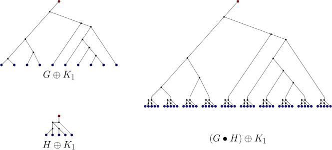
Figure 4: Branch decomposition of $(G\bullet H)\oplus K_{1}$ from the branch decompositions of $G\oplus K_{1}$ and $H\oplus K_{1}$.

Actually the proof of the previous lemma shows that if $G^{\prime}$ is obtained from $G$ by substituting $H$ at some vertex of $G$, then $\operatorname{\mathrm{rw}}(G^{\prime}\oplus K_{1})=\max(\operatorname{\mathrm{rw}}(G\oplus K_{1})$, $\operatorname{\mathrm{rw}}(H\oplus K_{1})$. (The graph $G\bullet H$ is the substitution of $H$ at every vertex of $G$).

Corollary 3.1.

Closing a class by substitution increases the rankwidth by at most one.

For a class $\mathscr{C}$, let $\mathscr{C}\oplus K_{1}$ denote the class $\{G\oplus K_{1}~{}:~{}G\in\mathscr{C}\}$, and let $\mathscr{C}^{\bullet}$ denote the closure of $\mathscr{C}$ under lexicographic product. As a direct consequence of the previous lemma we have

Corollary 3.2.

For every class of graphs $\mathscr{C}$ with bounded rankwidth we have

$$\mathrm{rw}(\mathscr{C})\leq\mathrm{rw}(\mathscr{C}^{\bullet})=\mathrm{rw}(\mathscr{C}\oplus K_{1})\leq\mathrm{rw}(\mathscr{C})+1.$$ (8)

(Indeed, $G\oplus K_{1}\subseteq_{i}G\bullet H$ if $H$ contains at least one edge.)

By substituting each vertex of $V(G)$ in the linear order witnessing $\operatorname{\mathrm{lrw}}(G\oplus K_{1})$ by the linear order of $V(H)$ witnessing $\operatorname{\mathrm{lrw}}(H\oplus K_{1}$) we similarly obtain the following results.

Lemma 3.4.

For all graphs $G,H$ we have

$$\operatorname{\mathrm{lrw}}(G\bullet H)\leq\operatorname{\mathrm{lrw}}(G)+\operatorname{\mathrm{lrw}}(H).$$

Proof.

Let $<_{1}$ be a linear order of $V(G)$ witnessing $\operatorname{\mathrm{lrw}}(G)$ and let $<_{2}$ be a linear order of $V(H)$ witnessing $\operatorname{\mathrm{lrw}}(H)$. Let $<$ be the lexicographic order on $V=V(G)\times V(H)$ defined by $<_{1},<_{2}$, i.e., $(u,v)<(u^{\prime},v^{\prime})$ if $u<u^{\prime}$ or ($u=u^{\prime}$ and $v<v^{\prime}$). Let $t=(u_{t},v_{t})\in V$ and let $(u,v)\leq t$. We have

$$\begin{split}N_{G\bullet H}((u,v))\cap V^{>t}=\big{(}(N_{G}(u)\cap V(G)^{>u_{t}})\times V(H)\big{)}\cup\big{(}\{u_{t}\}\times(N_{H}(v)\cap V(H)^{>v_{t}})\big{)}.\end{split}$$

It follows that the vector space spanned by the sets $N_{G\bullet H}((u,v))\cap V^{>t}$ is in the sum of the vector space spanned by the sets $(N_{G}(u)\cap V(G)^{>u_{t}})\times V(H)$ (which has dimension at most $\operatorname{\mathrm{lrw}}(G)$) and of the vector space spanned by the sets $\{u_{t}\}\times(N_{H}(v)\cap V(H)^{>v_{t}})$ (which has dimension at most $\operatorname{\mathrm{lrw}}(H)$). Hence the claim follows. ∎

3.3 Ramsey properties of rankwidth

In this section we prove that the class of all graphs with rankwidth at most $r+1$ is “Ramsey” for the class of all graphs with rankwidth at most $r$, in the following sense.

Theorem 3.5.

For all integers $r,m$ and every graph $G$ with rankwidth at most $r$ there exists a graph $G^{\prime}=G^{\bullet m}$ with rankwidth $r+1$ and with the property that every $m$-coloring of $G^{\prime}$ contains an induced monochromatic copy of $G$.

Proof.

We define inductively graph $G^{\bullet i}$ for $i\geq 1$: $G^{\bullet 1}=G$ and, for $i\geq 1$ we let $G^{\bullet(i+1)}=G^{\bullet i}\bullet G=G\bullet G^{\bullet i}$. According to Corollary 3.2 we have $\mathrm{rw}(\{G^{\bullet i}~{}:~{}i\in\mathbb{N}\})\leq r+1$.

We prove by induction on $m$ that in every $m$-partition of $G^{\prime}=G^{\bullet m}$ one class induces a subgraph with a copy of $G$. If $m=1$ the result is straightforward. Let $m>1$. Consider a partition $V_{1},\dots,V_{m}$ of the vertex set of $G^{\bullet m}$. If all the copies of $G^{\bullet(m-1)}$ forming $G^{\bullet m}$ contain a vertex in $V_{m}$, then $G^{\bullet m}[V_{m}]$ contains an induced copy of $G$. Otherwise, there is a copy of $G^{\bullet(m-1)}$ in $G^{\bullet m}$ whose vertex set is covered by $V_{1},\dots,V_{m-1}$. By induction hypothesis $G^{\bullet(m-1)}[V_{i}]$ contains an induced copy of $G$. ∎

Corollary 3.3.

Let $\mathscr{F}$ be a proper hereditary class of graphs. Then there exists a class $\mathscr{C}$ with bounded rankwidth such that for every integer $m$ there is $G\in\mathscr{C}$ with the property that for every partition of $V(G)$ into $m$ classes, one class induces a graph not in $\mathscr{F}$.

Corollary 3.4.

The class of graphs with rankwidth at most $2$ does not have the property that its graphs can be vertex partitioned into a bounded number of cographs, or circle graphs, etc.

3.4 Lower bounds for $\chi$-boundedness

Bonamy and Pilipczuk [4] announced independently that classes with bounded rankwidth are polynomially $\chi$-bounded. We give here a lower bound on the degrees of the involved polynomials. We write $\chi_{f}(G)$ for the fractional chromatic number of a graph $G$, which is defined as $\chi_{f}(G)=\inf\bigl{\{}\frac{\chi(G\bullet K_{n})}{n}~{}:~{}n\in\mathbb{N}\bigr{\}}$.

Theorem 3.6.

For $r\in\mathbb{N}$, let $P_{r}$ be a polynomial such that for every graph $G$ with rankwidth at most $r$ we have $\chi(G)\leq P_{r}(\omega(G))$. Then $\deg P_{r}\in\Omega(\log r)$.

Proof.

As shown in [16] for all graphs $G$ and $H$ we have $\chi(G\bullet H)=\chi(G\bullet K_{\chi(H)})$. Furthermore we have $\chi(G\bullet K_{\chi(H)})\geq\chi(H)\chi_{f}(G)$. We deduce that $\chi(G\bullet H)\geq\chi_{f}(G)\chi(H)$. Hence for every integer $n$ we have $\chi(G^{\bullet n})\geq\chi_{f}(G)^{n}$. As $\omega(G^{\bullet n})=\omega(G)^{n}$ we have $\chi(G^{\bullet n})\geq\omega(G^{\bullet n})^{\frac{\log\chi_{f}(G)}{\log\omega(G)}}$ and hence

$$\deg P_{r}\geq\sup_{\mathrm{rw}(G\oplus K_{1})\leq r}\frac{\log\chi_{f}(G)}{\log\omega(G)}.$$

For sufficiently large integers $n$ there exists a triangle-free graph $G_{n}$ with $\chi_{f}(G_{n})\geq\frac{1}{9}\sqrt{\frac{n}{\log n}}$ (see [23]). As $n>\mathrm{rw}(G_{n}\oplus K_{1})$ we deduce that for sufficiently large integers $r$ we have

$$\deg P_{r}\geq\biggl{(}\frac{1}{2\log 2}-o(1)\biggr{)}\log r.$$

∎

Linear rankwidth.

We give a short proof in Section 4 (Corollary 4.1) that classes with bounded linear rankwidth are linearly $\chi$-bounded using the equivalence between classes with bounded linear rankwidth and classes with bounded linear NLC-width. We improve the obtained upper bound of the $\chi/\omega$ ratio in Section 5 using a more technical analysis of linear rank-width (Theorem 5.17), leading to an order of magnitude of $2^{O(r^{2})}$. We now prove that the ratio $\chi/\omega$ can be as large as $\alpha^{r}$ for some constant $\alpha>1$ and for graphs with arbitrarily large linear rankwidth $r$ and clique number $\omega$.

From Lemma 3.4 we deduce $\operatorname{\mathrm{lrw}}(C_{5}^{\bullet n})\leq 2n$. As $\omega(C_{5}^{\bullet n})=2^{n}$ and as $\chi(C_{5}^{\bullet n})\geq\chi(C_{5})\chi_{f}(C_{5})^{n-1}=3(5/2)^{n-1}$ we deduce

$$\frac{\chi(C_{5}^{\bullet n})}{\omega(C_{5}^{\bullet n})}\geq(6/5)(5/4)^{n}\geq(6/5)(5/4)^{\operatorname{\mathrm{lrw}}(C_{5}^{\bullet n})/2}.$$

As $6/5>\sqrt{5}/2$, for every integer $r$ we have:

$$\lim_{t\rightarrow\infty}\ \sup_{\begin{subarray}{c}\operatorname{\mathrm{lrw}}(G)\leq r\\ \omega(G)\geq t\end{subarray}}\ \frac{\chi(G)}{\omega(G)}\geq\biggl{(}\frac{\sqrt{5}}{2}\biggr{)}^{r}.$$ (9)

4 Linear NLC-width

In this section we prove that classes with bounded linear NLC-width (and hence classes of bounded linear rankwdith) are linearly $\chi$-bounded, and if they are stable, then they are transduction equivalent to classes of bounded pathwidth. We prove the result using Simon’s factorization forest theorem.

4.1 Simon’s factorization forest theorem

A semigroup is an algebra with one associative binary operation, usually denoted as multiplication. An idempotent in a semigroup is an element $e$ with $ee=e$. Given an alphabet $\Omega$ we denote by $\Omega^{+}$ the semigroup of all non-empty finite words over $\Omega$, with concatenation as product.

Fix an alphabet $\Omega$ and a semigroup morphism $h\colon\Omega^{+}\rightarrow T$, where $T$ is a finite semigroup. A factorization tree is an ordered rooted tree in which each node is either a leaf labeled by a letter, or an internal node. The value of a node is the word obtained by reading the descendant leaves below from left to right. The value of a factorization tree is the value of the root of the tree. A factorization tree of a word $\alpha\in\Omega^{+}$ is a factorization tree of value $w$. The depth of the tree is defined as usual, with the convention that the depth of a single leaf is $1$. A factorization tree is Ramseyan (for $h$) if every node 1) is a leaf, or 2) has two children, or, 3) the values of its children are all mapped by $h$ to the same idempotent of $T$.

Theorem 4.1 (Simon’s Factorization Forest Theorem [24, 43]).

For every alphabet $\Omega$, every finite semigroup $T$, every semigroup morphism $h\colon\Omega^{+}\rightarrow T$, and every word $\alpha\in\Omega^{+}$, the word $\alpha$ has a Ramseyan factorization tree of depth at most $3|T|$.

The existence of an upper bound expressed only in terms of $|T|$ was first proved by Simon [43]. The improved upper bound of $3|T|$ is due to Kufleitner [24].

4.2 Application to classes with bounded linear NLC-width

In the following we consider the semigroup $\Gamma_{k}$ on functions $r\colon[k]\rightarrow[k]$. Obviously, $h\colon\Omega_{k}(V)^{+}\rightarrow\Gamma_{k}$ induced by $h(a)=r_{a}$ for $a\in\Omega_{k}(V)$ is a semigroup homomorphism (recall Definition 3.1). An idempotent of $\Gamma_{k}$ is a function $r$ that satisfies that if $r(i)=j$, then $r(j)=j$. We call $\alpha\in\Omega_{k}(V)^{+}$ an idempotent if $h(\alpha)$ is an idempotent in $\Gamma_{k}$.

For $\alpha\in\mathfrak{L}_{k}(V)$ (recall Definition 3.2) and for a letter $a$ of $\alpha$ and $v=v_{a}$ define $\mathrm{col}_{\alpha}(v)$ as the color of the vertex $v$ in $\Xi(\alpha)$. Note that if $\alpha\beta\in\mathfrak{L}_{k}(V)$ then $\mathrm{col}_{\alpha\beta}(v)=h(\beta)(\mathrm{col}_{\alpha}(v))$.

Fix $\alpha\in\mathfrak{L}_{k}(V)$. According to Theorem 4.1, there exists a rooted tree $Y$ that is a Ramseyan factorization tree of $\alpha$ for $h$ with depth at most $3|T|$. We identify the vertices of $\Xi(\alpha)$ with the leaves of $Y$. Let $z$ be a letter of $\Xi(\alpha)$ and let $\beta$ be an ancestor of $z$. Let $\beta=b_{1}\dots b_{n}$ (where the $b_{i}$ are letters) and let $p\leq n$ be such that $b_{p}=z$. We define

$$\mathrm{recol}_{\beta}(z) =r_{b_{p-1}}\circ\dots\circ r_{b_{1}},$$

$$\mathrm{eset}_{\beta}(z) =\mathrm{recol}_{\beta}(z)^{-1}(e_{z}).$$

Lemma 4.2.

Let $z_{1},z_{2}$ be two letters of $\alpha$ appearing in this order in $\alpha$, let $\beta$ be their least common ancestor, and let $\delta_{1}$ (resp. $\delta_{2}$) be the children of $\beta$ containing the letter $z_{1}$ (resp. $z_{2}$). Then $v_{z_{1}}$ and $v_{z_{2}}$ are adjacent in $\Xi(\alpha)$ if

• $\delta_{1}$ is not immediately to the left of $\delta_{2}$ in $\alpha$ and $\mathrm{col}_{\beta}(z_{1})\in\mathrm{eset}_{\beta}(z_{2})$, or

• $\delta_{1}$ is immediately to the left of $\delta_{2}$ in $\alpha$ and $\mathrm{col}_{\delta_{1}}(z_{1})\in\mathrm{eset}_{\beta}(z_{2})$.

Proof.

When $\delta_{1}$ and $\delta_{2}$ are consecutive, let $\delta_{2}=b_{1}\dots b_{p}$ with $b_{p}=z_{2}$. Then $v_{z_{1}}$ and $v_{z_{2}}$ are adjacent if

$$\mathrm{col}_{\delta_{1}b_{1}\dots b_{p-1}}(z_{1})\in e_{z_{2}}$$

$$\iff\quad \mathrm{recol}_{\beta}(\mathrm{col}_{\delta_{1}}(z_{1}))\in e_{z_{2}}$$

$$\iff\quad \mathrm{col}_{\delta_{1}}(z_{1})\in\mathrm{eset}_{\beta}(z_{2}).$$

(Note that in this case we do not make any assumption on $h(\delta_{1})$ and $h(\delta_{2})$.)

Now assume that $\delta_{1}$ and $\delta_{2}$ are non-consecutive. Let $\beta_{1},\dots,\beta_{n}$ be the children of $\beta$, and let $j\geq i+2$ be such that $\delta_{1}=\beta_{i}$ and $\delta_{2}=\beta_{j}$. As $\beta$ has more than two children, the corresponding factorization is a factorization into idempotents. Let $r=h(\beta_{1})=\dots=h(\beta_{n})$. Let $\delta_{2}=b_{1}\dots b_{p}$ with $b_{p}=z_{2}$.

Then $v_{z_{1}}$ and $v_{z_{2}}$ are adjacent if

$$\mathrm{col}_{\beta_{i}\dots\beta_{j-1}b_{1}\dots b_{p-1}}(z_{1})\in e_{z_{2}}$$

$$\iff\quad \mathrm{recol}_{\beta}(\mathrm{col}_{\beta_{i}\dots\beta_{j-1}}(z_{1})))\in e_{z_{2}}$$

$$\iff\quad \mathrm{col}_{\beta_{i}\dots\beta_{j-1}}(v_{z_{1}})\in\mathrm{eset}_{\beta}(z_{2})$$

$$\iff\quad r^{j-i-1}(\mathrm{col}_{\beta_{i}}(z_{1}))\in\mathrm{eset}_{\beta}(z_{2})$$

$$\iff\quad r^{n-i-1}(\mathrm{col}_{\beta_{i}}(z_{1}))\in\mathrm{eset}_{\beta}(z_{2})$$

$$\iff\quad \mathrm{col}_{\beta_{i}\dots\beta_{n}}(z_{1})\in\mathrm{eset}_{\beta}(z_{2})$$

$$\iff\quad \mathrm{col}_{\beta}(z_{1})\in\mathrm{eset}_{\beta}(z_{2})$$

∎

Theorem 4.3.

Let $f(k)=(k2^{k+1})^{3k^{k}}$ and $g(k)=3k^{k}$. Every graph with linear NLC-width at most $k$ can be vertex partitioned into $f(k)$ cographs with a cotree of depth at most $g(k)$.

Proof.

Let $\kappa$ be a coloring of the nodes $\beta$ with color in $[2]$ such that two consecutive children of a node have a different color. For a letter $z$ of $\alpha$, color $v_{z}$ by the vector of values $(\kappa(\beta),\mathrm{col}_{\beta}(z),\mathrm{eset}_{\beta}(z))$ for $\beta$ ancestor of $z$. (This gives a vector of at most $3|T|$ triples). Consider a monochromatic subset of vertices. It is easily checked that this set induces a cograph with cotree height at most $3|T|$. ∎

Corollary 4.1.

Classes with bounded linear NLC-width are linearly $\chi$-bounded.

Lemma 4.4.

Assume there exists $\beta$ and letters $x_{1},y_{1},x_{2},y_{2},\dots,x_{\ell},y_{\ell}$ of $\beta$ (in this order) such that $\beta$ is the least common ancestor of each pair of these letters, and that there exist $c_{x},c_{y}\in[k]$ and $e_{x},e_{y}\subseteq[k]$ with $c_{x}\in e_{y},c_{y}\notin e_{x}$, and, for each $1\leq i\leq\ell$, $\mathrm{col}_{\beta}(x_{i})=c_{x}$, $\mathrm{eset}_{\beta}(x_{i})=e_{x}$, $\mathrm{col}_{\beta}(y_{i})=c_{y}$, and $\mathrm{eset}_{\beta}(x_{y})=e_{y}$. Then $\Xi(\alpha)$ contains a semi-induced half-graph of order at least $\lfloor\ell/3\rfloor$.

Proof.

By taking at least a third of the indices we can assume that no two letters appear in consecutive children of $\beta$. Then it follows directly from Lemma 4.2 that these vertices semi-induce a half-graph. ∎

Theorem 4.5.

Let $\mathscr{C}$ be a class with bounded linear NLC-width. If the graphs in $\mathscr{C}$ exclude some semi-induced half-graph, then $\mathscr{C}$ is a transduction of a class with bounded pathwidth.

Proof.

We first construct the interval graph $H$, where each node $\delta$ of $Y$ corresponds to an interval $I_{\delta}$. The descendent relation of $Y$ is then the containment relation in the set of intervals.

Now consider an internal node $\delta$ of $Y$ and a $4$-tuple $(c_{1},e_{1},c_{2},e_{2})\in[k]\times 2^{[k]}\times[k]\times 2^{[k]}$ with $c_{1}\in e_{2}$ and $c_{2}\notin e_{1}$, such that at least one descendent $z_{1}$ of $\delta$ is such that $\mathrm{col}_{\delta}(z_{1})=c_{1}$ and $\mathrm{col}_{\delta}(z_{1})=e_{1}$ and at least one descendent $z_{2}$ of $\delta$ is such that $\mathrm{col}_{\delta}(z_{1})=c_{2}$ and $\mathrm{col}_{\delta}(z_{1})=e_{2}$. We consider new intervals coming from the split of the $I_{\delta}$ into subintervals: These subintervals are obtained by considering the children of $\delta$ in order. The subintervals are of three types:

• the type $(1)$ contain consecutive children with at least one children with $\mathrm{col}_{\delta}(z)=c_{1}$ and $\mathrm{col}_{\delta}(z)=e_{1}$, but no descendant $z$ with $\mathrm{col}_{\delta}(z)=c_{2}$ and $\mathrm{col}_{\delta}(z)=e_{2}$;

• the type $(2)$ contain consecutive children with at least one children with $\mathrm{col}_{\delta}(z)=c_{2}$ and $\mathrm{col}_{\delta}(z)=e_{2}$, but no descendant $z$ with $\mathrm{col}_{\delta}(z)=c_{1}$ and $\mathrm{col}_{\delta}(z)=e_{1}$;

• the type $(1+2)$ contains a single children with both a descendent $z_{1}$ with $\mathrm{col}_{\delta}(z_{1})=c_{1}$ and $\mathrm{col}_{\delta}(z_{1})=e_{1}$ and a descendent $z_{2}$ with $\mathrm{col}_{\delta}(z_{1})=c_{2}$ and $\mathrm{col}_{\delta}(z_{1})=e_{2}$.

The division of $I_{\delta}$ into subintervals is done in such a way that no two consecutive subintervals are both of type $(1)$ or both of type $(2)$. Note that such a division into subintervals, though not uniquely defined, always exists.

Assume that the number of subintervals into which we divided $I_{\delta}$ is $N$. Then we can select, among the descendants of the distinct children of $\delta$ some vertices $\alpha_{1},\beta_{1},\dots,\alpha_{n},\beta_{n}$ (with $n\geq N/4$) such that $\mathrm{col}_{\delta}(\alpha_{i})=c_{1}$, $\mathrm{col}_{\delta}(\alpha_{i})=e_{1}$, $\mathrm{col}_{\delta}(\beta_{i})=c_{2}$, and $\mathrm{col}_{\delta}(\beta_{i})=e_{2}$. It is easily checked that the vertices $\alpha_{1},\beta_{1},\dots$, $\alpha_{n},\beta_{n}$ semi-induce a half-graph of order $n$. As $\mathscr{C}$ excludes some semi-induced half-graph we deduce that $I_{\delta}$ is divided into a bounded number of subintervals, which can be numbered using a bounded number of unary predicates.

Let $u,v$ be vertices, and let $\delta$ be their least common ancestor in $Y$. The values of $\mathrm{col}_{\delta}$ and $\mathrm{eset}_{\delta}$ for $u$ and $v$ are known from the predicates at these vertices. Let $c_{1}=\mathrm{col}_{\delta}(u)$, $e_{1}=\mathrm{eset}_{\delta}(u)$, $c_{2}=\mathrm{col}_{\delta}(v)$, and $e_{2}=\mathrm{eset}_{\delta}(v)$. If $c_{1}\in e_{2}$ and $c_{2}\in e_{1}$ then $u$ and $v$ are adjacent. If $c_{1}\notin e_{2}$ and $c_{2}\notin e_{1}$ then $u$ and $v$ are non-adjacent. In the last case, without loss of generality, we can assume $c_{1}\in e_{2}$ and $c_{2}\notin e_{1}$.

The two vertices $u$ and $v$ cannot belong to a same subinterval of $I_{\delta}$. From the numbering marks associated to the subintervals that contain $u$ and $v$ we deduce which of $u$ and $v$ is smaller than the other and hence the adjacency between $u$ and $v$. ∎

From this we deduce.

Theorem 4.6.

Let $\mathscr{C}$ be a class of graphs with linear rankwidth at most $r$. Then the following are equivalent:

1. $\mathscr{C}$ is stable,

2. $\mathscr{C}$ is monadically stable,

3. $\mathscr{C}$ is sparsifiable,

4. $\mathscr{C}$ has $2$-covers with bounded shrubdepth,

5. $\mathscr{C}$ has structurally bounded expansion,

6. $\mathscr{C}$ is a transduction of a class with bounded pathwidth,

7. $\mathscr{C}$ excludes some semi-induced half-graph.

5 Linear rankwidth

In this section we present a second proof for the result that classes with bounded linear rankwidth are linearly $\chi$-bounded and thereby provide improved constants.

5.1 Notation

For sets $M,N\subseteq V(G)$ we define $M\oplus N$ as the symmetric difference of $M$ and $N$, that is, $v\in M\oplus N$ if and only if $v\in M\cup N$ but $v\notin M\cap N$. For $t\in V$, we define $V^{>t}\coloneqq\{v:v>t\}$, $V^{<t}\coloneqq\{v:v<t\}$ and $V^{\leq t}\coloneqq\{v:v\leq t\}$. For $v\in V$ we denote by $N(v)$ the neighborhood of $v\in G$ (where $v$ not included). We let $N^{<t}(v)\coloneqq N(v)\cap V^{<t}$ and define similarly $N^{>t}$ and $N^{\leq t}$. For $M\subseteq V(G)$ we define $N_{\oplus}(M)\coloneqq\bigoplus_{v\in M}N(v)$ and $N_{\oplus}^{>t}(M)\coloneqq N_{\oplus}(M)\cap V^{>t}$.

Remark 5.1.

If $t<t^{\prime}$, then $N_{\oplus}^{>t}(M)=N_{\oplus}^{>t}(N)$ implies $N_{\oplus}^{>t^{\prime}}(M)=N_{\oplus}^{>t^{\prime}}(N)$.

For $t\in V$ the closure of $\{N^{>t}(v):v\leq t\}$ under $\oplus$ is a vector space over $\oplus$ and scalar multiplication with $0$ and $1$, where $0\cdot M=\emptyset$ and $1\cdot M=M$.

For $t\in V$, we call an inclusion-minimal subset $B\subseteq V_{\leq t}$ a neighbor basis for $V^{>t}$ if for every $v\leq t$ there exists $B^{\prime}\subseteq B$ such that $N^{>t}(v)=N_{\oplus}^{>t}(B^{\prime})$. In other words, $B$ is a neighbor basis for $V^{>t}$ if $\{N^{>t}(v)~{}:~{}v\in B\}$ forms a basis for the space spanned by $\{N^{>t}(v)~{}:~{}v\leq t\}$.

The following is immediate by the definition of linear rankwidth.

Remark 5.2.

As $G$ has linear rankwidth at most $r$, for every $t\in V$ every neighbor basis for $V^{>t}$ of order at most $r$.

5.2 Activity intervals and active basis

For $t\in V$ we define the active basis $B_{t}$ at $t$ as the set

$$B_{t}=\{v\leq t~{}:~{}(\nexists B\subseteq V^{<v})\ N^{>t}(v)=N_{\oplus}^{>t}(B)\}.$$ (10)

Note that this is the lexicographically least neighborhood basis of $V^{>t}$.

Remark 5.3.

If the linear order of $V(G)$ is given, the set of all neighborhood basis $B_{t}$ for $t\in V(G)$ can be computed in linear time.

To each $v\in V$ we associate its activity interval $I_{v}$ defined as the interval $[v,\tau(v)]$ starting at $v$ and ending at the minimum vertex $\tau(v)\geq v$ such that $v\notin B_{\tau(v)}$. Note that $\tau(v)$ is well defined as we have $B_{\max V}=\emptyset$.

We extend the definitions of the activity intervals and of the $\tau$ function to all subsets $M$ of $V(G)$ by

$$I_{M}\coloneqq\bigcap_{v\in M}I_{v}\quad\text{ and }\quad\tau(M)=\min_{v\in M}\tau(v).$$ (11)

Note that either $I_{M}=\emptyset$ or $I_{M}=[\max M,\tau(M)]$. We call a set $M$ active if $|I_{M}|>1$, that is, if $\max M<\tau(M)$. We call a vertex $v$ active if the singleton set $\{v\}$ is active.

For every $v\in V$, as $v\notin B_{\tau(v)}$, there exists a unique $F_{0}(v)\subseteq B_{\tau(v)}$ with

$$N^{>\tau(v)}(v)=N_{\oplus}^{>\tau(v)}(F_{0}(v)).$$ (12)

Note that if $F_{0}(v)\neq\emptyset$, then we have

$$\max F_{0}(v)<v\leq\tau(v)<\tau(F_{0}(v)).$$ (13)

Hence, in this case, the set $F_{0}(v)$ is active.

Remark 5.4.

Assume that $M$ is an active set and let $v\in M$.

1. If $\tau(v)>\tau(M)$, then $v\in B_{\tau(M)}$.

2. If $\tau(v)=\tau(M)$, then $F_{0}(v)\subseteq B_{\tau(M)}$.

5.3 The F-tree

We define a mapping $F$ extending $F_{0}$, that will define a rooted tree on the set $Z$ consisting of all active sets, all singleton sets $\{v\}$ for $v\in V(G)$, and $\emptyset$ (which will be the root of the tree and the unique fixed point of $F$). Before we define $F$ we make one more observation.

Lemma 5.5.

Let $u,v\in V(G)$ be active. If $\tau(u)=\tau(v)$, then $u=v$.

Proof.

Let $t=\tau(u)=\tau(v)$ and let $t^{\prime}$ be the predecessor of $t$ in the linear order. Assume for contradiction that $u\neq v$. By definition of $F_{0}$ we have $N^{>t}(u)=N^{>t}(F_{0}(u))$ and $N^{>t}(v)=N^{>t}(F_{0}(v))$. We have $N^{>t^{\prime}}(u)\neq N^{>t^{\prime}}(F_{0}(u))$ as otherwise $\tau(u)\leq t^{\prime}$. As $N^{>t^{\prime}}(u)\oplus N^{t}(u)\subseteq\{t\}$ and $N^{>t^{\prime}}(F_{0}(u))\oplus N^{t}(F_{0}(u))\subseteq\{t\}$, we have $N^{>t^{\prime}}(F_{0}(u))=N^{>t^{\prime}}(u)\oplus\{t\}$. Similarly, we have $N^{>t^{\prime}}(F_{0}(v))=N^{>t^{\prime}}(v)\oplus\{t\}$. Assume without loss of generality that $u<v$. Then $N^{>t^{\prime}}(v)=N^{>t^{\prime}}(\{u\})\oplus N^{>t^{\prime}}(F_{0}(u))\oplus N^{>t^{\prime}}(F_{0}(v))$. As $\max(\{u\}\cup F_{0}(u)\cup F_{0}(v))<v$ we deduce that $\tau(v)\leq t^{\prime}$, contradicting $\tau(v)=t$. ∎

Corollary 5.1.

For each active set $M\subseteq V(G)$ there exists exactly one $v\in M$ with $\tau(v)=\tau(M)$.

The mapping $F\colon Z\rightarrow Z$ is defined as

$$F(M)=\begin{cases}\emptyset&\text{if }M=\emptyset,\\ M\oplus\{v\}\oplus F_{0}(v)&\text{for the unique $v\in M$}\\ &\text{with $\tau(v)=\tau(M)$, otherwise}.\end{cases}$$ (14)

Remark 5.6.

If the linear order on $V(G)$ is given then $F$-mapping on $Z$ can be computed in linear time. (Note that $|Z|\leq 2^{r}|V(G)|$.)

The following lemma shows for every active set $M$, either $F(M)=\emptyset$ or $F(M)$ is active, and thus $F(M)\in Z$ and $F$ is well defined. Furthermore, the lemma shows that $I_{F(M)}\supset I_{M}$.

Lemma 5.7.

Let $M\in Z$. Then $F(M)\subseteq B_{\tau(M)}$ and furthermore, either $F(M)=\emptyset$, or $\max F(M)\leq\max M<\tau(M)<\tau(F(M))$ and hence $F(M)$ is active.

Proof.

The statement is obvious if $M=\emptyset$. For $M=\{v\}$, the statement is immediate from the definition of $F_{0}(v)$ and eq. 13. For all other $M\in Z$, according to remark 5.4 we have for each $v\in M$ either $v\in B_{\tau(M)}$ if $\tau(v)>\tau(M)$, or $F_{0}(v)\subseteq B_{\tau(M)}$ if $\tau(v)=\tau(M)$. This implies $F(M)\subseteq B_{\tau(M)}$. Finally, if $F(M)\neq\emptyset$, then $\max F(M)\leq\max M<\tau(M)<\tau(F(M))$ follows from the fact that these inequalities hold for all $v\in M$ with $\tau(v)>\tau(M)$ and for $F_{0}(v)$ for the unique $v\in M$ with $\tau(v)=\tau(M)$ according to eq. 13. ∎

The mapping $F$ guides the process of iterative referencing and ensures that, for an active set $M$, if $t\geq\tau(M)$, then the set $N_{\oplus}^{>t}(M)$ can be rewritten as $N_{\oplus}^{>t}(F(M))$. This property is stated in the next lemma.

Lemma 5.8.

Let $M\in Z\setminus\{\emptyset\}$ and let $w\in V(G)$. If $w>\tau(M)$, then

$$w\in N_{\oplus}(M)\Leftrightarrow w\in N_{\oplus}(F(M)).$$

Proof.

If $M=\{v\}$ for $v\in V(G)$, then this follows from (12). Otherwise, $M$ is an active set. Let $t=\tau(M)$ and let $v\in M$ be the unique element with $\tau(v)=t$. Then we have $N_{\oplus}^{>t}(F(v))=N_{\oplus}^{>t}(v)$, and hence

$$N_{\oplus}^{>t}(F(M)) =N_{\oplus}^{>t}(\{v\})\oplus N_{\oplus}^{>t}(F(M)\oplus\{v\})$$

$$=N_{\oplus}^{>t}(F_{0}(v))\oplus N_{\oplus}^{>t}(F(M)\oplus\{v\})$$

$$=N_{\oplus}^{>t}(M).$$

∎

This lemma can be applied repeatedly to $M,F(M),$ etc. until $F^{k}(M)=\emptyset$, or until for some given $w\in V(G)$ we have $\tau(F^{k}(M))\geq w$. This justifies to introduce, for distinct vertices $u$ and $v$ the value

$$\xi(u,v):=\min\{k~{}:~{}v\in I_{F^{k}(u)}\text{ or }F^{k}(u)=\emptyset\}$$ (15)

As a direct consequence of the previous lemma we have

Corollary 5.2.

For distinct $u,v\in V(G)$ we have

$$\{u,v\}\in E(G)\Longleftrightarrow\begin{cases}v\in N_{\oplus}(F^{\xi(u,v)}(u))&\text{if }u<v,\\ u\in N_{\oplus}(F^{\xi(v,u)}(v))&\text{if }u>v.\end{cases}$$

Proof.

As the two cases are symmetric, we can assume $u<v$. If $k=0$, then the statement is $\{u,v\}\in E(G)\Leftrightarrow v\in N_{\oplus}(u)$, which trivially holds. Assume $\xi(u,v)=k\geq 1$. By Lemma 5.7 we have $v>\tau(F^{k-1}(\{u\}))>\tau(F^{k-2}(\{u\}))>\dots>\tau(u)$. Moreover, $u,F(\{u\}),\dots,F^{k-1}(\{u\})\in Z\setminus\{\emptyset\}$. Hence by Lemma 5.8 we have

$$\{u,v\}\in E(G) \Leftrightarrow v\in N_{\oplus}(u)$$

$$\Leftrightarrow v\in N_{\oplus}(F(\{u\}))$$

$$\Leftrightarrow v\in N_{\oplus}(F^{2}(\{u\}))\Leftrightarrow\ldots$$

$$\Leftrightarrow v\in N_{\oplus}(F^{k}(\{u\})).$$

∎

The monotonicity property of $F$ (i.e. the property $\tau(F(M))>\tau(M)$ if $F(M)\neq\emptyset$) implies that $F$ defines a rooted tree, the $F$-tree, with vertex set $Z$, root $\emptyset$ and edges $\{M,F(M)\}$. Here the monotonicity guarantees that the graph is acyclic and it is connected because $\emptyset$ is the only fixed point of $F$. The following lemma shows that the $F$-tree has bounded height. Recall that $r$ denotes the linear rankwidth of $G$.

Lemma 5.9.

For every $M\in Z$ we have $F^{r+1}(M)=\emptyset$.

Proof.

If $M=\emptyset$, the statement is obvious, so assume $M\neq\emptyset$. It is sufficient to prove that for every active set $M$ we have $F^{r}(M)=\emptyset$, as this implies $F^{r+1}(\{v\})=\emptyset$ also for all $v\in V(G)$. Let $M$ be an active set and let $t\in I_{M}$. Then every $v\in M$ is in $B_{t}$, so $M\subseteq B_{t}$.

Assume $i\geq 1$ is such that $F^{i}(M)\neq\emptyset$. As $\max F(M)\leq\max M$ and $\tau(F(M))>\tau(M)$ by Lemma 5.7, we get

$$\max F^{i}(M)\leq\max M\leq t<\tau(M)\leq\tau(F^{i-1}(M))<\tau(F^{i}(M)).$$

As $\tau(F^{i}(M))=\min_{v\in F^{i}(M)}\tau(v)$, we have $F^{i}(M)\subseteq B_{t}$. Hence, considering the sequence $M,F(M),\dots,F^{i}(M)$, each iteration of $F$ removes the unique element with minimum $\tau$ value. It follows that the union of the sets has cardinality at least $i+1$. As $|B_{t}|\leq r$, we have $i<r$ and hence $F^{r}(M)=\emptyset$. ∎

For distinct vertices $u,v$, let $u\wedge v$ denote the greatest common ancestor of $u$ and $v$ in the $F$-tree, i.e. the first common vertex on the paths to the root. Then there exist $\ell_{u}$ and $\ell_{v}$ such that $u\wedge v=F^{\ell_{u}}(u)=F^{\ell_{v}}(v)$, hence both $u$ and $v$ belong to $I_{u\wedge v}$. Thus we have $\tau(u\wedge v)>u$ and $\tau(u\wedge v)>v$. In other words, we have $\xi(u,v)\leq\ell_{u}$ and $\xi(v,u)\leq\ell_{v}$.

5.4 The activity interval graph

Let $H$ be the intersection graph of the intervals $I_{v}$ for $v\in V(G)$. Note that we may identify $V(H)$ with $V(G)$ as $\min I_{v}=v$ for all $v\ V(G)$.

Lemma 5.10.

The intersection graph $H$ of the intervals $I_{u}$ has pathwidth at most $r+1$, i.e. at most $r+2$ intervals intersect in each point.

Proof.

Consider any vertex $t$ with $t\in I_{u}$ for some $u$. The case $u\in B_{t}$ gives a maximum of $r$ intervals intersecting in $t$. Otherwise $t=\tau(u)$, which gives at most two possibilities for $u$: either $u$ is inactive (and $u=t$), or $u$ is active (and $u$ is uniquely determined, according to lemma 5.5). Thus at most $r+2$ intervals intersect at point $t$. ∎

As mentioned in the proof of the above lemma, every clique of $H$ contains at most one inactive vertex. It follows that there is a coloring $\gamma\colon V(G)\rightarrow[r+2]$ with the following properties:

1. for every $u\in V(G)$ we have $\gamma(u)=r+2$ if and only if $u$ is inactive;

2. for all distinct $u,v\in V(G)$ we have

   $$I_{u}\cap I_{v}\neq\emptyset\quad\Longrightarrow\quad\gamma(u)\neq\gamma(v).$$ (16)

We extend this coloring to sets as follows: for $M\subseteq V(G)$ we let

$$\Gamma(M)\coloneqq\{\gamma(v)~{}:~{}v\in M\}.$$ (17)

This coloring allows to define, for each $v\in V(G)$

$$\operatorname{\mathrm{Class}}(v) \coloneqq\big{(}\gamma(v),\Gamma(F(v)),\dots,\Gamma(F^{r}(v))\big{)},$$

$$\operatorname{\mathrm{NCol}}(v) \coloneqq\{\gamma(u)~{}:~{}u\in N(v)\text{ and }v\in I_{u}\}$$

Note that all $u$ with $v\in I_{u}$ define a clique of $H$ (because all $I_{u}$ contain $v$) and hence have distinct $\gamma$-colors.

Lemma 5.11.

Let $v\in V(G)$. Every $u\in B_{v}$ can be defined as the maximum vertex $x\leq v$ with $\gamma(x)=\gamma(u)$.

Proof.

By assumption we have $u\leq v$. Assume towards a contradiction that there exists $x\in V(G)$ with $u<x\leq v$ and $\gamma(x)=\gamma(u)$. As $u\in B_{v}$ we have $\tau(u)>v$, hence $x\in I_{u}$. It follows that $I_{x}\cap I_{u}\neq\emptyset$, in contradiction to $\gamma(x)=\gamma(u)$. ∎

Towards the aim of bounding the number of graphs of linear rankwidth at most $r$, we give a bound on the number of colors that can appear.

Lemma 5.12.

Let $f(r)\coloneqq 3(r+2)!\,2^{\binom{r+1}{2}}$. The number of pairs $(\operatorname{\mathrm{Class}}(v),\operatorname{\mathrm{NCol}}(v))$ for $v\in V(G)$ can be bounded by $f(r)$.

Proof.

Let $v\in V(G)$. From the fact that $\gamma(v)=r+2$ if and only if $v$ is inactive, that images by $F$ only contain active vertices, as well as from lemma 5.7 we deduce:

• If $\gamma(v)=r+2$, then there exists a linear order on $[r+1]$ colors such that for $1\leq i\leq r$, the set $\Gamma(F^{i}(v))$ is a subset of the first $r+1-i$ colors of $[r+1]$.

• If $\gamma(v)\leq r+1$, then there exists a linear order on $[r+1]\setminus\{\gamma(v)\}$ such that for $1\leq i\leq r$, the set $\Gamma(F^{i}(v))$ is a subset of the first $r-i$ colors of $[r]$.

Thus the number of distinct $\operatorname{\mathrm{Class}}(v)$ for $v\in V(G)$ is bounded by

$$(r+1)!\,2^{r}2^{r-1}\dots 2+(r+1)r!\,2^{r-1}\dots 2=3(r+1)!\,2^{\binom{r}{2}}.$$

Furthermore, the number of distinct $\operatorname{\mathrm{NCol}}(v)$ for $v\in V(G)$ is at most $(r+2)2^{r+1}$. ∎

5.5 Encoding the graph in the linear order

We first make use of Corollary 5.2 to encode $G$ by a first-order formula using only the newly added colors and the order $<$ on $V(G)$. More precisely, for $v\in V(G)$, let

$$\operatorname{\mathrm{ICol}}(v)\coloneqq\{\gamma(u)~{}:~{}v\in I_{u}\}.$$

Let $\mathcal{L}$ be the structure over signature $\Lambda\mathbin{\cup}\{<\}$, where $\Lambda$ is the set of all colors of the form $(\operatorname{\mathrm{Class}}(v),\operatorname{\mathrm{NCol}}(v),\operatorname{\mathrm{ICol}}(v))$, with the same elements as $G$ and $<$ interpreted as in $G$. Every element $v$ of $\mathcal{L}$ is equipped with the color $(\operatorname{\mathrm{Class}}(v),$ $\operatorname{\mathrm{NCol}}(v),\operatorname{\mathrm{ICol}}(v))$. The following lemma gives a new proof of the result of [5].

Lemma 5.13.

There exists an $\exists\forall$-first-order formula $\varphi(x,y)$ over the vocabulary $\Lambda\mathbin{\cup}\{<\}$ such that for all $u,v\in V(G)$ we have

$$\mathcal{L}\models\varphi(u,v)\Longleftrightarrow\{u,v\}\in E(G).$$

Proof.

By symmetry, we can assume that $u<v$. According to corollary 5.2 for distinct $u,v\in V(G)$ we have

$$\{u,v\}\in E(G)\Longleftrightarrow\begin{cases}v\in N_{\oplus}(F^{\xi(u,v)}(u))&\text{if }u<v\\ u\in N_{\oplus}(F^{\xi(v,u)}(v))&\text{if }u>v.\end{cases}$$

Note that we can extract any color from $\Lambda$, i.e. we can define $\gamma(x)\in\Gamma(F^{i}(y))$ and $\gamma(x)\in\operatorname{\mathrm{ICol}}(y)$. For example, $\gamma(x)\in\Gamma(F^{i}(y))$ is a big disjunction over all possible colorings $\Lambda(x)=(\operatorname{\mathrm{Class}}(x),NC(x),\operatorname{\mathrm{ICol}}(x))$ and $\Lambda(y)=(\operatorname{\mathrm{Class}}(y),NC(y),\operatorname{\mathrm{ICol}}(y))$ satisfying that $\operatorname{\mathrm{Class}}(x)$ has in its first component an element from the $i$th component of $\operatorname{\mathrm{Class}}(y)$.

We first define formulas $\psi^{i}(x,y)$ such that for all $u,v\in V(G)$

$$\mathcal{G}\models\psi^{i}(u,v)\Leftrightarrow v\in F^{i}(u).$$

Let $C=\Gamma(F^{i}(u))$. According to lemma 5.11, for $a\in C$, the element of $F^{i}(u)\subseteq B_{u}$ with color $a$ is the maximal element $w<u$ such that $\gamma(w)=a$. The formula can express that $y<x$ is maximal with $\gamma(y)=a$ by $(y<x)\wedge(\gamma(y)=a)$ $\wedge\forall z\,((z>y)\wedge(z<x)\rightarrow\gamma(z)\neq a)$. Here, for convenience, we use $\gamma(z)=a$ as an atom. Note that $\psi^{i}(x,y)$ is a $\forall$-formula.

We now define formulas $\alpha^{k}(x,y)$ such that for all $u,v\in V(G)$ with $u<v$ we have

$$\mathcal{G}\models\alpha^{k}(u,v)\Leftrightarrow k=\xi(u,v).$$

Observe that $v\in I_{F^{k}(u)}$ if and only if for every $x\in F^{k}(u)$ we have $x\leq v$, $a\in\operatorname{\mathrm{ICol}}(v)$ (i.e. there exists some $y$ with $\gamma(y)=a$ and $v\in I_{y}$) and there exists no $z$ with $x<z\leq v$ with $\gamma(z)=a$ (hence $\min I_{y}\leq x$, which implies that $I_{y}$ and $I_{x}$ intersects thus $x=y$ as $\gamma(x)=\gamma(y)$). We restrict ourselves to the case $u<v$ and obtain

$$\begin{split}u<v\land v\in I_{F^{k}(u)}\iff u<v\land{}&\Gamma(F^{k}(u))\subseteq\operatorname{\mathrm{ICol}}(v)\\ {}\land&\forall x\,(x\in F^{k}(u)\mathbin{\rightarrow}x\leq v\land\gamma(x)\notin\operatorname{\mathrm{ICol}}(v))\,.\end{split}$$

Then $\xi(u,v)$ for $u<v$ is the minimum integer $k$ such that $v\in I_{F^{k}(u)}$ or $F^{k}(u)=\emptyset$, and this is easy to state as a $\forall$-formula. Finally, if we have determined $\xi(u,v)$, with the help of the formulas $\psi^{i}$ we can determine whether $\{u,v\}\in E(G)$ as in the proof of corollary 5.2 by existentially quantifying the elements of $F(u),F^{2}(u),\ldots,F^{\xi(u,v)}(u)$ and expressing whether $v\in N_{\oplus}(F^{\xi(u,v)}(u))$. Indeed, for every $x\in F^{\xi(u,v)}(u)$ we have $v\in I_{F^{\xi(u,v)}(u)}\subseteq I_{x}$, hence the adjacency of $x$ and $y$ is encoded in $\operatorname{\mathrm{NCol}}(v)$.

This information can hence be retrieved by an $\exists\forall$-formula, as claimed. ∎

Lemma 5.14.

Let $f^{\prime}(r)\coloneqq(r+2)!\,2^{\binom{r}{2}}3^{r+2}$. The number of triples $(\operatorname{\mathrm{Class}}(v),\operatorname{\mathrm{NCol}}(v),\operatorname{\mathrm{ICol}}(v))$ for $v\in V(G)$ can be bounded by $f^{\prime}(r)$.

Proof.

In Lemma 5.12 we have shown that the number of distinct $\operatorname{\mathrm{Class}}(v)$ for $v\in V(G)$ is bounded by $3(r+1)!\,2^{\binom{r}{2}}$. The number of pairs $(\operatorname{\mathrm{NCol}}(v),\operatorname{\mathrm{ICol}}(v))$ is at most $(r+2)3^{r+1}$ (for each color $a$ in $[r+1]$ either $a\notin\operatorname{\mathrm{ICol}}(v)$ or $a\in\operatorname{\mathrm{ICol}}(v)\setminus\operatorname{\mathrm{NCol}}(v)$ or $a\in\operatorname{\mathrm{NCol}}(v)$). ∎

As a corollary we conclude an upper bound on the number of graphs of bounded linear rankwidth.

Theorem 5.15.

Unlabeled graphs with linear rankwidth at most $r$ can be encoded using at most $\binom{r}{2}+r\log_{2}r+\log_{2}(3/e)r+O(\log_{2}r)$ bits per vertex. Precisely, the number of unlabelled graphs of order $n$ with linear rankwidth at most $r$ is at most $\left[(r+2)!\,2^{\binom{r}{2}}3^{r+2}\right]^{n}$.

Remark 5.16.

The encoding can be computed in linear time if the linear order on $G$ is given.

5.6 Partition into cographs

Theorem 5.17.

Let $f(r)=3(r+2)!\,2^{\binom{r+1}{2}}$. The $c$-chromatic number of every graph $G$ is bounded by $f(\operatorname{\mathrm{lrw}}(G))$ and hence

$$\chi(G)\leq f(\operatorname{\mathrm{lrw}}(G))\,\omega(G).$$ (18)

Proof.

Let $u\sim v$ hold if and only if $\operatorname{\mathrm{Class}}(u)=\operatorname{\mathrm{Class}}(v)$ and $\operatorname{\mathrm{NCol}}(u)=\operatorname{\mathrm{NCol}}(v)$. As proved in Lemma 5.12 there are at most $f(r)$ equivalence classes for the relation $\sim$.

Let $X$ be an equivalence class for $\sim$, and let $u,v$ be distinct elements in $X$. Let $k=\xi(u,v)$ and let $\ell=\xi(v,u)$.

If $F^{k}(u)=\emptyset$, then $F^{k}(v)=\emptyset$ as $\operatorname{\mathrm{Class}}(v)=\operatorname{\mathrm{Class}}(u)$. Otherwise, $F^{k}(u)\neq\emptyset$, thus $F^{k}(v)\neq\emptyset$. As $v\in I_{F^{k}(u)}$ and $v\in I_{F^{k}(v)}$ we deduce that $F^{k}(u)$ and $F^{k}(v)$ are both included in $B_{v}$. As the vertices of a given color in $B_{v}$ are uniquely determined we deduce $F^{k}(u)=F^{k}(v)$. Similarly, we argue that $F^{\ell}(u)=F^{\ell}(v)$. It follows that $F^{k}(u)=F^{\ell}(u)=u\wedge v$.

Hence, if $x\wedge y=u\wedge v$ for $x,y\in X$, then we have $x\wedge y=F^{k}(x)=F^{k}(u)$. As $\operatorname{\mathrm{NCol}}(u)=\operatorname{\mathrm{NCol}}(v)$, we deduce that for all $x,y\in X$ with $x\wedge y=u\wedge v$ we have $y\in N_{\oplus}(F^{k}(x))$ or for all $x,y\in X$ with $x\wedge y=u\wedge v$ we have $y\not\in N_{\oplus}(F^{k}(x))$. Then it follows from corollary 5.2 that at each inner vertex of $F$ on $X$ we either define a join or a union. Hence, $G[X]$ is a cograph with cotree $F$ restricted to $X$ of height at most $r+2$. ∎

Remark 5.18.

The partition can be computed in linear time if the ordering of the vertex set is given.

The function $f(r)$ is most probably far from being optimal. This naturally leads to the following question.

Problem 5.19.

Estimate the growth rate of function $g:\mathbb{N}\rightarrow\mathbb{R}$ defined by

$$g(r)=\sup\,\biggl{\{}\frac{\chi(G)}{\omega(G)}~{}:~{}\operatorname{\mathrm{lrw}}(G)\leq r\biggr{\}}\,.$$ (19)

Remark 5.20.

One may wonder whether bounding $\chi(G)$ by an affine function of $\omega(G)$ could decrease the coefficient of $\omega(G)$. In other words, is the ratio $\chi/\omega$ be asymptotically much smaller (as $\omega\rightarrow\infty$) than its supremum? Note that if $\operatorname{\mathrm{lrw}}(G)=r$ and $n\in\mathbb{N}$, then the graph $G_{n}$ obtained as the join of $n$ copies of $G$ satisfies $\operatorname{\mathrm{lrw}}(G_{n})\leq r+1$, $\omega(G_{n})=n\omega(G)$ and $\chi(G_{n})=n\chi(G)$. Thus

$$g(r-1)\leq\limsup_{\omega\rightarrow\infty}\,\biggl{\{}\frac{\chi(G)}{\omega(G)}\biggr{|}\operatorname{\mathrm{lrw}}(G)\leq r\text{ and }\omega(G)\geq\omega\biggr{\}}\leq g(r).$$

Problem 5.21.

Is the ratio $\chi(G)/\omega(G)$ bounded by a polynomial function of the neighborhood-width of $G$ (equivalently, of the linear cliquewidth or of the linear NLC-width of $G$)?

6 Conclusion, further works, and open problems

In this paper, several aspects of classes with bounded linear-rankwidth have been studied, both from (structural) graph theoretical and the model theoretical points of view.

On the one hand, it appeared that graphs with bounded linear rankwidth do not form a “prime” class, in the sense that they can be further decomposed/covered using pieces in classes with bounded embedded shrubdepth. As an immediate corollary we obtained that classes with bounded linear rankwidth are linearly $\chi$-bounded. Of course, the $\chi/\omega$ bound obtained in Theorem 5.17 is most probably very far from being optimal.

On the other hand, considering how graphs with linear rank-width at most $r$ are encoded in a linear order or in a graph with bounded pathwidth with marginal “quantifier-free” use of a compatible linear order improved our understanding of this class in the first-order transduction framework.

Classes with bounded rankwidth seem to be much more complex than expected and no simple extension of the results obtained from classes with bounded linear rankwidth seems to hold. In particular, these classes seem to be “prime” in the sense that you cannot even partition the vertex set into a bounded number of parts, each inducing a graph is a simple hereditary class like the class of cographs (see Corollary 3.3). However, the following conjecture seems reasonable to us.

Conjecture 6.1.

Let $\mathscr{C}$ be a class of graphs of bounded rankwidth. Then $\mathscr{C}$ has structurally bounded treewidth if and only if $\mathscr{C}$ is stable.

We believe that our study of classes with bounded linear rankwidth might open the perspective to study classes admitting low linear rankwidth covers. Let us elaborate on this. As a consequence of Theorem 4.6 we have the following:

Theorem 6.2.

Let $\mathscr{C}$ be a class with low linear rankwidth covers. Then the following are equivalent:

1. $\mathscr{C}$ is monadically stable,

2. $\mathscr{C}$ is stable,

3. $\mathscr{C}$ excludes a semi-induced half-graph,

4. $\mathscr{C}$ has structurally bounded expansion.

Proof.

Clearly $\ref{it:lrwc1}\Rightarrow\ref{it:lrwc2}\Rightarrow\ref{it:lrwc3}$. For $\ref{it:lrwc3}\Rightarrow\ref{it:lrwc4}$, let $p$ be an integer and consider a depth-$p$ cover $\cal U$ of $G\in\mathscr{C}$ with linear rankwidth at most $r$. If $\mathscr{C}$ excludes some semi-induced half-graph we deduce by Theorem 4.6 that each $U\in\cal U$ induces a subgraph that is a fixed transduction of a graph with pathwidth at most $C(r)$, hence, of a class that has depth-$p$ covers with bounded shrubdepth. Considering the intersection of the two covers, we get that $\mathscr{C}$ has depth-$p$ covers with bounded shrubdepth, hence, has structurally bounded expansion. Thus $\ref{it:lrwc3}\Rightarrow\ref{it:lrwc4}$. Finally, $\ref{it:lrwc4}\Rightarrow\ref{it:lrwc1}$ is implied by Theorem 2.5. ∎

The next example illustrates again the concept of simple transductions and as a side product will provide us with some examples of classes of graphs admitting low linear rankwidth covers.

Example 6.3.

We consider the following graph classes, introduced in [28]. Let $n,m$ be integers. The graph $H_{n,m}$ has vertex set $V=\{v_{i,j}~{}:~{}(i,j)\in[n]\times[m]\}$. In this graph, two vertices $v_{i,j}$ and $v_{i^{\prime},j^{\prime}}$ with $i\leq i^{\prime}$ are adjacent if $i^{\prime}=i+1$ and $j^{\prime}\leq j$. The graph $\widetilde{H}_{n,m}$ is obtained from $H_{n,m}$ by adding all the edges between vertices having same first index (that is between $v_{i,j}$ and $v_{i,j^{\prime}}$ for every $i\in[n]$ and all distinct $j,j^{\prime}\in[m]$.

First note that for fixed $a\in\mathbb{N}$ the classes $\mathscr{H}_{a}=\{H_{a,m}~{}:~{}m\in\mathbb{N}\}$ and $\widetilde{\mathscr{H}}_{a}=\{\widetilde{H}_{a,m}~{}:~{}m\in\mathbb{N}\}$ have bounded linear rank-width as they can be obtained as interpretations of $a$-colored linear orders: we consider the linear order on $\{v_{i,j}~{}:~{}(i,j)\in[a]\times[m]\}$ defined by $v_{i,j}<v_{i^{\prime},j^{\prime}}$ if $j<j^{\prime}$ or $(j=j^{\prime})$ and $(i<i^{\prime})$. We color $v_{i,j}$ by color $i$. Then the graphs in $\mathscr{H}_{a}$ are obtained by the interpretation stating that $x<y$ are adjacent if the color of $x$ is one less than the color of $y$, and if there is no $z$ between $x$ and $y$ with the same color as $x$. The graphs in $\widetilde{\mathscr{H}}_{a}$ are obtained by further adding all the edges between vertices with same color.

Following the lines of [26, Theorem 9] we deduce from Example 6.3:

Proposition 6.4.

The class of unit interval graphs and the class of bipartite permutation graphs admit low linear rank-width colorings.

As we have shown above, classes with low linear rankwidth covers generalize structurally bounded expansion classes. Among the first problems to be solved on these class, two arise very naturally:

Problem 6.5.

Is it true that every first-order transduction of a class with low linear rankwidth covers has again low linear rankwidth covers?

As a stronger form of this problem, one can also wonder whether classes with low linear rankwidth covers enjoy a form of quantifier elimination, as structurally bounded expansion class do.

Problem 6.6.

Is it true that every class with low linear-rankwidth covers is mondadically NIP?

Note that it is easily checked that a positive answer to 6.5 would imply a positive answer to 6.6.

References

- Adler and Adler [2014] Adler, H., Adler, I., 2014. Interpreting nowhere dense graph classes as a classical notion of model theory. European Journal of Combinatorics 36, 322–330.
- Anderson [1990] Anderson, P.J., 1990. Tree-decomposable theories. Master’s thesis. Theses (Dept. of Mathematics and Statistics)/Simon Fraser University.
- Baldwin and Shelah [1985] Baldwin, J.T., Shelah, S., 1985. Second-order quantifiers and the complexity of theories. Notre Dame Journal of Formal Logic 26, 229–303.
- Bonamy and Pilipczuk [2019] Bonamy, M., Pilipczuk, M., 2019. Graphs of bounded rankwidth are polynomially -bounded. Private communication.
- Colcombet [2007] Colcombet, T., 2007. A combinatorial theorem for trees, in: International Colloquium on Automata, Languages, and Programming, Springer. pp. 901–912.
- Courcelle [1992] Courcelle, B., 1992. The monadic second-order logic of graphs VII: Graphs as relational structures. Theoretical Computer Science 101, 3–33.
- Courcelle and Engelfriet [2012] Courcelle, B., Engelfriet, J., 2012. Graph structure and monadic second-order logic: a language-theoretic approach. volume 138. Cambridge University Press.
- Courcelle et al. [1993] Courcelle, B., Engelfriet, J., Rozenberg, G., 1993. Handle-rewriting hypergraph grammars. Journal of computer and system sciences 46, 218–270.
- Courcelle et al. [2000] Courcelle, B., Makowsky, J.A., Rotics, U., 2000. Linear time solvable optimization problems on graphs of bounded clique-width. Theory Comput. Syst. 33, 125–150.
- Dvořák [2018] Dvořák, Z., 2018. Induced subdivisions and bounded expansion. European Journal of Combinatorics 69, 143 – 148. doi:10.1016/j.ejc.2017.10.004.
- Dvořák et al. [2010] Dvořák, Z., Kráľ, D., Thomas, R., 2010. Deciding first-order properties for sparse graphs, in: 51st Annual IEEE Symposium on Foundations of Computer Science (FOCS 2010), pp. 133–142. doi:10.1109/FOCS.2010.20.
- Dvořák et al. [2013] Dvořák, Z., Kráľ, D., Thomas, R., 2013. Testing first-order properties for subclasses of sparse graphs. Journal of the ACM 60:5 Article 36. doi:10.1145/2499483.
- Gajarský et al. [2018] Gajarský, J., Kreutzer, S., Nešetřil, J., Ossona de Mendez, P., Pilipczuk, M., Siebertz, S., Toruńczyk, S., 2018. First-order interpretations of bounded expansion classes, in: Chatzigiannakis, I., Kaklamanis, C., Marx, D., Sannella, D. (Eds.), 45th International Colloquium on Automata, Languages, and Programming (ICALP 2018), Schloss Dagstuhl–Leibniz-Zentrum für Informatik, Dagstuhl, Germany. pp. 126:1–126:14. URL: http://drops.dagstuhl.de/opus/volltexte/2018/9130, doi:10.4230/LIPIcs.ICALP.2018.126.
- Ganian et al. [2019] Ganian, R., Hliněný, P., Nešetřil, J., Obdržálek, J., Ossona de Mendez, P., 2019. Shrub-depth: Capturing height of dense graphs. Logical Methods in Computer Science 15. URL: https://lmcs.episciences.org/5149. oai:arXiv.org:1707.00359.
- Ganian et al. [2012] Ganian, R., Hliněný, P., Nešetřil, J., Obdržálek, J., Ossona de Mendez, P., Ramadurai, R., 2012. When trees grow low: Shrubs and fast , in: International Symposium on Mathematical Foundations of Computer Science, Springer-Verlag. pp. 419–430.
- Geller and Stahl [1975] Geller, D., Stahl, S., 1975. The chromatic number and other functions of the lexicographic product. Journal of Combinatorial Theory, Series B 19, 87–95.
- Grohe et al. [2014] Grohe, M., Kreutzer, S., Siebertz, S., 2014. Deciding first-order properties of nowhere dense graphs, in: Proceedings of the 46th Annual ACM Symposium on Theory of Computing, ACM, New York, NY, USA. pp. 89–98. doi:10.1145/2591796.2591851.
- Guingona and Laskowski [2013] Guingona, V., Laskowski, M.C., 2013. On VC-minimal theories and variants. Archive for Mathematical Logic 52, 743–758.
- Gurski [2006] Gurski, F., 2006. Linear layouts measuring neighbourhoods in graphs. Discrete Mathematics 306, 1637 – 1650. doi:10.1016/j.disc.2006.03.048.
- Gurski and Wanke [2000] Gurski, F., Wanke, E., 2000. The Tree-Width of Clique-Width Bounded Graphs without . Springer Berlin Heidelberg, Berlin, Heidelberg. volume 1928 of Lecture Notes in Computer Science. pp. 196–205. doi:10.1007/3-540-40064-8_19.
- Gurski and Wanke [2005] Gurski, F., Wanke, E., 2005. On the relationship between NLC-width and linear NLC-width. Theoretical Computer Science 347, 76–89.
- Jeong et al. [2017] Jeong, J., Kim, E.J., Oum, S.i., 2017. The “art of trellis decoding” is fixed-parameter tractable. IEEE Transactions on Information Theory 63, 7178–7205.
- Kim [1995] Kim, J., 1995. The Ramsey number has order of magnitude . Random Structures & Algorithms 7, 173–207.
- Kufleitner [2008] Kufleitner, M., 2008. The height of factorization forests, in: International Symposium on Mathematical Foundations of Computer Science, Springer. pp. 443–454.
- Kühn and Osthus [2004] Kühn, D., Osthus, D., 2004. Induced subdivisions in -free graphs of large average degree. Combinatorica 24, 287–304.
- Kwon et al. [2017] Kwon, O., Pilipczuk, M., Siebertz, S., 2017. On low rank-width colorings, in: Graph-theoretic concepts in computer science. Springer, Cham. volume 10520 of Lecture Notes in Comput. Sci., pp. 372–385.
- Lokshtanov et al. [2018] Lokshtanov, D., Mouawad, A., Panolan, F., Ramanujan, M., Saurabh, S., 2018. Reconfiguration on sparse graphs. Journal of Computer and System Sciences 95, 122 – 131. doi:10.1016/j.jcss.2018.02.004.
- Lozin [2011] Lozin, V., 2011. Minimal classes of graphs of unbounded clique-width. Annals of Combinatorics 15, 707–722.
- Nešetřil and Ossona de Mendez [2006] Nešetřil, J., Ossona de Mendez, P., 2006. Tree depth, subgraph coloring and homomorphism bounds. European Journal of Combinatorics 27, 1022–1041. doi:10.1016/j.ejc.2005.01.010.
- Nešetřil and Ossona de Mendez [2008] Nešetřil, J., Ossona de Mendez, P., 2008. Grad and classes with bounded expansion I. Decompositions. European Journal of Combinatorics 29, 760–776. doi:10.1016/j.ejc.2006.07.013.
- Nešetřil and Ossona de Mendez [2010] Nešetřil, J., Ossona de Mendez, P., 2010. First order properties on nowhere dense structures. The Journal of Symbolic Logic 75, 868–887. doi:10.2178/jsl/1278682204.
- Nešetřil and Ossona de Mendez [2011] Nešetřil, J., Ossona de Mendez, P., 2011. On nowhere dense graphs. European Journal of Combinatorics 32, 600–617. doi:10.1016/j.ejc.2011.01.006.
- Nešetřil and Ossona de Mendez [2012] Nešetřil, J., Ossona de Mendez, P., 2012. Sparsity (Graphs, Structures, and Algorithms). volume 28 of Algorithms and Combinatorics. Springer. 465 pages.
- Nešetřil and Ossona de Mendez [2016] Nešetřil, J., Ossona de Mendez, P., 2016. Structural sparsity. Uspekhi Matematicheskikh Nauk 71, 85–116. doi:10.1070/RM9688. (Russian Math. Surveys 71:1 79-107).
- Oum and Seymour [2006] Oum, S.i., Seymour, P., 2006. Approximating clique-width and branch-width. Journal of Combinatorial Theory, Series B 96, 514–528.
- Philip et al. [2009] Philip, G., Raman, V., Sikdar, S., 2009. Solving dominating set in larger classes of graphs: FPT algorithms and polynomial kernels, in: European Symposium on Algorithms, Springer. pp. 694–705.
- Pilipczuk et al. [2018] Pilipczuk, M., Siebertz, S., Toruńczyk, S., 2018. On the number of types in sparse graphs, in: Proceedings of the 33rd Annual ACM/IEEE Symposium on Logic in Computer Science, ACM. pp. 799–808.
- Podewski and Ziegler [1978] Podewski, K.P., Ziegler, M., 1978. Stable graphs. Fund. Math. 100, 101–107.
- Robertson and Seymour [1983] Robertson, N., Seymour, P., 1983. Graph minors I. Excluding a forest. J. Combin. Theory Ser. B 35, 39–61.
- Robertson and Seymour [1986] Robertson, N., Seymour, P., 1986. Graph minors II. Algorithmic aspects of tree-width. J. Algorithms 7, 309–322.
- Sauer [1972] Sauer, N., 1972. On the density of families of sets. J. Comb. Theory, Ser. A 13, 145–147.
- Shelah [1972] Shelah, S., 1972. A combinatorial problem; stability and order for models and theories in infinitary languages. Pacific Journal of Mathematics 41, 247–261.
- Simon [1990] Simon, I., 1990. Factorization forests of finite height. Theoretical Computer Science 72, 65–94.
- Telle and Villanger [2012] Telle, J., Villanger, Y., 2012. FPT algorithms for domination in biclique-free graphs, in: European Symposium on Algorithms, Springer. pp. 802–812.
- Wanke [1994] Wanke, E., 1994. -NLC graphs and polynomial algorithms. Discrete Applied Mathematics 54, 251–266.