On $\Lambda$-Elastica

Abstract.

In this paper, we investigate a transition from an elastica to a piece-wised elastica whose connected point defines the hinge angle $\phi_{0}$; we refer the piece-wised elastica $\Lambda_{\phi_{0}}$-elastica or $\Lambda$-elastica. The transition appears in the bending beam experiment; we compress elastic beams gradually and then suddenly due the rupture, the shapes of $\Lambda$-elastica appear. We construct a mathematical theory to describe the phenomena and represent the $\Lambda$-elastica in terms of the elliptic $\zeta$-function completely. Using the mathematical theory, we discuss the experimental results from an energetic viewpoint and numerically show the explicit shape of $\Lambda$-elastica. It means that this paper provides a novel investigation on elastica theory with rupture.

1. Introduction

The elastica problem is the oldest minimal problem with the Euler-Bernoulli energy functional [2, 10, 13]. In the set of the isometric analytic immersions of $(s_{1},s_{2})$ into ${\mathbb{C}}$ for fixed $s_{1},s_{2}\in{\mathbb{R}}$, $(s_{1}<s_{2})$, the minimal point of the energy functional corresponds to the shape of the elastic curve or elastica. There are so many studies on the real materials and nonlinear phenomena related to elastica, e.g., [1, 9].

In this paper, we have investigated the elastic beam which is allowed to have a transition from the set of isometric analytic immersions to the set of continuum immersions which are analytic except a certain point. We assume that the transition occurs depending on its critical force at the point which has the maximal force in the elastic beam. Then we have an interesting shape which we call $\Lambda$-elastica.

More precisely, we consider the set of the isometric analytic immersions, ${\mathfrak{M}}_{(s_{1},s_{2})}:=\{Z:(s_{1},s_{2})\to{\mathbb{C}}:$ an isometric analytic immersion$\}$. The Euler-Bernoulli energy functional is given by $\displaystyle{\frac{1}{2}\int_{s_{1}}^{s_{2}}k^{2}ds}$ where $k=\displaystyle{\frac{1}{{\sqrt{-1}}}\partial_{s}\log\partial_{s}Z}$ and $\displaystyle{\partial_{s}=\frac{d}{ds}}$. The elastica is given as the minimizer of the energy. Further for a point $s_{0}\in(s_{1},s_{2})$ and a real parameter $\phi_{0}$, the transition is from ${\mathfrak{M}}_{(s_{1},s_{2})}$ to ${\mathfrak{M}}^{s_{0},\phi_{0}}_{(s_{1},s_{2})}:=\Bigr{\{}Z:(s_{1},s_{2})\to{\mathbb{C}}\ \Bigr{|}\$ continues, $\phi_{0}=\displaystyle{\frac{1}{{\sqrt{-1}}}\log\frac{\partial_{s}Z(s_{0}+0)}{\partial_{s}Z(s_{0}-0)}}$, $\rho^{(s_{1},s_{2})}_{(s_{1},s_{0})}Z\in{\mathfrak{M}}_{(s_{1},s_{0})}$ and $\rho^{(s_{1},s_{2})}_{(s_{0},s_{2})}Z\in{\mathfrak{M}}_{(s_{0},s_{1})}\Bigr{\}}$ for the condition. Here $\rho^{U}_{V}$ is the restriction operator which restricts the domain of the function from $U$ to $V$ ($V\subset U$). Corresponding to ${\mathfrak{M}}^{s_{0},\phi_{0}}_{(s_{1},s_{2})}$, we consider the minimal problem of the energy $\displaystyle{\frac{1}{2}\int_{s_{1}}^{s_{0}}k^{2}ds}+$ $\displaystyle{\frac{1}{2}\int_{s_{0}}^{s_{2}}k^{2}ds}$. The minimizer is called $\Lambda$-elastica in this paper. The parameter $\phi_{0}$ is the angle to determines the shape of $\Lambda$-elastica, and thus we, precisely, say $\Lambda_{\phi_{0}}$-elastica.

In this paper, we express deformation of elastic beams as a disjoint orbit in a function space which contains ${\mathfrak{M}}_{(s_{1},s_{2})}$ and ${\mathfrak{M}}^{s_{0},\phi_{0}}_{(s_{1},s_{2})}$ which describe the transition from elastica to $\Lambda_{\phi_{0}}$-elastica mathematically.

This work was motivated from the kink phenomena [7]. The plastic deformation occurs due to the generations of dislocations [8]. The plastic deformation causes kink phenomena. In the kink phenomena, there appear various shapes [1] and we find some shapes which could be written by parts of elastica, or $\Lambda$-elastica as mentioned above. In this stage, we do not find a reasonable connection between the shape of elastica and the kink phenomena. However it is natural to investigate $\Lambda$-elastica because in [3], the same problem for the thin Kapton membranes was studied using the finite element method and there appeared similar shapes in the stretching elastic looped ribbons in [11]. Further it is also interesting to consider the transition from elastica to $\Lambda$-elastica as we show experimental results in this paper.

In order to consider the transition from elastica to $\Lambda$-elastica, we first show the experimental results of beam bending test with rupture phenomena in Section 2. When the compressed force to the elastic beam is greater than a critical force, the elastic beam is broken at the critical state in which the local force is the maximal value. Due to the energy of rupture, the total energy of this system decreases. There appear $\Lambda$-elastica at the bounce-back of the pieces of the broken elastic beam after they separate. It apparently behaves like a continuum beam and we find an angle $\phi_{0}$ and the shape of $\Lambda_{\phi_{0}}$-elastica. We show the compression experiments of elastic beams of different thickness which correspond to different effective elastic constants. Section 3 is a review section of the elastica theory following [10]. The shape of elastica is described well in terms of Weierstrass elliptic $\zeta$-function, though we do not consider the boundary condition explicitly there. In order to explain the experimental results of the beam bending test, we explicitly describe the boundary condition in the elastica problem in Section 4. After then, we investigate the transition from elastica to $\Lambda_{\phi_{0}}$-elastica with hinge $\phi_{0}$. Section 4 is our main part in this paper. There we construct a mathematical theory to describe the experimental phenomena and represent the $\Lambda$-elastica in terms of the elliptic $\zeta$-function completely. In Section 5, we discuss the relation between theoretical results and experimental results using the mathematical theory. It means that we provide a novel investigation on elastica theory with rupture.

2. Experimental Results

2.1. Experimental Results of Elastica and $\Lambda$-elastica

In order to express our motivation in this study, we show our experimental results. As in Figures 1 and 2, we experimented the beam bending test for the three type samples of plastic panels as elastic beams $\delta\times L^{\prime}\times L$, where $L^{\prime}$ is its width, 20.0 [mm], $L$ is its length, 300.0 [mm] and $\delta$ is the thickness, 2.0[mm], 3.0[mm] and 5.0[mm]. They consists of the same plastic material and the difference of the thickness means the difference of the effective elastic constant $\kappa\delta$ as mentioned in Section 2.2. We used a compression testing apparatus, Autograph AG-100kNG made by Shimadzu Corporation, in which we can fold the endings of the panels so that the ending are parallel and the same horizontal position.

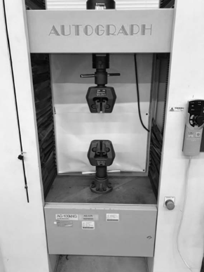
Figure 1. Autograph AG-100kNG.

In the experiments, the crosshead speed was 10[mm/min]. The Phantom high-speed camera was used to capture the bent panel just before buckling and just after buckling. The frame rate was 10000[frame/sec]. The length of folded area was 20.0[mm] at each ends, therefore the length of bending part was 260.0[mm]. By preserving the parallel and the same levels, we can compress them to observe the bending structure. We gradually compress the panel and then the panel broke suddenly. We refer the state critical state. At the state, we denote the height by $X_{\rm{c}}$, the width by $W_{\rm{c}}$ and the curvature by $k_{\rm{c}}$ as in Figure 3 (a). We call $k_{\rm{c}}$ critical curvature, $X_{\rm{c}}$ critical height and $W_{\rm{c}}$ critical width.. At the critical states, the shape of the elastic panels are displayed in Figure 2 (a), (b) and (c). The unit of scale in the background is given as 18.89[mm/unit]. The rupture needs the energy $\Delta E$ and the system lost the energy. After pieces of the broken elastic panel separate, the panel satisfies continuous condition at the bounce-back of the pieces and there appear a hinge which connects pieces. In other words, we find the $\Lambda$-elastica as in Figure 2 (d), (e) and (f). The hinge angle $\phi_{0}$ and the height $X_{\Lambda}$ is defined as in Figure 3 (b). As we are concerned with the transition from elastica to $\Lambda$-elastica at the critical state, the experimental results can be regarded as the transition.

In order to obtain these shapes, the notch was introduced at the surface of testing panel whose depth was 0.5[mm] and width was 1.0[mm] in the direction perpendicular to the longitudinal direction.

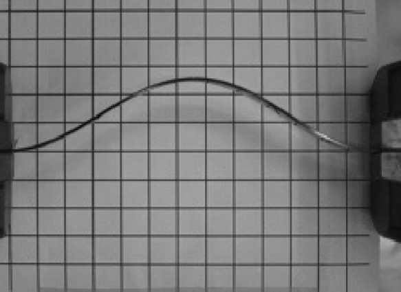
(a)

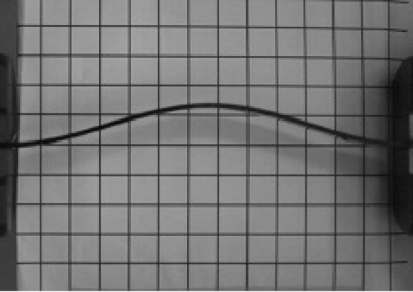
(b)

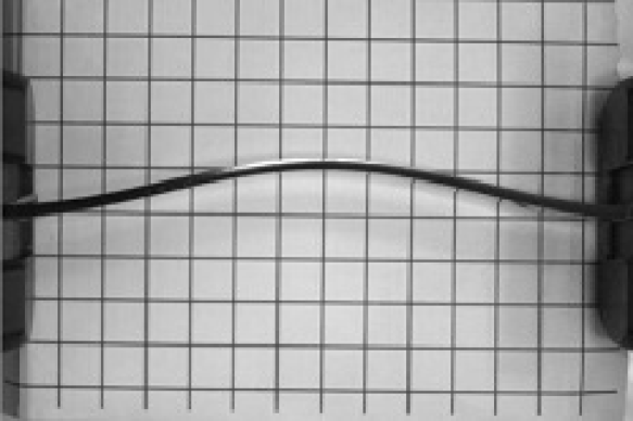
(c)

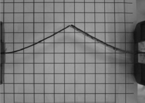
(d)

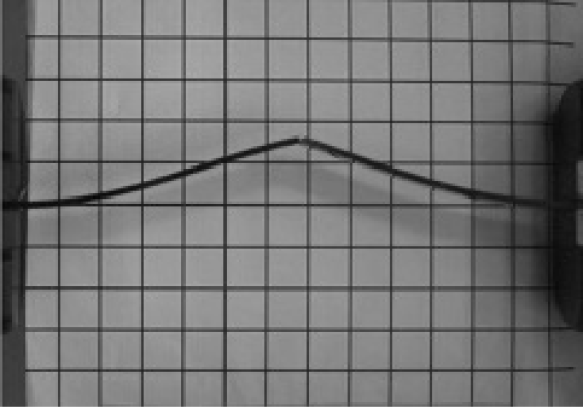
(e)

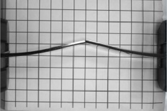
(f)

Figure 2. Press experiments of elastic beam: (a)-(c) are elastic panels with critical curvature whereas (d)-(f) are of $\Lambda_{\phi_{0}}$ shapes of elastic panels which appear at the bounce-back of the separated pieces of panels and they behave like continuum beams. The thickness $\delta$ of (a) and (d) are 2.0[mm], (b) and (e) correspond to 3.0[mm] and (c) and (f) to 5.0[mm].

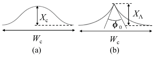
Figure 3. Geometrical Characteristics: $X_{\rm{c}}$, $W_{\rm{c}}$ and $\phi_{0}$

Dependence of $X_{\rm{c}}$, $W_{\rm{c}}$, $\phi_{0}$ and $X_{\Lambda}$ on the thickness $\delta$ is shown in Table 1. The thicker is, the lager the critical width $W_{\rm{c}}$ is. the smaller, the height $X_{\rm{c}}$ is and the larger the angle $\phi_{0}$ is. It should be noted that $X_{\Lambda}$ is nearly equal to $X_{\rm{c}}$.

Table 1: The thickness vs $X_{\rm{c}}$, $W_{\rm{c}}$, and $\phi_{0}$ in Figure 2 ($W_{0}=14.1$) $\delta$ $X_{\rm{c}}$ $W_{\rm{c}}$ $\phi_{0}$ $X_{\Lambda}$ 2.0 [mm] 49[mm] 234[mm] 0.66$\pi$ 51[mm] 3.0 [mm] 25[mm] 242[mm] 0.79$\pi$ 28[mm] 5.0 [mm] 21[mm] 250[mm] 0.86$\pi$ 23[mm]

It is hard to control the transition in this experiment but if there is a certain geometrical constraint so that it must be continuous even after it was broken, we may find $\Lambda$-elastica statically. By assuming the situation, we investigate this experimental result mathematically.

2.2. Thickness and elastic constant of the elastica

In order to show the relation between the thickness of elastic beam and the effective elastic constant, let us consider an embedding of the elastic beam with constant thickness $\delta$ in the complex plane ${\mathbb{C}}$. Assume that the center axis of the beam does not change its length. We estimate the stretching of the elastic beam. Let the curve be parallel to the center axis curve with the vertical distance $q$ from the center axis, which is parameterized by $s_{q}$ with the euclidean distance. The stretching of the curve is given by

$$ds_{q}=(1+k(s)q)ds,$$

where $s$ is the arclength of the center axis of the beam, $k(s)$ is the curvature whose inverse is the curvature radius $\rho(s)=1/k(s)$, and $q\in[-\delta/2,\delta/2]$. We assume the case $\delta/\rho=\delta\cdot k\ll 1$. It means that $e_{q}:=1+k(s)q=\displaystyle{\frac{\partial s_{q}}{\partial s}}$ is the ratio of the stretching length. The free energy density $\mathcal{F}dqds$ caused by bending is given by

$$\mathcal{F}dqds=\frac{1}{2}\kappa\left(\frac{\partial e_{q}}{\partial q}\right)^{2}(1+kq)dqds,$$

where $\kappa$ is the elastic constant. By integrating along the vertical direction, we have

(2.1) $$\begin{split}\left(\int_{-\delta/2}^{\delta/2}\mathcal{F}dq\right)ds&=\frac{1}{2}\delta\left(\kappa k^{2}+\frac{1}{2}\delta k^{3}\right)ds\\ &=\frac{1}{2}\delta\kappa k^{2}\left(1+o\left(\frac{\delta}{k}\right)\right)ds.\\ \end{split}$$

The factor $\kappa\delta$ is regarded as an effective elastic constant, which is proportional to the thickness $\delta$. (2.1) is known as the density of the Euler-Bernoulli energy functional.

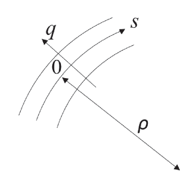
Figure 4. Modeling of elastic beam

Thus in the experiment results mentioned in Section 2.1, we have considered three cases which have different thickness.

3. Review of Euler’s Elastica

This section is devoted to review the elastica theory following [10].

3.1. Geometry of a Curve in Plane

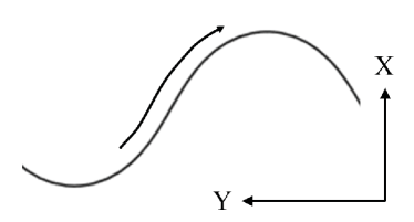
Figure 5. Elastic curve

Let $Z:(s_{1},s_{2})\to{\mathbb{C}}$ be an isometric analytic immersion with the arclength $s$ for $s_{1}<s_{2}$. In other words, we consider an analytic curve in a plane parameterized by the arc-length $s$; $Z(s)=X(s)+\sqrt{-1}Y(s)$, i.e., $|\partial_{s}Z|=1$, where $\partial_{s}:={\rm{d}}/{\rm{d}}s$. Its tangential vector is ${\bf t}:=\partial_{s}Z={\rm{e}}^{\sqrt{-1}\varphi}$ using the tangential angle $\varphi\in\{\varphi:(s_{1},s_{2})\to{\mathbb{R}}\ |\$ real analytic $\}$, whereas the normal vector is ${\bf n}=\sqrt{-1}{\bf t}$. We have the Frenet-Serret relation,

(3.1) $$\partial_{s}(\partial_{s}Z)={\sqrt{-1}}k\partial_{s}Z,$$

where $k:=\partial_{s}\varphi$ is the curvature (inverse of curvature radius $\rho(s)$) of the curve.

From (2.1), the Euler-Bernoulli energy functional of $Z$ is given by

(3.2) $${\mathcal{E}}[Z]=\frac{1}{2}\int_{(s_{1},s_{2})}k(s)^{2}\,{\rm{d}}s.$$

Let us consider its minimal point in the regular function space of $Z$,

$${\mathfrak{M}}_{(s_{1},s_{2})}:=\{Z:(s_{1},s_{2})\to{\mathbb{C}}\ |\ Z\mbox{ is an isometric analytic immersion}\},$$

which is called celebrated elastica [2, 4, 10, 13]. In order to obtain the minimal point of the energy functional, we consider an infinitesimal deformation

$$Z_{\varepsilon}(s_{\varepsilon})=Z(s)+{\bf n}\varepsilon(s),$$

which does not satisfy the isometric condition because

$$\partial_{s}Z_{\varepsilon}=(1-\varepsilon k(s)){\bf t}+(\partial_{s}\varepsilon)\varepsilon,$$

and

$$ds_{\varepsilon}^{2}=d\overline{Z_{\varepsilon}}dZ_{\varepsilon}=(1-2\varepsilon k)ds^{2}+o(\varepsilon^{2}).$$

The deformed curvature is given by

$$k_{\varepsilon}=k+(k^{2}+\partial_{s}^{2})\varepsilon+o(\varepsilon^{2}),$$

since

$$\frac{\partial^{2}}{\partial s_{\varepsilon}^{2}}Z_{\varepsilon}=(-(\partial_{s}\varepsilon)k){\bf t}+(k+(k^{2}+\partial_{s}^{2})\varepsilon){\bf n}+o(\varepsilon^{2}).$$

The deformed integrated of the Euler-Bernoulli functional is given by

$$k_{\varepsilon}^{2}ds_{\varepsilon}=(k^{2}+(k^{3}+2k\partial_{s}^{2})\varepsilon+o(\varepsilon^{2}))ds,$$

and thus we have the following proposition:

Proposition 3.1.

The curvature $k_{\rm{m}}$ of the minimizer $Z_{\rm{m}}$ of the Euler-Bernoulli energy functional (3.2), i.e., $\displaystyle{Z_{\rm{m}}|\ \min_{Z\in{\mathfrak{M}}_{(s_{1},s_{2})}}{\mathcal{E}}[Z]}$, satisfies

(3.3) $$ak_{\rm{m}}+\frac{1}{2}k_{\rm{m}}^{3}+\partial_{s}^{2}k_{\rm{m}}=0,$$

where $a$ is a constant real number for the Lagrange multiplier. We call $Z_{\rm{m}}$ elastica or elastic curve.

Proof.

The energy functional (3.2) is reduced to

(3.4) $$-\frac{\delta{{\mathcal{E}}+a\int_{(s_{1},s_{2})}ds_{\varepsilon}}}{\delta\varepsilon(s)}=k^{3}+2\partial_{s}^{2}k+ak=0$$

since we consider the isometric deformation. ∎

We note that there are uncountably infinite elasticas, $Z_{\rm{m}}$’s, depending on their ending conditions. From here we will consider only an element of the set ${\mathfrak{Z}}_{\rm{m}}$ of elasticas, which is simply denoted by $Z$ again in this section. The curvature $k_{\rm{m}}$ is also simply denoted by $k$.

We have the governing equation of elastica:

Proposition 3.2.

For a real constant $b$, the elastica obeys the equation

(3.5) $$(\partial_{s}k)^{2}+\frac{1}{4}k^{4}+ak^{2}+b=0.$$

Proof.

By multiplying (3.3) by $(\partial_{s}k)$ and integrating it, (3.3) becomes (3.5). Here $b$ is an integral constant. Due to the reality of $k$ and $s$, $b$ must be also real. ∎

3.2. Elastica in terms of elliptic functions

For later convenience, we introduce affine parameters,

$$x(s) := \frac{{\sqrt{-1}}}{4\alpha}\partial_{s}k+\frac{1}{8}k^{2}+\frac{1}{12}a,$$

$$y(s) := \frac{1}{2\alpha}\partial_{s}x=\frac{1}{2}\left[{\sqrt{-1}}\left(\frac{1}{8}k^{3}+\frac{1}{4}ak+\frac{{\sqrt{-1}}}{4\alpha}k\partial_{s}k\right)\right].$$

(3.5) means that we have an elliptic curve $C_{1}$ given by the affine equation,

(3.7) $$\begin{split}\frac{\hat{y}^{2}}{4}=y^{2}&=\left(x+\frac{1}{6}a\right)\left(x-\frac{1}{12}a-\frac{1}{4}\sqrt{b}\right)\left(x-\frac{1}{12}a+\frac{1}{4}\sqrt{b}\right)\\ &=(x-e_{1})(x-e_{2})(x-e_{3}),\\ \end{split}$$

where $e_{1}=-\frac{1}{6}a$, $e_{2}=\frac{1}{12}a+\frac{1}{4}\sqrt{b}$, and $e_{3}=\frac{1}{12}a-\frac{1}{4}\sqrt{b}$. For later convenience, we let $a^{2}-b=16$; $C_{1}=\{(x,y)\in{\mathbb{C}}^{2}\ |\$ (3.7) $\}\cup\{\infty\}$. They mean that $a=2(e_{2}+e_{3}-2e_{1})$, $b=-(e_{2}-e_{3})^{2}$. $(x,\hat{y})$ corresponds to the Weierstrass normal form [14].

For the curve $C_{1}$, the incomplete elliptic integral of the first kind is given by

(3.8) $$u=\int^{x}_{\infty}{\rm{d}}u,\qquad{\rm{d}}u=\frac{{\rm{d}}x}{2y}.$$

The complete elliptic integrals of the first kind as the double periodicity $(2\omega^{\prime},2\omega^{\prime\prime})$ are given by

$$\omega^{\prime}:=\int_{\infty}^{(e_{1},0)}{\rm{d}}u,\qquad\omega^{\prime\prime}:=\int_{\infty}^{(e_{3},0)}{\rm{d}}u,$$

whereas the complete elliptic integrals of the second kind are given by

(3.9) $$\eta^{\prime}=\int_{\infty}^{(e_{1},0)}{\rm{d}}r,\qquad\eta^{\prime\prime}=\int_{\infty}^{(e_{3},0)}{\rm{d}}r,$$

where

$${\rm{d}}r=\frac{x{\rm{d}}x}{2y}.$$

Using them, we define the Weierstrass sigma function $\sigma$ by

(3.10) $$\sigma(u)=\frac{2\omega^{\prime}}{2\pi{\sqrt{-1}}}\exp\left(\frac{\eta^{\prime}u^{2}}{2\omega^{\prime}}\right)\frac{\theta_{1}(u/\omega^{\prime})}{\theta_{1}^{\prime}(0)},$$

where $\tau=\omega^{\prime\prime}/\omega^{\prime}$ and

$$\theta_{1}(v)={\sqrt{-1}}\sum_{n=-\infty}^{\infty}\exp\left({\sqrt{-1}}\pi\left(\tau(n-1/2)^{2}+(2n-1)(v+1)\right)\right).$$

In terms of the sigma function, the Weierstrass $\zeta$-function and $\wp$ function are given by

(3.11) $$\zeta(u)=\frac{d}{du}\log\sigma(u),\qquad\wp(u)=-\frac{d^{2}}{du^{2}}\log\sigma(u).$$

We have an identity between $\zeta$-function and an integral of the second kind,

$$\zeta(u)=-\int^{(x,y)}_{\infty}{\rm{d}}r=-\int^{(x,y)}_{\infty}x{\rm{d}}u.$$

Then it is known that $(\wp(u),\partial_{u}\wp(u)/2)$ is identified with $(x,y)$ in $C_{1}$ by setting $u=\int^{(x,y)}_{\infty}{\rm{d}}u$; we identify both by $x(s)=\wp(\alpha s+u_{0})$ for a certain $u_{0}\in{\mathbb{C}}$.

3.3. Euler’s Elastica and $\zeta$ function

Following [10], we show the shape of elastica as a minimizer of ${\mathcal{E}}[Z]$ of ${\mathfrak{M}}_{(s_{1},s_{2})}$. Here we do not consider the boundary condition explicitly since $(s_{1},s_{2})$ has no boundary.

Theorem 3.3.

By choosing the origin of angle $\varphi$ and $u_{0}$,

(3.12) $$\partial_{s}Z(s)\equiv{\rm{e}}^{\sqrt{-1}\varphi}={\sqrt{-1}}(\wp(\alpha s+u_{0})-e_{1}),$$

(3.13) $$Z(s)=\frac{{\sqrt{-1}}}{\alpha}(-\zeta(\alpha s+u_{0})-e_{1}s)+Z_{0}.$$

Proof.

Noting $\displaystyle{{\sqrt{-1}}k=\frac{\alpha\wp_{u}(\alpha s+u_{0})}{\wp(\alpha s+u_{0})-e_{1}}}$ from (3.2), the tangential angle of the elastica is given by

(3.14) $$\varphi(s)=\frac{1}{\sqrt{-1}}\log\Bigr{(}\wp(\alpha s+u_{0})-e_{1}\Bigr{)}+\varphi_{0}.$$

It means that the tangential vector of elastica is represented by an elliptic function and we have an explicit formula of $Z$ using the elliptic $\zeta$ function. In other words, it is found that $k\equiv\partial_{s}\varphi$ of (3.2) satisfies (3.3) and (3.5) and vice versa. ∎

Remark 3.4.

We have the following relation:

(3.15) $$X(u)=X_{0}+\frac{\alpha}{4}k(s)$$

for an appropriate origin $X_{0}\in{\mathbb{R}}$.

In the computation of elastica, the condition that $\varphi$ and $s$ are real is necessary. We call the condition reality condition i.e., $|\partial_{s}Z|=1$ and $s$ is real.

Let us call the tangential period $\hat{\omega}$ of the (open) elastica that satisfies

$$\partial_{s}Z\left(s+\frac{\hat{\omega}}{\alpha}\right)=\partial_{s}Z(s).$$

Further we define an index of (open) elastica by

$$\mathrm{index}(\partial_{s}Z)=\frac{1}{2\pi{\sqrt{-1}}}\left(\log\partial_{s}Z\left(s+\frac{\hat{\omega}}{\alpha}\right)-\log\partial_{s}Z(s)\right).$$

Here we give a formula of the Euler-Bernoulli energy function;

Proposition 3.5.

$$\begin{split}\frac{1}{2}\int_{s_{1}}^{s_{2}}k(s)^{2}{\rm{d}}s=&\mathfrak{Re}\left(\frac{4}{\alpha}\left(\zeta(\alpha s_{1}+u_{0})-\zeta(\alpha s_{2}+u_{0})\right)-\frac{1}{3}a(s_{2}-s_{1})\right),\end{split}$$

where $\mathfrak{Re}(z)$ means the real part of $z$.

Proof.

$$\begin{split}\frac{1}{2}\int_{s_{1}}^{s_{2}}k^{2}{\rm{d}}s&=4\int_{s_{1}}^{s_{2}}\frac{1}{8}\wp(\alpha s+u_{0}){\rm{d}}s-4\int_{s_{1}}^{s_{2}}\frac{\sqrt{-1}}{4\alpha}(\partial_{s}k)-\frac{1}{3}a(s_{2}-s_{1})\\ =&\frac{4}{\alpha}\left(\zeta(\alpha s_{1}+u_{0})-\zeta(\alpha s_{2}+u_{0})\right)\\ &-\frac{\sqrt{-1}}{\alpha}(k(s_{2})-k(s_{1}))-\frac{1}{3}a(s_{2}-s_{1}).\\ \end{split}$$

Since $k$ is real, we have the expression. ∎

The number $\tau:=\omega^{\prime\prime}/\omega^{\prime}$ is a complex number called modulus, which determines the elliptic curve uniquely modulo trivial transformation, translation, dilatation and so on, and also determine the shape of elastica.

Due to the reality condition of the elastica, the moduli $\Xi$ of elastica is given by [12]

(3.16) $$\Xi:={\sqrt{-1}}\mathbb{R}_{>0}\cup\left(\frac{1}{2}+{\sqrt{-1}}\mathbb{R}_{>0}\right)\cup\{\infty\}\quad\mathrm{modulo}\quad\mathrm{PSL}(2,\mathbb{Z})$$

as a subspace of the moduli of elliptic curves, $\Xi\subset\mathbb{H}/\mathrm{PSL}(2,\mathbb{Z})$, where $\mathbb{H}$ is the upper half plane, i.e., $\mathbb{H}:=\{z\in\mathbb{C}\,;\Im z>0\}$.

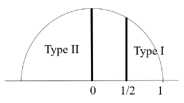
Figure 6. Moduli $\Xi$

This picture leads the classification of elastica as follows, without proof [10, 12];

(a)

(d)

(b)

(e)

(c)

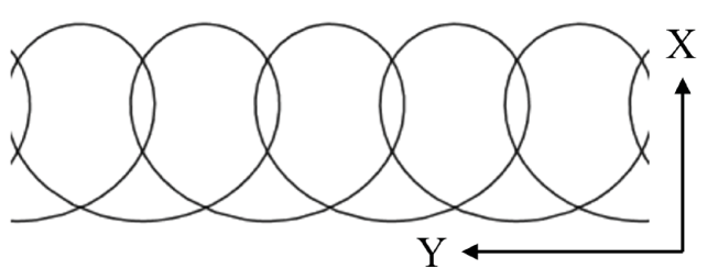
(f)

Figure 7. Types of Elastica: (a) shows type Ia, (b) is the rectangular elastica ($a=0$), (c) is type Ib, and (d)-(f) correspond to type II.

Proposition 3.6.

[10, 12]

1. Type Ia: for the case $-4\leq a\leq 0$, $\displaystyle{u_{0}=\left(\omega^{\prime\prime}-\frac{\omega^{\prime}}{2}\right)}$, $\hat{\omega}=2\omega^{\prime}\in{\mathbb{R}}$, $\displaystyle{\tau\in\left({\sqrt{-1}}\mathbb{R}_{>0}+\frac{1}{2}\right)}$ and $\mathrm{index}(\partial_{s}Z)$ is zero.

   We call $a=0$ case, the rectangular elastica, which corresponds to $\tau=\frac{1}{2}+\frac{1}{2}{\sqrt{-1}}$ and $1-\tau^{-1}={\sqrt{-1}}$.

2. Type Ib: for the case $0<a\leq 4$, $u_{0}=\displaystyle{-\frac{\omega^{\prime}}{2}}$, $\hat{\omega}=2\omega^{\prime}-4\omega^{\prime\prime}\in{\mathbb{R}}$, $\displaystyle{\tau\in\left({\sqrt{-1}}\mathbb{R}_{>0}+\frac{1}{2}\right)}$ and $\mathrm{index}(\partial_{s}Z)=0$.

3. Type II: for $4<a$, $u_{0}=\displaystyle{\frac{\omega^{\prime}}{2}}$, $\hat{\omega}=2\omega^{\prime\prime}\in{\mathbb{R}}$, $\tau\in{\sqrt{-1}}\mathbb{R}_{>0}$ and $\mathrm{index}(\partial_{s}Z)$ is equal to $\pm 1$.

Here $\mathbb{R}_{>0}$ is $\{x\in\mathbb{R}\,;x>0\}$.

4. Transition from elastica to $\Lambda_{\phi_{0}}$-elastica with hinge $\phi_{0}$.

In this section, we express the transition phenomenon from elastica to $\Lambda$-elastica. In order to express it,

1. we explicitly express the boundary condition in the theory of elastica in Section 3 (We introduce the function space ${\mathfrak{M}}_{[s_{1},s_{2}]}$ rather than ${\mathfrak{M}}_{(s_{1},s_{2})}$ and the boundary condition ${\mathfrak{B}}^{BT}_{W}$ with a parameter $W>0$.),

2. we introduce the novel function space ${\mathfrak{M}}^{s_{0},\phi_{0}}_{[s_{1},s_{2}]}$ in which the minimizer of the Euler-Bernoulli energy is $\Lambda$-elastica of hinge $\phi_{0}$,

3. we prepare the function space ${\mathfrak{M}}^{s_{0}}_{[s_{1},s_{2}]}$ which includes the ordinary elasticas, ${\mathfrak{M}}_{(s_{1},s_{2})}$, and $\Lambda$-elasticas ${\mathfrak{M}}^{s_{0},\phi_{0}}_{[s_{1},s_{2}]}$, and consider a disjoint orbit in ${\mathfrak{M}}^{s_{0}}_{[s_{1},s_{2}]}$ as the transition, and

4. using the symmetry, we set $s_{1}=-\frac{L}{2}$, $s_{2}=\frac{L}{2}$, $s_{0}=0$ and give the explicit results of the transition.

4.1. Preliminaries

From here, we discriminate the minimizer $Z_{\rm{m}}$ and the general immersion $Z$.

Let $\rho^{U}_{V}$ be the restriction of the domain of the function from $U$ to $V(\subset U)$. In order to impose the boundary condition, we consider

$$\begin{split}{\mathfrak{M}}_{[s_{1},s_{2}]}:=&\Bigr{\{}Z:[s_{1},s_{2}]\to{\mathbb{C}}\ |\ Z\mbox{ is differentiable at }s_{a}(a=1,2),\\ &\rho^{[s_{1},s_{2}]}_{(s_{1},s_{2})}Z\in{\mathfrak{M}}_{(s_{1},s_{2})}\Bigr{\}}.\end{split}$$

For a real parameter $\phi_{0}$ and $s_{0}\in(s_{1},s_{2})$, we introduce the function spaces,

$$\begin{split}{\mathfrak{M}}^{s_{0},\phi_{0}}_{(s_{1},s_{2})}:=&\Bigr{\{}Z:(s_{1},s_{2})\to{\mathbb{C}}\ \Bigr{|}\ \mbox{continues, }\phi_{0}=\displaystyle{\frac{1}{{\sqrt{-1}}}\log\frac{\partial_{s}Z(s_{0}+0)}{\partial_{s}Z(s_{0}-0)}},\\ &\rho^{(s_{1},s_{2})}_{(s_{1},s_{0})}Z\in{\mathfrak{M}}_{(s_{1},s_{0})},\rho^{(s_{1},s_{2})}_{(s_{0},s_{2})}Z\in{\mathfrak{M}}_{(s_{0},s_{2})}\Bigr{\}},\end{split}$$

$$\begin{split}{\mathfrak{M}}^{s_{0},\phi_{0}}_{[s_{1},s_{2}]}:=&\Bigr{\{}Z:[s_{1},s_{2}]\to{\mathbb{C}}\ |\ Z\mbox{ is differentiable at }s_{a}(a=1,2),\\ &\rho^{[s_{1},s_{2}]}_{(s_{1},s_{2})}Z\in{\mathfrak{M}}^{s_{0},\phi_{0}}_{(s_{1},s_{2})}\Bigr{\}},\end{split}$$

and

$${\mathfrak{M}}^{s_{0}}_{[s_{1},s_{2}]}:=\bigcup_{\phi_{0}\in[0,2\pi)}{\mathfrak{M}}^{s_{0},\phi_{0}}_{[s_{1},s_{2}]}.$$

We have a simple relation.

Lemma 4.1.

For given $s_{0}\in(s_{1},s_{2})$,

(4.1) $${\mathfrak{M}}^{s_{0},\phi_{0}}_{[s_{1},s_{2}]}\subset{\mathfrak{M}}^{s_{0}}_{[s_{1},s_{2}]},\quad{\mathfrak{M}}_{[s_{1},s_{2}]}\subset{\mathfrak{M}}^{s_{0}}_{[s_{1},s_{2}]}.$$

4.2. Elastica with boundary condition

In this subsection, we express the panel bending test by considering the boundary condition explicitly. For simplicity, we let $(s_{1},s_{2})=(-\frac{L}{2},\frac{L}{2})$ and introduce the boundary condition ${\mathfrak{B}}_{BT}$ which corresponds to the bending test in Section 2,

$$\begin{split}{\mathfrak{B}}^{BT}_{W}:=&\Bigr{\{}Z:\left[-\frac{L}{2},\frac{L}{2}\right]\to{\mathbb{C}}\ \Bigr{|}\ Z\mbox{ is differentiable at }\pm\frac{L}{2},\ \\ &Z\left(\pm\frac{L}{2}\right)=X_{0}+\frac{W}{2}{\sqrt{-1}},\ \partial_{s}Z\left(\pm\frac{L}{2}\right)={\sqrt{-1}}\Bigr{\}},\end{split}$$

where $W(>0)$ means the width of the ending of the elastica $Z$. The shape $Z_{\rm{m}}$ of the ordinary elastica in the compression testing apparatus is obtained as the minimizer

$$Z_{\rm{m}}^{W}|\min_{Z\in{\mathfrak{M}}_{[-\frac{L}{2},\frac{L}{2}]}\bigcap{\mathfrak{B}}^{BT}_{W}}{\mathcal{E}}[Z].$$

We obviously have the simple result;

Lemma 4.2.

$Z_{\rm{m}}^{L}([-\frac{L}{2},\frac{L}{2}])=\{X_{0}+s{\sqrt{-1}}\ |\ s\in[-\frac{L}{2},\frac{L}{2}]\}$.

It is noted that for $W\in(0,L]$, there are two points $Z_{\rm{m}}^{W}$, which are up-concave and down-concave. We are concerned only with a continuous deformation from the straight elastica $Z_{\rm{m}}^{L}$. We will choose the down-concave shapes. We consider one parameter deformation in ${\mathfrak{M}}_{[-\frac{L}{2},\frac{L}{2}]}$ for a deformation parameter $t\in I:=[0,1)$ with compression,

$$w(t)=(1-t)\cdot L.$$

Let us consider a continuous orbit in ${\mathfrak{M}}_{[-\frac{L}{2},\frac{L}{2}]}$,

$$Z_{\rm{co}}^{w}:I\to{\mathfrak{M}}^{0}_{[-\frac{L}{2},\frac{L}{2}]},\quad\left(t\mapsto Z_{\rm{co}}^{w}(t)=Z_{\rm{m}}^{w(t)}\in{\mathfrak{M}}_{[-\frac{L}{2},\frac{L}{2}]}\right).$$

Since $Z_{\rm{co}}^{w}$ is continuous and $Z_{\rm{co}}^{w}(0)=Z_{\rm{m}}^{L}$, $Z_{\rm{co}}^{w}$ is given by the following lemma.

Lemma 4.3.

For $a\in[-4,0]$, $Z_{\rm{co}}^{w}(t)(s)=\frac{{\sqrt{-1}}}{\alpha}(-\zeta(\alpha s+u_{0})-e_{1}s)+X_{0}$ where $\displaystyle{u_{0}=\left(\omega^{\prime\prime}-\frac{\omega^{\prime}}{2}\right)}$, $\hat{\omega}=2\omega^{\prime}\in{\mathbb{R}}$ and $\displaystyle{\alpha=\frac{\hat{\omega}}{L}}$ such that $w(t)=(Z_{\rm{co}}^{w}(t)(L/2)-Z_{\rm{co}}^{w}(t)(-L/2))/{\sqrt{-1}}$.

The case $a=-4$ corresponds to $Z_{\rm{m}}^{L}$ and $t=0$ whereas the case $a=0$ corresponds to the part of the rectangular elastica and $t=t_{R}:=0.8767723366$. $Z_{\rm{co}}^{w}$ expresses the deformation in the panel bending test and Lemma 4.3 shows the behavior of $Z_{\rm{co}}^{w}$ for $t\in[0,t_{R}]$.

For the elastica $Z_{\rm{co}}^{w}$, we denote its curvature by $k_{\rm{co}}^{w}$. Since the curvature $|k_{\rm{co}}^{w}(t)(s=0)|$ is the largest curvature in the elastic curve $Z_{\rm{m}}$, we fix the point $s_{0}$ by $s_{0}=0$ using the symmetry for the boundary condition.

4.3. $\Lambda_{\phi_{0}}$-elastica

With a certain boundary condition, the minimizer $Z_{\rm{m}}$ of the Euler-Bernoulli functional

$${\mathcal{E}}^{\Lambda_{\phi_{0}}}[Z]:={\mathcal{E}}[\rho^{(-\frac{L}{2},\frac{L}{2})}_{(-\frac{L}{2},0)}Z]+{\mathcal{E}}[\rho^{(-\frac{L}{2},\frac{L}{2})}_{(0,\frac{L}{2})}Z]$$

in ${\mathfrak{M}}^{s_{0},\phi_{0}}_{[s_{1},s_{2}]}$ is the $\Lambda_{\phi_{0}}$-elastica. We investigate it in this subsection.

Let us consider a disjoint orbit in ${\mathfrak{M}}^{0}_{[-\frac{L}{2},\frac{L}{2}]}$ as a transition from elastica to $\Lambda$-elastica. For a positive parameter $k_{\rm{c}}$, which we call critical curvature, we define the critical time $t_{\rm{c}}^{k_{\rm{c}}}$ by

$$t_{\rm{c}}^{k_{\rm{c}}}:=\sup_{t\in I}\left\{|k_{\rm{co}}^{w}(t)(0)|<k_{\rm{c}}\right\}.$$

We have the critical width

$$W_{\rm{c}}:=w(t_{\rm{c}}^{k_{\rm{c}}})=(1-t_{\rm{c}}^{k_{\rm{c}}})\cdot L.$$

Then we can express the transition from elastica to $\Lambda_{\phi_{0}}$-elastica as

$$Z^{k_{\rm{c}},\phi_{0}}_{{\rm{do}}}:I_{\rm{c}}\to{\mathfrak{M}}^{0}_{[-\frac{L}{2},\frac{L}{2}]},$$

where $I_{\rm{c}}:=[t_{\rm{c}}^{k_{\rm{c}}},1]$ and the disjoint orbit,

$$Z^{k_{\rm{c}},\phi_{0}}_{{\rm{do}}}(t):=\left\{\begin{array}[]{ll}Z_{\rm{co}}^{w}(t)&\mbox{for}t<t_{\rm{c}}^{k_{\rm{c}}}\\ Z_{\rm{m}}|\displaystyle{\min_{Z\in{\mathfrak{M}}^{0,\phi_{0}}_{[s_{1},s_{2}]}\bigcap{\mathfrak{B}}^{BT}_{w(t)}}{\mathcal{E}}^{\Lambda_{\phi_{0}}}[Z]},&\mbox{for }t=t_{\rm{c}}^{k_{\rm{c}}}\end{array}\right..$$

The following proposition is obvious:

Proposition 4.4.

The minimizer $Z_{\rm{m}}$ of ${\mathcal{E}}^{\Lambda_{\phi_{0}}}[Z]$ in ${\mathfrak{M}}^{s_{0},\phi_{0}}_{[s_{1},s_{2}]}$ consists of the parts of elastica.

Remark 4.5.

The $\Lambda_{\phi_{0}}$-elastica can be regarded as a curve of picewised elastica. Thus we can apply the Weierstrass-Erdmann corner conditions to this system directly [5], though we employ another approach.

Following Proposition 4.4, we numerically compute $\Lambda_{\phi_{0}}$-elastica. For $\phi_{0}=\pi/4$, the numerical computations shows a disjoint orbit $Z^{k_{\rm{c}},\phi_{0}}_{0}(t)$ illustrated in Figure 8. We set $L=1$.

In the computation, we used the Maple 2019. We assume that $\Lambda^{\phi_{0}}$-elastica consisting of type II elastica in Proposition 3.6 is the minimizer of ${\mathcal{E}}^{\Lambda_{\phi_{0}}}[Z]$. In other words, we searched the minimal point only in type II elastica for $\Lambda^{\phi_{0}}$-elastica, even though there are other local minimal points in the function space because the shape which satisfy the boundary condition and is given by type II elastica obviously seems to have smaller curvature than the shapes consisting of other type elastica; we do not argue the other possibilities in this paper.

We fix the parameter $a\in[4,\infty)$ in type II elastica. From Proposition 3.6, we find $\alpha s_{1}$ and $\alpha s_{2}$ so that these points correspond to the minimal $X_{\rm{m}}$, e.g., in Figure 7 (f), which satisfies the boundary condition $\partial_{s}Z_{\rm{m}}(s_{i})={\sqrt{-1}}$, $(i=1,2)$ using (3.12). We numerically found $\alpha s_{0}$ for the transcendental equation,

$$\log(\partial_{s}Z_{\rm{m}}(s_{0}))=\phi_{0}{\sqrt{-1}}$$

using (3.14). It determines $\alpha$ because of $\alpha(s_{1}-s_{0})=L/2$ and then we have the width $W_{II}$ as a function of $a$. Thus for a given width $W_{\rm{c}}$, using the bisection method, we found $a$ which reproduces $W_{\rm{c}}$ up to a certain error.

The shape of $\Lambda_{\phi_{0}}$-elastica and the transition is given in Figure 8 (c)-(a). We define the energy gap by

(4.2) $$\Delta{\mathcal{E}}^{\Lambda_{\phi_{0}}}:=\lim_{t\to t_{\rm{c}}-0}{\mathcal{E}}[Z^{k_{\rm{c}},\phi_{0}}_{0}(t)]-{\mathcal{E}}^{\Lambda_{\phi_{0}}}[Z^{k_{\rm{c}},\phi_{0}}_{0}(t_{\rm{c}}^{k_{\rm{c}}})].$$

In the case of Figure 8, $\Delta{\mathcal{E}}^{\Lambda_{\phi_{0}}}$ is positive, as in Figure 8 (f). It means that by the transition, total energy decreases; the $\Lambda$-elastica is stabler than the ordinary elastica.

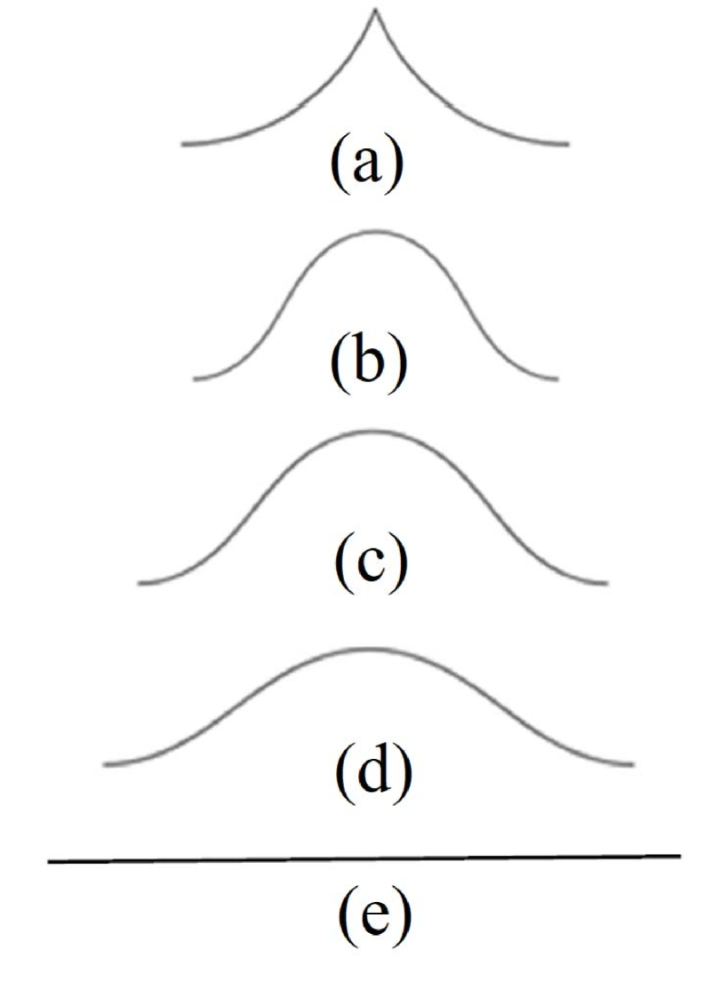
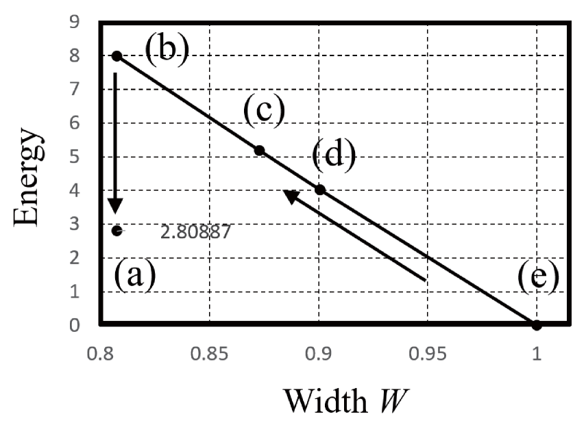
(f)

Figure 8. A transition: (a)-(e) shows the orbit from elastica to $\Lambda_{\phi_{0}}$ elastica; from (e) to (a), whereas for the orbit, the total energy is illustrated in (f). The width of (b) is the same as that of (a), which corresponds to the critical width. In the computation, we let $L=1$ and $\kappa=1$.

Under this boundary condition, (3.13) and Proposition 3.5 mean that the relation between the width $W$ and the energy ${\mathcal{E}}[Z_{\rm{m}}^{W}]$ is given as a linear equation,

(4.3) $${\mathcal{E}}[Z_{\rm{m}}^{W}]=E_{0}(L-W)$$

because both are written by the Weierstrass’ zeta functions.

It is obvious to have the positivity of the energy gap from the fact (4.1):

Proposition 4.6.

$$\Delta{\mathcal{E}}^{\Lambda_{\phi_{0}}}:=\sup_{\phi_{0}\in[0,\pi)}\Delta{\mathcal{E}}^{\Lambda_{\phi_{0}}}$$

is non-negative.

However for given $\phi_{0}$ and $W_{\rm{c}}$, the positiveness of $\Delta{\mathcal{E}}^{\Lambda_{\phi_{0}}}$ is not guaranteed but there exists $\phi_{0}$ whose $\Delta{\mathcal{E}}^{\Lambda_{\phi_{0}}}$ is non-negative since the case $\phi_{0}=\pi$ corresponds to ordinary elastica. It might be expected that $\phi_{0}$ should be determined as a minimal point of the energy $\Delta{\mathcal{E}}^{\Lambda_{\phi_{0}}}$ in the parameter space $\phi_{0}\in[0,\pi]$.

We computed the cases with several conditions of $W_{\rm{c}}$ and $\phi_{0}=0,\pi/4,\pi/2$ numerically and draw up lists of them as in Figures 9 and 10, and Table 2-6. Figure 10 shows the table of the elastica and $\Lambda_{\phi_{0}}$-elastica. The blank in Figures 10 and Table 2-6 means that we cannot find the $\Lambda_{\phi_{0}}$-elastica; more precisely we can find shape which satisfies the boundary conditions at $s_{1}$, $s_{0}$ and $s_{2}$ but since it has the much higher energy, we do not employ it as $\Lambda_{\phi_{0}}$-elastica in this paper. In this computation, we also used the algorithm as mentioned above. Table 2 shows the computed width of each shape by the bisection method. Table 3 shows the height $X_{\rm{c}}$ and $X_{\Lambda}$ for every width $W$. Table 4 shows the elastica parameter $a$ of each shape and Table 5 shows the imaginary part $\tau_{i}$ of the moduli parameter $\tau$ of elliptic function, i.e., $\tau_{i}$ of $\tau=1/2+\tau_{i}{\sqrt{-1}}$ for the elastica and $\tau=\tau_{i}{\sqrt{-1}}$ for the $\Lambda_{\phi_{0}}$-elastica. Table 6 gives each energy ${\mathcal{E}}[Z]$ and ${\mathcal{E}}^{\Lambda_{\phi_{0}}}[Z]$. We display the results in Figure 9.

Table 2: Width $W_{\rm{c}}$ computed by means of the bisection method $\phi_{0}$ $W_{5}$ $W_{4}$ $W_{3}$ $W_{2}$ $W_{1}$ $\pi/2$ 0.872 0.900 $\pi/4$ 0.807 0.873 0.901 $0$ 0.648 0.742 0.808 0.872 0.901 elastica 0.645 0.742 0,808 0.873 0.901

Table 3: Height $X_{\rm{c}}$ and $X_{\Lambda}$ $\phi_{0}$ $W_{5}$ $W_{4}$ $W_{3}$ $W_{2}$ $W_{1}$ $\pi/2$ 0.186 0.186 $\pi/4$ 0.245 0.186 0.154 $0$ 0.313 0.261 0.212 0.151 0.119 elastica 0.334 0.297 0,262 0.218 0.194

Table 4:Elastica parameter $a$ in the computations $\phi_{0}$ $W_{5}$ $W_{4}$ $W_{3}$ $W_{2}$ $W_{1}$ $\pi/2$ 45.0 10000.0 $\pi/4$ 6 4.08 4.0148 $0$ 20.0 4.45 4.06 4.0023 4.000167 elastica -1.3 -2 -2.5 -3 -3.215

Table 5:Imaginary part $\tau_{i}$ of the moduli parameter $\tau$ $\phi_{0}$ $W_{5}$ $W_{4}$ $W_{3}$ $W_{2}$ $W_{1}$ $\pi/2$ 0.3492 0.1586 $\pi/4$ 0.6080 1.1749 1.4429 $0$ 0.4272 0.9036 1.2205 1.7390 2.1560 elastica 0.5826 0.6396 0.6914 0.7617 0.8902

Table 6: Energy ${\mathcal{E}}[Z]$ and ${\mathcal{E}}^{\Lambda_{\phi_{0}}}[Z]$ $\phi_{0}$ $W_{5}$ $W_{4}$ $W_{3}$ $W_{2}$ $W_{1}$ $\pi/2$ 1.23 1.23 $\pi/4$ 2.81 3.67 4.60 $0$ 4.94 5.64 7.22 10.76 13.81 elastica 15.45 10.96 7.99 5.18 4.03

Remark 4.7.

For given $\phi_{0}$ and $W_{\rm{c}}$, the positiveness of $\Delta{\mathcal{E}}^{\Lambda_{\phi_{0}}}$ is not guaranteed as in Figure 9. Figure 9 shows that in many cases, $\Delta{\mathcal{E}}^{\Lambda_{\phi_{0}}}$ is positive whereas there exist the case in which $\Delta{\mathcal{E}}^{\Lambda_{\phi_{0}}}$ is negative.

We assume that for given $k_{\rm{c}}$ and $\phi_{0}$, $Z^{k_{\rm{c}},\phi_{0}}_{0}(t_{\rm{c}}^{k_{\rm{c}}})$ consists of elastica of type II, though we did not compare the other local minimum of the elastica which has the boundary condition. Then the transition from elastica to $\Lambda$-elastica is given by a map in the moduli space of the elastica as in Table 5. It is quite interesting from the viewpoint of the study on the moduli of elastica.

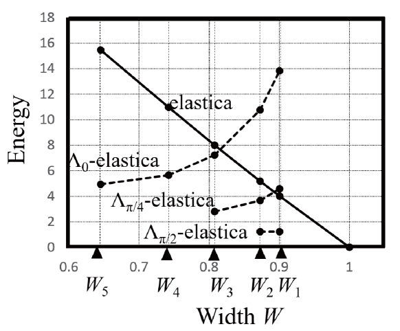
Figure 9. $\Lambda_{\phi_{0}}$-elastica and energy in Table 2-6

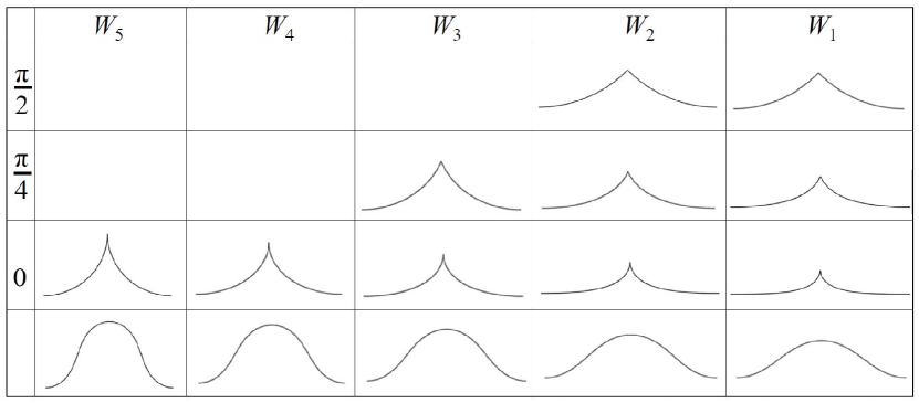
Figure 10. Elastica and $\Lambda_{\phi_{0}}$-elastica in Table 2-6

5. Discussion

In this paper, we investigated the $\Lambda$-elastica. We explicitly show the shape of $\Lambda_{\phi_{0}}$-elastica in terms of Weierstrass elliptic $\zeta$-functions, and numerically showed it in Figures 8 and 10. By estimating their energy, we also considered the transition from elastica to $\Lambda$-elastica and stability from the viewpoint of energetic study. The energy gap $\Delta{\mathcal{E}}^{\Lambda_{\phi_{0}}}$ in (4.2) are numerically computed and illustrated in Figure 9 and Table 6.

When we compare the computational results and experimental results in Section 2, the effective elastic constant is crucial, which is proportional to the thickness $\delta$, whereas we used the normalized elastic constant, $\kappa=1$, in the computations. The thickness $\delta$ of the elastic panel has the energy $\delta\cdot\Delta{\mathcal{E}}^{\Lambda_{\phi_{0}}}$ and, for examples, the values in the graph of Figure 9 should be multiplied by its thickness $\delta$. In order to consider the effect of $\delta$, Table 1 reads the following table, Table 7.

Table 7: The thickness vs $X_{\rm{c}}$, $W_{\rm{c}}$, $\phi_{0}$ and $X_{\Lambda}$ in Figure 2 $\delta$ $X_{\rm{c}}$ $\delta\cdot X_{\rm{c}}$ $W_{\rm{c}}$ $\delta(L-W_{\rm{c}})$ $\phi_{0}$ $X_{\Lambda}$ $\delta\cdot X_{\Lambda}$ 2.0 [mm] 49[mm] 98[mm²] 234[mm] 51[mm²] 0.66$\pi$ 51[mm] 102[mm²] 3.0 [mm] 25[mm] 74[mm²] 242[mm] 52[mm²] 0.79$\pi$ 28[mm] 85[mm²] 5.0 [mm] 21[mm] 104[mm²] 250[mm] 49[mm²] 0.86$\pi$ 23[mm] 113[mm²]

From (4.3), $E(\delta):=\delta\cdot(L-W_{\rm{c}})$’s correspond to the elastic energy at the critical state, which are similar values, though the width in photographs in Figure 2 is not easy to be determined and must have some errors. On the other hand, from (3.15), it is expected that the force $\delta\cdot k_{\rm{c}}$ is proportional to $\delta\cdot X_{\rm{c}}$ (up to $\alpha$-dependence) depend on the material properties though we made the notch in each panel, Table 7 gives the natural results, in which $\delta\cdot X_{\rm{c}}$’s are similar values. The height of $\Lambda$-elastica $X_{\Lambda}$ is nearly equal to $X_{\rm{c}}$ for every $\delta$ and thus $\delta\cdot X_{\Lambda}$’s are similar values though we cannot compare $\delta\cdot X_{\rm{c}}$ and $\delta\cdot X_{\Lambda}$ from mechanical viewpoints because $\alpha$’s in (3.15) of both elasitca and $\Lambda$-elastica are irrelevant.

In the experiment, it is expected that $\delta\cdot\Delta{\mathcal{E}}^{\Lambda_{\phi_{0}}}$ corresponds to the energy of rupture. After the panel lost the energy of rupture, $\phi_{0}$ of $\Lambda_{\phi_{0}}$-elastica is determined by energy conservation law.

Thus we note that Figure 9 and Figure 10 are consistent with the experimental results; the larger $W_{\rm{c}}$ is, the larger $\phi_{0}$ is. Our numerical computations also show that the lager $W_{\rm{c}}$ is, the lager $\phi_{0}$ is because the energy gap needs positive.

It means that we provide a novel investigation of rupture phenomena for the beam bending test. Further the shape of $\Lambda$-elastica is very interesting since the shape of $\Lambda$-elastica appears in [11] and in [3]. As mentioned above, we described the transition from elastica to $\Lambda$-elastica in the beam bending experiment and $\Lambda$-elastica mathematically. We hope that our investigation should have some effects on these studies.

Shigeki Matsutani:
Faculty of Electrical, Information and Communication Engineering,
Kanazawa University
Kakuma Kanazawa, 920-1192, JAPAN
e-mail: s-matsutani@se.kanazawa-u.ac.jp

Hiroshi Nishiguchi:
National Institute of Technology, Sasebo College,
1-1 Okishin-machi, Sasebo, Nagasaki, 857-1193, JAPAN

Kenji Higashida:
National Institute of Technology, Sasebo College,
1-1 Okishin-machi, Sasebo, Nagasaki, 857-1193, JAPAN

Akihiro Nakatani:
Department of Adaptive Machine Systems,
Graduate School of Engineering, Osaka University, 2-1 Yamadaoka, Suita, Osaka 565-0871, JAPAN

Hiroyasu Hamada:
National Institute of Technology, Sasebo College,
1-1 Okishin-machi, Sasebo, Nagasaki, 857-1193, JAPAN

References

- [1] Bigoni, D, Nonlinear Solid Mechanics: Bifurcation Theory and Material Instability, Cambridge Univ. Press, 2014.
- [2] Bryant R. and Griffiths P., Reduction for Constrained Variational Problems and , Amer. J. Math. 108 (1986) 525-570.
- [3] Dharmadasa Y, Mallikarachchi H.M.Y.C., and López Jiménez F., , Characterizing the Mechanics of Fold-lines in Thin Kapton Membranes, AIAA SciTech Forum , 8-12 January 2018, Kissimmee, Florida, 10.2514/6.2018-0450.
- [4] Euler L., Methodus Inveniendi Lineas Curvas Maximi Minimive Proprietate Gaudentes, 1744, Leonhardi Euleri Opera Omnia Ser. I vol. 14.
- [5] Gelfand, I. M. and Fomin, S. V., Calculus of Variations, Dover Publications, 2012.
- [6] Goldstein R. and Petrich D., The Korteweg-de Vries Hierarchy as Dynamics of Closed Curves in the Plane, Phys. Rev. Lett. 67 (1991) 3203-3206.
- [7] Hagihara K., Yokotani N. and Umakoshi Y., Plastic deformation behavior of Mg12YZn with 18R long-period stacking ordered structure, Intermetallics 18 (2010) 267-276.
- [8] Hess J. B. and Barrett C. S., Trans Am Inst Min Met Eng. 185 (1949) 599-606.
- [9] Mladenov, I. M., Hadzhilazova, M., The Many Faces of Elastica (Forum for Interdisciplinary Mathematics), Springer, 2017.
- [10] Matsutani S., Euler’s elastica and its beyond, J. Symm. Geom. Phys. 17 (2013) 45-86.
- [11] Morigaki Y., Wada H. and Tanaka Y., Stretching an Elastic Loop: Crease, Helicoid, and Pop Out, Phys. Rev. Lett. 117 (2016) 198003.
- [12] Mumford D., Elastica and Computer Vision, in Algebraic Geometry and its Applications, ed. by C. Bajaj, Springer-Verlag Berlin 1993 507-518.
- [13] Truesdell C., The Influence of Elasticity on Analysis: The Classic Heritage, Bull. Amer. Math. Soc. 9 (1983) 293-310.
- [14] Whittaker E. and Watson G., A Course of Modern Analysis, 4th ed. Cambridge Univ. Press, Cambridge, 1927.