Chemical evolution along the circumnuclear ring of M83

Abstract

We report an astrochemical study on the evolution of interstellar molecular clouds and consequent star formation in the center of the barred spiral galaxy M83. We used the Atacama Large Millimeter/submillimeter Array (ALMA) to image molecular species indicative of shocks (SiO, CH₃OH), dense cores (N₂H⁺), and photodissociation regions (CN and CCH), as well as a radio recombination line (H41$\alpha$) tracing active star-forming regions. M83 has a circumnuclear gas ring that is joined at two areas by gas streams from the leading-edge gas lanes on the bar. We found elevated abundances of the shock and dense-core tracers in one of the orbit-intersecting areas, and found peaks of CN and H41$\alpha$ downstream. At the other orbit-intersection area, we found similar enhancement of the shock tracers, but less variation of other tracers, and no sign of active star formation in the stream. We propose that the observed chemical variation or lack of it is due to the presence or absence of collision-induced evolution of molecular clouds and induced star formation. This work presents the most clear case of the chemical evolution in the circumnuclear rings of barred galaxies, thanks to the ALMA resolution and sensitivity.

1 Introduction

1.1 Astrochemistry and properties of the interstellar medium

The chemical composition of a molecular cloud is a sensitive probe of its physical conditions. The abundances of various molecules in Galactic star-forming cores are known to evolve with the stages of star formation (Caselli & Ceccarelli, 2012). The chemistry of a molecular cloud also reflects its environments such as the strong UV radiation (e.g., Hollenbach & Tielens, 1997) or shocks (e.g., Hollenbach & McKee, 1979).

The diagnostic power of astrochemistry can also be applied to a collection of molecular clouds in external galaxies. For example, galaxies with extreme starburst or nuclear activities are expected to have chemical compositions distinct from that in our Galaxy. To study the characteristic chemical compositions in such galaxies, spectral scan observations have been conducted in various types of galaxies both with single-dish telescopes and interferometers (Meier & Turner, 2005; Martín et al., 2006b; Aladro et al., 2015; Takano et al., 2019). While single-dish studies have been useful identifying molecular species whose galaxy-wide abundances change according to the types of galaxies, spatially-resolved interferometric observations should better highlight the chemistry in regions with most extreme physical conditions. Thanks to the high sensitivity and angular resolution of Atacama Large Millimeter/sub-millimeter Array (ALMA), such astrochemical studies have become practical for various types of galaxies. In particular, relationship between the galactic structures and the chemistry within galactic center regions has been revealed in multi-species astrochemical observations using ALMA (e.g., Takano et al., 2014; Nakajima et al., 2015; Martín et al., 2015; Meier et al., 2015).

With spatially-resolved astrochemistry in an external galaxy, one can effectively study the time evolution of the chemical and physical properties of the interstellar medium (ISM) in response to large-scale gas dynamics. This is because a spatial variation of gas properties in a gas flow can be interpreted as a time evolution of the ISM in the flow.

1.2 Galactic gas dynamics and ISM evolution

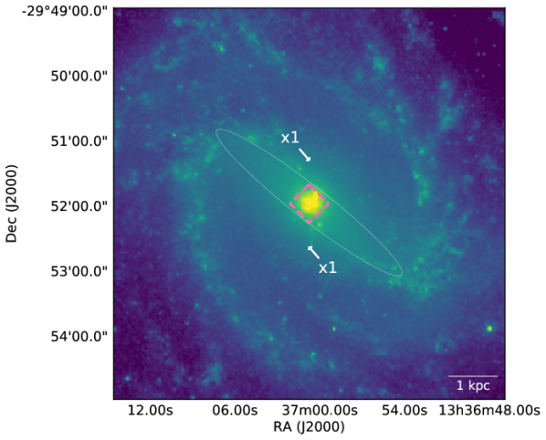
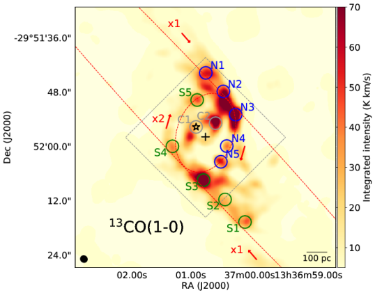
Figure 1: (Left) Spitzer IRAC 3.6 $\mu m$ image of M83 from Dale et al. (2009). The target area of our observations are indicated as a pink dashed rectangule. An example of $x_{1}$ (bar) orbits is shown as a white ellipse. (Right) The velocity-integrated intensity map of ¹³CO($1-0$). This is to show the structure of circumnuclear ring and analyzed positions. The target area of our observations is indicated as a grey dashed rectangle. Positions analyzed in this paper are indicated as blue (N1-5), green (S1-5), and grey (C1-2) circles. The star indicates the position of nucleus (Houghton & Thatte, 2008), and the plus sign shows the location of the center of symmetry. The synthesized beam is shown as a black ellipse on the lower left corner. Examples of $x_{1}$ and $x_{2}$ (circumnuclear ring) orbits are shown with red dashed ellipses. There is the same map in Appendix A with contours. The “typical” value of rms is $\sigma_{\rm N1}=0.57$ K km s^-1 in this map.

A galactic center often hosts a significant fraction of star formation in the galaxy, and the gas supply necessary for the star formation is closely related to galactic gas dynamics. In a barred spiral galaxy, the interstellar gas can efficiently flow into the central region because of the shocks on the bar and gravitational torque on the gas in the bar (Sorensen et al., 1976; Matsuda & Nelson, 1977; Combes & Gerin, 1985). Consequently, barred galaxies tend to have higher concentration of molecular gas to their centers (Sakamoto et al., 1999), and higher star formation activities at the galactic centers (Ho et al., 1997). The outline of the relevant gas dynamics is illustrated in Figure 1. The gas in the bar is, outside the central region, on the so-called $x_{1}$ orbits elongated along the bar (Figure 1 left). The leading-edge gas lanes frequently seen in galactic bars are on these orbits. Near the center of the bar, there is often a ring-like structure on the so-called $x_{2}$ orbits. This structure is sometimes referred to as the (circum-)nuclear ring (Comerón et al., 2010, see Figure 1 right). Simulations have shown that a circumnuclear ring connected to the leading-edge lanes on the bar naturally result from the non-axisymmetric gravitational potential (Athanassoula, 1992). When the gas flows from the bar through the leading-edge lanes into the circumnuclear ring, collisions between molecular clouds on the $x_{1}$ and $x_{2}$ orbits should frequently occur at the accumulation points near orbit intersections. These collisions can unleash star formation events.

Molecular cloud collisions have been proposed as a possible mechanism to trigger star formation (Elmegreen, 1998). There are many pieces of observational evidence pointing to cloud collisions promoting formation of massive stars in the Galactic spiral-arm regions (e.g., Furukawa et al., 2009; Torii et al., 2011; Fukui et al., 2014; Torii et al., 2015; Fukui et al., 2018) and the Galactic Center clouds (Tsuboi et al., 2015). Magneto-hydrodynamic simulations have also confirmed that collisions can trigger massive star formation (Inoue et al., 2018). While observations of collision-induced star formation in the Galaxy provide detailed views of individual collision sites, they provide the information only at the current state of those objects. In contrast, nearby galaxies, especially face-on galaxies, provide an ideal setting to study time evolution of the ISM through cloud collisions as spatial variation along the gas orbits.

Collision-induced star formation at the orbit intersection can appear in the form of gradients in stellar ages. Böker et al. (2008) proposed that two possible modes of star formation in circumuclear rings can cause different distributions of stellar ages. One mode is caused by the gravitational collapse of molecular clouds after certain densities are reached in circumnuclear rings (Elmegreen, 1994). In this scenario, there is no dependence of star formation on the azimuthal angle on the circumnuclear ring, and stellar clusters with a wide range of ages should be randomly located. Another scenario is that the star formation is triggered by the collision between the gas on the bar orbit and the gas on the circumnuclear ring. In this mode, young star clusters should preferentially exist at the orbit intersections, and there should an stellar age gradient along the stream. In the sample of Böker et al. (2008), three out of five galaxies showed such an age gradient. In a larger sample, Mazzuca et al. (2008) found that such an age gradient is present in about a half of their sample of 20 barred galaxies with circumnuclear rings.

The interaction of the gas on the circumnuclear ring and on the bar is also expected to alter the properties of the ISM. Kohno et al. (1999) found that the HCN/CO ratio, commonly used as a proxy of the fraction of dense molecular gas, is higher slightly downstream from the orbit intersection in NGC 6951. Even further downstream, there is an H$\alpha$ peak indicating active star formation. Although the higher-resolution follow up study by Krips et al. (2007) showed weaker enhancement of HCN/CO than in Kohno et al. (1999), there still was the general trend of higher HCN/CO downstream although Krips et al. (2007) interpreted those enhancements to be random and unrelated to the orbits. Such a change in the ISM properties was found also in NGC 7552 with higher HCN/CO observed at the orbit intersections (Pan et al., 2013). On the other hand, the excitation conditions of the molecular gas are not observed to change at the orbit intersection in the case of NGC 1097 (Hsieh et al., 2011).

1.3 Previous astrochemical studies in the circumnuclear rings and this work

Since the chemical composition is sensitive to various ISM conditions, the astrochemical approach using many species can better probe the ISM evolution in the circumnuclear rings of galaxies compared to the approach using a small number of line ratios. Such an astrochemical study was first conducted by Meier & Turner (2005) in the center of the barred spiral galaxy IC 342. They observed eight molecules (C₂H, C³⁴S, N₂H⁺, CH₃OH, HNCO, HNC, HC₃N, and SO) in IC 342 using the Owens Valley Millimeter Array, and showed that various molecular species peak at different locations. They proposed that shock tracers, CH₃OH and HNCO, are enhanced at locations of shocks at the intersections of the circumnuclear ring and the bar leading-edge gas lanes, that N₂H⁺ traces the overall dense gas, and that a photodissociation region (PDR) tracer C₂H is enhanced at locations with high star formation rate at the center of the nuclear ring.

It is worthwhile to follow up the astrochemical variation along the circumnuclear ring with the much improved sensitivity and resolution of ALMA. To study the variation of molecular composition caused by the galactic structure and dynamics, M83 provides an excellent laboratory due to its proximity ($d\sim 4.5\,$Mpc ($1^{\prime\prime}=22\,$pc); Thim et al., 2003), accessibility to ALMA, its face-on configuration, and presence of a circumnuclear ring. It is a barred spiral galaxy with the morphological type of SAB(s)c (de Vaucouleurs et al., 1991). The galactic bar has the length of 200^′′ (4.4 kpc) on the sky as seen from the $3.6\,\mu$m image in Figure 1 (left), and the structures of spiral arms are also clearly seen there. Such structures have also been seen with CO($J=1-0$) observations (Lundgren et al., 2004b; Hirota et al., 2014) to trace molecular gas. At the center, there is a circumnuclear ring with the size of 12-16^′′ on the sky (260-350 pc) as shown in Figure 1 (right).

In this paper, we report the first spatially resolved, interferometric astrochemical study in the central region of M83 using ALMA observations. Using astrochemical tracers, we study changes in the ISM properties most likely due to collisions of molecular clouds at the orbit intersections of the bar leading edge and the circumnuclear ring. The observed changes suggest eventual collision-induced star formation. The organization of this paper goes as follows. In Section 2, we summarize our observations and analysis method. Next, our results are summarized in Section 3 to show the chemical variation along the circumnuclear ring. We propose an explanation for such chemical variation as well as other possible scenarios in Section 4. Finally, a summary is given in Section 5.

2 Observations and data reduction

Our observations covering six tunings were conducted during ALMA cycle 4 using both the 12-m array and the 7-m array (project code: 2016.1.00164.S; PI: Harada). We targeted the entire circumnuclear ring, and we mosaicked the area of $25\arcsec\times 25\arcsec$ (see Figure 1 left) for Band 6 and Band 7, whose primary beam sizes are smaller than our targeted area. We supplemented our data with ALMA archival data 2012.1.00762.S (PI: Hirota) for CN($N=1-0$) and 2015.1.01177.S (PI: Longmore) for CCH($N=1-0$) and SiO($2-1$) lines. The former obervations included the 7-m array while the latter only had the 12-m array. The observational parameters are summarized in Table 1. The data cubes from 2012.1.00762.S were created in the data reduction procedure described in Hirota et al. (2018), and smoothed to the velocity resolution of 10.6 km s^-1. The data of 2016.1.00164.S and 2015.1.01177.S were reduced with the following processes. Measurement sets were calibrated with the CASA pipeline versions 4.6, 4.7 or 4.7.2. Imaging was conducted with CASA version 5.4 using the task tclean, and the imaging parameters used for individual lines are listed in Table 2. All the cubes were smoothed to 10 km s^-1 resolution except for CN(1-0) lines smoothed to 10.6 km s^-1. Missing flux was assessed for the lines in Band 3 by comparing our line fluxes with those from the IRAM 30-meter line survey in the 3-mm band by Aladro et al. (2015). The flux recovery rates are shown in Table 2. Most lines have the flux recovery rates higher than 70 % except for CH₃CCH (63 %) and HNCO (65 %). The missing flux is likely insignificant in our analysis because we analyze molecular emission at relatively compact peaks. The maximum recoverable scale is at least 16^′′ in our Band 7 observations, and this UV coverage should be enough for our target molecules (See also Table 1 for the UV range and baseline lengths). The absolute flux calibration is accurate to 5 % for ALMA Bands 3, 6, and 7, and to 10 % at IRAM 30m, and their errors also contribute to the discrepancy between their flux measurements. No single-dish flux was available to evaluate missing flux for the Band 6 and 7.

3 Results

3.1 Molecular emission and kinematics

Figure 1 (right) shows the overall molecular gas distribution in the central kpc of M83 in the velocity-integrated map of ¹³CO($J=1-0$). Positions used for our molecular abundance analysis in Section 3.3 are shown as circles. A circumnuclear ring is clearly seen in this molecular emission (the structure connecting positions N2-5 and S3-5). The distribution of ¹³CO($J=1-0$) is similar to the ones already shown for ¹²CO($J=2-1$) (Sakamoto et al., 2004) and ¹²CO($J=1-0$) (Egusa et al., 2018; Hirota et al., 2018). Previous kinematic studies based on large-scale observations showed that the gas is flowing from the bar into the circumnuclear ring from the northeast and southwest directions (Lundgren et al., 2004a; Hirota et al., 2014). Positions following the gas flow from the northeast direction are labeled as N# where # is a number starting from upstream (N1-N5; northeastern stream hereafter), and the gas flow from the southwest direction are shown as S# (southwestern stream hereafter; S1-S5).

In addition to the positions in the circumnuclear ring, we analyze two nuclear positions. The position of the optical nucleus measured by Gallais et al. (1991) is indicated as C1, and it is about 3^′′ offset from the center of symmetry (e.g., Thatte et al., 2000; Houghton & Thatte, 2008). Another peak of molecular mass concentration is indicated as C2. The coordinates of the analyzed positions are listed in Table 3.

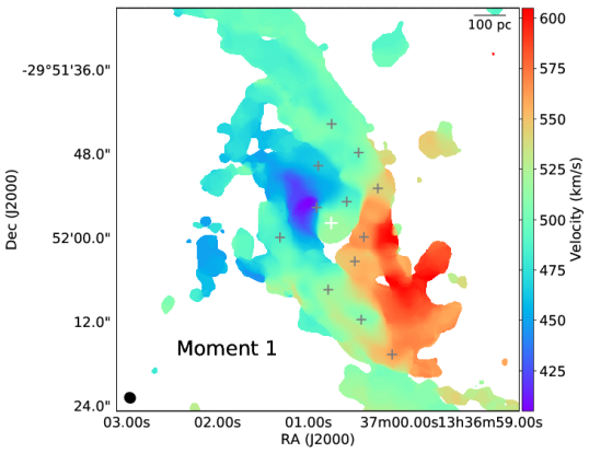
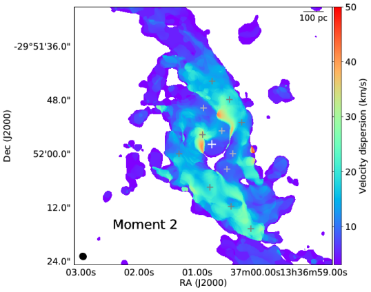
Figure 2: Moment 1 (mean velocity; left figure) and moment 2 (velocity dispersion; right figure) maps obtained from ¹³CO($1-0$) emission. The synthesized beam is shown as a black ellipse on the lower left corner. The position of the center of symmetry is indicated as a white plus sign. Analyzed positions indicated as N1-5, S1-5, and C1-2 in Figure 1 (right) are shown as grey plus signs.

The rotation of the circumnuclear ring is well-traced in the moment 1 map (Figure 2 left). The velocity dispersion shown in the moment 2 map (Figure 2 right) increases from $<10\,$km s^-1 in the bar to $\sim 20\,$km s^-1 when entering into the circumnuclear ring at N1 and S1, likely showing the effect of crowding at orbit intersections leading to cloud collisions. There are two peaks of velocity dispersion with $\sigma\sim 40$ km s^-1; one is near C1, and the other is a position between C2, N2, and N3. The first peak is caused by the motion near the optical nucleus, while the second peak is likely due to double velocity peaks on the line of sight. These double velocity peaks may indicate either two colliding clouds or two clouds that happen to be in the same line of sight, and it is difficult to distinguish between them.

3.2 Spatial variation of molecular emission

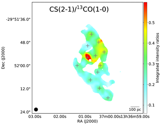
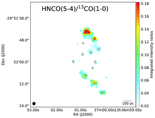
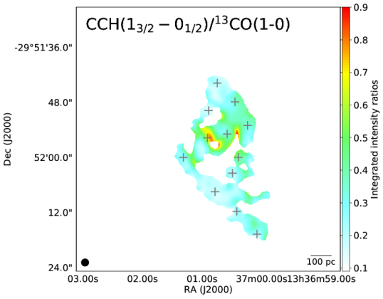
Figure 3: Ratios of line intensities of selected species over that of ¹³CO ($1-0$) in Kelvin scale. Beam sizes are convolved to the same resolution, a larger one between the lines in the numerator and the denominator. All the images are corrected for the primary beam. Ratios of the maximum and the minimum value of the color scale are set to be 10.

We start from examining the spatial variation of the chemistry with the ratio maps of velocity-integrated intensities in Figure 3. All these ratio maps used ¹³CO($1-0$) as the denominator, and were created in the following way. We first made the velocity-integrated intensity maps (moment 0 maps) shown and described in Appendix A. The two images for each ratio map were next convolved to the largest beam among the two images. The image division for ratio was then performed after applying a cutoff at $6\sigma$ and correction for the primary beam to each convolved image.

It is evident from Figure 3 that the distribution of emission vary among different molecular species. Although the C¹⁸O($1-0$)/¹³CO($1-0$) ratio is almost constant throughout the central region of M83 within a factor of 1.6, intensity ratios of some other transitions over ¹³CO($1-0$) have noticable spatial variation.

On the flow coming from the northeast direction (positions N1-5), the CH₃OH ($2_{k}-1_{k}$)/¹³CO($1-0$) ratio has a strong peak at position N1, and the HNCO($5_{0,5}-4_{0,4}$)/¹³CO($1-0$) ratio is enhanced at N1 and N2. Shocks are able to enhance the gas-phase CH₃OH by sputtering off the ice on grains (e.g., Flower & Pineau des Forêts, 2012). Enhanced CH₃OH emission in the large scale is likely to be caused by shocks, because the other mechanism to enhance CH₃OH, thermal evaporation from protostellar cores, can only act in sub-pc scale (e.g., Meier & Turner, 2005; Martín et al., 2006a; Requena-Torres et al., 2006; Harada et al., 2018). HNCO also has a fast formation route on the grain surface, and its abundance is observationally and theoretically shown to be enhanced in shocked regions (Zinchenko et al., 2000; Martín et al., 2008, 2009; Kelly et al., 2017). This N1 position is where the velocity dispersion increases as the gas flows from the bar into the circumnuclear ring, and frequent shocks are expected around there.

The N₂H⁺($1-0$)/¹³CO($1-0$) ratio is also enhanced at N1. Galactic large-scale observations show that N₂H⁺ traces dense cores, even better than conventional “dense-gas tracers” such as HCN and HCO⁺ do (Pety et al., 2017; Kauffmann et al., 2017; Watanabe et al., 2017; Harada et al., 2019) because HCN and HCO⁺ can be sub-thermally excited when they are optically thick. Another explanation is that species such as HCN, HCO⁺, and CS can be excited by collisions with electrons (Liszt & Pety, 2016; Goldsmith & Kauffmann, 2017). On the other hand, N₂H⁺ abundance is theoretically known to increase in the dense environment without the strong influence of UV photons in the model of a collapsing prestellar core (Aikawa et al., 2001). If shocks due to molecular cloud collisions compress gas, this compression increases the dense gas fraction, and can explain the variation of N₂H⁺($1-0$).

The ratio of CCH($1_{3/2}-0_{1/2}$) over ¹³CO($1-0$) does not vary significantly along N1-5 although there is a very slight enhancement at N2 and N3. The CS($2-1$)/¹³CO($1-0$) ratio does not vary significantly either, except for the enhancement at N2. Ethynyl radical (CCH) is thought to be a tracer of PDRs (Pety et al., 2005; Beuther et al., 2008; Martín et al., 2014). CS($2-1$) emission should be rather ubiquitous, but CS emission should come more from relatively denser regions than ¹³CO($1-0$) emission does, due to the higher critical density although excitation from collision with electrons can also contribute if the electron fraction is high.

In the gas flow from the southwestern direction, lines that are enhanced at N1 or N2 with respect to ¹³CO($1-0$) such as CH₃OH ($2_{k}-1_{k}$), HNCO($5_{0,5}-4_{0,4}$), and N₂H⁺($1-0$), have peaks at S2. Other lines such as CCH($1_{3/2}-0_{1/2}$) and CS($2-1$) do not change significantly with respect to ¹³CO($1-0$). As for the central positions, the CCH($1_{3/2}-0_{1/2}$)/¹³CO($1-0$) and CS($2-1$)/¹³CO($1-0$) ratios are enhanced around the optical nucleus (C1). This enhancement may be caused by the lower optical depth of CCH and CS due to the higher velocity dispersion around C1. Because the C1 position is not close to prominent star clusters, enhancement due to PDRs is unlikely.

3.3 Molecular abundances

We derived column densities of species by fitting the spectra at our twelve sampling positions under the assumption of the local thermodynamic equilibrium (LTE). We used the MADCUBA software (S. Martín et al., 2019, submitted) that accounts for the line optical depths and returns column densities and excitation temperatures for the fitted molecules. This analysis used data cubes convolved to 2.8^′′ (62 pc), which is the lowest resolution in our data. While at least two transitions for a species are needed to derive the excitation temperature together with the column density, some species satisfied this condition only at some of our sampling positions. We therefore assumed the following excitation temperatures at positions where only a single transition was detected for each species: CS: $8\pm 2$ K, CCH: $3.5\pm 1.5$ K, N₂H⁺: $6\pm 1$ K, H₂CO: $20\pm 10$ K, HC₃N: $15\pm 10$ K, CH₃CCH: $20\pm 10$ K. These temperatures are from positions with successful $T_{ex}$ fitting, and we assumed them to have fixed ranges because excitation temperatures did not vary significantly among positions for species with multiple transitions detected at all positions. For C¹⁷O, we only observed $J=2-1$ in our settings, and assumed its excitation temperature to be similar to those of C¹⁸O and ¹³CO at each position. If a species has both ortho and para states such as H₂CO, we used the ortho-to-para ratio of 3, which is the value of the statistical weight. This ortho-to-para ratio is achieved when the thermal equilibrium is achieved and the temperature is high compared with the energy differences between ortho and para states. This assumption of ortho-to-para ratio is justified in the warm environment of our observations, a galactic center in a starburst galaxy.

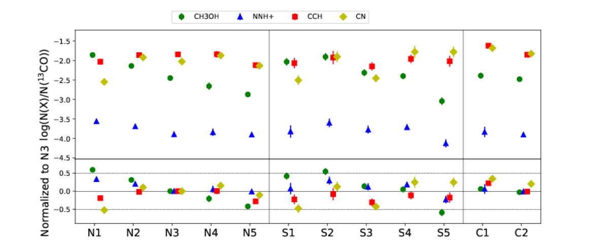
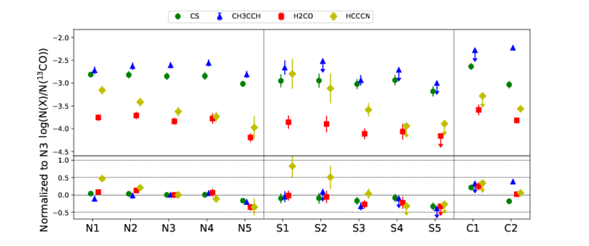
Figure 5: Column density ratios of molecular species over that of ¹³CO for each position (Top panels). Bottom panels show the same quantities, but are normalized to the values at N3.

The upper panel of Figure 5 shows the column density ratios of selected species over ¹³CO for positions in the northeastern stream (N1-5), the southwestern stream (S1-5), and central positions (C1-2). The lower panel shows the same values normalized to N3. For simplicity, we refer to the column density ratios as fractional abundances, assuming that the ¹³CO fractional abundance does not vary among positions.

For the northeastern stream (N1-N5), the change in fractional abundances from N1 can be categorized into monotonic increase, no change, or decrease along the stream. Most species decrease in fractional abundances such as CH₃OH, N₂H⁺, and HC₃N. The largest change from the upstream to the downstream is seen in CH₃OH, and it is by a factor of $\sim 10$ while the change is only a factor of $\sim 2$ for N₂H⁺. The fractional abundances of C₂H, CS, CH₃CCH, and H₂CO show little change along the northeastern stream except at N5, where H₂CO is about 3 times less abundant than that at other positions. The fractional abundance of CN is the lowest at N1, $\sim 4$ times higher at N2, and stays constant further downstream.

In contrast to the northeastern stream, most of the species in the southwestern stream (S1-S5) do not show simple monotonic increase or decrease in fractional abundances; they rather fluctuate within the stream. An exception is CH₃OH, whose fractional abundance monotonically decreases along the southwestern stream as it does in the northeastern stream.

The two peaks in the central region C1 and C2 show little difference from other positions in their chemical compositions. Exceptions are C1 and C2 having higher CN fractional abundances compared with the peaks in the northeastern and southwestern streams, and C2 having the highest CH₃CCH fractional abundances among all positions.

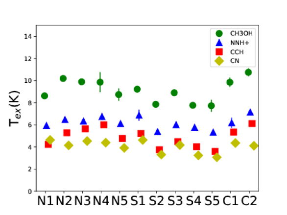
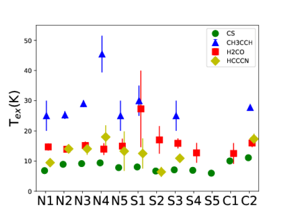
Figure 7: Excitation temperatures derived from our analysis. Values are not shown if only one transition of the particular molecule was detected.

Our derived excitation temperatures are shown in Figure 7. For most species, the excitation temperatures do not vary significantly from position to position, and hence intensity ratios are relatively good measures of column density ratios of our observed molecules. Despite the invariance between positions, there are differences of excitation temperatures between species. Such variations have also been reported in other external galaxies (e.g., Martín et al., 2006b; Aladro et al., 2011; Nakajima et al., 2018) This variation between species is likely because each species emit from different components within the observed beam. Exact values of column densities derived from our results are listed in Tables 4 - 6.

3.4 Intensity ratios

We also analyzed species with only one transition in our observations and a radio recombination line H41$\alpha$ for their variation among our twelve positions in intensity ratios with respect to ¹³CO$(1-0)$. Figure 6 shows the ratios and ratios normalized to the values at N3, all for the 2.8^′′ resolution. HNC does not show evident spatial variation except for lower fractional abundances in the downstream (N5 and S5) by a factor of a few. The variation of CH₃CN fractional abundance is not evident either because there are non-detections in some positions. Meanwhile, SiO and H41$\alpha$ show hints of spatial variation. $I({\rm SiO})/I(^{13}{\rm CO})$ is more than a factor of 3 higher at N1 than at N3. When comparing S1 and S3, the enhancement of $I({\rm SiO})/I(^{13}{\rm CO})$ at the upper stream, i.e., S1, is less obvious. SiO is known to be formed when Si is ejected from grains because of fast shocks (Martin-Pintado et al., 1992; Gusdorf et al., 2008; Flower & Pineau des Forêts, 2012), and this variation may be caused by the difference in the frequency of strong shocks.

It is not straightforward to interpret the variation of H41$\alpha$ intensity ratios because H41$\alpha$ is detected only at N2 and N3 and we could only get high upper limits for some of other positions. Yet, the difference between the northeastern stream and southwestern stream can be highlighted by the difference between N3 and S3, the locations with the highest ¹³CO column densities in each stream. The intensity ratio $I({\rm H41\alpha})/I(^{13}{\rm CO})$ is more than a factor of 3 higher at N3 than at S3, with only an upper limit obtained at S3. Radio recombination lines from ionized gas trace high-mass star formation. Therefore, this difference suggests a higher star formation rate and a higher star formation efficiency in the northeastern stream than in the southwestern stream. Observed intensities in the analyzed positions are listed in Table 7.

4 Discussion

4.1 A scenario proposed for the chemical variation in the northeastern stream

The chemical variation we reported in Sections 3.2 - 3.4 is as follows. At the upstream positions N1 and N2, CH₃OH fractional abundance and the intensity ratio of SiO/¹³CO are higher than at other positions. These species are known to be enhanced with shocks. The fractional abundance of N₂H⁺ is also elevated at N1 and N2. It is known that the N₂H⁺ fractional abundance is enhanced in dense regions. On the other hand, the CN fractional abundance increases from N1 to N2 by about a factor of 3, and stay at similar values towards downstream, while CCH fractional abundance does not change along the northeastern stream. Similar to CCH, CN is known to be a PDR tracer (Fuente et al., 1993). The hydrogen recombination line H41$\alpha$ is clearly detected around N2 and N3 although there is no detection at other positions.

Here we note that the changes in derived fractional abundances or intensity may correspond to changes in the fraction of the gas that are shocked, dense, or UV-irradiated within the beam.

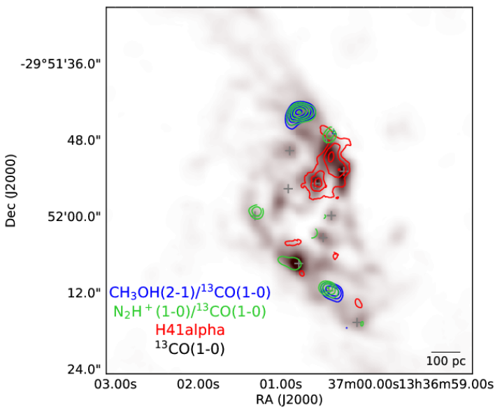
Figure 8: (Left) A schematic image of our proposed scenario. The background image is a moment 0 map of ¹³CO($1-0$). (Right) Contours of CH₃OH(2-1)/¹³CO(1-0) velocity-integrated intensity ratio shown in blue, N₂H⁺/¹³CO(1-0) velocity-integrated intensity ratio in green, and H41$\alpha$ velocity-integrated intensity in red overlaid on a moment 0 map of ¹³CO($1-0$).

From the variation observed in the northeastern stream, we propose the following scenario (Figure 8). N1 is the entering point of the gas from the bar orbit into the circumnuclear ring, dominated by frequent hydrodynamical shocks. These shocks can explain the increase of CH₃OH abundance and SiO intensity at N1 and N2. At these positions, N1 and N2, the velocity dispersion is slightly higher ($\sim 15\,$km s^-1) than to the north of N1 ($v_{\rm disp}<10\,$km s^-1). This is consistent with our inference that there must be shocks at these positions. These shocks must also have increased the fractional abundance of N₂H⁺ because the compression of colliding molecular clouds should increase the gas density. This downstream compression may explain the active star formation between N2 and N3 seen in H41$\alpha$ (Figure 5). The increase of CN fractional abundance downstream agrees with the higher star formation rate at N2 and N3, but the invariance of the CCH fractional abundance along the stream cannot be explained if the CCH fractional abundance directly reflects the strength of the interstellar radiation field. There are various claims how the CCH abundance depends on the UV-radiation strength. Meier & Turner (2005) found in the circumnuclear ring of IC 342 that CCH peaks do not coincide with young ($\sim$ a few Myr old) star-forming regions in two of the giant moelcular clouds on the ring. They deduced that the effect of the still embedded young stars are too localized and minimized to have CCH peaks. Model calculations by Aladro et al. (2013) showed that CCH abundance is rather insensitive to the UV field. On the other hand, results by Martín et al. (2014) seem to show CCH enhancement over HCN, HCO⁺, and HNC due to young star formation in an isolated star-forming galaxy in CIG 638.

4.2 Timescales of collision-induced star formation

4.2.1 Orbital timescale

For the proposed scenario of collision-induced star formation to be plausible, the timescale of the gas moving from N1 to N3 should be reasonable for star formation to take place. The timescale can be estimated from the orbital timescale and the positional offset between N1 and N3. We estimated the orbital timescale for a gas cloud to go around once on the circumnuclear ring as follows. The difference between the maximum line-of-sight velocity on the circumnuclear ring and the mean line-of-sight velocity of the ring $v_{los}$ is estimated to be $70\pm 10$ km s^-1 on our moment 1 map. With the inclination angle of 24^∘(Comte, 1981), the unprojected velocity $v=v_{los}/{\rm sin}(24^{\circ})$ is $172\pm 25$ km s^-1. From our molecular emission map, the radius of the circumnuclear ring $R$ is estimated to be $250\pm 25$ pc. The angular velocity of the gas in the circumnuclear ring $\Omega$ is $\Omega=v/R=690\pm 120$ km s^-1 kpc^-1. Because the pattern speed of the bar $\Omega_{p}$ is $57\pm 3$ km s^-1 kpc^-1 (Hirota et al., 2014), the angular speed of a cloud in the circumnuclear ring with respect to the ring structure is $\Omega-\Omega_{p}=630\pm 120$ km s^-1 kpc^-1. The orbital period $\tau$ is obtained as $\tau=\frac{2\pi}{\Omega-\Omega_{p}}=10\pm 2$ Myr. This orbital period means that it only takes a few Myr for a cloud to travel from the initial shock at N1 to star formation at N3.

4.2.2 Collision timescale

If star formation is triggered at the orbit intersection through cloud collisions, the collision timescale plus the star formation timescale should be as short as a few Myr for our proposed scenario viable. The collision timescale of molecular clouds in spiral arm regions is estimated to be 8-10 Myr (Dobbs et al., 2015). However, we expect the collision timescale to be much shorter in the area of our observations because it is at the galactic center region with much higher number density of molecular clouds, and because the orbit intersection increases the chance of collision.

An order-of-magnitude estimation of the timescale of collisions can be made by considering the mean free path and the velocity (or velocity dispersion) of molecular clouds. The mean free path of a cloud is $l=\frac{1}{n_{cl}\sigma}$ where $l$ is the mean free path, $n_{cl}$ is the number density of the collision partner, and $\sigma$ is the cross section of the collision partner. Then, the timescale of the collision is $t\sim\frac{1}{n_{cl}\sigma v}$ where $v$ is the velocity of the cloud with respect to the collision partner. After the calculation described in Appendix C, we obtain

$$t\sim{\rm 1.6\,Myr}~{}\left(\frac{R_{cl}}{\rm 20\,pc}\right)^{-2}\left(\frac{M_{cl}}{1.5\times 10^{5}M_{\odot}}\right)\left(\frac{v}{\rm 20\,km\,s^{-1}}\right)^{-1},$$ (1)

where $R_{cl}$ and $M_{cl}$ are the radius and the mass of a giant molecular cloud (GMC), respectively. Here we assume the mass and the radius of a GMC to be that of typical Galactic GMCs (Heyer et al., 2009; Leroy et al., 2015). This derived value of collision timescale is only a small fraction ($\sim 16\%$) of the orbit timescale. Those frequent inelastic collisions can reduce the velocity dispersion within the stream, and the collision frequency gradually decreases. The change in collision frequency can reduce the fractional abundances of shock tracers as discussed below.

4.2.3 Timescale of chemical variation

We find that fractional abundances of shock tracers vary gradually along the orbit. Here we discuss how this gradual change is caused considering the timescale of chemical and physical processes. The timescale of CH₃OH and SiO to freeze onto dust grains is $\sim 10^{9}/n$ yr, relatively short for moderately dense gas ($\lesssim 10^{5}$ yr for $n\gtrsim 10^{4}$ cm^-3) (Caselli et al., 1999). Because the orbital timescale of the circumnuclear ring is around 10 Myr, its size is around 500 pc in diameter, and our angular resolution is in the order of 10 pc, we should observe no spatial shift between the location of shocks and the location of enhancement of shock tracers. That is, shock tracers are only seen locally close to the location of shocks. In other words, the observed gradual variation of chemical abundances suggests gradual variation in the frequency of shocks.

4.2.4 Timescale of star formation

From the fast variation of the chemistry of shock tracers, we consider that the collision timescale is relatively short $\sim 1$ Myr. After a collision, the timescale of the star formation can be compared with the free fall time, $\tau_{ff}={3\times 10^{5}}\left(\frac{n}{10^{4}{\rm\,cm^{-3}}}\right)^{-1/2}$ yr. The star formation usually takes place in the free-fall time or longer. This timescale is shorter than the time it takes for the gas to move from N1 to N3 when $n\gtrsim 10^{3}$ cm^-3. If the star formation at N3 is induced by a collision at N1, the collision must have compressed the gas to $n=10^{3}-10^{4}$ cm^-3. We leave it to theoretical studies whether this level of compression is reasonable or not. Meanwhile, there are indeed Galactic star formation regions where collisions seem to have triggered star formation within $\lesssim 1$ Myr (Torii et al., 2011; Fukui et al., 2014, 2018).

Information on stellar ages at N2 and N3 can confirm the scenario of collision-induced star formation if they have ages around 2-3 Myr. Age-dating of starburst has also been conducted for star clusters in and around the circumnuclear ring of M83. However, most young clusters are located in regions that are unobscured in optical or NIR wavelength, and their ages are in the range of 5-10 Myr (Harris et al., 2001; Houghton & Thatte, 2008; Knapen et al., 2010). Although Knapen et al. (2010) reported that there is a gradient of stellar ages in clusters near N2, N4, and N5 clouds with ages of 5.5, 6.8, and 8.6 Myr, their observations likely did not trace stars formed at the orbit intersection on the northeastern stream if they travel on the circumnuclear ring with the orbital period of 10 Myr. There are a few clusters with ages of a few Myr around the N2 cloud in the observations by Harris et al. (2001), but there is no work reporting the ages of obscured star formation around the N2 and N3 clouds that we observe with radio recombination lines. Therefore, these studies on stellar ages cannot be used to confirm the scenario of collision-induced star formation.

With the consideration of factors discussed in Sections 4.2.1 - 4.2.4, we conclude it plausible that the star formation around N2 & N3 was triggered by the collisions at the orbit intersection if these collisions can compress the gas up to $n=10^{3}-10^{4}$ cm^-3 or higher.

4.3 Comparison between the northeastern stream and the southwestern stream

As explained in Section 3.3, there is difference between the chemical composition in the northeastern and southwestern streams. The enhanced fractional abundance of methanol at S1 and S2 suggests that there are shocks at the orbit intersection in the southwestern stream, which is similar to the case in N1. On the other hand, the SiO/¹³CO intensity ratio is lower at S1 or S2 than at N1 and N2. Because SiO is known to be enhanced with strong shocks ($>25$ km s^-1 Gusdorf et al., 2008), strong shocks must be more frequent in the northeastern stream. On the southwestern stream, there is no sign of active star formation traced by the radio recombination line, either.

There are a few possible reasons for this lack of star formation in the southwestern stream. One possible reason is the lack of the gas supply. As it is obvious from the moment 0 maps (e.g., ¹³CO($1-0$) map in Figure 9), the distribution of the molecular gas is not uniform along the circumnuclear ring. If the gas inflow from the bar has been scarce in the southwestern stream in the past few Myr or so, this lack of fresh gas supply suppresses star formation. If this is the case, the gas currently located at S1-S3 may result in star formation in a few Myr as the clouds reach the intersection with the nuclear ring. Another possible reason is the lack of strong shocks. Although CH₃OH fractional abundance is moderately enhanced at S1-S2 and the moment 2 map shows higher velocity dispersion at S1 compared with the upstream, there is less emission of SiO in the southwestern stream. This trend indicates that strong shocks are less frequent there. On the other hand, the velocity dispersion shown in the moment 2 map (Figure 2 right) is slightly larger in the southwestern stream. More turbulence on the southwestern stream can also restrain star formation. Although it seems contradictory to the less SiO intensity on the southwestern stream, the southwestern stream may have more turbulence with low-velocity shocks. There is yet another possible scenario where the collision-induced star formation is not the major mode of star formation. Seo & Kim (2013) proposed that collision-induced star formation does not provide as high star formation rate as star formation due to self gravity within the circumnuclear ring when the gas inflow rate is large. It is because the gas flows through the orbit intersection without colliding. However, this scenario is unlikely in this particular case of the southwestern stream of M83 because the gas is more scarce on this stream than on the northeastern stream. The column densities of ¹³CO at S1 and S2 are about a half of the column densities at N1 and N2.

4.4 Other contributing factors to the chemical composition

In addition to the chemical processes discussed in our proposed scenario in Section 4.1, there are other factors contributing to the chemistry. First, we discuss the case of PDR tracers. Although CCH and CN have been claimed to be PDR tracers, their fractional abundances depend not only on the UV-field strength, but also on the gas volume density because reactions involving UV photons become more effective in lower-density environments. Theoretical studies have shown that the quantity $G_{0}/n$ is the control parameter of PDR chemistry (e.g., Draine & Bertoldi, 1996) where $G_{0}$ is the UV-field strength. This dependence on the density has also been discussed in Martín et al. (2015) in the context of extragalactic chemical observations. Our results show that the fractional abundances of CCH are almost constant among positions. If the emission of CCH comes from low-density regions of molecular clouds, even clouds without star formation can emit some amount of CCH. This may explain why the fractional abundances of CCH do not necessarily correlate with the strengths of star formation.

Unlike PDR tracers, some species are more prone to dissociation by UV-photons. One example is methanol. We proposed that the enhancement of CH₃OH at N1 is caused by more frequent shocks than at downstream positions. However, the decreased abundances of methanol at N2 or N3 may be caused by photodissociation from the star formation there. On the other hand, the enhanced CH₃OH/¹³CO at the entering point from the bar is also seen on the southwestern stream, where there is no obvious star formation. Therefore, it is likely that some methanol emission is still enhanced due to shocks.

Abundances of some species may also be affected by changes in the temperature of dust grains. For example, when the dust grains are warm, the production rate of methanol is suppressed. Such heating of dust may be effective in active star-forming regions. The N₂H⁺ fractional abundances may also be affected by the dust temperature because CO may be less depleted on warm dust grains and there is a major destruction route of N₂H⁺ through CO (Bergin et al., 2001).

4.5 Comparison with other galactic centers

There are galactic centers that show chemistry similar to the one in M83 and there are ones that do not. Our proposed scenario is similar to what was suggested by Meier & Turner (2005) for IC 342. The enhancement of CH₃OH and N₂H⁺ at the bar-ring orbit intersections was also seen in IC 342.

As mentioned earlier, NGC 1097 is an example where star formation seems independent from the galactic orbits. Martín et al. (2015) studied the circumnuclear ring of NGC 1097 for the spatial abundance variation of such species as SiO, CCH, HCN, HCO⁺, HNCO, CS, SO, and HC₃N. Unlike our results in M83, there is no large variation of the chemical composition in the circumnuclear ring of NGC 1097 except for CCH. This difference may be caused by the presence of collision-induced star formation in M83, although we caution that a similar large scale chemical variation due to cloud collision may be present also in NGC 1097 at a low level below the sensitivity of their cycle 0 observations. In the case of NGC 1097, the scenario by Seo & Kim (2013) may be relevant because of the high gas inflow rate.

Mills & Battersby (2017) analyzed the chemical composition of the Galactic central molecular zone (CMZ) using the survey data by Jones et al. (2012). They analyzed ratios of molecular line intensities with respect to the total column density of the molecular gas. Spatial variation of these ratios should reveal the variation of fractional abundances of those species provided that the excitation temperature is constant. The interpretation of these data in relation with the galactic orbits is more difficult in the Galactic Center than in M83 because of the edge-on configuration of our Galaxy. There are models of Galactic Center structure to explain the observed position-velocity diagram (e.g., Sawada et al., 2004; Kruijssen et al., 2015). According to the model by Sawada et al. (2004), the $1.3^{\circ}$ cloud is at the orbit intersection from the bar to the circumnuclear ring. SiO is indeed enhanced in the $1.3^{\circ}$ cloud and the $1.6^{\circ}$ cloud as seen in Riquelme et al. (2010) from the SiO/H¹³CO⁺ intensity ratio. In Mills & Battersby (2017), the enhancement in the $1.3^{\circ}$ cloud and the $1.6^{\circ}$ cloud was not seen because their analysis only included regions above a certain column density threshold, and these clouds have column densities below the threshold. Therefore, the SiO fractional abundance is highest in Sgr B2 in Mills & Battersby (2017). Sgr B2 clouds were suggested to be under the influence of tidal compression in the model by Kruijssen et al. (2015), and frequent shocks may also be relevant there. N₂H⁺ is also most enhanced in Sgr B2 according to the map by Mills & Battersby (2017). Partly because of the edge-on configuration, we are unable to see similarity of the chemistry of the Galactic Center CMZ with that of M83 except for frequent shocks at the 1.3^∘ cloud.

5 Summary

We have presented multi-species, multi-transition ALMA observations in the galactic center region of M83. We have studied the variation of chemistry as the gas flows from the bar into the circumnuclear ring and moves to the star-forming regions. Here are the summary of our results.

• Shock tracers (SiO and CH₃OH) are found to be enhanced at the two locations where the leading-edge gas lanes on the bar are connected to the circumnuclear ring.

• In the northeastern stream, the N₂H⁺ fractional abundance decreases as the gas travels further from the orbit intersection. This variation in the fractional abundance indicates gas compression at the orbit intersection if N₂H⁺ emission preferentially comes from dense gas. Signs of active star formation are seen from the radio recombination line H41$\alpha$ and CN further downstream. This variation can be explained by the star formation induced by the collisions of molecular clouds at the orbit intersection and by the gas compression through the collisions.

• If the star formation in the northeastern stream is indeed triggered at the orbit intersection, the timescale of star formation is 2-3 Myr. The collision frequency at the orbit intersection is estimated to be on the order of $\sim 1$ Myr, and star formation within a few Myr is possible if the gas compression is effective enough to allow gravitational collapse in a short timescale on the order of 1 Myr.

• The southwestern stream lacks the sign of gas compression and star formation. This difference from the northeastern stream may come from the lower amount of gas in the southwestern stream, or the lack of strong shocks.

• The chemistry in the center of M83 and its dependence on the galactic structure is similar to what was observed in IC 342. On the other hand, the chemical variation of M83 shows little similarity with that in the circumnuclear ring of NGC 1097.

We have shown here that astrochemistry can be used to study collision-induced star formation in nearby galaxies. At the same time, it is still unclear what the exact cause is for presence or absence of collision-induced star formation. Further astrochemical studies in a larger sample may help resolving the condition for the collision-induced star formation and revealing more of the ISM evolution related to galactic gas dynamics.

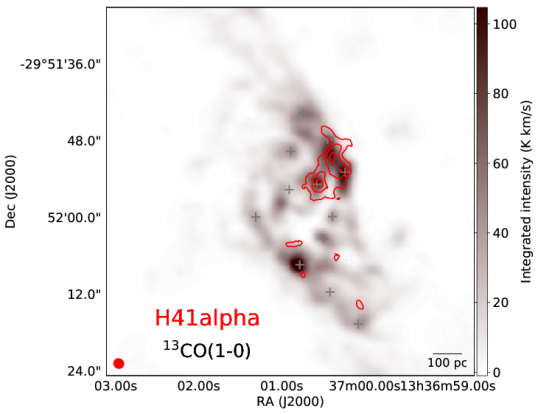
Figure 4: Velocity-integrated intensity map of H41$\alpha$ (red contours) overlaid on the velocity-integrated intensity map of ¹³CO(1-0) (grey scale). The contour levels of H41$\alpha$ are every 0.96 K km s^-1 with the typical rms of 0.32 K km s^-1 (see details of moment 0 maps in Appendix A).

Figure 6: Intensity ratios of molecular emission over that of ¹³CO ($1-0$) (Top panels). Bottom panels show the same quantities, but are normalized to the values at N3.

Appendix A Velocity-integrated intensity maps

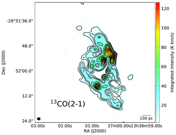
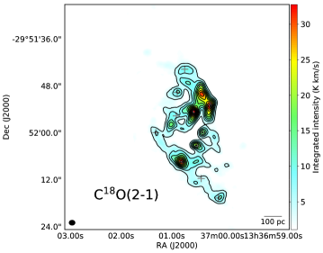
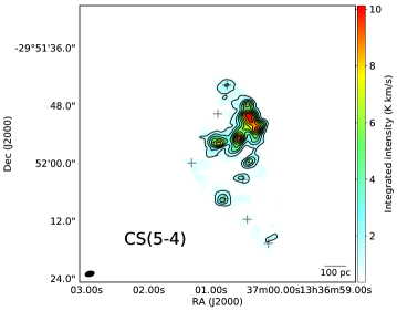
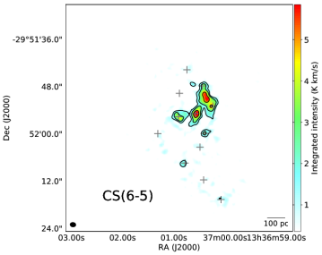
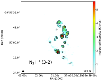
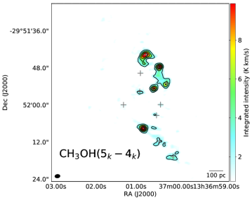
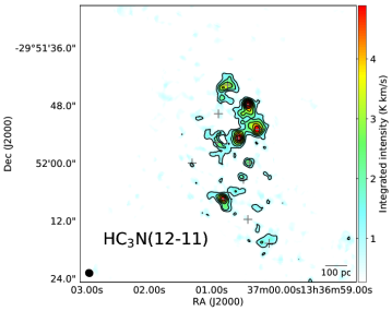
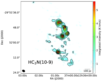
Figure 10: Same as Figure 9, but for other lines. Contour levels are plotted at 7.6, 15.1, 22.7, and every 15.1 K km s^-1 for ¹³CO($2-1$) with $\sigma_{\rm N1}=0.53$ K km s^-1, every 3.6 K km s^-1 for C¹⁸O($2-1$) with $\sigma_{\rm N1}=0.31$ K km s^-1, every 0.6 K km s^-1 for C¹⁷O($2-1$) with $\sigma_{\rm N1}=0.20$ K km s^-1, every 1.4 K km s^-1 for CS($5-4$) with $\sigma_{\rm N1}=0.19$ K km s^-1, 1.2, 2.3, 3.5, and every 2.3 K km s^-1 for CS($6-5$) with $\sigma_{\rm N1}=0.26$ K km s^-1, 1.1, 2.2, 3.3, and every 2.2 K km s^-1 for N₂H⁺($3-2$) with $\sigma_{\rm N1}=0.37$ K km s^-1, every 2.2 K km s^-1 for CH₃OH($5_{k}-4_{k}$) with $\sigma_{\rm N1}=0.27$ K km s^-1, every 0.8 K km s^-1 for HC₃N($12-11$) with $\sigma_{\rm N1}=0.41$ K km s^-1, and every 0.8 K km s^-1 for HC₃N($10-9$) with $\sigma_{\rm N1}=0.34$ K km s^-1.

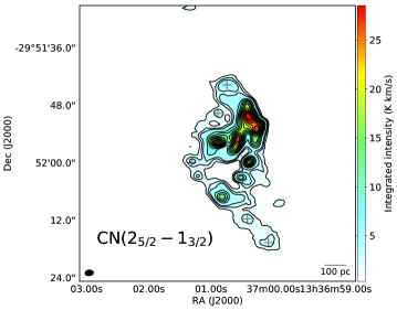
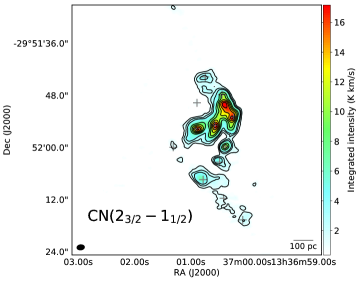
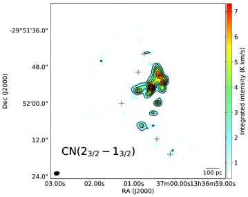
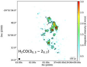
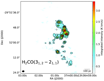
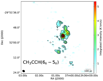
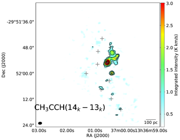
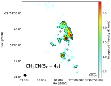
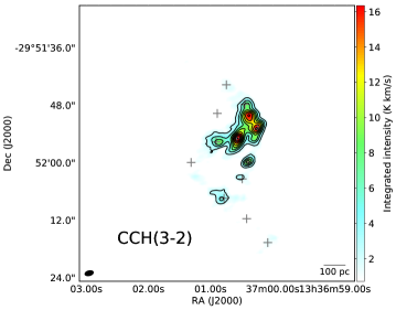
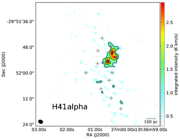
Figure 11: Same as Figure 9, but for other lines. Contour levels are plotted at 1.6, 3.1, 4.7, and every 3.1 K km s^-1 for CN($2_{5/2}-1_{3/2}$) with $\sigma_{\rm N1}=0.16$ K km s^-1, 1.8, 3.6, 5.4, and every 3.6 K km s^-1 for CN($2_{3/2}-1_{1/2}$) with $\sigma_{\rm N1}=0.18$ K km s^-1, and every 1.7 K km s^-1 for CN($2_{3/2}-1_{3/2}$) with $\sigma_{\rm N1}=0.18$ K km s^-1, every 1.0 K km s^-1 for H₂CO($3_{0,3}-2_{0,2}$) with $\sigma_{\rm N1}=0.32$ K km s^-1, every 0.6 K km s^-1 for H₂CO($3_{1,2}-2_{1,1}$) with $\sigma_{\rm N1}=0.20$ K km s^-1, every 1.0 K km s^-1 for H₂CO($4_{1,4}-3_{1,3}$) with $\sigma_{\rm N1}=0.22$ K km s^-1, 0.96, 1.9, 2.8, and every 1.9 K km s^-1 for CH₃CCH($6_{k}-5_{k}$) with $\sigma_{\rm N1}=0.32$ K km s^-1, 0.7, 1.4, 2.1, and every 1.4 K km s^-1 for CH₃CCH($14_{k}-13_{k}$) with $\sigma_{\rm N1}=0.23$ K km s^-1, every 0.8 K km s^-1 for CH₃CN($5_{k}-4_{k}$) with $\sigma_{\rm N1}=0.34$ K km s^-1, every 2.3 K km s^-1 for CCH($3-2$) with $\sigma_{\rm N1}=0.22$ K km s^-1, and every 0.96 K km s^-1 for H41$\alpha$ with $\sigma_{\rm N1}=0.32$ K km s^-1.

Figures 9-11 show velocity-integrated intensity maps in our observations. To create moment 0 maps with as high signal-to-noise ratios as possible, we masked out the region with ¹³CO emission below 5 $\sigma$ in each velocity channel. This mask was applied to line cubes of all isolated lines, and velocity-integrated intensity maps were created with the task immoments. A number of species show multiple transitions contributing to the observed line profile (e.g. the hyperfine structure of CN or CCH) For those lines, we made masks with velocity shifts corresponding to those transitions. The intersection of those masks was applied to the cube as a new mask. Because of the use of masks, the noise levels are not constant within the map. The error in the velocity-integrated maps can be estimated as $\sigma_{\rm integ}=\sigma_{1ch}\Delta v_{ch}\sqrt{N}$ where $N$ is the number of channels integrated and $v_{ch}=10$ km s^-1 is the width of one channel. If there is no blending of multiple transitions, the number of channels integrated over at analyzed positions are N1 : 9, N2 : 12, N3 : 12, N4 : 8, N5 : 6, C1 : 17, C2 : 13, S1 : 10, S2 : 11, S3 : 11, S4 : 9.6, S5 : 7. To obtain the number of channels used for the images with multiple transitions integrated together, add 10 to those numbers in the isolated line case for CN ($N=2-1,J=3/2-3/2$), 9 for CN ($N=2-1,J=3/2-1/2$), 2 for CN (N=2-1,J=5/2-3/2), 4 for CCH($N=1-0,J=3/2-1/2$), 2 for CCH ($N=1-0,J=1/2-1/2$), 7 for CCH ($N=3-2$), and 22 for CH₃OH ($5_{k}-4_{k}$).

Appendix B Continuum emission

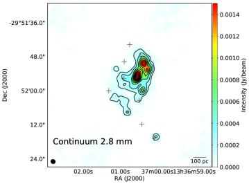
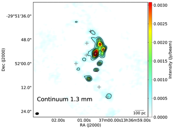
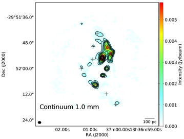
Figure 12: Continuum images of the central region of M83 at 2.8, 1.3, 1.0 mm. Images are produced using line-free channels of one sideband (3.65-GHz wide). The contour levels are 6, 12, 18, 24, and every 12 $\sigma$ for 2.8mm ($1\sigma=25\,\mu$Jy beam^-1), 6, 12, 18, 24, 30, 36, and every 12 $\sigma$ for 1.3 mm ($1\sigma=77\,\mu$Jy beam^-1) , and 6, 12, 18, 24, and every 12 $\sigma$ for 1.0 mm ($1\sigma=100\,\mu$Jy beam^-1). The synthesized beams are shown as black ellipses on the lower left corner, and their sizes are $1.8^{\prime\prime}\times 1.7^{\prime\prime}$ for 2.8 mm, $1.8^{\prime\prime}\times 1.3^{\prime\prime}$ for 1.3 mm, $1.6^{\prime\prime}\times 1.3^{\prime\prime}$ for 1 mm.

Figure 12 shows the maps of continuum emission at 2.8, 1.3, and 1.0 mm. The areas we detected the continuum emission are smaller than those for major molecular lines such as CO isotopologues. There is also visible difference between the continuum emission of 2.8 mm and those at 1.3 and 1.0 mm. This is most likely because the former has a sizable contribution from free-free and synchrotron emission while the latter is dominated by dust emission.

We estimate the contribution of free-free emission to the continuum emission in Band 3 from the flux of the radio recombination line H$41\alpha$, which turns out to be 45-100 %. We used a formula from Brown et al. (1978) to estimate the free-free continuum intensity from the observed H$41\alpha$ intensity,

$$\int T_{L}dv/T_{c}=6.76\times 10^{3}\nu^{1.1}T_{e}^{-1.15},$$ (B1)

where $\int T_{L}dv$ is the velocity-integrated intensity of a radio recombination line, $T_{c}$ is the intensity of continuum from free-free emission, $\nu$ is the frequency in the unit of GHz, and $T_{e}$ is the electron temperature. Within the area of H41$\alpha$ emission, the averaged H41$\alpha$ velocity-integrated intensity is 0.94 K km s^-1, and the continuum intensity is 0.029 K. We obtained the fractional contribution of the free-free emission using the range of electron temperatures $T_{e}=4000-10^{4}$ K from values in Galactic sources or in a starburst galaxy (Shaver et al., 1983; Paladini et al., 2004; Bendo et al., 2015). Presence of significant free-free emission explains different spatial distribution of continuum emission between Band 3 and Bands 6 and 7. The continuum intensities are significantly larger in the higher-frequency bands, which must be due to dust emission.

Appendix C Estimate of collision frequency

The collision time scale is estimated as $t\sim\frac{1}{n_{cl}\sigma v}$ where $v$ is the velocity of the cloud with respect to the collision partner, and $n_{cl}$ is the number density of clouds. Meanwhile, the volume filling factor $\Phi$ can be expressed as $n_{cl}V_{cl}$ where $V_{cl}$ is the volume of a single molecular cloud. If we assume a spherical cloud with a radius $R_{cl}$, the collision time scale can be expressed as $t\sim\frac{4}{3}\frac{R_{cl}}{\Phi v}.$ Here we estimate the volume filling factor as follows. We assume the stream is flowing in a cylindrical structure with a radius of $r$ and a length of $l$. Consider the number of molecular clouds within this cylinder to be $N_{cl}$, and the total volume of the cylinder to be $V_{tot}$. Then, $\Phi=\frac{N_{cl}V_{cl}}{V_{tot}}.$ If we define $M_{tot}$ as the total gas mass in the volume and $M_{cl}$ as the mass of a single cloud, we can express $N_{cl}$ as $N_{cl}=\frac{M_{tot}}{M_{cl}}$. $M_{tot}$ can also be expressed as $M_{tot}=m_{H2}N_{H2}A$ where $A=2rl$ is the area of the cylinder seen from the side, $m_{H2}$ is the mass of one hydrogen molecule, and $N_{H2}$ is the averaged ${\rm H_{2}}$ column density of the cylinder seen from the side. Because $V_{cl}=\frac{4}{3}\pi R_{cl}^{3}$ and $V_{tot}=\pi r^{2}l$, we can rewrite the volume filling factor as $\Phi=\frac{8}{3}\frac{m_{H2}N_{H2}R_{cl}^{3}}{M_{cl}r}$. From our data, the average column density of ¹³CO over $r=55$ pc ($2.5^{\prime\prime}$) is $N_{13CO}\sim 2\times 10^{16}$ cm^-2. Assuming the $N_{13CO}=10^{-6}N_{H2}$, $R_{cl}=20$ pc, and $M_{cl}=1.5\times 10^{5}$ $M_{\odot}$, we obtain $\Phi=0.77\left(\frac{R_{cl}}{20pc}\right)^{3}\left(\frac{M_{cl}}{1.5\times 10^{5}M_{\odot}}\right)^{-1}\left(\frac{N_{H2}}{2\times 10^{22}{\rm cm^{-3}}}\right)\left(\frac{r}{55pc}\right)^{-1}$ .

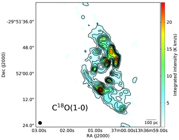
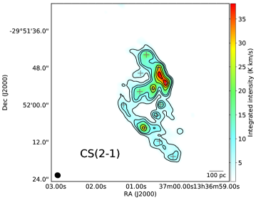
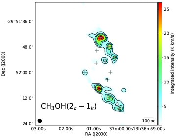
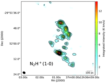
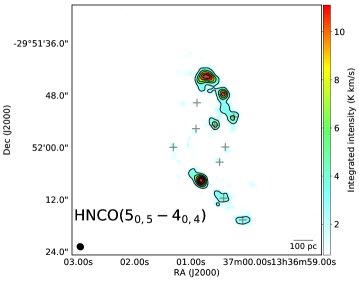
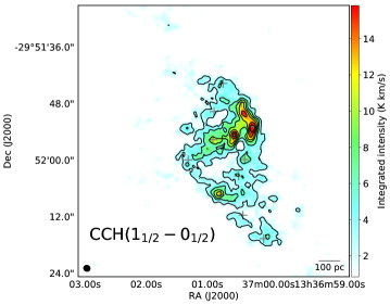
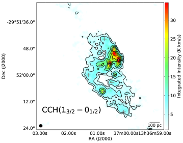
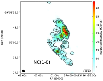
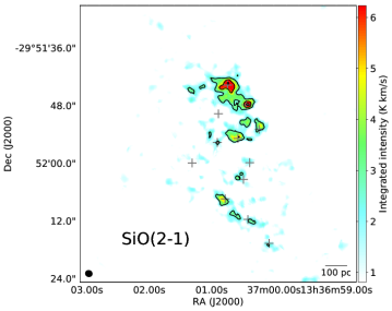
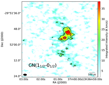
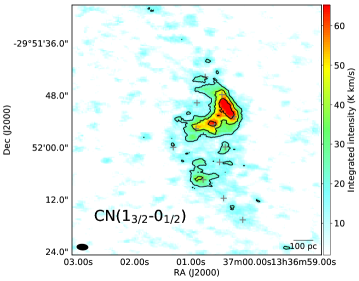
Figure 9: Velocity-integrated intensity maps of some of the detected lines before the primary beam correction. The analyzed positions N1-5, S1-5, and C1-2 are shown as grey plus signs. The synthesized beam is shown as a black ellipse on the lower left corner. Their beam sizes are listed in Table 2. The noise level spatially varies in each map because the number of integrated channels varies with position due to our masking. The noise at the N1 position is listed below as $\sigma_{\rm N1}$. See Appendix A to obtain the noise at other positions. Contour levels are plotted at 5.9, 11.8, 17.6, and every 11.8 K kms^-1 for ¹³CO($1-0$) with a typical noise of $\sigma_{\rm N1}=0.56$ K km s^-1, 1.7, 3.5, 5.2, 7.0, 8.7, and every 3.5 K km s^-1 for C¹⁸O($1-0$) with $\sigma_{\rm N1}=0.44$ K km s^-1, 3.4, 6.7, 10.1, and every 6.7 K km s^-1 for CS($2-1$) with $\sigma_{\rm N1}=0.34$ K km s^-1, 3.2, 6.5, 9.7, and every 6.5 K kms^-1 for CH₃OH($2_{k}-1_{k}$) with $\sigma_{\rm N1}=0.33$ K km s^-1, every 2.1 K kms^-1 for N₂H⁺($1-0$) with $\sigma_{\rm N1}=0.39$ K km s^-1, every 2.9 K km s^-1 for HNCO($5_{0,5}-4_{0,4}$) with $\sigma_{\rm N1}=0.42$ K km s^-1, 3.3, 6.6, 9.9, and every 6.6 K km s^-1 for CCH($1_{3/2}-0_{1/2}$) with $\sigma_{\rm N1}=1.1$ K km s^-1, every 2.9 K km s^-1 for CCH($1_{1/2}-0_{1/2}$) with $\sigma_{\rm N1}=0.95$ K km s^-1, 4.0, 7.9, 11.9, and every 7.9 for HNC($1-0$) with $\sigma_{\rm N1}=0.37$ K km s^-1, every 2.7 K km s^-1 for SiO($2-1$) with $\sigma_{\rm N1}=0.9$ K km s^-1. For CN lines in the Band 3, we did not use the mask, and contour levels are every 16.7 K km s^-1 for CN(1_1/2-0_1/2) with $\sigma=6.0$ K km s^-1, every 19.8 K km s^-1 for CN(1_3/2-0_1/2) with $\sigma=6.5$ K km s^-1.

Table 1: Observational Parameters.

LSB Range	USB Range	Project code	Array	Config	Observation Date	$N_{\rm ant}$	Baseline	UV range	Ton
(GHz)	(GHz)						Range (m)	(k$\lambda$)	(min)
85.61-89.34	97.54-101.27	2015.1.01177.S	12m1	C40-6	2016-09-20	37	14.4-3052	4.5-951.2	40
			12m1	C40-6	2016-09-22	37	14.3-3126	4.5-974.3	40
			12m2	C36-2/3	2016-04-18	39	14.5-594.6	4.5-185.3	40
89.56 - 93.23	101.56-105.17	2016.1.00164.S	12m	C40-3	2016-12-15	43	14.3-430.6	4.6-139.8	33
			12m	C40-3	2016-12-25	44	14.4-488.3	4.7-158.6	33
			7m	$\cdots$	2016-11-05	8	8.9-44.8	2.9- 14.5	46
			7m	$\cdots$	2016-11-06	8	9.5-44.7	3.1- 14.5	46
95.07-98.72	107.07-108.95	2016.1.00164.S	12m	C40-3	2016-12-23	44	14.5-490.7	4.9-167.0	33
			12m	C40-3	2016-12-25	40	12.4-448.2	4.2-152.5	33
			7m	$\cdots$	2016-10-06	8	8.5-48.8	2.9- 16.6	45
			7m	$\cdots$	2016-10-06	8	7.2-48.8	2.9- 16.6	45
99.91-103.66	112.14-115.55	2012.1.00762.S	12m	C32-5	2013-06-19	25	14.2-2407.3	5.4-910.0	27
			12m	C32-5	2013-06-19	25	14.22-2407.3	5.4-910.0	27
			12m	C32-5	2013-07-05	21	20.8-1256.7	7.9-475.1	27
			12m	C32-5	2013-11-29	24	18.5-1205.3	7.0-455.6	45
			7m	$\cdots$	2013-12-02	5	12.8- 44.5	4.9- 16.8	22
			7m	$\cdots$	2013-12-04	7	9.1- 47.9	3.4-18.1	22
			7m	$\cdots$	2013-12-04	6	8.1- 44.7	3.1-16.9	22
			7m	$\cdots$	2014-01-24	9	7.1-46.8	2.7- 17.7	22
			7m	$\cdots$	2014-08-10	9	7.1-48.8	2.7-18.4	22
			7m	$\cdots$	2014-08-11	6	8.9-48.6	3.4-18.4	22
			7m	$\cdots$	2014-08-12	6	8.9-48.6	3.4-18.4	22
			7m	$\cdots$	2014-08-13	8	7.0-48.7	2.7-18.4	22
			7m	$\cdots$	2014-08-14	6	8.2-48.5	3.1-18.3	22
			7m	$\cdots$	2014-08-15	9	7.9-48.8	3.0-18.5	22
			7m	$\cdots$	2014-08-16	6	9.1-48.7	3.5-18.4	22
			7m	$\cdots$	2014-08-16	9	8.8-48.7	3.3-18.3	22
			7m	$\cdots$	2014-08-16	9	7.9-48.8	3.0-18.5	22
			7m	$\cdots$	2014-08-15	6	8.4-48.5	3.2-18.3	22
			7m	$\cdots$	2015-01-19	8	9.5-38.2	3.6-14.4	22
216.61-220.25	232.80-236.44	2016.1.00164.S	12m	C40-1	2017-03-11	38	14.8-320.4	11.2-242.1	41
			7m	$\cdots$	2016-10-02	9	8.1-48.8	6.1- 36.9	48
			7m	$\cdots$	2016-12-01	8	9.5-44.8	7.2- 33.9	48
			7m	$\cdots$	2016-12-24	10	8.7-44.8	6.6-33.9	48
			7m	$\cdots$	2016-12-29	10	8.7-44.7	6.6-33.8	48
224.19-227.83	238.15-241.82	2016.1.00164.S	12m	C40-1	2017-03-16	42	13.6-281.1	10.6- 218.5	41
			7m	$\cdots$	2016-12-30	11	8.8-44.7	6.8-34.7	48
			7m	$\cdots$	2017-01-21	8	9.5-44.8	7.4-34.8	48
			7m	$\cdots$	2017-01-31	9	8.5-44.6	6.6-34.7	48
			7m	$\cdots$	2017-03-10	10	8.6-44.7	6.7-34.7	48
243.08-246.72	259.29-262.96	2016.1.00164.S	12m	C40-1	2017-03-19	40	12.2-277.5	10.3- 234.2	47
			7m	$\cdots$	2016-11-16	9	9.4-43.6	7.9-36.8	37
			7m	$\cdots$	2016-11-20	10	8.4-44.4	7.1-37.5	26
			7m	$\cdots$	2016-11-21	11	7.5-44.8	6.3-37.8	42
			7m	$\cdots$	2016-11-29	11	8.3-44.8	7.0- 37.8	45
			7m	$\cdots$	2016-11-29	11	8.4-44.6	7.1- 37.6	45
			7m	$\cdots$	2016-12-12	11	7.4-44.8	6.2-37.8	45
278.28-281.92	290.28-293.92	2016.1.00164.S	12m	C40-1	2017-03-23	42	14.7-159.4	14.0-152.1	22
			7m	$\cdots$	2016-11-13	7	8.0-43.6	7.6-41.6	34
			7m	$\cdots$	2016-11-22	10	8.7-44.6	8.3-42.6	34
			7m	$\cdots$	2016-11-23	12	8.0-48.1	7.6-45.9	34

Table 2: Imaging Parameters.

Molecule	Transition	$f_{\rm rest}$	beam	rms	rms	Flux recovery
		(GHz)	($\arcsec\times\arcsec$)	(mJy beam-1)	(mK)	(%)
13CO	$1-0$	110.201	$1.7\times 1.6$	0.501	18.6	$85.5\pm 1.2$
	$2-1$	220.399	1.7 $\times$1.4	1.655	17.5
C18O	$1-0$	109.782	$1.7\times 1.6$	0.393	14.7	$84.4\pm 1.7$
	$2-1$	219.560	1.7 $\times$ 1.4	0.978	10.4
C17O	$2-1$	224.714	1.9 $\times$ 1.4	0.736	6.7
CS	$2-1$	97.981	$2.0\times 1.8$	0.321	11.3	$110.8\pm 2.4$
	$5-4$	244.936	2.1 $\times$ 1.3	0.842	6.3
	$6-5$	293.912	1.6 $\times$ 1.3	1.283	8.4
CN	$N=1-0,J=1/2-1/2$	113.123-113.191	2.7 $\times$ 1.5	4.056	95.7	$77.7\pm 0.8$
	$N=1-0,J=3/2-1/2$	113.488-113.520	2.7 $\times$ 1.5	4.410	103.	$86.0\pm 0.8$
	$N=2-1,J=3/2-3/2$	226.287-226.360	1.9 $\times$ 1.4	0.466	4.2
	$N=2-1,J=3/2-1/2$	226.616-226.679	1.9 $\times$ 1.4	0.493	4.4
	$N=2-1,J=5/2-3/2$	226.874-226.905	1.9 $\times$ 1.4	0.534	4.8
C2H	$N=1-0,J=3/2-1/2$	87.284-87.329	1.6 $\times$ 1.4	0.414	29.7	$125.9\pm 2.5$
	$N=1-0,J=1/2-1/2$	87.402-87.447	1.6 $\times$ 1.4	0.404	28.9
	$N=3-2$	262.004-262.208	2.0 $\times$ 1.2	0.747	5.5
SiO	$2-1$	86.847	1.6 $\times$ 1.4	0.415	30.0	$124.7\pm 31.2$
HNC	$1-0$	90.664	2.4 $\times$ 1.8	0.361	12.4	$90.4\pm 1.8$
N2H+	$1-0$	93.172	2.3 $\times$ 1.8	0.386	13.1	$72.4\pm 3.1$
	$3-2$	279.512	1.7 $\times$ 1.3	1.094	7.8
CH3OH	$2_{k}-1_{k}$	96.741	2.0 $\times$ 1.9	0.322	11.0	$119.5\pm 5.5$
	$5_{k}-4_{k}$	241.791	1.8 $\times$ 1.3	0.552	4.9
HC3N	$10-9$	90.979	2.4 $\times$ 1.8	0.328	11.2	$75.4\pm 8.6$
	$12-11$	109.174	$1.7\times 1.6$	0.367	13.9	$111.0\pm 12.8$
CH3CN	$5_{k}-4_{k}$	91.987	2.3 $\times$ 1.8	0.327	11.4	$113.0\pm 28.2$
CH3CCH	$6_{k}-5_{k}$	102.548	$2.1\times 1.7$	0.328	10.7	$62.8\pm 7.1$
	$14_{k}-13_{k}$	239.252	1.8 $\times$ 1.3	0.857	7.8
H2CO	$3_{0,3}-2_{0,2}$	218.222	1.7 $\times$ 1.4	0.994	10.7
	$3_{1,2}-2_{1,1}$	225.698	1.9 $\times$ 1.4	0.729	6.6
	$4_{3,1}-3_{3,0}$	291.384	1.6 $\times$ 1.3	1.062	7.3
HNCO	$5_{0,5}-4_{0,4}$	109.906	$1.7\times 1.6$	0.378	14.0	$65.4\pm 8.4$
H41$\alpha$		92.034	2.3 $\times$ 1.8	0.330	11.5

Note. — The flux recovery rate of CCH $N=1-0$ is calculated for the sum of $J=1/2-1/2$ and $J=3/2-1/2$. Similarly, the flux recovery rate of CH₃CN ($5_{k}-4_{k}$) is calculated together with that of H41$\alpha$ because they are blended in the single-dish data. RMS noise is measured for cubes with $\Delta v=10$ km s^-1 before the primary beam correction. Data of CCH($N=1-0$) and SiO($2-1$) were tapered with the CASA parameter uvtaper = 1arcsec.

Table 3: Coordinates of analyzed positions

Positions	RA (ICRS)	DEC(ICRS)
N1	13h37m00.745s	-29d51m43.752s
N2	13h37m00.447s	-29d51m47.855s
N3	13h37m00.237s	-29d51m52.979s
N4	13h37m00.389s	-29d51m59.933s
N5	13h37m00.489s	-29d52m03.400s
S1	13h37m00.079s	-29d52m16.713s
S2	13h37m00.418s	-29d52m11.738s
S3	13h37m00.782s	-29d52m07.462s
S4	13h37m01.312s	-29d51m59.979s
S5	13h37m00.892s	-29d51m49.747s
C1	13h37m00.910s	-29d51m55.700s
C2	13h37m00.579s	-29d51m54.873s

Table 4: Column densities at N1-N5

	N1		N2		N3		N4		N5
Molecule	N (cm-2)	Tex (K)	N (cm-2)	Tex (K)	N (cm-2)	Tex (K)	N (cm-2)	Tex (K)	N (cm-2)	Tex (K )
13CO	$(5.0\pm 0.4)\times 10^{16}$	$6.5\pm 0.3$	$(5.4\pm 0.5)\times 10^{16}$	$8.6\pm 0.7$	$(7.1\pm 0.6)\times 10^{16}$	$10.2\pm 0.9$	$(2.3\pm 0.3)\times 10^{16}$	$10.2\pm 1.4$	$(3.6\pm 0.2)\times 10^{16}$	$8.0\pm 0.2$
C18O	$(1.0\pm 0.1)\times 10^{16}$	$6.3\pm 0.4$	$(1.0\pm 0.1)\times 10^{16}$	$9.5\pm 1.5$	$(1.5\pm 0.1)\times 10^{16}$	$10.7\pm 1.4$	$(4.7\pm 0.5)\times 10^{15}$	$12.3\pm 3.3$	$(8.0\pm 0.6)\times 10^{15}$	$8.5\pm 0.5$
C17O	$(1.4\pm 0.2)\times 10^{15}$	${\it 6.5\pm...}$	$(1.7\pm 0.1)\times 10^{15}$	${\it 9.0\pm...}$	$(2.2\pm 0.1)\times 10^{15}$	${\it 10.0\pm...}$	$(7.6\pm 0.8)\times 10^{14}$	${\it 11.0\pm...}$	$(1.3\pm 0.1)\times 10^{15}$	${\it 8.0\pm...}$
CS	$(7.8\pm 0.2)\times 10^{13}$	$6.8\pm 0.1$	$(8.1\pm 0.9)\times 10^{13}$	$8.9\pm 0.3$	$(1.0\pm 0.1)\times 10^{14}$	$9.1\pm 0.3$	$(3.2\pm 0.3)\times 10^{13}$	$9.4\pm 0.3$	$(3.5\pm 0.4)\times 10^{13}$	$7.8\pm 0.3$
CN	$(1.4\pm 0.1)\times 10^{14}$	$4.6\pm 0.1$	$(6.4\pm 0.4)\times 10^{14}$	$4.1\pm 0.1$	$(6.7\pm 0.3)\times 10^{14}$	$4.5\pm 0.1$	$(3.1\pm 0.2)\times 10^{14}$	$4.4\pm 0.1$	$(2.7\pm 0.2)\times 10^{14}$	$3.9\pm 0.1$
CCH	$(4.7\pm 0.4)\times 10^{14}$	$4.2\pm 0.1$	$(7.4\pm 0.5)\times 10^{14}$	$5.3\pm 0.1$	$(1.0\pm 0.1)\times 10^{15}$	$5.6\pm 0.1$	$(3.3\pm 0.3)\times 10^{14}$	$6.0\pm 0.2$	$(2.7\pm 0.3)\times 10^{14}$	$4.8\pm 0.1$
CH3OH	$(7.0\pm 0.2)\times 10^{14}$	$8.6\pm 0.1$	$(3.9\pm 0.1)\times 10^{14}$	$10.2\pm 0.2$	$(2.5\pm 0.1)\times 10^{14}$	$9.9\pm 0.2$	$(5.0\pm 0.6)\times 10^{13}$	$9.9\pm 0.9$	$(4.9\pm 0.5)\times 10^{13}$	$8.7\pm 0.6$
H2CO	$(8.9\pm 0.9)\times 10^{12}$	$14.7\pm 1.2$	$(1.1\pm 0.1)\times 10^{13}$	$13.9\pm 1.2$	$(1.0\pm 0.1)\times 10^{13}$	$15.1\pm 1.3$	$(3.8\pm 0.7)\times 10^{12}$	$14.0\pm 1.9$	$(2.3\pm 0.5)\times 10^{12}$	$14.9\pm 2.4$
NNH+	$(1.4\pm 0.1)\times 10^{13}$	$5.9\pm 0.1$	$(1.1\pm 0.1)\times 10^{13}$	$6.5\pm 0.1$	$(9.1\pm 0.8)\times 10^{12}$	$6.3\pm 0.2$	$(3.3\pm 0.4)\times 10^{12}$	$6.8\pm 0.3$	$(4.6\pm 0.3)\times 10^{12}$	$6.1\pm 0.1$
HCCCN	$(3.5\pm 0.6)\times 10^{13}$	$9.5\pm 0.7$	$(2.1\pm 0.3)\times 10^{13}$	$14.0\pm 1.5$	$(1.7\pm 0.3)\times 10^{13}$	$14.0\pm 1.9$	$(4.2\pm 0.8)\times 10^{12}$	$18.0\pm 3.9$	$(3.9\pm 2.8)\times 10^{12}$	$13.3\pm 6.5$
CH3CCH	$(9.6\pm 1.2)\times 10^{13}$	${\it 25.0\pm 5.0}$	$(1.3\pm 0.1)\times 10^{14}$	$25.3\pm 1.3$	$(1.7\pm 0.1)\times 10^{14}$	$29.0\pm 1.2$	$(6.3\pm 0.5)\times 10^{13}$	$45.5\pm 6.1$	$(5.6\pm 0.8)\times 10^{13}$	${\it 25.0\pm 5.0}$

Note. — Excitation temperatures are shown in italic if column densities are calculated using assumed values of excitation temperatures when only one transition was detected.

Table 5: Column densities at S1-S5

	S1		S2		S3		S4		S5
Molecule	N (cm-2)	Tex (K)	N (cm-2)	Tex (K)	N (cm-2)	Tex (K)	N (cm-2)	Tex (K)	N (cm-2)	Tex (K )
13CO	$(3.0\pm 0.6)\times 10^{16}$	$8.5\pm 1.5$	$(2.6\pm 0.6)\times 10^{16}$	$6.3\pm 0.7$	$(9.7\pm 1.9)\times 10^{16}$	$7.1\pm 0.7$	$(2.4\pm 0.3)\times 10^{16}$	$7.5\pm 0.7$	$(3.6\pm 0.4)\times 10^{16}$	$6.9\pm 0.4$
C18O	$(6.0\pm 1.5)\times 10^{15}$	$9.4\pm 2.7$	$(4.2\pm 1.1)\times 10^{15}$	$7.0\pm 1.2$	$(1.9\pm 0.4)\times 10^{16}$	$7.4\pm 1.2$	$(3.6\pm 0.4)\times 10^{15}$	$8.2\pm 0.8$	$(6.5\pm 0.7)\times 10^{15}$	$7.2\pm 0.5$
C17O	$(8.9\pm 0.9)\times 10^{14}$	${\it 8.0\pm...}$	$(5.0\pm 1.7)\times 10^{14}$	${\it 6.0\pm...}$	$(2.5\pm 0.3)\times 10^{15}$	${\it 7.0\pm...}$	$(5.3\pm 0.5)\times 10^{14}$	${\it 8.0\pm...}$	$(9.9\pm 1.7)\times 10^{14}$	${\it 7.0\pm...}$
CS	$(3.3\pm 0.6)\times 10^{13}$	$8.0\pm 0.4$	$(3.0\pm 0.6)\times 10^{13}$	$6.7\pm 0.4$	$(9.3\pm 0.8)\times 10^{13}$	$7.1\pm 0.2$	$(2.8\pm 0.5)\times 10^{13}$	$6.9\pm 0.3$	$(2.4\pm 0.4)\times 10^{13}$	$6.0\pm 0.4$
CN	$(9.3\pm 0.9)\times 10^{13}$	$4.6\pm 0.2$	$(3.3\pm 0.5)\times 10^{14}$	$3.3\pm 0.1$	$(3.4\pm 0.2)\times 10^{14}$	$4.2\pm 0.1$	$(4.1\pm 1.2)\times 10^{14}$	$3.2\pm 0.1$	$(6.0\pm 1.5)\times 10^{14}$	$3.1\pm 0.1$
CCH	$(2.5\pm 0.4)\times 10^{14.0}$	$5.2\pm 0.2$	$(3.1\pm 0.8)\times 10^{14.0}$	$3.8\pm 0.2$	$(6.9\pm 0.6)\times 10^{14.0}$	$4.5\pm 0\ .1$	$(2.7\pm 0.4)\times 10^{14.0}$	$4.0\pm 0.1$	$(3.5\pm 1.0)\times 10^{14.0}$	$3.6\pm 0.2$
CH3OH	$(2.7\pm 0.1)\times 10^{14.0}$	$9.2\pm 0.2$	$(3.3\pm 0.1)\times 10^{14.0}$	$7.9\pm 0.1$	$(4.7\pm 0.1)\times 10^{14.0}$	$8.9\ \pm 0.1$	$(9.8\pm 0.6)\times 10^{13.0}$	$7.8\pm 0.3$	$(3.3\pm 0.5)\times 10^{13.0}$	$7.7\pm 0.5$
H2CO	$(4.2\pm 0.8)\times 10^{12}$	$27.3\pm 12.7$	$(3.3\pm 1.0)\times 10^{12}$	$17.0\pm 4.6$	$(7.6\pm 0.9)\times 10^{12}$	$15.9\pm 1.7$	$(2.1\pm 0.8)\times 10^{12}$	$12.7\pm 3.3$	$<2.5\times 10^{12}$	$...$
NNH+	$(4.5\pm 1.0)\times 10^{12}$	$6.9\pm 0.5$	$(6.6\pm 0.5)\times 10^{12}$	$5.4\pm 0.1$	$(1.6\pm 0.1)\times 10^{13}$	$6.0\pm 0.1$	$(4.8\pm 0.2)\times 10^{12}$	$5.8\pm 0.1$	$(2.7\pm 0.4)\times 10^{12}$	$5.3\pm 0.2$
HCCCN	$(4.7\pm 4.3)\times 10^{13}$	${\it 12.5\pm 5.0}$	$(2.0\pm 1.8)\times 10^{13}$	$6.4\pm 1.7$	$(2.5\pm 0.5)\times 10^{13}$	$10.9\pm 1.2$	$<2.8\times 10^{12}$	$...$	$<4.7\times 10^{12}$	$...$
CH3CCH	$(6.5\pm 1.4)\times 10^{13}$	${\it 30.0\pm 5.0}$	$<7.9\times 10^{13}$	$...$	$(1.1\pm 0.1)\times 10^{14}$	${\it 25.0\pm 5.0}$	$<4.8\times 10^{13}$	$...$	$<3.6\times 10^{13}$	$...$

Table 6: Column densities at C1-C2

	C1		C2
Molecule	N (cm-2)	Tex (K)	N (cm-2)	Tex (K)
13CO	$(2.4\pm 0.2)\times 10^{16}$	$9.7\pm 1.1$	$(6.1\pm 0.4)\times 10^{16}$	$9.9\pm 0.6$
C18O	$(4.2\pm 0.5)\times 10^{15}$	$11.7\pm 2.7$	$(1.5\pm 0.1)\times 10^{16}$	$10.9\pm 0.7$
C17O	$(1.1\pm 0.2)\times 10^{15}$	${\it}6.7\pm...$	$(2.5\pm 0.1)\times 10^{15}$	${\it 10.0\pm...}$
CS	$(5.6\pm 0.5)\times 10^{13}$	$10.0\pm 0.3$	$(5.7\pm 0.8)\times 10^{13}$	$11.1\pm 0.6$
CN	$(5.0\pm 0.2)\times 10^{14}$	$4.4\pm 0.0$	$(9.2\pm 0.6)\times 10^{14}$	$4.1\pm 0.1$
CCH	$(5.7\pm 0.3)\times 10^{14}$	$5.3\pm 0.1$	$(8.6\pm 0.5)\times 10^{14}$	$6.1\pm 0.1$
CH3OH	$(9.8\pm 0.8)\times 10^{13}$	$9.9\pm 0.4$	$(2.0\pm 0.1)\times 10^{14}$	$10.7\pm 0.4$
H2CO	$(6.2\pm 1.3)\times 10^{12}$	$12.5\pm 3.5$	$(9.4\pm 0.9)\times 10^{12}$	$16.0\pm 1.4$
NNH+	$(3.5\pm 0.9)\times 10^{12}$	$6.2\pm 0.5$	$(7.7\pm 0.4)\times 10^{12}$	$7.1\pm 0.1$
HCCCN	$<1.3\times 10^{13}$	$...$	$(1.7\pm 0.1)\times 10^{13}$	$17.3\pm 1.7$
CH3CCH	$<1.3\times 10^{14}$	$...$	$(3.6\pm 0.2)\times 10^{14}$	$27.8\pm 0.6$

Table 7: Observed peak intensities and velocity-integrated intensities for detected lines.

The absolute flux calibration has accuracy of about 10 %. Asterisks are added to values for CS($6-5$) at S1 to indicate that these values seem to show more errors than what are theoretically predicted from the primary beam correction, and they need to be taken with caution. Transition Position I_peak $\Delta$I_peak I $\Delta$V $\Delta($I $\Delta$V) (mK) (mK) (K km/s) (K km/s) ¹³CO($1-0$) N1 1.2e+03 1.2e+01 4.8e+01 3.7e-01 ¹³CO($1-0$) N2 9.0e+02 1.2e+01 5.4e+01 4.2e-01 ¹³CO($1-0$) N3 1.7e+03 1.2e+01 7.1e+01 4.2e-01 ¹³CO($1-0$) N4 7.6e+02 1.2e+01 2.3e+01 3.4e-01 ¹³CO($1-0$) N5 1.3e+03 1.2e+01 3.3e+01 2.9e-01 ¹³CO($1-0$) C1 2.7e+02 1.2e+01 2.5e+01 4.9e-01 ¹³CO($1-0$) C2 1.7e+03 1.2e+01 6.0e+01 4.3e-01 ¹³CO($1-0$) S1 8.6e+02 1.3e+01 3.8e+01 4.2e-01 ¹³CO($1-0$) S2 5.2e+02 1.2e+01 2.7e+01 4.1e-01 ¹³CO($1-0$) S3 1.6e+03 1.2e+01 8.3e+01 4.0e-01 ¹³CO($1-0$) S4 7.7e+02 1.2e+01 2.7e+01 3.7e-01 ¹³CO($1-0$) S5 1.2e+03 1.2e+01 3.3e+01 3.2e-01 ¹³CO($2-1$) N1 1.1e+03 1.6e+01 5.2e+01 4.9e-01 ¹³CO($2-1$) N2 1.2e+03 1.6e+01 8.3e+01 5.7e-01 ¹³CO($2-1$) N3 2.2e+03 1.5e+01 1.2e+02 5.3e-01 ¹³CO($2-1$) N4 1.2e+03 1.3e+01 3.4e+01 3.7e-01 ¹³CO($2-1$) N5 1.5e+03 1.3e+01 4.0e+01 3.2e-01 ¹³CO($2-1$) C1 3.8e+02 1.3e+01 3.7e+01 5.4e-01 ¹³CO($2-1$) C2 2.2e+03 1.4e+01 8.5e+01 4.9e-01 ¹³CO($2-1$) S1 1.1e+03 2.0e+01 6.2e+01 6.3e-01 ¹³CO($2-1$) S2 4.9e+02 1.5e+01 2.7e+01 5.0e-01 ¹³CO($2-1$) S3 1.6e+03 1.4e+01 9.4e+01 4.8e-01 ¹³CO($2-1$) S4 8.5e+02 1.4e+01 3.2e+01 4.5e-01 ¹³CO($2-1$) S5 1.2e+03 1.4e+01 3.4e+01 3.6e-01 C¹⁸O($1-0$) N1 2.8e+02 7.4e+00 1.1e+01 2.2e-01 C¹⁸O($1-0$) N2 1.9e+02 7.2e+00 1.1e+01 2.5e-01 C¹⁸O($1-0$) N3 3.6e+02 7.2e+00 1.5e+01 2.5e-01 C¹⁸O($1-0$) N4 1.6e+02 7.1e+00 4.6e+00 2.0e-01 C¹⁸O($1-0$) N5 3.7e+02 7.1e+00 8.2e+00 1.7e-01 C¹⁸O($1-0$) C1 5.5e+01 7.1e+00 4.6e+00 2.9e-01 C¹⁸O($1-0$) C2 4.5e+02 7.1e+00 1.5e+01 2.6e-01 C¹⁸O($1-0$) S1 2.1e+02 7.9e+00 8.1e+00 2.5e-01 C¹⁸O($1-0$) S2 9.9e+01 7.4e+00 4.9e+00 2.4e-01 C¹⁸O($1-0$) S3 4.1e+02 7.2e+00 1.9e+01 2.4e-01 C¹⁸O($1-0$) S4 1.3e+02 7.1e+00 4.4e+00 2.2e-01 C¹⁸O($1-0$) S5 2.8e+02 7.2e+00 6.6e+00 1.9e-01 C¹⁸O($2-1$) N1 2.5e+02 7.9e+00 1.2e+01 2.4e-01 C¹⁸O($2-1$) N2 2.9e+02 7.8e+00 1.9e+01 2.7e-01 C¹⁸O($2-1$) N3 5.6e+02 7.3e+00 2.8e+01 2.5e-01 C¹⁸O($2-1$) N4 2.9e+02 6.3e+00 8.2e+00 1.8e-01 C¹⁸O($2-1$) N5 4.7e+02 6.3e+00 1.1e+01 1.5e-01 C¹⁸O($2-1$) C1 8.2e+01 6.2e+00 7.4e+00 2.6e-01 C¹⁸O($2-1$) C2 7.3e+02 6.5e+00 2.5e+01 2.3e-01 C¹⁸O($2-1$) S1 3.0e+02 9.4e+00 1.5e+01 3.0e-01 C¹⁸O($2-1$) S2 1.0e+02 7.3e+00 5.5e+00 2.4e-01 C¹⁸O($2-1$) S3 4.3e+02 6.9e+00 2.3e+01 2.3e-01 C¹⁸O($2-1$) S4 1.8e+02 6.9e+00 5.6e+00 2.1e-01 C¹⁸O($2-1$) S5 2.8e+02 6.5e+00 7.5e+00 1.7e-01 C¹⁷O($2-1$) N1 4.4e+01 4.5e+00 1.4e+00 1.4e-01 C¹⁷O($2-1$) N2 4.3e+01 4.5e+00 3.1e+00 1.6e-01 C¹⁷O($2-1$) N3 8.9e+01 4.2e+00 4.1e+00 1.5e-01 C¹⁷O($2-1$) N4 5.3e+01 3.6e+00 1.2e+00 1.0e-01 C¹⁷O($2-1$) N5 7.1e+01 3.6e+00 1.5e+00 8.7e-02 C¹⁷O($2-1$) C1 1.5e+01 3.5e+00 1.1e+00 1.5e-01 C¹⁷O($2-1$) C2 1.3e+02 3.7e+00 4.1e+00 1.3e-01 C¹⁷O($2-1$) S1 5.5e+01 5.6e+00 2.3e+00 1.8e-01 C¹⁷O($2-1$) S2 1.3e+01 4.2e+00 4.4e-01 1.4e-01 C¹⁷O($2-1$) S3 7.4e+01 4.0e+00 3.0e+00 1.3e-01 C¹⁷O($2-1$) S4 2.6e+01 3.9e+00 6.7e-01 1.2e-01 C¹⁷O($2-1$) S5 4.3e+01 3.7e+00 1.2e+00 9.8e-02 CS($2-1$) N1 3.7e+02 6.9e+00 1.6e+01 2.1e-01 CS($2-1$) N2 4.0e+02 6.8e+00 2.2e+01 2.4e-01 CS($2-1$) N3 5.8e+02 6.8e+00 2.8e+01 2.3e-01 CS($2-1$) N4 2.9e+02 6.7e+00 9.0e+00 1.9e-01 CS($2-1$) N5 3.2e+02 6.7e+00 7.9e+00 1.7e-01 CS($2-1$) C1 1.4e+02 6.7e+00 1.4e+01 2.8e-01 CS($2-1$) C2 5.3e+02 6.7e+00 2.2e+01 2.4e-01 CS($2-1$) S1 1.8e+02 7.2e+00 8.9e+00 2.3e-01 CS($2-1$) S2 1.5e+02 6.9e+00 7.2e+00 2.3e-01 CS($2-1$) S3 3.6e+02 6.8e+00 2.0e+01 2.2e-01 CS($2-1$) S4 2.0e+02 6.8e+00 6.6e+00 2.1e-01 CS($2-1$) S5 1.8e+02 6.8e+00 5.2e+00 1.8e-01 CS($5-4$) N1 5.3e+01 4.8e+00 2.6e+00 1.4e-01 CS($5-4$) N2 1.0e+02 4.2e+00 5.5e+00 1.5e-01 CS($5-4$) N3 1.5e+02 4.0e+00 7.3e+00 1.4e-01 CS($5-4$) N4 8.4e+01 3.8e+00 2.4e+00 1.1e-01 CS($5-4$) N5 5.9e+01 3.9e+00 1.5e+00 9.5e-02 CS($5-4$) C1 3.7e+01 3.7e+00 4.5e+00 1.5e-01 CS($5-4$) C2 1.8e+02 3.8e+00 6.4e+00 1.4e-01 CS($5-4$) S1 5.9e+01 7.5e+00 3.2e+00 2.4e-01 CS($5-4$) S2 2.6e+01 4.9e+00 8.5e-01 1.6e-01 CS($5-4$) S3 5.0e+01 4.1e+00 2.7e+00 1.4e-01 CS($5-4$) S4 2.4e+01 3.9e+00 7.3e-01 1.2e-01 CS($5-4$) S5 1.5e+01 4.0e+00 2.7e-01 1.1e-01 CS($6-5$) N1 1.8e+01 6.0e+00 8.5e-01 1.8e-01 CS($6-5$) N2 5.1e+01 4.8e+00 2.5e+00 1.7e-01 CS($6-5$) N3 7.5e+01 4.3e+00 3.3e+00 1.5e-01 CS($6-5$) N4 4.2e+01 4.0e+00 1.0e+00 1.1e-01 CS($6-5$) N5 2.1e+01 4.1e+00 3.7e-01 1.0e-01 CS($6-5$) C1 2.0e+01 3.9e+00 2.1e+00 1.6e-01 CS($6-5$) C2 1.0e+02 4.0e+00 3.3e+00 1.4e-01 CS($6-5$) S1 4.6e+01* 1.2e+01 6.0e+00* 3.9e-01 CS($6-5$) S2 $<$1.2e+01 – $<$6.0e-01 – CS($6-5$) S3 2.2e+01 4.5e+00 9.0e-01 1.5e-01 CS($6-5$) S4 $<$1.2e+01 – $<$3.9e-01 – CS($6-5$) S5 $<$1.2e+01 – $<$3.4e-01 – CN($1_{1/2}-0_{1/2}$) N1 $<$1.8e+02 – $<$1.1e+01 – CN($1_{1/2}-0_{1/2}$) N2 2.4e+02 5.9e+01 2.6e+01 3.7e+00 CN($1_{1/2}-0_{1/2}$) N3 3.1e+02 5.9e+01 2.7e+01 3.7e+00 CN($1_{1/2}-0_{1/2}$) N4 2.3e+02 5.9e+01 8.6e+00 3.7e+00 CN($1_{1/2}-0_{1/2}$) N5 2.3e+02 5.9e+01 1.1e+01 3.7e+00 CN($1_{1/2}-0_{1/2}$) C1 1.9e+02 5.9e+01 1.9e+01 3.7e+00 CN($1_{1/2}-0_{1/2}$) C2 2.9e+02 5.9e+01 3.4e+01 3.7e+00 CN($1_{1/2}-0_{1/2}$) S1 $<$1.8e+02 – $<$1.1e+01 – CN($1_{1/2}-0_{1/2}$) S2 $<$1.8e+02 – $<$1.1e+01 – CN($1_{1/2}-0_{1/2}$) S3 2.2e+02 5.9e+01 1.6e+01 3.7e+00 CN($1_{1/2}-0_{1/2}$) S4 $<$1.8e+02 – $<$1.1e+01 – CN($1_{1/2}-0_{1/2}$) S5 $<$1.8e+02 – $<$1.1e+01 – CN($1_{3/2}-0_{1/2}$) N1 2.3e+02 6.4e+01 1.3e+01 4.0e+00 CN($1_{3/2}-0_{1/2}$) N2 5.5e+02 6.4e+01 4.9e+01 4.0e+00 CN($1_{3/2}-0_{1/2}$) N3 6.8e+02 6.4e+01 5.3e+01 4.0e+00 CN($1_{3/2}-0_{1/2}$) N4 6.3e+02 6.4e+01 2.3e+01 4.0e+00 CN($1_{3/2}-0_{1/2}$) N5 3.1e+02 6.4e+01 1.5e+01 4.0e+00 CN($1_{3/2}-0_{1/2}$) C1 3.6e+02 6.4e+01 3.9e+01 4.0e+00 CN($1_{3/2}-0_{1/2}$) C2 7.1e+02 6.4e+01 5.4e+01 4.0e+00 CN($1_{3/2}-0_{1/2}$) S1 1.9e+02 6.4e+01 1.2e+01 4.0e+00 CN($1_{3/2}-0_{1/2}$) S2 2.5e+02 6.4e+01 1.0e+01 4.0e+00 CN($1_{3/2}-0_{1/2}$) S3 3.3e+02 6.4e+01 2.9e+01 4.0e+00 CN($1_{3/2}-0_{1/2}$) S4 3.0e+02 6.4e+01 1.6e+01 4.0e+00 CN($1_{3/2}-0_{1/2}$) S5 2.6e+02 6.4e+01 1.2e+01 4.0e+00 CN($2_{3/2}-1_{3/2}$) N1 1.2e+01 2.6e+00 9.0e-01 1.1e-01 CN($2_{3/2}-1_{3/2}$) N2 4.4e+01 2.6e+00 3.7e+00 1.2e-01 CN($2_{3/2}-1_{3/2}$) N3 6.2e+01 2.4e+00 6.7e+00 1.1e-01 CN($2_{3/2}-1_{3/2}$) N4 3.3e+01 2.0e+00 1.9e+00 8.6e-02 CN($2_{3/2}-1_{3/2}$) N5 2.4e+01 2.0e+00 1.0e+00 8.1e-02 CN($2_{3/2}-1_{3/2}$) C1 2.3e+01 2.0e+00 2.8e+00 1.0e-01 CN($2_{3/2}-1_{3/2}$) C2 6.4e+01 2.1e+00 6.3e+00 1.0e-01 CN($2_{3/2}-1_{3/2}$) S1 1.7e+01 3.2e+00 1.5e+00 1.4e-01 CN($2_{3/2}-1_{3/2}$) S2 9.9e+00 2.4e+00 5.6e-01 1.1e-01 CN($2_{3/2}-1_{3/2}$) S3 1.7e+01 2.3e+00 2.0e+00 1.0e-01 CN($2_{3/2}-1_{3/2}$) S4 $<$6.0e+00 – $<$3.0e-01 – CN($2_{3/2}-1_{3/2}$) S5 $<$6.0e+00 – $<$2.6e-01 – CN($2_{3/2}-1_{1/2}$) N1 5.5e+01 2.7e+00 4.2e+00 1.1e-01 CN($2_{3/2}-1_{1/2}$) N2 1.1e+02 2.7e+00 1.1e+01 1.2e-01 CN($2_{3/2}-1_{1/2}$) N3 1.8e+02 2.5e+00 1.6e+01 1.1e-01 CN($2_{3/2}-1_{1/2}$) N4 1.1e+02 2.1e+00 5.2e+00 8.7e-02 CN($2_{3/2}-1_{1/2}$) N5 6.6e+01 2.1e+00 2.6e+00 8.2e-02 CN($2_{3/2}-1_{1/2}$) C1 7.5e+01 2.1e+00 9.4e+00 1.1e-01 CN($2_{3/2}-1_{1/2}$) C2 1.7e+02 2.2e+00 1.2e+01 1.0e-01 CN($2_{3/2}-1_{1/2}$) S1 3.2e+01 3.4e+00 3.8e+00 1.5e-01 CN($2_{3/2}-1_{1/2}$) S2 2.9e+01 2.5e+00 1.5e+00 1.1e-01 CN($2_{3/2}-1_{1/2}$) S3 6.6e+01 2.4e+00 5.1e+00 1.1e-01 CN($2_{3/2}-1_{1/2}$) S4 2.9e+01 2.3e+00 8.5e-01 1.0e-01 CN($2_{3/2}-1_{1/2}$) S5 2.8e+01 2.2e+00 3.0e-01 8.8e-02 CN($2_{5/2}-1_{3/2}$) N1 1.1e+02 3.0e+00 7.2e+00 1.0e-01 CN($2_{5/2}-1_{3/2}$) N2 2.4e+02 3.0e+00 2.0e+01 1.1e-01 CN($2_{5/2}-1_{3/2}$) N3 3.6e+02 2.8e+00 2.7e+01 1.0e-01 CN($2_{5/2}-1_{3/2}$) N4 2.4e+02 2.4e+00 1.0e+01 7.5e-02 CN($2_{5/2}-1_{3/2}$) N5 1.5e+02 2.4e+00 5.4e+00 6.7e-02 CN($2_{5/2}-1_{3/2}$) C1 1.3e+02 2.4e+00 1.5e+01 1.0e-01 CN($2_{5/2}-1_{3/2}$) C2 3.5e+02 2.4e+00 2.1e+01 9.8e-02 CN($2_{5/2}-1_{3/2}$) S1 6.9e+01 3.8e+00 5.8e+00 1.3e-01 CN($2_{5/2}-1_{3/2}$) S2 5.7e+01 2.8e+00 3.3e+00 1.0e-01 CN($2_{5/2}-1_{3/2}$) S3 1.4e+02 2.6e+00 1.0e+01 9.5e-02 CN($2_{5/2}-1_{3/2}$) S4 8.4e+01 2.6e+00 2.9e+00 8.9e-02 CN($2_{5/2}-1_{3/2}$) S5 6.4e+01 2.5e+00 2.3e+00 7.4e-02 CCH($1_{3/2}-0_{1/2}$) N1 1.8e+02 1.9e+01 9.9e+00 6.9e-01 CCH($1_{3/2}-0_{1/2}$) N2 2.4e+02 1.9e+01 2.0e+01 7.5e-01 CCH($1_{3/2}-0_{1/2}$) N3 3.9e+02 1.8e+01 2.7e+01 7.4e-01 CCH($1_{3/2}-0_{1/2}$) N4 2.3e+02 1.8e+01 1.0e+01 6.2e-01 CCH($1_{3/2}-0_{1/2}$) N5 1.8e+02 1.8e+01 7.9e+00 5.8e-01 CCH($1_{3/2}-0_{1/2}$) C1 1.2e+02 1.8e+01 1.3e+01 7.9e-01 CCH($1_{3/2}-0_{1/2}$) C2 4.2e+02 1.8e+01 2.3e+01 7.3e-01 CCH($1_{3/2}-0_{1/2}$) S1 1.6e+02 2.4e+01 1.2e+01 8.8e-01 CCH($1_{3/2}-0_{1/2}$) S2 1.2e+02 2.0e+01 7.0e+00 7.9e-01 CCH($1_{3/2}-0_{1/2}$) S3 2.0e+02 1.9e+01 1.6e+01 7.2e-01 CCH($1_{3/2}-0_{1/2}$) S4 1.2e+02 1.8e+01 8.1e+00 6.6e-01 CCH($1_{3/2}-0_{1/2}$) S5 1.2e+02 1.8e+01 5.9e+00 5.9e-01 CCH($1_{1/2}-0_{1/2}$) N1 1.1e+02 1.8e+01 4.7e+00 6.1e-01 CCH($1_{1/2}-0_{1/2}$) N2 1.6e+02 1.8e+01 8.7e+00 6.6e-01 CCH($1_{1/2}-0_{1/2}$) N3 2.3e+02 1.7e+01 1.2e+01 6.5e-01 CCH($1_{1/2}-0_{1/2}$) N4 1.1e+02 1.7e+01 5.4e+00 5.4e-01 CCH($1_{1/2}-0_{1/2}$) N5 1.1e+02 1.7e+01 4.5e+00 4.9e-01 CCH($1_{1/2}-0_{1/2}$) C1 8.9e+01 1.7e+01 7.8e+00 7.3e-01 CCH($1_{1/2}-0_{1/2}$) C2 2.2e+02 1.7e+01 1.1e+01 6.7e-01 CCH($1_{1/2}-0_{1/2}$) S1 1.0e+02 2.2e+01 7.0e+00 7.7e-01 CCH($1_{1/2}-0_{1/2}$) S2 9.4e+01 1.9e+01 3.0e+00 6.9e-01 CCH($1_{1/2}-0_{1/2}$) S3 1.3e+02 1.8e+01 8.0e+00 6.4e-01 CCH($1_{1/2}-0_{1/2}$) S4 7.7e+01 1.7e+01 4.2e+00 5.8e-01 CCH($1_{1/2}-0_{1/2}$) S5 9.2e+01 1.7e+01 3.2e+00 5.1e-01 CCH($3-2$) N1 3.1e+01 2.9e+00 1.8e+00 1.2e-01 CCH($3-2$) N2 7.2e+01 2.5e+00 6.9e+00 1.1e-01 CCH($3-2$) N3 1.6e+02 2.4e+00 1.2e+01 1.0e-01 CCH($3-2$) N4 1.1e+02 2.3e+00 4.3e+00 8.9e-02 CCH($3-2$) N5 3.8e+01 2.3e+00 1.5e+00 8.1e-02 CCH($3-2$) C1 3.4e+01 2.3e+00 4.9e+00 1.1e-01 CCH($3-2$) C2 2.0e+02 2.3e+00 1.2e+01 1.0e-01 CCH($3-2$) S1 4.1e+01 4.6e+00 4.0e+00 1.9e-01 CCH($3-2$) S2 1.3e+01 2.9e+00 5.2e-01 1.2e-01 CCH($3-2$) S3 4.6e+01 2.4e+00 3.2e+00 1.0e-01 CCH($3-2$) S4 1.4e+01 2.3e+00 4.0e-01 9.6e-02 CCH($3-2$) S5 $<$6.7e+00 – $<$2.7e-01 – SiO($2-1$) N1 1.2e+02 1.9e+01 6.1e+00 5.6e-01 SiO($2-1$) N2 9.2e+01 1.8e+01 4.1e+00 6.3e-01 SiO($2-1$) N3 6.0e+01 1.8e+01 2.2e+00 6.2e-01 SiO($2-1$) N4 $<$5.1e+01 – $<$1.5e+00 – SiO($2-1$) N5 $<$5.1e+01 – $<$1.3e+00 – SiO($2-1$) C1 $<$5.1e+01 – $<$2.1e+00 – SiO($2-1$) C2 5.6e+01 1.7e+01 2.6e+00 6.2e-01 SiO($2-1$) S1 7.4e+01 2.3e+01 2.1e+00 7.2e-01 SiO($2-1$) S2 $<$5.1e+01 – $<$2.0e+00 – SiO($2-1$) S3 4.7e+01 1.8e+01 2.3e+00 6.0e-01 SiO($2-1$) S4 $<$5.1e+01 – $<$1.6e+00 – SiO($2-1$) S5 $<$5.1e+01 – $<$1.4e+00 – HNC($1-0$) N1 4.3e+02 8.3e+00 1.9e+01 2.5e-01 HNC($1-0$) N2 5.1e+02 8.2e+00 2.8e+01 2.8e-01 HNC($1-0$) N3 7.4e+02 8.1e+00 3.5e+01 2.8e-01 HNC($1-0$) N4 4.0e+02 8.1e+00 1.1e+01 2.3e-01 HNC($1-0$) N5 3.5e+02 8.1e+00 9.0e+00 2.0e-01 HNC($1-0$) C1 1.4e+02 8.1e+00 1.5e+01 3.3e-01 HNC($1-0$) C2 7.5e+02 8.1e+00 3.0e+01 2.9e-01 HNC($1-0$) S1 2.0e+02 8.6e+00 9.1e+00 2.7e-01 HNC($1-0$) S2 2.2e+02 8.3e+00 9.8e+00 2.7e-01 HNC($1-0$) S3 4.5e+02 8.2e+00 2.5e+01 2.7e-01 HNC($1-0$) S4 2.7e+02 8.1e+00 8.3e+00 2.5e-01 HNC($1-0$) S5 2.2e+02 8.1e+00 5.8e+00 2.2e-01 N₂H⁺($1-0$) N1 2.4e+02 8.7e+00 1.0e+01 2.6e-01 N₂H⁺($1-0$) N2 1.6e+02 8.6e+00 8.0e+00 3.0e-01 N₂H⁺($1-0$) N3 2.0e+02 8.6e+00 7.3e+00 3.0e-01 N₂H⁺($1-0$) N4 9.6e+01 8.6e+00 2.6e+00 2.4e-01 N₂H⁺($1-0$) N5 1.5e+02 8.6e+00 3.4e+00 2.1e-01 N₂H⁺($1-0$) C1 3.3e+01 8.6e+00 2.3e+00 3.5e-01 N₂H⁺($1-0$) C2 1.8e+02 8.6e+00 6.6e+00 3.1e-01 N₂H⁺($1-0$) S1 1.1e+02 9.1e+00 4.5e+00 2.9e-01 N₂H⁺($1-0$) S2 1.1e+02 8.7e+00 4.8e+00 2.9e-01 N₂H⁺($1-0$) S3 2.3e+02 8.6e+00 1.2e+01 2.9e-01 N₂H⁺($1-0$) S4 1.4e+02 8.6e+00 4.0e+00 2.7e-01 N₂H⁺($1-0$) S5 7.4e+01 8.6e+00 1.7e+00 2.3e-01 N₂H⁺($3-2$) N1 7.1e+01 5.1e+00 4.2e+00 1.5e-01 N₂H⁺($3-2$) N2 6.7e+01 4.2e+00 3.5e+00 1.4e-01 N₂H⁺($3-2$) N3 7.9e+01 3.8e+00 2.7e+00 1.3e-01 N₂H⁺($3-2$) N4 4.4e+01 3.5e+00 1.2e+00 9.8e-02 N₂H⁺($3-2$) N5 5.6e+01 3.6e+00 1.0e+00 8.7e-02 N₂H⁺($3-2$) C1 1.3e+01 3.4e+00 9.4e-01 1.4e-01 N₂H⁺($3-2$) C2 1.0e+02 3.4e+00 2.9e+00 1.2e-01 N₂H⁺($3-2$) S1 6.3e+01 1.0e+01 4.6e+00 3.2e-01 N₂H⁺($3-2$) S2 2.9e+01 5.2e+00 1.5e+00 1.7e-01 N₂H⁺($3-2$) S3 7.7e+01 3.9e+00 3.9e+00 1.3e-01 N₂H⁺($3-2$) S4 4.0e+01 3.7e+00 9.5e-01 1.1e-01 N₂H⁺($3-2$) S5 1.5e+01 3.8e+00 2.9e-01 1.0e-01 CH₃OH($2_{k}-1_{k}$) N1 5.8e+02 6.8e+00 2.4e+01 2.0e-01 CH₃OH($2_{k}-1_{k}$) N2 2.5e+02 6.7e+00 1.1e+01 2.3e-01 CH₃OH($2_{k}-1_{k}$) N3 1.9e+02 6.7e+00 8.0e+00 2.3e-01 CH₃OH($2_{k}-1_{k}$) N4 5.0e+01 6.7e+00 8.0e-01 1.9e-01 CH₃OH($2_{k}-1_{k}$) N5 9.1e+01 6.7e+00 1.9e+00 1.6e-01 CH₃OH($2_{k}-1_{k}$) C1 2.2e+01 6.7e+00 1.7e+00 2.7e-01 CH₃OH($2_{k}-1_{k}$) C2 1.7e+02 6.7e+00 5.4e+00 2.4e-01 CH₃OH($2_{k}-1_{k}$) S1 1.8e+02 7.1e+00 9.6e+00 2.3e-01 CH₃OH($2_{k}-1_{k}$) S2 2.7e+02 6.8e+00 1.1e+01 2.3e-01 CH₃OH($2_{k}-1_{k}$) S3 3.1e+02 6.7e+00 1.7e+01 2.2e-01 CH₃OH($2_{k}-1_{k}$) S4 1.3e+02 6.7e+00 3.7e+00 2.1e-01 CH₃OH($2_{k}-1_{k}$) S5 5.4e+01 6.7e+00 1.3e+00 1.8e-01 CH₃OH($5_{k}-4_{k}$) N1 1.2e+02 2.5e+00 1.0e+01 1.4e-01 CH₃OH($5_{k}-4_{k}$) N2 9.4e+01 2.5e+00 8.5e+00 1.5e-01 CH₃OH($5_{k}-4_{k}$) N3 5.8e+01 2.4e+00 5.0e+00 1.4e-01 CH₃OH($5_{k}-4_{k}$) N4 1.9e+01 2.0e+00 2.6e-01 1.1e-01 CH₃OH($5_{k}-4_{k}$) N5 2.2e+01 2.0e+00 6.3e-01 1.0e-01 CH₃OH($5_{k}-4_{k}$) C1 1.5e+01 2.0e+00 1.4e+00 1.2e-01 CH₃OH($5_{k}-4_{k}$) C2 7.7e+01 2.0e+00 4.1e+00 1.2e-01 CH₃OH($5_{k}-4_{k}$) S1 5.7e+01 3.2e+00 5.8e+00 1.8e-01 CH₃OH($5_{k}-4_{k}$) S2 4.6e+01 2.3e+00 2.7e+00 1.3e-01 CH₃OH($5_{k}-4_{k}$) S3 8.0e+01 2.2e+00 6.4e+00 1.3e-01 CH₃OH($5_{k}-4_{k}$) S4 1.8e+01 2.2e+00 6.2e-01 1.2e-01 CH₃OH($5_{k}-4_{k}$) S5 $<$5.8e+00 – $<$3.2e-01 – HC₃N($10-9$) N1 1.2e+02 7.2e+00 4.4e+00 2.1e-01 HC₃N($10-9$) N2 1.2e+02 7.1e+00 3.9e+00 2.5e-01 HC₃N($10-9$) N3 1.1e+02 7.1e+00 3.3e+00 2.4e-01 HC₃N($10-9$) N4 4.6e+01 7.0e+00 1.1e+00 2.0e-01 HC₃N($10-9$) N5 3.8e+01 7.0e+00 6.2e-01 1.7e-01 HC₃N($10-9$) C1 1.5e+01 7.0e+00 9.9e-01 2.9e-01 HC₃N($10-9$) C2 1.5e+02 7.0e+00 4.3e+00 2.5e-01 HC₃N($10-9$) S1 3.9e+01 7.5e+00 1.4e+00 2.4e-01 HC₃N($10-9$) S2 3.1e+01 7.2e+00 1.1e+00 2.4e-01 HC₃N($10-9$) S3 8.9e+01 7.1e+00 3.6e+00 2.3e-01 HC₃N($10-9$) S4 $<$2.1e+01 – $<$6.6e-01 – HC₃N($10-9$) S5 $<$2.1e+01 – $<$5.6e-01 – HC₃N($12-11$) N1 6.0e+01 6.5e+00 2.3e+00 1.9e-01 HC₃N($12-11$) N2 8.7e+01 6.4e+00 3.2e+00 2.2e-01 HC₃N($12-11$) N3 7.9e+01 6.3e+00 2.9e+00 2.2e-01 HC₃N($12-11$) N4 4.5e+01 6.3e+00 9.1e-01 1.8e-01 HC₃N($12-11$) N5 1.7e+01 6.3e+00 6.0e-01 1.5e-01 HC₃N($12-11$) C1 2.3e+01 6.3e+00 1.2e+00 2.6e-01 HC₃N($12-11$) C2 1.2e+02 6.3e+00 3.1e+00 2.3e-01 HC₃N($12-11$) S1 2.1e+01 6.9e+00 1.1e+00 2.2e-01 HC₃N($12-11$) S2 $<$1.9e+01 – $<$6.5e-01 – HC₃N($12-11$) S3 4.9e+01 6.3e+00 2.3e+00 2.1e-01 HC₃N($12-11$) S4 $<$1.9e+01 – $<$5.9e-01 – HC₃N($12-11$) S5 $<$1.9e+01 – $<$5.0e-01 – CH₃CN($5_{k}-4_{k}$) N1 4.2e+01 7.0e+00 1.8e+00 2.1e-01 CH₃CN($5_{k}-4_{k}$) N2 3.5e+01 6.9e+00 2.0e+00 2.4e-01 CH₃CN($5_{k}-4_{k}$) N3 4.6e+01 6.9e+00 1.8e+00 2.4e-01 CH₃CN($5_{k}-4_{k}$) N4 $<$2.1e+01 – $<$5.8e-01 – CH₃CN($5_{k}-4_{k}$) N5 $<$2.1e+01 – $<$5.1e-01 – CH₃CN($5_{k}-4_{k}$) C1 2.1e+01 6.9e+00 9.7e-01 2.8e-01 CH₃CN($5_{k}-4_{k}$) C2 5.2e+01 6.9e+00 2.5e+00 2.5e-01 CH₃CN($5_{k}-4_{k}$) S1 $<$2.1e+01 – $<$6.9e-01 – CH₃CN($5_{k}-4_{k}$) S2 $<$2.1e+01 – $<$7.0e-01 – CH₃CN($5_{k}-4_{k}$) S3 3.3e+01 6.9e+00 2.0e+00 2.3e-01 CH₃CN($5_{k}-4_{k}$) S4 1.8e+01 6.9e+00 7.0e-01 2.1e-01 CH₃CN($5_{k}-4_{k}$) S5 $<$2.1e+01 – $<$5.5e-01 – CH₃CCH($6_{k}-5_{k}$) N1 3.6e+01 6.1e+00 1.4e+00 1.8e-01 CH₃CCH($6_{k}-5_{k}$) N2 3.5e+01 6.1e+00 1.8e+00 2.1e-01 CH₃CCH($6_{k}-5_{k}$) N3 7.6e+01 6.0e+00 3.0e+00 2.1e-01 CH₃CCH($6_{k}-5_{k}$) N4 6.3e+01 6.0e+00 1.4e+00 1.7e-01 CH₃CCH($6_{k}-5_{k}$) N5 3.3e+01 6.0e+00 8.2e-01 1.5e-01 CH₃CCH($6_{k}-5_{k}$) C1 $<$1.8e+01 – $<$7.4e-01 – CH₃CCH($6_{k}-5_{k}$) C2 1.8e+02 6.0e+00 6.3e+00 2.2e-01 CH₃CCH($6_{k}-5_{k}$) S1 3.4e+01 6.5e+00 9.8e-01 2.1e-01 CH₃CCH($6_{k}-5_{k}$) S2 $<$1.8e+01 – $<$6.1e-01 – CH₃CCH($6_{k}-5_{k}$) S3 4.9e+01 6.0e+00 1.8e+00 2.0e-01 CH₃CCH($6_{k}-5_{k}$) S4 $<$1.8e+01 – $<$5.6e-01 – CH₃CCH($6_{k}-5_{k}$) S5 $<$1.8e+01 – $<$4.8e-01 – CH₃CCH($14_{k}-13_{k}$) N1 $<$1.1e+01 – $<$4.4e-01 – CH₃CCH($14_{k}-13_{k}$) N2 1.4e+01 4.9e+00 8.9e-01 1.7e-01 CH₃CCH($14_{k}-13_{k}$) N3 3.6e+01 4.6e+00 1.9e+00 1.6e-01 CH₃CCH($14_{k}-13_{k}$) N4 3.1e+01 3.8e+00 8.5e-01 1.1e-01 CH₃CCH($14_{k}-13_{k}$) N5 1.2e+01 3.8e+00 2.8e-01 9.4e-02 CH₃CCH($14_{k}-13_{k}$) C1 $<$1.1e+01 – $<$4.7e-01 – CH₃CCH($14_{k}-13_{k}$) C2 7.5e+01 4.0e+00 2.9e+00 1.4e-01 CH₃CCH($14_{k}-13_{k}$) S1 $<$1.1e+01 – $<$5.9e-01 – CH₃CCH($14_{k}-13_{k}$) S2 $<$1.1e+01 – $<$4.5e-01 – CH₃CCH($14_{k}-13_{k}$) S3 $<$1.1e+01 – $<$4.3e-01 – CH₃CCH($14_{k}-13_{k}$) S4 $<$1.1e+01 – $<$4.0e-01 – CH₃CCH($14_{k}-13_{k}$) S5 $<$1.1e+01 – $<$3.2e-01 – H₂CO($3_{0,3}-2_{0,2}$) N1 4.2e+01 6.9e+00 1.9e+00 2.1e-01 H₂CO($3_{0,3}-2_{0,2}$) N2 4.4e+01 6.9e+00 2.1e+00 2.4e-01 H₂CO($3_{0,3}-2_{0,2}$) N3 5.3e+01 6.5e+00 2.8e+00 2.2e-01 H₂CO($3_{0,3}-2_{0,2}$) N4 2.7e+01 5.5e+00 7.5e-01 1.6e-01 H₂CO($3_{0,3}-2_{0,2}$) N5 2.3e+01 5.5e+00 4.0e-01 1.4e-01 H₂CO($3_{0,3}-2_{0,2}$) C1 1.7e+01 5.5e+00 8.9e-01 2.3e-01 H₂CO($3_{0,3}-2_{0,2}$) C2 5.3e+01 5.7e+00 2.0e+00 2.1e-01 H₂CO($3_{0,3}-2_{0,2}$) S1 $<$1.6e+01 – $<$7.9e-01 – H₂CO($3_{0,3}-2_{0,2}$) S2 $<$1.6e+01 – $<$6.4e-01 – H₂CO($3_{0,3}-2_{0,2}$) S3 4.0e+01 6.1e+00 1.8e+00 2.0e-01 H₂CO($3_{0,3}-2_{0,2}$) S4 $<$1.6e+01 – $<$5.6e-01 – H₂CO($3_{0,3}-2_{0,2}$) S5 $<$1.6e+01 – $<$4.6e-01 – H₂CO($3_{1,2}-2_{1,1}$) N1 5.9e+01 4.4e+00 2.6e+00 1.3e-01 H₂CO($3_{1,2}-2_{1,1}$) N2 5.0e+01 4.4e+00 3.0e+00 1.5e-01 H₂CO($3_{1,2}-2_{1,1}$) N3 6.0e+01 4.1e+00 2.9e+00 1.4e-01 H₂CO($3_{1,2}-2_{1,1}$) N4 3.5e+01 3.4e+00 8.3e-01 9.8e-02 H₂CO($3_{1,2}-2_{1,1}$) N5 2.8e+01 3.4e+00 4.3e-01 8.4e-02 H₂CO($3_{1,2}-2_{1,1}$) C1 1.3e+01 3.4e+00 1.0e+00 1.4e-01 H₂CO($3_{1,2}-2_{1,1}$) C2 6.2e+01 3.5e+00 2.1e+00 1.3e-01 H₂CO($3_{1,2}-2_{1,1}$) S1 3.1e+01 5.5e+00 2.0e+00 1.7e-01 H₂CO($3_{1,2}-2_{1,1}$) S2 2.1e+01 4.1e+00 7.0e-01 1.3e-01 H₂CO($3_{1,2}-2_{1,1}$) S3 3.3e+01 3.8e+00 1.6e+00 1.3e-01 H₂CO($3_{1,2}-2_{1,1}$) S4 1.9e+01 3.8e+00 4.6e-01 1.2e-01 H₂CO($3_{1,2}-2_{1,1}$) S5 $<$1.0e+01 – $<$2.9e-01 – H₂CO($4_{3,1}-3_{3,0}$) N1 3.4e+01 5.3e+00 2.2e+00 1.6e-01 H₂CO($4_{3,1}-3_{3,0}$) N2 3.5e+01 4.3e+00 1.7e+00 1.5e-01 H₂CO($4_{3,1}-3_{3,0}$) N3 5.3e+01 3.9e+00 1.9e+00 1.3e-01 H₂CO($4_{3,1}-3_{3,0}$) N4 2.2e+01 3.6e+00 4.5e-01 1.0e-01 H₂CO($4_{3,1}-3_{3,0}$) N5 2.0e+01 3.7e+00 3.8e-01 8.9e-02 H₂CO($4_{3,1}-3_{3,0}$) C1 $<$1.0e+01 – $<$4.3e-01 – H₂CO($4_{3,1}-3_{3,0}$) C2 5.1e+01 3.5e+00 1.6e+00 1.3e-01 H₂CO($4_{3,1}-3_{3,0}$) S1 4.7e+01 1.0e+01 4.2e+00 3.3e-01 H₂CO($4_{3,1}-3_{3,0}$) S2 1.7e+01 5.3e+00 9.9e-01 1.8e-01 H₂CO($4_{3,1}-3_{3,0}$) S3 3.6e+01 4.0e+00 1.5e+00 1.3e-01 H₂CO($4_{3,1}-3_{3,0}$) S4 $<$1.0e+01 – $<$3.5e-01 – H₂CO($4_{3,1}-3_{3,0}$) S5 $<$1.0e+01 – $<$3.1e-01 – HNCO($5_{0,5}-4_{0,4}$) N1 2.2e+02 6.7e+00 8.8e+00 2.0e-01 HNCO($5_{0,5}-4_{0,4}$) N2 1.5e+02 6.6e+00 5.2e+00 2.3e-01 HNCO($5_{0,5}-4_{0,4}$) N3 9.3e+01 6.6e+00 3.0e+00 2.3e-01 HNCO($5_{0,5}-4_{0,4}$) N4 2.3e+01 6.5e+00 5.1e-01 1.8e-01 HNCO($5_{0,5}-4_{0,4}$) N5 3.8e+01 6.5e+00 7.3e-01 1.6e-01 HNCO($5_{0,5}-4_{0,4}$) C1 $<$2.0e+01 – $<$8.1e-01 – HNCO($5_{0,5}-4_{0,4}$) C2 1.0e+02 6.5e+00 2.8e+00 2.4e-01 HNCO($5_{0,5}-4_{0,4}$) S1 8.5e+01 7.2e+00 2.7e+00 2.3e-01 HNCO($5_{0,5}-4_{0,4}$) S2 8.1e+01 6.7e+00 2.7e+00 2.2e-01 HNCO($5_{0,5}-4_{0,4}$) S3 1.6e+02 6.6e+00 6.8e+00 2.2e-01 HNCO($5_{0,5}-4_{0,4}$) S4 3.3e+01 6.5e+00 8.3e-01 2.0e-01 HNCO($5_{0,5}-4_{0,4}$) S5 2.0e+01 6.6e+00 5.6e-01 1.7e-01 H41$\alpha$ N1 $<$2.1e+01 – $<$6.4e-01 – H41$\alpha$ N2 2.1e+01 7.0e+00 8.2e-01 2.4e-01 H41$\alpha$ N3 2.9e+01 7.0e+00 1.7e+00 2.4e-01 H41$\alpha$ N4 $<$2.1e+01 – $<$5.9e-01 – H41$\alpha$ N5 $<$2.1e+01 – $<$5.1e-01 – H41$\alpha$ C1 $<$2.1e+01 – $<$8.6e-01 – H41$\alpha$ C2 4.3e+01 6.9e+00 2.3e+00 2.5e-01 H41$\alpha$ S1 $<$2.1e+01 – $<$7.0e-01 – H41$\alpha$ S2 $<$2.1e+01 – $<$7.0e-01 – H41$\alpha$ S3 $<$2.1e+01 – $<$6.9e-01 – H41$\alpha$ S4 $<$2.1e+01 – $<$6.5e-01 – H41$\alpha$ S5 $<$2.1e+01 – $<$5.5e-01 –

Note. — Table 7 is published in its entirety in the machine-readable format. A portion is shown here for guidance regarding its form and content. For transitions undetected, upper limit values of 3 $\sigma$ are shown. Peak intensities are taken from a channel smoothed to 10 km s^-1. We show intensities of data smoothed to the beam size of $2.8^{\prime\prime}.$

References

- Aikawa et al. (2001) Aikawa, Y., Ohashi, N., Inutsuka, S.-i., Herbst, E., & Takakuwa, S. 2001, ApJ, 552, 639, doi: 10.1086/320551
- Aladro et al. (2011) Aladro, R., Martín, S., Martín-Pintado, J., et al. 2011, A&A, 535, A84, doi: 10.1051/0004-6361/201117397
- Aladro et al. (2013) Aladro, R., Viti, S., Bayet, E., et al. 2013, A&A, 549, A39, doi: 10.1051/0004-6361/201220131
- Aladro et al. (2015) Aladro, R., Martín, S., Riquelme, D., et al. 2015, A&A, 579, A101, doi: 10.1051/0004-6361/201424918
- Athanassoula (1992) Athanassoula, E. 1992, MNRAS, 259, 345, doi: 10.1093/mnras/259.2.345
- Bendo et al. (2015) Bendo, G. J., Beswick, R. J., D’Cruze, M. J., et al. 2015, MNRAS, 450, L80, doi: 10.1093/mnrasl/slv053
- Bergin et al. (2001) Bergin, E. A., Ciardi, D. R., Lada, C. J., Alves, J., & Lada, E. A. 2001, ApJ, 557, 209, doi: 10.1086/321625
- Beuther et al. (2008) Beuther, H., Semenov, D., Henning, T., & Linz, H. 2008, ApJ, 675, L33, doi: 10.1086/533412
- Böker et al. (2008) Böker, T., Falcón-Barroso, J., Schinnerer, E., Knapen, J. H., & Ryder, S. 2008, AJ, 135, 479, doi: 10.1088/0004-6256/135/2/479
- Brown et al. (1978) Brown, R. L., Lockman, F. J., & Knapp, G. R. 1978, ARA&A, 16, 445, doi: 10.1146/annurev.aa.16.090178.002305
- Caselli & Ceccarelli (2012) Caselli, P., & Ceccarelli, C. 2012, A&A Rev., 20, 56, doi: 10.1007/s00159-012-0056-x
- Caselli et al. (1999) Caselli, P., Walmsley, C. M., Tafalla, M., Dore, L., & Myers, P. C. 1999, ApJ, 523, L165, doi: 10.1086/312280
- Combes & Gerin (1985) Combes, F., & Gerin, M. 1985, A&A, 150, 327
- Comerón et al. (2010) Comerón, S., Knapen, J. H., Beckman, J. E., et al. 2010, MNRAS, 402, 2462, doi: 10.1111/j.1365-2966.2009.16057.x
- Comte (1981) Comte, G. 1981, A&AS, 44, 441
- Dale et al. (2009) Dale, D. A., Cohen, S. A., Johnson, L. C., et al. 2009, ApJ, 703, 517, doi: 10.1088/0004-637X/703/1/517
- de Vaucouleurs et al. (1991) de Vaucouleurs, G., de Vaucouleurs, A., Corwin, H., et al. 1991, Third Reference Catalogue of Bright Galaxies (RC3) (Springer-Verlag: New York, (1991))
- Dobbs et al. (2015) Dobbs, C. L., Pringle, J. E., & Duarte-Cabral, A. 2015, MNRAS, 446, 3608, doi: 10.1093/mnras/stu2319
- Draine & Bertoldi (1996) Draine, B. T., & Bertoldi, F. 1996, ApJ, 468, 269, doi: 10.1086/177689
- Egusa et al. (2018) Egusa, F., Hirota, A., Baba, J., & Muraoka, K. 2018, ApJ, 854, 90, doi: 10.3847/1538-4357/aaa76d
- Elmegreen (1994) Elmegreen, B. G. 1994, ApJ, 425, L73, doi: 10.1086/187313
- Elmegreen (1998) Elmegreen, B. G. 1998, in Astronomical Society of the Pacific Conference Series, Vol. 148, Origins, ed. C. E. Woodward, J. M. Shull, & H. A. Thronson, Jr., 150
- Flower & Pineau des Forêts (2012) Flower, D. R., & Pineau des Forêts, G. 2012, MNRAS, 421, 2786, doi: 10.1111/j.1365-2966.2012.20481.x
- Fuente et al. (1993) Fuente, A., Martin-Pintado, J., Cernicharo, J., & Bachiller, R. 1993, A&A, 276, 473
- Fukui et al. (2014) Fukui, Y., Ohama, A., Hanaoka, N., et al. 2014, ApJ, 780, 36, doi: 10.1088/0004-637X/780/1/36
- Fukui et al. (2018) Fukui, Y., Torii, K., Hattori, Y., et al. 2018, ApJ, 859, 166, doi: 10.3847/1538-4357/aac217
- Furukawa et al. (2009) Furukawa, N., Dawson, J. R., Ohama, A., et al. 2009, ApJ, 696, L115, doi: 10.1088/0004-637X/696/2/L115
- Gallais et al. (1991) Gallais, P., Rouan, D., Lacombe, F., Tiphene, D., & Vauglin, I. 1991, A&A, 243, 309
- Goldsmith & Kauffmann (2017) Goldsmith, P. F., & Kauffmann, J. 2017, ApJ, 841, 25, doi: 10.3847/1538-4357/aa6f12
- Gusdorf et al. (2008) Gusdorf, A., Cabrit, S., Flower, D. R., & Pineau Des Forêts, G. 2008, A&A, 482, 809, doi: 10.1051/0004-6361:20078900
- Harada et al. (2019) Harada, N., Nishimura, Y., Watanabe, Y., et al. 2019, ApJ, 871, 238, doi: 10.3847/1538-4357/aaf72a
- Harada et al. (2018) Harada, N., Sakamoto, K., Martín, S., et al. 2018, ApJ, 855, 49, doi: 10.3847/1538-4357/aaaa70
- Harris et al. (2001) Harris, J., Calzetti, D., Gallagher, III, J. S., Conselice, C. J., & Smith, D. A. 2001, AJ, 122, 3046, doi: 10.1086/324230
- Heyer et al. (2009) Heyer, M., Krawczyk, C., Duval, J., & Jackson, J. M. 2009, ApJ, 699, 1092, doi: 10.1088/0004-637X/699/2/1092
- Hirota et al. (2014) Hirota, A., Kuno, N., Baba, J., et al. 2014, PASJ, 66, 46, doi: 10.1093/pasj/psu006
- Hirota et al. (2018) Hirota, A., Egusa, F., Baba, J., et al. 2018, PASJ, 70, 73, doi: 10.1093/pasj/psy071
- Ho et al. (1997) Ho, L. C., Filippenko, A. V., & Sargent, W. L. W. 1997, ApJ, 487, 591, doi: 10.1086/304643
- Hollenbach & McKee (1979) Hollenbach, D., & McKee, C. F. 1979, ApJS, 41, 555, doi: 10.1086/190631
- Hollenbach & Tielens (1997) Hollenbach, D. J., & Tielens, A. G. G. M. 1997, ARA&A, 35, 179, doi: 10.1146/annurev.astro.35.1.179
- Houghton & Thatte (2008) Houghton, R. C. W., & Thatte, N. 2008, MNRAS, 385, 1110, doi: 10.1111/j.1365-2966.2008.12893.x
- Hsieh et al. (2011) Hsieh, P.-Y., Matsushita, S., Liu, G., et al. 2011, ApJ, 736, 129, doi: 10.1088/0004-637X/736/2/129
- Inoue et al. (2018) Inoue, T., Hennebelle, P., Fukui, Y., et al. 2018, PASJ, 70, S53, doi: 10.1093/pasj/psx089
- Jones et al. (2012) Jones, P. A., Burton, M. G., Cunningham, M. R., et al. 2012, MNRAS, 419, 2961, doi: 10.1111/j.1365-2966.2011.19941.x
- Kauffmann et al. (2017) Kauffmann, J., Goldsmith, P. F., Melnick, G., et al. 2017, A&A, 605, L5, doi: 10.1051/0004-6361/201731123
- Kelly et al. (2017) Kelly, G., Viti, S., García-Burillo, S., et al. 2017, A&A, 597, A11, doi: 10.1051/0004-6361/201628946
- Knapen et al. (2010) Knapen, J. H., Sharp, R. G., Ryder, S. D., et al. 2010, MNRAS, 408, 797, doi: 10.1111/j.1365-2966.2010.17180.x
- Kohno et al. (1999) Kohno, K., Kawabe, R., & Vila-Vilaró, B. 1999, ApJ, 511, 157, doi: 10.1086/306644
- Krips et al. (2007) Krips, M., Neri, R., García-Burillo, S., et al. 2007, A&A, 468, L63, doi: 10.1051/0004-6361:20066785
- Kruijssen et al. (2015) Kruijssen, J. M. D., Dale, J. E., & Longmore, S. N. 2015, MNRAS, 447, 1059, doi: 10.1093/mnras/stu2526
- Leroy et al. (2015) Leroy, A. K., Bolatto, A. D., Ostriker, E. C., et al. 2015, ApJ, 801, 25, doi: 10.1088/0004-637X/801/1/25
- Liszt & Pety (2016) Liszt, H. S., & Pety, J. 2016, ApJ, 823, 124, doi: 10.3847/0004-637X/823/2/124
- Lundgren et al. (2004a) Lundgren, A. A., Olofsson, H., Wiklind, T., & Rydbeck, G. 2004a, A&A, 422, 865, doi: 10.1051/0004-6361:20040230
- Lundgren et al. (2004b) Lundgren, A. A., Wiklind, T., Olofsson, H., & Rydbeck, G. 2004b, A&A, 413, 505, doi: 10.1051/0004-6361:20031507
- Martín et al. (2006a) Martín, S., Martín-Pintado, J., & Mauersberger, R. 2006a, A&A, 450, L13, doi: 10.1051/0004-6361:200600021
- Martín et al. (2009) Martín, S., Martín-Pintado, J., & Viti, S. 2009, ApJ, 706, 1323, doi: 10.1088/0004-637X/706/2/1323
- Martín et al. (2006b) Martín, S., Mauersberger, R., Martín-Pintado, J., Henkel, C., & García-Burillo, S. 2006b, ApJS, 164, 450, doi: 10.1086/503297
- Martín et al. (2008) Martín, S., Requena-Torres, M. A., Martín-Pintado, J., & Mauersberger, R. 2008, ApJ, 678, 245, doi: 10.1086/533409
- Martín et al. (2014) Martín, S., Verdes-Montenegro, L., Aladro, R., et al. 2014, A&A, 563, L6, doi: 10.1051/0004-6361/201423501
- Martín et al. (2015) Martín, S., Kohno, K., Izumi, T., et al. 2015, A&A, 573, A116, doi: 10.1051/0004-6361/201425105
- Martin-Pintado et al. (1992) Martin-Pintado, J., Bachiller, R., & Fuente, A. 1992, A&A, 254, 315
- Matsuda & Nelson (1977) Matsuda, T., & Nelson, A. H. 1977, Nature, 266, 607, doi: 10.1038/266607a0
- Mazzuca et al. (2008) Mazzuca, L. M., Knapen, J. H., Veilleux, S., & Regan, M. W. 2008, ApJS, 174, 337, doi: 10.1086/522338
- McMullin et al. (2007) McMullin, J. P., Waters, B., Schiebel, D., Young, W., & Golap, K. 2007, in Astronomical Society of the Pacific Conference Series, Vol. 376, Astronomical Data Analysis Software and Systems XVI, ed. R. A. Shaw, F. Hill, & D. J. Bell, 127
- Meier & Turner (2005) Meier, D. S., & Turner, J. L. 2005, ApJ, 618, 259, doi: 10.1086/426499
- Meier et al. (2015) Meier, D. S., Walter, F., Bolatto, A. D., et al. 2015, ApJ, 801, 63, doi: 10.1088/0004-637X/801/1/63
- Mills & Battersby (2017) Mills, E. A. C., & Battersby, C. 2017, ApJ, 835, 76, doi: 10.3847/1538-4357/835/1/76
- Nakajima et al. (2018) Nakajima, T., Takano, S., Kohno, K., Harada, N., & Herbst, E. 2018, PASJ, 70, 7, doi: 10.1093/pasj/psx153
- Nakajima et al. (2015) Nakajima, T., Takano, S., Kohno, K., et al. 2015, PASJ, 67, 8, doi: 10.1093/pasj/psu136
- Paladini et al. (2004) Paladini, R., Davies, R. D., & De Zotti, G. 2004, MNRAS, 347, 237, doi: 10.1111/j.1365-2966.2004.07210.x
- Pan et al. (2013) Pan, H.-A., Lim, J., Matsushita, S., Wong, T., & Ryder, S. 2013, ApJ, 768, 57, doi: 10.1088/0004-637X/768/1/57
- Pety et al. (2005) Pety, J., Teyssier, D., Fossé, D., et al. 2005, A&A, 435, 885, doi: 10.1051/0004-6361:20041170
- Pety et al. (2017) Pety, J., Guzmán, V. V., Orkisz, J. H., et al. 2017, A&A, 599, A98, doi: 10.1051/0004-6361/201629862
- Requena-Torres et al. (2006) Requena-Torres, M. A., Martín-Pintado, J., Rodríguez-Franco, A., et al. 2006, A&A, 455, 971, doi: 10.1051/0004-6361:20065190
- Riquelme et al. (2010) Riquelme, D., Bronfman, L., Mauersberger, R., May, J., & Wilson, T. L. 2010, A&A, 523, A45, doi: 10.1051/0004-6361/200913359
- Robitaille & Bressert (2012) Robitaille, T., & Bressert, E. 2012, APLpy: Astronomical Plotting Library in Python, Astrophysics Source Code Library. http://ascl.net/1208.017
- Sakamoto et al. (2004) Sakamoto, K., Matsushita, S., Peck, A. B., Wiedner, M. C., & Iono, D. 2004, ApJ, 616, L59, doi: 10.1086/420845
- Sakamoto et al. (1999) Sakamoto, K., Okumura, S. K., Ishizuki, S., & Scoville, N. Z. 1999, ApJ, 525, 691, doi: 10.1086/307910
- Sawada et al. (2004) Sawada, T., Hasegawa, T., Handa, T., & Cohen, R. J. 2004, MNRAS, 349, 1167, doi: 10.1111/j.1365-2966.2004.07603.x
- Seo & Kim (2013) Seo, W.-Y., & Kim, W.-T. 2013, ApJ, 769, 100, doi: 10.1088/0004-637X/769/2/100
- Shaver et al. (1983) Shaver, P. A., McGee, R. X., Newton, L. M., Danks, A. C., & Pottasch, S. R. 1983, MNRAS, 204, 53, doi: 10.1093/mnras/204.1.53
- Sorensen et al. (1976) Sorensen, S.-A., Matsuda, T., & Fujimoto, M. 1976, Ap&SS, 43, 491, doi: 10.1007/BF00640025
- Takano et al. (2019) Takano, S., Nakajima, T., & Kohno, K. 2019, PASJ, doi: 10.1093/pasj/psz020
- Takano et al. (2014) Takano, S., Nakajima, T., Kohno, K., et al. 2014, PASJ, 66, 75, doi: 10.1093/pasj/psu052
- Thatte et al. (2000) Thatte, N., Tecza, M., & Genzel, R. 2000, A&A, 364, L47
- Thim et al. (2003) Thim, F., Tammann, G. A., Saha, A., et al. 2003, ApJ, 590, 256, doi: 10.1086/374888
- Torii et al. (2011) Torii, K., Enokiya, R., Sano, H., et al. 2011, ApJ, 738, 46, doi: 10.1088/0004-637X/738/1/46
- Torii et al. (2015) Torii, K., Hasegawa, K., Hattori, Y., et al. 2015, ApJ, 806, 7, doi: 10.1088/0004-637X/806/1/7
- Tsuboi et al. (2015) Tsuboi, M., Miyazaki, A., & Uehara, K. 2015, PASJ, 67, 109, doi: 10.1093/pasj/psv076
- Watanabe et al. (2017) Watanabe, Y., Nishimura, Y., Harada, N., et al. 2017, ApJ, 845, 116, doi: 10.3847/1538-4357/aa7ece
- Zinchenko et al. (2000) Zinchenko, I., Henkel, C., & Mao, R. Q. 2000, A&A, 361, 1079