Accurate Esophageal Gross Tumor Volume Segmentation in PET/CT using Two-Stream Chained 3D Deep Network Fusion

Abstract

GTV segmentation is a critical step in esophageal cancer radiotherapy treatment planning. Inconsistencies across oncologists and prohibitive labor costs motivate automated approaches for this task. However, leading approaches are only applied to RTCT images taken prior to treatment. This limits the performance as RTCT suffers from low contrast between the esophagus, tumor, and surrounding tissues. In this paper, we aim to exploit both RTCT and PET imaging modalities to facilitate more accurate GTV segmentation. By utilizing PET, we emulate medical professionals who frequently delineate GTV boundaries through observation of the RTCT images obtained after prescribing radiotherapy and PET/CT images acquired earlier for cancer staging. To take advantage of both modalities, we present a two-stream chained segmentation approach that effectively fuses the CT and PET modalities via early and late 3D deep-network-based fusion. Furthermore, to effect the fusion and segmentation we propose a simple yet effective PSNN model that outperforms more complicated models. Extensive 5-fold cross-validation on $110$ esophageal cancer patients, the largest analysis to date, demonstrates that both the proposed two-stream chained segmentation pipeline and the PSNN model can significantly improve the quantitative performance over the previous state-of-the-art work by $11\%$ in absolute DSC (from $0.654\pm 0.210$ to $0.764\pm 0.134$) and, at the same time, reducing the Hausdorff distance from $129\pm 73mm$ to $47\pm 56mm$.

PET, CT

1 Introduction

Esophageal cancer ranks sixth in mortality amongst all cancers worldwide, accounting for $1$ in $20$ cancer deaths [1]. Because this disease is typically diagnosed at late stages, the primary treatment is a combination of chemotherapy and RT. One of the most critical tasks in RT treatment planning is delineating the GTV, which serves as the basis for further contouring the clinical target volume [7]. Yet, manual segmentation consumes great amounts of time and effort from oncologists and is subject to inconsistencies [14]. Thus, there is great impetus to develop effective tools for automated GTV segmentation.

Deep CNN have made remarkable progress in the field of medical image segmentation [2, 3, 8, 9, 4]. Yet, only a handful of studies have addressed automated esophageal GTV segmentation [16, 15], all of which rely on only the RTCT images. The assessment of GTV by CT has been shown to be error prone, due to the low contrast between the GTV and surrounding tissues [12]. Within the clinic these shortfalls are often addressed by correlating with the patient’s PET/CT scan, when available. These PET/CT are taken on an earlier occasion to help stage the cancer and decide treatment protocols. Despite misalignments between the PET/CT and RTCT, PET still provide highly useful information to help manually delineate the GTV on the RTCT, due to its high contrast highlighting of malignant regions [11]. As shown in Fig. 1, CT and PET can each be crucial for accurate GTV delineation, due to their complementary strengths and weaknesses. While recent work has explored co-segmentation of tumors using PET and CT [18, 17], these works only consider the PET/CT image. In contrast, leveraging the diagnostic PET to help perform GTV segmentation on an RTCT image requires contending with the unavoidable misalignments between the two scans acquired at different times.

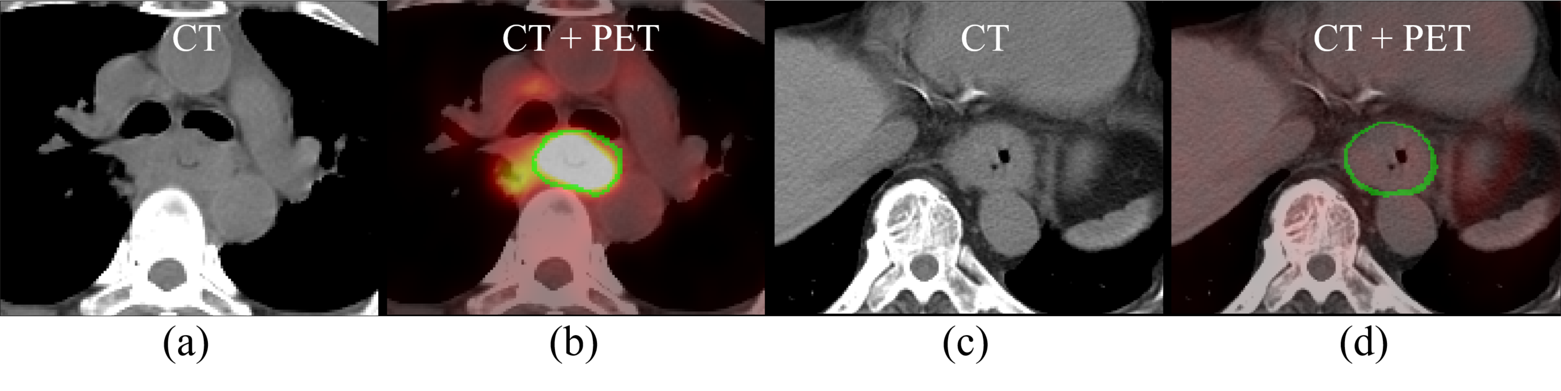
Figure 1: Esophageal GTV examples in CT and PET images, where the green line indicates the GTV boundary. (a)-(b): although the GTV boundaries are hardly distinguishable in CT, it can be reasonably inferred with the help of the PET image, in spite of other false positive high-uptake regions. (c)-(d) here, no high uptake regions appear in PET; however, the esophagus wall enlargement evident in CT may indicate the GTV boundary [6].

To address this gap, we propose a new approach, depicted in Fig. 2, that uses a two-stream chained pipeline to incorporate the joint RTCT and PET information for accurate esophageal GTV segmentation. First, we manage the misalignment between the RTCT and PET/CT by registering them via an anatomy-based initialization. Next, we introduce a two-stream chained pipeline that combines and merges predictions from two independent sub-networks, one only trained using the RTCT and one trained using both RTCT and registered PET images. The former exploits the anatomical contextual information in CT, while the latter takes advantage of PET’s sensitive, but sometimes spurious and overpoweringly strong contrast. The predictions of these two streams are then deeply fused together with the original RTCT to provide a final robust GTV prediction. Furthermore, we introduce a simple yet surprisingly powerful PSNN model, which incorporates the strengths of both UNet [2] and P-HNN [3] by using deep supervision to progressively propagate high-level semantic features to lower-level, but higher resolution features. Using 5-fold cross-validation, we evaluate the proposed approach on $110$ patients with RTCT and PET, which is more than two times larger than the previously largest reported dataset for esophageal GTV segmentation [15]. Experiments demonstrate that both our two-stream chained pipeline and the PSNN each provide significant performance improvements, resulting in an average DSC of $76.4\%\pm 13.4\%$, which is $11\%$ higher over the previous state-of-the-art method using DenseUNet [15].

2 Methods

Fig. 2 depicts an overview of our proposed two-stream chained esophageal GTV segmentation pipeline, which uses early and late 3D deep network fusions of CT and PET scans. Not shown is the registration step, which is detailed in §2.1.

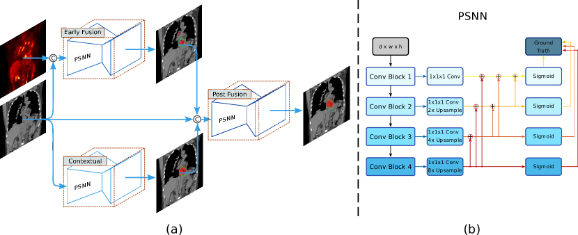
Figure 2: (a) depicts our two-stream chained esophageal GTV segmentation method consisting of EF and LF networks, while (b) illustrates the PSNN model, which employs deep supervision at different scales within a parameter-less high-to-low level image segmentation decoder. The first two and last two blocks are composed of two and three $3\times 3\times 3$ convolutional+BN+ReLU layers, respectively.

2.1 PET to RTCT Registration

To generate aligned PET/RTCT pairs, we register the former to the latter. This is made possible by the diagnostic CT accompanying the PET. To do this, we apply the cubic B-spline based deformable registration algorithm in a coarse to fine multi-scale deformation process [13]. We choose this option due to its good capacity for shape modeling and efficiency in capturing local non-rigid motions. However, to perform well, the registration algorithm must have a robust rigid initialization to manage patient pose and respiratory differences in the two CT scans. To accomplish this, we use the lung mass centers from the two CT scans as the initial matching positions. We compute mass centers from masks produced by the P-HNN model [3], which can robustly segment the lung field even in severely pathological cases. This leads to a reliable initial matching for the chest and upper abdominal regions, helping the success of the registration. The resulting deformation field is then applied to the diagnostic PET to align it to the RTCT at the planning stage. One registration example is illustrated in Fig. 3.

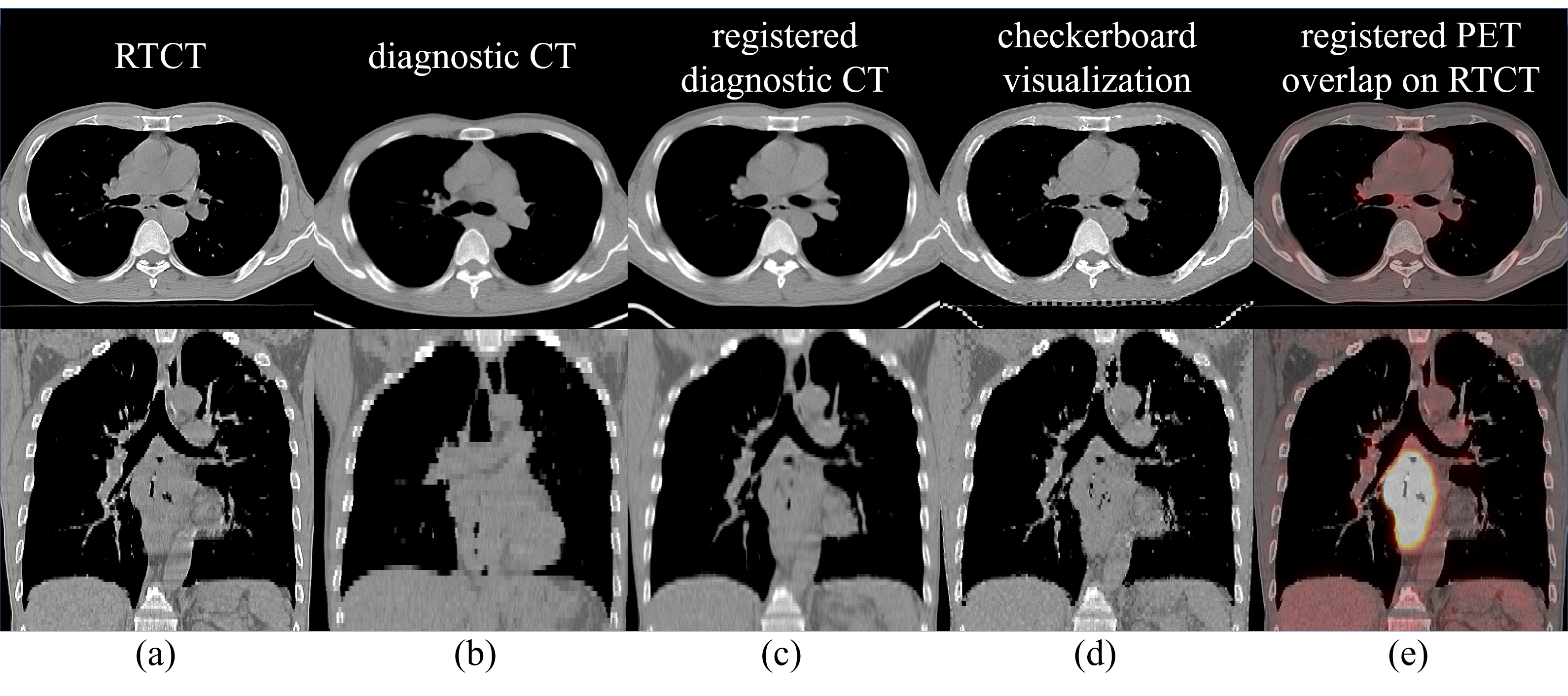
Figure 3: Deformable registration results for a patient shown in axial and coronal views. (a) shows the RTCT image; (b, c) depicts the diagnostic CT image before and after the registration, respectively; (d) depicts a checkerboard visualization of the RTCT and registered diagnostic CT images; and (e) overlays the PET image, transformed using the diagnostic CT deformation field, on top of the RTCT.

2.2 Two-Stream Chained Deep Fusion

As mentioned, we aim to effectively exploit the complementary information within the PET and CT imaging spaces. To do this, we design a two-stream chained 3D deep network fusion pipeline. Assuming $N$ data instances, we denote the training data as $S=\left\{\left(X^{\mathrm{CT}}_{n},X^{\mathrm{PET}}_{n},Y_{n}\right)\right\}_{n=1}^{N}$, where $X^{\mathrm{CT}}_{n}$, $X^{\mathrm{PET}}_{n}$, and $Y_{n}$ represent the input CT, registered PET, and binary ground truth GTV segmentation images, respectively. For simplicity and consistency, the same 3D segmentation backbone network (described in Sec. 2.3) is adopted. Dropping $n$ for clarity, we first use two separate streams to generate segmentation maps using $X^{\mathrm{CT}}$ and [$X^{\mathrm{CT}}$, $X^{\mathrm{PET}}$] as network input channels:

$$\hat{y}^{\mathrm{CT}}_{j} =p_{j}^{\mathrm{CT}}\left(y_{j}=1|X^{\mathrm{CT}};\mathbf{W}^{\mathrm{CT}}\right)\mathrm{,}$$ (1)

$$\hat{y}^{\mathrm{EF}}_{j} =p_{j}^{\mathrm{EF}}\left(y_{j}=1|X^{\mathrm{CT}},X^{\mathrm{PET}};\mathbf{W}^{\mathrm{EF}}\right)\mathrm{,}$$ (2)

where $p_{j}^{(\cdot)}(\cdot)$ and $\hat{y}^{(\cdot)}_{j}$ denote the CNN functions and output segmentation maps, respectively, $\mathbf{W}^{(\cdot)}$ represents the corresponding CNN parameters, and $y_{j}$ indicates the ground truth GTV tumor mask values. We denote Eq. (2) as EF, as the stream can be seen as an EF of CT and PET, enjoying the high spatial resolution and high tumor-intake contrast properties from the CT and PET, respectively. On the other hand, the stream in Eq. (1) provides predictions based on CT intensity alone, which can be particularly helpful in circumventing the biased influence from noisy non-malignant high uptake regions, which are not uncommon in PET.

As Fig. 2(a) illustrates, we harmonize the outputs from Eq. (1) and Eq. (2) by concatenating them together with the original RTCT image as the inputs to a third network:

$$\hat{y}^{\mathrm{LF}}_{j}=p_{j}^{\mathrm{LF}}\left(y_{j}=1|X^{\mathrm{CT}},\hat{Y}^{\mathrm{CT}},\hat{Y}^{\mathrm{EF}};\mathbf{W}^{\mathrm{CT}},\mathbf{W}^{\mathrm{EF}},\mathbf{W}^{\mathrm{LF}}\right)\mathrm{.}$$ (3)

In this way, the formulation of Eq. (3) can be seen as a LF of the aforementioned two streams of the CT and EF models. We use the DSC loss for all three sub-networks, training each in isolation.

2.3 PSNN Model

In esophageal GTV segmentation, the GTV target region often exhibits low contrast in CT, and the physician’s manual delineation relies heavily upon high-level semantic information to disambiguate boundaries. In certain respects, this aligns with the intuition behind UNet, which decodes high-level features into lower-level space. Nonetheless, the decoding path in UNet consumes a great deal of parameters, adding to its complexity. On the other hand, models like P-HNN [3] use deep supervision to connect lower and higher-level features together using parameter-less pathways. However, unlike UNet, P-HNN propagates lower-level features down to high-level layers. Instead, a natural and simple means to combine the strengths of both P-HNN and UNet is to use essentially the same parameter blocks as P-HNN, but reverse the direction of the deeply-supervised pathways, to allow high-level information to propagate up to lower-level space. We denote such an approach as PSNN.

As shown in Fig. 2(b), a set of $1\times 1\times 1$ 3D convolutional layers are used to collapse the feature map after each convolutional block into a logit image, i.e., $\tilde{f}_{j}^{(\ell)}$, where $j$ indexes the pixel locations. This is then combined with the previous higher level segmentation logit image to create an aggregated segmentation map, i.e., $f_{j}^{(\ell)}$, for the $\ell^{th}$ feature block by element-wise summation:

$$f_{j}^{(m)} =\tilde{f}_{j}^{(m)}\textrm{,}$$ (4)

$$f_{j}^{(\ell)} =\tilde{f}_{j}^{(\ell)}+g\left(f_{j}^{(\ell+1)}\right),\forall\ell\in\{m-1,\cdots,1\},$$ (5)

where $m$ denotes the total number of predicted feature maps and $g(\cdot)$. denotes an upsampling, i.e., bilinear upsampling. The PSNN model is trained using four deeply-supervised auxiliary losses at each convolutional block. As our experiments will demonstrate, PSNN can provide significant performance gains for GTV segmentation over both a densely connected version of UNet [15] and P-HNN [3].

3 Experiments and Results

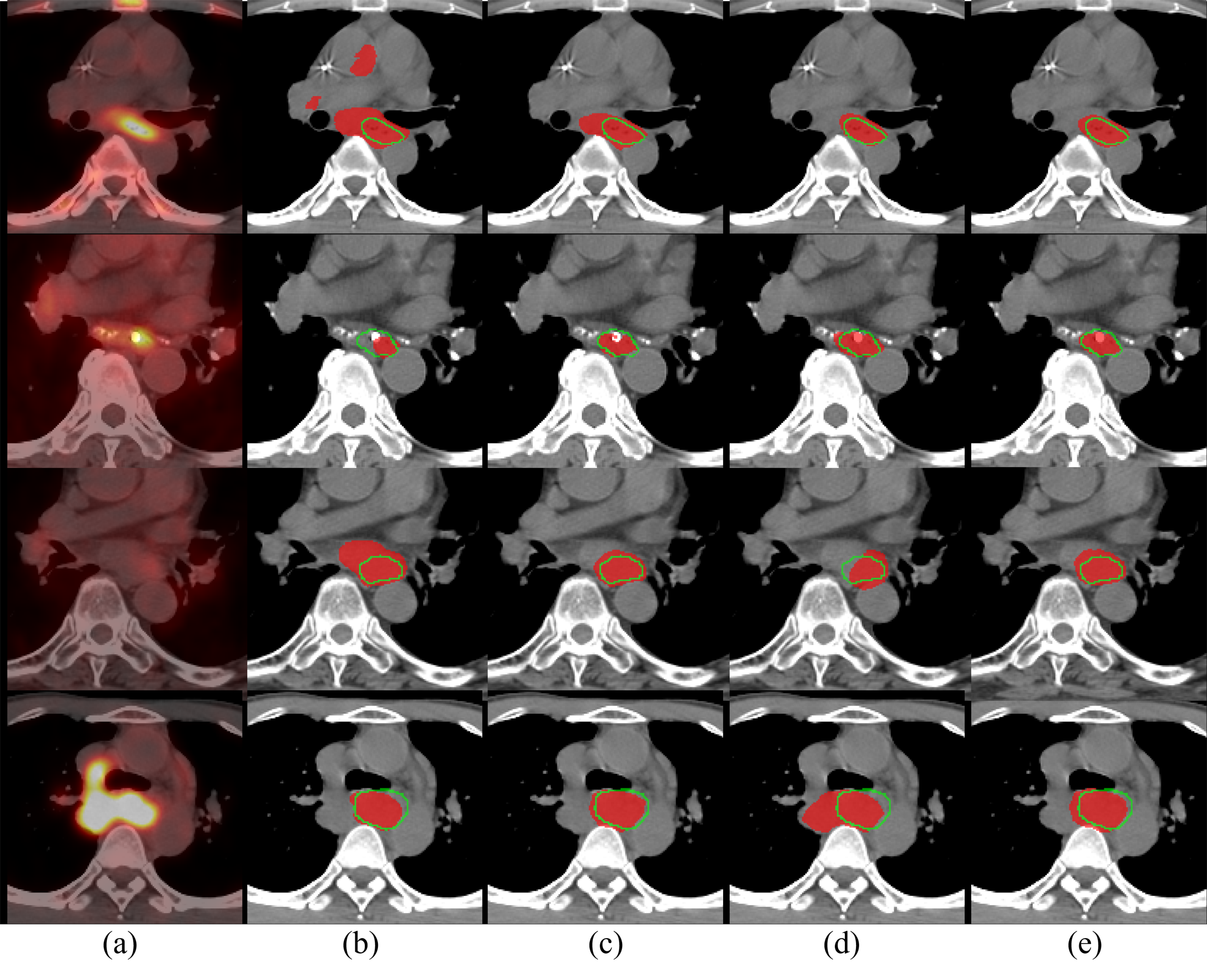
Figure 4: Qualitative results of esophageal GTV segmentation. (a) RTCT overlayed with the registered PET channel; (b) GTV segmentation results using RTCT images with DenseUNet [15]; (c) Our results using Eq. (1), i.e., RTCT-only stream using the proposed PSNN model; (d) Our results using Eq. (2) with PSNN, i.e., EF of PET+RTCT images; (e) Our final GTV segmentation using Eq. (3) with PSNN, i.e., EF and LF of PET+RTCT images. Red masks indicate automated segmentation results and green boundaries represent the ground truth. The first two rows demonstrate the importance of PET as using RTCT alone can cause under- or over-segmentation due to low contrast. The last two rows show cases where under- or over-segmentation can occur when the PET imaging channel is spuriously noisy. In all cases, the final EF+LF based GTV segmentation results achieve good accuracy and robustness.

We extensively evaluate our approach using a dataset of $110$ esophageal cancer patients, all diagnosed at stage II or later and undergoing RT treatments. Each patient has a diagnostic PET/CT pair and a treatment RTCT scan. To the best of our knowledge, this is the largest dataset collected for esophageal cancer GTV segmentation. All 3D GTV ground truth masks are delineated by two experienced radiation oncologists during routine clinical workflow. We first resample all imaging scans of registered PET and RTCT to a fixed resolution of $1.0\times 1.0\times 2.5$ mm. To generate positive training instances, we randomly sample $80\times 80\times 64$ sub-volumes centered inside the ground truth GTV mask. Negative examples are extracted by randomly sampling from the whole 3D volume. This results, on average, in $80$ training sub-volumes per patient. We further apply random rotations in the x-y plane within $\pm 10$ degrees to augment the training data.

Table 1: Mean DSCs, HDs, and $\text{ASD}_{GT}$, and their standard deviations of GTV segmentation performance using: (1) Contextual model using only CT images (CT); (2) Early fusion model (EF) using both CT and PET images; (3) The proposed two-stream chained early and late fusion model (EF+LF). 3D DenseUNet model using CT is equivalent to the previous state-of-the-art work [15], which is shown in the first row. The best performance scores are shown in bold.

	CT	EF	EF+LF	DSC	HD (mm)	$\text{ASD}_{GT}$ (mm)
3D DenseUNet	✓			0.654$\pm$0.210	129.0$\pm$73.0	5.2$\pm$12.8
		✓		0.710$\pm$0.189	116.0$\pm$81.7	4.9$\pm$10.3
			✓	0.745$\pm$0.163	79.5$\pm$70.9	4.7$\pm$10.5
3D P-HNN	✓			0.710$\pm$0.189	86.2$\pm$67.4	4.3$\pm$5.3
		✓		0.735$\pm$0.158	57.9$\pm$61.1	3.6$\pm$3.7
			✓	0.755$\pm$0.148	47.2$\pm$52.3	3.8$\pm$4.8
3D PSNN	✓			0.728$\pm$0.158	66.9$\pm$59.2	4.2$\pm$5.4
		✓		0.758$\pm$0.136	67.0$\pm$59.1	3.2$\pm$3.1
			✓	0.764$\pm$0.134	47.1$\pm$56.0	3.2$\pm$3.3

Implementation details: The Adam solver [10] is used to optimize all the 3D segmentation models with a momentum of $0.99$ and a weight decay of $0.005$ for $40$ epochs. For testing, we use 3D sliding windows with sub-volumes of $80\times 80\times 64$ and strides of $48\times 48\times 32$ voxels. The probability maps of sub-volumes are aggregated to obtain the whole volume prediction.

We employ five-fold cross-validation protocol split at the patient level. Extensive comparisons of our PSNN model versus P-HNN [3] and DenseUNet [15] methods are reported, with the latter arguably representing the current state-of-the-art GTV segmentation approach using CT. Three quantitative metrics are utilized to evaluate the GTV segmentation performance: DSC, HD in “mm”, and ASD in “mm”.

Results: Our quantitative results and comparisons are tabulated in Table 1. When all models are trained and evaluated using only RTCT, i.e., Eq. (1), our proposed PSNN evidently outperforms the previous best esophageal GTV segmentation method, i.e., DenseUNet [15], which straightforwardly combines DenseNet [5] and 3D UNet [2]. As can be seen, PSNN consistently improves upon [15] in all metrics: with an absolute increase of $7.4\%$ in DSC (from $0.654$ to $0.728$) and significantly dropping in HD metric, despite being a simpler architecture. PSNN also outperforms the 3D version of P-HNN [3], which indicates that the semantically-nested high- to low-level information flow provides key performance increases.

Table 1 also outlines the performances of three deep models under different imaging configurations. Several conclusions can be drawn. First, all three networks trained using the EF of Eq. (2) consistently produce more accurate segmentation results than those trained with only RTCT, i.e., Eq. (1). This validates the effectiveness of utilizing PET to complement RTCT for GTV segmentation. Second, the full two-stream chained fusion pipeline of Eq. (3) provides further performance improvements. Importantly, the performance boosts can be observed across all three deep CNN, validating that the two-stream combination of EF and LF can universally improve upon different backbone segmentation models. Last, the best performing results are the PSNN model combined with chained EF+LF, demonstrating that each component of the system contributes to our final performance. When compared to the previous state-of-the-art work of GTV segmentation, which uses DenseUNet applied to RTCT images [15], our best performing model exceeds in all metrics of DSC, HD, and ASD by $11\%$, $81.9mm$ and $2.0mm$ remarked margins (refer to Table 1), representing tangible and significant improvements. Fig. 4 shows several qualitative examples visually underscoring the improvements that our two-stage PSNN approach provides.

4 Conclusion

This work has presented and validated a two-stream chained 3D deep network fusion pipeline to segment esophageal GTV using both RTCT and PET+RTCT imaging channels. Diagnostic PET and RTCT are first longitudinally registered using semantically-based lung-mass center initialization to achieve robustness. We next employ the PSNN model as a new 3D segmentation architecture, which uses a simple, parameter-less, and deeply-supervised CNN decoding stream. The PSNN model is then used in a cascaded EF and LF scheme to segment the GTV. Extensive tests on the largest esophageal dataset to date demonstrate that our PSNN model can outperform the state-of-the-art P-HNN and DenseUNet networks with remarked margins. Additionally, we show that our 2-stream chained fusion pipeline produces further important improvements, providing an effective means to exploit the complementary information seen within PET and CT. Thus, our work represents a step forward toward accurate and automated esophageal GTV segmentation.

References

- [1] Bray, F., Ferlay, J., et al.: Global cancer statistics 2018: Globocan estimates of incidence and mortality worldwide for 36 cancers in 185 countries. CA: a cancer journal for clinicians 68(6), 394–424 (2018)
- [2] Çiçek, Ö., Abdulkadir, A., Lienkamp, S.S., et al.: 3d u-net: Learning dense volumetric segmentation from sparse annotation. In: MICCAI. pp. 424–432 (2016)
- [3] Harrison, A.P., Xu, Z., George, K., et al.: Progressive and multi-path holistically nested neural networks for pathological lung segmentation from ct images. In: MICCAI. pp. 621–629. Springer (2017)
- [4] Holger, R., Lu, L., Lay, N., et al.: Spatial aggregation of holistically-nested convolutional neural networks for automated pancreas localization and segmentation. Medical Image Analysis 45, 94–107 (2018)
- [5] Huang, G., Liu, Z., van der Maaten, L., Weinberger, K.Q.: Densely connected convolutional networks. In: IEEE CVPR. pp. 2261–2269 (2017)
- [6] Iyer, R., Dubrow, R.: Imaging of esophageal cancer. Cancer Imaging 4(2), 125 (2004)
- [7] Jin, D., Guo, D., Ho, T.Y., et al.: Deep esophageal clinical target volume delineation using encoded 3d spatial context of tumor, lymph nodes, and organs at risk. In: MICCAI. Springer (2019)
- [8] Jin, D., Xu, Z., Harrison, A.P., et al.: 3d convolutional neural networks with graph refinement for airway segmentation using incomplete data labels. In: Machine Learning in Medical Imaging. pp. 141–149. Springer (2017)
- [9] Jin, D., Xu, Z., Tang, Y., et al. J: Ct-realistic lung nodule simulation from 3d conditional generative adversarial networks for robust lung segmentation. In: MICCAI. pp. 732–740. Springer (2018)
- [10] Kingma, D.P., Ba, J.: Adam: A method for stochastic optimization. arXiv:1412.6980 (2014)
- [11] Leong, T., Everitt, C., et al.: A prospective study to evaluate the impact of fdg-pet on ct-based radiotherapy treatment planning for oesophageal cancer. Radiotherapy and oncology 78(3), 254–261 (2006)
- [12] Muijs, C., Schreurs, L., et al.: Consequences of additional use of pet information for target volume delineation and radiotherapy dose distribution for esophageal cancer. Radiotherapy and Oncology 93(3), 447–453 (2009)
- [13] Rueckert, D., Sonoda, L.I., Hayes, C., et al. J: Nonrigid registration using free-form deformations: application to breast mr images. IEEE TMI 18(8), 712–721 (1999)
- [14] Tai, P., Van Dyk, J., Yu, E., et al.: Variability of target volume delineation in cervical esophageal cancer. Int. J. of Radiation Oncology Biology Physics 42(2), 277–288 (1998)
- [15] Yousefi, S., Sokooti, H., et al.: Esophageal gross tumor volume segmentation using a 3d convolutional neural network. In: MICCAI. pp. 343–351. Springer (2018)
- [16] Zhao, H., Liu, J., Liu, J.: Esophagus tumor segmentation using fully convolutional neural network and graph cut. In: Intelligent Systems. pp. 413–420. Springer (2017)
- [17] Zhao, X., Li, L., et al.: Tumor co-segmentation in pet/ct using multi-modality fully convolutional neural network. Physics in Medicine & Biology 64(1), 015011 (2019)
- [18] Zhong, Z., Kim, Y., et al.: Simultaneous cosegmentation of tumors in pet-ct images using deep fully convolutional networks. Medical physics 46(2), 619–633 (2019)