Quantum walks of a phonon in trapped ions

Abstract

Propagation and interference of quantum-mechanical particles comprise an important part of elementary processes in quantum physics, and their essence can be modeled using a quantum walk, a mathematical concept that describes the motion of a quantum-mechanical particle among discretized spatial regions. Here we report the observation of the quantum walks of a phonon, a vibrational quantum, in a trapped-ion crystal. By employing the capability of preparing and observing a localized wave packet of a phonon, the propagation of a single radial local phonon in a four-ion linear crystal is observed with single-site resolution. The results show an agreement with numerical calculations, indicating the predictability and reproducibility of the phonon system. These characteristics may contribute advantageously in advanced experimental studies of quantum walks with large numbers of nodes, as well as realization of boson sampling and quantum simulation using phonons as computational resources.

I Introduction

Propagation of quantum-mechanical particles in media is essential to various fields including quantum optics, condensed-matter physics and quantum information science. Recent experimental progress has enabled observing the propagation of individual quanta, and this is discussed in the context of quantum walks (QWs) Aharonov et al. (1993); Venegas-Andraca (2012). QWs can be extended to multiple walkers Peruzzo et al. (2010), and are used to model universal computation Childs (2009); Childs et al. (2013). So far photons have been a major platform for realizing QWs Bouwmeester et al. (2000); Perets et al. (2008); Peruzzo et al. (2010). There have been also realizations with neutral atoms Preiss et al. (2015) and trapped ions Schmitz et al. (2009); Zähringer et al. (2010). More recently, QWs of one and two correlated microwave photons have been demonstrated with a superconducting system Yan et al. (2019).

Local phonons (quanta of local vibrational motions) in the trapped ions Porras and Cirac (2004) show particle-like characteristics and undergo interference via beamsplitter-like coupling due to inter-ion Coulomb interactions Porras and Cirac (2004); Brown et al. (2011); Harlander et al. (2011); Haze et al. (2012); Toyoda et al. (2015), thereby acting in a similar way to photons. Phonons in trapped ions has the merit of being generated and detected in deterministic ways. Optical manipulation of phonons and incorporating interaction among them are possible Debnath et al. (2018); Ivanov et al. (2009); Toyoda et al. (2013); Ding et al. (2017a, b). These characteristics can be utilized in realization of QWs as well as boson sampling Shen et al. (2014) and the Jaynes-Cummings-Hubbard model Ivanov et al. (2009); Toyoda et al. (2013).

Propagation of local phonons so far has been observed with axial motions of two ions in double-well potentials or radial motions of a two-ion linear crystal Brown et al. (2011); Harlander et al. (2011); Haze et al. (2012), and in a three-ion linear crystal where blockade of hopping using site-dependent AC Stark shifts is realized Debnath et al. (2018). In Ramm et al. (2014); Abdelrahman et al. (2017), energy transport is studied with radial motional modes in chains of up to 42 trapped ions which are cooled to thermal states using Doppler cooling.

In this article, we present results on the propagation of a local phonon among four sites of an ion crystal. The radial motion of the ion crystal is cooled to near the ground state, and one phonon is prepared at a desired site with an individual optical access, whose propagation over the ion crystal is traced by a site-resolved observation. The phonon freely propagate among the four ion sites, showing the high-contrast patterns of complex wave-packet interference for up to 10 ms, which corresponds to $\sim$60 times the maximum adjacent-hopping time (the maximum time required for a phonon to move between adjacent two sites). The interference patterns are compared with numerically calculated results, showing agreements in detail. The experimental results are also analyzed in the frequency domain, showing agreements with theoretical predictions based on radial collective-mode analyses.

The phonon propagation observed here, which is interpreted as a continuous-time QW Farhi and Gutmann (1998) of a local-phonon wave packet, can be extended in a straightforward manner to larger numbers of ion sites, and hence the investigation of continuous-time QWs in larger systems may become possible. Extension with regard to the number of phonons is also possible, allowing the realization of boson sampling for the demonstration of quantum computing power that may overwhelm the state-of-the-art classical computing Aaronson and Arkhipov (2011); Shen et al. (2014).

II Results

II.1 QWs of a phonon

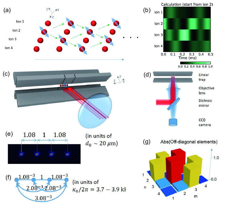
Figure 1: QWs of a phonon. (a) Conceptual diagram for the QW of a phonon. First a phonon (radial local phonon oscillating in the $y$ direction) is prepared in the ion 2. Due to the Coulomb coupling, it split into two wave packets and propagates to either the ion 1 or 3. The ion 1 is at the edge of the crystal, and hence the the phonon wave packet is reflected back there, propagating again to the ion 2, where it interferes with another wave packet coming from the ion 3. In this way the complex pattern of propagation and interference is formed. (b) Numerically calculated result for the QW of a phonon. A phonon is prepared in the ion 2, from which it propagates and interfere with itself as described above. Conditions similar to what is used in the experiment are assumed in this calculation. (c) Setup for the optical excitation of the ions to generate and observe a phonon. A linear Paul trap used, four ions trapped inside it, optical beams for excitation and an objective lens are depicted. (d) Schematic for the setup of optical excitation and fluorescence observation. (e) Ion string used. The distances between adjacent pairs of ions are described. (f) Graph structure when the phonon propagation is viewed as a continuous-time QW. The values are hopping rates corresponding to each edges in units of $\kappa_{0}/2\pi$ (hopping rates between the central two ions). (g) Absolute values of the Hamiltonian off-diagonal elements for phonon propagation.

Figure 1 shows the concepts, configurations and conditions for the experiment on the QWs of a phonon. Figure 1(a) shows the conceptual diagram for the QWs of a phonon in a linear crystal of four ions (numbered as 1-4). First a phonon (radial local phonon oscillating in the $y$ direction) is prepared in the ion 2. Due to the inter-mode coupling arising from the Coulomb interaction between ions, the phonon split into two wave packets and propagates to either the ion 1 or 3. Since the ion 1 is at the edge of the crystal, the phonon wave packet that has proceeded there gets reflected and propagates back to the ion 2, where it interferes with another wave packet coming from the ion 3. In this way a complex pattern of propagation and interference is formed. A numerically calculated result showing a similar behavior is given in Fig. 1(b). Conditions similar to what is used in the experiment are assumed in this calculation. The ions are illuminated with four independent beams [Fig. 1(c)], and fluorescence from all ions is imaged onto an electron multiplying charge-coupled device [Fig. 1(d)]. Figure 1(e) shows the ion string used, where the distances between adjacent pairs of ions are described. Figure 1(f) shows the graph structure when the phonon propagation is viewed as a continuous-time QW. The values are the hopping rates corresponding to each edges in units of $\kappa_{0}$ (hopping rates between central two ions). The corresponding Hamiltonian off-diagonal elements (see Materials and Methods) are plotted in Fig. 1(g).

II.2 Results in the time domain

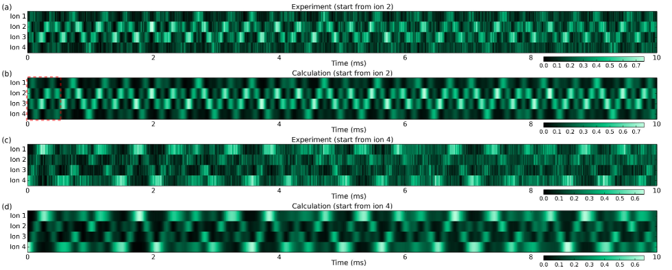
Figure 2: Results for phonon propagation in the time domain. The experimental and numerically calculated results for the time dependence of the local-phonon existence probability after one phonon is prepared at a particular site are displayed as brightness. (a) [(c)] Experimental result with the initial phonon population at the ion 2 [4]. Each of the four rows represent the time dependence of the local-phonon existence probability at each ion site, from the ion 1 (top) to 4 (bottom). The width of each time step is 12.5 $\mu$s, and the number of measurements per step is 50. (b) [(d)] Numerically calculated result with the initial phonon population at the ion 2 [4]. The area surrounded by the thin-red dashed rectangular at the left end in (b) corresponds to that displayed in Fig. 1(b).

Figure 2(a) (2(c)) shows the experimental result for the phonon propagation with the initial phonon population at the ion 2 (4). The phonon prepared at the ion 2 (4) splits and propagates among the four ion sites. Figure 2(b) (2(d)) shows the numerical result with the initial phonon population at the ion 2 (4) calculated using the Hamiltonian of Eq. 2 in Materials and Methods. For obtaining these calculated results, the following four parameters are adjusted so as to minimize the residual sum of squares: the horizontal time scale (determined by $\kappa_{0}\propto\omega_{z}^{2}/\omega_{y}$ where $\omega_{z}$ and $\omega_{y}$ are the oscillation frequencies for the axial $z$ and radial $y$ directions, respectively), the horizontal offset (due to the fact that hopping may occur during the preparation time), the population scale factors (explained below), and the heating rate ($\sim$5 quanta per second). The population scale factors are the overall proportionality factors multiplied to the calculated results. We need to adjust those factors because of the reduction of preparation and observation efficiency due to the decoherence in applying the red-sideband $\pi$ pulses. Their explicit values are 0.66 and 0.76 for the initial phonon population at the ion 2 and 4, respectively. Each calculated result shows an agreement with the corresponding experimental result up to the propagation time of 10 ms.

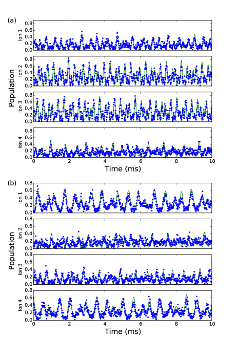
Figure 3: Two-dimensional plots of the results for phonon propagation in the time domain. The same experimental and numerically calculated results as shown in Fig. 2) are displayed using two-dimensional plots. (a) [(b)] Result with the initial phonon population at the ion 2 [4]. Each of the four rows represent the time dependence of the local-phonon existence probability at each ion site, from the ion 1 (top) to 4 (bottom). The points represent the experimental data points, and the curves represent the numerically calculated results. For the experimental data points, the width of each time step is 12.5 $\mu$s, and the number of measurements per step is 50.

Figure 3 shows the experimental and numerically calculated results in the time domain (the same results as shown in Fig. 2) displayed using two-dimensional plots. Figure 3(a) (3(b)) shows the result with the initial phonon population at the ion 2 (4). Each of the four rows represent the time dependence of the local-phonon existence probability at each ion site, from the ion 1 (top) to 4 (bottom). The points represent the experimental data points, and the curves represent the numerically calculated results (obtained by adjusting the parameters to minimize the residual sum of squares, as described above).

II.3 Results in the frequency domain

Since the local phonon can be interpreted as a superposition of collective-mode phonons, the behavior of phonon propagation in the time domain can be understood as a wave interference among different collective modes. From this view point, it is expected that the Fourier transforms of the time-domain results give information about the collective modes involved, thereby enabling the analyses of the phonon propagation in the frequency domain. Below we describe the formalism useful for such analyses.

By diagonalizing the potential and Coulomb-energy parts of the radial-motion Hamiltonian with the harmonic approximation, eigenvalues $\omega_{p}$ and real-valued eigenvectors $b_{n}^{(p)}$ can be obtained Zhu et al. (2006), where $p$ and $n$ are the indices for the radial collective modes and ions, respectively. The Heisenberg-picture local-phonon annihilation operator at the ion $n$ can be represented as follows using $b_{n}^{(p)}$ and the collective-mode annihilation operator $\hat{c}_{p}$: $\hat{a}_{n}(t)=\sum_{p}{}b_{n}^{(p)}\hat{c}_{p}{}e^{-i\omega_{p}{}t}$. The initial state with one phonon at the ion $n$ is $\ket{\Phi_{n}}=\hat{a}_{n}^{\dagger}(0)\ket{\Phi_{0}}=(\sum_{p}{}b_{n}^{(p)}\hat{c}_{p}^{\dagger})\ket{\Phi_{0}}$, where $\ket{\Phi_{0}}=\ket{0,0,\cdots,0}$ is the ground state of the collective-mode Fock states. Using these, the probability for one phonon (prepared at time 0 and the ion $n$) observed at time $t$ and ion $m$ is obtained as follows:

$$P_{nm}\equiv\braket{\Phi_{n}}{\hat{a}_{m}^{\dagger}(t){}\hat{a}_{m}(t)}{\Phi_{n}}$$

$$=\sum_{p,q}b_{n}^{(q)}b_{m}^{(q)}e^{i\omega_{q}t}e^{-i\omega_{p}t}b_{m}^{(p)}b_{n}^{(p)}$$

$$=\sum_{p}\left(b_{n}^{(p)}b_{m}^{(p)}\right)^{2}+\sum_{q>p}b_{n}^{(q)}b_{m}^{(q)}b_{m}^{(p)}b_{n}^{(p)}\left[e^{i(\omega_{q}-\omega_{p})t}+\rm{c.c.}\right]$$

Therefore, the amplitude of the positive and negative frequency component oscillating at $\omega_{q}-\omega_{p}$ and $-(\omega_{q}-\omega_{p})$, respectively, is equal to $b_{n}^{(q)}b_{m}^{(q)}b_{m}^{(p)}b_{n}^{(p)}$ ($q>p$ and $\omega_{q}>\omega_{p}$ for $q>p$ assumed).

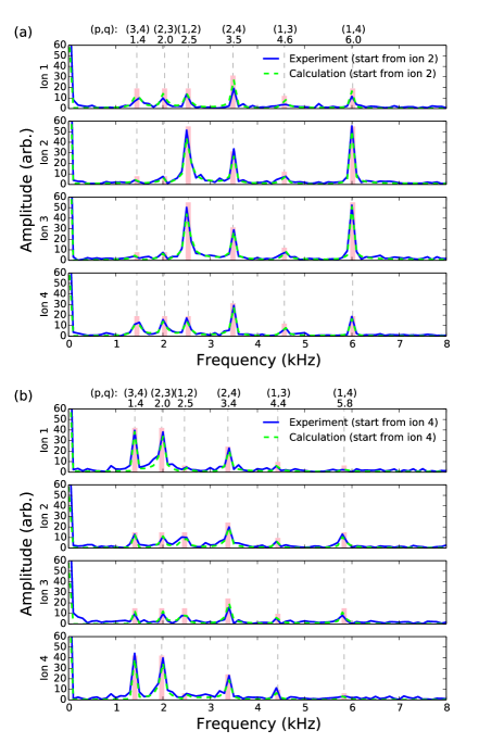
Figure 4: Results for phonon propagation in the frequency domain. (a) [(b)] Result with the initial phonon population at the ion 2 [4]. The Fourier transform of the local-phonon existence probability is plotted. The blue solid (green dashed) curves represent the experimental (numerically calculated) results. The light-red vertical bars represent analytically obtained results corresponding to $b_{n}^{(q)}b_{m}^{(q)}b_{m}^{(p)}b_{n}^{(p)}$ (see text). The vertical gray dashed lines represents the difference of frequencies ($\omega_{q}-\omega_{p}$) for each pairs of radial collective modes. The texts at the top represents the pairs of indices $(p,q)$ for the relevant collective-mode pairs, where the indices 1-4 are taken in the order of increasing oscillation frequencies. The texts in the second row from the top represents the difference of frequencies ($\omega_{q}-\omega_{p}$) in the unit of kHz.

In Fig. 4, the Fourier transforms of populations at the ion sites are shown. The solid blue curves are the discrete Fourier transforms of the experimental results, and the green dashed curves are those of the calculated results. The light-red vertical bars are the analytically obtained results $b_{n}^{(q)}b_{m}^{(q)}b_{m}^{(p)}b_{n}^{(p)}$ multiplied with appropriate proportionality factors for comparison with the discrete Fourier transforms. The vertical gray dashed lines represents the difference of frequencies ($\omega_{q}-\omega_{p}$) for each pairs of radial collective modes. It is understood from the plot that the three results match well with each other.

III Discussion

In conclusion, we have experimentally shown that a phonon in trapped ions undergoes propagation and interference that can be interpreted as a quantum walk. We have observed propagation dynamics for up to 10 ms, and the results has been compared with numerically calculated ones, showing agreements. It can be expected that the system of phonons offers a platform for realizing quantum walks in larger scales and non-universal quantum-computationa schemes including boson sampling.

The current experiment is performed with single phonon, while it has been pointed out that single particle (discrete) QWs are shown to be implementable with classical devices Knight et al. (2003a, b); Jeong et al. (2004); Venegas-Andraca (2012). The genuine quantum mechanical properties can be investigated with the use of multiple walkers. Extension to multiple phonons is also possible in the system of phonons in trapped ions. Preparation of multiple phonons in desired sites in a deterministic way is possible with standard techniques using sequences involving carrier and sideband transitions and site-resolved optical manipulation. The detection of multiple phonons (projection measurements) is also possible in principle, and has been performed with a single ion An et al. (2015).

The efficiency of the initial-state preparation and final-state measurement in our system is limited due to the infidelity in red-sideband $\pi$ pulses ($\sim$0.7-0.8 when combined). Since the present experiment is performed using a relatively weak axial confinement and tight focuses, the residual thermal fluctuation along the axial direction ($\sim$0.5 $\mu$m rms) is nonnegligible compared with the size of the focuses ($\sim$3 $\mu$m). Other possible factors of the decoherence might be the combinations of beam jitter, deteriorated spatial modes at the focus and AC Stark shifts Häffner et al. (2003).

Although heating is observed in the time span of up to 10 ms, the decoherence of phonon dynamics is not prominent in this time scale. Previously decay time of 13 ms, corresponding to $\sim$30 round trips in the case of two ions has been observed Toyoda et al. (2015), and this decay time seems to be dependent on certain experimental conditions, which include the radial/axial confinements, and the residual thermal motion along the axial direction, which is cooled only with Doppler cooling.

IV Materials and methods

IV.1 Phonon propagation as QWs

Propagation of a local phonon can be viewed as a QW. A QW is defined as a temporally homogeneous evolution of a quantum system defined on a graph comprising of vertices and edges. Two different formulations of QWs exist, namely in discrete time Aharonov et al. (1993) and continuous time Farhi and Gutmann (1998). It can be shown that local phonon propagation in trapped ions is equivalent to a continuous-time QW.

Continuous-time QWs are formulated using a generator matrix $M_{nm}$ ($\gamma$ is the jump rate and $k_{n}$ is the number of edges that are connected to vertex $n$): $M_{nm}=-\gamma_{nm}\ (n\neq{}m,n\mbox{ and }m\mbox{ connected by an edge});0\ (n\neq{}m,n\mbox{ and }m\mbox{ not connected});\sum_{l\neq{}n}\gamma_{nl}\ (n=m)$. The Hamiltonian $\hat{H}$ with matrix elements given by $\braket{n}{\hat{H}}{m}=M_{nm}$ ($\hbar{}=1$) generates an evolution described with the Schrödinger equation and the unitary evolution operator $U=\exp(-i\hat{H}t)$, which is interpreted as a QW in continuous time.

The Hamiltonian for a radial direction (denoted as the $y$ direction) in a linear ion crystal is described as follows Porras and Cirac (2004):

$$\hat{H}_{y}=\sum^{N}_{n=1}(\omega_{y}+\omega_{y,n})\hat{a}_{i}^{\dagger}\hat{a}_{n}-\sum^{N}_{m>n}t_{nm}(\hat{a}_{n}^{\dagger}\hat{a}_{m}+\hat{a}_{n}\hat{a}_{m}^{\dagger}).$$ (1)

Here $t_{nm}=-e^{2}/8\pi\epsilon_{0}m\omega_{y}|z_{n}^{0}-z_{m}^{0}|^{3}$ is the hopping amplitudes and $\omega_{y,n}=\sum^{N}_{m\neq{}n}t_{nm}$ is the harmonic correction terms for radial oscillation frequencies. If the rotating frame oscillating at $\omega_{y}$ is adopted and the case of only one phonon is considered ($\hat{a}_{n}^{\dagger}\hat{a}_{m}\rightarrow\ket{n}\bra{m}$), $\hat{H}_{y}=\sum^{N}_{n}(\sum_{m\neq{n}}t_{nm})\ket{n}\bra{n}-\sum_{m\neq{n}}t_{nm}\ket{n}\bra{m}$. By setting $\gamma_{nm}\equiv-t_{nm}$, this corresponds exactly to continuous-time QWs explained above.

IV.2 Experimental conditions

The experiment is performed with four ⁴⁰Ca⁺ ions (named as the ion 1-4) trapped in a three-dimensional linear Paul trap. The oscillation frequencies for the three directions $(x,y,z)$ are $(\omega_{x},\omega_{y},\omega_{z})/2\pi\sim(3.1,2.9,0.09)$ MHz, respectively. The distance of the central two ions ($d_{0}$) is $\sim 20$ $\mu$m. One of the radial directions referred to as $y$ is mainly used for the observation of phonon propagation. The radial-phonon hopping rate between the central two ions defined as $\kappa_{0}/2\pi=(e^{2}/4\pi\epsilon_{0}m\omega_{y}d_{0}^{3})/2\pi$ is 3.7 - 3.9 kHz. The heating rate for $y$ estimated from the propagation results is $\sim$5 quanta per second. Due to this heating, we limit the total measurement times up to 10 ms to make sure that only a single quantum of phonons exist in the system. The excess phonon population due to heating can be suppressed to below 5 % in this case.

In the condition given above, the explicit values for the Hamiltonian matrix elements are obtained as follows.

$$\frac{\kappa_{0}}{2}\left(\begin{array}[]{rrrr}-0.93&0.79&0.11&0.03\\ 0.79&-1.90&1.00&0.11\\ 0.11&1.00&-1.90&0.79\\ 0.03&0.11&0.79&-0.93\\ \end{array}\right)$$ (2)

The smallest matrix elements among the adjacent couplings in this Hamiltonian is $0.79\times\kappa_{0}/2$. This determines the maximum adjacent-hopping time, that is, the maximum time required for a phonon to hop to an adjacent site, which is obtained to be $(0.79\times\kappa_{0}/2\pi)^{-1}/2\sim 160$ $\mu$s. By using this, we can conclude that the total observation time used in this work (10 ms) corresponds to $\sim$60 times the maximum adjacent-hopping time.

The $S_{1/2}(m_{J}=-1/2)$–$D_{5/2}(m_{J}=-1/2)$ transition at 729 nm is used as the main transition for optical manipulation and observation of phonons. Each of four beams at 729 nm is focused onto each ion with the $1/e^{2}$ radius of $\sim$3 $\mu$m. The power for each beam is adjusted so that the Rabi frequency for every ion become equal to each other, which amounts to $\sim$400 kHz for the carrier transition and $\sim$16 kHz for the blue-sideband transition. This equal illumination is important for assuring equal efficiencies of preparation and mapping (explained in the next subsection) for all ions. Each of the four beams can be switched by using a dedicated acousto-optic modulator.

IV.3 Time sequence

First the ion crystal is Doppler cooled in all directions, and the radial two directions ($x$ and $y$) are cooled with sideband cooling to $\{\bar{n}_{x},\bar{n}_{y}\}\sim\{0.1,0.03\}$.

Then a blue-sideband and carrier $\pi$ pulses ($\sim$31 $\mu$s and $\sim$1.3 $\mu$s, respectively) are applied to a selected ion, which produce one radial local phonon. This is followed by a free evolution period with variable length, in which the generated phonon hops among the ion sites. After this, a mapping pulse (red-sideband $\pi$ pulse, $\sim$31 $\mu$s) is applied, which is followed by an internal state measurement using a 397-nm laser (resonant to the $S_{1/2}$–$P_{1/2}$ transition), whereby the two internal states $S_{1/2}$ and $D_{5/2}$ are discriminated.