Group Inference in High Dimensions with Applications to Hierarchical Testing

Summary

High-dimensional group inference is an essential part of statistical methods for analysing complex data sets, including hierarchical testing, tests of interaction, detection of heterogeneous treatment effects and inference for local heritability. Group inference in regression models can be measured with respect to a weighted quadratic functional of the regression sub-vector corresponding to the group. Asymptotically unbiased estimators of these weighted quadratic functionals are constructed and a novel procedure using these estimators for inference is proposed. We derive its asymptotic Gaussian distribution which enables the construction of asymptotically valid confidence intervals and tests which perform well in terms of length or power. The proposed test is computationally efficient even for a large group, statistically valid for any group size and achieving good power performance for testing large groups with many small regression coefficients. We apply the methodology to several interesting statistical problems and demonstrate its strength and usefulness on simulated and real data.

Key words: Heterogeneous Effects; Interaction Test; Local Heritability; Debiasing Lasso; Partial regression.

1 Introduction

1.1 Motivation and Formulation

Statistical inference for high-dimensional linear regression is an important but also challenging problem. This paper addresses a long-standing statistical problem, namely inference or testing significance of groups of covariates. Specifically, we consider the following high-dimensional linear regression

$$y_{i}=X_{i\cdot}^{\intercal}\beta+\epsilon_{i},\quad\text{for}\;i=1,\ldots,n,$$ (1)

where $X_{i\cdot}\in\mathbf{R}^{p}$ are independent and identically distributed random vectors with $\Sigma=\mathbf{E}X_{i\cdot}X_{i\cdot}^{\intercal}$ and $\epsilon_{i}$ are independent and identically distributed centred Gaussian errors, independent of $X_{i\cdot}$, with variance $\sigma^{2}$. For a given index set $G\subseteq\left\{1,2,\ldots,p\right\},$ we consider testing $H_{0}:\beta_{G}=0$ through testing the equivalent null hypothesis,

$${H}_{0,A}:\;\beta_{G}^{\intercal}A\beta_{G}=0,$$ (2)

where $A\in\mathbb{R}^{|G|\times|G|}$ is a positive-definite matrix with $|G|$ denoting the cardinality of $G$. The test (2) includes a class of tests for different $A$. By taking $A$ as $\Sigma_{G,G}$, (2) is specifically written as

$${H}_{0,\Sigma}:\;\beta_{G}^{\intercal}\Sigma_{G,G}\beta_{G}=0.$$ (3)

In addition, when $A$ is the identity matrix, (2) is reduced to ${H}_{0,{\rm I}}:\;\beta_{G}^{\intercal}\beta_{G}=0.$ The quantity $\beta_{G}^{\intercal}\Sigma_{G,G}\beta_{G}$ in (3) is naturally used for group significance testing as the quantity itself measures the variance explained by the set of variables $X_{i,G},$ $\beta_{G}^{\intercal}\Sigma_{G,G}\beta_{G}=\mathbf{E}|X_{i,G}^{\intercal}\beta_{G}|^{2}.$ The testing problem (3) can be conducted in both settings where the matrix $\Sigma_{G,G}$ is known or unknown. If $\Sigma_{G,G}$ is known, then it can be simply treated as a special case of (2). However, in the more practical setting with an unknown $\Sigma_{G,G}$, we need to estimate $\Sigma_{G,G}$ in the construction of the test statistic and quantify the additional uncertainty of estimating this matrix from data.

In the following, we shall provide a series of motivations for group inference or significance.

1. Hierarchical Testing. It is often too ambitious to detect significant single variables and groups of correlated variables are considered instead. Hierarchical testing is adjusting hierarchically over multiple group tests. It addresses the trade-off between signal strength and high correlation and it is a most natural way to deal with large-scale high-dimensional testing problems in real applications (Buzdugan et al.,, 2016; Klasen et al.,, 2016). More details are given in Section 4.1.

2. Interaction Test and Detection of Effect Heterogeneity. Group significance testing can be used to examine the existence of interaction. We write the model with interaction terms (Tian et al.,, 2014; Cai et al.,, 2019), $y_{i}=X_{i\cdot}^{\intercal}\beta+D_{i}\cdot X_{i\cdot}^{\intercal}\gamma+\epsilon_{i}$ for $i=1,\ldots,n$ with $D_{i}$ denoting the exposure variable and formulate the interaction test as $H_{0}:\gamma=0$. If $D_{i}$ denotes whether the $i$-th observation receives a treatment, then one can test against the presence of heterogenous treatment effects, see also Section 4.2.

3. Local Heritability in Genetics. Local heritability is among the most important heritability measures (Shi et al.,, 2016) and can be defined as $\mathbf{E}|X_{i,G}^{\intercal}\beta_{G}|^{2}=\beta_{G}^{\intercal}\Sigma_{G,G}\beta_{G}$ in (1), representing the proportion of variance explained by a subset of genotypes indexed by the group $G$. In applications, the group $G$ can be naturally formulated, e.g., the set of SNPs located on the same chromosome. It is of interest to test whether a group of genotypes with the index set $G$ is significant and construct confidence intervals for local heritability.

1.2 Results and Contribution

Statistical inference in high dimensional models has been studied in both statistics and econometrics with a focus on confidence interval and hypothesis testing for individual regression coefficients (Javanmard and Montanari,, 2014; van de Geer et al.,, 2014; Zhang and Zhang,, 2014; Chernozhukov et al.,, 2017; Cai and Guo,, 2017). Together with a careful use of bootstrap methods, certain maximum tests have been developed in Chernozhukov et al., (2017); Dezeure et al., (2017); Zhang and Cheng, (2017) to conduct the hypothesis testing problem $H_{0}:\beta_{G}=0$. These tests rely on the maximum of individual estimates and are tailored for sparse alternatives, and they can be computationally costly, especially when the size of $G$ is large. Instead of the maximum statistics which is favourable for sparse alternatives, we focus on sum-type statistics and also address the computational issue through directly testing the group significance. In low dimensions, the (partial) F-test is the classical sum-type procedure for testing group significance. However, there is a lack of sum-type methods for conducting group significance tests in high dimensions, especially for large groups. Our proposed group test with sum-type statistics can hence be viewed as an additional potentially powerful procedure in the toolkit of high-dimensional data analysis.

The proposed test statistic is constructed via an inference procedure for the quadratic form $\beta_{G}^{\intercal}A\beta_{G}$ in (3). We illustrate the main idea using ${\rm Q}_{\Sigma}=\beta_{G}^{\intercal}\Sigma_{G,G}\beta_{G}$ as an example. Denote by $\widehat{\beta}$ a reasonably good estimator (e.g. the Lasso estimator) of $\beta$ and define $\widehat{\Sigma}=\sum_{i=1}^{n}X_{i\cdot}X_{i\cdot}^{\intercal}/n$. The plug-in estimator $\widehat{\beta}^{\intercal}_{G}\widehat{\Sigma}_{G,G}\widehat{\beta}_{G}$ is not proper for statistical inference because it has a dominating bias inherited from $\widehat{\beta}.$ We correct the bias of this plug-in estimator through a novel projection. The proposed methodology can be extended to deal with the more general inference problem for $\beta_{G}^{\intercal}A\beta_{G}$ where $A\in\mathbb{R}^{|G|\times|G|}$ is a positive definite matrix.

The proposed test is valid for any group size $|G|$ in terms of type-I error control. As a generalization of the F-test to high-dimensions, the group tests proposed in Mitra and Zhang, (2016) and van de Geer and Stucky, (2016) require the group size $|G|$ to be smaller than the sample size. Our test has good power performance for testing large groups. The proposed test is asymptotically powerful as long as $\beta_{G}^{\intercal}\Sigma_{G,G}\beta_{G}$ is of a larger order of magnitude than $(1+\|\beta_{G}\|_{2}+\|\beta_{G}\|_{2}^{2})/n^{1/2}$. In comparison, the detection threshold of the $\chi^{2}$ test is in the order of $(|G|/n)^{1/2}$ (Mitra and Zhang,, 2016; van de Geer and Stucky,, 2016) which is inferior to the proposed test for a large $|G|.$ Additionally, for certain difficult settings, our proposed test achieves the same detection boundaries as the maximum test (Chernozhukov et al.,, 2017; Dezeure et al.,, 2017; Zhang and Cheng,, 2017), up to a constant, see the discussion after Corollary 2.

In Section 5, we compare the finite sample performance of the proposed sum-type test with the maximum test. In simulated data where the regression vector has many non-zero and small entries, we have observed that the proposed test has a better power performance; in simulated data with high correlation among covariates, the proposed confidence intervals achieve the desired coverage property while the coordinate-based inference procedures exhibit under-coverage.

Based on the proposed group test, a hierarchical testing algorithm inherits all of the above advantages in terms of both the computational efficiency and statistical validity. Even conceptually, hierarchical testing is fundamentally requiring a group test that is not based on the maximum of individual coordinates: the latter simply corresponds to a Bonferroni adjustment of individual coordinate tests and a hierarchical testing procedure would be useless. We illustrate some practical results in Sections 5.4 and 5.5.

1.3 Literature Comparison

In addition to the existing work based on the maximum test and generalization of $F$ tests mentioned above, there is other related work. Inference for the quadratic functionals is closely related to the group test. Statistical inference for $\beta^{\intercal}\Sigma\beta$ and $\|\beta\|_{2}^{2}$ has been carefully investigated in Verzelen and Gassiat, (2018); Cai and Guo, (2020); Guo et al., (2019) and the methods developed in Cai and Guo, (2020) have been extended to signal detection, which is a special case of (1) by setting $G=\{1,\ldots,p\}$. The group significance test problem is more challenging than signal detection, mainly due to the fact that the group test requires a decoupling between variables in $G$ and $G^{c}$. The decoupling between $G$ and $G^{c}$ essentially requires a novel construction of the projection direction. See Remark 2 in Section 2 for more details. The same comments can be made to differentiate the current paper with the signal detection problem considered in Ingster et al., (2010); Arias-Castro et al., (2011). Finally, Meinshausen, (2015) proposes another group significance test without any compatibility condition on the design. The price to be paid for this relaxation of conditions is in terms of a typically large drop in power.

2 Methodology for Testing Group Significance

We first present an inference procedure for ${\rm Q}_{\Sigma}=\beta_{G}^{\intercal}\Sigma_{G,G}\beta_{G}$ and will generalize it to inference for ${\rm Q}_{A}=\beta_{G}^{\intercal}A{\beta_{G}}.$ Throughout the paper, we use $\widehat{\beta}$ to denote a reasonably good estimator of $\beta$ and use $\widehat{\Sigma}=\sum_{i=1}^{n}X_{i\cdot}X_{i\cdot}^{\intercal}/n$ as the estimator of $\Sigma$. Without loss of generality, we assume the index set $G$ of the form $\{1,\ldots,|G|\}.$ To estimate ${\rm Q}_{\Sigma}$, we examine the error decomposition of a plug-in estimator $\widehat{\beta}_{G}^{\intercal}\widehat{\Sigma}_{G,G}\widehat{\beta}_{G}$ as $\widehat{\beta}_{G}^{\intercal}\widehat{\Sigma}_{G,G}\widehat{\beta}_{G}-\beta_{G}^{\intercal}\Sigma_{G,G}{\beta_{G}}=-2\widehat{\beta}_{G}^{\intercal}\widehat{\Sigma}_{G,G}(\beta_{G}-\widehat{\beta}_{G})+\beta_{G}^{\intercal}(\widehat{\Sigma}_{G,G}-\Sigma_{G,G})\beta_{G}-(\widehat{\beta}_{G}-\beta_{G})^{\intercal}\widehat{\Sigma}_{G,G}(\widehat{\beta}_{G}-\beta_{G}).$ In this decomposition, we need to estimate $2\widehat{\beta}_{G}^{\intercal}\widehat{\Sigma}_{G,G}(\beta_{G}-\widehat{\beta}_{G})$ as this is the dominant term to further calibrate the plug-in estimator $\widehat{\beta}_{G}^{\intercal}\widehat{\Sigma}_{G,G}\widehat{\beta}_{G}.$ The calibration can be done through identifying a projection direction $\widehat{u}\in\mathbb{R}^{p}$ to approximate $\widehat{\beta}_{G}^{\intercal}\widehat{\Sigma}_{G,G}(\beta_{G}-\widehat{\beta}_{G}).$ For any $u\in\mathbb{R}^{p},$

$$u^{\intercal}\frac{1}{n}X^{\intercal}(y-X\widehat{\beta})-\widehat{\beta}_{G}^{\intercal}\widehat{\Sigma}_{G,G}(\beta_{G}-\widehat{\beta}_{G})=\frac{1}{n}u^{\intercal}X^{\intercal}\epsilon+\left\{\widehat{\Sigma}u-(\widehat{\beta}_{G}^{\intercal}\widehat{\Sigma}_{G,G},{\bf 0})^{\intercal}\right\}^{\intercal}(\beta-\widehat{\beta}).$$

In this decomposition, $\frac{1}{n}u^{\intercal}X^{\intercal}\epsilon$ can be viewed as a variance component with asymptotically normal distribution; the second term on the right hand side can be controlled by Hölder inequality, $\Big{|}\Big{\{}\widehat{\Sigma}u-\big{(}\widehat{\beta}_{G}^{\intercal}\widehat{\Sigma}_{G,G},{\bf 0}\big{)}^{\intercal}\Big{\}}^{\intercal}(\beta-\widehat{\beta})\Big{|}\leq\|\beta-\widehat{\beta}\|_{1}\Big{\|}\widehat{\Sigma}u-(\widehat{\beta}_{G}^{\intercal}\widehat{\Sigma}_{G,G},{\bf 0})^{\intercal}\Big{\|}_{\infty}.$ As long as $\widehat{\beta}$ is a reasonable estimator with a small $\|\beta-\widehat{\beta}\|_{1},$ it remains to construct the projection direction $u\in\mathbb{R}^{p}$ such that $\big{\|}\widehat{\Sigma}u-(\widehat{\beta}_{G}^{\intercal}\widehat{\Sigma}_{G,G},{\bf 0})^{\intercal}\big{\|}_{\infty}$ is constrained. A direct generalization of “constraining bias and minimizing variance” in Javanmard and Montanari, (2014) leads to

$$\widetilde{u}=\arg\min\;u^{\intercal}\widehat{\Sigma}u\quad{\rm s.t.}\;\;\|\widehat{\Sigma}u-(\widehat{\beta}_{G}^{\intercal}\widehat{\Sigma}_{G,G},{\bf 0})^{\intercal}\|_{\infty}\leq\|\widehat{\Sigma}_{G,G}\widehat{\beta}_{G}\|_{2}\lambda_{n}$$ (4)

where $\lambda_{n}=C_{0}(\log p/n)^{1/2}$ for some constant $C_{0}>0.$ However, such a generalization does not always work: if $\|\widehat{\Sigma}_{G,G}\widehat{\beta}_{G}\|_{2}\lambda_{n}\geq\|\widehat{\Sigma}_{G,G}\widehat{\beta}_{G}\|_{\infty}$, we have $\widetilde{u}=0$ as the solution and do not conduct any bias correction. When $|G|$ is large and the elements of the vector $\widehat{\Sigma}_{G,G}\widehat{\beta}_{G}$ are of a similar order, then $\widetilde{u}=0$ as long as $\sqrt{|G|\log p/n}\geq C$ for some positive constant $C>0.$

To do the bias correction for arbitrary groups, we construct the projection direction $u$ as

$$\widehat{u}=\arg\min\;u^{\intercal}\widehat{\Sigma}u\quad{\rm s.t.} \max_{w\in\mathcal{C}}\left\langle w,\widehat{\Sigma}u-(\widehat{\beta}_{G}^{\intercal}\widehat{\Sigma}_{G,G},{\bf 0})^{\intercal}\right\rangle\leq\|\widehat{\Sigma}_{G,G}\widehat{\beta}_{G}\|_{2}\lambda_{n}$$ (5)

where $\lambda_{n}=C_{0}(\log p/n)^{1/2}$ for some constant $C_{0}>0$, and

$$\mathcal{C}=\{e_{1},\ldots,e_{p},(\widehat{\beta}_{G}^{\intercal}\widehat{\Sigma}_{G,G}/\|\widehat{\Sigma}_{G,G}\widehat{\beta}_{G}\|_{2},{\bf 0})^{\intercal}\}.$$ (6)

In comparison to (4), an additional direction $(\widehat{\beta}_{G}^{\intercal}\widehat{\Sigma}_{G,G},{\bf 0})^{\intercal}$ in $\mathcal{C}$ is introduced to ensure that the projection works for any group size and the main intuition of this additional constraint is to ensure the variance component dominates the remaining bias after the bias correction. Particularly, it rules out the trivial solution for a large $|G|.$ The final estimator of $\beta_{G}^{\intercal}\Sigma_{G,G}\beta_{G}$ is

$$\widehat{{\rm Q}}_{\Sigma}=\widehat{\beta}_{G}^{\intercal}\widehat{\Sigma}_{G,G}\widehat{\beta}_{G}+\frac{2}{n}\widehat{u}^{\intercal}X^{\intercal}(y-X\widehat{\beta})\quad\text{with}\quad\widehat{\Sigma}=\frac{1}{n}X^{\intercal}X.$$ (7)

We estimate $\sigma^{2}$ by $\widehat{\sigma}^{2}=\|y-X\widehat{\beta}\|_{2}^{2}/n$ and estimate the variance of $\widehat{{\rm Q}}_{\Sigma}$ by

$$\widehat{{\rm V}}_{\Sigma}(\tau)=\frac{4\widehat{\sigma}^{2}}{n}\widehat{u}^{\intercal}\widehat{\Sigma}\widehat{u}+{\frac{1}{n^{2}}\sum_{i=1}^{n}\left(\widehat{\beta}_{G}^{\intercal}X_{iG}X_{iG}^{\intercal}\widehat{\beta}_{G}-\widehat{\beta}_{G}^{\intercal}\widehat{\Sigma}_{G,G}\widehat{\beta}_{G}\right)^{2}}+\frac{\tau}{n},$$ (8)

for some positive constant $\tau>0$. We propose the $\alpha$-level test for $H_{0,\Sigma}$:

$$\phi_{\Sigma}(\tau)=\mathbf{1}\left(\widehat{{\rm Q}}_{\Sigma}\geq(1+\eta){z_{1-\alpha}}(\widehat{{\rm V}}_{\Sigma}(\tau))^{1/2}\right),$$ (9)

where $z_{1-\alpha}$ is the $1-\alpha$ quantile of the standard normal distribution and $\eta>0$ is a small constant and is typically set to $0.1$. A $(1-\alpha)$-level confidence interval for ${\rm Q}_{\Sigma}$ is given by

$${\rm CI}_{\Sigma}(\tau)=\left(\widehat{{\rm Q}}_{\Sigma}-(1+\eta){z_{1-\frac{\alpha}{2}}}(\widehat{{\rm V}}_{\Sigma}(\tau))^{1/2},\,\,\widehat{{\rm Q}}_{\Sigma}+(1+\eta){z_{1-\frac{\alpha}{2}}}(\widehat{{\rm V}}_{\Sigma}(\tau))^{1/2}\right)\\$$ (10)

We briefly discuss now the inclusion of $\tau$ and $\eta$ in (9). The constant $\tau$ is essential to deal with super-efficiency issues, see also the discussion after Theorem 16. The value $\eta$ is solely used for more reliable finite sample performance controlling the type I error for situations where the level of sparsity $k=\|\beta\|_{0}$ might be too large while being valid asymptotically as the assumption $k\leq cn^{1/2}/{\log p}$ in Theorem 16.

Remark 1.

The computational cost of the estimator in (7) does not depend on the group size $|G|$. The construction of the projection direction $\widehat{u}$ involves solving a constrained optimization problem, or its dual penalized optimization problem, with a $p$-dimensional parameter. We de-bias $\widehat{\beta}_{G}^{\intercal}\widehat{\Sigma}_{G,G}\widehat{\beta}_{G}$ directly, instead of coordinate-wise de-biasing $\widehat{\beta}$. In comparison, the maximum test based on the debiased Lasso (van de Geer et al.,, 2014) or its bootstrap version (Chernozhukov et al.,, 2017; Dezeure et al.,, 2017; Zhang and Cheng,, 2017) requires solving $|G|+1$ optimization problems. When $|G|$ is large, the computational improvement can be significant. See Table 2.

Remark 2.

The group significance test for arbitrary group size is more challenging than inference for $\|\beta\|_{2}^{2}$ in Guo et al., (2019) and inference for $\beta^{\intercal}\Sigma\beta$ in Cai and Guo, (2020) or Verzelen and Gassiat, (2018). Specifically, the additional constraint in (6) is not needed at all for estimating $\|\beta\|_{2}^{2}$ (Guo et al.,, 2019). For $\beta^{\intercal}\Sigma\beta$, $\widehat{u}$ can be set as $\widehat{\beta}$ without even solving an optimization problem (Cai and Guo,, 2020).

Remark 3.

The proposed sum-type test is more immune to high correlation among the covariates than the maximum coordinate based test. It is worth noting that both the sum-type test and maximum coordinate test need a reasonably good initial estimator and in theory, this requires that the high-dimensional covariates are not highly correlated; See Assumptions 1 and 2. Hence, robustness to high correlation of the sum-type test only happens at the bias-correction part, instead of the whole procedure. In the special setting where $X_{i,G}$ and $X_{i,G^{c}}$ are independent, we can construct $\widehat{u}=(\widehat{\beta}_{G}^{\intercal},{\bf 0})^{\intercal}$ and hence de-biasing $\widehat{\beta}_{G}^{\intercal}\widehat{\Sigma}_{G,G}\widehat{\beta}_{G}$ does not require the inversion of $\widehat{\Sigma}_{GG}$, which is useful when the covariates in $X_{i,G}$ are highly correlated. In comparison, bias correction for constructing debiased estimators of $\beta$, on which the (bootstrapped) maximum test is based, tends to suffer from the high correlations. This observation shows that the proposed test is more reliable in high-correlation settings. Additionally, ${\rm Q}_{\Sigma}=\mathbf{E}|X_{i,G}^{\intercal}\beta_{G}|^{2}$ accounts for the variance of the regression surface with $\tilde{y}_{i}=y_{i}-X_{i,G^{c}}^{\intercal}\beta_{G^{c}}.$ Therefore, ${\rm Q}_{\Sigma}$ is identifiable even if the components of $X_{i,G}$ exhibit high correlations. See Section 5.3 for the numerical comparison.

The main idea of estimating ${\rm Q}_{A}=\beta_{G}^{\intercal}A{\beta_{G}}$ is similar to that of estimating ${\rm Q}_{\Sigma}$ though the problem itself is slightly easier due to the fact that the matrix $A$ is known. We start with the error decomposition of the plug-in estimator $\widehat{\beta}_{G}^{\intercal}A\widehat{\beta}_{G}$, $\widehat{\beta}_{G}^{\intercal}A\widehat{\beta}_{G}-\beta_{G}^{\intercal}A{\beta_{G}}=-2\widehat{\beta}_{G}^{\intercal}A(\beta_{G}-\widehat{\beta}_{G})-(\widehat{\beta}_{G}-\beta_{G})^{\intercal}A(\widehat{\beta}_{G}-\beta_{G}).$ Similarly, we can construct the projection direction $\widehat{u}_{A}$ as

$$\widehat{u}_{A}=\arg\min\;\;u^{\intercal}\widehat{\Sigma}u\;\;{\rm s.t.}\;\;\max_{w\in\mathcal{C}_{A}}\left\langle w,\widehat{\Sigma}u-\begin{pmatrix}\widehat{\beta}_{G}^{\intercal}A&{\bf 0}\end{pmatrix}^{\intercal}\right\rangle\leq\|A\widehat{\beta}_{G}\|_{2}\lambda_{n}$$

where $\lambda_{n}=C\sqrt{\log p/n}$ and $\mathcal{C}_{A}=\left\{e_{1},\ldots,e_{p},(\widehat{\beta}_{G}^{\intercal}A/\|A\widehat{\beta}_{G}\|_{2},{\bf 0})^{\intercal}\right\}.$ Then we propose the final estimator of ${\rm Q}_{A}$ as

$$\widehat{{\rm Q}}_{A}=\widehat{\beta}_{G}^{\intercal}A\widehat{\beta}_{G}+2\widehat{u}_{A}^{\intercal}X^{\intercal}(y-X\widehat{\beta})/n$$ (11)

and estimate the variance of $\widehat{{\rm Q}}_{\Sigma}$ by $\widehat{{\rm V}}_{A}(\tau)$ with $\widehat{{\rm V}}_{A}(\tau)={4\widehat{\sigma}^{2}}\widehat{u}_{A}^{\intercal}\widehat{\Sigma}\widehat{u}_{A}/n+{\tau}/{n}$ for some positive constant $\tau>0$. Having introduced the point estimators and the quantification of the variance, we propose the following two $\alpha$-level significance tests using a small $\eta>0$ (typically $\eta=0.1$):

$$\phi_{A}(\tau)=\mathbf{1}\left(\widehat{{\rm Q}}_{A}\geq(1+\eta){z_{1-\alpha}}(\widehat{{\rm V}}_{A}(\tau))^{1/2}\right),$$ (12)

and construct CI as

$${\rm CI}_{A}(\tau)=\left(\widehat{{\rm Q}}_{A}-(1+\eta){z_{1-\frac{\alpha}{2}}}(\widehat{{\rm V}}_{A}(\tau))^{1/2},\,\,\widehat{{\rm Q}}_{A}+(1+\eta){z_{1-\frac{\alpha}{2}}}(\widehat{{\rm V}}_{A}(\tau))^{1/2}\right).$$ (13)

3 Theoretical Justification

We first introduce the following regularity conditions before stating the main results.

Assumption 1.

The rows $X_{i,\cdot}\in\mathbf{R}^{p}$ are independent and identically distributed sub-Gaussian random vectors with $\Sigma=\mathbf{E}(X_{i,\cdot}X_{i,\cdot}^{\intercal}$) satisfying $c_{0}\leq\lambda_{\min}\left(\Sigma\right)\leq\lambda_{\max}\left(\Sigma\right)\leq C_{0}$ for constants $C_{0}>c_{0}>0$. The errors $\epsilon_{1},...,\epsilon_{n}$ are independent and identically distributed centred Gaussian variables with variance $\sigma^{2}$ and are independent of $X$.

Assumption 2.

With probability larger than $1-p^{-c}-\exp(-cn)$ for some positive constant $c>0$, the initial estimator $\widehat{\beta}$ and $\widehat{\sigma}^{2}$ satisfy,

$$\|\widehat{\beta}-\beta\|_{2}\leq C({\|\beta\|_{0}\log p}/{n})^{1/2},\;\|\widehat{\beta}-\beta\|_{1}\leq C\|\beta\|_{0}({{\log p}/{n}})^{1/2},\;\left|{\widehat{\sigma}^{2}}/{\sigma^{2}}-1\right|\leq C({1}/{{n}^{1/2}}+{\|\beta\|_{0}\log p}/{n}).$$

for some positive constant $C>0.$

Assumption 3.

The initial estimator $\widehat{\beta}$ is independent of $(X,y)$ used in the construction of (7) and (11). (For example by using sample splitting, see below).

Assumption 1 implies the restricted eigenvalue condition introduced in Bickel et al., (2009) under the sparsity condition $\|\beta\|_{0}\leq cn/\log p$ for some positive constant $c>0$; see Zhou, (2009); Raskutti et al., (2010) for the exact statement. The Gaussianity of $\epsilon_{i}$ is imposed to simplify the analysis and it can be weakened to sub-Gaussianity using a more refined analysis.

Most of the high-dimensional estimators proposed in the literature satisfy the above Assumption 2 under regularity and sparsity conditions. See Sun and Zhang, (2012); Belloni et al., (2011); Bickel et al., (2009) and the references therein for more details.

Assumption 3 is imposed for technical analysis. With such an independence assumption, the asymptotic normality of the proposed estimators is easier to establish. However, such a condition is believed to be only technical and not necessary for the proposed method. As shown in the simulation study, we demonstrate that the proposed method, even not satisfying the independence assumption imposed in Assumption 3, still works well numerically. We can also use sample splitting to create the independence. We randomly split the data into two subsamples $(X^{(1)},y^{(1)})$ with sample size $n_{1}=\lfloor{n}/{2}\rfloor$ and $(X^{(2)},y^{(2)})$ with sample size $n_{2}=n-n_{1}$ and estimate $\widehat{\beta}$ based on the data $(X^{(1)},y^{(1)})$ and conduct the correction in (7) in the following form, $\widehat{{\rm Q}}_{\Sigma}=\widehat{\beta}_{G}^{\intercal}\widehat{\Sigma}^{(2)}_{G,G}\widehat{\beta}_{G}+{2}\widehat{u}^{\intercal}(X^{(2)})^{\intercal}(y^{(2)}-X^{(2)}\widehat{\beta})/n_{2}$ with $\widehat{\Sigma}^{(2)}=(X^{(2)})^{\intercal}X^{(2)}/n_{2}$ and

$$\widehat{u}=\arg\min\;\;u^{\intercal}\widehat{\Sigma}^{(2)}u\quad{\rm s.t.} \;\;\max_{w\in\mathcal{C}}\left\langle w,\widehat{\Sigma}^{(2)}u-\begin{pmatrix}\widehat{\beta}_{G}^{\intercal}\widehat{\Sigma}^{(2)}&{\bf 0}\end{pmatrix}^{\intercal}\right\rangle\leq\|\widehat{\Sigma}^{(2)}_{G,G}\widehat{\beta}_{G}\|_{2}\lambda_{n},$$ (14)

where $\mathcal{C}$ is defined in (6) with $\widehat{\Sigma}_{G,G}$ replaced by $\widehat{\Sigma}_{G,G}^{(2)}.$ As a result, the estimator using sample-splitting is less efficient due to the fact that only half of the data is used in constructing the initial estimator and correcting the bias. In Theorem 16 and all corresponding theoretical statement, one would then need to replace $n$ by $n/2.$ Multiple sample splitting and aggregation (Meinshausen et al.,, 2009), single sample splitting and cross-fitting (Chernozhukov et al.,, 2018) or data-swapping (Guo and Zhang,, 2019) are commonly used sample splitting techniques, typically improving on the inefficiency of sample splitting and reducing the dependence how the sample is actually split.

The following theorem characterizes the behaviour of the proposed estimator $\widehat{{\rm Q}}_{\Sigma}$.

Theorem 1.

Suppose Assumptions 1-3 hold and $\tfrac{1}{n}\widehat{u}^{\intercal}\widehat{\Sigma}\widehat{u}$ converges in probability to a positive constant, then $\widehat{{\rm Q}}_{\Sigma}$ satisfies $\widehat{{\rm Q}}_{\Sigma}-{\rm Q}_{\Sigma}={\rm M}_{\Sigma}+{\rm B}_{\Sigma}$ where, as $n,p\rightarrow\infty,$ ${{\rm M}_{\Sigma}}\big{/}{({\rm V}^{0}_{\Sigma})^{1/2}}\rightarrow N(0,1)$ with ${\rm V}^{0}_{\Sigma}=\tfrac{4\sigma^{2}}{n}\widehat{u}^{\intercal}\widehat{\Sigma}\widehat{u}+{\tfrac{1}{n}\mathbf{E}\left({\beta}_{G}^{\intercal}X_{iG}X_{iG}^{\intercal}{\beta}_{G}-{\beta}_{G}^{\intercal}{\Sigma}_{G,G}{\beta}_{G}\right)^{2}}$ and

$$\mathbf{pr}\left\{|{\rm B}_{\Sigma}|\geq C\big{(}\|\widehat{\Sigma}_{G,G}\widehat{\beta}_{G}\|_{2}+\|\Sigma_{G,G}\|_{2}\big{)}\tfrac{k\log p}{n}\right\}\leq p^{-c}+\exp(-cn^{1/2}),$$ (15)

for some positive constants $C>0$ and $c>0.$ Furthermore, for any constants $\eta>0$ and $\tau>0$, under the condition $\|\beta\|_{0}\leq c_{1}n^{1/2}/{\log p}$ with some positive constant $c_{1}>0$,

$$\limsup_{n,p\rightarrow\infty}\mathbf{pr}\left\{\left|\widehat{{\rm Q}}_{\Sigma}-{\rm Q}_{\Sigma}\right|\geq(1+\eta)z_{1-\frac{\alpha}{2}}({\rm V}_{\Sigma})^{1/2}\right\}\leq\alpha\quad\text{with}\;{\rm V}_{\Sigma}=\tau/n+{\rm V}^{0}_{\Sigma}.$$ (16)

The above theorem establishes that the main error component ${\rm M}_{\Sigma}$ has an asymptotic normal limit and the remaining part ${\rm B}_{\Sigma}$ is controlled in terms of the convergence rate in (15). Such a decomposition is useful from the inference perspective, where (16) establishes that if the sparsity level is small enough, then the $\alpha/2$ quantile of the standardized difference $(\widehat{{\rm Q}}_{\Sigma}-{\rm Q}_{\Sigma})/({\rm V}_{\Sigma})^{1/2}$ is similar to that of the standard normal distribution, and ${\rm B}_{\Sigma}$ is negligible in comparison to $({\rm V}_{\Sigma})^{1/2}=(\tau/n+{\rm V}^{0}_{\Sigma})^{1/2},$ for any constant $\tau>0$. The variance ${{\rm V}_{\Sigma}}$ is slightly enlarged from ${\rm V}^{0}_{\Sigma}$ to $\tau/n+{\rm V}^{0}_{\Sigma}$ to quantify the uncertainty of ${\rm M}_{\Sigma}+{\rm B}_{\Sigma}$. Since there is no distributional result for ${\rm B}_{\Sigma}$, an upper bound for ${\rm B}_{\Sigma}$ would be a conservative alternative to quantify the uncertainty of ${\rm B}_{\Sigma}$. The enlargement of the variance is closely related to “super-efficiency”. The standard error $({\rm V}^{0}_{\Sigma})^{1/2}$ is of order ${(\|\beta_{G}\|_{2}+\|\beta_{G}\|_{2}^{2})}/{n^{1/2}}$ and hence the variance near the null hypothesis ${\rm Q}_{\Sigma}=0$ is much faster decreasing than $1/\sqrt{n}$, which corresponds to the “super-efficiency” phenomenon. In this case, the worst upper bound for ${\rm B}_{\Sigma}$ is $(1+\|\beta_{G}\|_{2})\cdot{k\log p}/{n},$ which can dominate $({\rm V}^{0}_{\Sigma})^{1/2}$ even if $k=\|\beta\|_{0}\leq cn^{1/2}/{\log p}.$ To overcome the challenges posed by “super-efficiency”, we enlarge the variance a bit by ${\tau}/{n}$ such that it always dominates the upper bound for ${\rm B}_{\Sigma}$. In theory, it is sufficient to set $\tau=C{\sqrt{n}}/{k\log p}$ for a large positive constant $C>0$. However, such a selection of $\tau$ is not practical due to the unknown sparsity level and the unknown constant. In the simulation studies, we have carefully investigated the effect of $\tau$ on the proposed inference procedures. We recommend $\tau=0.5$ or $\tau=1$; see Section C in the supplement for the details.

Additionally, the accuracy of the test statistic depends only weakly on the group size $|G|$, in the sense that the standard deviation of the test statistic depends on $\|\beta_{G}\|_{2}$, in the order of magnitude ${(\|\beta_{G}\|_{2}+\|\beta_{G}\|_{2}^{2})}/{n^{1/2}}$; but since $\|\beta_{G}\|_{2}\leq\|\beta\|_{2}$ and $\beta$ is sparse, the standard deviation is not always strictly increasing with a growing set $G$ and this phenomenon explains the statistical efficiency of the proposed test, especially when the test size $G$ is large. In contrast, the $\chi^{2}$ test proposed in Mitra and Zhang, (2016); van de Geer and Stucky, (2016) have the standard deviation at order of $(|G|/n)^{1/2}$, which is strictly increasing with $|G|$. This also explains their condition $|G|\ll n$. An important feature of our proposed testing procedure is that it imposes no conditions on the group size $G$. It works for both small and large groups.

The following theorem characterizes the estimator $\widehat{{\rm Q}}_{A}$, analogously to Theorem 16.

Theorem 2.

Suppose that Assumption 1-3 holds and $\lambda_{\max}(A)$ is bounded, then $\widehat{{\rm Q}}_{A}$ satisfies $\widehat{{\rm Q}}_{A}-{\rm Q}_{A}={\rm M}_{A}+{\rm B}_{A}$ where as $n,p\rightarrow\infty,$ ${{\rm M}_{A}}\Big{/}{({{\rm V}^{0}_{A}})^{1/2}}\rightarrow N(0,1)$ with ${\rm V}^{0}_{A}={4\sigma^{2}}\widehat{u}_{A}^{\intercal}\widehat{\Sigma}\widehat{u}_{A}/n$ and

$$\mathbf{pr}(|{\rm B}_{A}|\gtrsim(\|A\widehat{\beta}_{G}\|_{2}+\|A\|_{2})\cdot{k\log p}/{n})\leq p^{-c}+\exp(-cn^{1/2})$$ (17)

for some positive constants $C>0$ and $c>0.$ Furthermore, for any given constants $\eta>0$ and $\tau>0$, under the condition $\|\beta\|_{0}\leq c_{1}n^{1/2}/{\log p}$ with some positive constant $c_{1}>0$, we have

$$\limsup_{n,p\rightarrow\infty}\mathbf{pr}(|\widehat{{\rm Q}}_{A}-{\rm Q}_{A}|\geq z_{1-\frac{\alpha}{2}}({\rm V}_{A})^{1/2})\leq\alpha\quad\text{with}\quad{\rm V}_{A}={\rm V}^{0}_{A}+{\tau}/{n}.$$ (18)

In contrast to Theorem 16, the main difference in Theorem 18 is the variance level of ${\rm M}_{A}$. In comparison, the variance of ${\rm M}_{\Sigma}$ consists of two components, the uncertainty of estimating $\beta$ and $\Sigma$ while the variance of ${\rm M}_{A}$ only reflects the uncertainty of estimating $\beta$.

In the following, we control the type I error of the proposed testing procedure and analyse its asymptotic power. We consider the following parameter space for $\theta=\left(\beta,\Sigma,\sigma\right)$, $\Theta\left(k\right)=\left\{\theta=\left(\beta,\Sigma,\sigma\right):\|\beta\|_{0}\leq k,\;c_{0}\leq\lambda_{\min}\left(\Sigma\right)\leq\lambda_{\max}\left(\Sigma\right)\leq C_{0},\;\sigma\leq C\right\},$ where $C_{0}>c_{0}>0$ and $C>0$ are positive constants. For a fixed group $G$, we define the null parameter space as $\mathcal{H}_{0}=\left\{\theta=\left(\beta,\Sigma,\sigma\right)\in\Theta\left(k\right):\|\beta_{G}\|_{2}=0\right\}.$

Corollary 1.

Suppose that Assumption 1-3 holds,. For any constants $\eta>0$ and $\tau>0$, if $k\leq cn^{1/2}/\log p$ with some positive constant $c>0$, then the tests $\phi_{\Sigma}(\tau)$ in (9) and $\phi_{A}(\tau)$ in (12) control the type I error, that is, $\sup_{\theta\in\mathcal{H}_{0}}\liminf_{n,p\rightarrow\infty}\mathbf{pr}_{\theta}\left(\phi(\tau)=1\right)\leq\alpha$ with $\phi=\phi_{\Sigma}$ or $\phi=\phi_{A}.$

We present the power result in the following corollary and define the local alternative hypothesis parameter space as $\mathcal{H}_{1}(A,\delta)=\left\{\theta=\left(\beta,\Sigma,\sigma\right)\in\Theta\left(k\right):\beta_{G}^{\intercal}A\beta_{G}={\delta}\right\}.$

Corollary 2.

Suppose that the assumptions of Corollary 1 hold. For any $\theta\in\mathcal{H}_{1}(\Sigma_{G,G},\delta(t))$ with $\delta(t)=((1+2\eta)z_{1-\alpha}+t)({\rm V}_{\Sigma})^{1/2},$ the test $\phi_{\Sigma}(\tau)$ in (9) has the asymptotic power $\liminf_{n,p\rightarrow\infty}\mathbf{pr}_{\theta}\left(\phi_{\Sigma}(\tau)=1\right)\geq 1-\Phi(-t),$ where ${\rm{\rm V}}_{\Sigma}$ is defined in (16) and $\Phi(\cdot)$ is the quantile function of standard normal distribution. For any $\theta\in\mathcal{H}_{1}(A,\delta(t))$ with $\delta(t)=((1+2\eta)z_{1-\alpha}+t)({\rm V}_{A})^{1/2},$ the test $\phi_{A}(\tau)$ in (12) has the asymptotic power, $\liminf_{n,p\rightarrow\infty}\mathbf{pr}_{\theta}\left(\phi_{\Sigma}(\tau)=1\right)\geq 1-\Phi(-t)$ where ${\rm{\rm V}}_{A}$ is defined in (18).

As a remark, the separation parameter of the defined local alternative space $\delta(t)=((1+2\eta)z_{1-\alpha}+t)({\rm V}_{\Sigma})^{1/2}$ is of the order $({\tau}^{1/2}+\|\beta_{G}\|_{2}+\|\beta_{G}\|_{2}^{2})/n^{1/2}$ and the proposed test $\phi_{\Sigma}$ has power converging to 1 as long as $t\rightarrow\infty$. It is interesting to make a more technical comparison with the maximum test with or without the bootstrapped version. Consider a challenging setting for the significance test, where $\beta_{i}\in\{0,c_{\beta}({\log|G|}/{n})^{1/2}\}$ for $i\in G$, the signal is relatively dense with $k=\|\beta\|_{0}=c\sqrt{n}/\log p$ for some constant $c>0$ and the group size $|G|\asymp p$. It is known that the maximum test has nontrivial power for sufficiently large $c_{\beta}$. Let $k_{G}=|\{i\in G:\beta_{i}\neq 0\}|$; when $|G|$ gets larger, we have $k_{G}\approx k$ and $\|\beta_{G}\|_{2}^{2}=c_{\beta}^{2}k_{G}\log|G|/n\approx c_{\beta}^{2}c/n^{1/2}\cdot(\log|G|/\log p)$. Corollary 2 implies that the proposed test has nontrivial power for a sufficiently large $c_{\beta}$. Hence, the maximum test and the proposed test have the same boundary in terms of convergence rate and the difference is in the order of a constant. We have further examined the finite sample numerical performance in such scenarios and observe that the proposed test can be much more powerful than the maximum test. See Section 5.2 for details.

4 Statistical Applications

4.1 Hierarchical testing

It is often too ambitious to detect significant single variables, in particular in presence of high correlation or near collinearity among the variables. On the other hand, a group is easier to be detected as significant, especially in presence of strong correlation. Hierarchical sequential testing is a powerful method to go through a sequence of significance tests, from larger groups to smaller ones. Thanks to its sequential nature, it automatically adapts to the strength of the signal and in relation to correlation among the variables, and it does not need any pre-specification of the size of the groups to be tested. It is typically much more powerful than performing Bonferroni-Holm adjustment over the entire number of hypotheses under consideration. Such hierarchical procedures have been proposed in general by Meinshausen, (2008), tailored for high-dimensional regression by Mandozzi and Bühlmann, 2016a , Renaux et al., (2020) and used and validated in applications in Buzdugan et al., (2016) and Klasen et al., (2016).

A particular hierarchical testing scheme is described in Supplement A.2. It requires as input a hierarchical tree of groups of variables, often taken as a hierarchical cluster tree based on the covariates only. Starting at the top of the tree, corresponding to the group of all variables $\{1,\ldots,p\}$, our proposed group test is used and if found to be significant, we proceed by testing more refined groups $G\subseteq\{1,\ldots,p\}$ further down the tree. As output we obtain a set of significant (disjoint) groups such that the familywise error rate is controlled. Our new group significance test for hierarchical sequential testing $H_{0,G}:\beta_{G}=0$ for many different $G$ is perfectly tailored for such hierarchical applications as it is computationally fast and has good power properties. In practice, we recommend using $\phi_{\Sigma}(\tau)$ in (9) with $\tau=0.5$ to test $H_{0,G}.$

4.2 Testing interaction and detection of effect heterogeneity

The proposed significance test is useful in testing the existence of interaction, which itself is an important statistical problem. We focus on the interaction model $y_{i}=X_{i\cdot}^{\intercal}\beta+D_{i}\cdot X_{i\cdot}^{\intercal}\gamma+\epsilon_{i}$ and re-express the model as $y_{i}=W_{i\cdot}^{\intercal}\eta+\epsilon_{i}$ with $W_{i}=(D_{i}\cdot X^{\intercal}_{i\cdot},X^{\intercal}_{i\cdot})^{\intercal}$ and $\eta=(\gamma^{\intercal},\beta^{\intercal})^{\intercal}$. We adopt the convention that $X_{i1}=1$ and then the detection of interaction terms between $D_{i}$ and $X_{i,-1}$ is reduced to the group significance test $H_{0}:\eta_{G}=0$ for $G=\{2,\ldots,p\}.$ The detection of heterogeneous treatment effect can be viewed as a special case of testing the interaction term. If $D_{i}$ in the interaction model is taken as a binary variable, where $D_{i}=0$ or $1$ denotes that the subject belongs to the control group or the treatment group, respectively, then this specific test for interaction amounts to testing whether the treatment effect is heterogeneous. In a very similar way, if $D_{i}$ takes two values where $D_{i}=1$ and $D_{i}=2$ represent the subject is receiving treatment 1 and 2, respectively, then the test of interaction is for testing whether the difference between two treatment effects is heterogeneous. The current developed method of detecting heterogeneous treatment effects is definitely not restricted to the case of a binary treatment. It can be applied to basically any type of treatment variables, such as count, categorical or continuous variables.

4.3 Local heritability

Local heritability is defined as a measure of the partial variance explained by a given set of genetic variables. In contrast to the (global) heritability, the local heritability is more informative as it describes the variability explained by a pre-specified set of genetic variants and takes the global heritability as one special case. Assuming the regression model (1), the local heritability can be represented by the quantities, $\beta_{G}^{\intercal}\Sigma_{G,G}\beta_{G}$ and $\|\beta_{G}\|_{2}^{2}$, where $G$ denotes the index set of interest. The following corollary establishes the coverage properties of the proposed confidence intervals for two measures of local heritability, $\beta_{G}^{\intercal}\Sigma_{G,G}\beta_{G}$ and $\|\beta_{G}\|_{2}^{2}$.

Corollary 3.

Suppose that Assumption 1-3 holds and $\tau>0$ is a positive constant, then

$$\liminf_{n,p\rightarrow\infty}\mathbf{pr}({\rm Q}_{\Sigma}\in{\rm CI}_{\Sigma}(\tau))\geq 1-\alpha,\quad\liminf_{n,p\rightarrow\infty}\mathbf{pr}({\rm Q}_{A}\in{\rm CI}_{A}(\tau))\geq 1-\alpha,$$

where ${\rm CI}_{\Sigma}(\tau)$ and ${\rm CI}_{A}(\tau)$ are defined in (10) and (13), respectively.

5 Simulation Study and Real Data Application

5.1 General set up

Throughout the simulation study, we consider high dimensional linear models $y_{i}=\sum_{j=1}^{p}X_{ij}\beta_{j}+\epsilon_{i}$ for $i=1,\ldots,n,$ with $p=500$. We generate the covariates following $X_{i\cdot}\sim N({\bf 0},\Sigma)$ and the error $\epsilon_{i}\sim N(0,1),$ both being independent of each other and independent and identically distributed over the indices $i$. The results are calculated based on 500 simulation runs.

We take $\widehat{\beta}$ as the Lasso estimator (Tibshirani,, 1996), which is computed using the R-package cv.glmnet (Friedman et al.,, 2010) with the tuning parameter $\lambda$ chosen by cross-validation. For the construction of the projection direction in (5), we first solve its dual problem

$$\widehat{v}=\arg\min_{v\in\mathbb{R}^{p+1}}\frac{1}{4}v^{\intercal}H^{\intercal}\widehat{\Sigma}Hv+b^{\intercal}Hv+\lambda\|v\|_{1}\;\text{with}\;H=\left[\begin{matrix}b,\mathbb{I}_{p\times p}\end{matrix}\right],\;b=\left(\tfrac{\widehat{\beta}_{G}^{\intercal}\widehat{\Sigma}_{G,G}}{\|\widehat{\Sigma}_{G,G}\widehat{\beta}_{G}\|_{2}},{\bf 0}^{\intercal}\right)^{\intercal}$$

where we adopt the notation $0/0=0$. We then construct the direction as $\widehat{u}=-(\widehat{v}_{-1}+\widehat{v}_{1}b)/2.$ When $H^{\intercal}\widehat{\Sigma}H$ is singular and $\lambda$ is close to zero, then dual problem is unbounded from below. Hence, the tuning parameter $\lambda$ is chosen as the smallest $\lambda>0$ such that the dual problem has a bounded optimal value. The algorithm implementation with tuning parameter selection can be found at https://statistics.rutgers.edu/home/zijguo/Software.html.

We consider four specific tests, $\phi_{\rm I}(0.5),\phi_{\rm I}(1),\phi_{\Sigma}(0.5),\phi_{\Sigma}(1)$ where $\phi_{\Sigma}(0.5),\phi_{\Sigma}(1)$ are defined in (9) with $\tau=0.5$ and $\tau=1$, respectively and $\phi_{\rm I}(0.5),\phi_{\rm I}(1)$ are defined in (9) (by taking $A={\rm I}$) with $\tau=0$ and $\tau=1$, respectively. We set $\tau=0.5$ or $\tau=1$ thereby providing a conservative upper bound for the bias component. We explore how the value $\tau$ affects the performance of the proposed methods in Section C in the supplement.

The proposed method is compared with two alternative procedures, the maximum test based on the debiased estimator proposed in Javanmard and Montanari, (2014), shorthanded as FD (Fast Debiased) and the maximum test based on the debiased estimator proposed in van de Geer et al., (2014), shorthanded as hdi. Specifically, we produce the FD debiased estimators $\{\widehat{\beta}_{j}^{\rm\texttt{FD}}\}_{j=1,\ldots p}$ by the online code of Javanmard and Montanari, (2014) and the hdi estimator $\{\widehat{\beta}_{j}^{\rm\texttt{hdi}}\}_{j=1,\ldots p}$ by using the R package hdi (Dezeure et al.,, 2015). The additional products of these implemented algorithms include the corresponding covariance matrix, denoted as ${\rm cov}(\widehat{\beta}^{\rm\texttt{FD}})\in\mathbb{R}^{p\times p}$ and ${\rm cov}(\widehat{\beta}^{\rm\texttt{hdi}})\in\mathbb{R}^{p\times p},$ respectively. For the maximum test for group $G,$ we sample independent and identically distributed copies $Z_{1},\ldots,Z_{10,000}\in\mathbb{R}^{|G|}$ following $N\big{(}{\bf 0},{\rm cov}(\widehat{\beta}^{\rm\texttt{FD}})_{G\times G}\big{)}$ and calculate $q^{\rm\texttt{FD}}_{\alpha}$ as the empirical $1-\alpha$ quantile of $\max_{j\in G}|Z_{1,j}|,\ldots,\max_{j\in G}|Z_{10,000,j}|.$ We similarly define $q^{\rm\texttt{hdi}}_{\alpha}$ by replacing ${\rm cov}(\widehat{\beta}^{\rm\texttt{FD}})_{G\times G}$ with ${\rm cov}(\widehat{\beta}^{\rm\texttt{hdi}})_{G\times G}$. Then we define the following tests for group significance $\phi_{\rm\texttt{FD}}=\mathbf{1}(\max_{j\in G}|\widehat{\beta}_{j}^{\rm\texttt{FD}}|\geq q^{\rm\texttt{FD}}_{\alpha})$ and $\phi_{\rm\texttt{hdi}}=\mathbf{1}(\max_{j\in G}|\widehat{\beta}_{j}^{\rm\texttt{hdi}}|\geq q^{\rm\texttt{hdi}}_{\alpha}).$

We shall compare $\phi_{\rm I}(0.5),\phi_{\rm I}(1),\phi_{\Sigma}(0.5),\phi_{\Sigma}(1)$ and $\phi_{\rm\texttt{FD}},\phi_{\rm\texttt{hdi}}$ in two settings, dense alternatives (Section 5.2) and high correlation (Section 5.3).

5.2 Dense alternatives

In this section, we consider the setting where the regression vector is relatively dense but with small non-zero coefficients, as this is a challenging scenario for detecting the signals. We generate the regression vector $\beta$ as $\beta_{j}=\delta$ for $25\leq j\leq 50$ and $\beta_{j}=0$ otherwise and generate the covariance matrix $\Sigma_{ij}=0.6^{|i-j|}$ for $1\leq i,j\leq 500$. We consider the group significance test, $H_{0,G}:\beta_{i}=0\;\text{for}\;i\in G,$ with $G=\{30,31,\ldots,200\}.$ We vary the signal strength parameter $\delta$ over $\{0,0.04,0.06\}$ and the sample size $n$ over $\{250,350,500\}$.

$\delta$	$n$	$\phi_{\rm I}(0.5)$	$\phi_{\rm I}(1)$	$\phi_{\Sigma}(0.5)$	$\phi_{\Sigma}(1)$	$\phi_{\rm\texttt{FD}}$	$\phi_{\rm\texttt{hdi}}$
0	250	0.002	0.000	0.016	0.004	0.112	0.044
	350	0.002	0.002	0.014	0.006	0.086	0.042
	500	0.006	0.000	0.006	0.000	0.078	0.048
0.04	250	0.182	0.040	0.568	0.350	0.226	0.084
	350	0.338	0.062	0.750	0.504	0.184	0.106
	500	0.518	0.170	0.928	0.732	0.128	0.112
0.06	250	0.770	0.400	0.978	0.938	0.344	0.162
	350	0.928	0.650	0.998	0.996	0.316	0.192
	500	0.998	0.902	1.000	1.000	0.252	0.272

Table 1: Empirical Rejection Rate (ERR) for the Dense Alternative scenario (5% significance level). We report the ERR for six different tests $\phi_{\rm I}(0.5),\phi_{\rm I}(1),\phi_{\Sigma}(0.5),\phi_{\Sigma}(1),\phi_{\rm\texttt{FD}}$ and $\phi_{\rm\texttt{hdi}},$ where ERR denotes the proportion of rejected hypothesis among the total $500$ simulations.

Table 1 summarizes the hypothesis testing results. For $\delta=0$, the empirical detection rate is an empirical measure of the type I error; For $\delta\neq 0$, the empirical detection rate is an empirical measure of the power. The proposed procedures $\phi_{\rm I}(0.5),\phi_{\rm I}(1),\phi_{\Sigma}(0.5)$ and $\phi_{\Sigma}(1)$ control the type I error. As comparison, the maximum test $\phi_{\rm\texttt{hdi}}$ controls the type I error while the other maximum test $\phi_{\rm\texttt{FD}}$ does not reliably control the type I error. To compare the power, we observe that $\phi_{\Sigma}(0.5)$ and $\phi_{\Sigma}(1)$ are in general more powerful than the corresponding $\phi_{\rm I}(0.5)$ and $\phi_{\rm I}(1)$. Across all settings, the power of both $\phi_{\rm\texttt{hdi}}$ and $\phi_{\rm\texttt{FD}}$ are lower than the proposed $\phi_{\Sigma}(0.5),\phi_{\Sigma}(1).$ In most settings, the power of both $\phi_{\rm\texttt{hdi}}$ and $\phi_{\rm\texttt{FD}}$ are much lower than $\phi_{\rm I}(0.5)$. An interesting observation is that, although the proposed testing procedures $\phi_{\Sigma}(1)$ and $\phi_{\rm I}(1)$ control the type I error in a conservative sense, they still achieve a higher power than the existing maximum tests.

We report the computational time (averaged over 50 simulations) of $\phi_{\rm\texttt{hdi}}$, $\phi_{\rm\texttt{FD}}$ and $\phi_{\rm I}$ and $\phi_{\Sigma}$ in Table 2. The proposed methods $\phi_{\rm I}$ and $\phi_{\Sigma}$ are computationally efficient as they correct the bias all at once while the bias correction step of $\phi_{\rm\texttt{hdi}}$ or $\phi_{\rm\texttt{FD}}$ requires the implementation of $|G|=171$ penalized regression in the dimension of $p=500$.

$\delta$	n	$\phi_{\rm I}$	$\phi_{\Sigma}$	FD	hdi
0	250	10.82	10.93	74.37	274.42
	350	17.35	22.60	65.07	297.36
	500	37.79	35.30	88.76	2202.34
0.04	250	17.57	23.30	78.09	283.82
	350	37.50	48.78	64.58	296.27
	500	58.08	77.87	89.13	2226.97
0.06	250	15.73	24.20	72.81	269.28
	350	42.00	67.35	113.01	475.94
	500	49.74	76.06	89.66	2303.65

Table 2: Average computing time (in seconds) over $50$ simulation for the Dense Alternative scenario.

In Figure 3 in the supplement, we report the ERR for other choices of $\tau$ and observe that for $\tau=0$, the testing procedures $\phi_{\rm I}(0)$ and $\phi_{\Sigma}(0)$ do not reliably control the type I error while for $\tau\geq 0.5$ they do. This matches with the theoretical results in Corollary 1, where a positive constant $\tau>0$ is needed to address the super-efficiency and control the type I error. In Figure 4 in the supplement, we have further explored the coverage properties for the proposed confidence intervals ${\rm CI}_{\rm I}(\tau)$ for $\|\beta_{G}\|_{2}^{2}$ and ${\rm CI}_{\Sigma}(\tau)$ for $\beta_{G}^{\intercal}\Sigma_{G,G}\beta_{G}$: ${\rm CI}_{\rm I}(\tau=0)$ and ${\rm CI}_{\Sigma}(\tau=0)$ are not guaranteed to have coverage while ${\rm CI}_{\rm I}(\tau)$ and ${\rm CI}_{\Sigma}(\tau)$, for $\tau\geq 0.5$, nearly achieve the desired coverage levels in most settings.

We have examined the performance of the data-splitting version of the algorithm described in (14). In Figures 9 and 10 in the supplement, we observe that the testing procedures and confidence intervals with data-splitting are worse than those using the full data (except for type I error control, which reliably holds with sample splitting as well). However, with a larger sample size, the testing procedures achieve reasonable power and the confidence intervals attain the coverage level. The sample splitting is only introduced to facilitate the technical proof and the procedures using the full data work well in practical settings.

We have also explored the testing and coverage properties over different sparsity levels and report the results in Figures 7 and 8 in the supplement.

5.3 Highly correlated covariates

Here, we consider the setting where the regression vector is relatively sparse but a few variables are highly correlated. We generate the regression vector $\beta$ as $\beta_{1}=\beta_{3}=\delta$ and $\beta_{j}=0$ for $j\neq 1,3$ and we generate the covariance matrix as follows: $\Sigma_{ij}=0.8$ for $1\leq i\neq j\leq 5$ and $\Sigma_{ij}=0.6^{|i-j|}$, otherwise. There exists high correlations among the first five variables, where the pairwise correlation is $0.8$ inside this group of five variables. In contrast to the previous simulation setting in Section 5.2, we do not generate a large number of non-zero entries in the regression coefficient but only assign the first and third coefficients to be possibly non-zero. We test the group hypothesis generated by the first five regression coefficients, $H_{0,G}:\beta_{i}=0\;\text{for}\;i\in G,\;\text{where}\;G=\{1,2,\ldots,5\}.$ We vary the signal strength parameter $\delta$ over $\{0,0.2,0.3\}$ and the sample size $n$ over $\{250,350,500\}$.

As reported in Table 3, the proposed testing $\phi_{\rm I}(0.5),\phi_{\rm I}(1),\phi_{\Sigma}(0.5),\phi_{\Sigma}(1)$ and the maximum test procedure $\phi_{\rm\texttt{hdi}}$ control the type I error while $\phi_{\rm\texttt{FD}}$ barely controls it. Regarding the power, $\phi_{\rm\texttt{hdi}}$ and $\phi_{\rm\texttt{FD}}$ are better for $\delta=0.2$ while our proposed testing procedures $\phi_{\Sigma}(0.5)$ and $\phi_{\Sigma}(1)$ are comparable to $\phi_{\rm\texttt{hdi}}$ and $\phi_{\rm\texttt{FD}}$ when $\delta$ reaches $0.3$.

Seemingly, our proposed procedures $\phi_{\Sigma}$ and $\phi_{\rm I}$ do not perform better than the maximum test $\phi_{\rm\texttt{hdi}}$ and $\phi_{\rm\texttt{FD}}.$ The performance of the latter two for testing is in sharp contrast to the individual coverage. We shall emphasize that the individual coverage properties related to the maximum test $\phi_{\rm\texttt{hdi}}$ and $\phi_{\rm\texttt{FD}}$ are not guaranteed although this is not visible in Table 3. Specifically, since we are testing $\beta_{i}=0$ for $i=1,2,3,4,5$, we can look at the coverage properties of these two proposed tests in terms of $\beta_{i}$. As reported in Table 4, for $\delta\neq 0,$ we have observed that the coordinate-wise coverage properties are not guaranteed due to the high correlation among the first five variables. The reason for this phenomenon is that the coverage for an individual coordinate $\beta_{j}$ requires a decoupling between the $j$-th and all other variables and if there exists high correlations, this decoupling step is difficult to be conducted accurately. In contrast, even though the first five variables are highly correlated, the constructed confidence intervals ${\rm CI}_{\rm I}(\tau=0.5),{\rm CI}_{\rm I}(\tau=1),{\rm CI}_{\Sigma}(\tau=0.5)$ and ${\rm CI}_{\Sigma}(\tau=1)$ achieve the $95\%$ coverage. This is reported in Table 5. Our proposed testing procedure is more robust to high correlations inside the testing group as the whole group is tested as a unit instead of decoupling variables inside the testing group.

We explore the effect of $\tau$ in the supplement and report the dependence of the proposed testing procedure on $\tau$ in Figure 5 and the dependence of the coverage properties on $\tau$ in Figure 6. The phenomenon is similar to the dense alternative setting: the proposed methods are reliable for $\tau\geq 0.5.$

$\delta$	$n$	$\phi_{\rm I}(0.5)$	$\phi_{\rm I}(1)$	$\phi_{\Sigma}(0.5)$	$\phi_{\Sigma}(1)$	$\phi_{\rm\texttt{FD}}$	$\phi_{\rm\texttt{hdi}}$
0	250	0.000	0.000	0.000	0.000	0.070	0.036
	350	0.000	0.000	0.000	0.000	0.082	0.062
	500	0.000	0.000	0.000	0.000	0.082	0.056
0.2	250	0.194	0.112	0.674	0.414	0.998	0.936
	350	0.196	0.124	0.878	0.692	1.000	0.972
	500	0.272	0.166	0.984	0.924	1.000	0.994
0.3	250	0.472	0.384	1.000	0.998	1.000	1.000
	350	0.462	0.434	1.000	1.000	1.000	1.000
	500	0.518	0.498	1.000	1.000	1.000	1.000

Table 3: Empirical Rejection Rate for the Highly Correlated scenario (5% significance level). We report the ERR for six different tests $\phi_{\rm I}(0.5),\phi_{\rm I}(1),\phi_{\Sigma}(0.5),\phi_{\Sigma}(1),\phi_{\rm\texttt{FD}}$ and $\phi_{\rm\texttt{hdi}},$ where ERR denotes the proportion of rejected hypothesis among the total $500$ simulations.

		${\rm CI}_{\rm\texttt{FD}}$					${\rm CI}_{\rm\texttt{hdi}}$
$\delta$	$n$	$\beta_{1}$	$\beta_{2}$	$\beta_{3}$	$\beta_{4}$	$\beta_{5}$	$\beta_{1}$	$\beta_{2}$	$\beta_{3}$	$\beta_{4}$	$\beta_{5}$
0	250	0.972	0.968	0.970	0.976	0.976	0.952	0.950	0.944	0.950	0.946
	350	0.968	0.972	0.962	0.970	0.968	0.942	0.942	0.932	0.966	0.948
	500	0.974	0.972	0.964	0.970	0.982	0.950	0.936	0.956	0.950	0.956
0.2	250	0.400	0.714	0.418	0.720	0.758	0.864	0.798	0.910	0.828	0.268
	350	0.464	0.696	0.414	0.722	0.680	0.910	0.822	0.922	0.844	0.234
	500	0.424	0.702	0.408	0.686	0.674	0.876	0.860	0.916	0.842	0.298
0.3	250	0.430	0.724	0.426	0.720	0.740	0.870	0.808	0.890	0.818	0.218
	350	0.386	0.732	0.432	0.682	0.720	0.832	0.836	0.904	0.836	0.258
	500	0.422	0.692	0.426	0.694	0.686	0.860	0.856	0.900	0.854	0.280

Table 4: Empirical Coverage for first five regression coefficients for Highly Correlated scenario (95% nominal coverage). The numbers under ${\rm CI}_{\rm\texttt{FD}}$ represent the empirical coverage for $\beta_{j}$ ($1\leq j\leq 5$) using the method proposed in Javanmard and Montanari, (2014) and the numbers under ${\rm CI}_{\rm\texttt{hdi}}$ represent the empirical coverage for $\beta_{j}$ ($1\leq j\leq 5$) using the method proposed in van de Geer et al., (2014).

$\delta$	$n$	${\rm CI}_{\rm I}(\tau=0.5)$	${\rm CI}_{\rm I}(\tau=1)$	${\rm CI}_{\Sigma}(\tau=0.5)$	${\rm CI}_{\Sigma}(\tau=1)$
0	250	1.000	1.000	1.000	1.000
	350	1.000	1.000	1.000	1.000
	500	0.988	0.988	0.986	0.986
0.2	250	0.992	0.992	0.942	0.994
	350	0.998	0.998	0.972	0.998
	500	0.990	0.992	0.970	1.000
0.3	250	0.970	0.986	0.916	0.962
	350	0.966	0.986	0.900	0.954
	500	0.966	0.978	0.954	0.972

Table 5: Empirical Coverage for the Highly Correlated scenario (95% nominal coverage). We report the empirical coverage of ${\rm CI}_{\rm I}(\tau=0.5)$ and ${\rm CI}_{\rm I}(\tau=1)$ for $\|\beta_{G}\|_{2}^{2}$ and the empirical coverage of ${\rm CI}_{\Sigma}(\tau=0.5)$ and ${\rm CI}_{\Sigma}(\tau=1)$ for $\beta^{\intercal}_{G}\Sigma_{G,G}\beta_{G}.$

5.4 Hierarchical testing

We simulate data under two settings which differ in the set of active covariates $S={\rm supp}(\beta)$ and $\Sigma.$ In both cases, $\Sigma$ is block diagonal. We fix $p=500$, $|S|=\|\beta\|_{0}=10$, and $\beta_{j}=1$ for $j\in S$ and vary the number of observations $n$ between $100,200,300,500,\mbox{ and }800$.

In setting 1, the first 20 covariates have high correlations within small blocks of size 2. The covariance matrix $\Sigma$ has 1’s on the diagonal, $\Sigma_{i,i+1}=\Sigma_{i+1,i}=0.7$ for $i=1,3,5,\ldots,19$, and 0’s otherwise. The set of active covariates is $S=\{1,3,5,\ldots,19\}$.

In setting 2, there are ten blocks each corresponding to 50 covariates that have a high pairwise correlation of 0.7. The covariance matrix $\Sigma$ has 1’s on the diagonal, $\Sigma_{B_{l}}=0.7$ for $B_{l}=\big{\{}(i,j):i\neq j\mbox{ and }i,j\in\{l,l+1,\ldots,l+50\}\big{\}}$ for $l=1,51,101,\ldots$ 451, and 0’s otherwise. The set of active covariates is $S=\{1,51,101,\ldots,451\}$.

For every simulation run, a hierarchical cluster tree is estimated using $1-(\text{empirical correlation})^{2}$ as dissimilarity measure and average linkage. The hierarchical procedure with our proposed group testing method $\phi_{\Sigma}(\tau=1)$ performs testing top-down through this tree.

We do not consider a single group but instead, we aim with hierarchical testing to find as many significant groups as possible. We use a modified version of the power to measure the performance of the hierarchical procedure because groups of variable sizes are returned. The adaptive power is defined by $\mbox{Power}_{\mbox{\footnotesize{adap}}}=({1}/{|S|})\cdot\sum\limits_{C\,\in\,\mbox{\footnotesize{MTD}}}{1}/{|C|}$ where MTD stands for Minimal True Detections, i.e., there is no significant subgroup (“Minimal”), the group has to be significant (“Detection”), and the group contains at least one active variable (“True”); see Mandozzi and Bühlmann, 2016a .

The results are reported in Table 6. The hierarchical procedure performs very well for setting 1 with the adaptive power around 0.9 till 1.0 and the procedure finds 10 significant groups of average size 1.0 till 1.2 for all values of $n$ except $n=100$. Setting 2 is much harder because the 10 active covariates are each highly correlated with 49 non-active covariates. It is difficult to distinguish the active variables from the correlated ones and hence, the procedure stops further up in the tree resulting in larger significant groups and smaller adaptive power compared to setting 1. Note that the usual measure of power (where a significant group is counted as true if at least one active covariate is in it) is close to or even 1 for both settings. The familywise error rate is well controlled for both settings.

Setting	$n$	FWER	power	adaptive power	avg number	avg size	median size
1	100	0.038	0.923	0.692	9.3	4.6	1.0
1	200	0.004	1.000	0.947	10.0	1.2	1.0
1	300	0.002	1.000	0.898	10.0	1.2	1.0
1	500	0.000	1.000	0.985	10.0	1.0	1.0
1	800	0.000	1.000	1.000	10.0	1.0	1.0
2	100	0.082	0.959	0.185	9.7	32.8	40.5
2	200	0.006	1.000	0.175	10.0	30.3	39.5
2	300	0.002	1.000	0.428	10.0	19.2	16.0
2	500	0.002	1.000	0.478	10.0	18.8	15.8
2	800	0.000	1.000	0.766	10.0	8.6	1.0

Table 6: Results from the simulation study of the hierarchical procedure (FWER level $5\%$). The last six columns are familywise error rate (FWER), power, adaptive power, average number, average size, and median size of the significant groups.

5.5 Real Data Analysis for Yeast Colony Growth

Bloom et al., (2013) performed a genome-wide association study of 46 quantitative traits to investigate the sources of missing heritability. The authors crossbred 1,008 yeast Saccharomyces cerevisiae segregates from a laboratory strain and a wine strain and measured 11,623 genotype markers which they reduced to 4,410 markers that show less correlation. Bloom et al., (2013) processed the data such that the covariates encode from which of the two strains a given genotype was passed on. This is encoded using the values $1$ and $-1$. Each crossbred was exposed to 46 different conditions like different temperatures, pH values, carbon sources, additional metal ions, and small molecules. The traits of interest are the end-point colony size normalized by the colony size on control medium, see Bloom et al., (2013) for further details.

We use this data set to illustrate the hierarchical procedure with our proposed group testing method $\phi_{\Sigma}(\tau=1)$. We consider each trait separately resulting in 46 different regression problems. The hierarchical procedure goes top-down through a hierarchical cluster tree which was estimated using $1-(\text{empirical correlation})^{2}$ as dissimilarity measure and average linkage. We only use complete observations without any missing values, leading to sample sizes between $n=599$ and $n=1,007$ depending on the trait while the number of covariates is always $p=4,410$.

The results across the first 23 traits are given in Figure 1 and the complete results across all 46 traits are given in Figure 13 in the supplement. The hierarchical procedure always finds some significant groups of SNP covariates. Some of the significant findings include small groups while some of them are large groups with cardinality bigger than 1, 000. It is plausible that one cannot find many single variables or very small groups but it is reasonable and convincing to see that the hierarchical method finds a substantial amount of significant groups. The amount of “signal”, in terms of significant findings, varies quite a bit across the 46 traits.

Figure 1: Size of significant groups (FWER level $5\%$) by applying the hierarchical procedure to each of the first 23 traits of the Yeast Colony Growth data set. The number of significant groups is displayed on the top. See also Figure 13 in the supplement.

Supplementary material

Supplementary material is available online includes additional discussion on methods, the technical proofs, additional simulation studies, and an additional real data analysis.

Appendix A Additional Methods and Theories

A.1 Inference for $\|\beta_{G}\|_{2}^{2}$

We now consider a commonly used special example by setting $A={\rm I}$ and decompose the error of the plug-in estimator as, $\|\widehat{\beta}_{G}\|_{2}^{2}-\|\beta_{G}\|_{2}^{2}=2\langle\widehat{\beta}_{G},\widehat{\beta}_{G}-\beta_{G}\rangle-\|\widehat{\beta}_{G}-\beta_{G}\|_{2}^{2}.$ For this special case, the projection direction can actually be identified via the following optimization algorithm,

$$\widehat{u}_{\rm I}=\arg\min\;\;u^{\intercal}\widehat{\Sigma}u\quad{\rm s.t.}\;\;\left\|\widehat{\Sigma}u-\begin{pmatrix}\widehat{\beta}_{G}^{\intercal}&{\bf 0}\end{pmatrix}^{\intercal}\right\|_{\infty}\leq\|\widehat{\beta}_{G}\|_{2}\lambda_{n}.$$

Note that $\left\|\widehat{\Sigma}u-\begin{pmatrix}\widehat{\beta}_{G}^{\intercal}&{\bf 0}\end{pmatrix}^{\intercal}\right\|_{\infty}$ can be viewed as $\max_{w\in\mathcal{C}_{0}}\left\langle w,\widehat{\Sigma}u-\begin{pmatrix}\widehat{\beta}_{G}^{\intercal}&{\bf 0}\end{pmatrix}^{\intercal}\right\rangle$ where $\mathcal{C}_{0}=\{e_{1},\ldots,e_{p}\}.$ In contrast to $\widehat{u}$ and $\widehat{u}_{\rm A}$, this algorithm for constructing $\widehat{u}_{\rm I}$ is simpler since the constraint set $\mathcal{C}_{0}$ is smaller than $\mathcal{C}$, that is, we do not need to impose the additional constraint along the direction $\frac{1}{\|\widehat{\beta}_{G}\|_{2}}\begin{pmatrix}\widehat{\beta}_{G}^{\intercal}&{\bf 0}\end{pmatrix}^{\intercal}$. The reason is that $\widehat{\beta}_{G}$ is close to ${\beta}_{G}$, which is a sparse vector no matter how large the set $G$ is.

A.2 Additional discussion on hierarchical testing

Hierarchical testing is a powerful method to go through a sequence of groups to be tested, from larger groups to smaller ones depending on the strength of the signal and the amount of correlation among the variables in and between the groups. As such, it is a multiple testing scheme which controls the familywise error rate. The details are as follows.

The $p$ covariates are structured into groups of variables in a hierarchical tree ${\cal T}$ such that at every level of the tree, the groups build a partition of $\{1,\ldots,p\}$. At a given level, the variables in a group have high correlation within groups (and a tendency for low correlations between groups). The default choice for constructing such a tree is hierarchical clustering of the variables (Hartigan,, 1975, cf.) , typically using $1-\mbox{correlation}^{2}$ as dissimilarity measure and average linkage.

We assume that the output of hierarchical clustering ${\cal T}$ is deterministic, for example when conditioning on the covariates in the linear model. Hierarchical testing with respect to ${\cal T}$ is then a sequential multiple testing adjustment procedure as described in the Algorithm 1. A schematic illustration with a binary hierarchical tree is shown in Figure 2.

Algorithm 1 Hierarchical testing procedure

INPUT: Hierarchical tree ${\cal T}$ with nodes corresponding to groups of variables;

Group testing procedure returning $p$-values $P_{G}$ for each group of variables $G$,

e.g. as described in Section 2; Significance level $\alpha$.

OUTPUT: Significant groups of variables controlling familywise error rate.

REPEAT:

Go top-down the tree ${\cal T}$ and perform group significance testing for groups $G$.

The raw $p$-value is corrected for multiplicity using

$P_{G;\mbox{adjusted}}=\max_{G^{\prime}\supseteq G}\tilde{P}_{G^{\prime}}\,\,\,\,\mathrm{with}\,\,\tilde{P}_{G}=P_{G}\cdot p/|G|,$

where $G^{\prime}$ is any group in the tree ${\cal T}$. The second line enforces monotonicity of

the adjusted $p$-values.

For each group $G$ when going top-down in ${\cal T}$: if $P_{G;\mbox{adjusted}}\leq\alpha$, continue to

consider the children of $G$ for group testing.

UNTIL: No more groups are left for testing.

Figure 2: The hierarchical procedure returns the three groups $G_{1}$, $G_{2}$, and $G_{3}$. The green and brown colors highlight significant groups and non-significant groups, respectively.

There are a few interesting properties of hierarchical testing. First, it can be viewed as a hybrid of a sequential procedure and Bonferroni correction: for every level in the tree, the $p$-value adjustment is a weighted Bonferroni correction (the standard Bonferroni correction if the groups have equal size) and across different levels it is a sequential procedure with no correction but a stopping criterion to not go further down the tree when no rejection happens. Indeed, the root node needs no adjustment at all and for each level in the tree, the correction depends only on the partitioning on that level and not on how many tests have been done before. Second, there is no need to pre-define the level of resolution of the groups. The depth is fully data-driven based on the hierarchical testing procedure. Third, the hierarchical testing method is computationally attractive as no further tests are considered once a certain group does not exhibit any significance. Meinshausen, (2008) showed that the procedure controls the familywise error rate. The hierarchical testing method has been used for high-dimensional linear models in Mandozzi and Bühlmann, 2016a with a further refinement in Mandozzi and Bühlmann, 2016b using multi-sample-splitting testing for the groups. The latter is justified with the strong and questionable assumption that the lasso detects all the relevant variables and in this sense, the procedure is not fully reliable in terms of error control. See Renaux et al., (2020) for further details.

Appendix B Proofs

B.1 Proof of Theorem 16

Throughout the proof, we use the following notations. We use $c$ and $C$ to denote generic positive constants that may vary from place to place. For two positive sequences $a_{n}$ and $b_{n}$, $a_{n}\lesssim b_{n}$ means $a_{n}\leq Cb_{n}$ for all $n$, $a_{n}\asymp b_{n}$ if $a_{n}\lesssim b_{n}$ and $b_{n}\lesssim a_{n}$.

This proposed estimator $\widehat{{\rm Q}}_{\Sigma}$ has the following error decomposition,

$$\widehat{{\rm Q}}_{\Sigma}-{\rm Q}_{\Sigma} =\frac{2}{n}\widehat{u}^{\intercal}X^{\intercal}\epsilon+\beta_{G}^{\intercal}(\widehat{\Sigma}_{G,G}-\Sigma_{G,G})\beta_{G}$$

$$+2\left[\widehat{\Sigma}\widehat{u}-(\widehat{\beta}_{G}^{\intercal}\widehat{\Sigma}_{G,G},{\bf 0})^{\intercal}\right]^{\intercal}(\beta-\widehat{\beta})-(\widehat{\beta}_{G}-\beta_{G})^{\intercal}\widehat{\Sigma}_{G,G}(\widehat{\beta}_{G}-\beta_{G}).$$

We define

$${\rm M}_{\Sigma}=\frac{2}{n}\widehat{u}^{\intercal}X^{\intercal}\epsilon+\beta_{G}^{\intercal}(\widehat{\Sigma}_{G,G}-\Sigma_{G,G})\beta_{G}$$

and

$${\rm B}_{\Sigma}=2\left[\widehat{\Sigma}\widehat{u}-(\widehat{\beta}_{G}^{\intercal}\widehat{\Sigma}_{G,G},{\bf 0})^{\intercal}\right]^{\intercal}(\beta-\widehat{\beta})-(\widehat{\beta}_{G}-\beta_{G})^{\intercal}\widehat{\Sigma}_{G,G}(\widehat{\beta}_{G}-\beta_{G}).$$

Under assumptions 1 and 3, $\epsilon$ is a Gaussian random vector independent of $X$ and $\widehat{u}$ and hence

$$\frac{2}{n}\widehat{u}^{\intercal}X^{\intercal}\epsilon\mid X,\widehat{u}\sim N\left(0,\frac{4\sigma^{2}}{n}\widehat{u}^{\intercal}\widehat{\Sigma}\widehat{u}\right).$$ (19)

By the central limit theorem and sub-Gaussianity of $X$, we have

$$\beta_{G}^{\intercal}(\widehat{\Sigma}_{G,G}-\Sigma_{G,G})\beta_{G}\overset{d}{\to}N\left(0,{\tfrac{1}{n}\mathbf{E}\left({\beta}_{G}^{\intercal}X_{iG}X_{iG}^{\intercal}{\beta}_{G}-{\beta}_{G}^{\intercal}{\Sigma}_{G,G}{\beta}_{G}\right)^{2}}\right).$$ (20)

We compute the characteristic function of ${{\rm M}_{\Sigma}}/{({\rm V}^{0}_{\Sigma})^{1/2}},$

$$\mathbf{E}\exp\left(it{{\rm M}_{\Sigma}}/{({\rm V}^{0}_{\Sigma})^{1/2}}\right)$$

$$=\mathbf{E}\left(\mathbf{E}\left(\exp(it{\rm M}_{\Sigma}/({\rm V}^{0}_{\Sigma})^{1/2})\mid X,\widehat{u}\right)\right)$$

$$=\mathbf{E}\left[\mathbf{E}\left(\exp(it\frac{2}{n}\widehat{u}^{\intercal}X^{\intercal}\epsilon/({\rm V}^{0}_{\Sigma})^{1/2})\mid X,\widehat{u}\right)\cdot\exp(it\beta_{G}^{\intercal}(\widehat{\Sigma}_{G,G}-\Sigma_{G,G})\beta_{G}/({\rm V}^{0}_{\Sigma})^{1/2})\right]$$

By (19), we have

$$\mathbf{E}\left(\exp(it\frac{2}{n}\widehat{u}^{\intercal}X^{\intercal}\epsilon/({\rm V}^{0}_{\Sigma})^{1/2})\mid X,\widehat{\beta}\right)=\exp\left(-\frac{t^{2}}{2}\cdot\frac{\frac{4\sigma^{2}}{n}\widehat{u}^{\intercal}\widehat{\Sigma}\widehat{u}}{{\rm V}^{0}_{\Sigma}}\right)$$

Hence

$$\mathbf{E}\exp\left(it{{\rm M}_{\Sigma}}/{({\rm V}^{0}_{\Sigma})^{1/2}}\right)=\mathbf{E}\left[\exp\left(-\frac{t^{2}}{2}\cdot\frac{\frac{4\sigma^{2}}{n}\widehat{u}^{\intercal}\widehat{\Sigma}\widehat{u}}{{\rm V}^{0}_{\Sigma}}\right)\cdot\exp\left(it\frac{\beta_{G}^{\intercal}(\widehat{\Sigma}_{G,G}-\Sigma_{G,G})\beta_{G}}{({\rm V}^{0}_{\Sigma})^{1/2}}\right)\right]$$

By (20) and the condition that $\tfrac{1}{n}\widehat{u}^{\intercal}\widehat{\Sigma}\widehat{u}$ converges in probability to a positive constant $C_{1}>0$, we have

$$\frac{\beta_{G}^{\intercal}(\widehat{\Sigma}_{G,G}-\Sigma_{G,G})\beta_{G}}{({\rm V}^{0}_{\Sigma})^{1/2}}\overset{d}{\to}N\left(0,\frac{{\tfrac{1}{n}\mathbf{E}\left({\beta}_{G}^{\intercal}X_{iG}X_{iG}^{\intercal}{\beta}_{G}-{\beta}_{G}^{\intercal}{\Sigma}_{G,G}{\beta}_{G}\right)^{2}}}{{4\sigma^{2}}C_{1}+{\tfrac{1}{n}\mathbf{E}\left({\beta}_{G}^{\intercal}X_{iG}X_{iG}^{\intercal}{\beta}_{G}-{\beta}_{G}^{\intercal}{\Sigma}_{G,G}{\beta}_{G}\right)^{2}}}\right)$$

and hence $\mathbf{E}\exp\left(it{{\rm M}_{\Sigma}}/{({\rm V}^{0}_{\Sigma})^{1/2}}\right)\rightarrow\exp(-\frac{t^{2}}{2}).$

We control (15) by the following lemma, whose proof is present in Section B.3.

Lemma 1.

Suppose that Assumptions 1, 2 and 3 hold, then with probability larger than $1-p^{-c}-g(n)-\exp(-cn^{1/2}),$

$$\left|\left[\widehat{\Sigma}\widehat{u}-(\widehat{\beta}_{G}^{\intercal}\widehat{\Sigma}_{G,G},{\bf 0})^{\intercal}\right]^{\intercal}(\beta-\widehat{\beta})\right|\lesssim\|\widehat{\Sigma}_{G,G}\widehat{\beta}_{G}\|_{2}\frac{k\log p}{n}$$ (21)

$$\left|(\widehat{\beta}_{G}-\beta_{G})^{\intercal}\widehat{\Sigma}_{G,G}(\widehat{\beta}_{G}-\beta_{G})\right|\lesssim\|\Sigma_{G,G}\|_{2}\frac{k\log p}{n}$$ (22)

$$\left(\frac{1}{n}\widehat{u}^{\intercal}X^{\intercal}X\widehat{u}\right)^{1/2}\asymp\|\widehat{\Sigma}_{G,G}\widehat{\beta}_{G}\|_{2}$$ (23)

Then the control of the reminder term (15) follows from (21) and (22). By the expression of $V_{\Sigma}$ in (16), we then establish $\left|{\rm B}_{\Sigma}\right|\leq\eta z_{1-\alpha/2}({\rm V}_{\Sigma})^{1/2}$ with a high probability by applying (15), (23) and the condition $k\leq c{n^{1/2}}/{\log p}$ for some positive constant $c>0.$ As a consequence, we establish (16).

B.2 Proofs of Theorem 18

The proof of Theorem 18 is similar to that of Theorem 16. We start with the decomposition

$$\widehat{{\rm Q}}_{A}-{\rm Q}_{A}=\frac{2}{n}\widehat{u}_{A}^{\intercal}X^{\intercal}\epsilon+2\left[\widehat{\Sigma}\widehat{u}_{A}-\begin{pmatrix}\widehat{\beta}_{G}^{\intercal}A&{\bf 0}\end{pmatrix}^{\intercal}\right]^{\intercal}(\beta-\widehat{\beta})-(\widehat{\beta}_{G}-\beta_{G})^{\intercal}A(\widehat{\beta}_{G}-\beta_{G}).$$

and define

$${\rm M}_{A}=\frac{2}{n}\widehat{u}_{A}^{\intercal}X^{\intercal}\epsilon$$

and

$${\rm B}_{A}=2\left[\widehat{\Sigma}\widehat{u}_{A}-\begin{pmatrix}\widehat{\beta}_{G}^{\intercal}A&{\bf 0}\end{pmatrix}^{\intercal}\right]^{\intercal}(\beta-\widehat{\beta})-(\widehat{\beta}_{G}-\beta_{G})^{\intercal}A(\widehat{\beta}_{G}-\beta_{G})$$

We can establish a similar Lemma as Lemma 23 and present the corresponding proof in Section B.3 of the supplementary materials.

Lemma 2.

Suppose that Assumptions 1, 2 and 3 hold, then with probability larger than $1-p^{-c}-g(n,p),$ for some positive constant $c>0$,

$$\left|\left[\widehat{\Sigma}\widehat{u}_{A}-\begin{pmatrix}\widehat{\beta}_{G}^{\intercal}A&{\bf 0}\end{pmatrix}^{\intercal}\right]^{\intercal}(\beta-\widehat{\beta})\right|\lesssim\|A\widehat{\beta}_{G}\|_{2}\frac{k\log p}{n}$$ (24)

$$\left|(\widehat{\beta}_{G}-\beta_{G})^{\intercal}A(\widehat{\beta}_{G}-\beta_{G})\right|\lesssim\|A\|_{2}\frac{k\log p}{n}$$ (25)

$$\left(\frac{1}{n}\widehat{u}_{A}^{\intercal}X^{\intercal}X\widehat{u}_{A}\right)^{1/2}\asymp\|A\widehat{\beta}_{G}\|_{2}$$ (26)

Then we establish the asymptotic normality of $M_{A}$ by the fact that $\epsilon_{i}$ are normal random variables. The high probability bound in (17) follows from (24) and (25). Then (18) follows from the fact that $\left|{\rm B}_{A}\right|\leq\eta z_{1-\alpha/2}({{\rm V}_{A}})^{1/2}$, where this inequality follows from (26) and the condition $k\leq c{n^{1/2}}/{\log p}$ for some positive constant $c>0$.

B.3 Proofs of Lemmas 23 and 26

The proof of (21) follows from

$$\left|\left[\widehat{\Sigma}\widehat{u}-(\widehat{\beta}_{G}^{\intercal}\widehat{\Sigma}_{G,G},{\bf 0})^{\intercal}\right]^{\intercal}(\beta-\widehat{\beta})\right|\leq\|\widehat{\Sigma}\widehat{u}-(\widehat{\beta}_{G}^{\intercal}\widehat{\Sigma}_{G,G},{\bf 0})^{\intercal}\|_{\infty}\|\beta-\widehat{\beta}\|_{1}$$

together with the constraint (5) and Assumption 2. The proof of (24) follows from

$$\left|\left[\widehat{\Sigma}\widehat{u}_{A}-\begin{pmatrix}\widehat{\beta}_{G}^{\intercal}A&{\bf 0}\end{pmatrix}^{\intercal}\right]^{\intercal}(\beta-\widehat{\beta})\right|\leq\|\widehat{\Sigma}\widehat{u}_{A}-\begin{pmatrix}\widehat{\beta}_{G}^{\intercal}A&{\bf 0}\end{pmatrix}^{\intercal}\|_{\infty}\|\beta-\widehat{\beta}\|_{1}$$

together with the constraint for constructing $\widehat{u}_{A}$ and Assumption 2.

The proof of (25) follows from $\left|(\widehat{\beta}_{G}-\beta_{G})^{\intercal}A(\widehat{\beta}_{G}-\beta_{G})\right|\leq\|A\|_{2}\|\widehat{\beta}_{G}-\beta_{G}\|_{2}^{2}$ and Assumption 2. The proof of (22) follows from Lemma 11 of Cai and Guo, (2020), specifically, the definition of event $G_{6}(\widehat{\beta}_{G}-\beta_{G},\widehat{\beta}_{G}-\beta_{G},n^{1/2})$ and hence with probability larger than $1-\exp(-n^{1/2}),$

$$\left|(\widehat{\beta}_{G}-\beta_{G})^{\intercal}\widehat{\Sigma}_{G,G}(\widehat{\beta}_{G}-\beta_{G})\right|\lesssim\left|(\widehat{\beta}_{G}-\beta_{G})^{\intercal}{\Sigma}_{G,G}(\widehat{\beta}_{G}-\beta_{G})\right|\leq\|\Sigma_{G,G}\|_{2}\|\widehat{\beta}_{G}-\beta_{G}\|_{2}^{2}.$$

Under the independence assumption imposed Assumption 3, we apply Lemma 1 of Cai et al., (2019) by taking $x_{\rm new}=(\widehat{\beta}_{G}^{\intercal}\widehat{\Sigma}_{G,G},{\bf 0})^{\intercal}$ and consider the one sample setting and then we establish (23). Similarly, we can also establish (26).

Proofs of Corollaries 1, 2 and 3

Define $d_{n}(\tau)=\frac{\sqrt{{\widehat{{\rm V}}_{\Sigma}(\tau)}}}{\sqrt{{{\rm V}_{\Sigma}(\tau)}}}-1.$ By Assumption 2 and $k\log p\lesssim n^{1/2}$, we have

$$\frac{\sqrt{{\widehat{{\rm V}}_{\Sigma}(\tau)}}}{\sqrt{{{\rm V}_{\Sigma}(\tau)}}}\overset{p}{\to}1.$$ (27)

The above variance consistency result is implied by Lemma 4 of Cai and Guo, (2020). In particularly, we apply Lemma 4 of Cai and Guo, (2020) with taking $\rho$ therein as 1 and the following equivalent expression,

$$\mathbf{E}\left({\beta}_{G}^{\intercal}X_{iG}X_{iG}^{\intercal}{\beta}_{G}-{\beta}_{G}^{\intercal}{\Sigma}_{G,G}{\beta}_{G}\right)^{2}=\mathbf{E}\left(\begin{pmatrix}{\beta}_{G}^{\intercal}&{\bf 0}^{\intercal}\end{pmatrix}X_{i,\cdot}X_{i,\cdot}^{\intercal}\begin{pmatrix}{\beta}_{G}^{\intercal}&{\bf 0}^{\intercal}\end{pmatrix}^{\intercal}-\begin{pmatrix}{\beta}_{G}^{\intercal}&{\bf 0}^{\intercal}\end{pmatrix}{\Sigma}\begin{pmatrix}{\beta}_{G}^{\intercal}&{\bf 0}^{\intercal}\end{pmatrix}^{\intercal}\right)^{2}.$$

Note that

$$\mathbf{pr}_{\theta}\left(\phi_{\Sigma}(\tau)=1\right)=\mathbf{pr}_{\theta}\left(\widehat{{\rm Q}}_{\Sigma}\geq z_{1-\alpha}\sqrt{{\widehat{{\rm V}}_{\Sigma}(\tau)}}\right)=\mathbf{pr}_{\theta}\left({\rm Q}_{\Sigma}+{\rm M}_{\Sigma}+{\rm B}_{\Sigma}\geq z_{1-\alpha}\sqrt{{\widehat{{\rm V}}_{\Sigma}(\tau)}}\right).$$

Together with the definition of $d_{n}(\tau)$, we can further control the above probability by

$$\mathbf{pr}_{\theta}\left({\rm M}_{\Sigma}\geq(1+d_{n}(\tau))z_{1-\alpha}\sqrt{{{\rm V}_{\Sigma}}}+\eta z_{1-\alpha}(1+d_{n}(\tau))\sqrt{{{\rm V}_{\Sigma}}}-{{\rm B}_{\Sigma}}-{\rm Q}_{\Sigma}\right)$$ (28)

$$=\mathbf{pr}_{\theta}\left(\frac{{\rm M}_{\Sigma}}{\sqrt{{{\rm V}_{\Sigma}}}}\geq(1+d_{n}(\tau))z_{1-\alpha}+\eta z_{1-\alpha}(1+d_{n}(\tau))-\frac{{\rm B}_{\Sigma}}{\sqrt{{{\rm V}_{\Sigma}}}}-\frac{{\rm Q}_{\Sigma}}{\sqrt{{{\rm V}_{\Sigma}}}}\right)$$

Then we control the type I error in Corollary 1, following from the limiting distribution established in Theorem 16 and the fact that $\eta z_{1-\alpha}(1+d_{n}(\tau))-\frac{{\rm B}_{\Sigma}}{\sqrt{{{\rm V}_{\Sigma}}}}$ is asymptotically positive under the condition $k\lesssim{n^{1/2}}/{\log p}$. We can also establish the lower bound for the asymptotic power in Corollary 2 by (28), the definition $\delta(t)=((1+2\eta)z_{1-\alpha}+t)({\rm V}_{\Sigma})^{1/2}$ and the fact that $\eta z_{1-\alpha}(1+d_{n}(\tau))-\frac{{\rm B}_{\Sigma}}{\sqrt{{{\rm V}_{\Sigma}}}}$ is asymptotically positive under the condition $k\lesssim{n^{1/2}}/{\log p}.$ We can use the same argument to control the type I error and the asymptotic power of $\phi_{A}(\tau)$.

The proof of Corollary 3 follows from (16) and (18), Assumption 2 that $\widehat{\sigma}^{2}$ is a consistent estimator of $\sigma^{2}$ and (27).

Appendix C Additional Numerical Results

C.1 Additional Simulations for Dense Alternative Setting

We take the same simulation setting for dense alternative as in Section 5.2 in the main paper and vary the signal strength parameter $\delta$ over $\{0,0.04,0.06,0.08,0.2,0.4\}$ and the sample size $n$ over $\{250,350,500,650\}$. We examine the finite sample performance of the proposed method over different values of $\tau\in\{0,0.1,0.2,\cdots,1.4,1.5\}.$ The main observations are similar to those reported in Section 5.2 in the main paper. We shall focus more on how $\tau$ will affect the proposed inference methods.

We report the empirical rejection rate for $\phi_{\rm I}(\tau)$ and $\phi_{\Sigma}(\tau)$ in Figure 3. The test $\phi_{\Sigma}$ is in general more powerful than $\phi_{\rm I}.$ It is observed that for the null setting with $\delta=0$, the testing procedure with $\tau=0$ does not guarantee the type I error while the type I error is controlled as long as $\tau$ reaches $0.1$. We have seen that for a small $\delta\in\{0.04,0.06,0.08\}$, the choice of $\tau$ has a relatively strong effect on the power of $\phi_{\rm I}$; the larger the $\tau$ value, the less powerful the test is. When the signal strength is large enough (that is, $\delta=0.2,0.4$), the effect of $\tau$ on the powers of the tests $\phi_{\Sigma}$ and $\phi_{\rm I}$ are marginal.

We report the coverage properties of the constructed confidence intervals ${\rm CI}_{\rm I}(\tau)$ and ${\rm CI}_{\Sigma}(\tau)$ in Figure 4. It is observed that, for $\tau=1$, the empirical coverage of the constructed confidence intervals reaches the $95\%$ level, which is the dashed line plotted in each plot. For most cases, $\tau=0.5$ leads to reasonable coverage properties though the empirical coverage properties do not always reach $95\%$. The empirical coverage of ${\rm CI}_{\Sigma}(\tau)$ is general better than that of ${\rm CI}_{\rm I}(\tau).$ This reflects that the inference problem for $\|\beta_{G}\|_{2}^{2}$ might be harder due to inverting $\Sigma_{G,G}$ in the construction of the projection direction. We point out that we only report the empirical coverage above $0.25$. Specifically, for $\delta=0$, the empirical coverage of ${\rm CI}_{\rm I}(\tau)$ and ${\rm CI}_{\Sigma}(\tau)$ with $\tau=0$ are not plotted as their values are below $0.25.$

We shall highlight two interesting observations with further explanations. Firstly, for ${\rm CI}_{\Sigma}(\tau)$, when $\delta$ is relatively large, say $0.2$ or $0.4$, the choice of $\tau$ does not affect the empirical coverage much. This matches with the established theoretical results in Theorem 16 that, when $\beta$ has a relatively large norm value, the super-efficiency phenomenon disappears. That is, even for $\tau=0$, the variance of $\widehat{{\rm Q}}_{\Sigma}$ is of order $1/\sqrt{n}$ and dominates the bias in the setting of a sufficiently sparse $\beta.$

Secondly, we observe that the coverage property of ${\rm CI}_{\rm I}(\tau)$ for $\delta=0.4$ is bad even when $n=650$. This under-coverage happens due to the large sparsity of this simulation setting. Note that there are $21$ non-zero coordinates in the simulation setting and for small $\delta$, its effective sparsity level (e.g. the capped $\ell_{1}$ sparsity) can be smaller than $21$. However, for the relatively strong signal $\delta=0.4$, the effective sparsity is large and violates the key sparsity assumption $k\leq c\sqrt{n}/\log p$ in Theorem 18. As a further remark, for $\delta=0.4$, the center of the confidence interval ${\rm CI}_{\rm I}(\tau)$ is still close to $\|\beta_{G}\|_{2}^{2}$ but the uncertainty quantification is not accurate enough since we only quantify the uncertainty of the asymptotic normal component. In Section C.3, we consider a similar simulation setting with a reduced sparsity level and observe that the constructed confidence intervals achieve the desired coverage level for $\delta=0.4$.

(a) ERR of $\phi_{\rm I}(\tau)$ defined in (12)

(b) ERR of $\phi_{\Sigma}(\tau)$ defined in (9)

Figure 3: Dense alternative setting: the dependence of Empirical Rejection Rate (ERR) on $\tau$.

(a) Empirical Coverage of ${\rm CI}_{\rm I}(\tau)$ defined in (13)

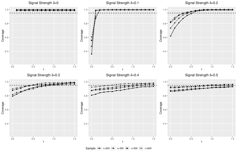
(b) Empirical Coverage of ${\rm CI}_{\Sigma}(\tau)$ defined in (10).

Figure 4: Dense alternative setting: the dependence of Empirical Coverage on $\tau$.

C.2 Additional Simulations for High Correlation Setting

We take the same simulation setting as the high correlation setting in Section 5.3 in the main paper. We vary the signal strength parameter $\delta$ over $\{0,0.1,0.2,0.3,0.4,0.5\}$ and the sample size $n$ over $\{250,350,500,650\}$. We have examined the finite sample performance of the proposed methods over different values of $\tau\in\{0,0.1,0.2,\cdots,1.4,1.5\}.$ The main observations are similar to those reported in Section 5.3 in the main paper.

Regarding the effect $\tau$, the observation is similar to the dense alternative setting reported in Section C.1. $\tau=0.5$ or $\tau=1$ leads to reliable testing and coverage properties and when $\delta$ is above $0.3$, the effect of $\tau$ is marginal. We report the empirical rejection rate for $\phi_{\rm I}(\tau)$ and $\phi_{\Sigma}(\tau)$ in Figure 5 and the coverage properties of the constructed confidence intervals ${\rm CI}_{\rm I}(\tau)$ and ${\rm CI}_{\Sigma}(\tau)$ in Figure 6. The main observations are similar to those in Section C.1. We observe that the test $\phi_{\Sigma}$ is in general more powerful than $\phi_{\rm I}$ and the empirical coverage of both ${\rm CI}_{\rm I}(\tau)$ and ${\rm CI}_{\Sigma}(\tau)$ reaches the desired level even for the high correlation setting.

(a) ERR of $\phi_{\rm I}(\tau)$ defined in (12)

(b) ERR of $\phi_{\Sigma}(\tau)$ defined in (9)

Figure 5: High correlation setting: the dependence of Empirical Rejection Rate (ERR) on $\tau$.

(a) Empirical Coverage of ${\rm CI}_{\rm I}(\tau)$ defined in (13)

(b) Empirical Coverage of ${\rm CI}_{\Sigma}(\tau)$ defined in (10).

Figure 6: High correlation setting: the dependence of Empirical Coverage on $\tau$.

C.3 Dependence on sparsity

We take the same simulation as the dense alternative simulation in Section 5.2, except for generating a sparser regression vector $\beta$: $\beta_{j}=\sqrt{7}\cdot\delta$ for $30\leq j\leq 32$ and $\beta_{j}=0$ otherwise. We consider the same group significance test as in Section 5.2, $H_{0,G}:\beta_{i}=0\;\text{for}\;i\in G,$ with $G=\{30,31,\cdots,200\}.$ The rescaling parameter $\sqrt{7}$ in generating $\beta$ guarantees the same values of $\|\beta_{G}\|_{2}^{2}$ and $\beta_{G}^{\intercal}\Sigma_{G,G}\beta_{G}$ as in the dense alternative setting in Section 5.2. We vary the signal strength parameter $\delta$ over $\{0,0.04,0.06,0.08,0.2,0.4\}$ and the sample size $n$ over $\{250,350,500,650\}$. We have examined the finite sample performance of the proposed method over different values of $\tau\in\{0,0.1,0.2,\cdots,1.4,1.5\}.$

We report the empirical rejection rate for $\phi_{\rm I}(\tau)$ and $\phi_{\Sigma}(\tau)$ in Figure 7 and the coverage properties of the constructed confidence intervals ${\rm CI}_{\rm I}(\tau)$ and ${\rm CI}_{\Sigma}(\tau)$ in Figure 8. By comparing Figure 4 and Figure 8, we observe that for $\delta=0.4$, ${\rm CI}_{\rm I}(\tau)$ achieves the desired coverage level when the sample size $n$ reaches $350.$ This comparison shows that the inference problem is easier for a smaller sparsity level.

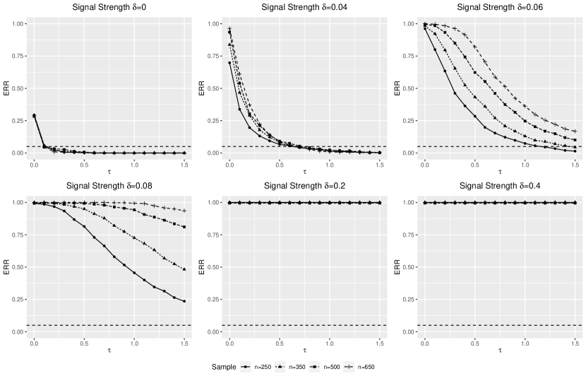
(a) ERR of $\phi_{\rm I}(\tau)$ defined in (12)

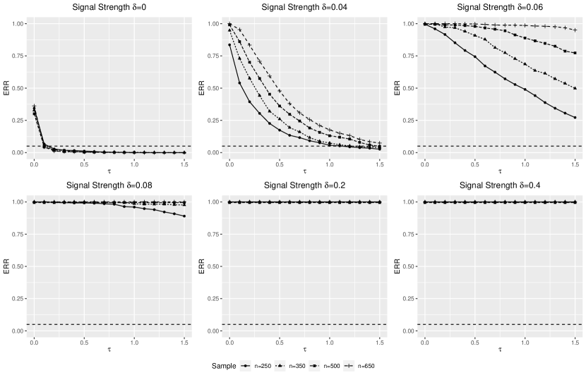
(b) ERR of $\phi_{\Sigma}(\tau)$ defined in (9)

Figure 7: Dense alternative setting with a sparser signal: the dependence of Empirical Rejection Rate (ERR) on $\tau$.

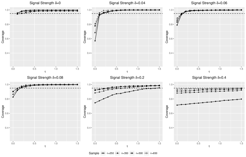
(a) Empirical Coverage of ${\rm CI}_{\rm I}(\tau)$ defined in (13)

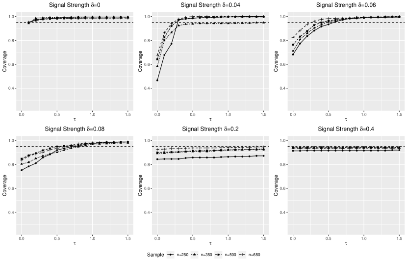
(b) Empirical Coverage of ${\rm CI}_{\Sigma}(\tau)$ defined in (10).

Figure 8: Dense alternative setting with a sparser signal: the dependence of Empirical Coverage on $\tau$.

C.4 Sample splitting

We implement the sample-splitting estimator detailed in (14). Recall that this sample splitting estimator is mainly created to facilitate the proof. We take the same simulation settings as in Section 5.2. We vary the signal strength parameter $\delta$ over $\{0,0.04,0.06,0.08,0.2,0.4\}$ and the sample size $n$ over $\{250,350,500,650,800\}$. We have examined the finite sample performance of the proposed method over different values of $\tau\in\{0,0.1,0.2,\cdots,1.4,1.5\}.$ We report the empirical rejection rate for $\phi_{\rm I}(\tau)$ and $\phi_{\Sigma}(\tau)$ in Figure 9 and the coverage properties of the constructed confidence intervals ${\rm CI}_{\rm I}(\tau)$ and ${\rm CI}_{\Sigma}(\tau)$ in Figure 10. In comparison to the results in Section C.1, we observe that the proposed tests are less powerful than the corresponding tests using full sample and the empirical coverage of the constructed confidence intervals is lower than that using the full data. This loss of efficiency is as expected as only half of the sample are used to construct the initial estimator and the other half are used to correct the bias.

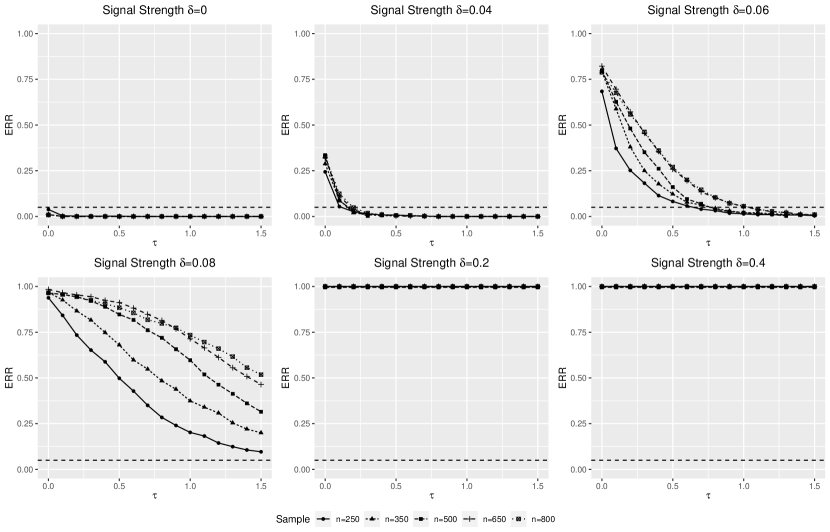
(a) ERR of $\phi_{\rm I}(\tau)$ defined in (12)

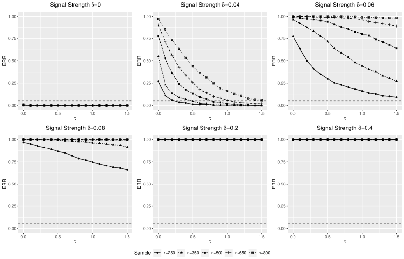
(b) ERR of $\phi_{\Sigma}(\tau)$ defined in (9)

Figure 9: Sample splitting estimators for the dense alternative setting: the dependence of Empirical Rejection Rate (ERR) on $\tau$.

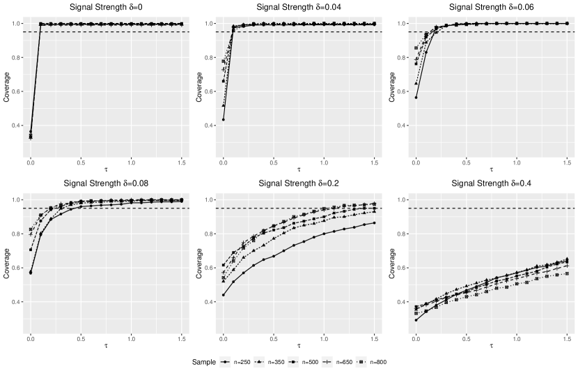
(a) Empirical Coverage of ${\rm CI}_{\rm I}(\tau)$ defined in (13)

(b) Empirical Coverage of ${\rm CI}_{\Sigma}(\tau)$ defined in (10).

Figure 10: Sample splitting estimators for the dense alternative setting: the dependence of Empirical Coverage on $\tau$.

C.5 High-dimensional setting with $p=4,000$

We consider the group significance inference for a higher dimension with $p=4,000$. We vary the sample size across $\{500,1000,2000\}$ to mimic the dimension and the sample size of the colony growth data in Section 5.5. Regarding the generating parameters, we mimic Section 5.2, where the regression vector $\beta\in\mathbb{R}^{4000}$ is generated as $\beta_{j}=\delta$ for $25\leq j\leq 50$ and $\beta_{j}=0$ otherwise and generate the covariance matrix $\Sigma_{ij}=0.6^{|i-j|}$ for $1\leq i,j\leq 4,000$. We consider the group significance test, $H_{0,G}:\beta_{i}=0\;\text{for}\;i\in G,$ with $G=\{30,31,\cdots,200\}$ or $G=\{30,31,\cdots,60\}.$ We vary the signal strength parameter $\delta$ over $\{0,0.08,0.2,0.4\}$.

We report the empirical rejection rate of $\phi_{\Sigma}(\tau)$ defined in (9) in Figure 11. The results are similar to the results for dense alternative presented in Section 5.2 and C.1: for the null setting with $\delta=0$, the testing procedure controls the type I error for $\tau\geq 0.1$; for the alternative settings, the proposed test is powerful when $\delta$ reaches $0.08.$ The observations are uniform for testing both a larger group with $G=\{30,31,\cdots,200\}$ or a smaller group with $G=\{30,31,\cdots,60\}.$

We report the empirical coverage of the confidence interval construction ${\rm CI}_{\rm I}(\tau)$ defined in (10) in Figure 12. We can take $\tau=0.5$ or $1$ and in most settings, the empirical coverages are reliable when $n$ reaches $1,000$, which corresponds to the sample size for the colony growth data in Section 5.5. We note that, for $n=500$, the empirical coverages do not reach $95\%$ though the corresponding tests can still detect the signals when $\delta$ reaches $0.08.$

(a) Test of $\beta_{G}=0$ with $G=\{30,31,\cdots,200\}$

(b) Test of $\beta_{G}=0$ with $G=\{30,31,\cdots,60\}$

Figure 11: High-dimensional setting with $p=4,000$: the dependence of Empirical Rejection Rate (ERR) of $\phi_{\Sigma}(\tau)$ defined in (9) on $\tau$.

(a) Empirical Coverage of ${\rm CI}_{\rm I}(\tau)$ for $\beta_{G}^{\intercal}\Sigma_{G,G}\beta_{G}$ with $G=\{30,31,\cdots,200\}$

(b) Empirical Coverage of ${\rm CI}_{\rm I}(\tau)$ for $\beta_{G}^{\intercal}\Sigma_{G,G}\beta_{G}$ with $G=\{30,31,\cdots,60\}$.

Figure 12: High-dimensional setting with $p=4,000$: the dependence of Empirical Coverage of ${\rm CI}_{\Sigma}(\tau)$ defined in (10) on $\tau$.

C.6 Additional Real Data Analysis for the Yeast Colony Growth Data

Figure 13 describes the results for the colony data set from Section 5.5, but now for all 46 traits.

(a) Traits 1 until 23.

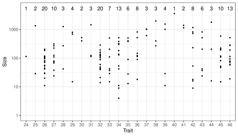
(b) Traits 24 until 46.

Figure 13: Size of significant groups (FWER level $5\%$) by applying the hierarchical procedure to each of the 46 traits of the Yeast Colony Growth data set. The number of significant groups is displayed on the top. The top panel is the same as Figure 1 in the main paper.

C.7 Additional Real Data Analysis for the Riboflavin Data

We apply the hierarchical procedure on a data set about Riboflavin production with Bacillus Subtilis, made publicly available by Bühlmann et al., (2014). It consists of $n=71$ samples of strains of Bacillus Subtilis with response being riboflavin (vitamin $\mbox{B}_{2}$) production rate and covariates measuring the log-expression levels of $p=4088$ genes.

The hierarchical procedure using our group test $\phi_{\Sigma}(\tau=1)$ goes top-down through a hierarchical cluster tree which was estimated using $1-(\text{empirical correlation})^{2}$ as dissimilarity measure and average linkage. The results of the hierarchical procedure are displayed in Table 7. Hierarchical testing finds two single covariates, five small groups, and two large groups. The debiased estimator as implemented in the R package hdi (Dezeure et al.,, 2015) cannot reject any of the single covariates (when testing for all single covariates and adjusting p-values for controlling the FWER). Hence, the maximum test cannot reject the global null hypothesis, implying that no significant group is found using hierarchical testing.

$p$-value	significant cluster
6.113e-09	LICT_at, GLYQ_at, PROA_at, HEME_at, PCP_at, … [5]
1.438e-05	MURE_at, YCGB_at, YQEU_at, SPOVC_at, THDF_at, … [106]
0.0002475	YWAE_at, YQZH_at, YSGA_at, YVDJ_at, YQJU_at, … [2]
$<$ 2.2e-16	LYSC_at, YDBH_at, YDJL_at, YDJK_at, YHXA_at, … [2]
0.0047295	YEBC_at
1.768e-10	CSPD_at, OPUAB_at, OPUAC_at, OPUAA_at, YLNA_at, … [924]
0.0001776	YOAB_at
$<$ 2.2e-16	XLYA_at, YBFG_at, XHLA_at, XHLB_at, XTMA_at, … [9]
1.455e-11	YXLE_at, YXLF_at, YXLC_at, YXLD_at, YXLG_at

Table 7: Results from applying the hierarchical procedure to the Riboflavin data set (FWER level $5\%$). The number in square brackets indicates the number of covariates which are not displayed in the table, i.e. $[2]$ means that two covariates are not displayed for this group.

References

• Arias-Castro et al., (2011) Arias-Castro, E., Candès, E. J., and Plan, Y. (2011). Global testing under sparse alternatives: Anova, multiple comparisons and the higher criticism. The Annals of Statistics, 39(5):2533–2556.
• Belloni et al., (2011) Belloni, A., Chernozhukov, V., and Wang, L. (2011). Square-root lasso: pivotal recovery of sparse signals via conic programming. Biometrika, 98(4):791–806.
• Bickel et al., (2009) Bickel, P. J., Ritov, Y., and Tsybakov, A. B. (2009). Simultaneous analysis of lasso and dantzig selector. The Annals of Statistics, 37(4):1705–1732.
• Bloom et al., (2013) Bloom, J. S., Ehrenreich, I. M., Loo, W. T., Lite, T.-L. V., and Kruglyak, L. (2013). Finding the sources of missing heritability in a yeast cross. Nature, 494(7436):234–237.
• Bühlmann et al., (2014) Bühlmann, P., Kalisch, M., and Meier, L. (2014). High-dimensional statistics with a view towards applications in biology. Annual Review of Statistics and its Applications, 1:255–278.
• Buzdugan et al., (2016) Buzdugan, L., Kalisch, M., Navarro, A., Schunk, D., Fehr, E., and Bühlmann, P. (2016). Assessing statistical significance in multivariable genome wide association analysis. Bioinformatics, 32:1990–2000.
• Cai et al., (2019) Cai, T., Cai, T., and Guo, Z. (2019). Individualized treatment selection: An optimal hypothesis testing approach in high-dimensional models. arXiv preprint arXiv:1904.12891.
• Cai and Guo, (2017) Cai, T. T. and Guo, Z. (2017). Confidence intervals for high-dimensional linear regression: Minimax rates and adaptivity. The Annals of Statistics, 45(2):615–646.
• Cai and Guo, (2020) Cai, T. T. and Guo, Z. (2020). Semi-supervised inference for explained variance in high-dimensional linear regression and its applications. Journal of the Royal Statistical Society: Series B, 82:391–419.
• Chernozhukov et al., (2018) Chernozhukov, V., Chetverikov, D., Demirer, M., Duflo, E., Hansen, C., Newey, W., and Robins, J. (2018). Double/debiased machine learning for treatment and structural parameters. The Econometrics Journal, 21(1):C1–C68.
• Chernozhukov et al., (2017) Chernozhukov, V., Chetverikov, D., and Kato, K. (2017). Central limit theorems and bootstrap in high dimensions. The Annals of Probability, 45(4):2309–2352.
• Dezeure et al., (2015) Dezeure, R., Bühlmann, P., Meier, L., and Meinshausen, N. (2015). High-dimensional inference: Confidence intervals, p-values and R-software hdi. Statistical Science, 30(4):533–558.
• Dezeure et al., (2017) Dezeure, R., Bühlmann, P., and Zhang, C.-H. (2017). High-dimensional simultaneous inference with the bootstrap. Test, 26(4):685–719.
• Friedman et al., (2010) Friedman, J., Hastie, T., and Tibshirani, R. (2010). Regularization paths for generalized linear models via coordinate descent. Journal of Statistical Software.
• Guo et al., (2019) Guo, Z., Wang, W., Cai, T. T., and Li, H. (2019). Optimal estimation of genetic relatedness in high-dimensional linear models. Journal of the American Statistical Association, 114(525):358–369.
• Guo and Zhang, (2019) Guo, Z. and Zhang, C.-H. (2019). Local inference in additive models with decorrelated local linear estimator. arXiv preprint arXiv:1907.12732.
• Hartigan, (1975) Hartigan, J. (1975). Clustering Algorithms. Wiley.
• Ingster et al., (2010) Ingster, Y. I., Tsybakov, A. B., and Verzelen, N. (2010). Detection boundary in sparse regression. Electronic Journal of Statistics, 4:1476–1526.
• Javanmard and Montanari, (2014) Javanmard, A. and Montanari, A. (2014). Confidence intervals and hypothesis testing for high-dimensional regression. Journal of Machine Learning Research, 15(1):2869–2909.
• Klasen et al., (2016) Klasen, J. R., Barbez, E., Meier, L., Meinshausen, N., Bühlmann, P., Koornneef, M., Busch, W., and Schneeberger, K. (2016). A multi-marker association method for genome-wide association studies without the need for population structure correction. Nature Communications, 7:13299.
• (21) Mandozzi, J. and Bühlmann, P. (2016a). Hierarchical testing in the high-dimensional setting with correlated variables. Journal of the American Statistical Association, 111:331–343.
• (22) Mandozzi, J. and Bühlmann, P. (2016b). A sequential rejection testing method for high-dimensional regression with correlated variables. International Journal of Biostatistics, 12:79–95.
• Meinshausen, (2008) Meinshausen, N. (2008). Hierarchical testing of variable importance. Biometrika, 95(2):265–278.
• Meinshausen, (2015) Meinshausen, N. (2015). Group bound: confidence intervals for groups of variables in sparse high dimensional regression without assumptions on the design. Journal of the Royal Statistical Society: Series B (Statistical Methodology), 77(5):923–945.
• Meinshausen et al., (2009) Meinshausen, N., Meier, L., and Bühlmann, P. (2009). P-values for high-dimensional regression. Journal of the American Statistical Association, 104(488):1671–1681.
• Mitra and Zhang, (2016) Mitra, R. and Zhang, C.-H. (2016). The benefit of group sparsity in group inference with de-biased scaled group lasso. Electronic Journal of Statistics, 10(2):1829–1873.
• Raskutti et al., (2010) Raskutti, G., Wainwright, M. J., and Yu, B. (2010). Restricted eigenvalue properties for correlated gaussian designs. Journal of Machine Learning Research, 11:2241–2259.
• Renaux et al., (2020) Renaux, C., Buzdugan, L., Kalisch, M., and Bühlmann, P. (2020). Hierarchical inference for genome-wide association studies: a view on methodology with software. Computational Statistics, 35(1):1–40.
• Shi et al., (2016) Shi, H., Kichaev, G., and Pasaniuc, B. (2016). Contrasting the genetic architecture of 30 complex traits from summary association data. The American Journal of Human Genetics, 99(1):139–153.
• Sun and Zhang, (2012) Sun, T. and Zhang, C.-H. (2012). Scaled sparse linear regression. Biometrika, 101(2):269–284.
• Tian et al., (2014) Tian, L., Alizadeh, A. A., Gentles, A. J., and Tibshirani, R. (2014). A simple method for estimating interactions between a treatment and a large number of covariates. Journal of the American Statistical Association, 109(508):1517–1532.
• Tibshirani, (1996) Tibshirani, R. (1996). Regression shrinkage and selection via the lasso. Journal of the Royal Statistical Society. Series B (Methodological), 58(1):267–288.
• van de Geer et al., (2014) van de Geer, S., Bühlmann, P., Ritov, Y., and Dezeure, R. (2014). On asymptotically optimal confidence regions and tests for high-dimensional models. The Annals of Statistics, 42(3):1166–1202.
• van de Geer and Stucky, (2016) van de Geer, S. and Stucky, B. (2016). $\chi^{2}$-confidence sets in high-dimensional regression. In Statistical analysis for high-dimensional data, pages 279–306. Springer.
• Verzelen and Gassiat, (2018) Verzelen, N. and Gassiat, E. (2018). Adaptive estimation of high-dimensional signal-to-noise ratios. Bernoulli, 24(4B):3683–3710.
• Zhang and Zhang, (2014) Zhang, C.-H. and Zhang, S. S. (2014). Confidence intervals for low dimensional parameters in high dimensional linear models. Journal of the Royal Statistical Society: Series B (Statistical Methodology), 76(1):217–242.
• Zhang and Cheng, (2017) Zhang, X. and Cheng, G. (2017). Simultaneous inference for high-dimensional linear models. Journal of the American Statistical Association, 112(518):757–768.
• Zhou, (2009) Zhou, S. (2009). Restricted eigenvalue conditions on subgaussian random matrices. arXiv preprint arXiv:0912.4045.