Percolation is Odd

Abstract

We prove a remarkable combinatorial symmetry in the number of spanning configurations in site percolation: for a large class of lattices, the number of spanning configurations with an odd or even number of occupied sites differs by $\pm 1$. In particular, this symmetry implies that the total number of spanning configurations is always odd, independent of the size or shape of the lattice. The class of lattices that share this symmetry includes the square lattice and the hypercubic lattice in any dimension, with a wide variety of boundary conditions.

Published in Physical Review Letters 123 230605 (2019)

I Introduction

Percolation theory started in 1941 with the work of Flory on gelation Flory (1941) and its theoretical framework was formulated 1957 by Broadbent and Hammersley Broadbent and Hammersley (1957). Ever since then, it has been a very active field of research. Despite its maturity, most of what we know about percolation is still based on numerical computations, for which clever algorithms like Hoshen and Kopelman (1976) and Newman and Ziff (2000); *newman:ziff:01 had been developed. In contrast, exact mathematical results are rare and mostly limited to two-dimensional systems of infinite size. Examples include the percolation thresholds for some planar lattices found by Sykes and Essam Sykes and Essam (1963) or the celebrated formulas for the critical spanning probabilities derived from conformal invariance by Cardy Cardy (1992) and Watts Watts (1996).

Exact results for finite systems are even rarer, even in two dimensions. A recent example is the discovery of an equation that connects the average number of clusters and the wrapping probabilities for two-dimensional percolation in periodic lattices of any size Mertens and Ziff (2016).

In this contribution, we present a new combinatorial symmetry in the number of spanning configurations in site percolation. Our result holds exactly for finite systems in all dimensions for a broad class of lattices, including the square and hypercubic lattices, and for a wide variety of boundary conditions. In particular, this symmetry implies that the total number of spanning configurations in these systems is odd, independent of the size or shape of the system.

We were motivated by a startling pattern that we found empirically by exhaustive enumerating spanning configurations on small instances of the square lattice. Let $A_{n,m}(k)$ denote the number of vertically spanning configurations with $k$ occupied sites in a lattice with $m$ rows and $n$ columns, i.e., where there is a path of occupied sites connecting the top row to the bottom row. We can define a bivariate generating function

$$R_{n,m}(p,q)=\sum_{k=0}^{nm}A_{n,m}(k)\,p^{k}\,q^{nm-k}\,.$$ (1)

In particular, $R_{n,m}(-1,1)$ is the difference between the number of spanning configurations with an even or odd number of occupied sites,

$$R_{n,m}(-1,1)=\sum_{\text{$k$ even}}A_{n,m}(k)-\sum_{\text{$k$ odd}}A_{n,m}(k)\,.$$ (2)

When we computed this difference explicitly for the square lattice and for small $n$ and $m$, we found the pattern shown in Table 1. It coincides with

$$R_{n,m}(-1,1)=(-1)^{s(n,m)}$$ (3a)

where

$$s(n,m)=\left\lfloor\frac{m}{2}\right\rfloor n+\left\lceil\frac{m}{2}\right\rceil\,.$$ (3b)

	1	2	3	4	5	6	7	8
1	$-1$	$-1$	$-1$	$-1$	$-1$	$-1$	$-1$	$-1$
2	1	$-1$	1	$-1$	1	$-1$	1	$-1$
3	$-1$	1	$-1$	1	$-1$	1	$-1$	1
4	1	1	1	1	1	1	1	1
5	$-1$	$-1$	$-1$	$-1$	$-1$	$-1$	$-1$	$-1$
6	1	$-1$	1	$-1$	1	$-1$	1	$-1$
7	$-1$	1	$-1$	1	$-1$	1	$-1$	1
8	1	1	1	1	1	1	1	1

Table 1: Values of $R_{n,m}(-1,1)$ for the square lattice with $m$ rows and $n$ columns, for either open or cylindrical boundary conditions.

	1	2	3	4	5	6	7	8
1	$-1$	$-1$	$-1$	$-1$	$-1$	$-1$	$-1$	$-1$
2	1	0	$-1$	1	0	$-1$	1	0
3	$-1$	1	$-2$	3	$-5$	8	$-13$	21
4	1	$-1$	$-3$	0	11	9	$-32$	$-57$
5	$-1$	0	$-5$	$-1$1	$-42$	$-121$	$-393$	$-1204$
6	1	1	$-8$	$-9$	121	0	$-1805$	1909
7	$-1$	$-1$	$-13$	32	$-393$	1805	$-13514$	75135
8	1	0	$-21$	57	1204	$-1909$	$-75135$	0

Table 2: Values of $R_{n,m}(-1,1)$ for the triangular lattice.

In other lattices such as the triangular lattice, the pattern is much more complicated, see Table 2. The result for the square lattice is remarkable since the fact that $R_{n,m}(-1,1)=\pm 1$ implies that the number of spanning configurations with even and odd $k$ is almost identical, and in particular that the total number of spanning configurations is always odd; to our knowledge, this was not known before. Last but not least, the pattern of $\pm 1$’s given by $s(n,m)$ cries out for an explanation.

The paper is organized as follows. We start by proving (3a) and (3b). We then generalize this result to site percolation on the hypercube $\mathbb{Z}^{d}$ and, more generally, to cartesian graph products. Then we present the most general form of our result in terms of percolation on graph stacks. Finally we discuss the computation of $R_{n,m}(-1,1)$ for pairs of matching lattices.

II The Square Lattice

We compute $R_{n,m}(-1,1)$ by constructing a partial matching on the set of spanning configurations: that is, for most spanning configurations $\sigma$ we define a unique partner $\sigma^{\prime}$ which is another spanning configuration, such that $\sigma^{\prime\prime}=\sigma$. Moreover, $\sigma$ and $\sigma^{\prime}$ have opposite parity, since they differ at a single site. As a result, the contribution of each matched pair $(\sigma,\sigma^{\prime})$ cancels in the sum (2). The contribution of the remaining spanning configurations is simple enough that it can be written explicitly.

We number the rows $1,\ldots,m$ from top to bottom, and the columns $1,\ldots,n$ left to right. Let $\sigma$ be a spanning configuration, and suppose that row $2$ is not entirely occupied. Then that row has a leftmost empty site $(\ell,2)$ for some $1\leq\ell\leq n$. We define $\sigma^{\prime}$ by flipping the site $(\ell,1)$ in the top row immediately above this empty site, occupying it if it is unoccupied in $\sigma$ and vice versa.

Since $\sigma$ was a spanning configuration, it has a path from the bottom row to the top row. This path arrives on the top row by passing through two adjacent occupied sites, $(x,2)$ and $(x,1)$ for some $x$. But since $(\ell,2)$ is empty, $x\neq\ell$, and this path still exists in $\sigma^{\prime}$. Thus $\sigma^{\prime}$ is also a spanning configuration, and clearly $\sigma^{\prime\prime}=\sigma$ as claimed.

Let us now assume that the second row of $\sigma$ is completely occupied. Then we look for the topmost even-numbered row $r$ that is not completely occupied. We again find its leftmost empty site $(\ell,r)$, and define $\sigma^{\prime}$ by flipping the site $(\ell,r-1)$ in the odd-numbered row above it. As before, $\sigma$ has a path from the bottom to row $r-1$ which passed through occupied sites $(x,r)$ and $(x,r-1)$ where $x\neq\ell$, and this path still exists in $\sigma^{\prime}$. Moreover, once the path arrives on row $r-1$, it can connect immediately to row $r-2$ above it since that row is completely occupied, and from there to the top of the lattice. Thus $\sigma^{\prime}$ is again a spanning configuration, and $\sigma^{\prime\prime}=\sigma$ as before.

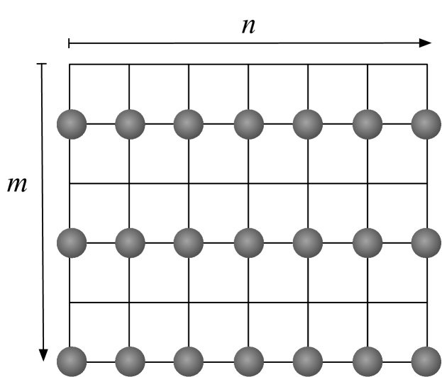
Figure 1: Only configurations in which every even numbered row is fully occupied need to be considered in computing (2).

This defines an opposite-parity partner $\sigma^{\prime}$ for all spanning configurations $\sigma$ except those where all even-numbered rows are fully occupied as shown in Fig. 1. Configurations of this type are spanning configurations if and only if no odd-numbered row is completely empty. If $k_{i}$ denotes the number of occupied sites in row $2i-1$, the total number of occupied sites is

$$\left\lfloor\frac{m}{2}\right\rfloor n+\sum_{i=1}^{\left\lceil\frac{m}{2}\right\rceil}k_{i}\,,$$

since there are $\lfloor m/2\rfloor$ even-numbered rows and $\lceil m/2\rceil$ odd-numbered ones. The number of such configurations is

$${n\choose k_{1}}\,{n\choose k_{2}}\,\cdots\,{n\choose k_{\left\lceil\frac{m}{2}\right\rceil}}\,,$$

so (2) becomes

$$R_{n,m}(-1,1) =(-1)^{\lfloor m/2\rfloor n}\,\prod_{i=1}^{\lceil m/2\rceil}\sum_{k_{i}=1}^{n}{n\choose k_{i}}\,(-1)^{k_{i}}$$

$$=(-1)^{\lfloor m/2\rfloor n}\,\left(\sum_{k=1}^{n}{n\choose k}\,(-1)^{k}\right)^{\lceil m/2\rceil}$$

$$=(-1)^{\lfloor m/2\rfloor n+\lceil m/2\rceil}\,,$$

where we used the fact that $\sum_{k=0}^{n}{n\choose k}(-1)^{k}=(1-1)^{n}=0$. This proves (3a) and (3b).

III Graph Products and Boundary Conditions

The $n\times m$ square lattice with open boundary conditions can be written as the Cartesian graph product $L_{n}\times L_{m}$ Harary (1969) where $L_{n}$ is the path with $n$ vertices. Let us now consider graphs of the form $G\times L_{m}$. Each row or “layer” $1\leq r\leq m$ is a copy of $G$, where each vertex $(v,r)$ is connected to the corresponding vertices $(v,r\pm 1)$ in the rows above and below it. For instance, if we use cylindrical boundary conditions in the horizontal direction, we obtain $C_{n}\times L_{m}$ where $C_{n}$ is the cycle with $n$ vertices.

What properties of $G$, if any, did we use in our proof of (3)? Suppose $r$ is the topmost even-numbered layer which is not fully occupied. Choosing the “leftmost” empty site $(v,r)$ in this layer can be replaced by choosing the first empty site $v$ in an arbitrary fixed ordering of the vertices of $G$. When we defined $\sigma^{\prime}$ by flipping the site $(v,r-1)$ above this empty site, we claimed that this cannot disrupt the way the spanning path in $\sigma$ from the bottom of the lattice first arrives at layer $r-1$, since that path must go through occupied sites $(u,r)$ and $(u,r-1)$ for some $u\neq v$. As long as $G$ is connected, we can then reach any vertex in the fully occupied layer $r-2$, and from there reach the top of the lattice where $r=1$.

Thus for any connected graph $G$, we have

$$R_{G\times L_{m}}(-1,1)=(-1)^{s(n,m)}\,,$$ (4)

where $n$ denotes the number of vertices of $G$ and where we define a spanning configuration as one with a path of occupied sites from the top layer $G\times\{1\}$ to the bottom layer $G\times\{m\}$ of the lattice. This includes the case where $G$ is the $n_{1}\times\cdots\times n_{d-1}$ hypercubic lattice and $n=n_{1}n_{2}\cdots n_{d-1}$, with any boundary conditions (open, cylindrical, toroidal, etc.). Thus (4) holds for the $d$-dimensional hypercubic lattice with any boundary conditions that are open in the vertical direction $n_{d}=m$. It also includes, for instance, the hexagonal crystal lattice in three dimensions where $G$ is a triangular lattice.

IV Graph Stacks

The graph product $G\times L_{m}$ consists of $m$ identical layers, each of which is a copy of $G$. But in our proof of (3) we did not assume that the layers are identical. Hence (4) holds in an even more general setting, where the layers $G_{1},G_{2},\ldots,G_{m}$ are arbitrary connected graphs, each with $n$ vertices labeled $1,\ldots,n$ arbitrarily. The edges $\big{(}(u,r),(v,r)\big{)}$ within each layer $r$ coincide with the edges $(u,v)$ of $G_{r}$, and the edges between layers are $\big{(}(v,r),(v,r\pm 1)\big{)}$ for all $1\leq v\leq n$.

Such graphs have been considered in the study of dynamic networks, e.g. Holme and Saramäki (2012); Ghasemian et al. (2016). Since there is no concept of time here, we prefer to call this construction a graph stack and notate it $[G_{1},G_{2},\ldots,G_{m}]$. We again define a spanning configuration as one with a path from the top layer to the bottom layer. Then

$$R_{[G_{1},\ldots,G_{m}]}(-1,1)=(-1)^{s(n,m)}\,.$$ (5)

This seems to be the most general case for which (3) holds. Physically, it would hold, for instance, if each layer is a connected subgraph of some $(d-1)$-lattice (perhaps with some edges removed by dilution) or if each layer has a different lattice structure entirely.

V Matching Lattices

For lattices outside the class described in the previous section, our method to compute $R(-1,1)$ does not work. Yet for some two-dimensional lattices we can get at least partial results. For that we need the idea of the matching graph. A pair of graphs $(G,\hat{G})$ on the same vertex set is called a matching pair if both $G$ and $\hat{G}$ can be derived from an underlying planar graph $H$ in the following way. Let $F$ be the set of all faces of $H$. Then for some subset $U\subseteq F$, define $G$ (resp. $\hat{G}$) as a copy of $H$ with additional edges such that each face in $U$ (resp. $F\setminus U$) becomes a clique, i.e., a fully connected graph. Note that this definition is symmetric, so that $(G,\hat{G})$ is a matching pair if and only if $(\hat{G},G)$ is.

For example, by taking $H$ to be the square lattice and $U=\emptyset$, we see that if $G$ is the simple square lattice then its matching graph $\hat{G}$ is the square lattice with nearest and next-nearest neighbors (the Moore neighborhood). Similarly, the triangular lattice is self-matching: we can take $G$, $\hat{G}$, and $H$ all to be the triangular lattice, since its faces are already cliques.

The crucial property of a matching pair of lattices is that a configuration with $k$ occupied sites in an $n\times m$ lattice $G$ spans the $m$-direction if and only if the complementary configuration consisting of the $nm-k$ empty sites does not span the $n$-direction in the matching lattice $\hat{G}$ Mertens and Ziff (2016). In other words, in each configuration, either the $k$ occupied sites span in the $m$ direction of $G$, or the $nm-k$ empty sites span the $n$ direction on $\hat{G}$:

$$A_{n,m}(k)+\hat{A}_{m,n}(mn-k)={{nm}\choose k}\,,$$ (6)

where $\hat{A}_{m,n}(k)$ denotes the number of spanning configurations on $\hat{G}$. Multiplying this equation by $p^{k}q^{nm-k}$ and summing over $k$ provides us with

$$R_{n,m}(p,q)+\hat{R}_{m,n}(q,p)=(p+q)^{nm}\,,$$ (7)

where $R$ and $\hat{R}$ are the generating functions (1) for spanning configurations in $G$ and $\hat{G}$ respectively. Along with the general relation

$$R_{n,m}(p,q)=\left(\frac{q}{p}\right)^{nm}R_{n,m}(q^{-1},p^{-1})\,,$$ (8)

which also also holds for $\hat{R}$, we can then write

$$R_{n,m}(p,q)+\left(\frac{q}{p}\right)^{nm}\hat{R}_{m,n}(p^{-1},q^{-1})=(p+q)^{nm}\,,$$ (9)

and in particular

$$R_{n,m}(-1,1)+(-1)^{nm}\hat{R}_{m,n}(-1,1)=0\,.$$ (10)

Now for self-matching lattices like the triangular lattice, we can take off the hat to get

$$R_{n,m}^{\triangle}(-1,1)+(-1)^{nm}R_{m,n}^{\triangle}(-1,1)=0\,.$$ (11)

This tells us that if $m=n$ and $mn$ is even, the balance between even and odd spanning configurations is perfect,

$$R_{n,n}^{\triangle}(-1,1)=0\qquad\text{($n$ even).}$$ (12)

This pattern is visible in Table 2, where the diagonal entries with even $n$ are zero. For other values of $mn$, we only have the symmetry $R_{n,m}^{\triangle}(-1,1)=-(-1)^{nm}R_{m,n}^{\triangle}(-1,1)$. This also shows in Tab. 2, but implies no constraint on the number of configurations.

If, on the other hand, we know $R_{n,m}(-1,1)$ for a lattice $G$, we can use (10) to compute the corresponding function for the matching lattice. Our results on the square lattice imply that for the matching lattice with the Moore neighborhood, we have

$$\hat{R}_{n,m}(-1,1)=-(-1)^{nm+s(m,n)}\,,$$ (13)

which also implies that the total number of spanning configurations is odd for this lattice.

	1	2	3	4	5	6	7	8	9	10
1	1	1	1	1	1	1	1	1	1	1
2	1	0	1	1	0	1	1	0	1	1
3	1	1	0	1	1	0	1	1	0	1
4	1	1	1	0	1	1	0	1	1	0
5	1	0	1	1	0	1	1	0	1	1
6	1	1	0	1	1	0	1	1	0	1
7	1	1	1	0	1	1	0	1	1	0
8	1	0	1	1	0	1	1	0	1	1
9	1	1	0	1	1	0	1	1	0	1
10	1	1	1	0	1	1	0	1	1	0

Table 3: Total number of spanning configurations mod 2 for the triangular lattice with open boundary conditions.

Although there is no simple pattern in $R_{n.m}^{\triangle}(-1,1)$, there appears to be an interesting pattern in the parity of the total number of spanning configurations, i.e., $R_{n.m}^{\triangle}(1,1)$. Table 3 shows this pattern for $n,m\leq 10$. For $n,m>1$ it appears that

$$R_{n,m}^{\triangle}(1,1)\bmod 2=\begin{cases}0&\text{if $n-m=0\bmod 3$,}\\ 1&\text{otherwise.}\end{cases}$$ (14)

Proving this equation would require a different approach than the one used in this paper, but the self-matching property of the trangular lattice gives some information. Since the total number of spanning configurations is given by $R_{n,m}(1,1)$, we can use (10) and the self-matching property to get

$$R_{n,m}^{\triangle}(1,1)+R_{m,n}^{\triangle}(1,1)=2^{nm}\,.$$ (15)

This tells us, that for $n=m$ exactly half of the $2^{n^{2}}$ configurations are spanning, and that the parity matrix $R_{n,m}^{\triangle}(1,1)\bmod 2$ is symmetric. This is not sufficient to prove (14). We leave this as an open question.

VI Conclusions

In the theory of computational complexity Moore and Mertens (2011), counting problems—specifically, counting solutions to a problem where each solution can be verified in polynomial time—constitute the complexity class #P. Computing the coefficients of the generating function $R_{G}(p,q)$ for a general graph $G$ falls into this class. For general graphs, the generating function $R_{G}(p,q)$ is also known as the reliability polynomial, and its computation has been shown to be #P-complete Valiant (1979a), meaning that it is among the hardest counting problems in this class. As a result, we believe that any algorithm needs to perform some kind of explicit enumeration, and therefore requires exponential time. This is true even when $G$ is restricted to planar graphs with bounded degree Provan (1986).

Computing a generating function like $R_{G}(p,q)$ at arbitrary values of $p$ and $q$ is just as hard as computing its coefficients, since we can recover its coefficients by interpolation. However, many generating functions that are #P-complete to compute in general can be efficiently computed at specific points, such as the Tutte polynomial Jaeger et al. (1990). Similarly, computing the parity of a counting problem may or may not be difficult. The permanent of a matrix with $\{0,1\}$ entries is #P-complete Valiant (1979b), but its parity is easy since the permanent and determinant are equivalent modulo $2$. On the other hand, solving general counting problems mod $2$ is probably very difficult, since a polynomial-time algorithm with access to an oracle for such problems can solve any problem in the polynomial hierarchy, including problems well beyond NP-completeness Toda (1991).

In this contribution we have shown that for a large class of lattices we can compute $R_{G}(-1,1)$, i.e., the difference between the number of spanning configurations with an even or odd number of occupied sites. In particular, we have shown that these sets of configurations are almost perfectly balanced. In addition to implying that the parity of the total number of spanning configurations is odd, this almost-perfect balance can be used as a sanity check for enumeration algorithms that compute the numbers $A_{n,m}(k)$ for small values on $n$ and $m$.

We note that since our preprint appeared, alternate proofs were given by Appert-Rolland and Hilhorst Appert-Rolland and Hilhorst (2019) that the number of spanning configurations is odd (though without the symmetry between odd and even $k$) and by Karzes using a transfer matrix approach (unpublished).