Detecting Depinning and Nonequilibrium Transitions with Unsupervised Machine Learning

Abstract

Using numerical simulations of a model disk system, we demonstrate that a machine learning generated order parameter can detect depinning transitions and different dynamic flow phases in systems driven far from equilibrium. We specifically consider monodisperse passive disks with short range interactions undergoing a depinning phase transition when driven over quenched disorder. The machine learning derived order parameter identifies the depinning transition as well as different dynamical regimes, such as the transition from a flowing liquid to a phase separated liquid-solid state that is not readily distinguished with traditional measures such as velocity-force curves or Voronoi tessellation. The order parameter also shows markedly distinct behavior in the limit of high density where jamming effects occur. Our results should be general to the broad class of particle-based systems that exhibit depinning transitions and nonequilibrium phase transitions.

I Introduction

Principal component analysis (PCA) is a linear algebra algorithm that is widely used for identifying patterns in data sets Abdi and Williams (2010). PCA determines the axes along which a data set has the largest variance by expressing the set as a linear sum of basis vectors. The principal components (PC) are the eigenvectors of the data matrix eigenvalue, and the first principal eigenvector has the largest possible eigenvalue. PCA is closely related to single vector decomposition, as detailed in Ref. Shlens (2014), a primer on the mathematics of PCA. Applications of PCA include whitening data and reducing the dimensionality of the system. Often researchers with large data sets use PCA as a tool to reveal a hidden underlying relationship among variables by changing the basis in which the data is expressed and computing the principal components. In reducible data sets, the sum of basis vectors can be truncated while maintaining a reasonable approximation of the original data.

PCA in conjunction with machine learning is used in a broad range of fields where large data sets are common and the underlying relationship between the variables may not be apparent, such as in biology McKinney et al. (2006); Pang et al. (2016) and pattern recognition Bishop (2006). Use of PCA requires the construction of a feature matrix, where a feature is a general name for a measurement of a system. Typically, the feature matrix contains data trials along its rows, which are often called samples in machine learning, and different features along its columns. For example, in facial recognition applications, the pixel values of a digitized photo are used as features, and each photo is considered a sample. The PCA algorithm fits the data and outputs the principal components written as linear combinations of the original features. The algorithm synthesizes information using minimization techniques that maximize the variance along the principal components, which may result from an underlying fundamental physical model.

In condensed matter physics, PCA has successfully been applied to detect phase transitions in the Ising and XY models based on matrices of raw spin configurations Carrasquilla and Melko (2017); Wetzel (2017); Hu et al. (2017); Wang (2016). In a detailed study of various spin models, Hu et al. Hu et al. (2017) confirmed that PCA is well suited for recognizing order and symmetry breaking, and showed that the distribution of principal components can be used to separate strong first order transitions from second order transitions as well as to distinguish phase transitions from pattern changes. Equilibrium phase transitions in a variety of soft matter systems not confined to a lattice can be detected with PCA, such as a density-driven liquid to hexatic phase transition in passive disks Jadrich et al. (2018a, b), where PCA was able to reproduce the qualitative shape of the traditional order parameters. In Ref. Jadrich et al. (2018b) the method was extended to non-equilibrium phase transitions such as random organization Corte et al. (2008). In these studies, the features are constructed intuitively using measures similar to the pair correlation function $g(r)$, which is known to be an excellent indicator of both short and long range order in tightly packed particle systems. Intriguingly, the transformed principal components found by PCA can be related to the packing structures in the disk systems, and by modifying the sampling of the number of probe particles and neighbor particles, it is possible to develop physical insights regarding the shape and magnitude of the order parameter Jadrich et al. (2018b).

Since PCA methods have proven successful at characterizing certain nonequilibrium systems, it is natural to apply these methods in systems that exhibit depinning transitions when individual particles, groups of particles, or elastically coupled elements are driven over quenched disorder Corte et al. (2008); Reichhardt and Reichhardt (2017). Such behavior arises for the depinning of magnetic vortex lines in type-II superconductors Bhattacharya and Higgins (1993); Koshelev and Vinokur (1994); Reichhardt et al. (1997); Olson et al. (1998); Kolton et al. (1999), magnetic domain walls Atkinson et al. (2003), contact lines Paxson and Varanasi (2013), electron crystals Williams et al. (1991); Cha and Fertig (1994); Reichhardt et al. (2001), stripe and bubble phases, Cooper et al. (2003); Reichhardt et al. (2003); Zhao et al. (2013); Wang et al. (2015), sliding quantum crystals Brussarski et al. (2018), skyrmions Schulz et al. (2012); Nagaosa and Tokura (2013); Reichhardt et al. (2015); Jiang et al. (2017); Legrand et al. (2017); Díaz et al. (2017), sliding charge density waves Grüner (1988); Myers and Sethna (1993); Li et al. (1999), colloids Reichhardt and Olson (2002); Pertsinidis and Ling (2008); Tierno (2012); Bohlein et al. (2012); Vanossi et al. (2012); McDermott et al. (2013), jammed systems with quenched disorder Olson Reichhardt et al. (2012); Graves et al. (2016), sliding friction Cule and Hwa (1996); Tekić et al. (2005); Vanossi et al. (2013), geological systems Carlson and Langer (1989), dislocation dynamics Miguel et al. (2002); Zhou et al. (2015), pattern forming systems Sengupta et al. (2010), and active matter Morin et al. (2017); Sándor et al. (2017). In addition to the depinning transition, these systems can exhibit a wealth of distinct dynamical flow phases along with transitions between these phases, such as depinning into a disordered liquid Koshelev and Vinokur (1994); Olson et al. (1998); Kolton et al. (1999); Reichhardt et al. (2001, 2003); Legrand et al. (2017); Reichhardt and Olson (2002); Pertsinidis and Ling (2008); Tierno (2012) followed by a transition into a moving crystal Bhattacharya and Higgins (1993); Koshelev and Vinokur (1994); Reichhardt et al. (1997, 2015); Díaz et al. (2017); Grüner (1988), moving smectic Kolton et al. (1999); Atkinson et al. (2003); Reichhardt et al. (2003); Zhao et al. (2013); Bohlein et al. (2012); Vanossi et al. (2012); Le Doussal and Giamarchi (1998); Balents et al. (1998); Pardo et al. (1998), or other moving pattern Reichhardt et al. (2003); Zhao et al. (2013); Zhou et al. (2015); Sengupta et al. (2010); Sándor et al. (2017) at higher drives. Traditional methods to characterize these systems include the velocity-force curves, differential conductivity, structure factor, and Voronoi tessellations Reichhardt and Reichhardt (2017); however, there are many cases in which the system exhibits dynamics that appear different to the eye but are not distinct according to these standard order parameters. Thus, the nature of the appropriate order parameter is often not clear. There have been some studies using machine learning algorithms to detect depinning transitions on ferroelectric relaxors using the k-means algorithm Jadrich et al. (2018b). It is, however, an open question whether a PCA generated order parameter can characterize transient and steady state nonequilibrium flow phases, as well as non-equilibrium phase transitions, such as those observed in particle based systems.

In this paper, we apply PCA to driven monodisperse disk systems with quenched disorder. Despite the apparent simplicity of this system, it exhibits not only depinning transitions but also a variety of distinct dynamical phases, including laning, clustering, crystalline, and jammed phases Yang et al. (2017). Often the transitions between these phases only produce weak signatures in the standard order parameters. We demonstrate that PCA can automatically detect the different dynamic behaviors as a function of drive. The features we employ are constructed from intuitive measures similar to the pair correlation function $g(r)$ used in Jadrich et al. Jadrich et al. (2018a, b) We show that the machine learning derived order parameter is superior to the standard order parameters, indicating that combining the pairwise distance information into principal components using PCA can successfully synthesize the fundamental information of the emergent behavior. This method could be applied to a wide variety of other particle-based systems that exhibit depinning.

The paper is organized as follows. In Section II we outline the principal component analysis technique for the depinning system. The simulation details of the disk system, along with the standard measures such as the velocity-force curve and Voronoi tessellation, are described in Section III. We show in Section IV that the principal component analysis of the disk system at different densities can identify distinct changes which correlate with changes in the dynamics and structure of the system, and in Section V we summarize our results.

II Principal Component Analysis of Disk Systems

PCA is designed to discover and maximize correlations in data sets contained in matrices  Hu et al. (2017). The features range from pixel values of the digitized photo in facial recognition applications to the matrix of spin values in spin-based systems. In off-lattice systems, the raw position data does not naturally lend itself to description by an $m$ by $n$ matrix. Thus to apply PCA to disks, it is useful to apply traditional measures of structural information. Here we use a “particle centered” measure in PCA to perform dimensionality reduction on the geometrical environment of the particles themselves, rather than attempting to classify the manner in which particles fit into the container. We consider a 2D system of disks of radius $r$ interacting with a random array of pinning sites, as described in Yang et al. (2017); additional simulation details appear in Section III.

We characterize the structural information of the disks using the relative positional data, $r_{ij}=|{\bf r}_{ij}|$, where ${\bf r}_{ij}={\bf r}_{i}-{\bf r}_{j}$ is the center-to-center distance between disks $i$ and $j$. For a certain subset of probe particles $m=N_{\rm probe}=1000$, we measure the distance from the probe particle to $n$ of its neighbor particles. We sort the resulting distances and place the values into a feature vector for each probe particle $i$,

$$\vec{f}_{i}=[r_{i0},r_{i1},r_{i2},...,r_{ij},...,r_{in}].$$ (1)

such that $r_{i0}<r_{i1}<...<r_{in}$. In a procedure typical for PCA, we center the feature vectors by computing the average of each neighbor distance,

$$\langle r_{j}\rangle_{D}=\frac{1}{N_{\rm probe}}\Sigma_{i=0}^{N_{\rm probe}}{r_{ij}},$$ (2)

in order to create a vector containing a series of averages:

$$\vec{\langle r\rangle}_{D}=[\langle r_{0}\rangle_{D},\langle r_{1}\rangle_{D},...,\langle r_{j}\rangle_{D},...,\langle r_{n}\rangle_{D}].$$ (3)

We subtract $\vec{\langle r\rangle}_{D}$ from each feature vector $\vec{f}_{i}$.

We assemble the centered feature vectors into a feature matrix:

$$\vec{F}=[\vec{f}_{0},\vec{f}_{1},\vec{f}_{2},...,\vec{f}_{m}]^{T}.$$ (4)

To remove the correlations introduced in the sorting process, we perform the essential step of whitening the data, as in Ref Jadrich et al. (2018a, b). The whitening transformation is performed by applying the PCA algorithm to a feature matrix of an ideal gas composed of non-interacting disks at density $\phi$ using the same number of probe $N_{\rm probe}$ and neighbor $n$ disks as in our actual system. The PCA analysis of the ideal gas system generates a transformation matrix, $\vec{W}_{0}(\phi)$, that transforms the ideal gas system with density $\phi$ into a Gaussian distribution with mean zero and variance one. We can then use $\vec{W}_{0}$ to transform feature matrices from non-ideal gas systems with density $\phi$ into a coordinate space in which naive sorting correlations have been removed, preserving only the features that contain correlations due to the particle interactions and external forces. It is necessary to compute a separate $\vec{W}_{0}$ for each density $\phi$.

To implement PCA, we use the incremental PCA library available through Scikit-Learn Pedregosa et al. (2011) in order to process many feature vectors without holding the entire feature matrix in memory. After analyzing the whole data set, the PCA algorithm returns a transformation matrix, $\vec{W}(\phi)$, that can be applied to new data. Here, we generate $\vec{W}$ at fixed density $\phi$ values for all values of $F_{D}$. Thus the algorithm simultaneously “sees” systems above and below the depinning transition in the variety of different phases that are described in Ref. Yang et al. (2017).

In order to apply the PCA algorithm, we run the disk simulation until the system reaches a steady state. Then we sample snapshots of the system, using ten frames spaced by $\Delta t=1\times 10^{5}$ simulation time steps. In each frame we randomly select $m=1000$ probe particles, and for each particle we calculate the distance to its $n$ nearest neighbors. Here we take $n=N_{d}(\phi)-1$, where $N_{d}(\phi)$ is the total number of disks in the sample at density $\phi$, meaning that we calculate the distance from the probe particle to all other particles in the system. For each simulation frame we generate the centered feature vector $\vec{f}_{i}$. This must be prewhitened to obtain $\vec{f}_{i}^{w}=\vec{W}_{0}(\phi)\vec{f}_{i}$. To generate a PCA transformation matrix $\vec{W}(\phi)$ valid for disk density $\phi$, we analyze all feature data from all frames for the given disk density $\phi$ by feeding ten $m\times n$ matrices of prewhitened feature vectors into the incremental PCA algorithm in sequence. The algorithm returns the transformed data $\vec{f}^{\prime}$, eigenvalues $\lambda_{N}$, and the transformation matrix $\vec{W}$. This matrix may be used to transform new prewhitened feature vectors from subsequent snapshots of data obtained at the same value of $\phi$, or it can be applied to the already processed feature vectors in order to generate a visualization of the vectors in the new basis space.

Jadrich et al. Jadrich et al. (2018a, b) showed that the principal components contain structural information of the system, and thus can be used as an order parameter (OP) of the system. To construct such an order parameter, we transform a prewhitened feature vector $\vec{f_{i}}^{w}$ obtained at fixed $F_{D}$ and $\phi$ with the trained PCA model to obtain

$$\vec{p}_{i}=\vec{W}\vec{f}^{w}_{i}.$$ (5)

The order parameter $P_{1}$ is defined to be the extent to which the first principal component captures the information content in the system,

$$P_{1}=\langle|p_{1}|\rangle,$$ (6)

where $p_{1}$ is the first element in $\vec{p}$. We analyze the eigenvalue spectrum using a scree plot to determine how well the matrix can be expressed in the new PC basis. We also plot the magnitude of the first principal component, the total transformation matrix $\vec{Q}=\vec{W}\vec{W}_{0}$ that is remarkably similar to $g(r)$, and the ML derived order parameter $P_{1}=\langle|p_{1}|\rangle$.

III Simulation and System

We analyze the data from our previous publication Yang et al. (2017), in which we performed 2D molecular dynamics simulations of passive disk systems. The system contains $N_{d}$ disks of radius $R_{d}$ within a simulation box of $S_{x}=S_{y}=60.0$, in dimensionless simulation length units, with periodic boundary conditions. The area density is given by $\phi=N_{d}\pi R_{d}^{2}/(S_{x}S_{y})$. In the absence of quenched disorder, the disks form a polycrystalline state near $\phi\approx 0.85$ and a triangular solid at $\phi\approx 0.9$.

The disk dynamics are governed by the following overdamped equation of motion:

$$\eta\frac{d{\bf r}_{i}}{dt}={\bf F}_{dd}+{\bf F}_{p}+{\bf F}_{D}.$$ (7)

Here $\eta$ is the damping constant and ${\bf r}_{i}$ is the location of disk $i$. The disk-disk interaction force is ${\bf F}_{dd}=\sum_{i\neq j}k(2R_{d}-|{\bf r}_{ij}|)\Theta(2R_{d}-|{\bf r}_{ij}|){\hat{\bf r}_{ij}}$, where ${\bf r}_{ij}={\bf r}_{i}-{\bf r}_{j}$, $\hat{\bf r}_{ij}={\bf r}_{ij}/|{\bf r}_{ij}|$, the disk radius $R_{d}=0.5$, and the spring constant $k=50$. Distances are measured in simulation units $l_{0}$ and forces are measured in simulation units $f_{0}$ so that $k$ is in units of $f_{0}/l_{0}$ and the unit of simulation time is $\tau=\eta l_{0}/f_{0}$.

We introduce quenched disorder by placing pinning sites throughout the sample. The pinning force ${\bf F}_{p}$ is modeled as arising from $N_{p}$ randomly placed parabolic attractive wells with a pinning radius of $r_{p}=0.5$, such that only a single disk can be trapped in a given pinning site at any given time. We fix the pinning density to $\phi_{p}=N_{p}/(S_{x}S_{y})=0.314$. The driving force ${\bf F}_{D}=F_{D}{\bf\hat{x}}$ is applied uniformly to all particles and is incremented in steps of $\Delta F_{D}=0.05$ after every $\Delta t=1\times 10^{6}$ simulation time steps. At each drive increment, we measure the average disk velocity $\langle V_{x}\rangle=N_{d}^{-1}\sum^{N_{d}}_{i=1}{\bf v}_{i}\cdot{\hat{\bf x}}$, where ${\bf v}_{i}$ is the instantaneous velocity of disk $i$.

A useful measure for characterizing interacting particles driven over disorder is the fraction $P_{6}$ of sixfold-coordinated particles. Here $P_{6}=N_{d}^{-1}\sum_{i}^{N_{d}}\delta(z_{i}-6)$, where $z_{i}$ is the coordination number of disk $i$ obtained from a Voronoi tessellation. Previously Yang et al. (2017), we correlated local maxima in $P_{6}$ with changes in the dynamic phases, and demonstrated that $P_{6}$ did not have a feature at all of the dynamical phase transitions. This behavior for the disks with short-range interactions differs from what is observed for particles that have longer range interactions, where the dynamic phase changes are more readily detected using information from the Voronoi tessellation.

Figure 1: (a) The average disk velocity $\langle V_{x}\rangle$ vs driving force $F_{D}/F_{p}$ in samples with total disk density $\phi$ of $\phi=0.85$ (down triangles), $0.71$ (pentagons), $0.61$ (right triangles), $0.55$ (stars), $0.43$ (squares), $0.30$ (up triangles), and $0.25$ (circles). (b) The corresponding $P_{6}$ vs $F_{D}/F_{p}$.

IV Results

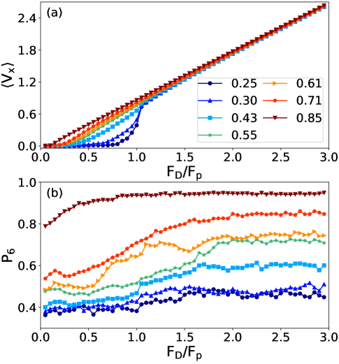
In Fig. 1 we plot the traditional dynamical measurements as a function of $F_{D}/F_{p}$ for a sample with fixed pinning density at different disk densities $\phi$ ranging from $\phi=0.25$ to $\phi=0.85.$ The velocity-force curves $\langle V_{x}\rangle$ versus $F_{D}/F_{p}$ in Fig. 1(a) have the same features that are generically found in systems that undergo depinning. At low drive, there is a pinned regime with $\langle V_{x}\rangle=0.$ This is followed at higher drive by a nonlinear regime above depinning, and at the highest drives, there is a regime in which the velocity increases linearly with increasing $F_{D}$. As the disk density increases, the depinning transition shifts to lower $F_{D}$ and the region of nonlinear velocity response becomes narrower. In Fig. 1(b), the fraction $P_{6}$ of six-fold coordinated disks versus $F_{D}/F_{p}$ is nearly flat for $\phi=0.25$ and $0.3$, while for higher $\phi$ there is some tendency for $P_{6}$ to increase with increasing $F_{D}$. Overall, the results in Fig. 1 indicate that it is difficult to identify distinct dynamic phases using these measures, and that it is even difficult to precisely pinpoint the depinning transition.

Figure 2: Images obtained at a disk density of $\phi=0.30$ for the system in Fig. 1 at $F_{D}=0.25$ (pinned), (b) $F_{D}=0.95$ (phase separated), (c) $F_{D}=1.5$ (smectic flow), and (d) $F_{D}=2.5$ (smectic flow).

IV.1 Low Disk Density

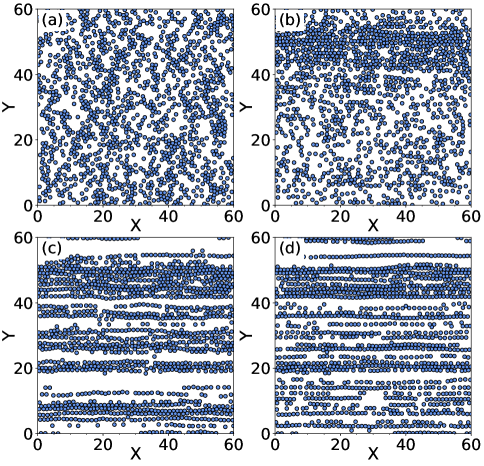
We first focus on the low density limit with $\phi=0.25$ and $\phi=0.3$, where $P_{6}$ is almost featureless. In Fig. 2 we illustrate the disk configurations in a sample with $\phi=0.3$ at different values of $F_{D}/F_{p}$. In the pinned phase at $F_{D}/F_{p}=0.25$, Fig. 2(a) shows that small disordered clusters appear since some of the particles have formed clogged clusters instead of being directly trapped by the pinning sites. Above depinning at $F_{D}/F_{p}=0.95$ in Fig. 2(b), there is a combination of smaller pinned clusters with a phase separated region of higher density in which the disks move in a band. In Fig. 2(c) at $F_{D}/F_{p}=1.5$, all the disks are moving in one-dimensional (1D) chains, while in Fig. 2(d) at $F_{D}=2.5$, the moving chains have become somewhat more rarefied. These results indicate that different dynamical regimes are present which are generally not detectable with the standard measures. We note that other measures such as the structure factor $S(k)$ and diffusion similarly show only weak or no changes at the transitions among these dynamical regimes.

Figure 3: The machine learning derived order parameter $P_{1}$ vs $F_{D}/F_{p}$ for the system in Fig. 1 at disk density $\phi=0.30$. Three phases are clearly apparent: the pinned state at $0<F_{D}/F_{p}<0.65$, the phase separated state at $0.65\leq F_{D}/F_{p}<1.3$, and the smectic or laned state at $F_{D}\geq 1.3$.

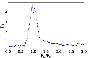
In Fig. 3 we plot the machine learning derived order parameter $P_{1}$ versus $F_{D}/F_{p}$ for the system in Fig. 1. We find $P_{1}\approx 0.5$ for $0<F_{D}/F_{p}<0.65$, which is the pinned state illustrated in Fig. 2(a). This is followed by an increase in $P_{1}$ at $F_{D}/F_{p}=0.65$, corresponding to the depinning transition. $P_{1}$ remains elevated over the range $0.65\leq F_{D}/F_{p}<1.05$ in the phase separated state shown in Fig. 2(b). For $1.05\leq F_{D}/F_{p}<1.25$, $P_{1}$ decreases when the system crosses over into the smectic or laned state. There is a gradual decrease in $P_{1}$ from $P_{1}\approx 1.2$ to $P_{1}\approx 1.0$ over the range $1.25\leq F_{D}/F_{p}\leq 3.0$ as the smectic lanes become increasingly well defined, as shown in Fig. 2(c,d) at $F_{D}/F_{p}=1.5$ and $F_{D}/F_{D}=2.5$. The results in Fig. 3 indicate that $P_{1}$ clearly detects and distinguishes the three phases, pinned, phase separated, and smectic, along with the transitions between these states. For $\phi=0.25$ (not shown), we find similar phases and a similar response of $P_{1}$.

Figure 4: The scaled eigenvalues (relative scores) $\lambda_{N}$ of the PCA algorithm vs the relative ranking $N$ for disk densities of $\phi=0.85$ (down triangles), $0.71$ (pentagons), $0.61$ (right triangles), $0.55$ (stars), $0.43$ (squares), $0.30$ (up triangles), and $0.25$ (circles). $N=1$ corresponds to the first principal component.

IV.2 Eigenvalue Distribution

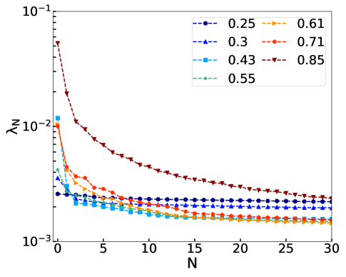
In Fig. 4 we show a scree plot of the eigenvalues $\lambda_{N}$ for the samples in Fig. 1 with disk densities of $\phi=0.25$ to $\phi=0.85$. Here the eigenvalues are sorted from largest ($N=1$) to smallest and plotted versus eigenvalue ranking $N$. The scree plot gives an indication of how successfully the PCA has reduced the dimensionality of the information present in the system. When the eigenvalue spectrum is dominated by one or a few large values of low rank, followed by many small values, it indicates that the first few eigenvectors can be used to describe the primary characteristics of the system, since a linear combination of the first few principal components captures most of the information. At $\phi=0.25$ and $\phi=0.3$, the first eigenvalue $\lambda_{1}$ is somewhat larger in size and the remainder of the eigenvalues are nearly flat. At intermediate disk densities of $\phi=0.43$ to $\phi=0.73$, $\lambda_{1}$ is substantially larger than the remaining eigenvalues, indicating that the PCA analysis has captured the features of the system well. We find a significant jump up in all the eigenvalues at the high density of $\phi=0.85$, which corresponds to the onset of jamming behavior.

IV.3 Intermediate Disk Densities

Figure 5: $P_{1}$ vs $F_{D}/F_{p}$ for the system in Fig. 1 at intermediate disk densities. (a) At $\phi=0.43$, there are multiple peaks. (b) At $\phi=0.61$, the peak structure is more compressed.

Figure 6: Images obtained at a disk density of $\phi=0.43$ for the system in Fig. 5(a) at (a) $F_{D}/F_{p}=0.05$ (disordered pinned state), (b) $F_{D}/F_{p}=0.55$ (clustering clogged state), (c) $F_{D}/F_{p}=0.75$ (moving liquid), (d) $F_{D}/F_{p}=0.95$ (phase separated state with amorphous order), (e) $F_{D}/F_{p}=1.5$ (phase separated state with crystalline order), and (f) $F_{D}/F_{p}=2.5$ (moving smectic).

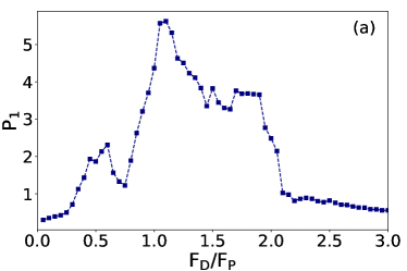
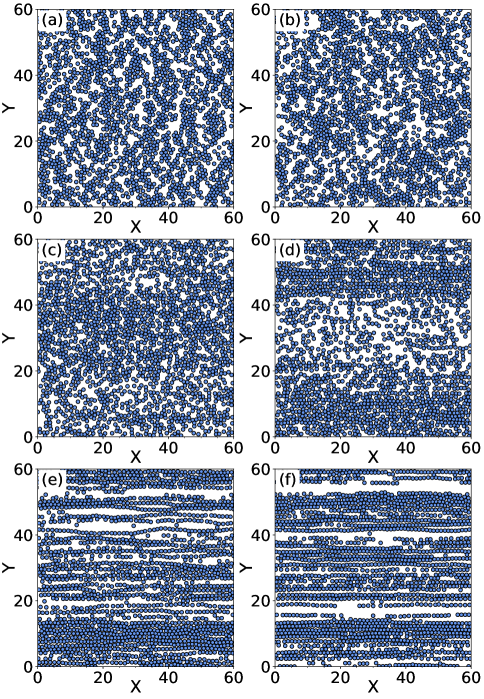
We next consider the intermediate disk density regime. In Fig. 5(a) and (b) we plot $P_{1}$ versus $F_{D}/F_{p}$ for the samples from Fig. 1 with $\phi=0.43$ and $\phi=0.61$, respectively. At both densities, in Fig. 1 $\langle V_{x}\rangle$ versus $F_{D}/F_{p}$ is fairly smooth and $P_{6}$ has a gradual increase, but it is difficult to distinguish different phases from these measures. In contrast, $P_{1}$ in Fig. 5(a) $P_{1}$ has two clear peaks at $F_{D}/F_{p}=0.55$ and $F_{D}/F_{p}=1.0$, a plateau region over the range $1.5<F_{D}<2.0$, and drops to a low value for $F_{D}>2.0$. In Fig. 6(a) we illustrate the disk configuration at $F_{D}/F_{p}=0.05$ within the pinned phase, where $P_{1}$ in Fig. 5(a) is small. Here the disks form small clusters in the pinned state. At $F_{D}/F_{p}=0.55$ in Fig. 6(b), just below the depinning transition, the disks form a locally clustered or clogged state, and at depinning these clusters partially break apart, producing the dip in $P_{1}$ found in Fig. 5(a). A local minimum in $P_{1}$ appears near $F_{D}/F_{p}=0.75$, where the structure is a moving liquid as shown in Fig. 6(c). The amorphous phase separated state at $F_{D}/F_{p}=0.95$ is illustrated in Fig. 6(d). At $F_{D}/F_{p}=1.5$, the system is still phase separated but the amount of crystalline ordering has increased. In Fig. 6(f) the configuration at $F_{D}/F_{p}=2.5$ indicates that the disks have formed a moving smectic state. In general, $P_{1}$ shows a pronounced drop at the transition into the moving smectic states, while the corresponding $P_{6}$ curve for $\phi=0.43$ in Fig. 1 exhibits no feature near $F_{D}/F_{p}=2.5$. This indicates that $P_{1}$ is much more sensitive to the changes in the disk configurations than $P_{6}$ or $\langle V_{x}\rangle$.

Figure 7: Images obtained at a disk density of $\phi=0.61$ for the system in Fig. 5(b) at (a) $F_{D}/F_{p}=0.25$ (pinned clogged state), (b) $F_{D}/F_{p}=0.95$, (phase separated with crystalline order), (c) $F_{D}/F_{p}=1.5$ (moving state), and (d) $F_{D}/F_{p}=2.5$ (moving state).

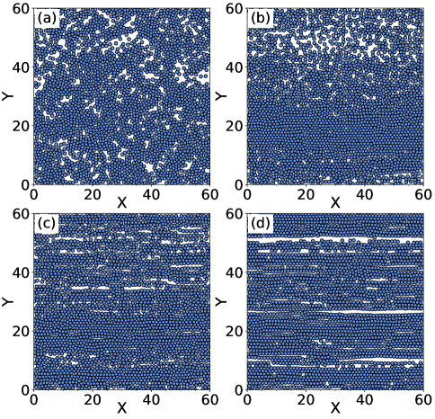
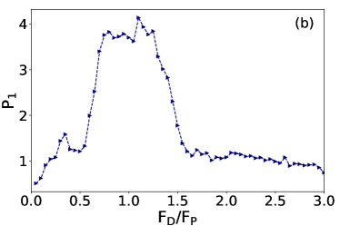
For $\phi=0.61$, Fig. 5(b) shows that $P_{1}$ versus $F_{D}/F_{p}$ has a similar trend as that found for $\phi=0.43$. There are some differences, however; the plateau region in $P_{1}$ is smaller for $\phi=0.61$ and the drop in $P_{1}$ has shifted to a lower value of $F_{D}/F_{p}=1.5$. In Fig. 7(a) we illustrate the disk configuration for the $\phi=0.61$ system at $F_{D}/F_{p}=0.25$, where a pinned clogged state appears. This is the same value of $F_{D}/F_{p}$ at which there is a local peak in $P_{1}$. Figure 7(b) shows the disk configuration at $F_{D}/F_{p}=0.95$, where the system forms a phase separated state with local crystalline ordering. Here $P_{1}=3.85$, which is close to the same value found for $P_{1}$ in the $\phi=0.43$ sample in the phase separated moving crystal phase illustrated in Fig. 6(e) at $F_{D}/F_{p}=1.5$. Thus, at $\phi=0.61$, the moving phase separated amorphous state found at lower $\phi$ is missing. In Fig. 7(c) we show the disk configuration at $F_{D}=1.5$, where the local phase separation is reduced and the system begins to form a moving state. This moving state becomes more pronounced in Fig. 7(d) at $F_{D}=2.5$.

IV.4 High Disk Densities

Figure 8: $P_{1}$ vs $F_{D}/F_{p}$ for the system in Fig. 1 at $\phi=0.85$, where the disks exhibit jamming behavior and elastic depinning.

Figure 9: Images obtained at a disk density of $\phi=0.85$ for the system in Fig. 8, where the system forms a jammed solid with increasing triangular ordering at higher drives. (a) $F_{D}/F_{p}=0.25$. (b) $F_{D}/F_{p}=2.5$.

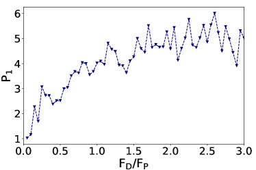
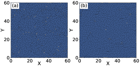
For the lower and intermediate disk densities, there are clear changes in the particle configurations as a function of drive. At high densities of $\phi\geq 0.85$, however, the system becomes a uniform jammed solid and the depinning transition changes in character from plastic, where there can be a coexistence of pinned and moving particles, to elastic, where all the particles keep the same neighbors as they move. There is a distinct change in the eigenvalue distribution in Fig. 4 for $\phi=0.85$, with significant weight appearing at higher values of $N$, indicating a change in the ability of the PC to capture the information in the system. In Fig. 8 we plot $P_{1}$ versus $F_{D}/F_{P}$ for $\phi=0.85$. Instead of peaks, we find a monotonic increase in $P_{1}$ with increasing $F_{D}/F_{P}$. In Fig. 9(a) we illustrate the disk configuration at $F_{D}/F_{P}=0.25$, where the system forms a mostly triangular solid with a small number of vacancies. For $F_{D}/F_{p}=2.5$, shown in Fig. 9(b), the structure is similar but the amount of triangular order is larger. Here the lack of jumps in $P_{1}$ is consistent with the fact that the depinning is elastic and the sample shows no large scale changes in the particle configurations.

Figure 10: First vector $[q_{1}]$ from the total transformation matrix $\vec{Q}$ versus $k$, which is related to a neighbor distance, for the system in Fig. 1 at disk densities $\phi=$ (a) 0.25, (b) 0.43, (c) 0.61, and (d) 0.85.

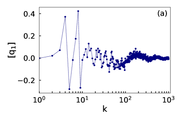
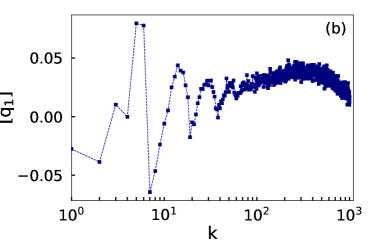
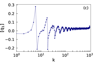
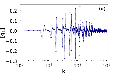
The total transformation matrix $\vec{Q}=\vec{W}\vec{W}_{0}$ provides a physical snapshot of the system not unlike that given by $g(r)$ Jadrich et al. (2018a, b). When applied to a raw feature vector $\vec{f}_{i}$, $\vec{Q}$ first prewhitens the vector through the $\vec{W}_{0}$ matrix, and then transforms the vector into the PC basis through the $\vec{W}$ matrix. The first row of $Q$, termed $[q_{1}]$, is a convolution of the prewhitening transformation and the basis transformation for the first principal component, such that the expression $p_{1}=[q_{1}]\vec{f}_{i}$ gives the mapping of the raw feature vector onto the first principal component. The $k$th component of $[q_{1}]$ provides the mapping of the $k$th component of $\vec{f}_{i}$, and since the elements of $\vec{f}_{i}$ are ordered according to neighbor distance, with the smallest values of $k$ corresponding to the smallest neighbor distances, it is possible to interpret $k$ as a neighbor distance. The prewhitening portion of $[q_{1}]$, plotted as a function of $k$, contains information similar to that found in $g(r)$ of an ideal gas at density $\phi$. The transforming portion of $[q_{1}]$ indicates which neighbor distances are most strongly weighted in the first principal component basis. In Fig. 10 we plot $[q_{1}]$ versus $k$ from a PCA analysis of the monodisperse passive disks at disk densities of $\phi=0.25$, 0.43, 0.61, and 0.85. The prewhitening component produces regular oscillations in $[q_{1}]$ at spacings corresponding to the average distance between successive rings of particles surrounding the probe particle. In an ideal gas, these oscillations would diminish with increasing $k$. The uneven weighting of the oscillations is an indication of which distance scales are important at each density in the first principal component. In Fig. 10(a-c), samples with low and intermediate densities of $\phi=0.25,$ $\phi=0.43,$ and $\phi=0.61$ have large peaks of $[q_{1}]$ at smaller $k$, indicating that the structural ordering is relatively short ranged. In contrast, the high density $\phi=0.85$ sample in Fig. 10(d) has strong weightings at much larger $k$, indicating the long range nature of the emerging crystalline ordering in the jammed state.

V Discussion

We have demonstrated that unsupervised machine learning can detect depinning and the transitions between different dynamical phases in driven systems with quenched disorder. A similar approach could be adapted for systems with longer range particle-particle interactions, such as superconducting vortices Koshelev and Vinokur (1994); Olson et al. (1998); Kolton et al. (1999), charged colloids, and Wigner crystals Cha and Fertig (1994); Reichhardt et al. (2001), which can exhibit a pinned phase, plastic depinning, disordered liquid flow, and a moving crystal or smectic flow phase. In these systems it is often possible to use $P_{6}$ to detect the transitions; however, in some situations, additional transitions could be present that produce no signal in $P_{6}$ but that could be detected using PCA. For example, at a transition from a liquid to a strongly nematic or smectic state, the density of defects in the lattice undergoes little change and therefore the value of $P_{6}$ is constant across the transition, but the PCA could detect the structural change occurring in the system. Additionally, the plastic flow state may be composed of distinct plastic flow phases that have not yet been characterized but that may be detectable using the PCA approach. Depinning of particles on periodic substrates would also be interesting to study since in this system, different types of soliton or incommensurate flow patterns arise. These flow states can often be observed through features in the velocity-force curves, but produce little change in the structure of the particles Reichhardt et al. (1997); Bohlein et al. (2012); Vanossi et al. (2012); McDermott et al. (2013). Here, PCA could be applied to more readily distinguish between the different types of commensurate and incommensurate flows.

PCA could also be applied to the class of systems that exhibit elastic depinning, in which the particles maintain the same neighbors as they begin to flow Reichhardt and Reichhardt (2017). Our disk system at a density of $\phi=0.85$ generally behaves elastically, keeping the same structures at depinning as in the moving phase, and we find that the PCA analysis gives distinctive results for this elastic state compared to the plastic flow phases that appear at lower densities. Elastic depinning can occur for superconducting vortices or skyrmions interacting with weak pinning, or in the depinning of domain walls and elastic lines.

Another future direction is to apply PCA to other measures beyond the particle configurations, such as velocity fluctuations, the velocity-force curves, defect distributions, or local stress. Our results suggest that unsupervised machine learning can be a valuable method for identifying different nonequilibrium phases and the transitions between them. Since the data we employed in our analysis included only the particle locations and not the pinning site locations, a similar approach could be used for any type of particle-based system.

VI Summary

In summary, we have shown that PCA can be used to identify the depinning transition and different nonequilibrium flow phases in a driven system of disks with short-range interactions moving over quenched disorder in the form of randomly placed pinning sites. In this system, traditional methods used to characterize depinning, such as the velocity-force curve and the Voronoi tessellation, show only weak signatures of the different dynamic states. In contrast, the PCA produces pronounced signals at the transitions between the pinned state, the moving phase separated state, and the moving smectic state. Using PCA, we also find evidence for more subtle phase transitions such as a clustered pinned phase as well as a transition between an amorphous and a crystalline phase separated state. The PCA can detect the onset of the jammed state and exhibits different signatures for plastic versus elastic depinning. The PCA method can be used to search for additional features in previously studied depinning systems such as superconducting vortices, Wigner crystals, skyrmions, and charge density wave systems, as well as to identify novel nonequilibrium phases in particle-based systems.