Learning Koopman Eigenfunctions and Invariant Subspaces from Data: Symmetric Subspace Decomposition

Abstract

This paper develops data-driven methods to identify eigenfunctions of the Koopman operator associated to a dynamical system and subspaces that are invariant under the operator. We build on Extended Dynamic Mode Decomposition (EDMD), a data-driven method that finds a finite-dimensional approximation of the Koopman operator on the span of a predefined dictionary of functions. We propose a necessary and sufficient condition to identify Koopman eigenfunctions based on the application of EDMD forward and backward in time. Moreover, we propose the Symmetric Subspace Decomposition (SSD) algorithm, an iterative method which provably identifies the maximal Koopman-invariant subspace and the Koopman eigenfunctions in the span of the dictionary. We also introduce the Streaming Symmetric Subspace Decomposition (SSSD) algorithm, an online extension of SSD that only requires a small, fixed memory and incorporates new data as is received. Finally, we propose an extension of SSD that approximates Koopman eigenfunctions and invariant subspaces when the dictionary does not contain sufficient informative eigenfunctions.

I Introduction

Driven by advances in processing, data storage, cloud services, and algorithms, the world has witnessed in recent years a revolution in data-driven learning, analysis, and control of dynamical phenomena. State-space, probabilistic, and neural network models are among the most popular methods to model dynamical systems. With sufficient a priori information about the dynamics, state-space methods can provide closed-form analytic models that describe accurately the dynamical behavior. Such models, however, are generally nonlinear and their analytical study becomes arduous for moderate to high-dimensional systems. Probabilistic approaches, on the other hand, provide an alternative description that is conductive to dealing with incomplete information about the underlying dynamics. However, under such approaches, deriving mathematical guarantees may be hard, if not impossible. Neural networks can describe the dynamics with high accuracy given enough data. The models acquired by neural networks are highly nonlinear and difficult to study analytically. Hence, even though they can be successful in predicting the behavior of the system, they often do not provide a deeper understanding into their dynamics. These reasons have motivated researchers to seek alternative strategies to capture the dynamics using data with minimum a priori information in a computationally efficient way that result in simple yet accurate models. Approximating the Koopman operator associated with a dynamical system is one of such strategies. The Koopman operator is a linear but generally infinite-dimensional operator that fully describes the behavior of the underlying dynamical system. Even though the linearity of the Koopman operator makes its spectral properties a powerful tool for analysis, its infinite-dimensional nature prevents the use of conventional linear algebraic tools developed to work with digital computers. One way to circumvent this issue is to identify finite-dimensional subspaces that are invariant under the Koopman operator. This paper develops data-driven methods to identify such subspaces.

Literature Review: The Koopman operator [2, 3] is a linear but generally infinite-dimensional operator that provides an alternative view of dynamical systems by describing the effect of the dynamics on a functional space. Being a linear operator enables one to use its spectral properties to capture and predict the behavior of nonlinear dynamical systems [4, 5, 6]. This leads to a wide variety of applications including state estimation [7, 8], system identification [9, 10, 11], sensor and actuator placement [12], model reduction [13, 14], control [15, 16, 17, 18, 19, 20, 21], and robotics [22, 23]. Moreover, the eigenfunctions of the Koopman operator play an important role in stability analysis of nonlinear systems [24]. Due to the infinite-dimensional nature of the Koopman operator, the digital implementation of the aforementioned applications is not possible unless one can find a way to represent the effect of the operator on finite-dimensional subspaces. The literature has explored several data-driven methods to find such finite-dimensional approximations, which can be divided into two main categories: projection methods and invariant-subspace methods. Projection methods fit a linear model to the data acquired from the system. The most popular approach in this category is Dynamic Mode Decomposition (DMD), first proposed to capture dynamical information from fluid flows [25]. DMD uses linear algebraic methods to form a linear model from time series data. The work [26] explores the properties of DMD and its connection with the Koopman operator, and [27] generalizes it to work with non-sequential data snapshots. Several extensions perform online computations to work with streaming datasets [28, 29, 30], account for the effect of measurement noise on data [31, 32], promote sparsity [33], and consider time-lagged data snapshots [34]. Extended Dynamic Mode Decomposition (EDMD) [35] is an important variations of DMD that lifts the states of the system to a (generally higher-dimensional) functional space using a predefined dictionary of functions and finds the projection of the Koopman operator on that subspace. The work [36] studies the convergence properties of EDMD to the Koopman operator as the number of data snapshots and dictionary elements go to infinity. EDMD is specifically designed to work with exact data and experiments and simulations show that it may not work well with noisy data. Our previous work [37] presented a noise-resilient extension of EDMD able to work with data corrupted with measurement noise. The basic lifting idea of EDMD can also be combined with known information about the dynamics to increase the accuracy of the model [38]. The aforementioned methods provide linear higher-dimensional approximations for the underlying dynamics that are, however, not suitable for long term predictions, since they are generally not exact. This issue can be tackled by finding subspaces that are invariant under the Koopman operator, since the acquired linear models are exact over them. This is the subject of the second group of approaches. The works [39, 40, 41, 42] provide approaches to find functions that span Koopman-invariant subspaces using neural networks. Moreover, since Koopman eigenfunctions span Koopman-invariant subspaces, one can use the empirical methods provided in [43, 19] to approximate the Koopman eigenfunctions and consequently the invariant subspaces. Moreover, the work in [44] provides theoretical and empirical results based on multi-step predictions to find Koopman eigenfunctions. Interestingly, note that none of the aforementioned methods provide mathematical guarantees for the identified functions to be Koopman eigenfunctions.

Statement of Contributions: We present data-driven methods to identify Koopman eigenfunctions and Koopman-invariant subspaces associated with a potentially nonlinear dynamical system. First, we study the properties of the standard EDMD method regarding the identification of Koopman eigenfunctions. We prove that EDMD correctly identifies all the Koopman eigenfunctions in the span of the predefined dictionary. This necessary condition however is not sufficient, i.e., the functions identified by the EDMD method are not necessarily Koopman eigenfunctions. This motivates our next contribution, which is a necessary and sufficient condition that characterizes the functions that evolve linearly according to the available data snapshots. This condition is based on the application of EDMD forward and backward in time. The identified functions are not necessarily Koopman eigenfunctions, since one can only guarantee that they evolve linearly on the available data (but not necessarily starting anywhere in the state space). However, we prove that under reasonable assumptions on the density of the sampling, the identified functions are Koopman eigenfunctions almost surely. Our next contribution seeks to provide computationally efficient ways of identifying Koopman eigenfunctions and Koopman-invariant subspaces. In fact, checking the aforementioned necessary and sufficient condition requires one to calculate and compare the eigendecomposition of two potentially large matrices, which can be computationally cumbersome. Moreover, even though the subspace spanned by all the eigenfunctions in the span of the original dictionary is Koopman-invariant, it might not be maximal. To address these limitations, we propose the Symmetric Subspace Decomposition (SSD) strategy, which is an iterative method to find the maximal subspace that remains invariant under the application of dynamics (and its associated Koopman operator) according to the available data. We prove that SSD also finds all the functions that evolve linearly in time according to the available data. Moreover, we prove that under the same conditions in the sampling density, the SSD strategy identifies the maximal Koopman-invariant subspace in the span of the original dictionary almost surely. Our next contribution is motivated by applications where the data becomes available in an online fashion. In such scenarios, at any given time step, one would need to perform SSD on all the available data received up to that time. Performing SSD requires the calculation of several singular value decompositions for matrices that scale with the size of the data, in turn requiring significant memory capabilities. To address these shortcomings, we propose the Streaming Symmetric Subspace Decomposition (SSSD) strategy, which refines the calculated Koopman-invariant subspaces each time it receives new data and deals with matrices of fixed and relatively small size (independent of the size of the data). We prove that SSSD and SSD methods are equivalent, in the sense that for a given dataset, they both identify the same maximal Koopman-invariant subspace. Our last contribution is motivated by the fact that, in some cases the predefined dictionary does not contain sufficient eigenfunctions to capture important information from the dynamics. To address this issue, we provide an extension of SSD, termed Approximated-SSD, enabling us to approximate Koopman eigenfunctions and invariant subspaces. We show how the accuracy of the approximation can be tuned using a design parameter.

II Preliminaries

In this section, we review basic concepts on the Koopman operator and Extended Dynamic Mode Decomposition.

II-A Koopman Operator

Here, we introduce the (discrete-time) Koopman operator and its spectral properties following [6]. Consider a nonlinear, time-invariant, continuous map $T:\mathcal{M}\to\mathcal{M}$ on $\mathcal{M}\subseteq\mathbb{R}^{n}$, defining the dynamical system

$$x^{+}=T(x).$$ (1)

The dynamics (1) acts on the points in the state space $\mathcal{M}$ and generates trajectories of the system. The Koopman operator, on the other hand, provides an alternative approach to analyze (1) based on evolution of functions (also known as observables) defined on $\mathcal{M}$ and taking values in $\mathbb{C}$. Formally, let $\mathcal{F}$ be a linear space of functions from $\mathcal{M}$ to $\mathbb{C}$ which is closed under composition with $T$, i.e.,

$$f\circ T\in\mathcal{F},\quad\forall f\in\mathcal{F}.$$ (2)

The Koopman operator $\mathcal{K}:\mathcal{F}\to\mathcal{F}$ associated with (1) is

$$\mathcal{K}(f)=f\circ T.$$

A closer look at the definition of the Koopman operator shows that it advances the observables in time, i.e., for $g=\mathcal{K}(f)$ then

$$g(x)=f\circ T(x)=f(x^{+}),\quad\forall x\in\mathcal{M}.$$ (3)

This equation shows how the Koopman operator encodes the dynamics on the functional space $\mathcal{F}$. The operator is linear as a direct consequence of linearity in $\mathcal{F}$, i.e., for every $f_{1},f_{2}\in\mathcal{F}$ and $c_{1},c_{2}\in\mathbb{C}$,

$$\mathcal{K}(c_{1}f_{1}+c_{2}f_{2})=c_{1}\mathcal{K}(f_{1})+c_{2}\mathcal{K}(f_{2}).$$ (4)

Assuming $\mathcal{F}$ contains the functions describing the states of the system, $g_{i}(x)=x_{i}$ with $i\in\{1,\dots,n\}$, the Koopman operator fully characterizes the global features of the dynamics in a linear fashion. Moreover, the operator might be (and generally is) infinite dimensional either by choice of $\mathcal{F}$ or due to closedness requirement in (2).

Being linear, one can naturally define its eigendecomposition. A function $\phi\in\mathcal{F}$ is an eigenfunction of $\mathcal{K}$ associated with eigenvalue $\lambda\in\mathbb{C}$ if

$$\mathcal{K}(\phi)=\lambda\phi.$$ (5)

The combination of (3) and (5) leads to a significant property of the Koopman operator: the linear evolution of its eigenfunctions in time. Formally, given an eigenfunction $\phi$,

$$\phi(x^{+})=(\phi\circ T)(x)=\mathcal{K}(\phi)(x)=\lambda\phi(x).$$ (6)

The linear evolution of eigenfunctions, together with linearity (4), enables us to use spectral properties to analyze the nonlinear system (1). Given a set of eigenpairs $\{(\lambda_{i},\phi_{i})\}_{i=1}^{N_{k}}$ such that $\mathcal{K}(\phi_{i})=\lambda_{i}\phi_{i},i\in\{1,\dots,N_{k}\}$, one can describe the evolution of every function $f$ in $\operatorname{span}(\{\phi_{i}\}_{i=1}^{N_{k}})$, i.e., $f=\sum_{i=1}^{N_{k}}c_{i}\phi_{i}$, for some $\{c_{i}\}_{i=1}^{N_{k}}\subset\mathbb{C}$, as

$$f(x(k))=\sum_{i=1}^{N_{k}}c_{i}\lambda_{i}^{k}\,\phi_{i}(x(0)),\quad\forall k\in\mathbb{N}_{0}.$$ (7)

The constants $\{c_{i}\}_{i=1}^{N_{k}}$ are called Koopman modes. It is important to note that one might need to use $N_{k}=\infty$ to fully describe the behavior of the dynamical system.

Another important notion in the analysis of the Koopman operator is the invariance of subspaces under its application. Formally, a subspace $\mathcal{S}\subseteq\mathcal{F}$ is Koopman-invariant if for every $f\in\mathcal{S}$ we have $\mathcal{K}(f)\in\mathcal{S}$. Furthermore, $\mathcal{S}$ is maximal Koopman-invariant in $\mathcal{L}\subseteq\mathcal{F}$ if it contains every Koopman-invariant subspace in $\mathcal{L}$. Naturally, a set comprised of Koopman eigenfunctions spans a Koopman-invariant subspace.

II-B Extended Dynamic Mode Decomposition

Our exposition here mainly follows [35]. As mentioned earlier, despite its linearly, the infinite-dimensional nature of the Koopman operator obstructs the use of efficient linear algebraic methods. One natural way to overcome this problem is finding finite-dimensional approximations for it. Extended Dynamic Mode Decomposition (EDMD) is a popular data-driven method to perform this task that lifts data snapshots acquired from the dynamical system to a higher-dimensional space using a predefined dictionary of functions. The projection of the action of the operator on the span of the dictionary can then be found by solving a least-squares problem.

Formally, let $\mathcal{D}:\mathbb{R}^{n}\to\mathbb{R}^{1\times N_{d}}$ be a dictionary of $N_{d}$ functions in $\mathcal{F}$ with $\mathcal{D}(x)=[d_{1}(x),\ldots,d_{N_{d}}(x)]$. Moreover, let $X,Y\in\mathbb{R}^{N\times n}$ be matrices comprised of $N$ data snapshots such that $y_{i}=T(x_{i})$ for $i\in\{1,\dots,N\}$, where $x_{i}^{T}$ and $y_{i}^{T}$ are $i$th rows of $X$ and $Y$, respectively. For convenience, we define the action of the dictionary on a matrix as

$$\mathcal{D}(X):=[\mathcal{D}(x_{1})^{T},\dots,\mathcal{D}(x_{N})^{T}]^{T}.$$

The EDMD method approximates the projection of the Koopman operator by finding the matrix that best explains the data over the dictionary, i.e.,

$$\underset{K}{\text{minimize}}\|\mathcal{D}(Y)-\mathcal{D}(X)K\|_{F}^{2},$$

which yields the closed-form solution

$$K^{*}=\operatorname{EDMD}(\mathcal{D},X,Y):=\mathcal{D}(X)^{\dagger}\mathcal{D}(Y).$$ (8)

Note that the solution depends on the choice of dictionary. If the dictionary spans a Koopman-invariant subspace, then $\|\mathcal{D}(Y)-\mathcal{D}(X)K^{*}\|_{F}^{2}=0$ and $K^{*}$ fully captures the evolution of functions in $\operatorname{span}(\mathcal{D}(x))$. Otherwise, EDMD loses some information about the dynamics.

III Problem Statement

As described in Section II-B, the EDMD method loses information about the dynamical system when the employed dictionary does not span a Koopman-invariant subspace. As a result, in such cases, the EDMD approximation is not appropriate for long term prediction of the state evolution. Motivated by this observation, our goal is to find the maximal Koopman-invariant subspace and Koopman eigenfunctions in the span of a given dictionary.

Formally, given the dynamical system (1) defined by $T:\mathcal{M}\to\mathcal{M}$, data matrices $X$ and $Y$ comprised of $N$ data snapshots, and an arbitrary dictionary of functions $D$, our main goal is two-fold:

1. find all the Koopman eigenfunctions in $\operatorname{span}(D(x))$;

2. find a basis for the maximal Koopman-invariant subspace in $\operatorname{span}(D(x))$.

Note that (a) and (b) are closely related. The eigenfunctions found by solving (a) span Koopman-invariant subspaces. Those invariant subspaces however might not be maximal. This mild difference between (a) and (b) requires the use of different solution approaches. Since we are dealing with finite-dimensional linear subspaces, we aim to use linear algebra instead of optimization-based methods, which are widely used for solving these types of problems. This enables us to directly use computationally efficient linear algebraic packages that optimization methods rely on.

Throughout the paper, we use the following assumption regarding the dictionary snapshots.

Assumption III.1

(Full Column Rank Dictionary Matrices): The matrices $D(X)$ and $D(Y)$ have full column rank. $\square$

Assumption III.1 is reasonable: in order to hold, the dictionary functions must be linearly independent, i.e., the functions must form a basis for $\operatorname{span}(D(x))$. Moreover, the assumption requires the set of initial conditions ${\operatorname{rows}}(X)$ to be diverse enough to capture important characteristics of the dynamics. Our treatment here relies on EDMD, which is not specifically designed to work with data corrupted with measurement noise. Hence, we assume access to data with high signal-to-noise ratio. In practice, one might need to pre-process the data to use the algorithms proposed here.

IV EDMD and Koopman Eigenfunctions

Here we investigate the capabilities and limitations of the EDMD method regarding the identification of Koopman eigenfunctions. Throughout the paper, we use the following notations to represent the EDMD matrices applied on data matrices $X$ and $Y$ forward and backward in time

$$K_{f} =\operatorname{EDMD}(D,X,Y),\quad K_{b}=\operatorname{EDMD}(D,Y,X).$$

The next result shows that EDMD is not only able to capture Koopman eigenfunctions but also all the functions that evolve linearly according to the available data.

Lemma IV.1

(EDMD Captures the Koopman Eigenfunctions in the Span of the Dictionary): Suppose Assumption III.1 holds. Let $f(x)=D(x)v$ for some $v\in\mathbb{C}^{N_{d}}\setminus\{0\}$ and all $x\in\mathcal{M}$.

1. Let $f$ evolve linearly according to the available data, i.e., there exists $\lambda\in\mathbb{C}$ such that $f(y_{i})=\lambda f(x_{i})$ for every $i\in\{1,\dots,{\operatorname{\sharp rows}}(X)\}$. Then, the vector $v$ is an eigenvector of $K_{f}$ with eigenvalue $\lambda$;

2. Let $f$ be an eigenfunction of the Koopman operator with eigenvalue $\lambda$. Then, the vector $v$ is an eigenvector of $K_{f}$ with eigenvalue $\lambda$.

Proof:

(a) Based on the linear evolution of $f$, we have $D(Y)v=\lambda D(X)v$. Moreover, using the closed-form solution of EDMD, we have $K_{f}\,v=D(X)^{\dagger}D(Y)v=\lambda D(X)^{\dagger}D(X)v=\lambda v$, where the last equality follows from Assumption III.1.

(b) Based on the definition of Koopman eigenfunction, we have $f(x^{+})=\lambda f(x)$. Since this linear evolution reflects in data snapshots, we have $f(y_{i})=\lambda f(x_{i})$ for every $i\in\{1,\dots,{\operatorname{\sharp rows}}(X)\}$ where $x_{i}^{T}$ and $y_{i}^{T}$ are the $i$th rows of $X$ and $Y$ respectively. The rest follows from (a). ∎

Despite its simplicity, this result provides significant insight into the EDMD method. Lemma IV.1 shows that EDMD can capture eigenfunctions in the span of the dictionary even if the underlying subspace is not Koopman invariant. In the literature, it is well known that the (E)DMD method can capture physical constraints, conservation laws, and other properties of the underlying system, which actually correspond to Koopman eigenfunctions, e.g., see [35, 45]. We note that Lemma IV.1 is a generalization of [27, Theorem 1] to EDMD when the underlying system is not necessarily linear (or cannot be approximated by a linear system accurately) and the underlying subspace is not Koopman invariant. The next result shows that EDMD accurately predicts the evolution of functions in the span of Koopman eigenfunctions evaluated on the system’s trajectories.

Proposition IV.2

(EDMD Accurately Predicts Evolution of any Linear Combination of Eigenfunctions on System’s Trajectories): Let $f(x)=D(x)v$ for some $v\in\mathbb{C}^{N_{d}}\setminus\{0\}$ and all $x\in\mathcal{M}$. Assume $f$ is in the span of eigenfunctions $\{\phi_{i}\}_{i=1}^{m}\subset\operatorname{span}(D)$ with corresponding eigenvalues $\{\lambda_{i}\}_{i=1}^{m}\subset\mathbb{C}$. Then, given any trajectory $\{x(j)\}_{j=0}^{\infty}$ of (1),

$$f(x(j))=D(x(0))K_{f}^{j}v,\;\forall j\in\mathbb{N}_{0}.$$ (9)

Proof:

Since $f\in\operatorname{span}(\{\phi_{i}\}_{i=1}^{m})$, there exist scalars $\{c_{i}\}_{i=1}^{m}\subset\mathbb{C}$ such that

$$f(x)=\sum_{i=1}^{m}c_{i}\phi_{i}(x).$$ (10)

Since $\{\phi_{i}\}_{i=1}^{m}\subset\operatorname{span}(D)$, there exist vectors $\{w_{i}\}_{i=1}^{m}\subset\mathbb{C}^{N_{d}}$ such that

$$\phi_{i}(x)=D(x)w_{i},\;\forall i\in\{1,\dots,m\}.$$ (11)

Combining (10) and (11) with the definition of $f$, we deduce that $\sum_{i=1}^{m}c_{i}w_{i}=v$. Now,

$$D(x(0))K_{f}^{j}v =D(x(0))K_{f}^{j}\sum_{i=1}^{m}c_{i}w_{i}$$

$$=D(x(0))\sum_{i=1}^{m}c_{i}\lambda_{i}^{j}w_{i},$$

where in the last equality we have used Lemma IV.1(b) for the eigenfunctions $\phi_{i}$s. Using (11),

$$D(x(0))K_{f}^{j}v=\sum_{i=1}^{m}c_{i}\lambda_{i}^{j}\phi_{i}(x(0))=\sum_{i=1}^{m}c_{i}\phi_{i}(x(j)),$$

where in the second equality we have used the linear temporal evolution of Koopman eigenfunctions (6). The proof is now complete by noting that the previous equation holds for all $j\in\mathbb{N}_{0}$ and its the right-hand side is equal to $f(x(j))$ based on (10). ∎

Lemma IV.1 provides a necessary condition for the identification of Koopman eigenfunctions. This condition however is not sufficient, see e.g. [1, Example IV.3] for a counter example. Interestingly, if a function evolves linearly forward in time, it also evolves linearly backward in time. The next result shows that checking this observation provides a necessary and sufficient condition for identification of functions that evolve linearly in time according to the available data.

Theorem IV.3

(Identification of Linear Evolutions by Forward and Backward EDMD): Suppose Assumption III.1 holds. Let $f(x)=D(x)v$ for some $v\in\mathbb{C}^{N_{d}}\setminus\{0\}$. Then $f(y_{i})=\lambda f(x_{i})$ for some $\lambda\in\mathbb{C}\setminus\{0\}$ and for all $i\in\{1,\dots,{\operatorname{\sharp rows}}(X)\}$ if and only if $v$ is an eigenvector of $K_{f}$ with eigenvalue $\lambda$, and an eigenvector of $K_{b}$ with eigenvalue $\lambda^{-1}$.

Proof:

$(\Leftarrow)$: Using the closed-form solutions of the EDMD problem and Assumption III.1, one can write,

$$K_{f} =(D(X)^{T}D(X))^{-1}D(X)^{T}D(Y),$$

$$K_{b} =(D(Y)^{T}D(Y))^{-1}D(Y)^{T}D(X).$$

Using these along with the definition of the eigenpair,

$$\lambda D(X)^{T}D(X)v =D(X)^{T}D(Y)v,$$ (13a)

$$\lambda^{-1}D(Y)^{T}D(Y)v =D(Y)^{T}D(X)v.$$ (13b)

By multiplying (13a) from the left by $v^{H}$ and using (13b),

$$\lambda\|D(X)v\|_{2}^{2}=v^{H}D(X)^{T}D(Y)v=\bar{\lambda}^{-1}\|D(Y)v\|_{2}^{2}$$

which implies

$$|\lambda|^{2}\|D(X)v\|_{2}^{2}=\|D(Y)v\|_{2}^{2}.$$ (14)

Now, we decompose $D(Y)v$ orthogonally as

$$D(Y)v=cD(X)v+w,$$ (15)

with $v^{H}D(X)^{T}w=0$. Substituting (15) into (13a) and multiplying both sides from the left by $v^{H}$ yields

$$\lambda v^{H}D(X)^{T}D(X)v=cv^{H}D(X)^{T}D(X)v.$$

Since $v\neq 0$, and under Assumption III.1, we deduce that $c=\lambda$. Substituting the value of $c$ in (15), finding the 2-norm, and using the fact that $v^{H}D(X)^{T}w=0$, one can write

$$\|D(Y)v\|_{2}^{2}=|\lambda|^{2}\|D(X)v\|_{2}^{2}+\|w\|_{2}^{2}.$$

Comparing this with (14), one deduces that $w=0$ and $D(Y)v=\lambda D(X)v$. The result follows by looking at this equality in a row-wise manner and noting that $f(x)=D(x)v$.

$(\Rightarrow)$: Based on Lemma IV.1(a), $v$ must be an eigenvector of $K_{f}$ with eigenvalue $\lambda$. Moreover, since $\lambda\neq 0$ one can write $f(x_{i})=\lambda^{-1}f(y_{i})$ for every $i\in\{1,\dots,{\operatorname{\sharp rows}}(X)\}$ and, consequently, using Lemma IV.1(a) once again, we have $K_{b}v=\lambda^{-1}v$, concluding the proof. ∎

If the function $f$ satisfies the conditions provided by Theorem IV.3, then $f(x^{+})=\lambda f(x)$ for all $x\in{\operatorname{rows}}(X)$. However, Theorem IV.3 does not guarantee that $f$ is an eigenfunction, i.e., there is no guarantee that $f(x^{+})=\lambda f(x)$ for all $x\in\mathcal{M}$. To circumvent this issue, we introduce next infinite sampling and make an assumption about its density.

Assumption IV.4

(Almost sure dense sampling from a compact state space): Assume the state space $\mathcal{M}$ is compact. Suppose we gather infinitely (countably) many data snapshots. For $N\in\mathbb{N}$, the first $N$ data snapshots are represented by matrices $X_{1:N}$ and $Y_{1:N}$ such that $y_{i}=T(x_{i})$ for all $i\in\{1,\dots,N\}$, where $x_{i}$ and $y_{i}$ are the $i$th rows of $X_{1:N}$ and $Y_{1:N}$, respectively (we refer to the columns of $X_{1:N}^{T}$ as the set $S_{N}$ of initial conditions). Assume there exists a class-$\mathcal{K}$ function $\alpha$ and sequence $\{p_{N}\}_{N=1}^{\infty}\subset[0,1]$ such that, for every $N\in\mathbb{N}$,

$$\forall m\in\mathcal{M},\,\exists x\in S_{N}\;\operatorname{such\;that}\,\|m-x\|_{2}\leq\alpha\Big{(}\frac{1}{N}\Big{)}$$

holds with probability $p_{N}$, and $\lim_{N\to\infty}p_{N}=1$. $\square$

Assumption IV.4 is not restrictive as, in most practical cases, the state space is compact or the analysis is limited to a specific bounded region. Moreover, the data is usually available on a bounded region due the limited range of sensors. Regarding the sampling density, Assumption IV.4 holds for most standard random samplings.

Noting that our methods presented later require Assumption III.1 to hold, we provide a definition for dictionary matrices acquired from infinite sampling.

Definition IV.5

($R$-rich Sequence of Dictionary Snapshots): Let $\{X_{1:N}\}_{N=1}^{\infty}$ and $\{Y_{1:N}\}_{N=1}^{\infty}$ be the sequence of data snapshot matrices acquired from system (1). Given the dictionary $D:\mathcal{M}\to\mathbb{R}^{1\times N_{d}}$, we say the sequence of dictionary snapshot matrices is $R$-rich if $R=\min\{M\in\mathbb{N}\,|\operatorname{rank}(D(X_{1:M}))=\operatorname{rank}(D(Y_{1:M}))=N_{d}\}$ exists ($R$ is called richness constant).

In Definition IV.5, if

$$\{M\in\mathbb{N}\,|\operatorname{rank}(D(X_{1:M}))=\operatorname{rank}(D(Y_{1:M}))=N_{d}\}\neq\emptyset$$

then based on the well-ordering principle, see e.g. [46, Chapter 0], the minimum of the set exists and the sequence of the dictionary snapshot matrices is $R$-rich. Moreover, given an $R$-rich sequence of dictionary snapshots matrices $D(X_{1:N})$ and $D(Y_{1:N})$, Assumption III.1 holds for every $N\geq R$.

We are now ready to identify the Koopman eigenfunctions in the span of the dictionary using forward-backward EDMD.

Theorem IV.6

(Identification of Koopman Eigenfunctions by Forward and Backward EDMD): Given an infinite sampling, suppose that the sequence of dictionary snapshot matrices is $R$-rich. Let $K_{f}^{N}=\operatorname{EDMD}(D,X_{1:N},Y_{1:N})$, $K_{b}^{N}=\operatorname{EDMD}(D,Y_{1:N},X_{1:N})$. Given $v\in\mathbb{C}^{N_{d}}\setminus\{0\}$ and $\lambda\in\mathbb{C}\setminus\{0\}$, let $f(x)=D(x)v$. Then,

1. If $f$ is an eigenfunction of the Koopman operator with eigenvalue $\lambda$, then $K_{f}^{N}v=\lambda v$ and $K_{b}^{N}v=\lambda^{-1}v$ for every $N\geq R$;

2. Conversely, and assuming the dictionary functions are continuous and Assumption IV.4 holds, if $K_{f}^{N}v=\lambda v$ and $K_{b}^{N}v=\lambda^{-1}v$ for every $N\geq R$, then $f$ is an eigenfunction of the Koopman operator with probability 1.

Proof:

(a) Since $f$ is a Koopman eigenfunction, for every $i\in\mathbb{N}$ we have $f(y_{i})=\lambda f(x_{i})$. Moreover, for every $N\geq R$, $D(X_{1:N})$ and $D(Y_{1:N})$ have full column rank. Therefore, the result follows from Theorem IV.3.

(b) Based on Theorem IV.3, we deduce that, for every $N\geq R$

$$f(y_{i})=\lambda f(x_{i})v,\;\forall i\in\{1,\dots,N\},$$ (16)

where $x_{i}^{T}$ and $y_{i}^{T}$ are the $i$th rows of $X_{1:N}$ and $Y_{1:N}$ respectively. Now, define $h(x):=f\circ T(x)-\lambda f(x)$. The function $h$ is continuous since $f$ is a linear combination of continuous functions and $T$ is also continuous. By inspecting $h$ on the data points and using (16) and the fact that $y_{i}=T(x_{i})$, for all $i\in\{1,\dots,N\}$, one can show that $h(x_{i})=f\circ T(x_{i})-\lambda f(x_{i})=f(y_{i})-\lambda f(x_{i})=0$ for every $i\in\{1,\dots,N\}$. Moreover, note that based on Assumption IV.4, the set $S_{\infty}=\bigcup_{i=1}^{\infty}S_{i}$ is dense in $\mathcal{M}$ with probability 1 and $h(x)=0$ for every $x\in S_{\infty}$. As a result, $h(x)=0$ on $\mathcal{M}$ with probability 1. This implies that $f\circ T(x)=\lambda f(x)$ for every $x\in\mathcal{M}$ almost surely. Consequently, we have $\mathcal{K}(f)=\lambda f$ almost surely, and the result follows. ∎

We note that the technique of considering the evolution forward and backward in time has also been used in the literature for other purposes, e.g., to alleviate the effect of measurement noise on the data when performing DMD [31, 32]. To our knowledge, the use of this technique here for the identification of Koopman eigenfunctions and invariant subspaces is novel. Moreover, unlike [47, Algorithm 1], the methods proposed here do not require access to the system’s multi-step trajectories. Theorems IV.3 and IV.6 provide conditions to identify Koopman eigenfunctions. The identified eigenfunctions then can span Koopman-invariant subspaces. However, one still needs to compare $N_{d}$ potentially complex eigenvectors and their corresponding eigenvalues. This procedure can be impractical for large $N_{d}$. Moreover, since $\mathcal{M}\subseteq\mathbb{R}^{n}$, the eigenfunctions of the Koopman operator form complex-conjugate pairs. Such pairs can be fully characterized using their real and imaginary parts, which allows to use instead real-valued functions. This motivates the development of algorithms to directly identify Koopman-invariant subspaces.

V Identification of Koopman-Invariant Subspaces via Symmetric Subspace Decomposition (SSD)

Here we provide an algorithmic method to identify Koopman-invariant subspaces in the span of a predefined dictionary and later show how it can be used to find Koopman eigenfunctions. With the setup of Section III, given the original dictionary $D:\mathcal{M}\to\mathbb{R}^{1\times N_{d}}$ comprised of $N_{d}$ linearly independent functions, we aim to find a dictionary $\tilde{D}:\mathcal{M}\to\mathbb{R}^{1\times\tilde{N}_{d}}$ with $\tilde{N}_{d}$ linearly independent functions such that the elements of $\tilde{D}$ span the maximal Koopman-invariant subspace in $\operatorname{span}(D)$. Since $\operatorname{span}(\tilde{D})$ is invariant, we have $\mathcal{R}(\tilde{D}\circ T)=\mathcal{R}(\tilde{D})$. This equality gets reflected in the data, i.e., given snapshot matrices $X$ and $Y$,

$$\mathcal{R}(\tilde{D}(Y))=\mathcal{R}(\tilde{D}(X)).$$ (17)

Moreover, since the elements of $\tilde{D}$ are in the span of $D$, there exists a full column rank matrix $C$ such that $\tilde{D}(x)=D(x)C$, for all $x\in\mathcal{M}$. Thus from (17),

$$\mathcal{R}(D(Y)C)=\mathcal{R}(D(X)C).$$ (18)

Hence, we can reformulate the problem as a purely linear-algebraic problem consisting of finding the full column rank matrix $C$ with maximum number of columns such that (18) holds. To solve this problem, we propose the Symmetric Subspace Decomposition (SSD) method. The SSD algorithm relies on the fact, from (17), that

$$\mathcal{R}(\tilde{D}(Y))=\mathcal{R}(\tilde{D}(X))\subseteq\mathcal{R}(D(X))\cap\mathcal{R}(D(Y)).$$

This fact can alternatively be expressed using the null space of the concatenation $[D(X),D(Y)]$. SSD uses the null space to prune the dictionary and remove functions that do not evolve linearly in time according to the available data to identify a potentially smaller dictionary. At each iteration, SSD repeats the aforementioned procedure of (i) concatenation of current dictionary matrices, (ii) null space identification, and (iii) dictionary reduction, until the desired dictionary is identified. Algorithm 1 presents the pseudocode.

Algorithm 1 Symmetric Subspace Decomposition

1:Initialization

2:$i\leftarrow 1$, $A_{1}\leftarrow D(X)$, $B_{1}\leftarrow D(Y)$, $C^{{\operatorname{SSD}}}\leftarrow I_{N_{d}}$

3:while 1 do

4:     $\begin{bmatrix}Z_{i}^{A}\\ Z_{i}^{B}\end{bmatrix}\leftarrow\operatorname{null}([A_{i},B_{i}])$ $\triangleright$ Basis for the null space

5:     if $\operatorname{null}([A_{i},B_{i}])=\emptyset$ then

6:         return $0$ $\triangleright$ The basis does not exist

7:         break

8:     end if

9:     if ${\operatorname{\sharp rows}}(Z_{i}^{A})\leq{\operatorname{\sharp cols}}(Z_{i}^{A})$ then

10:         return $C^{{\operatorname{SSD}}}$ $\triangleright$ The procedure is complete

11:         break

12:     end if

13:     $C^{{\operatorname{SSD}}}\leftarrow C^{{\operatorname{SSD}}}Z_{i}^{A}$ $\triangleright$ Reducing the subspace

14:     $A_{i+1}\leftarrow A_{i}Z_{i}^{A}$, $B_{i+1}\leftarrow B_{i}Z_{i}^{A}$, $i\leftarrow i+1$

15:end while

V-A Convergence Analysis of the SSD Algorithm

Here we characterize the convergence properties of the SSD algorithm. The next result characterizes the dimension, maximality, and symmetry of the subspace defined by its output.

Theorem V.1

(Properties of SSD Output): Suppose Assumption III.1 holds. For matrices $D(X),D(Y)$, let $C^{{\operatorname{SSD}}}={\operatorname{SSD}}(D(X),D(Y))$. The SSD algorithm has the following properties:

1. it stops after at most $N_{d}$ iterations;

2. the matrix $C^{{\operatorname{SSD}}}$ is either $0$ or has full column rank, and satisfies $\mathcal{R}(D(X)C^{{\operatorname{SSD}}})=\mathcal{R}(D(Y)C^{{\operatorname{SSD}}})$;

3. the subspace $\mathcal{R}(D(X)C^{{\operatorname{SSD}}})$ is maximal, in the sense that, for any matrix $E$ with $\mathcal{R}(D(X)E)=\mathcal{R}(D(Y)E)$, we have $\mathcal{R}(D(X)E)\subseteq\mathcal{R}(D(X)C^{{\operatorname{SSD}}})$ and $\mathcal{R}(E)\subseteq\mathcal{R}(C^{{\operatorname{SSD}}})$;

4. $\mathcal{R}\big{(}{\operatorname{SSD}}(D(X),D(Y))\big{)}=\mathcal{R}\big{(}{\operatorname{SSD}}(D(Y),D(X))\big{)}$.

Proof:

(a) First, we use (strong) induction to prove that at each iteration $Z_{i}^{A},Z_{i}^{B}$ are matrices with full column rank upon existence. By Assumption III.1, $A_{1}$ and $B_{1}$ have full column rank. Now, by using Lemma .1 one can derive that $Z_{1}^{A}$ and $Z_{1}^{B}$ have full column rank. Now, suppose that the matrices $Z_{1}^{A},\ldots,Z_{k}^{A}$ and $Z_{1}^{B},\ldots,Z_{k}^{B}$ have full column rank. Using Assumption III.1 one can deduce that $A_{k+1}=A_{1}Z_{1}^{A}\dots Z_{k}^{A}$, $B_{k+1}=B_{1}Z_{1}^{A}\dots Z_{k}^{A}$ have full column rank since they are product of matrices with full column rank. Using Lemma .1, one can conclude that $Z_{k+1}^{A}$ and $Z_{k+1}^{B}$ have full column rank.

Consequently, we have ${\operatorname{\sharp rows}}(Z_{i}^{A})\geq{\operatorname{\sharp cols}}(Z_{i}^{A})$. Hence, Step 9 of the SSD algorithm implies that the algorithm can only move to the next iteration if ${\operatorname{\sharp rows}}(Z_{i}^{A})>{\operatorname{\sharp cols}}(Z_{i}^{A})$, which means the number of columns in $A_{i+1}$ and $B_{i+1}$ decreases with respect to $A_{i}$ and $B_{i}$. Hence, the algorithm terminates after at most $N_{d}$ iterations since $A_{1}$ and $B_{1}$ have $N_{d}$ columns.

(b) The $C^{{\operatorname{SSD}}}=0$ case is trivial. Suppose that the algorithm stops after $k$ iterations with nonzero $C^{{\operatorname{SSD}}}$. This means that $Z_{k}^{A}$ and $Z_{k}^{B}$ are square full rank matrices. Also, by definition we have $A_{k}Z_{k}^{A}=-B_{k}Z_{k}^{B}$ which means that $A_{k}=-B_{k}Z_{k}^{B}(Z_{k}^{A})^{-1}$. Noting that $Z_{k}^{B}(Z_{k}^{A})^{-1}$ is a full rank square matrix, one can derive $\mathcal{R}(A_{k})=\mathcal{R}(B_{k})$. A closer look at the definitions shows that $A_{k}=D(X)C^{{\operatorname{SSD}}}$ and $B_{k}=D(Y)C^{{\operatorname{SSD}}}$. Hence, $\mathcal{R}(D(X)C^{{\operatorname{SSD}}})=\mathcal{R}(D(Y)C^{{\operatorname{SSD}}})$. Moreover, $C^{{\operatorname{SSD}}}=Z_{1}^{A}\cdots Z_{k-1}^{A}$ and considering the fact that $Z_{1}^{A},\ldots,Z_{k-1}^{A}$ have full column rank, one can deduce that $C^{{\operatorname{SSD}}}$ has full column rank.

(c) Suppose that the matrix $E$ satisfies $\mathcal{R}(D(X)E)=\mathcal{R}(D(Y)E)$. First, we use induction to prove that $\mathcal{R}(D(X)E)\subseteq\mathcal{R}(A_{i})\cap\mathcal{R}(B_{i})$ for each iteration $i$ that the algorithm goes through. Let $i=1$, then $A_{1}=D(X)$ and $B_{1}=D(Y)$. Consequently, $\mathcal{R}(D(X)E)\subseteq\mathcal{R}(A_{1})$ and $\mathcal{R}(D(X)E)=\mathcal{R}(D(Y)E)\subseteq\mathcal{R}(B_{1})$ based on the definition of $E$. Hence, $\mathcal{R}(D(X)E)\subseteq\mathcal{R}(A_{1})\cap\mathcal{R}(B_{1})$. Now, suppose

$$\mathcal{R}(D(X)E)\subseteq\mathcal{R}(A_{i})\cap\mathcal{R}(B_{i}).$$ (19)

Using Lemma .1, one can derive $\mathcal{R}(A_{i}Z_{i}^{A})=\mathcal{R}(A_{i})\cap\mathcal{R}(B_{i})$. Combining this with (19), we get

$$\mathcal{R}(D(X)E)\subseteq\mathcal{R}(A_{i}Z_{i}^{A})=\mathcal{R}\big{(}D(X)Z_{1}^{A}\cdots Z_{i}^{A}\big{)}.$$ (20)

Using (20) with Lemma .2 one can derive $\mathcal{R}(E)\subseteq\mathcal{R}(Z_{1}^{A}\cdots Z_{i}^{A})$. Using Lemma .2 once again, we get

$$\mathcal{R}(D(X)E)=\mathcal{R}(D(Y)E)\subseteq\mathcal{R}\big{(}D(Y)Z_{1}^{A}\cdots Z_{i}^{A}\big{)}.$$ (21)

Definition of $A_{i+1},B_{i+1}$ along with (20) and (21) lead to conclusion that $\mathcal{R}(D(X)E)\subseteq\mathcal{R}(A_{i+1})\cap\mathcal{R}(B_{i+1})$ and the induction is complete.

Now, suppose that the algorithm terminates at iteration $k$. In the case that $C^{{\operatorname{SSD}}}=0$, we have $\mathcal{R}(A_{k})\cap\mathcal{R}(B_{k})=\{0\}$, which means that $E=0$ and $\mathcal{R}(D(X)E)\subseteq\mathcal{R}(D(X)C^{{\operatorname{SSD}}})$. In the case that $C^{{\operatorname{SSD}}}\neq 0$, using the fact that $\mathcal{R}(D(X)E)\subseteq\mathcal{R}(A_{k})\cap\mathcal{R}(B_{k})$, $C^{{\operatorname{SSD}}}=Z_{1}^{A}\cdots Z_{k-1}^{A}$, and $\mathcal{R}(D(X)C^{{\operatorname{SSD}}})=\mathcal{R}(D(Y)C^{{\operatorname{SSD}}})$, one can deduce that $\mathcal{R}(D(X)E)\subseteq\mathcal{R}(D(X)C^{{\operatorname{SSD}}})$. Moreover, using Assumption III.1 and Lemma .2 one can write $\mathcal{R}(E)\subseteq\mathcal{R}(C^{{\operatorname{SSD}}})$.

(d) For convenience, let $E^{\operatorname{SSD}}={\operatorname{SSD}}(D(Y),D(X))$. Based on the definition of $C^{{\operatorname{SSD}}}$ and $E^{\operatorname{SSD}}$, one can write

$$\mathcal{R}(D(X)C^{{\operatorname{SSD}}})=\mathcal{R}(D(Y)C^{{\operatorname{SSD}}})$$

$$\mathcal{R}(D(X)E^{\operatorname{SSD}})=\mathcal{R}(D(Y)E^{\operatorname{SSD}})$$

These equations in conjunction with the maximality of $\mathcal{R}(C^{{\operatorname{SSD}}})$ from part (c) imply $\mathcal{R}(E^{\operatorname{SSD}})\subseteq\mathcal{R}(C^{{\operatorname{SSD}}})$. Using a similar argument, invoking the maximality of $\mathcal{R}(E^{\operatorname{SSD}})$, we have $\mathcal{R}(C^{{\operatorname{SSD}}})\subseteq\mathcal{R}(E^{\operatorname{SSD}})$, concluding the proof. ∎

Remark V.2

(Time and Space Complexity of the SSD Algorithm): Given $N$ data snapshots and a dictionary with $N_{d}$ elements, where usually $N\gg N_{d}$, and assuming that operations on scalar elements require time and memory of order $O(1)$, the most time and memory consuming operation in the SSD algorithm is Step 4. This step can be done by truncated Singular Value Decomposition (SVD) and finding the perpendicular space to the span of the right singular vectors, with time complexity $O(NN_{d}^{2})$ and memory complexity $O(NN_{d})$, see e.g., [48]. Since, based on Theorem V.1(a), the SSD algorithm terminates in at most $N_{d}$ iterations, the total time complexity is $O(NN_{d}^{3})$. However, since at each iteration we can reuse the memory for Step 4, the space complexity of SSD is $O(NN_{d})$. $\square$

Note that SSD removes the functions that do not evolve linearly in time according to the available data snapshots. Therefore, as we gather more data, the identified subspace either remains the same or gets smaller, as stated next.

Lemma V.3

(Monotonicity of SSD Output with Respect to Data Addition): Let $D(X),D(Y)$ and $D(\hat{X}),D(\hat{Y})$ be two pairs of data snapshots such that

$${\operatorname{rows}}\big{(}[D(X),D(Y)]\big{)}\subseteq{\operatorname{rows}}\big{(}[D(\hat{X}),D(\hat{Y})]\big{)},$$ (22)

and for which Assumption III.1 holds. Then

$$\mathcal{R}({\operatorname{SSD}}([D(\hat{X}),D(\hat{Y})]))\subseteq\mathcal{R}({\operatorname{SSD}}(D(X),D(Y))).$$

Proof:

We use the shorthand notation $\hat{C}={\operatorname{SSD}}([D(\hat{X}),D(\hat{Y})])$ and $C={\operatorname{SSD}}(D(X),D(Y))$. From (22), we deduce that there exists a matrix $E$ with ${\operatorname{rows}}(E)\subseteq{\operatorname{rows}}(I_{{\operatorname{\sharp rows}}(\hat{X})})$ such that

$$ED(\hat{X})=D(X),\;ED(\hat{Y})=D(Y).$$ (23)

Moreover, based on the definition of $\hat{C}$ and Theorem V.1(b), we have $\mathcal{R}(D(\hat{X})\hat{C})=\mathcal{R}(D(\hat{Y})\hat{C})$. Hence, there exists a full rank square matrix $\hat{K}$ such that

$$D(\hat{Y})\hat{C}=D(\hat{X})\hat{C}\hat{K}.$$

Multiplying both sides from the left by $E$ and using (23) gives $D(Y)\hat{C}=D(X)\hat{C}\hat{K}$. Consequently, we have $\mathcal{R}(D(Y)\hat{C})=\mathcal{R}(D(X)\hat{C})$. Now, the maximality of $C$ (Theorem V.1(c)) implies $\mathcal{R}(\hat{C})\subseteq\mathcal{R}(C)$. ∎

Remark V.4

(Implementing SSD on Finite-Precision Machines): Since SSD is iterative, its implementation using finite precision leads to small errors that can affect the rank and null space of $[A_{i},B_{i}]$ in Step 4. To circumvent this issue, one can approximate $[A_{i},B_{i}]$ at each iteration by a close (in the Frobenius norm) low-rank matrix. Let $\sigma_{1}\geq\ldots\geq\sigma_{l_{i}}$ be the singular values of $[A_{i},B_{i}]\in\mathbb{R}^{N\times l_{i}}$. Given a design parameter $\epsilon>0$, let $k_{i}$ be the minimum integer such that

$$\sum_{j=k_{i}}^{l_{i}}\sigma_{j}^{2}\leq\epsilon\big{(}\sum_{j=1}^{l_{i}}\sigma_{j}^{2}\big{)}.$$ (24)

One can then construct the matrix $[\hat{A}_{i},\hat{B}_{i}]$ by setting $\sigma_{k_{i}}=\cdots=\sigma_{l_{i}}=0$ in the singular value decomposition of $[A_{i},B_{i}]$. The resulting matrix has lower rank and

$$\|[A_{i},B_{i}]-[\hat{A}_{i},\hat{B}_{i}]\|_{F}^{2}\leq\epsilon\|[A_{i},B_{i}]\|_{F}^{2}.$$ (25)

Hence, $\epsilon$ tunes the accuracy of the approximation. It is important to note that similar error bounds can be found for other unitarily invariant norms, see e.g. [49]. $\square$

V-B Identification of Linear Evolutions and Koopman Eigenfunctions with the SSD Algorithm

Here we study the properties of the output of the SSD algorithm in what concerns the identification of the maximal Koopman-invariant subspace and the Koopman eigenfunctions. If $C^{{\operatorname{SSD}}}\neq 0$, we define the invariant dictionary as

$$\tilde{D}(x):=D(x)C^{{\operatorname{SSD}}}.$$ (26)

To find the action of the Koopman operator on the subspace spanned by $\tilde{D}$, we apply EDMD on $\tilde{D}(X)$ and $\tilde{D}(Y)$ to find

$$K^{{\operatorname{SSD}}} =\operatorname{EDMD}(\tilde{D},X,Y)=\tilde{D}(X)^{\dagger}\tilde{D}(Y)$$

$$=\big{(}D(X)C^{{\operatorname{SSD}}}\big{)}^{\dagger}\big{(}D(Y)C^{{\operatorname{SSD}}}).$$ (27)

Based on Theorem V.1(b), we have

$$\mathcal{R}(\tilde{D}(X))=\mathcal{R}(\tilde{D}(Y)).$$ (28)

Moreover, $\tilde{D}(X)$ and $\tilde{D}(Y)$ have full column rank as a result of Assumption III.1 and Theorem V.1(b). Consequently, $K^{{\operatorname{SSD}}}$ is a (unique) nonsingular matrix satisfying

$$\tilde{D}(Y)=\tilde{D}(X)K^{{\operatorname{SSD}}}.$$ (29)

Interestingly, equation (29) implies that the residual error of EDMD, $\|\tilde{D}(Y)-\tilde{D}(X)K^{{\operatorname{SSD}}}\|_{F}$, is equal to zero. Based on (28), one can find $K^{{\operatorname{SSD}}}$ more efficiently and only based on partial data instead of calculating the pseudo-inverse of $D(X)C^{{\operatorname{SSD}}}$. Formally, consider full column rank data matrices $D(\hat{X}),D(\hat{Y})$ such that

$${\operatorname{rows}}[D(\hat{X}),D(\hat{Y})]\subseteq{\operatorname{rows}}[D(X),D(Y)].$$

Then, $K^{{\operatorname{SSD}}}=\operatorname{EDMD}(\tilde{D},\hat{X},\hat{Y})$. Next, we show that the eigenvectors of $K^{{\operatorname{SSD}}}$ fully characterize the functions that evolve linearly in time according to the available data.

Theorem V.5

(Identification of Linear Evolutions using the SSD Algorithm): Suppose that Assumption III.1 holds. Let $C^{{\operatorname{SSD}}}={\operatorname{SSD}}(D(X),D(Y))\neq 0$, $K^{{\operatorname{SSD}}}=\big{(}D(X)C^{{\operatorname{SSD}}}\big{)}^{\dagger}\big{(}D(Y)C^{{\operatorname{SSD}}}\big{)}$, and $f(x)\in\operatorname{span}(D(x))$ denoted as $f(x)=D(x)v$ with $v\in\mathbb{C}^{N_{d}}\setminus\{0\}$. Then $f(y_{i})=\lambda f(x_{i})$ for some $\lambda\in\mathbb{C}\setminus\{0\}$ and for all $i\in\{1,\dots,{\operatorname{\sharp rows}}(X)\}$ if and only if $v=C^{{\operatorname{SSD}}}w$ with $K^{{\operatorname{SSD}}}w=\lambda w$.

Proof:

$(\Leftarrow)$: Based on definition of $K^{{\operatorname{SSD}}}$, Assumption III.1, and considering the fact that $C^{{\operatorname{SSD}}}$ has full column rank (Theorem V.1(b)), one can use (26)-(29) and the fact that $K^{{\operatorname{SSD}}}w=\lambda w$ to write $D(Y)C^{{\operatorname{SSD}}}w=\lambda D(X)C^{{\operatorname{SSD}}}w$. Consequently, using $v=C^{{\operatorname{SSD}}}w$ we have

$$D(Y)v=\lambda D(X)v.$$

By inspecting the equation above in a row-wise manner, one can deduce that $f(y_{i})=\lambda f(x_{i})$ for some $\lambda\in\mathbb{C}\setminus\{0\}$ and for all $i\in\{1,\dots,{\operatorname{\sharp rows}}(X)\}$, as claimed.

$(\Rightarrow)$: Based on the hypotheses, we have

$$D(Y)v=\lambda D(X)v.$$ (30)

Consider first the case when $v\in\mathbb{R}^{N_{d}}$. Then using (30), we deduce $\mathcal{R}(D(X)v)=\mathcal{R}(D(Y)v)$. The maximality of $C^{{\operatorname{SSD}}}$ (Theorem V.1(c)) implies that $\mathcal{R}(v)\subseteq\mathcal{R}(C^{{\operatorname{SSD}}})$ and consequently $v=C^{{\operatorname{SSD}}}w$ for some $w$. Replacing $v$ by $C^{{\operatorname{SSD}}}w$ in (30) and using the definition of $K^{{\operatorname{SSD}}}$, one deduces $K^{{\operatorname{SSD}}}w=\lambda w$.

Now, suppose that $v=v_{R}+jv_{I}$ with $v_{I}\neq 0$. Since $D(X)$ and $D(Y)$ are real matrices, one can use (30) and write $D(Y)\bar{v}=\bar{\lambda}D(X)\bar{v}$. This, together with (30), implies

$$D(Y)E=D(X)E\Lambda,$$ (31)

where $E=[v_{R},v_{I}]$ and

$$\Lambda=\begin{bmatrix}\operatorname{Re}(\lambda)&\operatorname{Im}(\lambda)\\ -\operatorname{Im}(\lambda)&\operatorname{Re}(\lambda)\end{bmatrix}.$$

Since $\Lambda$ is full rank, we have $\mathcal{R}(D(X)E)=\mathcal{R}(D(Y)E)$ and using Theorem V.1(c), one can conclude $\mathcal{R}(E)\subseteq\mathcal{R}(C^{{\operatorname{SSD}}})$. Consequently, there exists a real vector $z$ such that $E=C^{{\operatorname{SSD}}}z$. By replacing this in (31) and multiplying both sides from the right by $r=[1,j]^{T}$ and defining $w=zr$, one can conclude that $v=Er=C^{{\operatorname{SSD}}}w$ and $D(Y)C^{{\operatorname{SSD}}}w=\lambda D(X)C^{{\operatorname{SSD}}}w$. This in conjunction with the definition of $K^{{\operatorname{SSD}}}$ implies that $K^{{\operatorname{SSD}}}w=\lambda w$, concluding the proof. ∎

Using Theorem V.5, one can identify all the linear evolutions in the span of the original dictionary, thereby establishing an equivalence with the forward-backward EDMD characterization of Section IV.

Corollary V.6

(Equivalence of Forward-Backward EDMD and SSD in the Identification of Linear Evolutions): Suppose that Assumption III.1 holds. Let $K_{f}=\operatorname{EDMD}(D,X,Y)$, $K_{b}=\operatorname{EDMD}(D,Y,X)$, $C^{{\operatorname{SSD}}}={\operatorname{SSD}}(D(X),D(Y))\neq 0$ and $K^{{\operatorname{SSD}}}=\big{(}D(X)C^{{\operatorname{SSD}}}\big{)}^{\dagger}\big{(}D(Y)C^{{\operatorname{SSD}}}\big{)}$. Then, $K_{f}v=\lambda v$ and $K_{b}v=\lambda^{-1}v$ for some $v\in\mathbb{C}^{N_{d}}\setminus\{0\}$ and $\lambda\in\mathbb{C}\setminus\{0\}$ if and only if there exists vector $w$ such that $v=C^{{\operatorname{SSD}}}w$ and $K^{{\operatorname{SSD}}}w=\lambda w$.

The proof of this result is a consequence of Theorems IV.3 and V.5. Note that the linear evolutions identified by SSD might not be Koopman eigenfunctions, since we can only guarantee that they evolve linearly according to the available data snapshots, not starting everywhere in the state space $\mathcal{M}$. The following result uses the equivalence between SSD and the Forward-Backward EDMD method to provide a guarantee for the identification of Koopman eigenfunctions.

Theorem V.7

(Identification of Koopman Eigenfunctions by the SSD Algorithm): Given an infinite sampling, suppose that the sequence of dictionary snapshot matrices is $R$-rich. For $N\geq R$, let $C^{{\operatorname{SSD}}}_{N}={\operatorname{SSD}}(D(X_{1:N}),D(Y_{1:N}))\neq 0$, and $K^{{\operatorname{SSD}}}_{N}=\big{(}D(X_{1:N})C^{{\operatorname{SSD}}}_{N}\big{)}^{\dagger}\big{(}D(Y_{1:N})C^{{\operatorname{SSD}}}_{N})$. Given $v\in\mathbb{C}^{N_{d}}\setminus\{0\}$ and $\lambda\in\mathbb{C}\setminus\{0\}$, let $f(x)=D(x)v$. Then,

1. If $f$ is an eigenfunction of the Koopman operator with eigenvalue $\lambda$, then for every $N\geq R$, there exists $w_{N}$ such that $v=C^{{\operatorname{SSD}}}_{N}w_{N}$ and $K_{N}^{\operatorname{SSD}}w_{N}=\lambda w_{N}$;

2. Conversely, and assuming the dictionary functions are continuous and Assumption IV.4 holds, if $v\in\mathcal{R}(C^{{\operatorname{SSD}}}_{N})$ and there exists $w_{N}$ such that $v=C^{{\operatorname{SSD}}}_{N}w_{N}$ and $K^{{\operatorname{SSD}}}_{N}w_{N}=\lambda w_{N}$ for every $N\geq R$, then $f$ is an eigenfunction of the Koopman operator with probability 1.

This result is a consequence of Theorem IV.6 and Corollary V.6. Theorem V.7 shows that the SSD algorithm finds all the eigenfunctions in the span of the original dictionary almost surely. The identified eigenfunctions span a Koopman-invariant subspace. This subspace however is not necessarily the maximal Koopman-invariant subspace in the span of the original dictionary. Next, we show that the SSD method actually identifies the maximal Koopman-invariant subspace in the span of the dictionary.

Theorem V.8

(SSD Finds the Maximal Koopman-Invariant Subspace as $N\to\infty$): Given an infinite sampling and a dictionary composed of continuous functions, suppose that the sequence of dictionary snapshot matrices is $R$-rich and Assumption IV.4 holds. Let the columns of $C^{{\operatorname{SSD}}}_{\infty}$ form a basis for $\lim_{N\to\infty}\mathcal{R}(C^{{\operatorname{SSD}}}_{N})$, i.e.,

$$\mathcal{R}(C^{{\operatorname{SSD}}}_{\infty}) =\lim_{N\to\infty}\mathcal{R}(C^{{\operatorname{SSD}}}_{N})=\bigcap_{N=R}^{\infty}\mathcal{R}(C^{{\operatorname{SSD}}}_{N}).$$ (32)

(note that the sequence $\{\mathcal{R}(C^{{\operatorname{SSD}}}_{N})\}_{N=1}^{\infty}$ is monotonic, and hence convergent). Then $\operatorname{span}(D(x)C^{{\operatorname{SSD}}}_{\infty})$ is the maximal Koopman-invariant subspace in the span of the dictionary $D$ with probability 1.

Proof:

If $C^{{\operatorname{SSD}}}_{\infty}=0$, considering the fact that for all $N\geq R$, $\mathcal{R}(C^{{\operatorname{SSD}}}_{N+1})\subseteq\mathcal{R}(C^{{\operatorname{SSD}}}_{N})$ (Lemma V.3), one deduces that there exists $m\in\mathbb{N}$ such that for all $i\geq m$, $C^{{\operatorname{SSD}}}_{i}=0$. Hence based on Theorem V.1(c), the maximal Koopman-invariant subspace acquired from the data is $\{0\}$. Noting that the subspace identified by SSD contains the maximal Koopman-invariant subspace, we deduce that the latter is the zero subspace, which is indeed spanned by $D(x)C^{{\operatorname{SSD}}}_{\infty}$.

Now, suppose that $C^{{\operatorname{SSD}}}_{\infty}\neq 0$ and has full column rank. First, we show that

$$\mathcal{R}(D(X_{1:N})C^{{\operatorname{SSD}}}_{\infty})=\mathcal{R}(D(Y_{1:N})C^{{\operatorname{SSD}}}_{\infty}),\quad\forall N\geq R.$$ (33)

Considering (32) and the fact that for all $N\geq R$, $\mathcal{R}(C^{{\operatorname{SSD}}}_{N+1})\subseteq\mathcal{R}(C^{{\operatorname{SSD}}}_{N})$, we can write for all $N\geq R$

$$\mathcal{R}(C^{{\operatorname{SSD}}}_{\infty})=\bigcap_{i=N}^{\infty}\mathcal{R}(C^{{\operatorname{SSD}}}_{i}).$$

Invoking Lemma .4, we have for all $N\geq R$,

$$\mathcal{R}(D(X_{1:N})C^{{\operatorname{SSD}}}_{\infty}) =\bigcap_{i=N}^{\infty}\mathcal{R}(D(X_{1:N})C^{{\operatorname{SSD}}}_{i}),$$ (34a)

$$\mathcal{R}(D(Y_{1:N})C^{{\operatorname{SSD}}}_{\infty}) =\bigcap_{i=N}^{\infty}\mathcal{R}(D(Y_{1:N})C^{{\operatorname{SSD}}}_{i}).$$ (34b)

Moreover, for all $i\geq N$ we have $\mathcal{R}(D(X_{1:i})C^{{\operatorname{SSD}}}_{i})=\mathcal{R}(D(Y_{1:i})C^{{\operatorname{SSD}}}_{i})$ and hence by looking at this equality in a row-wise manner, one can write

$$\mathcal{R}(D(X_{1:N})C^{{\operatorname{SSD}}}_{i})=\mathcal{R}(D(Y_{1:N})C^{{\operatorname{SSD}}}_{i}),\quad\forall i\geq N.$$ (35)

The combination of (34) and (35) yields (33). Based on the latter, the fact that $D(X_{1:N})$ and $D(Y_{1:N})$ have full column rank for every $N\geq R$ and the fact that $C^{{\operatorname{SSD}}}_{\infty}$ has full column rank, there exists a unique nonsingular square matrix $K^{{\operatorname{SSD}}}_{\infty}\in\mathbb{R}^{{\operatorname{\sharp cols}}(C^{{\operatorname{SSD}}}_{\infty})\times{\operatorname{\sharp cols}}(C^{{\operatorname{SSD}}}_{\infty})}$ such that

$$D(X_{1:N})C^{{\operatorname{SSD}}}_{\infty}K^{{\operatorname{SSD}}}_{\infty}=D(Y_{1:N})C^{{\operatorname{SSD}}}_{\infty},\quad\forall N\geq R.$$ (36)

Note that $K^{{\operatorname{SSD}}}_{\infty}$ does not depend on $N$. Next, we aim to prove that for every function $f\in\operatorname{span}(D(x)C^{{\operatorname{SSD}}}_{\infty})$, $\mathcal{K}(f)$ is also in $\operatorname{span}(D(x)C^{{\operatorname{SSD}}}_{\infty})$ almost surely. Let $v\in\mathbb{R}^{{\operatorname{\sharp cols}}(C^{{\operatorname{SSD}}}_{\infty})}$ such that $f(x)=D(x)C^{{\operatorname{SSD}}}_{\infty}v$ and define

$$g(x):=D(x)C^{{\operatorname{SSD}}}_{\infty}K^{{\operatorname{SSD}}}_{\infty}v.$$ (37)

We show that $g=f\circ T=\mathcal{K}(f)$ almost surely. Define the function $h:=g-f\circ T$. Also, let $S_{\infty}=\bigcup_{N=R}^{\infty}S_{N}$ be the set of initial conditions. Based on (36), (37), and definition of $h$,

$$h(x)=0,\quad\forall x\in S_{\infty}.$$

Moreover, $h$ is continuous since $D$ and $T$ are continuous. This, together with the fact that $S_{\infty}$ is dense in $\mathcal{M}$ almost surely (Assumption IV.4), we deduce $h\equiv 0$ on $\mathcal{M}$ almost surely. Therefore, $g=\mathcal{K}(f)=f\circ T$ with probability 1. Noting that $g(x)\in\operatorname{span}(D(x)C^{{\operatorname{SSD}}}_{\infty})$, we have proven that $\operatorname{span}(D(x)C^{{\operatorname{SSD}}}_{\infty})$ is Koopman invariant almost surely.

Finally, we prove the maximality of $\operatorname{span}(D(x)C^{{\operatorname{SSD}}}_{\infty})$. Let $\mathcal{L}$ be a Koopman-invariant subspace in $\operatorname{span}(D(x))$. Then there exists a full column rank matrix $E$ such that $\mathcal{L}=\operatorname{span}(D(x)E)$. Moreover, since the invariance of $\mathcal{L}$ reflects in data, $\mathcal{R}(D(X_{1:N})E)=\mathcal{R}(D(Y_{1:N})E)$, for all $N\geq R$. As a result, based on Theorem V.1(c), we have $\mathcal{R}(E)\subseteq\mathcal{R}(C^{{\operatorname{SSD}}}_{N})$, for all $N\geq R$, and hence $\mathcal{R}(E)\subseteq\mathcal{R}(C^{{\operatorname{SSD}}}_{\infty})$. Therefore, by Lemma .2, we have $\mathcal{L}=\mathcal{R}(D(x)E)\subseteq\mathcal{R}(D(x)C^{{\operatorname{SSD}}}_{\infty})$, which completes the proof. ∎

Remark V.9

(Generalized Koopman Eigenfunctions): One can also extend the above discussion for generalized Koopman eigenfunctions (see e.g. [6, Remark 11]). Given a generalized eigenvector $w$ of $K^{{\operatorname{SSD}}}$, the corresponding generalized Koopman eigenfunction is $\phi(x)=D(x)C^{{\operatorname{SSD}}}w$. $\square$

VI Streaming Symmetric Subspace Decomposition

In this section, we consider the setup where data becomes available in a streaming fashion. A straightforward algorithmic solution for this scenario would be to re-run, at each timestep, the SSD algorithm with all the data available up to then. However, this approach does not take advantage of the answers computed in previous timesteps, and maybe become inefficient when the size of the data is large. Instead, here we pursue the design of an online algorithm, termed Streaming Symmetric Subspace Decomposition (SSSD), cf. Algorithm 2, that updates the identified subspaces using the previously computed ones. Note that the SSSD algorithm is not only useful for streaming data sets but also for the case of non-streaming large data sets for which the execution of SSD requires a significant amount of memory.

Algorithm 2 Streaming Symmetric Subspace Decomposition

1:Initialization

2:$D_{S}^{X}(1)\leftarrow\begin{bmatrix}D(X_{1:S})\\ D(x_{S+1})\end{bmatrix}$, $D_{S}^{Y}(1)\leftarrow\begin{bmatrix}D(Y_{1:S})\\ D(y_{S+1})\end{bmatrix}$

3:$i\leftarrow 1$, $A_{1}\leftarrow D_{S}^{X}(1)$, $B_{1}\leftarrow D_{S}^{Y}(1)$, $C_{0}\leftarrow I_{N_{d}}$

4:while 1 do

5:     if $C_{i-1}=0$ then

6:         $C_{i}\leftarrow 0$ $\triangleright$ The basis does not exist

7:         return $C_{i}$

8:         break

9:     end if

10:     $F_{i}\leftarrow{\operatorname{SSD}}(A_{i},B_{i})$

11:     if $F_{i}=0$ then

12:         $C_{i}\leftarrow 0$ $\triangleright$ The basis does not exist

13:         return $C_{i}$

14:         break

15:     end if

16:     if ${\operatorname{\sharp rows}}(F_{i})>{\operatorname{\sharp cols}}(F_{i})$ then

17:         $C_{i}\leftarrow{\operatorname{basis}}(\mathcal{R}(C_{i-1}F_{i}))$ $\triangleright$ Subspace reduction

18:     else

19:         $C_{i}\leftarrow C_{i-1}$ $\triangleright$ No change

20:     end if

21:     return $C_{i}$

22:     $i\leftarrow i+1$

23:     $\triangledown$ Replacing the last data snapshot with the new one

24:     $D_{S}^{X}(i)=\begin{bmatrix}D(X_{1:S})\\ D(x_{S+i})\end{bmatrix}$, $D_{S}^{Y}(i)=\begin{bmatrix}D(Y_{1:S})\\ D(y_{S+i})\end{bmatrix}$

25:     $\triangledown$ Calculating the reduced dictionary snapshots

26:     $A_{i}\leftarrow D_{S}^{X}(i)C_{i-1}$, $B_{i}\leftarrow D_{S}^{Y}(i)C_{i-1}$

27:end while

Given the signature snapshot matrices $X_{1:S}$ and $Y_{1:S}$, for some $S\in\mathbb{N}$, and a dictionary of functions $D$, the SSSD algorithm proceeds as follows: at each iteration, the algorithm receives a new pair of data snapshots, combines them with signature data matrices, and applies the latest available dictionary on them. Then, it uses SSD on those dictionary matrices and further prunes the dictionary. The basic idea of the SSSD algorithm stems from the monotonicity of SSD’s output dictionary versus the data (cf. Lemma V.3), i.e., by adding more data the dimension of the dictionary does not increase. Since the SSD algorithm relies on Assumption III.1, we make the following assumption on the signature snapshots and the original dictionary.

Assumption VI.1

(Full Rank Signature Dictionary Matrices): We assume that there exists $S\in\mathbb{N}$ such that the matrices $D(X_{1:S})$ and $D(Y_{1:S})$ have full column rank. $\square$

For a finite number of data snapshots, Assumption VI.1 is equivalent to Assumption III.1. For an infinite sampling, Assumption VI.1 holds for a $R$-rich sequence of snapshot matrices. The next result discusses the basic properties of the SSSD output at each iteration.

Proposition VI.2

(Properties of SSSD Output): Suppose Assumption VI.1 holds. For $i\in\mathbb{N}$, let $C_{i}$ denote the output of the SSSD algorithm at the $i$th iteration. Then, for all $i\in\mathbb{N}$,

1. $C_{i}$ has full column rank or is equal to zero;

2. $\mathcal{R}(C_{i})\subseteq\mathcal{R}(C_{i-1})$;

3. $\mathcal{R}(D_{S}^{X}(i)C_{i})=\mathcal{R}(D_{S}^{Y}(i)C_{i})$.

Proof:

(a) We prove the claim by induction. $C_{0}=I_{N_{d}}$ and has full column rank. Now, suppose that $C_{k}$ has full column rank or is zero. We show the same fact for $C_{k+1}$. If $C_{k}=0$, then SSSD executes Step 6 and we have $C_{k+1}=0$. Now, suppose that $C_{k}$ has full column rank. Considering the fact that $D_{S}^{X}(k+1)$ and $D_{S}^{Y}(k+1)$ have full column rank, one can deduce that $A_{k+1}$ and $B_{k+1}$ have full column rank. Consequently, based on Theorem V.1(b), $F_{k+1}$ has full column rank or is equal to zero. In the former case, the algorithm executes Step 17 or Step 19, and based on definition of ${\operatorname{basis}}$ function and the fact that $C_{k}$ has full column rank, one deduces that $C_{k+1}$ has full column rank. In the latter case, the algorithm executes Step 12, and $C_{k+1}=0$, as claimed.

Now we prove (b). Note that at iteration $i$, $C_{i}$ will be determined by either Step 6, 12, 19, or 17. The proof for the first three cases is trivial. We only need to prove the result for the case when the SSSD algorithm executes Step 17. Based on Theorem V.1(b), one can deduce that $F_{i}$ has full column rank. Also, we have $\mathcal{R}(F_{i})\subseteq\mathcal{R}(I_{{\operatorname{\sharp cols}}(C_{i-1})})$. Hence using Step 17 and Lemma .2, one can write

$$\mathcal{R}(C_{i})=\mathcal{R}(C_{i-1}F_{i})\subseteq\mathcal{R}(C_{i-1}I_{{\operatorname{\sharp cols}}(C_{i-1})})=\mathcal{R}(C_{i-1}),$$

as claimed.

Next, we prove part (c). If the SSSD algorithm executes Step 6 or Step 12, then the result follows directly. Now, suppose that the algorithm executes Step 17 or Step 19. Note that if the algorithm executes one of these two steps, then $F_{i}\neq 0$, $C_{i-1}\neq 0$ and they have full column rank (Theorem V.1(b)). Hence, ${\operatorname{\sharp rows}}(F_{i})\geq{\operatorname{\sharp cols}}(F_{i})$. As a result, if the algorithm executes Step 19, we have ${\operatorname{\sharp rows}}(F_{i})={\operatorname{\sharp cols}}(F_{i})$ and consequently $\mathcal{R}(F_{i})=\mathcal{R}(I_{{\operatorname{\sharp cols}}(C_{i-1})})$. Therefore,

$$\mathcal{R}(C_{i})=\mathcal{R}(C_{i-1})=\mathcal{R}(C_{i-1}I_{{\operatorname{\sharp cols}}(C_{i-1})})=\mathcal{R}(C_{i-1}F_{i}).$$ (38)

Moreover, if the SSSD algorithm executes Step 17, then using the definition of ${\operatorname{basis}}$ function, we have

$$\mathcal{R}(C_{i})=\mathcal{R}(C_{i-1}F_{i}).$$ (39)

Also, based on definition of $F_{i}$ at Step 10, Theorem V.1(b), and the fact that $A_{i}=D_{S}^{X}(i)C_{i-1}$ and $B_{i}=D_{S}^{Y}(i)C_{i-1}$,

$$\mathcal{R}(D_{S}^{X}(i)C_{i-1}F_{i})=\mathcal{R}(D_{S}^{Y}(i)C_{i-1}F_{i}).$$

Using this together with (38) upon execution of Step 19 and (39) upon execution of Step 17, one deduces $\mathcal{R}(D_{S}^{X}(i)C_{i})=\mathcal{R}(D_{S}^{Y}(i)C_{i})$, concluding the proof. ∎

Next, we show that the SSSD algorithm at each iteration identifies exactly the same subspace as the SSD algorithm given all the data up to that iteration.

Theorem VI.3

(Equivalence of SSD and SSSD): Suppose Assumption VI.1 holds. For $i\in\mathbb{N}$, let $C_{i}$ denote the output of the SSSD algorithm at the $i$th iteration and let $C^{{\operatorname{SSD}}}_{i}={\operatorname{SSD}}\big{(}D(X_{1:S+i}),D(Y_{1:S+i})\big{)}$. Then,

$$\mathcal{R}(C_{i})=\mathcal{R}(C^{{\operatorname{SSD}}}_{i}),\quad\forall i\in\mathbb{N}.$$

Proof:

Inclusion $\mathcal{R}(C^{{\operatorname{SSD}}}_{i})\subseteq\mathcal{R}(C_{i})$ for all $i\in\mathbb{N}$: We reason by induction. Note that in the SSSD algorithm, for $i=1$ we have $F_{1}=C^{{\operatorname{SSD}}}_{1}$. As a result, if $F_{1}=0$ then based on Step 12, $C_{1}=C^{{\operatorname{SSD}}}_{1}=0$. If the SSSD algorithm executes Step 17, then using the fact that $C_{0}=I_{N_{d}}$, one can write $\mathcal{R}(C_{1})=\mathcal{R}(C^{{\operatorname{SSD}}}_{1})$. Moreover, if the SSSD algorithm executes Step 19, based on Step 16 and Theorem V.1(b), one can deduce that $\mathcal{R}(C^{{\operatorname{SSD}}}_{1})=\mathcal{R}(C_{1})=\mathcal{R}(F_{1})=\mathcal{R}(I_{N_{d}})$. Consequently, in all cases

$$\mathcal{R}(C^{{\operatorname{SSD}}}_{1})=\mathcal{R}(C_{1}).$$ (40)

Hence, $\mathcal{R}(C^{{\operatorname{SSD}}}_{1})\subseteq\mathcal{R}(C_{1})$. Now, suppose that

$$\mathcal{R}(C^{{\operatorname{SSD}}}_{k})\subseteq\mathcal{R}(C_{k}).$$ (41)

We need to show that $\mathcal{R}(C^{{\operatorname{SSD}}}_{k+1})\subseteq\mathcal{R}(C_{k+1})$. If $C^{{\operatorname{SSD}}}_{k+1}=0$ then the proof follows. Now assume that $C^{{\operatorname{SSD}}}_{k+1}\neq 0$ and has full column rank based on Theorem V.1(b). By Lemma V.3, we have

$$\mathcal{R}(C^{{\operatorname{SSD}}}_{k+1})\subseteq\mathcal{R}(C^{{\operatorname{SSD}}}_{k}).$$ (42)

Using (41) and (42), one can deduce $\mathcal{R}(C^{{\operatorname{SSD}}}_{k+1})\subseteq\mathcal{R}(C_{k})$. Consequently, based on the fact that $C^{{\operatorname{SSD}}}_{k+1}\neq 0$, we have $C_{k}\neq 0$ and hence has full column rank based on Proposition VI.2(a). Moreover, there exists a full column-rank matrix $E_{k}$ such that

$$C^{{\operatorname{SSD}}}_{k+1}=C_{k}E_{k}.$$ (43)

Two cases are possible. In case 1, the SSSD algorithm executes Step 19. In case 2, the algorithm executes Step 12 or Step 17. For case 1, we have $C_{k+1}=C_{k}$. Consequently, using (43) and considering the fact that $\mathcal{R}(E_{k})\subseteq\mathcal{R}(I_{{\operatorname{\sharp cols}}(C_{k})})$ and the fact that $C_{k}$ has full column rank, one can use Lemma .2 and conclude

$$\mathcal{R}(C^{{\operatorname{SSD}}}_{k+1})=\mathcal{R}(C_{k}E_{k})\subseteq\mathcal{R}(C_{k})=\mathcal{R}(C_{k+1}).$$ (44)

Now, consider case 2. In this case, we have

$$\mathcal{R}(C_{k+1})=\mathcal{R}(C_{k}F_{k+1}).$$ (45)

Also, based on definition of $C^{{\operatorname{SSD}}}_{k+1}$ and Theorem V.1(b), one can write

$$\mathcal{R}(D(X_{1:k+1}C^{{\operatorname{SSD}}}_{k+1}))=\mathcal{R}(D(Y_{1:k+1}C^{{\operatorname{SSD}}}_{k+1})).$$

Looking at this equation in a row-wise manner and considering the fact that ${\operatorname{rows}}\big{(}[D_{S}^{X}(k+1),D_{S}^{Y}(k+1)]\big{)}\subseteq{\operatorname{rows}}\big{(}[D(X_{1:k+1}),D(Y_{1:k+1})]\big{)}$, one can write

$$\mathcal{R}(D_{S}^{X}(k+1)C^{{\operatorname{SSD}}}_{k+1})=\mathcal{R}(D_{S}^{Y}(k+1)C^{{\operatorname{SSD}}}_{k+1}).$$

Now, using (43) we have $\mathcal{R}(D_{S}^{X}(k+1)C_{k}E_{k})=\mathcal{R}(D_{S}^{Y}(k+1)C_{k}E_{k})$. Also, noting the definition of $F_{k+1}$ and the fact that $A_{k}=D_{S}^{X}(k+1)C_{k}$, $B_{k}=D_{S}^{Y}(k+1)C_{k}$, one can use Theorem V.1(c) to write $\mathcal{R}(E_{k})\subseteq\mathcal{R}(F_{k+1})$. Since $C_{k}$ has full column rank, we use (43), (45), and Lemma .2 to write

$$\mathcal{R}(C^{{\operatorname{SSD}}}_{k+1})=\mathcal{R}(C_{k}E_{k})\subseteq\mathcal{R}(C_{k}F_{k+1})=\mathcal{R}(C_{k+1}).$$ (46)

In both cases, equations (44) and (46) conclude the induction.

Inclusion $\mathcal{R}(C_{i})\subseteq\mathcal{R}(C^{{\operatorname{SSD}}}_{i})$ for all $i\in\mathbb{N}$: We reason by induction too. Using (40), we have $\mathcal{R}(C_{1})\subseteq\mathcal{R}(C^{{\operatorname{SSD}}}_{1})$. Now, suppose that

$$\mathcal{R}(C_{k})\subseteq\mathcal{R}(C^{{\operatorname{SSD}}}_{k}).$$ (47)

We prove the same result for $k+1$. If $C_{k+1}=0$ then the result directly follows. Now, assume that $C_{k+1}\neq 0$. Consequently, based on (47), Proposition VI.2(a), and Theorem V.1(b), we deduce that $C_{k+1}$ and $C^{{\operatorname{SSD}}}_{k+1}$ have full column rank.

The first part of the proof and (47) imply that $\mathcal{R}(C_{k})=\mathcal{R}(C^{{\operatorname{SSD}}}_{k})$. Consequently, noting the fact that $C^{{\operatorname{SSD}}}_{k}$ is the output of the SSD algorithm with $D(X_{1:S+k})$ and $D(Y_{1:S+k})$, one can use Theorem V.1(b) to write

$$\mathcal{R}\big{(}D(X_{1:S+k})C_{k}\big{)}=\mathcal{R}\big{(}D(Y_{1:S+k})C_{k}\big{)}.$$ (48)

Moreover, based on Proposition VI.2(b), we have $\mathcal{R}(C_{k+1})\subseteq\mathcal{R}(C_{k})$. Hence, since $C_{k}$ and $C_{k+1}$ have full column rank, there exists a matrix $G_{k}$ with full column rank such that

$$C_{k+1}=C_{k}G_{k}.$$ (49)

Also, based on Proposition VI.2(c) at iteration $k+1$ of the SSSD algorithm

$$\mathcal{R}(D_{S}^{X}(k+1)C_{k+1})=\mathcal{R}(D_{S}^{Y}(k+1)C_{k+1}).$$ (50)

Consequently, based on (49) and (50), we have

$$\mathcal{R}(D(X_{1:S})C_{k}G_{k})=\mathcal{R}(D(Y_{1:S})C_{k}G_{k}).$$

Using this equation together with (48) and Lemma .3,

$$\mathcal{R}\big{(}D(X_{1:S+k})C_{k}G_{k}\big{)}=\mathcal{R}\big{(}D(Y_{1:S+k})C_{k}G_{k}\big{)}.$$

Moreover, using (49) one can write

$$\mathcal{R}\big{(}D(X_{1:S+k})C_{k+1}\big{)}=\mathcal{R}\big{(}D(Y_{1:S+k})C_{k+1}\big{)}.$$

Hence, there exists a nonsingular square matrix $K^{*}$ such that

$$D(X_{1:S+k})C_{k+1}K^{*}=D(Y_{1:S+k})C_{k+1}.$$ (51)

Also, based on (50) and noting that $D_{S}^{X}(k+1)$, $D_{S}^{X}(k+1)$, and $C_{k+1}$ have full column rank, there exists a nonsingular square matrix $K$ such that

$$D_{S}^{X}(k+1)C_{k+1}K=D_{S}^{Y}(k+1)C_{k+1}.$$ (52)

Using the first $S$ rows of (51) and (52), one can write

$$D(X_{1:S})C_{k+1}K^{*}=D(Y_{1:S})C_{k+1},$$

$$D(X_{1:S})C_{k+1}K=D(Y_{1:S})C_{k+1}.$$

By subtracting the second equation from the first one, we get

$$D(X_{1:S})C_{k+1}(K^{*}-K)=0.$$

Moreover, since $D(X_{1:S})C_{k+1}$ has full column rank, we deduce $K^{*}=K$. Using this together with (51) and (52) yields

$$\mathcal{R}\big{(}D(X_{1:S+k+1})C_{k+1}\big{)}=\mathcal{R}\big{(}D(Y_{1:S+k+1})C_{k+1}\big{)}.$$ (53)

From (53), the definition of $C^{{\operatorname{SSD}}}_{k+1}$ and Theorem V.1(c), we deduce $\mathcal{R}(C_{k+1})\subseteq\mathcal{R}(C^{{\operatorname{SSD}}}_{k+1})$, concluding the proof. ∎

Theorem VI.3 establishes the equivalence between the SSSD and SSD algorithms. As a consequence, all results regarding the identification of Koopman-invariant subspaces and eigenfunctions presented in Section V are also valid for the output of the SSSD algorithm.

Remark VI.4

(Time and Space Complexity of the SSSD Algorithm): Given the first $N$ data snapshots and a dictionary with $N_{d}$ elements, with $N>S\geq N_{d}$, and assuming that operations on scalar elements require time and space of order $O(1)$, the most time and memory consuming operation in the SSSD algorithm is Step 10 invoking SSD. In this step, the most time consuming operation is performing SVD, with time complexity $O(SN_{d}^{2})$ and space complexity of $O(SN_{d})$, see e.g., [48]. After having performed the first SVD, the ensuing ones result in a reduction of the dimension of the subspace. Therefore, the SSSD algorithm performs at most $N-S$ SVDs with no subspace reduction with overall time complexity $O(NSN_{d}^{2})$ and at most $N_{d}$ SVD operations with subspace reductions with overall time complexity $O(SN_{d}^{3})$. Considering the fact that $N\geq N_{d}$, the complexity of the SSSD algorithm is $O(NSN_{d}^{2})$. Moreover, in many real world applications $S=O(N_{d})$ (in fact usually $S=N_{d}$), which reduces the time complexity of SSSD to $O(NN_{d}^{3})$, which is the same complexity as SSD. Moreover, since we can reuse the space used in Step 10 at each iteration, and considering the fact that the space complexity of this step is $O(SN_{d})$, we deduce that the space complexity of SSSD is $O(SN_{d})$. This usually reduces to $O(N_{d}^{2})$ since $S=O(N_{d})$ in many real-world applications. $\square$

Remark VI.5

(SSSD is More Stable and Runs Faster than SSD): The SSSD algorithm is more computationally stable than SSD, since it always works with matrices of size at most $(S+1)\times N_{d}$ while SSD works with matrices of size $N\times N_{d}$. Moreover, even though SSD and SSSD have the same time complexity, the SSSD algorithm run faster for two reasons. First, at each iteration of the SSSD algorithm, the dictionary gets smaller, which reduces the cost of computation for the remaining data snapshots. Second, the characterizations in Remarks V.2 and VI.4 only consider the number of floating point operations for the time complexity and ignore the amount of time used for loading the data. SSSD needs to load significantly smaller data matrices, which leads to a considerable reduction in run time compared to SSD. $\square$

VII Approximating Koopman-Invariant Subspaces

We note that, if the span of the original dictionary $D$ does not contain any Koopman-invariant subspace, then the SSD algorithm returns the trivial solution, which does not result in any information about the behavior of the dynamical system. To circumvent this issue, here we propose a method to approximate Koopman-invariant subspaces. Noting the fact that the existence of a Koopman-invariant subspace translates into the rank deficiency of the concatenated matrix $[A_{i},B_{i}]$ in Step 4 of the SSD algorithm, we propose to replace the $\operatorname{null}$ function in SSD with the $\operatorname{approx-null}$ routine presented in Algorithm 3 below. This routine constructs an approximated null space by selecting a set of small singular values. The parameter $\epsilon>0$ in Algorithm 3 is a design choice that tunes the accuracy of the approximation.

Algorithm 3 $\operatorname{approx-null(A,B,\epsilon)}$

1:$\triangledown$ Singular value decomposition of $[A,B]$

2:$\{U,S,V\}\leftarrow\operatorname{svd}([A,B])$ $\triangleright$ $USV^{T}=[A,B]$

3:$m\leftarrow{\operatorname{\sharp cols}}(V)$ $\triangleright$ # of columns of $V$

4:$k_{\min}\leftarrow\Big{\{}\min_{k}\;\operatorname{s.t.}\Big{(}\frac{\sum_{i=k}^{m}S_{i,i}^{2}}{\|S\|_{F}^{2}}\leq\epsilon^{2}\land k>{\operatorname{\sharp cols}}(A)\Big{)}\Big{\}}$

5:$\triangledown$ Choosing the right singular vectors corresponding to small singular values as the approximated null space

6:if $k_{\min}=\emptyset$ then

7:     return $\emptyset$

8:     break

9:else

10:     $Z\leftarrow(V_{k_{\min}:m}^{T})^{T}$

11:end if

12:$\triangledown$ Make sure Assumption III.1 holds for the output

13:while 1 do

14:     $\begin{bmatrix}Z^{A}\\ Z^{B}\end{bmatrix}\leftarrow Z$ $\triangleright$ ${\operatorname{\sharp rows}}(Z^{A})={\operatorname{\sharp rows}}(Z^{B})$

15:     if $\operatorname{rank}(Z^{A})=\operatorname{rank}(Z^{B})={\operatorname{\sharp cols}}(Z)$ then

16:         return $Z$ $\triangleright$ Basis for approximated null space

17:         break

18:     end if

19:    $\triangledown$ Reducing the space

20:     if ${\operatorname{\sharp cols}}(Z)=1$ then

21:         return $\emptyset$

22:         break

23:     else

24:         $Z\leftarrow(Z^{T}_{2:{\operatorname{\sharp cols}}(Z)})^{T}$ $\triangleright$ Removing the 1st column

25:     end if

26:end while

The next result studies the basic properties of Algorithm 3.

Proposition VII.1

(Properties of Algorithm 3): Let $A$ and $B$ be matrices of equal size, $\epsilon>0$, and $Z=\operatorname{approx-null}(A,B,\epsilon)$. Then,

1. Algorithm 3 terminates in finite iterations;

2. $Z$ is either $\emptyset$ or has full column rank;

3. if $Z\neq\emptyset$, let $Z=[(Z^{A})^{T},(Z^{B})^{T}]^{T}$ with $Z^{A},Z^{B}$ of equal size. Then $Z^{A}$ and $Z^{B}$ have full column rank.

Proof:

(a) We prove it by contradiction, i.e., suppose the algorithm does not terminate in finite iterations. Let $Z_{i}$ be the internal matrix in Step 10 at iteration $i$. Since by construction $k_{\min}>{\operatorname{\sharp cols}}(A)$ and $m={\operatorname{\sharp cols}}(V)={\operatorname{\sharp cols}}(A)+{\operatorname{\sharp cols}}(B)$ (cf. Step 3), we deduce

$${\operatorname{\sharp cols}}(Z_{1})=m-k_{\min}\leq{\operatorname{\sharp cols}}(B).$$ (54)

Moreover, since we assumed the algorithm never terminates, it executes Step 24 at each iteration and consequently, ${\operatorname{\sharp cols}}(Z_{i+1})={\operatorname{\sharp cols}}(Z_{i})-1$ for $i\in\mathbb{N}$. As a result, one can use (54) to write

$${\operatorname{\sharp cols}}(Z_{j})={\operatorname{\sharp cols}}(Z_{1})-j+1\leq{\operatorname{\sharp cols}}(B)-j+1,$$

which leads to ${\operatorname{\sharp cols}}(Z_{j})<0$ for $j>{\operatorname{\sharp cols}}(B)+1$, contradicting ${\operatorname{\sharp cols}}(Z_{j})\geq 0$.

(b) There are three ways for Algorithm 3 to terminate: either Steps 16-17, Steps 7-8, or Steps 21-22. The latter two cases imply $Z=\emptyset$. In the other case, since the columns of $Z$ are selected from the right singular vectors of $[A,B]$, they are nonzero and mutually orthogonal. Consequently, $Z$ has full column rank.

(c) Since $Z\neq\emptyset$, the algorithm executes Steps 16-17 upon termination. Hence, the condition in Step 15 holds, and consequently $Z^{A}$ and $Z^{B}$ have full column rank. ∎

We next characterize the quality of Algorithm 3’s output.

Proposition VII.2

(Quality of Low-Rank Approximation of $[A,B]$ Constructed with Output of Algorithm 3): Let $\epsilon>0$, $A$ and $B$ full column rank matrices with equal size, and assume $Z=\operatorname{null-approx}(A,B,\epsilon)\neq\emptyset$. Denote $W=[A,B]$ and let $W=USV^{T}$ be its singular value decomposition. Let $\bar{S}$ be defined by setting in $S$ the entries $\bar{S}_{i,i}=0$ for $i\in\{{\operatorname{\sharp cols}}(V)-{\operatorname{\sharp cols}}(Z)+1,\ldots,{\operatorname{\sharp cols}}(V)\}$. Define $\bar{W}=U\bar{S}V^{T}$ and express it as the concatenation $\bar{W}=[\bar{A},\bar{B}]$, where $\bar{A}$ and $\bar{B}$ have the same size. Then,

1. $\|W-\bar{W}\|_{F}\leq\epsilon\|W\|_{F}$;

2. the columns of $Z$ form a basis for the null space of $\bar{W}$;

3. $\bar{A}Z^{A}=-\bar{B}Z^{B}$, where $Z=[(Z^{A})^{T},(Z^{B})^{T}]^{T}$ and $Z^{A},Z^{B}$ have the same size.

Proof:

(a) By construction we have $Z=V^{T}_{({\operatorname{\sharp cols}}(V)-{\operatorname{\sharp cols}}(Z)+1):{\operatorname{\sharp cols}}(V)}$, i.e., the columns of $Z$ are the last ${\operatorname{\sharp cols}}(Z)$ columns of $V$, corresponding to the smallest singular values of $W$. Moreover, based on Step 4 of the algorithm, the fact that the singular values are ordered in a decreasing manner in $S$, and noting that $k_{\min}\leq{\operatorname{\sharp cols}}(V)-{\operatorname{\sharp cols}}(Z)+1$, one can write

$$\sum_{i={\operatorname{\sharp cols}}(V)-{\operatorname{\sharp cols}}(Z)+1}^{{\operatorname{\sharp cols}}(V)}S_{i,i}^{2}\leq\epsilon^{2}\sum_{i=1}^{{\operatorname{\sharp cols}}(V)}S_{i,i}^{2}=\epsilon^{2}\|W\|_{F}^{2}.$$

The proof concludes by noting that the left hand side term in the previous equation is equal to $\|W-\bar{W}\|_{F}^{2}$.

(b) The proof directly follows from the fact that $\bar{W}=U\bar{S}V^{T}$ is the singular value decomposition of $\bar{W}$ and the columns of $Z$ are the right singular vectors corresponding to zero singular values of $\bar{W}$.

(c) Based on (b), $\bar{W}Z=\mathbf{0}$. Hence, $\bar{A}Z^{A}=-\bar{B}Z^{B}$. ∎

We formally define the Approximated-SSD algorithm as the modification of SSD that replaces Step 4 of Algorithm 1 by

$$\begin{bmatrix}Z_{i}^{A}\\ Z_{i}^{B}\end{bmatrix}\leftarrow\operatorname{approx-null}(A_{i},B_{i},\epsilon).$$

Since all other steps of Approximated-SSD are identical to SSD, we omit presenting it for space reasons.

For convenience, we denote the output of the Approximated SSD algorithm by $C^{{\operatorname{SSD}}}_{\operatorname{aprx}}$. Proposition VII.1 completely preserves the logical structure for the proof of Theorem V.1(a) and, as a result, we deduce that the Approximated-SSD algorithm terminates in at most $N_{d}$ iterations. Moreover, the $C^{{\operatorname{SSD}}}_{\operatorname{aprx}}$ matrix is zero or has full column rank, since the second part of the proof for Theorem V.1(b) also holds for Approximated-SSD. If $C^{{\operatorname{SSD}}}_{\operatorname{aprx}}\neq 0$, one can define the reduced dictionary with $\tilde{N}_{d}={\operatorname{\sharp cols}}(C^{{\operatorname{SSD}}}_{\operatorname{aprx}})$ elements as

$$\tilde{D}_{\operatorname{aprx}}(x)=D(x)C^{{\operatorname{SSD}}}_{\operatorname{aprx}},\;\forall x\in\mathcal{M}.$$ (55)

We propose calculating the linear prediction matrix $K^{{\operatorname{SSD}}}_{\operatorname{aprx}}$ by solving the following total least squares (TLS) problem (see e.g. [50] for more information on TLS)

$$\underset{K,\Delta_{1},\Delta_{2}}{\text{minimize}} \left\|[\Delta_{1},\Delta_{2}]\right\|_{F}$$ (56a)

subject to $$\tilde{D}_{\operatorname{aprx}}(Y)+\Delta_{2}=(\tilde{D}_{\operatorname{aprx}}(X)+\Delta_{1})K.$$ (56b)

Even though TLS problems do not always have a solution, the next result shows that (56) does. We also provide its closed-form solution and a bound on the accuracy of the prediction on the available data based on the parameter $\epsilon$.

Theorem VII.3

(Solution and Prediction Accuracy of (56)): Let $[\tilde{D}_{\operatorname{aprx}}(X),\tilde{D}_{\operatorname{aprx}}(Y)]=USV^{T}$ be the singular value decomposition of $[\tilde{D}_{\operatorname{aprx}}(X),\tilde{D}_{\operatorname{aprx}}(Y)]$. Let $\bar{S}$ be defined by setting in $S$ the entries $\bar{S}_{i,i}=0$ for $i\in\{\tilde{N}_{d}+1,\ldots,2\tilde{N}_{d}\}$. Let $U\bar{S}V^{T}=[\bar{A},\bar{B}]$, with $\bar{A}$, $\bar{B}$ of the same size. Define

$$K^{{\operatorname{SSD}}}_{\operatorname{aprx}} =\bar{A}^{\dagger}\bar{B},$$ (57a)

$$[\Delta_{1}^{*},\Delta_{2}^{*}] =[\bar{A},\bar{B}]-[\tilde{D}_{\operatorname{aprx}}(X),\tilde{D}_{\operatorname{aprx}}(Y)].$$ (57b)

Then, $K^{{\operatorname{SSD}}}_{\operatorname{aprx}}$, $\Delta_{1}^{*}$, $\Delta_{2}^{*}$ are the global solution of (56) and

$$\|[\Delta_{1}^{*},\Delta_{2}^{*}]\|_{F} \leq\epsilon\|[\tilde{D}_{\operatorname{aprx}}(X),\tilde{D}_{\operatorname{aprx}}(Y)]\|_{F}.$$ (58)

Proof:

One can rewrite (56b) as

$$\big{(}[\tilde{D}_{\operatorname{aprx}}(X),\tilde{D}_{\operatorname{aprx}}(Y)]+[\Delta_{1},\Delta_{2}]\big{)}\begin{bmatrix}K\\ -I_{\tilde{N}_{d}}\end{bmatrix}=0,$$

which implies that $\operatorname{rank}([\tilde{D}_{\operatorname{aprx}}(X),\tilde{D}_{\operatorname{aprx}}(Y)]+[\Delta_{1},\Delta_{2}])\leq\tilde{N}_{d}$. Using Eckart-Young theorem [51], one deduces that $[\bar{A},\bar{B}]$ is the closest matrix (in Frobenius norm) to $[\tilde{D}_{\operatorname{aprx}}(X),\tilde{D}_{\operatorname{aprx}}(Y)]$ of rank smaller than or equal to $\tilde{N}_{d}$. In other words, $\Delta_{1}^{*}$ and $\Delta_{2}^{*}$ in (57b) minimize the cost function in (56a). Next, we need to show that they also satisfy (56b) with $K^{{\operatorname{SSD}}}_{\operatorname{aprx}}$ defined in (57a).

Let $t$ be the termination iteration of the Approximated-SSD algorithm. Since $C^{{\operatorname{SSD}}}_{\operatorname{aprx}}\neq 0$, the algorithm executes Step 10. Therefore, the condition in Step 9 holds and ${\operatorname{\sharp rows}}(Z^{A}_{t})\leq{\operatorname{\sharp cols}}(Z^{A}_{t})$, where $[(Z^{A}_{t})^{T},(Z^{B}_{t})^{T}]=\operatorname{approx-null}(A_{t},B_{t},\epsilon)$. In addition, based on Proposition VII.1(c), $Z^{A}_{t}$ and $Z^{B}_{t}$ are nonsingular square matrices. Noting that by definition in the Approximated-SSD algorithm, $A_{t}=D(X)C^{{\operatorname{SSD}}}_{\operatorname{aprx}}=\tilde{D}_{\operatorname{aprx}}(X)$ and $B_{t}=D(Y)C^{{\operatorname{SSD}}}_{\operatorname{aprx}}=\tilde{D}_{\operatorname{aprx}}(Y)$, one can use Proposition VII.2(c) with $W=[\tilde{D}_{\operatorname{aprx}}(X),\tilde{D}_{\operatorname{aprx}}(Y)]$ and $\bar{W}=[\bar{A},\bar{B}]$ to write $\bar{A}Z^{A}_{t}=-\bar{B}Z^{B}_{t}$. Since $Z^{A}_{t}$ and $Z^{B}_{t}$ are nonsingular square matrices, the previous equation leads to $\mathcal{R}(\bar{A})=\mathcal{R}(\bar{B})$ and $\bar{A}K^{{\operatorname{SSD}}}_{\operatorname{aprx}}=\bar{B}$, where $K^{{\operatorname{SSD}}}_{\operatorname{aprx}}$ is defined in (57a). As a result, $\Delta_{1}^{*},\Delta_{2}^{*},K^{{\operatorname{SSD}}}_{\operatorname{aprx}}$ satisfy the constraint (56b). Finally, the accuracy bound defined in (58) follows from Proposition VII.2(a) with $W=[\tilde{D}_{\operatorname{aprx}}(X),\tilde{D}_{\operatorname{aprx}}(Y)]$ and $\bar{W}=[\bar{A},\bar{B}]$. ∎

Note that, unlike in the exact case (cf. Theorem V.8), Theorem VII.3 does not provide an out-of-sample bound on prediction accuracy. According to this result, a small perturbation $[\Delta_{1}^{*},\Delta_{2}^{*}]$ to the matrix $[\tilde{D}_{\operatorname{aprx}}(X),\tilde{D}_{\operatorname{aprx}}(Y)]$ allows us to describe the evolution of the dictionary matrices linearly through $K^{{\operatorname{SSD}}}_{\operatorname{aprx}}$. Moreover, the Frobenius norm of the perturbation is upper bounded by $\epsilon\|[\tilde{D}_{\operatorname{aprx}}(X),\tilde{D}_{\operatorname{aprx}}(Y)]\|_{F}$, which implies that a smaller $\epsilon$ leads to better accuracy on the observed samples.

VIII Simulation Results

We illustrate the efficacy of the proposed methods in two examples.

Example VIII.1

(Unstable Discrete-time Polynomial System): Consider the nonlinear system

$$x_{1}^{+} =1.1\,x_{1}$$

$$x_{2}^{+} =1.2\,x_{2}+0.1\,x_{1}^{2}+0.1,$$ (59)

with state $x^{T}=[x_{1},x_{2}]^{T}$. System (VIII.1) is actually an unstable Polyflow [52] which has a finite-dimensional Koopman-invariant subspace comprised of polynomials. We use the dictionary $D(x)=[1,x_{1},x_{2},x_{1}^{2},x_{1}x_{2},x_{2}^{2},x_{1}^{3},x_{1}x_{2}^{2},x_{1}^{2}x_{2},x_{2}^{3}]$ with $N_{d}=10$. Moreover, we gather $2\times 10^{4}$ data snapshots uniformly sampled from $[-2,2]\times[-2,2]$. We use the SSD and SSSD strategies to identify the maximal Koopman-invariant subspaces in $\operatorname{span}(D(x))$. In the SSSD method, we use the first 10 data snapshots as signature snapshots and feed the rest of the data to the algorithm according to the order they appear in the data set. Similarly to the previous example, we use the strategy explained in Remark V.4 with $\epsilon=10^{-12}$ to overcome error due to the use of finite-precision machines. Both methods find bases for the 6-dimensional subspace spanned by $\{1,x_{1},x_{2},x_{1}x_{2},x_{1}^{2},x_{1}^{3}\}$, which is the maximal Koopman-invariant subspace in $\operatorname{span}(D(x))$. The SSSD method, however, performs the calculations 96% faster than SSD. One can find $K^{{\operatorname{SSD}}}$ by applying EDMD on either of the identified dictionaries according to (V-B). Moreover, based on Theorems V.5 and V.7, we use the eigendecomposition of $K^{{\operatorname{SSD}}}$ to find all the Koopman eigenfunctions associated with the system (VIII.1) in $\operatorname{span}(D(x))$. Table I shows the identified eigenfunctions. One can use direct calculation to verify that the identified functions are the Koopman eigenfunctions associated with system (VIII.1). Note that since $x_{1}$ and $x_{2}$ are both in the span of the identified Koopman-invariant subspace, one can fully characterize the behavior of the system using the eigenfunctions and (7) linearly or directly using the identified dictionary and $K^{{\operatorname{SSD}}}$.

TABLE I: Identified eigenfunctions and eigenvalues of the Koopman operator associated with system (VIII.1).

Eigenfunction	Eigenvalue
$\phi_{1}(x)=1$	$\lambda_{1}=1$
$\phi_{2}(x)=x_{1}$	$\lambda_{2}=1.1$
$\phi_{3}(x)=x_{1}^{2}$	$\lambda_{3}=1.21$
$\phi_{4}(x)=20\,x_{1}^{2}-2\,x_{2}-1$	$\lambda_{4}=1.2$
$\phi_{5}(x)=x_{1}^{3}$	$\lambda_{5}=1.331$
$\phi_{6}(x)=20\,x_{1}^{3}-2\,x_{1}x_{2}-x_{1}$	$\lambda_{6}=1.32$

Next, we evaluate the effectiveness of the original dictionary $D$ and the dictionary $\tilde{D}$ identified by SSD (equivalently, by SSSD) for long-term prediction. To do this, we consider error functions defined as follows. Given an arbitrary dictionary $\mathcal{D}$, consider its associated matrix $K=\operatorname{EDMD}(\mathcal{D},X,Y)$. For a trajectory $\{x(k)\}_{k=0}^{M}$ of (VIII.1) with length $M$ and initial condition $x_{0}$, let

$$E_{\text{relative}}(k) =\frac{\big{\|}\mathcal{D}(x(k))-\mathcal{D}(x_{0})K^{k}\big{\|}_{2}}{\|\mathcal{D}(x(k))\|_{2}}\times 100,$$ (60a)

$$E_{\text{angle}}(k) =\angle\big{(}\mathcal{D}(x(k)),\mathcal{D}(x_{0})K^{k}\big{)},$$ (60b)

where $\mathcal{D}(x_{0})K^{k}$ is the predicted dictionary vector at time $k$ calculated using the dictionary $\mathcal{D}$. $E_{\text{relative}}$ corresponds to the relative error in magnitude between the predicted and exact dictionary vectors and $E_{\text{angle}}$ corresponds to the error in the angle of the vectors.

We compute the errors associated to the original dictionary $D$, denoted $E_{\text{relative}}^{\text{Orig}}$ and $E_{\text{angle}}^{\text{Orig}}$, and the errors associated to the SSD dictionary $\tilde{D}$, denoted $E_{\text{relative}}^{\text{SSD}}$ and $E_{\text{angle}}^{\text{SSD}}$. Figure 1 illustrates these errors along a trajectory starting from a random initial condition in $[-2,2]\times[-2,2]$ for 20 time steps. The plot shows the importance of the dictionary selection when performing EDMD. Unlike the prediction on $\operatorname{span}(D(x))$, the prediction on the SSD subspace $\operatorname{span}(\tilde{D}(x))$ matches the behavior of the system exactly. This is a direct consequence of the fact that $\operatorname{span}(\tilde{D}(x))$ is a Koopman-invariant subspace, on which EDMD fully captures the behavior of the operator through $K^{{\operatorname{SSD}}}$. It is worth mentioning that based on Proposition IV.2, EDMD with dictionary $D$ also predicts the functions in $\operatorname{span}(\tilde{D})$ exactly. However, its prediction for functions outside of $\operatorname{span}(\tilde{D})$ leads to large errors.

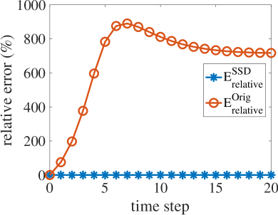
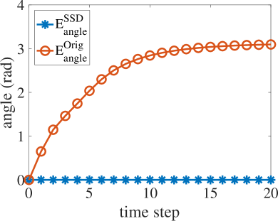
Figure 1: Relative (left) and angle (right) prediction errors on the original and SSD subspaces for system (VIII.1) on a trajectory of length $M=20$.

Example VIII.2

(Duffing Equation): Here, we investigate the efficacy of the proposed methods in approximating Koopman eigenfunctions and invariant subspaces. Consider the Duffing equation [35, Section 4.2]

$$\dot{x}_{1} =x_{2}$$

$$\dot{x}_{2} =-0.5x_{2}+x_{1}-x_{1}^{3},$$ (61)

with state $x^{T}=[x_{1},x_{2}]^{T}$. The system has one unstable equilibrium at the origin and two locally stable equilibria at $[\pm 1,0]^{T}$. We consider the discretized version of (VIII.2) with timestep $\Delta t=0.01s$ and gather $N=5000$ data snapshots uniformly sampled from $\mathcal{M}=[-2,2]\times[-2,2]$. Moreover, we use the dictionary $D$ comprised of all $N_{d}=36$ monomials up to degree 7 in the form of $\prod_{i=1}^{7}y_{i}$, where $y_{i}\in\{1,x_{1},x_{2}\}$. The maximal Koopman-invariant subspace in the span of the dictionary is one dimensional, spanned by the trivial eigenfunction $\phi(x)\equiv 1$. Hence, applying the SSD and SSSD algorithms would result in a trivial solution. Instead, we apply the Approximated-SSD algorithm on the available dictionary snapshots with the accuracy parameter $\epsilon=10^{-3}$. The outcome is the dictionary $\tilde{D}_{\operatorname{aprx}}$ with $\tilde{N}_{d}=15$ elements. We calculate the linear prediction matrix $K^{{\operatorname{SSD}}}_{\operatorname{aprx}}$ using Theorem VII.3. The norm of the perturbation $\|[\Delta_{1}^{*},\Delta_{2}^{*}]\|_{F}$ satisfies

$$\|[\Delta_{1}^{*},\Delta_{2}^{*}]\|_{F}\approx 9.6\times 10^{-4}\|[\tilde{D}_{\operatorname{aprx}}(X),\tilde{D}_{\operatorname{aprx}}(Y)]\|_{F},$$

agreeing with the upper bound provided in Theorem VII.3. We approximate the eigenfunctions of the Koopman operator using the eigendecomposition of $K^{{\operatorname{SSD}}}_{\operatorname{aprx}}$. For space reasons, we only illustrate the leading nontrivial approximated Koopman eigenfunctions with eigenvalue closest to the unit circle. Figure 2(left) shows the real-valued approximated eigenfunction corresponding to the eigenvalue $\lambda=0.9919$. Despite being an approximation, the eigenfunction captures the behavior of the vector field accurately and correctly identifies the attractiveness of the two locally stable equilibria. Given that $|\lambda|<1$, Figure 2(left) predicts that the trajectories eventually converge to one of the stable equilibria. Figure 2(right) shows the absolute value of the approximated Koopman eigenfunctions corresponding to the eigenvalues $\lambda=0.9989\pm 0.0037j$. Similarly to the other plot, it captures information about the shape of the vector field such as the attractive equilibria and their regions of attraction.

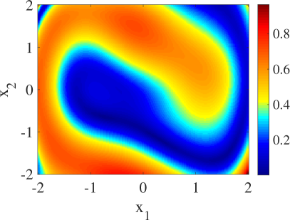
Figure 2: The approximated eigenfunction corresponding to the eigenvalue $\lambda=0.9919$ (left) and the absolute value of the approximated eigenfunctions corresponding to the eigenvalues $\lambda=0.9989\pm 0.0037j$ (right) for the Koopman operator associated with (VIII.2), as identified by the Approximated-SSD algorithm.

We use the relative and angle errors defined in (60) to compare the prediction accuracy of the original dictionary $D$ and the Approximated-SSD dictionary $\tilde{D}_{\operatorname{aprx}}$ (for which we use $K^{{\operatorname{SSD}}}_{\operatorname{aprx}}$). Figure 3 illustrates the relative and angle errors along a trajectory starting from a random initial condition in $[-2,2]\times[-2,2]$ for 30 timesteps. The plot shows the superiority of EDMD over the subspace identified by Approximated-SSD in long-term prediction of dynamical behavior.

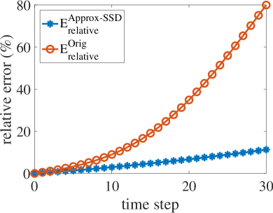
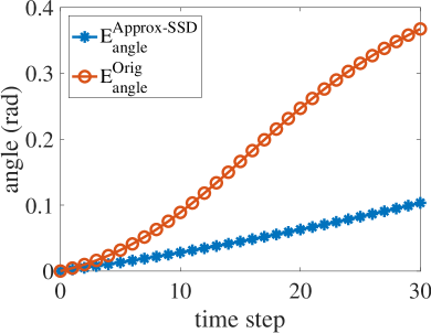
Figure 3: Relative (left) and angle (right) prediction errors on Approximated-SSD and original subspaces for system (VIII.2) on a trajectory of length $M=30$.

IX Conclusions

We have studied the characterization of Koopman-invariant subspaces and Koopman eigenfunctions associated to a dynamical system by means of data-driven methods. We have shown that the application of EDMD over a given dictionary forward and backward in time fully characterizes whether a function evolves linearly in time according to the available data. Building on this result, and under dense sampling, we have established that functions satisfying this condition are Koopman eigenfunctions almost surely. We have developed the SSD algorithm to identify the maximal Koopman-invariant subspace in the span of the given dictionary and formally characterized its correctness. Finally, we have developed extensions to scenarios with large and streaming data sets, where the algorithm refines its output as new data becomes available, and to scenarios where the original dictionary does not contain sufficient informative eigenfunctions, in which case the algorithm obtains instead approximations of the Koopman eigenfunctions and invariant subspaces. Future work will develop parallel and distributed counterparts of the algorithms proposed here over network systems, obtain out-of-sample bounds on prediction accuracy for the output of the Approximated-SSD algorithm, investigate the design of noise-resilient methods to identify Koopman eigenfunctions and invariant subspaces, and explore methods to expand the original dictionary to ensure the existence of non-trivial invariant subspaces.

Here we gather some linear algebraic results.

Lemma .1

(Intersection of Linear Spaces): Let $A,B\in\mathbb{R}^{m\times n}$ be matrices with full column rank. Suppose that the columns of $Z=[(Z^{A})^{T},(Z^{B})^{T}]^{T}\in\mathbb{R}^{2n\times l}$ form a basis for the null space of $[A,B]$, where $Z^{A},Z^{B}\in\mathbb{R}^{n\times l}$. Then,

1. $\mathcal{R}(AZ^{A})=\mathcal{R}(A)\cap\mathcal{R}(B)$;

2. $Z^{A}$ and $Z^{B}$ have full column rank.

Proof:

(a) First, note that $\mathcal{R}(AZ^{A})\subseteq\mathcal{R}(A)$. Moreover, by hypothesis, $[A,B]Z=0$, which leads to $\mathcal{R}(AZ^{A})=\mathcal{R}(BZ^{B})\subseteq\mathcal{R}(B)$. Consequently, $\mathcal{R}(AZ^{A})\subseteq\mathcal{R}(A)\cap\mathcal{R}(B)$. Now, suppose that $v\in\mathcal{R}(A)\cap\mathcal{R}(B)$. By definition, there exist vectors $w_{1},w_{2}\in\mathbb{R}^{n}$ such that $v=Aw_{1}=Bw_{2}$. Then,

$$\begin{bmatrix}A,B\end{bmatrix}\begin{bmatrix}w_{1}\\ -w_{2}\end{bmatrix}=0,$$

which means that $[w_{1}^{T},-w_{2}^{T}]^{T}\in\mathcal{R}(Z)$ and there exists $r\in\mathbb{R}^{l}$ such that $w_{1}=Z^{A}r$ and $w_{2}=-Z^{B}r$. Therefore, $v=Aw_{1}=AZ^{A}r\in\mathcal{R}(AZ^{A})$. Consequently, $\mathcal{R}(A)\cap\mathcal{R}(B)\subseteq\mathcal{R}(AZ^{A})$ and the claim follows.

(b) We prove this part using contradiction. Suppose that there exists $v\neq 0$ such that $Z^{A}v=0$. Also, since $[A,B]Z=0$, one can conclude that $AZ^{A}v=-BZ^{B}v=0$. Since $B$ has full column rank, we have $Z^{B}v=0$. Hence $Zv=0$, which is a contradiction since the columns of $Z$ are linearly independent. A similar reasoning shows that $Z^{B}$ has full column rank. ∎

Lemma .2

Let $A,C,D$ be matrices of appropriate sizes, with $A$ having full column rank. Then $\mathcal{R}(AC)\subseteq\mathcal{R}(AD)$ if and only if $\mathcal{R}(C)\subseteq\mathcal{R}(D)$.

Proof:

$(\Rightarrow)$: Suppose that $v\in\mathcal{R}(C)$, and hence there exists $w$ such that $v=Cw$. Therefore, $Av=ACw\in\mathcal{R}(AC)$. Since $\mathcal{R}(AC)\subseteq\mathcal{R}(AD)$, one can deduce that there exist $r$ such that $ACw=ADr$, and we get $A(v-Dr)=0$. This leads to $v=Dr\in\mathcal{R}(D)$ since $A$ has full column rank, and hence $\mathcal{R}(C)\subseteq\mathcal{R}(D)$.

$(\Leftarrow)$: Suppose that $v\in\mathcal{R}(AC)$, and hence $v=ACw$ for some $w$. Since $\mathcal{R}(C)\subseteq\mathcal{R}(D)$, there exists $r$ such that $Cw=Dr$. As a result, $v=ACw=ADr$ which leads to the conclusion that $v\in\mathcal{R}(AD)$ and the claim follows. ∎

Lemma .3

Let $A_{1},B_{1}\in\mathbb{R}^{m\times n}$, $A_{2},B_{2}\in\mathbb{R}^{l\times n}$, and $C\in\mathbb{R}^{n\times k}$ with $A_{1},B_{1},C$ having full column rank. If

$$\mathcal{R}\Bigg{(}\begin{bmatrix}A_{1}\\ A_{2}\end{bmatrix}\Bigg{)} =\mathcal{R}\Bigg{(}\begin{bmatrix}B_{1}\\ B_{2}\end{bmatrix}\Bigg{)},\quad$$ (62a)

$$\mathcal{R}(A_{1}C) =\mathcal{R}(B_{1}C),$$ (62b)

then

$$\mathcal{R}\Bigg{(}\begin{bmatrix}A_{1}\\ A_{2}\end{bmatrix}C\Bigg{)} =\mathcal{R}\Bigg{(}\begin{bmatrix}B_{1}\\ B_{2}\end{bmatrix}C\Bigg{)}.$$

Proof:

Based on (62a), one can deduce that there exists a nonsingular square matrix $K$ such that

$$A_{1}=B_{1}K,$$ (63a)

$$A_{2}=B_{2}K.$$ (63b)

Multiplying both sides of (63a) by $C$ gives

$$A_{1}C=B_{1}KC.$$ (64)

Moreover, based on (62b), one can deduce that there exists a nonsingular square matrix $K^{*}$

$$A_{1}C=B_{1}CK^{*}.$$ (65)

By subtracting (65) from (64) and considering the fact that $B_{1}$ has full column rank, one can deduce that

$$CK^{*}=KC.$$ (66)

Now, multiplying both sides of (63b) from the right by $C$ and using (66), one can write $A_{2}C=B_{2}CK^{*}$, which in conjunction with (65) leads to

$$\begin{bmatrix}A_{1}\\ A_{2}\end{bmatrix}C=\begin{bmatrix}B_{1}\\ B_{2}\end{bmatrix}CK^{*},$$

completing the proof. ∎

Lemma .4

Let $A$, $\{C_{i}\}_{i=1}^{\infty}$, and $\hat{C}$ be matrices of appropriate sizes. Assume that $A$ has full column rank and $\mathcal{R}(\hat{C})=\bigcap_{i=1}^{\infty}\mathcal{R}(C_{i})$. Then $\mathcal{R}(A\hat{C})=\bigcap_{i=1}^{\infty}\mathcal{R}(AC_{i})$.

Proof:

First, we prove that $\mathcal{R}(A\hat{C})\subseteq\bigcap_{i=1}^{\infty}\mathcal{R}(AC_{i})$. Let $v\in\mathcal{R}(A\hat{C})$, then there exists a vector $w$ such that $v=A\hat{C}w=Ar$, with $r=\hat{C}w$. Note that $r\in\mathcal{R}(\hat{C})$ and consequently $r\in\mathcal{R}(C_{i})$ for all $i\in\mathbb{N}$. Hence, for every $i\in\mathbb{N}$ there exists $z_{i}$ such that $r=C_{i}z_{i}$. Based on the definition of $v$, we have $v=Ar=AC_{i}z_{i}$ for every $i\in\mathbb{N}$. As a result, $v\in\bigcap_{i=1}^{\infty}\mathcal{R}(AC_{i})$ which concludes the proof of this inclusion.

Now, we prove that $\bigcap_{i=1}^{\infty}\mathcal{R}(AC_{i})\subseteq\mathcal{R}(A\hat{C})$. Let $v\in\bigcap_{i=1}^{\infty}\mathcal{R}(AC_{i})$. Then for every $i\in\mathbb{N}$, there exists $w_{i}$ such that $v=AC_{i}w_{i}$. Moreover, $v\in\mathcal{R}(A)$ and since $A$ has full column rank, there exists a unique $r$ such that $v=Ar$. Therefore, for all $i\in\mathbb{N}$, we have $r=C_{i}w_{i}$. Thus, $r\in\bigcap_{i=1}^{\infty}\mathcal{R}(C_{i})$ and consequently, $r\in\mathcal{R}(\hat{C})$. Since $v=Ar$, we have $v\in\mathcal{R}(A\hat{C})$, concluding the proof. ∎

Masih Haseli was born in Kermanshah, Iran in 1991. He received the B.Sc. degree, in 2013, and M.Sc. degree, in 2015, both in Electrical Engineering from Amirkabir University of Technology (Tehran Polytechnic), Tehran, Iran. In 2017, he joined the University of California, San Diego to pursue the Ph.D. degree in Mechanical and Aerospace Engineering. His research interests include system identification, nonlinear systems, network systems, data-driven modeling and control, and distributed and parallel computing. Mr. Haseli was the recipient of the bronze medal in Iran’s national mathematics competition in 2014.

Jorge Cortés (M’02, SM’06, F’14) received the Licenciatura degree in mathematics from Universidad de Zaragoza, Zaragoza, Spain, in 1997, and the Ph.D. degree in engineering mathematics from Universidad Carlos III de Madrid, Madrid, Spain, in 2001. He held postdoctoral positions with the University of Twente, Twente, The Netherlands, and the University of Illinois at Urbana-Champaign, Urbana, IL, USA. He was an Assistant Professor with the Department of Applied Mathematics and Statistics, University of California, Santa Cruz, CA, USA, from 2004 to 2007. He is currently a Professor in the Department of Mechanical and Aerospace Engineering, University of California, San Diego, CA, USA. He is the author of Geometric, Control and Numerical Aspects of Nonholonomic Systems (Springer-Verlag, 2002) and co-author (together with F. Bullo and S. Martínez) of Distributed Control of Robotic Networks (Princeton University Press, 2009). He is a Fellow of IEEE and SIAM. His current research interests include distributed control and optimization, network science, resource-aware control, nonsmooth analysis, reasoning and decision making under uncertainty, network neuroscience, and multi-agent coordination in robotic, power, and transportation networks.

References

- [1] M. Haseli and J. Cortés, “Efficient identification of linear evolutions in nonlinear vector fields: Koopman invariant subspaces,” in IEEE Conf. on Decision and Control, Nice, France, Dec. 2019, pp. 1746–1751.
- [2] B. O. Koopman, “Hamiltonian systems and transformation in Hilbert space,” Proceedings of the National Academy of Sciences, vol. 17, no. 5, pp. 315–318, 1931.
- [3] B. O. Koopman and J. V. Neumann, “Dynamical systems of continuous spectra,” Proceedings of the National Academy of Sciences, vol. 18, no. 3, pp. 255–263, 1932.
- [4] I. Mezić, “Spectral properties of dynamical systems, model reduction and decompositions,” Nonlinear Dynamics, vol. 41, no. 1-3, pp. 309–325, 2005.
- [5] C. W. Rowley, I. Mezić, S. Bagheri, P. Schlatter, and D. S. Henningson, “Spectral analysis of nonlinear flows,” Journal of Fluid Mechanics, vol. 641, pp. 115–127, 2009.
- [6] M. Budišić, R. Mohr, and I. Mezić, “Applied Koopmanism,” Chaos, vol. 22, no. 4, p. 047510, 2012.
- [7] A. Surana, M. O. Williams, M. Morari, and A. Banaszuk, “Koopman operator framework for constrained state estimation,” in IEEE Conf. on Decision and Control, Melbourne, Australia, 2017, pp. 94–101.
- [8] M. Netto and L. Mili, “A robust data-driven Koopman Kalman filter for power systems dynamic state estimation,” IEEE Transactions on Power Systems, vol. 33, no. 6, pp. 7228–7237, 2018.
- [9] A. Mauroy and J. Goncalves, “Koopman-based lifting techniques for nonlinear systems identification,” IEEE Transactions on Automatic Control, vol. 65, no. 6, pp. 2550–2565, 2020.
- [10] D. Bruder, C. D. Remy, and R. Vasudevan, “Nonlinear system identification of soft robot dynamics using Koopman operator theory,” in IEEE Int. Conf. on Robotics and Automation, Montreal, Canada, May 2019, pp. 6244–6250.
- [11] B. Kramer, P. Grover, P. Boufounos, S. Nabi, and M. Benosman, “Sparse sensing and DMD-based identification of flow regimes and bifurcations in complex flows,” SIAM Journal on Applied Dynamical Systems, vol. 16, no. 2, pp. 1164–1196, 2017.
- [12] S. Sinha, U. Vaidya, and R. Rajaram, “Operator theoretic framework for optimal placement of sensors and actuators for control of nonequilibrium dynamics,” Journal of Mathematical Analysis and Applications, vol. 440, no. 2, pp. 750–772, 2016.
- [13] S. Klus, F. Nüske, P. Koltai, H. Wu, I. Kevrekidis, C. Schütte, and F. Noé, “Data-driven model reduction and transfer operator approximation,” Journal of Nonlinear Science, vol. 28, no. 3, pp. 985–1010, 2018.
- [14] A. Alla and J. N. Kutz, “Nonlinear model order reduction via dynamic mode decomposition,” SIAM Journal on Scientific Computing, vol. 39, no. 5, pp. B778–B796, 2017.
- [15] M. Korda and I. Mezić, “Linear predictors for nonlinear dynamical systems: Koopman operator meets model predictive control,” Automatica, vol. 93, pp. 149–160, 2018.
- [16] H. Arbabi, M. Korda, and I. Mezic, “A data-driven Koopman model predictive control framework for nonlinear flows,” arXiv preprint arXiv:1804.05291, 2018.
- [17] S. Peitz and S. Klus, “Koopman operator-based model reduction for switched-system control of PDEs,” Automatica, vol. 106, pp. 184–191, 2019.
- [18] B. Huang, X. Ma, and U. Vaidya, “Feedback stabilization using Koopman operator,” in IEEE Conf. on Decision and Control, Miami Beach, FL, Dec. 2018, pp. 6434–6439.
- [19] E. Kaiser, J. N. Kutz, and S. L. Brunton, “Data-driven discovery of Koopman eigenfunctions for control,” arXiv preprint arXiv:1707.01146, 2017.
- [20] A. Sootla and D. Ernst, “Pulse-based control using Koopman operator under parametric uncertainty,” IEEE Transactions on Automatic Control, vol. 63, no. 3, pp. 791–796, 2017.
- [21] A. Narasingam and J. S. Kwon, “Data-driven feedback stabilization of nonlinear systems: Koopman-based model predictive control,” arXiv preprint arXiv:2005.09741, 2020.
- [22] G. Mamakoukas, M. Castano, X. Tan, and T. Murphey, “Local Koopman operators for data-driven control of robotic systems,” in Robotics: Science and Systems, Freiburg, Germany, Jun. 2019.
- [23] M. L. Castaño, A. Hess, G. Mamakoukas, T. Gao, T. Murphey, and X. Tan, “Control-oriented modeling of soft robotic swimmer with Koopman operators,” in IEEE/ASME International Conference on Advanced Intelligent Mechatronics (AIM), 2020, pp. 1679–1685.
- [24] A. Mauroy and I. Mezić, “Global stability analysis using the eigenfunctions of the Koopman operator,” IEEE Transactions on Automatic Control, vol. 61, no. 11, pp. 3356–3369, 2016.
- [25] P. J. Schmid, “Dynamic mode decomposition of numerical and experimental data,” Journal of Fluid Mechanics, vol. 656, pp. 5–28, 2010.
- [26] K. K. Chen, J. H. Tu, and C. W. Rowley, “Variants of dynamic mode decomposition: boundary condition, Koopman, and Fourier analyses,” Journal of Nonlinear Science, vol. 22, no. 6, pp. 887–915, 2012.
- [27] J. H. Tu, C. W. Rowley, D. M. Luchtenburg, S. L. Brunton, and J. N. Kutz, “On dynamic mode decomposition: theory and applications,” Journal of Computational Dynamics, vol. 1, no. 2, pp. 391–421, 2014.
- [28] M. S. Hemati, M. O. Williams, and C. W. Rowley, “Dynamic mode decomposition for large and streaming datasets,” Physics of Fluids, vol. 26, no. 11, p. 111701, 2014.
- [29] H. Zhang, C. W. Rowley, E. A. Deem, and L. N. Cattafesta, “Online dynamic mode decomposition for time-varying systems,” SIAM Journal on Applied Dynamical Systems, vol. 18, no. 3, pp. 1586–1609, 2019.
- [30] S. Anantharamu and K. Mahesh, “A parallel and streaming dynamic mode decomposition algorithm with finite precision error analysis for large data,” Journal of Computational Physics, vol. 380, pp. 355–377, 2019.
- [31] S. T. M. Dawson, M. S. Hemati, M. O. Williams, and C. W. Rowley, “Characterizing and correcting for the effect of sensor noise in the dynamic mode decomposition,” Experiments in Fluids, vol. 57, no. 3, p. 42, 2016.
- [32] M. S. Hemati, C. W. Rowley, E. A. Deem, and L. N. Cattafesta, “De-biasing the dynamic mode decomposition for applied Koopman spectral analysis of noisy datasets,” Theoretical and Computational Fluid Dynamics, vol. 31, no. 4, pp. 349–368, 2017.
- [33] M. R. Jovanović, P. J. Schmid, and J. W. Nichols, “Sparsity-promoting dynamic mode decomposition,” Physics of Fluids, vol. 26, no. 2, p. 024103, 2014.
- [34] S. L. Clainche and J. M. Vega, “Higher-order dynamic mode decomposition,” SIAM Journal on Applied Dynamical Systems, vol. 16, no. 2, pp. 882–925, 2017.
- [35] M. O. Williams, I. G. Kevrekidis, and C. W. Rowley, “A data-driven approximation of the Koopman operator: Extending dynamic mode decomposition,” Journal of Nonlinear Science, vol. 25, no. 6, pp. 1307–1346, 2015.
- [36] M. Korda and I. Mezić, “On convergence of extended dynamic mode decomposition to the Koopman operator,” Journal of Nonlinear Science, vol. 28, no. 2, pp. 687–710, 2018.
- [37] M. Haseli and J. Cortés, “Approximating the Koopman operator using noisy data: noise-resilient extended dynamic mode decomposition,” in American Control Conference, Philadelphia, PA, Jul. 2019, pp. 5499–5504.
- [38] E. Qian, B. Kramer, B. Peherstorfer, and K. Willcox, “Lift & learn: Physics-informed machine learning for large-scale nonlinear dynamical systems,” Physica D: Nonlinear Phenomena, vol. 406, p. 132401, 2020.
- [39] Q. Li, F. Dietrich, E. M. Bollt, and I. G. Kevrekidis, “Extended dynamic mode decomposition with dictionary learning: A data-driven adaptive spectral decomposition of the Koopman operator,” Chaos, vol. 27, no. 10, p. 103111, 2017.
- [40] N. Takeishi, Y. Kawahara, and T. Yairi, “Learning Koopman invariant subspaces for dynamic mode decomposition,” in Conference on Neural Information Processing Systems, 2017, pp. 1130–1140.
- [41] E. Yeung, S. Kundu, and N. Hodas, “Learning deep neural network representations for Koopman operators of nonlinear dynamical systems,” in American Control Conference, Philadelphia, PA, Jul. 2019, pp. 4832–4839.
- [42] S. E. Otto and C. W. Rowley, “Linearly recurrent autoencoder networks for learning dynamics,” SIAM Journal on Applied Dynamical Systems, vol. 18, no. 1, pp. 558–593, 2019.
- [43] S. L. Brunton, B. W. Brunton, J. L. Proctor, and J. N. Kutz, “Koopman invariant subspaces and finite linear representations of nonlinear dynamical systems for control,” PLOS One, vol. 11, no. 2, pp. 1–19, 2016.
- [44] M. Korda and I. Mezic, “Optimal construction of Koopman eigenfunctions for prediction and control,” IEEE Transactions on Automatic Control, 2020, to appear.
- [45] S. Klus, F. Nüske, S. Peitz, J. H. Niemann, C. Clementi, and C. Schütte, “Data-driven approximation of the Koopman generator: Model reduction, system identification, and control,” arXiv preprint arXiv:1909.10638, 2019.
- [46] G. B. Folland, Real Analysis: Modern Techniques and Their Applications, 2nd ed. New York: Wiley, 1999.
- [47] M. Korda and I. Mezić, “Optimal construction of Koopman eigenfunctions for prediction and control,” 2019. [Online]. Available: https://hal.archives-ouvertes.fr/hal-02278835
- [48] X. Li, S. Wang, and Y. Cai, “Tutorial: Complexity analysis of singular value decomposition and its variants,” arXiv preprint arXiv:1906.12085, 2019.
- [49] L. Mirsky, “Symmetric gauge functions and unitarily invariant norms,” The Quarterly Journal of Mathematics, vol. 11, no. 1, pp. 50–59, 1960.
- [50] I. Markovsky and S. V. Huffel, “Overview of total least-squares methods,” Signal processing, vol. 87, no. 10, pp. 2283–2302, 2007.
- [51] C. Eckart and G. Young, “The approximation of one matrix by another of lower rank,” Psychometrika, vol. 1, no. 3, pp. 211–218, 1936.
- [52] R. M. Jungers and P. Tabuada, “Non-local linearization of nonlinear differential equations via polyflows,” in American Control Conference, Philadelphia, PA, 2019, pp. 1906–1911.