Polarization resolved radiation angular patterns of orientationally ordered nanorods

Abstract

We employ the transfer matrix approach combined with the Green’s function method to theoretically study polarization resolved far-field angular distributions of photoluminescence from quantum nanorods (NRs) embedded in an anisotropic polymer film. The emission and excitation properties of NRs are described by the emission and excitation anisotropy tensors. These tensors and the solution of the emission problem expressed in terms of the evolution operators are used to derive the orientationally averaged coherency matrix of the emitted wavefield. For the case of in-plane alignment and unpolarized excitation, we estimate the emission anisotropy parameter and compute the angular profiles for the photoluminescence polarization parameter such as the degree of linear polarization, the Stokes parameter $s_{1}$, the ellipticity and the polarization azimuth. We show that the alignment order parameter has a profound effect on the angular profiles.

I Introduction

Over the last two decades quantum nanorods (NRs) have been the subject of intense studies as semiconductor nanoheterostructures that possess a unique combination of geometry and size dependent emission and excitation properties Hu et al. (2001); Shabaev and Efros (2004); Talapin et al. (2003); Sitt et al. (2011); Rainó et al. (2012); Vezzoli et al. (2015); Hasegawa et al. (2015); Aubert et al. (2015) (see also a review Krahne et al. (2011)). In addition to quantum confinement effects coming into play at length scales comparable to the bulk exciton Bohr radius, these structures feature linearly polarized photoluminescence Hu et al. (2001) and excitation (absorption) anisotropy Hens and Moreels (2012); Kamal et al. (2012); Angeloni et al. (2016).

The linear polarization of emission is governed by the fine structure of the ground exciton state. It is determined by a number of factors such as the fine structure splittings, the selection rules and the exciton oscillator strengths Efros (1992); Shabaev and Efros (2004); Talapin et al. (2003); Sitt et al. (2011); Krahne et al. (2011); Rainó et al. (2012); Vezzoli et al. (2015). In particular, both excitation and emission of single cadmium selenide (CdSe) quantum rods are found to exhibit strong polarization dependence, indicating that dipole moment exists along the long axis of the rods, e.g., the unique $c$-axis of the wurtzite structure Chen et al. (2001).

There is a variety of applications utilizing the linear polarized emission from the NRs that are used as efficient light emitters for lasing Kazes et al. (2002), biological labeling Yong et al. (2009) and generation of nonclassical light Pisanello et al. (2010). In liquid crystal display devices, it was found that using NRs as backlight source may significantly enhance the optical efficiency of the backlighting system Aubert et al. (2015); Cunningham et al. (2016); Srivastava et al. (2017).

Since the emission and excitation properties of NRs crucially depend on their orientation, it is of paramount importance for any application utilizing the polarized emission from NRs to control and determine their alignment in a film. There are several methods to achieve unidirectional alignment of NRs that have been discussed in the past few years Mohammadimasoudi et al. (2013); Hasegawa et al. (2015); Aubert et al. (2015); Cunningham et al. (2016). One of the most promising approaches uses the photoalignment technique to align NRs in the liquid crystal polymer (LCP) matrix brought in contact with the photoaligning azo-dye layer through the precise control over the orientation of photosensitive dye molecules Du et al. (2015); Schneider et al. (2017).

There are several techniques developed for determination of the three-dimensional (3D) orientation of the transition dipoles of single molecules. These include polarization-sensitive detection of fluorescence through a high-N.A. objective originally proposed in Fourkas (2001) and the methods based on different versions of emission pattern imaging Böhmer and Enderlein (2003); Lieb et al. (2004).

It was demonstrated that far-field polarization microscopy can yield the 3D orientation of CdSe quantum dots Empedocles et al. (1999). In Ref. Lethiec et al. (2014a) it was shown that the 3D orientation of a single fluorescent nanoemitter can be determined by polarization analysis of the emitted light using the model based on the theoretical results obtained in Refs. Lukosz and Kunz (1977a, b); Lukosz (1979, 1981). Results of polarimetric measurements performed on core/shell cadmium selenide/cadmium sulfide (CdSe/CdS) dot-in-rods Lethiec et al. (2014a, b) turned out to be consistent with the hypothesis of a linear dipole tilted with respect to the rod axis. Orientation of gold and rare-earth-doped nanorods was also recently studied in Refs. Wackenhut et al. (2012); Kim et al. (2017).

Angular radiation patterns of nanoemitters such as NRs strongly depend on its orientation. In Ref. Flämmich et al. (2010), orientation of the emissive dipole moments was deduced from measurements of the far-field polarized angular radiation patterns of organic light-emitting diodes (OLED)s in electrical operation. Angular distributions of polarized light from multilayer LED structures studied in Shakya et al. (2005); Schubert et al. (2007); Krames et al. (2007); Matioli and Weisbuch (2011); Yuan et al. (2014) are found to be important for optimization of light extraction efficiency and performance of LED devices.

The radiation patterns of light emitted by NRs, however, have received little attention and are much less studied as compared to the LED systems. In this work, we adapt a systematic approach and theoretically study polarization resolved angular distributions of photoluminescence from NRs embedded in the liquid crystal polymer (LCP) film and aligned by the azo-dye photoaligning layer using the photoalignment technique. This geometry was previously described by Tao Du at al. in Ref. Du et al. (2015).

One of the key features of such a multilayer system is that both the LCP film and the azo-dye layer are optically anisotropic. As it was demonstrated for emission from hyperbolic metamaterials Gu et al. (2014), such an anisotropic environment will profoundly influence angular radiation patterns.

Our theoretical approach to the emission problem developed to analyze the combined effects of NR alignment and optical anisotropy of surrounding media on the angular radiation distributions is based a suitably modified version of the transfer matrix method. We show that this method can be used in combination with the Green’s function technique to obtain our key analytical result giving the orientationally averaged coherency matrix of NR emission expressed in terms of the evolution operators and the orientational averages. The important point is that the coherency matrix also depends on the emission and excitation anisotropy parameters determined by the transition dipole moments, the level populations and the local field screening factors. Our goal is to examine how the angular dependence of the polarization state of emitted light is affected by the orientational ordering, optical anisotropy and the emission/excitation anisotropy parameters.

The paper is organized as follows.

In Sec. II we present our theoretical approach. After introducing the emission and excitation anisotropy tensors in Sec. II.1, we briefly discuss the angular spectrum representation and the evolution operators in Sec. II.2. Necessary details on the transfer matrix method are provided in Sec. II.3. In Sec. II.4, we compute the dyadic Green’s function and solve the single-emitter problem. It is found that the far-field eigenwave amplitudes of the emitted wavefield can be expressed in terms of the evolution operators. The expression for the orientationally averaged coherency matrix of the emitted light is obtained in Sec. II.5. The analytical results are employed to perform numerical analysis of the angular profiles for the polarization characteristics of the emitted light in Sec. III. Finally, in Sec. IV, we draw the results together and make some concluding remarks. Technical details are relegated to Appendix A.

II Theory

II.1 Emission and excitation anisotropy tensors

Semiconductor core/shell nanoheterostructures representing the nanorods (NRs) studied in Ref. Du et al. (2015) are also known as the dot-in-rods where a spherical core is surrounded by a rod-like shell. For the CdSe(cadmium selenide)/CdS (cadmium sulfide) dot-in-rods with adjusted geometry of the hexagonal crystal structures, the wurtzite $c$-axis of both the core and the shell is along the long axis of the rod shell, because the growth process of the shell along the $c$-axis is determined by the crystal anisotropy of the core.

The band-edge exciton fine structure of CdSe nanocrystals consists of eight states with the total angular momentum projection on the $c$-axis $F\in\{0,\pm 1,\pm 2\}$ Efros et al. (1996); Rainó et al. (2012); Vezzoli et al. (2015): $|{\pm 2^{L}}\rangle$, $|{\pm 1^{L,U}}\rangle$ and $|{0^{L,U}}\rangle$, where the superscripts L and U indicate lower and upper sublevels, respectively. There are five bright (dipole allowed) exciton states: $|{\pm 1^{L,U}}\rangle$ and $|{0^{U}}\rangle$. For the state $|{0^{U}}\rangle$, the transition dipole moment $\langle{0}|\mathbf{p}|{0^{U}}\rangle$, where $\mathbf{p}$ is the momentum operator, is directed along the $c$-axis (1D dipole), whereas the transition dipole moments $\langle{0}|\mathbf{p}|{\pm 1^{L,U}}\rangle$ lie in the plane normal to $\hat{\mathbf{c}}$ (2D dipole), where $\hat{\mathbf{c}}$ is the unit vector parallel to the $c$-axis.

For emitted lightwave linearly polarized along the polarization unit vector $\hat{\mathbf{e}}$, the emission probabilities for the bright exciton states are proportional to both the magnitudes of the projections of the transition dipoles on the polarization vector and the populations of the exciton states. So, the polarization dependent factors of the probabilities can be written in the form:

$$N_{0}|\langle{0}|\bigl{(}{\hat{\mathbf{e}}}\cdot{\mathbf{p}}\bigr{)}|{0^{U}}\rangle|^{2}=D_{\parallel}\bigl{(}{\hat{\mathbf{e}}}\cdot{\hat{\mathbf{c}}}\bigr{)}^{2},\quad N_{\pm 1}|\langle{0}|\bigl{(}{\hat{\mathbf{e}}}\cdot{\mathbf{p}}\bigr{)}|{\pm 1^{L,U}}\rangle|^{2}=D_{\perp}^{(L,U)}\left[1-\bigl{(}{\hat{\mathbf{e}}}\cdot{\hat{\mathbf{c}}}\bigr{)}^{2}\right],$$ (1)

where $|{0}\rangle$ stands for the ground state; $N_{0}$ and $N_{\pm 1}$ are the level populations. Formula (1) describes the uniaxial transition anisotropy that leads to the linearly polarized emission. This anisotropy is governed by a number of factors such as the fine structure splittings, the selection rules and the exciton oscillator strengths. Sensitivity of these factors to the size and shape of the nanostructures provides a way to control the optical properties of nanorods Talapin et al. (2003); Shabaev and Efros (2004); Rainó et al. (2012); Vezzoli et al. (2015).

For nanorods embedded in surrounding dielectric media, both the emission and absorption properties of NRs are additionally influenced by the effects of dielectric confinement through the modification of the interactions between charge carriers and the local field effect Rodina and Efros (2016). The latter is the effect of dielectric screening arising from the difference between the external (outside) electric field and the internal local field inside the nanostructures. A systematic theoretical treatment of such screening generally requires using the methods of the effective medium theory (details can be found, e.g., in the monographs Choy (2016); Sihlova (2008)). This theory has been applied to interpret optical properties of nanostructures Hens and Moreels (2012); Kamal et al. (2012); Gordon and Gartstein (2014); Battie et al. (2014); Angeloni et al. (2016); Zhang et al. (2018); Reshetnyak et al. (2018), liquid crystal systems Kiselev et al. (2004); Shelestiuk et al. (2011); Fuh et al. (2013) and hyperbolic metamaterials Kidwai et al. (2012); Zhang and Wu (2015); Li and Khurgin (2016); Zhang and Zhang (2017); Lei et al. (2017).

In the simplest case of cylindrically symmetric and ellipsoidally shaped NRs surrounded by an isotropic dielectric medium, the local field effect can be described in terms of two depolarization factors, $N_{\parallel}$ and $N_{\perp}$, related to the screening factors, $L_{\parallel}=(1+N_{\parallel}(\epsilon_{\mathrm{em}}/\epsilon_{\mathrm{m}}-1))^{-1}$ and $L_{\perp}=(1+N_{\perp}(\epsilon_{\mathrm{em}}/\epsilon_{\mathrm{m}}-1))^{-1}$, where $\epsilon_{\mathrm{m}}$ ($\epsilon_{\mathrm{em}}$) is the dielectric constant of the surrounding medium (NR emitter), for the electric field components directed along and normal to the $c$-axis, respectively. For prolate NRs with sufficiently large aspect ratio, the component along the $c$-axis is characterized by the smallest depolarization factor is $N_{\parallel}$ and, in contrast to the normal components, is almost insensitive to the screening effect.

The local field screening effect can be taken into account by using Eq. (1) with the renormalized transition coefficients: $D_{\parallel}^{(LF)}=D_{\parallel}|L_{\parallel}|^{2}$ and $D_{\perp}^{(LF)}=D_{\perp}|L_{\perp}|^{2}$, where $D_{\perp}=D_{\perp}^{(L)}+D_{\perp}^{(U)}$. Clearly, this effect introduces additional the effective transition anisotropy leading to enhancement of the degree of linear polarization.

In a phenomenological approach, a quantum nanoemitter (NR) is regarded as a point oscillating dipole located at $\mathbf{r}_{\mathrm{em}}$ with the current density $\mathbf{J}_{\mathrm{em}}(\mathbf{r})=\mathbf{J}_{\mathrm{em}}\delta(\mathbf{r}-\mathbf{r}_{\mathrm{em}})$. In this approach, the emission probability and the above transition anisotropy renormalized by the local field effect can be taken into account by replacing the product of the current density amplitudes with the emission dipole tensor averaged over the quantum state of the nanoemitter.

From Eq. (1), this emission anisotropy tensor is uniaxially anisotropic and can be written in the following general form:

$$\langle{{J_{\alpha}^{(\mathrm{em})}[J_{\beta}^{(\mathrm{em})}]}^{\ast}}\rangle_{q}\equiv J_{\alpha\beta}^{(\mathrm{em})}=J_{\perp}^{(\mathrm{em})}\delta_{\alpha\beta}+(J_{\parallel}^{(\mathrm{em})}-J_{\perp}^{(\mathrm{em})})c_{\alpha}c_{\beta}\equiv J_{\mathrm{em}}[\delta_{\alpha\beta}+u_{\mathrm{em}}c_{\alpha}c_{\beta}],$$ (2)

where $\alpha,\beta\in\{x,y,z\}$, $\hat{\mathbf{c}}=(c_{x},c_{y},c_{z})$, $\delta_{\alpha\beta}$ is the Kronecker symbol; an asterisk indicates complex conjugation and $u_{\mathrm{em}}=(J_{\parallel}^{(\mathrm{em})}-J_{\perp}^{(\mathrm{em})})/J_{\perp}^{(\mathrm{em})}$ is the emission anisotropy parameter. The tensor coefficients, $J_{\parallel}^{(\mathrm{em})}$ and $J_{\perp}^{(\mathrm{em})}$, that enter relation (2) are assumed to be proportional to the corresponding renormalized transition coefficients $D_{\parallel}^{(LF)}$ and $D_{\perp}^{(LF)}$.

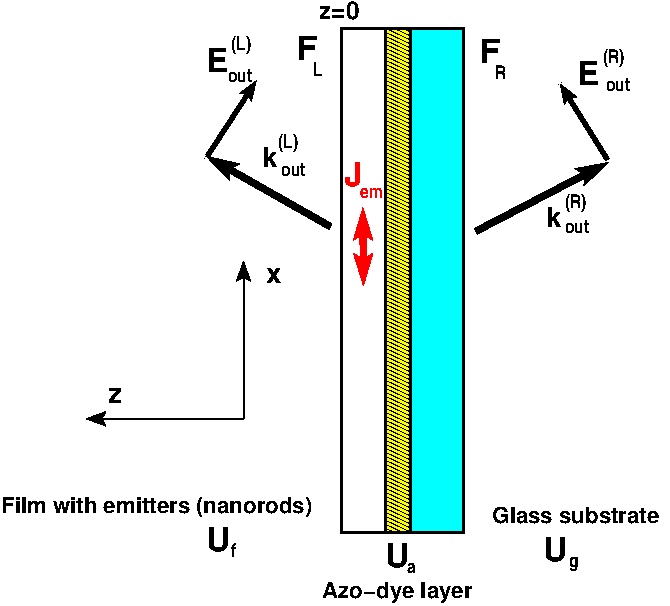
Figure 1: Schematic of emitters embedded in the top layer of the multi-layer structure.

The geometry of our system is schematically depicted in Fig. 1. This system consists of three layers: (a) the film containing the nanorods (emitters) and liquid crystal monomers; (b) the azo-dye photoaligning layer and (c) the glass substrate.

In order to describe light emission from an orientationally ordered ensemble of nanorods we begin with the single-emitter problem. Solution of this problem will yield the expressions for the far-field eigenwave amplitudes $E_{p}^{(\mathrm{em})}$ and $E_{s}^{(\mathrm{em})}$. Then the intensities of the s- and p-polarized waves registered at the detection point are given by

$$I_{p,s}=J_{\mathrm{exc}}(\hat{\mathbf{c}})\langle{|E_{p,s}^{(\mathrm{em})}|^{2}}\rangle_{q}$$ (3)

where $J_{\mathrm{exc}}(\hat{\mathbf{c}})$ is the excitation rate which is proportional to the probability of absorption and depends on the polarization of exciting light. Similar to the emission probability, this dependence is determined by the excitation (absorption) anisotropy tensor

$$J_{\alpha\beta}^{(\mathrm{exc})}=J_{\perp}^{(\mathrm{exc})}\delta_{\alpha\beta}+(J_{\parallel}^{(\mathrm{exc})}-J_{\perp}^{(\mathrm{exc})})c_{\alpha}c_{\beta}\equiv J_{\mathrm{exc}}\left[\delta_{\alpha\beta}+u_{\mathrm{exc}}c_{\alpha}c_{\beta}\right].$$ (4)

So, for the exciting light linear polarized along the unit vector $\hat{\mathbf{e}}_{\mathrm{exc}}$, the excitation rate is given by

$$J_{\mathrm{exc}}(\hat{\mathbf{c}})=J_{\mathrm{exc}}\left[1+u_{\mathrm{exc}}\bigl{(}{\hat{\mathbf{c}}}\cdot{\hat{\mathbf{e}}_{\mathrm{exc}}}\bigr{)}^{2}\right],$$ (5)

where $u_{\mathrm{exc}}=(J_{\parallel}^{(\mathrm{exc})}-J_{\perp}^{(\mathrm{exc})})/J_{\perp}^{(\mathrm{exc})}$ is the excitation anisotropy parameter.

II.2 Operator of evolution

In our subsequent calculations, we shall use the transfer matrix approach which can be regarded as a modified version of the well-known transfer matrix method Markoš and Soukoulis (2008); Yariv and Yeh (2007) and was previously applied to study the polarization-resolved conoscopic patterns of nematic liquid crystal cells Kiselev (2007); Kiselev et al. (2008); Kiselev and Vovk (2010). This approach has also been extended to the case of polarization gratings and used to deduce the general expression for the effective dielectric tensor of deformed helix ferroelectric liquid crystal cells Kiselev et al. (2011); Kiselev and Chigrinov (2014).

In this approach, we deal with a harmonic electromagnetic field characterized by the free-space wave number $k_{\mathrm{vac}}=\omega/c$, where $\omega$ is the frequency (time-dependent factor is $\exp\{-i\omega t\}$), and consider the multi-layer slab geometry shown in Fig. 1. In this geometry, each optically anisotropic layer is sandwiched between the bounding surfaces (substrates) normal to the $z$ axis and is characterized by the dielectric tensor $\epsilon_{ij}$ (in what follows, the magnetic permittivities are equal to unity).

Further, we restrict ourselves to the case of stratified media and use the angular spectrum representation Novotny and Hecht (2006); Mandel and Wolf (1995); Clemmow (1996) of the electromagnetic fields taken in the following form:

$$\{\mathbf{E}(\mathbf{k}_{P},z),\mathbf{H}(\mathbf{k}_{P},z)\}=\int\{\mathbf{E}(\mathbf{r}),\mathbf{H}(\mathbf{r})\}\exp(-i\mathbf{k}_{P}\cdot\mathbf{r}_{P})\mathrm{d}^{2}\mathbf{r}_{P}$$ (6)

where $\mathbf{r}=z\,\hat{\mathbf{z}}+\mathbf{r}_{P}$ and the vector

$$\mathbf{k}_{P}/k_{\mathrm{vac}}=\mathbf{q}_{P}=(q_{x}^{(P)},q_{y}^{(P)},0)=q_{P}(\cos\phi_{P},\sin\phi_{P},0)$$ (7)

represents the lateral component of the wave vector. Then we write down the representation for the electric and magnetic fields, $\mathbf{E}$ and $\mathbf{H}$,

$$\mathbf{E}=E_{z}\hat{\mathbf{z}}+\mathbf{E}_{P},\quad\mathbf{H}=H_{z}\hat{\mathbf{z}}+\hat{\mathbf{z}}\times\mathbf{H}_{P},$$ (8)

where the components directed along the normal to the bounding surface (the $z$ axis) are separated from the tangential (lateral) ones. In this representation, the vectors $\mathbf{E}_{P}=E_{x}\hat{\mathbf{x}}+E_{y}\hat{\mathbf{y}}\equiv\begin{pmatrix}E_{x}\\ E_{y}\end{pmatrix}$ and $\mathbf{H}_{P}=\mathbf{H}\times\hat{\mathbf{z}}\equiv\begin{pmatrix}H_{y}\\ -H_{x}\end{pmatrix}$ are parallel to the substrates and give the lateral components of the electromagnetic field.

We can now substitute the relations (8) into the Maxwell equations

$$\boldsymbol{\nabla}\times\mathbf{E}=i\mu k_{\mathrm{vac}}\mathbf{H},$$ (9a)

$$\boldsymbol{\nabla}\times\mathbf{H}=-ik_{\mathrm{vac}}\mathbf{D}+\frac{4\pi}{c}\mathbf{J}_{\mathrm{em}},$$ (9b)

where $\mathbf{D}=\boldsymbol{\varepsilon}\cdot\mathbf{E}$ is the electric displacement field; $k_{\mathrm{vac}}=\omega/c$ is the free-space wave number and $\mathbf{J}_{\mathrm{em}}(\mathbf{r})=-i\omega\boldsymbol{\mu}_{\mathrm{em}}\delta(\mathbf{r}-\mathbf{r}_{\mathrm{em}})$ is the current density of the dipole emitter located at $\mathbf{r}=\mathbf{r}_{\mathrm{em}}$, and eliminate the $z$ components of the electric and magnetic fields to obtain equations for the tangential components of the electromagnetic field that can be written in the following $4\times 4$ matrix form Kiselev et al. (2008, 2011) (see also Appendix A):

$$-i\partial_{\tau}\mathbf{F}=\mathbf{M}\cdot\mathbf{F}+\mathbf{F}_{J}\equiv\begin{pmatrix}\mathbf{M}_{11}&\mathbf{M}_{12}\\ \mathbf{M}_{21}&\mathbf{M}_{22}\end{pmatrix}\begin{pmatrix}\mathbf{E}_{P}\\ \mathbf{H}_{P}\end{pmatrix}+\mathbf{F}_{J}(\mathbf{k}_{P})\delta(\tau-\tau_{\mathrm{em}}),\quad\tau\equiv k_{\mathrm{vac}}z,$$ (10)

where $\mathbf{M}$ is the differential propagation matrix and its $2\times 2$ block matrices $\mathbf{M}_{ij}$ are given by

$$\mathbf{M}^{(11)}_{\alpha\beta}=-\epsilon_{zz}^{-1}q_{\alpha}^{(P)}\epsilon_{z\beta},\quad\mathbf{M}^{(22)}_{\alpha\beta}=-\epsilon_{zz}^{-1}\epsilon_{\alpha z}q_{\beta}^{(P)},$$ (11a)

$$\mathbf{M}^{(12)}_{\alpha\beta}=\mu\delta_{\alpha\beta}-\frac{q_{\alpha}^{(P)}q_{\beta}^{(P)}}{\epsilon_{zz}},$$ (11b)

$$\mathbf{M}^{(21)}_{\alpha\beta}=\epsilon_{\alpha\beta}-\frac{\epsilon_{\alpha z}\epsilon_{z\beta}}{\epsilon_{zz}}-\mu^{-1}p_{\alpha}^{(P)}p_{\beta}^{(P)},\quad\mathbf{p}_{P}=\hat{\mathbf{z}}\times\mathbf{q}_{P}.$$ (11c)

The last term on the right hand side of Eq. (10)

$$\mathbf{F}_{J}(\mathbf{k}_{P})=\begin{pmatrix}-\mathbf{q}_{P}\epsilon_{zz}^{-1}J_{z}(\mathbf{k}_{P})\\ \mathbf{J}_{P}(\mathbf{k}_{P})-\boldsymbol{\epsilon}_{z}^{\,\prime}\,\epsilon_{zz}^{-1}J_{z}(\mathbf{k}_{P})\end{pmatrix}$$ (12)

is expressed in terms of the Fourier amplitude of the emitter current density

$$\mathbf{J}(\mathbf{k}_{P},\tau)=\frac{4\pi}{c}\int\mathbf{J}_{\mathrm{em}}(\mathbf{r}_{P},z)\mathrm{e}^{-i{\mathbf{k}_{P}}\cdot{\mathbf{r}_{P}}}\mathrm{d}^{2}\mathbf{r}_{P}=\mathbf{J}(\mathbf{k}_{P})\delta(\tau-\tau_{\mathrm{em}}),\quad\tau_{\mathrm{em}}\equiv k_{\mathrm{vac}}z_{\mathrm{em}},$$ (13)

where

$$\mathbf{J}(\mathbf{k}_{P})=-4\pi i\boldsymbol{\mu}_{\mathrm{em}}k_{\mathrm{vac}}\mathrm{e}^{-i{\mathbf{k}_{P}}\cdot{\mathbf{r}_{\mathrm{em}}}}=J_{z}(\mathbf{k}_{P})\hat{\mathbf{z}}+\mathbf{J}_{P}(\mathbf{k}_{P}).$$ (14)

At $\mathbf{F}_{J}=\mathbf{0}$, general solution of the homogeneous system (10)

$$\mathbf{F}(\tau)=\mathbf{U}(\tau,\tau_{0})\cdot\mathbf{F}(\tau_{0})$$ (15)

can be conveniently expressed in terms of the evolution operator which is also known as the propagator and is defined as the matrix solution of the initial value problem

$$-i\partial_{\tau}\mathbf{U}(\tau,\tau_{0}) =\mathbf{M}(\tau)\cdot\mathbf{U}(\tau,\tau_{0}),$$ (16a)

$$\mathbf{U}(\tau_{0},\tau_{0}) =\mathbf{I}_{4},$$ (16b)

where $\mathbf{I}_{n}$ is the $n\times n$ identity matrix. Basic properties of the evolution operator are discussed in Appendix A of Ref. Kiselev and Chigrinov (2014).

For uniformly anisotropic planar structures with the dielectric tensor of the form:

$$\epsilon_{ij}=\epsilon_{z}\delta_{ij}+(\epsilon_{\parallel}-\epsilon_{z})m_{i}m_{j}+(\epsilon_{\perp}-\epsilon_{z})l_{i}l_{j},$$ (17)

where the optical axes

$$\hat{\mathbf{m}}=(m_{x},m_{y},m_{z})=(\cos\psi,\sin\psi,0),\quad\hat{\mathbf{l}}=\hat{\mathbf{z}}\times\hat{\mathbf{m}}=(-\sin\psi,\cos\psi,0)$$ (18)

lie in the plane of substrates (the $x$-$y$ plane), the diagonal block-matrices, $\mathbf{M}_{11}$ and $\mathbf{M}_{22}$, vanish, and nondiagonal block-matrices are given by

$$\mathbf{M}_{12}=\begin{pmatrix}1-q_{P}^{2}/n_{z}^{2}&0\\ 0&1\end{pmatrix},$$ (19)

$$\mathbf{M}_{21}=n_{o}^{2}\begin{pmatrix}1-u_{a}m_{x}^{2}&-u_{a}m_{x}m_{y}\\ -u_{a}m_{x}m_{y}&1-u_{a}m_{y}^{2}-q_{P}^{2}/n_{o}^{2}\end{pmatrix},$$ (20)

where $\mathbf{q}_{P}=q_{P}\hat{\mathbf{x}}$; $n_{z}=\sqrt{\epsilon_{z}}$ and $n_{o}=\sqrt{\epsilon_{\perp}}$ are the principal refractive indices; $u_{a}=(\epsilon_{\parallel}-\epsilon_{\perp})/\epsilon_{\perp}$ is the parameter of in-plane anisotropy. In this case, the operator of evolution can be expressed in terms of the eigenvalue and eigenvector matrices, $\mathbf{\Lambda}\equiv\mathop{\rm diag}\nolimits(\lambda_{1},\lambda_{3},\lambda_{3},\lambda_{4})$ and $\mathbf{V}$, as follows

$$\mathbf{U}(\tau,\tau_{0})=\exp\{i\mathbf{M}\,(\tau-\tau_{0})\}=\mathbf{V}\exp\{i\mathbf{\Lambda}\,(\tau-\tau_{0})\}\mathbf{V}^{-1},\quad\mathbf{M}\mathbf{V}=\mathbf{V}\mathbf{\Lambda},$$ (21)

where the eigenvector and eigenvalue matrices are of the following form:

$$\mathbf{V}=\begin{pmatrix}\mathbf{E}&\mathbf{E}\\ \mathbf{H}&-\mathbf{H}\end{pmatrix},\quad\mathbf{\Lambda}=\mathop{\rm diag}\nolimits(\mathbf{Q},-\mathbf{Q}),\quad\mathbf{Q}=\mathop{\rm diag}\nolimits(q_{e},q_{o})$$ (22)

and can be computed from the relations given in Appendix B of Ref. Kiselev and Chigrinov (2014).

II.3 Transfer matrix

In the ambient medium with $\epsilon_{ij}=\epsilon_{\mathrm{m}}\delta_{ij}$, the general solution (15) can be expressed in terms of plane waves propagating along the wave vectors with the tangential component (7). For such waves, the result is given by

$$\mathbf{F}_{\mathrm{m}}(\tau)=\mathbf{V}_{\mathrm{m}}(\mathbf{q}_{P})\begin{pmatrix}\exp\{i\mathbf{Q}_{\mathrm{m}}\,\tau\}&\mathbf{0}\\ \mathbf{0}&\exp\{-i\mathbf{Q}_{\mathrm{m}}\,\tau\}\end{pmatrix}\begin{pmatrix}\mathbf{E}_{+}\\ \mathbf{E}_{-}\end{pmatrix},$$ (23)

$$\mathbf{Q}_{\mathrm{m}}=q_{\mathrm{m}}\,\mathbf{I}_{2},\quad q_{\mathrm{m}}=\sqrt{n_{\mathrm{m}}^{2}-q_{P}^{2}},$$ (24)

where $\mathbf{V}_{\mathrm{m}}(\mathbf{q}_{P})$ is the eigenvector matrix for the ambient medium given by

$$\mathbf{V}_{\mathrm{m}}(\mathbf{q}_{P})=\mathbf{T}_{\mathrm{rot}}(\phi_{P})\mathbf{V}_{\mathrm{m}}=\begin{pmatrix}\mathbf{Rt}(\phi_{P})&\mathbf{0}\\ \mathbf{0}&\mathbf{Rt}(\phi_{P})\end{pmatrix}\begin{pmatrix}\mathbf{E}_{\mathrm{m}}&-\boldsymbol{\sigma}_{3}\mathbf{E}_{\mathrm{m}}\\ \mathbf{H}_{\mathrm{m}}&\boldsymbol{\sigma}_{3}\mathbf{H}_{\mathrm{m}}\\ \end{pmatrix},$$ (25)

$$\mathbf{E}_{\mathrm{m}}=\begin{pmatrix}q_{\mathrm{m}}/n_{\mathrm{m}}&0\\ 0&1\end{pmatrix},\quad\mathbf{H}_{\mathrm{m}}=\begin{pmatrix}n_{\mathrm{m}}&0\\ 0&q_{\mathrm{m}}\end{pmatrix},$$ (26)

$$\mathbf{Rt}(\phi)=\begin{pmatrix}\cos\phi&-\sin\phi\\ \sin\phi&\cos\phi\end{pmatrix},$$ (27)

$\{\boldsymbol{\sigma}_{1},\boldsymbol{\sigma}_{2},\boldsymbol{\sigma}_{3}\}$ are the Pauli matrices

$$\boldsymbol{\sigma}_{1}=\begin{pmatrix}0&1\\ 1&0\end{pmatrix},\>\boldsymbol{\sigma}_{2}=\begin{pmatrix}0&-i\\ i&0\end{pmatrix},\>\boldsymbol{\sigma}_{3}=\begin{pmatrix}1&0\\ 0&-1\end{pmatrix}.$$ (28)

From Eq. (23), the vector amplitudes $\mathbf{E}_{+}$ and $\mathbf{E}_{-}$ correspond to the forward and backward eigenwaves with $\mathbf{k}_{+}=k_{\mathrm{vac}}(q_{\mathrm{m}}\,\hat{\mathbf{z}}+\mathbf{q}_{P})$ and $\mathbf{k}_{-}=k_{\mathrm{vac}}(-q_{\mathrm{m}}\,\hat{\mathbf{z}}+\mathbf{q}_{P})$, respectively. Figure 1 shows that, in the half space $z\geq z_{0}$ after the exit face of the film with embedded emitters $z=z_{0}$, these eigenwaves describe the incoming and outgoing waves

$$\mathbf{E}_{+}|_{z\geq z_{0}}=\mathbf{E}_{\mathrm{out}}^{(L)},\quad\mathbf{E}_{-}|_{z\geq z_{0}}=\mathbf{E}_{\mathrm{in}}^{(L)}=\mathbf{0},$$ (29)

whereas, in the half space $z\leq z_{3}=-D$ before the entrance face of the glass substrate, these waves are given by

$$\mathbf{E}_{+}|_{z\leq z_{3}}=\mathbf{E}_{\mathrm{in}}^{(R)}=\mathbf{0},\quad\mathbf{E}_{-}|_{z\leq z_{3}}=\mathbf{E}_{\mathrm{out}}^{(R)}.$$ (30)

The boundary conditions require the tangential components of the electric and magnetic fields to be continuous at the boundary surfaces of the multi-layer structure:

$$\mathbf{F}_{L}\equiv\mathbf{F}(z_{0})=\mathbf{F}_{\mathrm{m}}(z_{0}+0)=\mathbf{V}_{\mathrm{m}}(\mathbf{q}_{P})\begin{pmatrix}\mathbf{E}_{\mathrm{out}}^{(L)}\\ \mathbf{E}_{\mathrm{in}}^{(L)}\end{pmatrix},$$

$$\mathbf{F}_{R}\equiv\mathbf{F}(z_{3})=\mathbf{F}_{\mathrm{m}}(z_{3}-0)=\mathbf{V}_{\mathrm{m}}(\mathbf{q}_{P})\begin{pmatrix}\mathbf{E}_{\mathrm{in}}^{(R)}\\ \mathbf{E}_{\mathrm{out}}^{(R)}\end{pmatrix}.$$ (31)

In the standard light scattering (transmission/reflection) problem, we can use the boundary conditions (II.3) to rewrite the relation

$$\mathbf{F}_{L}=\mathbf{U}(\tau_{0},\tau_{3})\cdot\mathbf{F}_{R},\quad\tau_{i}=k_{\mathrm{vac}}z_{i},$$ (32)

in the form

$$\begin{pmatrix}\mathbf{E}_{\mathrm{out}}^{(L)}\\ \mathbf{E}_{\mathrm{in}}^{(L)}\end{pmatrix}=\mathbf{T}\begin{pmatrix}\mathbf{E}_{\mathrm{in}}^{(R)}\\ \mathbf{E}_{\mathrm{out}}^{(R)}\end{pmatrix}$$ (33)

and introduce the transfer matrix $\mathbf{T}$ linking the amplitudes of the eigenwaves in the half spaces $z>z_{0}$ and $z<z_{3}$ bounded by the faces of the multilayer structure. This matrix is the evolution operator $\mathbf{U}(\tau_{0},\tau_{3})$ in the basis of eigenmodes of the surrounding medium which is given by

$$\mathbf{T}(\tau_{0},\tau_{3})\equiv\mathbf{T}=\mathbf{V}_{\mathrm{m}}^{-1}(\mathbf{q}_{P})\mathbf{U}(\tau_{0},\tau_{3})\mathbf{V}_{\mathrm{m}}(\mathbf{q}_{P})=\mathbf{V}_{\mathrm{m}}^{-1}\mathbf{U}_{\mathrm{rot}}(\tau_{0},\tau_{3})\mathbf{V}_{\mathrm{m}}=\begin{pmatrix}\mathbf{T}_{11}&\mathbf{T}_{12}\\ \mathbf{T}_{21}&\mathbf{T}_{22}\end{pmatrix},$$ (34)

where $\mathbf{U}_{\mathrm{rot}}(\tau,\tau_{0})=\mathbf{T}_{\mathrm{rot}}(-\phi_{P})\mathbf{U}(\tau,\tau_{0})\mathbf{T}_{\mathrm{rot}}(\phi_{P})$ is the rotated operator of evolution. This operator is the solution of the initial value problem (16) with $\mathbf{M}(\tau)$ replaced with $\mathbf{M}_{\mathrm{rot}}(\tau)=\mathbf{T}_{\mathrm{rot}}(-\phi_{P})\mathbf{M}(\tau)\mathbf{T}_{\mathrm{rot}}(\phi_{P})$. The scattering matrix relating the amplitudes of the incoming and outgoing waves can be expressed in terms of the block matrices $\mathbf{T}_{ij}$ giving the expressions for the transmission and reflection matrices Kiselev and Chigrinov (2014). We shall need the results for the case where the incident wave $\mathbf{E}_{\mathrm{inc}}=\mathbf{E}_{\mathrm{in}}^{(L)}$ is coming from the half-space $z>z_{0}$:

$$\mathbf{T}_{L}=\mathbf{T}_{22}^{-1},\quad\mathbf{R}_{L}=\mathbf{T}_{12}\mathbf{T}_{22}^{-1},$$ (35)

where $\mathbf{T}_{L}$ and $\mathbf{R}_{L}$ are the transmission and reflection matrices, respectively.

Our concluding remark in this section is that, for the multi-layer structure that consists of three layers depicted in Fig. 1, the evolution operator and the transfer matrix are given by

$$\mathbf{U}(\tau_{0},\tau_{3})=\mathbf{U}_{f}(h_{f})\mathbf{U}_{a}(h_{a})\mathbf{U}_{g}(h_{g}),\quad\mathbf{T}(\tau_{0},\tau_{3})=\mathbf{T}_{f}(h_{f})\mathbf{T}_{a}(h_{a})\mathbf{T}_{g}(h_{g}),$$ (36)

where $\mathbf{U}_{f}(h_{f})=\mathbf{U}_{f}(\tau_{0},\tau_{1})$ is the evolution operator for the film containing the nanorods, $D_{f}$ is the film thickness ($h_{f}=k_{\mathrm{vac}}D_{f}$); $\mathbf{U}_{a}(h_{a})=\mathbf{U}_{a}(\tau_{1},\tau_{2})$ is the evolution operator for the azo-dye layer, $D_{a}$ is the layer thickness ($h_{a}=k_{\mathrm{vac}}D_{a}$); $\mathbf{U}_{g}(h_{g})=\mathbf{U}_{a}(\tau_{2},\tau_{3})$ is the evolution operator for the glass substrate, $D_{g}$ is the thickness of the substrate ($h_{g}=k_{\mathrm{vac}}D_{g}$).

II.4 Dyadic Green’s function and emission problem

At $\mathbf{F}_{J}(\mathbf{k}_{P})\neq\mathbf{0}$, the solution of non-homogeneous system

$$\mathbf{F}_{\mathrm{em}}(\tau)=\mathbf{G}(\tau)\mathbf{F}_{J}(\mathbf{k}_{P})$$ (37)

describing light radiation of the dipole emitter is expressed in terms of the dyadic (matrix-valued) Green’s function $\mathbf{G}(\tau)$ that can be found by solving the following equation

$$-i\partial_{\tau}\mathbf{G}=\mathbf{M}\cdot\mathbf{G}+\mathbf{I}_{4}\delta(\tau-\tau_{\mathrm{em}}).$$ (38)

For uniformly anisotropic layer with the propagator given by Eqs. (21) and (22), we can use the Fourier transform technique combined with the residue calculus (the poles at $q_{o,e}$ are shifted to the upper half of the complex plane: $q_{o,e}\to q_{o,e}+i\delta_{+}$) to obtain the following expression for the Green’s function:

$$\mathbf{G}(\tau)=i\mathbf{V}\begin{pmatrix}H(\tau-\tau_{\mathrm{em}})\mathrm{e}^{i\mathbf{Q}(\tau-\tau_{\mathrm{em}})}&\mathbf{0}\\ \mathbf{0}&-H(\tau_{\mathrm{em}}-\tau)\mathrm{e}^{-i\mathbf{Q}(\tau-\tau_{\mathrm{em}})}\end{pmatrix}\mathbf{V}^{-1},$$ (39)

where $H(\tau)=\begin{cases}1,&\tau>0\\ 1/2,&\tau=0\\ 0,&\tau<0\end{cases}$ is the Heaviside step function.

So, the electromagnetic field inside the film where $\tau_{1}\leq\tau\leq\tau_{0}$ is given by

$$\mathbf{F}_{f}(\tau)=\mathbf{U}_{f}(\tau,\tau_{1})\mathbf{F}_{0}+\mathbf{F}_{\mathrm{em}}(\tau),$$ (40)

where the first term on the right hand side (general solution of the homogeneous system written in the form given by Eq. (15)) represents the waves reflected from (and transmitted through) the boundaries of the film. The continuity conditions at the film boundaries $\tau=\tau_{0}$ and $\tau=\tau_{1}$ are

$$\mathbf{F}_{f}(\tau_{0})=\mathbf{F}_{L},\quad\mathbf{F}_{f}(\tau_{1})=\mathbf{U}_{a}(h_{a})\mathbf{U}_{g}(h_{g})\mathbf{F}_{R}.$$ (41)

After eliminating $\mathbf{F}_{0}$ from Eq. (41), we have

$$\mathbf{F}_{L}-\mathbf{U}(\tau_{0},\tau_{3})\mathbf{F}_{R}=\mathbf{F}_{\mathrm{em}}(\tau_{0})-\mathbf{U}_{f}(\tau_{0},\tau_{1})\mathbf{F}_{\mathrm{em}}(\tau_{1})$$

$$=[\mathbf{G}(\tau_{0})-\mathbf{U}_{f}(\tau_{0},\tau_{1})\mathbf{G}(\tau_{1})]\mathbf{F}_{J}.$$ (42)

For the Green’s function given in Eq. (39), the relation (II.4) can be further simplified with the help of the identity

$$\mathbf{G}(\tau_{0})-\mathbf{U}_{f}(\tau_{0},\tau_{1})\mathbf{G}(\tau_{1})=i\mathop{\rm sign}\nolimits(\tau_{0}-\tau_{\mathrm{em}})\mathbf{U}_{f}(\tau_{0},\tau_{\mathrm{em}}).$$ (43)

We can now use Eqs. (29)– (32) to express the result in terms of the eigenwave amplitudes $\mathbf{E}_{\mathrm{out}}^{(L)}$ and $\mathbf{E}_{\mathrm{out}}^{(R)}$ as follows

$$\begin{pmatrix}\mathbf{E}_{\mathrm{out}}^{(L)}\\ \mathbf{0}\end{pmatrix}-\mathbf{T}\begin{pmatrix}\mathbf{0}\\ \mathbf{E}_{\mathrm{out}}^{(R)}\end{pmatrix}=\mathbf{T}_{\mathrm{em}}\begin{pmatrix}\mathbf{J}_{H}\\ \mathbf{J}_{E}\end{pmatrix},$$ (44)

$$\mathbf{T}_{\mathrm{em}}=i\mathbf{T}_{f}(\tau_{0},\tau_{\mathrm{em}})\mathbf{V}_{\mathrm{m}}^{-1}=\frac{i}{2\pi k_{\mathrm{vac}}q_{\mathrm{m}}}\begin{pmatrix}\mathbf{T}_{11}^{(\mathrm{em})}&\mathbf{T}_{12}^{(\mathrm{em})}\\ \mathbf{T}_{21}^{(\mathrm{em})}&\mathbf{T}_{22}^{(\mathrm{em})}\end{pmatrix},$$ (45)

where $q_{\mathrm{m}}/n_{\mathrm{m}}$ is the $z$-component of the unit wave vector $\hat{\mathbf{k}}_{+}=\mathbf{k}_{+}/n_{\mathrm{m}}k_{\mathrm{vac}}$; $\mathbf{J}_{H}$ and $\mathbf{J}_{E}$ are given by

$$\mathbf{J}_{H}=-\frac{q_{P}}{\epsilon_{zz}}J_{z}\begin{pmatrix}1\\ 0\end{pmatrix},\quad\mathbf{J}_{E}=\mathbf{Rt}(-\phi_{P})\mathbf{J}_{P}.$$ (46)

In our final step, we deduce the expressions for the far-field amplitudes of the emitted (outgoing) waves, $\mathbf{E}_{L}^{(f-f)}$ and $\mathbf{E}_{R}^{(f-f)}$ from Eq. (44). The far-field asymptotic behavior of the amplitudes in a fixed direction $\hat{\mathbf{r}}=\mathbf{r}/r$ is known Mandel and Wolf (1995); Novotny and Hecht (2006) to be determined by the plane wave amplitude of the angular spectrum representation with $\hat{\mathbf{k}}_{+}=\hat{\mathbf{r}}$. So, the far-field amplitudes of the radiated waves, $\mathbf{E}_{L}^{(f-f)}$ and $\mathbf{E}_{R}^{(f-f)}$, are proportional to $\mathbf{E}_{\mathrm{out}}^{(L)}$ and $\mathbf{E}_{\mathrm{out}}^{(R)}$ multiplied by the $z$-component of $\mathbf{k}_{+}=k_{\mathrm{vac}}q_{\mathrm{m}}\hat{\mathbf{z}}+\mathbf{k}_{P}$ and $\mathbf{k}_{-}=-k_{\mathrm{vac}}q_{\mathrm{m}}\hat{\mathbf{z}}+\mathbf{k}_{P}$, respectively. The result reads

$$\mathbf{E}_{\mathrm{em}}=\begin{pmatrix}E_{p}^{(\mathrm{em})}\\ E_{s}^{(\mathrm{em})}\end{pmatrix}\equiv\mathbf{E}_{L}^{(f-f)}=-2\pi ik_{\mathrm{vac}}q_{\mathrm{m}}\mathbf{E}_{\mathrm{out}}^{(L)}=\mathbf{W}_{H}\mathbf{J}_{H}+\mathbf{W}_{E}\mathbf{J}_{E},$$ (47)

$$\mathbf{W}_{H}=\mathbf{T}_{11}^{(\mathrm{em})}-\mathbf{R}_{L}\mathbf{T}_{21}^{(\mathrm{em})},\quad\mathbf{W}_{E}=\mathbf{T}_{12}^{(\mathrm{em})}-\mathbf{R}_{L}\mathbf{T}_{22}^{(\mathrm{em})},$$ (48)

$$\mathbf{E}_{R}^{(f-f)}=2\pi ik_{\mathrm{vac}}q_{\mathrm{m}}\mathbf{E}_{\mathrm{out}}^{(R)}=\mathbf{T}_{L}(\mathbf{T}_{21}^{(\mathrm{em})}\mathbf{J}_{H}+\mathbf{T}_{22}^{(\mathrm{em})}\mathbf{J}_{E}),$$ (49)

where the reflection and the transmission matrices, $\mathbf{R}_{L}$ and $\mathbf{T}_{L}$, are defined in Eq. (35). In what follows, the emitted wavefield (47) will be our primary concern.

II.5 Orientational averaging

We shall assume that an ensemble of aligned NRs can be treated as a collection of incoherently emitting and differently oriented dipoles and the total intensity of the emitters is a sum of the intensities. Orientation of a nanorod is specified by the tilt and azimuthal angles, $\theta_{c}$ and $\phi_{c}$, giving the direction of the $c$-axis: $\hat{\mathbf{c}}=(\cos\theta_{c}\cos\phi_{c},\cos\theta_{c}\sin\phi_{c},\sin\theta_{c})$ and the total intensities of the p- and s-waves can be obtained by averaging the intensities given in Eq. (3) over orientation of the $c$-axis.

More generally, the emitted wavefield can be described by the coherency matrix Mandel and Wolf (1995); Born and Wolf (1999)

$$\mathbf{M}=\langle{J_{\mathrm{exc}}(\hat{\mathbf{c}})\mathbf{E}_{\mathrm{em}}\otimes{\mathbf{E}}^{\ast}_{\mathrm{em}}}\rangle=\begin{pmatrix}\langle{J_{\mathrm{exc}}(\hat{\mathbf{c}})\langle{|E_{p}^{(\mathrm{em})}|^{2}}\rangle_{q}}\rangle_{\hat{\mathbf{c}}}&\langle{J_{\mathrm{exc}}(\hat{\mathbf{c}})\langle{E_{p}^{(\mathrm{em})}{[E_{s}^{(\mathrm{em})}]}^{\ast}}\rangle_{q}}\rangle_{\hat{\mathbf{c}}}\\ \langle{J_{\mathrm{exc}}(\hat{\mathbf{c}})\langle{E_{s}^{(\mathrm{em})}{[E_{p}^{(\mathrm{em})}]}^{\ast}}\rangle_{q}}\rangle_{\hat{\mathbf{c}}}&\langle{J_{\mathrm{exc}}(\hat{\mathbf{c}})\langle{|E_{s}^{(\mathrm{em})}|^{2}}\rangle_{q}}\rangle_{\hat{\mathbf{c}}}\end{pmatrix},$$ (50)

where an asterisk stands for complex conjugation, can now be calculated using the matrix relations (47) and (48). This matrix is given by

$$\mathbf{M}=\mathbf{W}_{H}\langle{J_{\mathrm{exc}}(\hat{\mathbf{c}})\mathbf{J}_{H}\otimes{\mathbf{J}}^{\ast}_{H}}\rangle{\mathbf{W}}^{\dagger}_{H}+\mathbf{W}_{E}\mathbf{Rt}(-\phi_{P})\langle{J_{\mathrm{exc}}(\hat{\mathbf{c}})\mathbf{J}_{P}\otimes{\mathbf{J}}^{\ast}_{P}}\rangle\mathbf{Rt}(\phi_{P}){\mathbf{W}}^{\dagger}_{E},$$ (51)

$$\langle{J_{\mathrm{exc}}(\hat{\mathbf{c}})\mathbf{J}_{H}\otimes{\mathbf{J}}^{\ast}_{H}}\rangle=\frac{q_{P}^{2}}{\epsilon_{z}^{2}}\begin{pmatrix}1&0\\ 0&0\end{pmatrix}\langle{J_{\mathrm{exc}}(\hat{\mathbf{c}}){J}^{(\mathrm{em})}_{zz}}\rangle_{\hat{\mathbf{c}}},$$ (52)

$$[\langle{J_{\mathrm{exc}}(\hat{\mathbf{c}})\mathbf{J}_{P}\otimes{\mathbf{J}}^{\ast}_{P}}\rangle]_{\alpha\beta}=\langle{J_{\mathrm{exc}}(\hat{\mathbf{c}}){J}^{(\mathrm{em})}_{\alpha\beta}}\rangle_{\hat{\mathbf{c}}},$$ (53)

where a dagger will indicate Hermitian conjugation and $\langle{...}\rangle_{\hat{\mathbf{c}}}$ stands for orientational averages.

The result of orientational averaging is expressed in terms of the two symmetric matrices:

$$\mathbf{C}_{\alpha\beta}^{(e)}=\langle{c_{\alpha}c_{\beta}}\rangle_{\hat{\mathbf{c}}},\quad\mathbf{C}_{\alpha\beta}^{(ex)}=\langle{c_{\mathrm{exc}}^{2}c_{\alpha}c_{\beta}}\rangle_{\hat{\mathbf{c}}},$$ (54)

where $c_{\mathrm{exc}}=\bigl{(}{\hat{\mathbf{c}}}\cdot{\hat{\mathbf{e}}_{\mathrm{exc}}}\bigr{)}$ and $\hat{\mathbf{e}}_{\mathrm{exc}}$ is the polarization unit vector of the exciting light. Orientational ordering is described by the eigenvalues and the eigenvectors (the principal axes) of these matrices. Perfectly in-plane ordering presents the important special case with vanishing tilt angle, $\theta_{c}=0$. We shall, however, consider a more general case with nonvanishing $\theta_{c}$ and assume that the angles are statistically independent and the principal (alignment) axes are directed along the coordinate axes. The latter implies that the matrices (54) are both diagonal. It immediately follows that the matrix (53) is also diagonal

$$\langle{J_{\mathrm{exc}}(\hat{\mathbf{c}})\mathbf{J}_{P}\otimes{\mathbf{J}}^{\ast}_{P}}\rangle=\gamma_{0}\mathbf{I}_{2}+\gamma_{3}\boldsymbol{\sigma}_{3},\quad\langle{J_{\mathrm{exc}}(\hat{\mathbf{c}}){J}^{(\mathrm{em})}_{zz}}\rangle_{\hat{\mathbf{c}}}=\gamma_{z}$$ (55)

and the coherency matrix (51) can be written in the form of a linear combination:

$$\mathbf{M}=J_{\mathrm{em}}J_{\mathrm{exc}}[\gamma_{0}\mathbf{W}_{0}+\gamma_{3}(\cos 2\phi_{P}\mathbf{W}_{3}-\sin 2\phi_{P}\mathbf{W}_{1})+\gamma_{z}\mathbf{W}_{z}],$$ (56a)

$$\mathbf{W}_{0}=\mathbf{W}_{E}{\mathbf{W}}^{\dagger}_{E},\quad\mathbf{W}_{i}=\mathbf{W}_{E}\boldsymbol{\sigma}_{i}{\mathbf{W}}^{\dagger}_{E},\quad\mathbf{W}_{z}=\frac{q_{P}^{2}}{\epsilon_{z}^{2}}\mathbf{W}_{H}\begin{pmatrix}1&0\\ 0&0\end{pmatrix}{\mathbf{W}}^{\dagger}_{H},$$ (56b)

$$\gamma_{0}=1+u_{\mathrm{exc}}\langle{c_{\mathrm{exc}}^{2}}\rangle_{\hat{\mathbf{c}}}+\frac{u_{\mathrm{em}}}{2}\left[\langle{c_{x}^{2}+c_{y}^{2}}\rangle_{\hat{\mathbf{c}}}+u_{\mathrm{exc}}\langle{c_{\mathrm{exc}}^{2}(c_{x}^{2}+c_{y}^{2})}\rangle_{\hat{\mathbf{c}}}\right],$$ (56c)

$$\gamma_{3}=\frac{u_{\mathrm{em}}}{2}\left[\langle{c_{x}^{2}-c_{y}^{2}}\rangle_{\hat{\mathbf{c}}}+u_{\mathrm{exc}}\langle{c_{\mathrm{exc}}^{2}(c_{x}^{2}-c_{y}^{2})}\rangle_{\hat{\mathbf{c}}}\right],$$ (56d)

$$\gamma_{z}=1+u_{\mathrm{exc}}\langle{c_{\mathrm{exc}}^{2}}\rangle_{\hat{\mathbf{c}}}+u_{\mathrm{em}}\left[\langle{c_{z}^{2}}\rangle_{\hat{\mathbf{c}}}+u_{\mathrm{exc}}\langle{c_{\mathrm{exc}}^{2}c_{z}^{2}}\rangle_{\hat{\mathbf{c}}}\right].$$ (56e)

Orientational averages that enter the coefficients of the linear combination (56a) can be expressed in terms of the orientational parameters characterizing ordering of aligned NRs. For in-plane ordering, these parameters are as follows

$$\langle{\cos^{2}\phi_{c}}\rangle_{\hat{\mathbf{c}}}=\frac{1+p}{2},\quad\langle{\sin^{2}\phi_{c}}\rangle_{\hat{\mathbf{c}}}=\frac{1-p}{2},\quad\langle{\cos^{2}\phi_{c}\sin^{2}\phi_{c}}\rangle_{\hat{\mathbf{c}}}=q,$$ (57)

where $0\leq q\leq\langle{\cos^{2}\phi_{c}}\rangle_{\hat{\mathbf{c}}}\langle{\sin^{2}\phi_{c}}\rangle_{\hat{\mathbf{c}}}=(1-p^{2})/4$ and $-1\leq p\leq 1$ is the in-plane orientational (alignment) order parameter. Similar results for the averages over the tilt angle $\theta_{c}$ characterizing out-of-plane deviations of the $c$-axis are given by

$$\langle{\sin^{2}\theta_{c}}\rangle_{\hat{\mathbf{c}}}=p_{z},\quad\langle{\cos^{2}\theta_{c}}\rangle_{\hat{\mathbf{c}}}=1-p_{z},\quad\langle{\cos^{2}\theta_{c}\sin^{2}\theta_{c}}\rangle_{\hat{\mathbf{c}}}=q_{z},$$ (58)

where $0\leq q_{z}\leq p_{z}(1-p_{z})$ and $0\leq p_{z}\leq 1$ is the out-of-plane order parameter that equals zero in the limiting case of purely in-plane ordering.

In the subsequent section, these general formulas will be used to perform numerical analysis.

III Results

The lightfield emitted by NRs is generally partially polarized and the far-field angular distributions of its polarization parameters are determined by the coherency matrix

$$\mathbf{M}(q_{P},\phi_{P})\equiv\mathbf{M}(\theta,\phi)=\frac{1}{2}\bigl{[}I(\theta,\phi)\mathbf{I}_{2}+S_{1}(\theta,\phi)\boldsymbol{\sigma}_{3}+$$

$$S_{2}(\theta,\phi)\boldsymbol{\sigma}_{1}+S_{3}(\theta,\phi)\boldsymbol{\sigma}_{2}\bigr{]},$$ (59)

$$q_{P}\equiv|\mathbf{k}_{P}|/k_{\mathrm{vac}}=n_{\mathrm{m}}\sin\theta,\quad\phi_{P}\equiv\phi,$$ (60)

where $I(\theta,\phi)=I_{p}(\theta,\phi)+I_{s}(\theta,\phi)=\mathop{\rm Tr}\nolimits\mathbf{M}(\theta,\phi)$ is the total intensity and $\{S_{1},S_{2},S_{3}\}$ are the Stokes parameters, evaluated as a function of the emission (detection) angle, $\theta$, and the azimuthal angle, $\phi=\phi_{P}$, (see Eq. (7)) that specifies orientation of the emission plane ($\phi$ is the angle between the alignment axis and the emission plane). Though the polarization state of partially polarized radiation from nanoemitters such as NRs with the degree of polarization

$$P=\sqrt{s_{1}^{2}+s_{2}^{2}+s_{3}^{2}}=\sqrt{1-\frac{4\det\mathbf{M}}{(\mathop{\rm Tr}\nolimits\mathbf{M})^{2}}},\quad s_{i}\equiv S_{i}(\theta,\phi)/I(\theta,\phi),$$ (61)

can be completely described using the Stokes parameters, there is a number of the technologically important parameters widely used to characterize the anisotropy of photoluminescence.

One of these parameters is the degree of linear polarization

$$DOP=\sqrt{s_{1}^{2}+s_{2}^{2}}=\frac{I_{\mathrm{max}}-I_{\mathrm{min}}}{I_{\mathrm{max}}+I_{\mathrm{min}}}$$ (62)

where $I_{\mathrm{max}}$ and $I_{\mathrm{min}}$ are the maximum and minimum intensities of the curve representing the experimentally measured intensity of light passed through the rotating polarizer placed in the emission beam path. Alternatively, the Stokes parameter

$$s_{1}=\frac{I_{p}-I_{s}}{I_{p}+I_{s}}$$ (63)

and the related polarization ratios

$$R_{ps}=I_{p}/I_{s},\quad R_{sp}=I_{s}/I_{p},$$ (64)

are also used as convenient measures characterizing the anisotropy of emission in terms of the intensities of the p-polarized and s-polarized waves: $I_{p}\equiv I_{p}(\theta,\phi)=\mathbf{M}_{11}(\theta,\phi)$ and $I_{s}\equiv I_{s}(\theta,\phi)=\mathbf{M}_{22}(\theta,\phi)$. Note that the case where the degree of linear polarization is equal to the magnitude of $s_{1}$, $DOP=|s_{1}|$, occurs only when the Stokes parameter $S_{2}=2\mathop{\rm Re}\nolimits\mathbf{M}_{21}$ vanishes and the polarization azimuth of the polarization ellipse

$$\psi_{p}=2^{-1}\arg(s_{1}+is_{2})$$ (65)

differs from zero and $\pi/2$. The ellipticity of the polarization ellipse characterizing the polarized part of emission

$$\epsilon_{\mathrm{ell}}=\tan[2^{-1}\arcsin(s_{3}/P)]$$ (66)

is expressed in terms of the Stokes parameter $S_{3}=2\mathop{\rm Im}\nolimits\mathbf{M}_{21}$.

Equation (56a) shows that each element of the coherency matrix is a linear combination of the three angular profiles defined by the matrices given in Eq. (56b). In the case of unpolarized excitation with $c_{\mathrm{exc}}^{2}$ replaced by $c_{x}^{2}+c_{y}^{2}=1-c_{z}^{2}$, the expressions for the coefficients of the linear combination can be obtained from the relations (56c)– (56e) in the following form:

$$\gamma_{0}=Q_{1}+\frac{u_{\mathrm{em}}}{2}Q_{2},\quad\gamma_{3}=\frac{u_{\mathrm{em}}p}{2}Q_{2},\quad\gamma_{z}=(1+u_{\mathrm{em}})Q_{1}-u_{\mathrm{em}}Q_{2},$$ (67a)

$$Q_{1}=1+u_{\mathrm{exc}}(1-p_{z}),\quad Q_{2}=1-p_{z}+u_{\mathrm{exc}}(1-p_{z}-q_{z}).$$ (67b)

An important point is that all the above discussed polarization characteristics depend on the two ratios of the coefficients (67a)

$$\tilde{\gamma}_{3}=\frac{\gamma_{3}}{\gamma_{0}},\quad\tilde{\gamma}_{z}=\frac{\gamma_{z}}{\gamma_{0}}$$ (68)

that can be found as the fitting parameters when dealing with angular profiles obtained from experimental data. Given the values of the ratios (68) and the emission anisotropy parameter $u_{\mathrm{em}}$, we can use the relations

$$Q\equiv\frac{Q_{2}}{Q_{1}}=1-p_{z}+\frac{u_{\mathrm{exc}}(p_{z}(1-p_{z})-q_{z})}{1+u_{\mathrm{exc}}(1-p_{z})}=\frac{2(1+u_{\mathrm{em}}-\tilde{\gamma}_{z})}{u_{\mathrm{em}}(2+\tilde{\gamma}_{z})},$$ (69)

$$p=\frac{(3+u_{\mathrm{em}})\tilde{\gamma}_{3}}{1+u_{\mathrm{em}}-\tilde{\gamma}_{z}}$$ (70)

to estimate the alignment order parameters, $p$ and $p_{z}$.

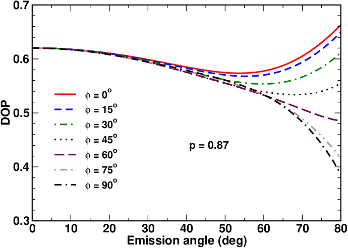
(a) DOP vs emission angle $\theta$ at $p=0.87$

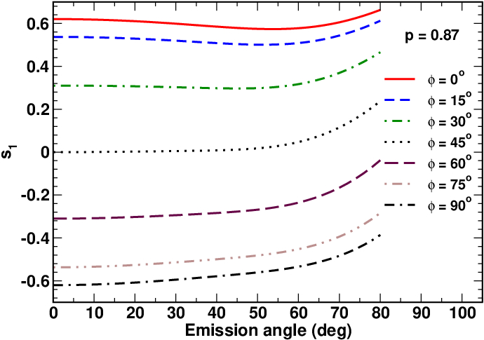
(b) $s_{1}$ vs emission angle $\theta$ at $p=0.87$

Figure 2: Angular profiles of (a) DOP and (b) $s_{1}$ computed at different values of the azimuthal angle $\phi$ for $p=0.87$, $p_{z}=0$ and $u_{\mathrm{em}}=3.85$.

In what follows we concentrate on the four polarization parameters: the degree of linear polarization (DOP) given by Eq. (62), the Stokes parameter $s_{1}$ (see Eq. (63)), the polarization azimuth, $\psi_{p}$, (see Eq. (65)) and the ellipticity $\epsilon_{\mathrm{ell}}$ (see Eq. (66)). Figures 2– 7 present the results for these parameters evaluated as functions of the emission angle $\theta$ at different values of the azimuthal angle $\phi$ (the vector $(-\sin\phi,\cos\phi,0)$ is normal to the emission plane). Calculations are performed for the emission wavelength $\lambda_{\mathrm{em}}=590$ nm assuming that the in-plane extraordinary and ordinary refractive indexes for the azo-dye photoaligning layer of the thickness $D_{a}=15$ nm (the data are taken from Ref. Du et al. (2015)) are $n_{\parallel}^{(a)}=1.8$ and $n_{\perp}^{(a)}=1.5$ (the refractive indices are estimated from the data fitting performed in Ref. Kiselev et al. (2009)), whereas the indexes for the LCP film (for modeling purposes, the thickness is assumed to be $D_{f}=375$ nm) containing NRs with an aspect ratio $5:1$ (the NR length is about $20$ nm and the NR diameter is about $4$ nm) Du et al. (2015) are $n_{\parallel}^{(f)}=1.7$ and $n_{\perp}^{(f)}=1.5$ (typical values for LCs), respectively. Since the LCP molecules are aligned along the easy axis of the SD1 layer, which is perpendicular to the alignment axis of NRs (we assume perfectly in-plane ordering of NRs with $p_{z}=0$ and the alignment axis directed along the $x$ axis) Du et al. (2015), the latter is normal to the in-plane optic axes of both the SD1 layer and the LCP film so that their orientation with respect to the emission plane is defined by the azimuthal angle $\psi$ (see Eq. (18)) which is equal to $\pi/2-\phi$.

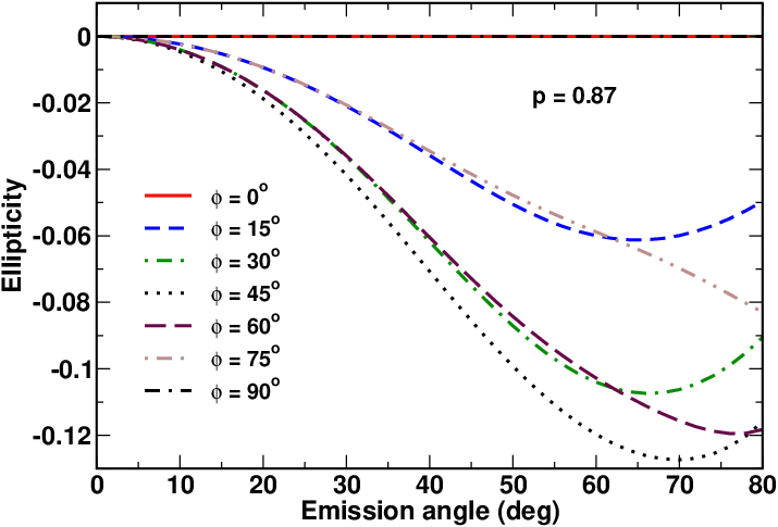
(a) Ellipticity vs emission angle $\theta$ at $p=0.87$

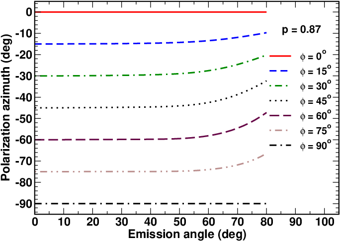
(b) Polarization azimuth vs $\theta$ at $p=0.87$

Figure 3: Angular profiles of (a) ellipticity and (b) polarization azimuth computed at different values of the azimuthal angle $\phi$ for $p=0.87$, $p_{z}=0$ and $u_{\mathrm{em}}=3.85$.

Figures 2 and 3 show the angular profiles computed for highly ordered NRs embedded into the LCP film using the value of the NR alignment order parameter $p=0.87$ reported in Ref. Du et al. (2015). In addition, the value of DOP measured in Du et al. (2015) at $\theta=\phi=0$ is about $0.62$. From this result, we have obtained the estimate for the emission anisotropy parameter: $u_{\mathrm{em}}\approx 3.85$ giving the value of $u_{\mathrm{em}}$ used in our calculations.

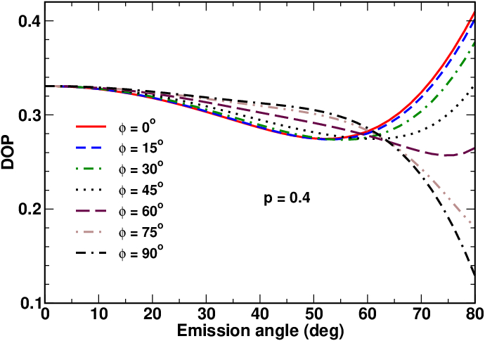
(a) DOP vs emission angle $\theta$ at $p=0.4$

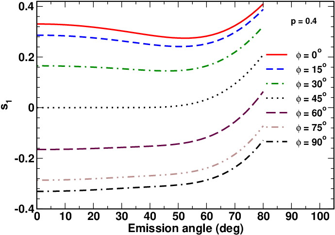
(b) $s_{1}$ vs emission angle $\theta$ at $p=0.4$

Figure 4: Angular profiles of (a) DOP and (b) $s_{1}$ computed at different values of the azimuthal angle $\phi$ for $p=0.4$, $p_{z}=0$ and $u_{\mathrm{em}}=3.85$.

Referring to Fig. 2a, when the azimuthal angle $\phi$ does not exceed $\pi/4$, DOP is generally a nonmonotonic function of the emission angle that increases at sufficiently large values of $\theta$. At $\phi>\pi/4$, DOP monotonically decreases with $\theta$.

In the special case where $\theta=0$ and the detected lightwave is propagating along the normal to the substrates, the value of DOP is independent of $\phi$. As it can be seen from Fig. 3a, at $\theta=0$, the polarized part of the emitted light is linearly polarized and the ellipticity vanishes. In this case, rotation of the emission plane about the $z$ axis by the azimuthal angle $\phi$ is equivalent to the rotation of the sample by the angle $-\phi$. As a result, the polarization plane is rotated by the same angle and, as is indicated in Fig. 3, the polarization azimuth $\psi_{p}$ equals $-\phi$.

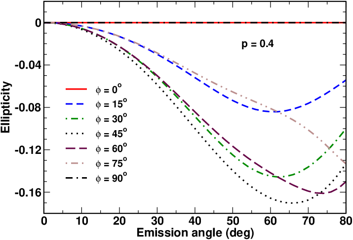
(a) Ellipticity vs emission angle $\theta$ at $p=0.4$

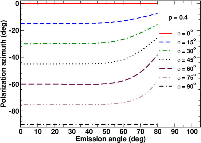
(b) Polarization azimuth vs $\theta$ at $p=0.4$

Figure 5: Angular profiles of (a) ellipticity and (b) polarization azimuth computed at different values of the azimuthal angle $\phi$ for $p=0.4$, $p_{z}=0$ and $u_{\mathrm{em}}=3.85$.

Another consequence of such rotation is that, at $\theta=0$, the Stokes parameter $s_{1}$ changes from $DOP(0)=0.62$ to $-DOP(0)=-0.62$ as $\phi$ varies from zero to $\pi/2$. It immediately follows from the relation

$$s_{1}+is_{2}=DOP\mathrm{e}^{2i\psi_{p}}$$ (71)

that defines the DOP and the polarization azimuth given by Eqs. (62) and (65), respectively. This effect can be seen from the curves presented in Fig. 2b. This figure also demonstrates that, in agreement with the identity (71), $s_{1}(0)$ becomes negative when $\phi>\pi/4$. In this region, $s_{1}$ is a monotonically increasing function of $\theta$, whereas both the magnitude of $s_{1}$, $|s_{1}|$, and the DOP fall as the emission angle increases.

Equation (71) shows that the magnitude of $s_{1}$ is generally smaller than the DOP and the difference between the DOP and $s_{1}$ is dictated by the polarization azimuth $\psi_{p}$. The curves presented in Fig. 3b illustrate a noticeable increase in the polarization azimuth as $\theta$ becomes sufficiently large.

The angular profiles for the ellipticity of the polarized part of the emission plotted in Fig. 3a are computed from Eq. (66). It is found that, for the cases where the alignment axis is either parallel or normal to the emission plane ($\phi=0$ and $\phi=\pi/2$, respectively), the light appears to be linearly polarized and the ellipticity equals zero. At $0<\phi<\pi/2$, this is, however, no longer the case and the ellipticity shows generally nonmonotonic variations with $\theta$. The ellipticity magnitude $|\epsilon_{\mathrm{ell}}|$ reaches its highest value at $\phi=\pi/4$. For $p=0.87$, this value is about $0.12$.

In Figs. 4 and 5, we show what happen when the alignment order parameter is reduced and present the results computed at $p=0.4$. An important point is that the most part of the above discussion being independent of the alignment order parameter remains valid for the case of poorly aligned NRs. So, we will focus our attention on the differences introduced by changes in orientational ordering of NRs.

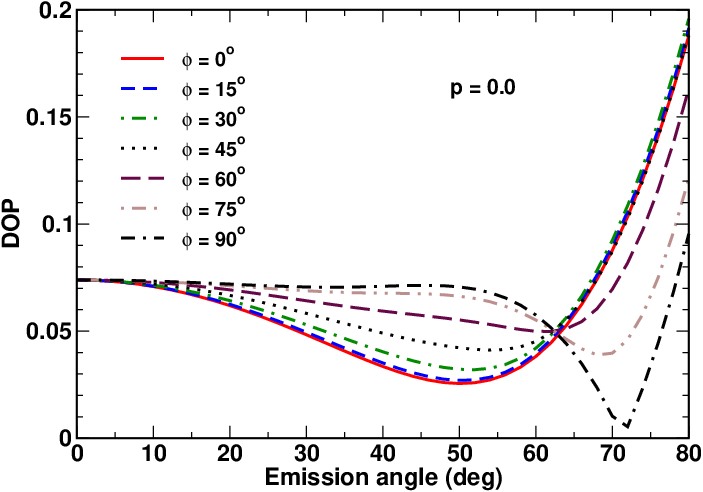
(a) DOP vs emission angle $\theta$ at $p=0$

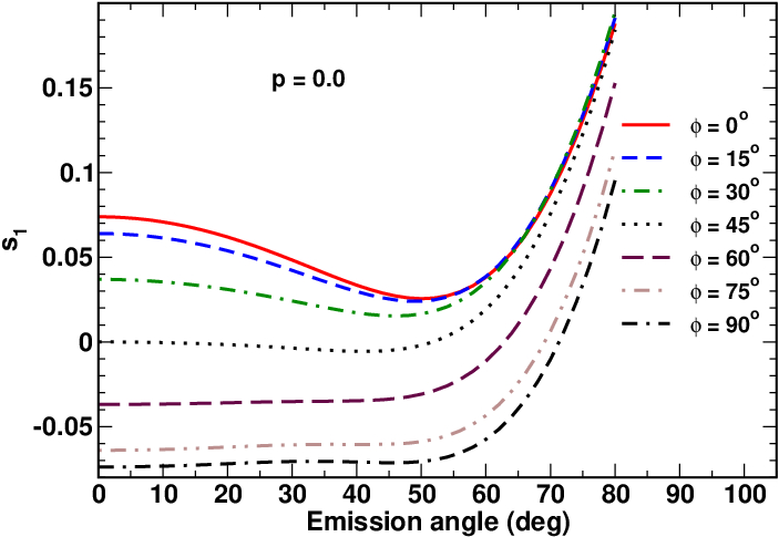
(b) $s_{1}$ vs emission angle $\theta$ at $p=0$

Figure 6: Angular profiles of (a) DOP and (b) $s_{1}$ computed at different values of the azimuthal angle $\phi$ for $p=p_{z}=0$ and $u_{\mathrm{em}}=3.85$.

Referring to Fig. 4a, reduction of the order parameter has a detrimental effect on the DOP. In particular, the value of $DOP(0)$ is reduced to $0.33$. As is seen from Fig. 5a, this effect also manifests itself in an increase of the largest value of the ellipticity magnitude which is now about $0.17$. Qualitatively, the common feature shared by all the angular profiles calculated at $p=0.4$ is that degree of variations and nonmonotic behavior become more pronounced as compared to the case with $p=0.87$.

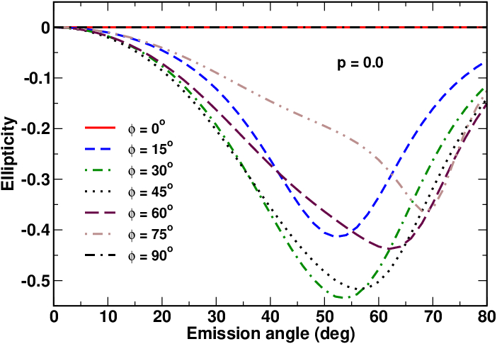
(a) Ellipticity vs emission angle $\theta$ at $p=0$

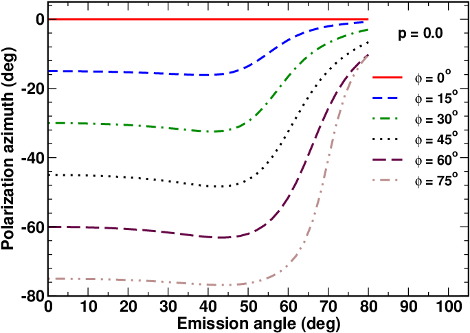
(b) Polarization azimuth vs $\theta$ at $p=0$

Figure 7: Angular profiles of (a) ellipticity and (b) polarization azimuth computed at different values of the azimuthal angle $\phi$ for $p=p_{z}=0$ and $u_{\mathrm{em}}=3.85$.

Figures 6 and 7 demonstrate that this feature is further enhanced in the limiting case of completely disordered NRs with $p=0$. As is shown in Fig. 6, at $p=0$ the values of both the DOP and $|s_{1}|$ experience significant reduction. For instance, $DOP(0)$ is about $0.07$. By contrast, the largest value of the ellipticity magnitude (see Fig. 7a) is increased up to $0.51$. Angular profiles for the polarization azimuth plotted in Fig. 7b demonstrate strong variations and rapidly approach the vicinity of zero as the emission angle increases. Clearly, these features can be regarded as the effects of optically anisotropic environment.

Our concluding remark in this section concerns the parity symmetry of the polarization parameters under the change of sign of the emission and azimuthal angles: $\theta\to-\theta$ and $\phi\to-\phi$. All the polarization parameters are even functions of $\theta$: $DOP(-\theta,\phi)=DOP(\theta,\phi)$, $s_{1}(-\theta,\phi)=s_{1}(\theta,\phi)$, $\epsilon_{\mathrm{ell}}(-\theta,\phi)=\epsilon_{\mathrm{ell}}(\theta,\phi)$ and $\psi_{p}(-\theta,\phi)=\psi(\theta,\phi)$. Similarly, when $\phi$ changes its sign, $DOP$ and $s_{1}$ remain intact: $DOP(\theta,-\phi)=DOP(\theta,\phi)$ and $s_{1}(\theta,-\phi)=s_{1}(\theta,\phi)$. In contrast, the ellipticity and the polarization azimuth are even functions of $\phi$: $\epsilon_{\mathrm{ell}}(\theta,-\phi)=-\epsilon_{\mathrm{ell}}(\theta,\phi)$ and $\psi_{p}(\theta,-\phi)=-\psi_{p}(\theta,\phi)$.

IV Discussion and conclusions

In this paper, we have studied the far-field angular distributions of the polarization parameters characterizing the anisotropy of photoluminescence from orientationally ordered NRs placed inside an optically anisotropic multilayer system. By using a suitably modified version of the transfer matrix method combined with the Green’s function technique we have found the solution of the emission problem expressed in terms of the evolution operators (see Eqs. (44)– (48)). The emission and excitation anisotropy tensors (see Eq. (2) and Eq. (5), respectively) that depend on the transition dipole moments, the exciton level populations and the local field screening factors are then used to deduce the expression for the orientationally averaged coherency matrix (50) of the emitted optical field.

The results of our theoretical analysis are applied to the geometry of the photoalignment method where aligned NRs are embedded into the LCP film placed on top of the photoaligning azo-dye layer Du et al. (2015). By assuming perfectly in-plane ordering of nanorods and unpolarized excitation, we have computed the degree of linear polarization (DOP) (see Eq. (62)), the Stokes parameter $s_{1}$ (see Eq. (63)), the polarization azimuth (see Eq. (65)) and the ellipticity (see Eq. (66)) of the emitted light as functions of the emission and azimuthal angles, $\theta$ and $\phi$, (see Eq. (60)) at different values of the alignment order parameter $p$ (see Eq. (57)). We have found that the values of DOP and the order parameter measured in Ref. Du et al. (2015) can be used to obtain the estimate for the emission anisotropy parameter $u_{\mathrm{em}}$: $u_{\mathrm{em}}\approx 3.75$.

Angular profiles computed as $\theta$ dependencies of the polarization parameters in differently oriented emission planes at varying value of $p$ are presented in Figs. 2– 7. These profiles are shown to be determined by the two coefficients given by Eq. (68) that depend on the NR orientational averages and the emission/excitation anisotropy parameters, while the components of the three matrices given by Eq. (56b) define the angular dependent contributions governed by the optical anisotropy of the LCP film and the photoaligning layer.

We have evaluated the profiles for the three cases: (a) the film with highly ordered NRs ($p=0.87$); (b) the film with poorly ordered NRs ($p=0.4$); and (c) the film with disordered NRs ($p=0.0$). It is found that reduction of orientational order has a detrimental effect on the DOP and the Stokes parameter $s_{1}$ so that their values for the disordered NRs are an order of magnitude smaller than for the highly ordered NRs. By contrast, the largest value of ellipticity significantly grows as the alignment order parameter decreases. The curves computed at $p=0$ (see Figs. 6 and 7) demonstrate a pronounced nonmonotonic behavior that can be regarded as the effect of the optically anisotropic environment.

It should be stressed that the emission and absorption properties of NRs embedded in surrounding dielectric media are generally influenced by the effects of dielectric confinement Rodina and Efros (2016). In our phenomenological approach, NRs are treated as radiating dipoles and these properties are described by the emission and excitation anisotropy tensors. The dielectric confinement effects for dot-in-rods placed in optically anisotropic media has not been studied in any detail yet and analysis of such effects is well beyond the scope of this paper.

We conclude this paper with the remark on the local field effect in the anisotropic LCP film. As it was discussed in Sec. II this effect will typically enhance the anisotropy of emission and excitation leading to nonzero anisotropy parameters $u_{\mathrm{em}}$ and $u_{\mathrm{exc}}$ even if the transition anisotropy is vanishing. For NRs with an aspect ratio $5:1$ and $\epsilon_{\mathrm{em}}\equiv\epsilon_{CdS}=5.23$ Ninomiya and Adachi (1995) embedded in the LCP film with $\epsilon_{\parallel}^{(f)}=2.62$ and $n_{\perp}^{(f)}=2.16$, the screening factors can be estimated assuming that the $c$-axis ($\hat{\mathbf{c}}=\hat{\mathbf{x}}$) is normal to the optic axis of the film directed along the $y$-axis. To this end we can use the well-known analytical results for an optically isotropic ellipsoid placed in the anisotropic medium Sihlova (2008) and evaluate the components, $L_{x}$, $L_{y}$ and $L_{z}$ of the screening factor tensor (dyadic). In our case, this tensor is biaxial. Its diagonal elements are: $L_{z}\approx 0.61<L_{y}\approx 0.67<L_{x}\approx 0.93$ giving the anisotropy ratios: $(L_{x}/L_{z})^{2}\approx 2.33$, $(L_{x}/L_{y})^{2}\approx 1.94$ and $(L_{z}/L_{y})^{2}\approx 0.83$.

These results show that the anisotropic environment plays the role of a symmetry breaking factor and, as a consequence, the transition anisotropy tensor (2) is no longer uniaxial. For instance, in the case of in-plane alignment with $p_{z}=0$, the generalized form of this tensor is as follows

$$\mathbf{J}_{\mathrm{em}}=J_{\mathrm{em}}(\mathbf{I}+u_{\mathrm{em}}\hat{\mathbf{c}}\otimes\hat{\mathbf{c}}+u_{z}\hat{\mathbf{z}}\otimes\hat{\mathbf{z}}),$$ (72)

where $\mathbf{I}$ is the identity matrix. The effect of the local field giving the small negative value of $u_{z}=(L_{z}/L_{y})^{2}-1$ might be further enhanced by the transition anisotropy factor. This may have a profound effect on the angular profiles of the polarization parameters of radiated field. Since the effects of the anisotropic dielectric confinement on the optical properties of nanostructures have not been the subject of intense studies, the physics behind such a phenomenological approach is poorly understood and requires a more sophisticated theoretical treatment.

Appendix A Equations for lateral components

In this section we discuss how to exclude the $z$-components of the electromagnetic field, $E_{z}$ and $H_{z}$, that enter the representation (8), from the Maxwell equations (9). Our task is to derive the closed system of equations for the lateral (tangential) components, $\mathbf{E}_{P}$ and $\mathbf{H}_{P}$.

After substituting Eq. (8) into the Maxwell equations (9), we use decomposition for the differential operator that enter Eq. (9)

$$k_{\mathrm{vac}}^{-1}\boldsymbol{\nabla}=\hat{\mathbf{z}}\,\partial_{\tau}+i\boldsymbol{\nabla}_{P},\quad\boldsymbol{\nabla}_{P}^{\perp}=\hat{\mathbf{z}}\times\boldsymbol{\nabla}_{P},$$ (73)

where $\tau=k_{\mathrm{vac}}z$; $\boldsymbol{\nabla}_{P}=-i\,k_{\mathrm{vac}}^{-1}\,(\hat{\mathbf{x}}\,\partial_{x}+\hat{\mathbf{y}}\,\partial_{y})\equiv(\nabla_{x},\nabla_{y})$ and $\boldsymbol{\nabla}_{P}^{\perp}=(\nabla_{x}^{\perp},\nabla_{y}^{\perp})=(-\nabla_{y},\nabla_{x}),$ to recast Maxwell’s equations (9) into the following form:

$$-i\partial_{\tau}\,[\hat{\mathbf{z}}\times\mathbf{E}_{P}]=\mu\mathbf{H}-\boldsymbol{\nabla}_{P}\times\mathbf{E},$$ (74a)

$$-i\partial_{\tau}\,\mathbf{H}_{P}=\mathbf{D}+\boldsymbol{\nabla}_{P}\times\mathbf{H}+{\mathbf{J}},\quad{\mathbf{J}}\equiv\frac{4\pi i}{ck_{\mathrm{vac}}}\mathbf{J}_{D},$$ (74b)

where the explicit expressions for the last terms on the right hand side of the system (74) are as follows

$$\boldsymbol{\nabla}_{P}\times\mathbf{E}=-\boldsymbol{\nabla}_{P}^{\perp}E_{z}+\bigl{(}{\boldsymbol{\nabla}_{P}^{\perp}}\cdot{\mathbf{E}_{P}}\bigr{)}\,\hat{\mathbf{z}},$$ (75a)

$$\boldsymbol{\nabla}_{P}\times\mathbf{H}=-\boldsymbol{\nabla}_{P}^{\perp}H_{z}+\bigl{(}{\boldsymbol{\nabla}_{P}}\cdot{\mathbf{H}_{P}}\bigr{)}\,\hat{\mathbf{z}}.$$ (75b)

We can now substitute the electric displacement field and the current density of the dipole $\mathbf{J}=-4\pi i\boldsymbol{\mu}_{D}\delta(\mathbf{r}-\mathbf{r}_{0})$ written as a sum of the normal and in-plane components

$$\mathbf{D}=D_{z}\hat{\mathbf{z}}+\mathbf{D}_{P},\quad\mathbf{J}=J_{z}\hat{\mathbf{z}}+\mathbf{J}_{P},$$ (76)

into Eq. (74b) and derive the following expression for its $z$-component

$$D_{z}=\epsilon_{zz}E_{z}+\bigl{(}{\boldsymbol{\epsilon}_{z}}\cdot{\mathbf{E}_{P}}\bigr{)}=-\bigl{(}{\boldsymbol{\nabla}_{P}}\cdot{\mathbf{H}_{P}}\bigr{)}-{J}_{z},$$ (77)

where $\boldsymbol{\epsilon}_{z}=(\epsilon_{zx},\epsilon_{zy})$.

From Eqs. (74) and (77), it is not difficult to deduce the relations

$$H_{z}=\mu^{-1}\bigl{(}{\boldsymbol{\nabla}_{P}^{\perp}}\cdot{\mathbf{E}_{P}}\bigr{)}$$ (78)

$$E_{z}=-\epsilon_{zz}^{-1}\bigl{[}\bigl{(}{\boldsymbol{\epsilon}_{z}}\cdot{\mathbf{E}_{P}}\bigr{)}+\bigl{(}{\boldsymbol{\nabla}_{P}}\cdot{\mathbf{H}_{P}}\bigr{)}+{J}_{z}\bigr{]}$$ (79)

linking the normal (along the $z$ axis) and the lateral (perpendicular to the $z$ axis) components.

By using the relation (79), we obtain the tangential component of the field (76)

$$\mathbf{D}_{P}=\boldsymbol{\epsilon}_{z}^{\,\prime}E_{z}+\boldsymbol{\varepsilon}_{z}\cdot\mathbf{E}_{P}=\boldsymbol{\varepsilon}_{P}\cdot\mathbf{E}_{P}-\boldsymbol{\epsilon}_{z}^{\,\prime}\,\epsilon_{zz}^{-1}\bigl{[}\bigl{(}{\boldsymbol{\nabla}_{P}}\cdot{\mathbf{H}_{P}}\bigr{)}+{J}_{z}\bigr{]}$$ (80)

where $\boldsymbol{\varepsilon}_{z}=\begin{pmatrix}\epsilon_{xx}&\epsilon_{xy}\\ \epsilon_{yx}&\epsilon_{yy}\end{pmatrix}$; $\boldsymbol{\epsilon}_{z}^{\,\prime}=(\epsilon_{xz},\epsilon_{yz})$ and the effective dielectric tensor, $\boldsymbol{\varepsilon}_{P}$, for the lateral components is given by

$$\boldsymbol{\varepsilon}_{P}=\boldsymbol{\varepsilon}_{z}-\epsilon_{zz}^{-1}\,\boldsymbol{\epsilon}_{z}^{\,\prime}\otimes\boldsymbol{\epsilon}_{z}.$$ (81)

Maxwell’s equations (74) can now be combined with the relations (75) to yield the system

$$-i\partial_{\tau}\,\mathbf{E}_{P}=\mu\mathbf{H}_{P}+\boldsymbol{\nabla}_{P}E_{z},$$ (82a)

$$-i\partial_{\tau}\,\mathbf{H}_{P}=\mathbf{D}_{P}-\boldsymbol{\nabla}_{P}^{\perp}H_{z}+{\mathbf{J}}_{P},$$ (82b)

where $H_{z}$, $E_{z}$ and $\mathbf{D}_{P}$ are given in Eq. (78), Eq. (79) and Eq. (80), respectively.

So, this system immediately gives the final result

$$-i\partial_{\tau}\,\mathbf{E}_{P}=-\boldsymbol{\nabla}_{P}[\epsilon_{zz}^{-1}\bigl{(}{\boldsymbol{\epsilon}_{z}}\cdot{\mathbf{E}_{P}}\bigr{)}]+\mu\mathbf{H}_{P}-\boldsymbol{\nabla}_{P}\epsilon_{zz}^{-1}[\bigl{(}{\boldsymbol{\nabla}_{P}}\cdot{\mathbf{H}_{P}}\bigr{)}+{J}_{z}],$$ (83a)

$$-i\partial_{\tau}\,\mathbf{H}_{P}=\boldsymbol{\varepsilon}_{P}\cdot\mathbf{E}_{P}-\boldsymbol{\nabla}_{P}^{\perp}[\bigl{(}{\boldsymbol{\nabla}_{P}^{\perp}}\cdot{\mathbf{E}_{P}}\bigr{)}/\mu]-\boldsymbol{\epsilon}_{z}^{\,\prime}\,\epsilon_{zz}^{-1}[\bigl{(}{\boldsymbol{\nabla}_{P}}\cdot{\mathbf{H}_{P}}\bigr{)}+{J}_{z}]+{\mathbf{J}}_{P},$$ (83b)

that can be easily rewritten in the matrix form used in Sec. II.

References

- Hu et al. (2001) J. Hu, L.-s. Li, W. Yang, L. Manna, L.-w. Wang, and A. P. Alivisatos, Science 292, 2060 (2001).
- Shabaev and Efros (2004) A. Shabaev and A. L. Efros, Nano Letters 4, 1821 (2004).
- Talapin et al. (2003) D. V. Talapin, R. Koeppe, S. Götzinger, A. Kornowski, J. M. Lupton, A. L. Rogach, O. Benson, J. Feldmann, and H. Weller, Nano Letters 3, 1677 (2003).
- Sitt et al. (2011) A. Sitt, A. Salant, G. Menagen, and U. Banin, Nano Letters 11, 2054 (2011).
- Rainó et al. (2012) G. Rainó, T. Stöferle, I. Moreels, R. Gomes, Z. Hens, and R. F. Mahrt, ACS Nano 6, 1979 (2012).
- Vezzoli et al. (2015) S. Vezzoli, M. Manceau, G. Leménager, Q. Glorieux, E. Giacobino, L. Carbone, M. De Vittorio, and A. Bramati, ACS Nano 9, 7992 (2015).
- Hasegawa et al. (2015) M. Hasegawa, Y. Hirayama, and S. Dertinger, Applied Physics Letters 106, 051103 (2015).
- Aubert et al. (2015) T. Aubert, L. Palangetic, M. Mohammadimasoudi, K. Neyts, J. Beeckman, C. Clasen, and Z. Hens, ACS Photonics 2, 583 (2015).
- Krahne et al. (2011) R. Krahne, G. Morello, A. Figuerola, C. George, S. Deka, and L. Manna, Physics Reports 501, 75 (2011), ISSN 0370-1573.
- Hens and Moreels (2012) Z. Hens and I. Moreels, J. Mater. Chem. 22, 10406 (2012).
- Kamal et al. (2012) J. S. Kamal, R. Gomes, Z. Hens, M. Karvar, K. Neyts, S. Compernolle, and F. Vanhaecke, Phys. Rev. B 85, 035126 (2012).
- Angeloni et al. (2016) I. Angeloni, W. Raja, R. Brescia, A. Polovitsyn, F. De Donato, M. Canepa, G. Bertoni, R. Proietti Zaccaria, and I. Moreels, ACS Photonics 3, 58 (2016).
- Efros (1992) A. L. Efros, Phys. Rev. B 46, 7448 (1992).
- Chen et al. (2001) X. Chen, A. Nazzal, D. Goorskey, M. Xiao, Z. A. Peng, and X. Peng, Phys. Rev. B 64, 245304 (2001).
- Kazes et al. (2002) M. Kazes, D. Lewis, Y. Ebenstein, T. Mokari, and U. Banin, Advanced Materials 14, 317 (2002).
- Yong et al. (2009) K.-T. Yong, R. Hu, I. Roy, H. Ding, L. A. Vathy, E. J. Bergey, M. Mizuma, A. Maitra, and P. N. Prasad, ACS Applied Materials & Interfaces 1, 710 (2009).
- Pisanello et al. (2010) F. Pisanello, L. Martiradonna, P. Spinicelli, A. Fiore, J. Hermier, L. Manna, R. Cingolani, E. Giacobino, M. D. Vittorio, and A. Bramati, Superlattices and Microstructures 47, 165 (2010), ISSN 0749-6036.
- Cunningham et al. (2016) P. D. Cunningham, J. a. B. Souza, I. Fedin, C. She, B. Lee, and D. V. Talapin, ACS Nano 10, 5769 (2016).
- Srivastava et al. (2017) A. K. Srivastava, W. Zhang, J. Schneider, A. L. Rogach, V. G. Chigrinov, and H.-S. Kwok, Advanced Materials 29, 1701091 (2017).
- Mohammadimasoudi et al. (2013) M. Mohammadimasoudi, L. Penninck, T. Aubert, R. Gomes, Z. Hens, F. Strubbe, and K. Neyts, Opt. Mater. Express 3, 2045 (2013).
- Du et al. (2015) T. Du, J. Schneider, A. K. Srivastava, A. S. Susha, V. G. Chigrinov, H. S. Kwok, and A. L. Rogach, ACS Nano 9, 11049 (2015).
- Schneider et al. (2017) J. Schneider, W. Zhang, A. K. Srivastava, V. G. Chigrinov, H.-S. Kwok, and A. L. Rogach, Nano Letters 17, 3133 (2017).
- Fourkas (2001) J. T. Fourkas, Opt. Lett. 26, 211 (2001).
- Böhmer and Enderlein (2003) M. Böhmer and J. Enderlein, J. Opt. Soc. Am. B 20, 554 (2003).
- Lieb et al. (2004) M. A. Lieb, J. M. Zavislan, and L. Novotny, J. Opt. Soc. Am. B 21, 1210 (2004).
- Empedocles et al. (1999) S. A. Empedocles, R. Neuhauser, and M. G. Bawendi, Nature 399, 126 (1999).
- Lethiec et al. (2014a) C. Lethiec, J. Laverdant, H. Vallon, C. Javaux, B. Dubertret, J.-M. Frigerio, C. Schwob, L. Coolen, and A. Maître, Phys. Rev. X 4, 021037 (2014a).
- Lukosz and Kunz (1977a) W. Lukosz and R. E. Kunz, J. Opt. Soc. Am. 67, 1607 (1977a).
- Lukosz and Kunz (1977b) W. Lukosz and R. E. Kunz, J. Opt. Soc. Am. 67, 1615 (1977b).
- Lukosz (1979) W. Lukosz, J. Opt. Soc. Am. 69, 1495 (1979).
- Lukosz (1981) W. Lukosz, J. Opt. Soc. Am. 71, 744 (1981).
- Lethiec et al. (2014b) C. Lethiec, F. Pisanello, L. Carbone, A. Bramati, L. Coolen, and A. Ma ̂itre, New Journal of Physics 16, 093014 (2014b).
- Wackenhut et al. (2012) F. Wackenhut, A. Virgilio Failla, T. Züchner, M. Steiner, and A. J. Meixner, Applied Physics Letters 100, 263102 (2012).
- Kim et al. (2017) J. Kim, S. Michelin, M. Hilbers, L. Martinelli, E. Chaudan, G. Amselem, E. Fradet, J.-P. Boilot, A. M. Brouwer, C. N. Baroud, et al., Nature Nanotechnology 12, 914 (2017).
- Flämmich et al. (2010) M. Flämmich, M. Gather, N. Danz, D. Michaelis, A. Bräuer, K. Meerholz, and A. Tünnermann, Organic Electronics 11, 1039 (2010).
- Shakya et al. (2005) J. Shakya, K. Knabe, K. H. Kim, J. Li, J. Y. Lin, and H. X. Jiang, Applied Physics Letters 86, 091107 (2005).
- Schubert et al. (2007) M. F. Schubert, S. Chhajed, J. K. Kim, E. Fred Schubert, and J. Cho, Applied Physics Letters 91, 051117 (2007).
- Krames et al. (2007) M. R. Krames, O. B. Shchekin, R. Mueller-Mach, G. O. Mueller, L. Zhou, G. Harbers, and M. G. Craford, J. Display Technol. 3, 160 (2007).
- Matioli and Weisbuch (2011) E. Matioli and C. Weisbuch, Journal of Applied Physics 109, 073114 (2011).
- Yuan et al. (2014) G. Yuan, X. Chen, T. Yu, H. Lu, Z. Chen, X. Kang, J. Wu, and G. Zhang, Journal of Applied Physics 115, 093106 (2014).
- Gu et al. (2014) L. Gu, J. E. Livenere, G. Zhu, T. U. Tumkur, H. Hu, C. L. Cortes, Z. Jacob, S. M. Prokes, and M. A. Noginov, Scientific Reports 4, 7327 (2014).
- Efros et al. (1996) A. L. Efros, M. Rosen, M. Kuno, M. Nirmal, D. J. Norris, and M. Bawendi, Phys. Rev. B 54, 4843 (1996).
- Rodina and Efros (2016) A. V. Rodina and A. L. Efros, Journal of Experimental and Theoretical Physics 122, 554 (2016), ISSN 1090-6509.
- Choy (2016) T. C. Choy, Effective Medium Theory: Principles and Applications, vol. 165 of International Series Of Monographs On Physics (Oxford University Press, Oxford, 2016), 2nd ed.
- Sihlova (2008) A. Sihlova, Electromagnetic Mixing Formulas and Applications, vol. 47 of IET Electromagnetic Waves Series (The Institution of Engineering and Technology, London, 2008).
- Gordon and Gartstein (2014) J. M. Gordon and Y. N. Gartstein, J. Opt. Soc. Am. B 31, 2029 (2014).
- Battie et al. (2014) Y. Battie, A. En Naciri, W. Chamorro, and D. Horwat, The Journal of Physical Chemistry C 118, 4899 (2014).
- Zhang et al. (2018) W. Zhang, J. Schneider, V. G. Chigrinov, H. S. Kwok, A. L. Rogach, and A. K. Srivastava, Advanced Optical Materials 6, 1800250 (2018).
- Reshetnyak et al. (2018) V. Y. Reshetnyak, I. P. Pinkevych, T. J. Sluckin, A. M. Urbas, and D. R. Evans, The European Physical Journal Plus 133, 373 (2018).
- Kiselev et al. (2004) A. D. Kiselev, O. V. Yaroshchuk, and L. Dolgov, J. Phys.: Condens. Matter 16, 7183 (2004).
- Shelestiuk et al. (2011) S. M. Shelestiuk, V. Y. Reshetnyak, and T. J. Sluckin, Phys. Rev. E 83, 041705 (2011).
- Fuh et al. (2013) A. Y.-G. Fuh, W. Lee, and K. Y.-C. Huang, Liquid Crystals 40, 745 (2013).
- Kidwai et al. (2012) O. Kidwai, S. V. Zhukovsky, and J. E. Sipe, Phys. Rev. A 85, 053842 (2012).
- Zhang and Wu (2015) X. Zhang and Y. Wu, Scientific Reports 5, 7892 (2015).
- Li and Khurgin (2016) T. Li and J. B. Khurgin, Optica 3, 1388 (2016).
- Zhang and Zhang (2017) R. Z. Zhang and Z. M. Zhang, Journal of Quantitative Spectroscopy and Radiative Transfer 197, 132 (2017), ISSN 0022-4073.
- Lei et al. (2017) X. Lei, L. Mao, Y. Lu, and P. Wang, Phys. Rev. B 96, 035439 (2017).
- Markoš and Soukoulis (2008) P. Markoš and C. M. Soukoulis, Wave Propagation: From Electrons to Photonic Crystals and Left-Handed Materials (Princeton Univ. Press, Princeton and Oxford, 2008).
- Yariv and Yeh (2007) A. Yariv and P. Yeh, Photonics: Optical Electronics in Modern Communications (Oxford University Press, New York, 2007), 6th ed.
- Kiselev (2007) A. D. Kiselev, J. Phys.: Condens. Matter 19, 246102 (2007).
- Kiselev et al. (2008) A. D. Kiselev, R. G. Vovk, R. I. Egorov, and V. G. Chigrinov, Phys. Rev. A 78, 033815 (2008).
- Kiselev and Vovk (2010) A. D. Kiselev and R. G. Vovk, JETP 110, 901 (2010).
- Kiselev et al. (2011) A. D. Kiselev, E. P. Pozhidaev, V. G. Chigrinov, and H.-S. Kwok, Phys. Rev. E 83, 031703 (2011).
- Kiselev and Chigrinov (2014) A. D. Kiselev and V. G. Chigrinov, Phys. Rev. E 90, 042504 (2014).
- Novotny and Hecht (2006) L. Novotny and B. Hecht, Principles of Nano-Optics (Cambridge Univ. Press, New York, 2006).
- Mandel and Wolf (1995) L. Mandel and E. Wolf, Optical Coherence and Quantum Optics (Cambridge University Press, Cambridge, 1995).
- Clemmow (1996) P. C. Clemmow, The Plane Wave Spectrum Representation of Electromagnetic Fields, IEEE/OUP Series on Electromagnetic Wave Theory (Oxford University Press, Oxford, 1996).
- Born and Wolf (1999) M. Born and E. Wolf, Principles of Optics: Electromagnetic Theory of Propagation, Interference and Diffraction of Light (Cambridge Univ. Press, New York, 1999), 7th ed.
- Kiselev et al. (2009) A. D. Kiselev, V. G. Chigrinov, and H.-S. Kwok, Phys. Rev. E 80, 011706 (2009).
- Ninomiya and Adachi (1995) S. Ninomiya and S. Adachi, Journal of Applied Physics 78, 1183 (1995).