The Bottom-up Evolution of Representations in the Transformer:
A Study with Machine Translation and Language Modeling Objectives

Abstract

We seek to understand how the representations of individual tokens and the structure of the learned feature space evolve between layers in deep neural networks under different learning objectives. We focus on the Transformers for our analysis as they have been shown effective on various tasks, including machine translation (MT), standard left-to-right language models (LM) and masked language modeling (MLM). Previous work used black-box probing tasks to show that the representations learned by the Transformer differ significantly depending on the objective. In this work, we use canonical correlation analysis and mutual information estimators to study how information flows across Transformer layers and how this process depends on the choice of learning objective. For example, as you go from bottom to top layers, information about the past in left-to-right language models gets vanished and predictions about the future get formed. In contrast, for MLM, representations initially acquire information about the context around the token, partially forgetting the token identity and producing a more generalized token representation. The token identity then gets recreated at the top MLM layers.

1 Introduction

Deep (i.e. multi-layered) neural networks have become the standard approach for many natural language processing (NLP) tasks, and their analysis has been an active topic of research. One popular approach for analyzing representations of neural models is to evaluate how informative they are for various linguistic tasks, so-called “probing tasks”. Previous work has made some interesting observations regarding these representations; for example, Zhang and Bowman (2018) show that untrained LSTMs outperform trained ones on a word identity prediction task; and Blevins et al. (2018) show that up to a certain layer performance of representations obtained from a deep LM improves on a constituent labeling task, but then decreases, while with representations obtained from an MT encoder performance continues to improve up to the highest layer. These observations have, however, been somewhat anecdotal and an explanation of the process behind such behavior has been lacking.

In this paper, we attempt to explain more generally why such behavior is observed. Rather than measuring the quality of representations obtained from a particular model on some auxiliary task, we characterize how the learning objective determines the information flow in the model. In particular, we consider how the representations of individual tokens in the Transformer evolve between layers under different learning objectives.

We look at this task from the information bottleneck perspective on learning in neural networks. Tishby and Zaslavsky (2015) state that “the goal of any supervised learning is to capture and efficiently represent the relevant information in the input variable about the output-label variable” and hence the representations undergo transformations which aim to encode as much information about the output label as possible, while ‘forgetting’ irrelevant details about the input. As we study sequence encoders and look into representations of individual tokens rather than the entire input, our situation is more complex. In our model, the information preserved in a representation of a token is induced due to two roles it plays: (i) predicting the output label from a current token representation; (ii) preserving information necessary to build representations of other tokens. For example, a language model constructs a representation which is not only useful for predicting an output label (in this case, the next token), but also informative for producing representations of subsequent tokens in a sentence. This is different from the MT setting, where there is no single encoder state from which an output label is predicted. We hypothesize that the training procedure (or, in our notation, the task) defines

1. the nature of changes a token representation undergoes, from layer to layer;

2. the process of interactions and relationships between tokens;

3. the type of information which gets lost and acquired by a token representation in these interactions.

In this work, we study how the choice of objective affects the process by which information is encoded in token representations of the Transformer Vaswani et al. (2017), as this architecture achieves state-of-the-art results on tasks with very different objectives such as machine translation (MT) Bojar et al. (2018); Niehues et al. (2018), standard left-to-right language modeling (LM) Radford et al. (2018) and masked language modeling (MLM) Devlin et al. (2018). The Transformer encodes a sentence by iteratively updating representations associated with each token starting from a context-agnostic representation consisting of a positional and a token embedding. At each layer token representations exchange information among themselves via multi-head attention and then this information is propagated to the next layer via a feed-forward transformation. We investigate how this process depends on the choice of objective function (LM, MLM or MT) while keeping the data and model architecture fixed.

We start with illustrating the process of information loss and gain in representations of individual tokens by estimating the mutual information between token representations at each layer and the input token identity (i.e. the word type) or the output label (e.g., the next word for LM).

Then, we investigate behavior of token representations from two perspectives: how they influence and are influenced by other tokens. Using canonical correlation analysis, we evaluate the extent of change the representation undergoes and the degree of influence. We reveal differences in the patterns of this behavior for different tasks.

Finally, we study which type of information gets lost and gained in the interactions between tokens and to what extent a certain property is important for defining a token representation at each layer and for each task. As the properties, we consider token identities (‘word type’), positions, identities of surrounding tokens and CCG supertags. In these analyses we rely on similarity computations.

We find, that (1) with the LM objective, as you go from bottom to top layers, information about the past gets lost and predictions about the future get formed; (2) for MLMs, representations initially acquire information about the context around the token, partially forgetting the token identity and producing a more generalized token representation; the token identity then gets recreated at the top layer; (3) for MT, though representations get refined with context, less processing is happening and most information about the word type does not get lost. This provides us with a hypothesis for why the MLM objective may be preferable in the pretraining context to LM. LMs may not be the best choice, because neither information about current token and its past nor future is represented well: the former since this information gets discarded, the latter since the model does not have access to the future.

Our key contributions are as follows:

• we propose to view the evolution of a token representation between layers from the compression/prediction trade-off perspective;

• we conduct a series of experiments supporting this view and showing that the two processes, losing information about input and accumulating information about output, take place in the evolution of representations (for MLM, these processes are clearly distinguished and can be viewed as two stages, ‘context encoding’ and ‘token prediction’);

• we relate to some findings from previous work, putting them in the proposed perspective, and provide insights into the internal workings of Transformer trained with different objectives;

• we propose an explanation for superior performance of the MLM objective over the LM one for pretraining.

All analysis is done in a model-agnostic manner by investigating properties of token representations at each layer, and can, in principle, be applied to other multi-layer deep models (e.g., multi-layer RNN encoders).

2 Tasks

In this section, we describe the tasks we consider. For each task, we define input $X$ and output $Y$.

2.1 Machine translation

Given source sentence $X\!=\!(x_{1},x_{2},...,x_{S})$ and a target sentence $Y\!=\!(y_{1},y_{2},...,y_{T})$, NMT models predict words in the target sentence, word by word, i.e. provide estimates of the conditional distribution $p(y_{i}|X,y_{1,i-1},\theta)$.

We train a standard Transformer for the translation task and then analyze its encoder. In contrast to the other two tasks we describe below, representations from the top layers are not directly used to predict output labels but to encode the information which is then used by the decoder.

2.2 Language modeling

LMs estimate the probability of a word given the previous words in a sentence $P(x_{t}|x_{1},\dots,x_{t-1},\theta)$. More formally, the model is trained with inputs $X=(x_{1},\dots,x_{t-1})$ and outputs $Y=(x_{t})$, where $x_{t}$ is the output label predicted from the final (i.e. top-layer) representation of a token $x_{t-1}$. It is straightforward to apply the Transformer to this task (Radford et al., 2018; Lample and Conneau, 2019).

2.3 Masked language modeling

We also consider the MLM objective Devlin et al. (2018), randomly sampling $15\%$ of the tokens to be predicted. We replace the corresponding input token by [MASK] or a random token in $80\%$ and $10\%$ of the time, respectively, keeping it unchanged otherwise.

For a sentence $(x_{1},x_{2},...,x_{S})$, where token $x_{i}$ is replaced with $\tilde{x_{i}}$, the model receives $X\!=\!(x_{1},\dots,x_{i-1},\tilde{x_{i}},x_{i+1},\dots,x_{S})$ as input and needs to predict $Y\!=\!(x_{i})$. The label $x_{i}$ is predicted from the final representation of the token $\tilde{x_{i}}$.

3 Data and Setting

As described below, for a fair comparison, we use the same training data, model architecture and parameter initialization across all the tasks. In order to make sure that our findings are reliable, we also use multiple datasets and repeat experiments with different random initializations for each task.

We train all models on the data from the WMT news translation shared task. We conduct separate series of experiments using two language pairs: WMT 2017 English-German (5.8m sentence pairs) and WMT 2014 English-French (40.8m sentence pairs). For language modeling, we use only the source side of the parallel data. We remove randomly chosen 2.8m sentence pairs from the English-French dataset and use the source side for analysis. English-French models are trained on the remaining 38m sentence pairs. We consider different dataset sizes (2.5m and 5.8m for English-German, 2.5m, 5.8m and 38m for English-French). We find that our findings are true for all languages, dataset sizes and initializations. In the following, all the illustrations are provided for the models trained on the full English-German dataset (5.8m sentence pairs).

We follow the setup and training procedure of the Transformer base model Vaswani et al. (2017). For details, see the appendix.

4 The Information-Bottleneck Viewpoint

In this section, we give an intuitive explanation of the Information Bottleneck (IB) principle Tishby et al. (1999) and consider a direct application of this principle to our analysis.

4.1 Background

The IB method Tishby et al. (1999) considers a joint distribution of input-output pairs $p(X,Y)$ and aims to extract a compressed representation $\tilde{X}$ for an input $X$ such that $\tilde{X}$ retains as much as possible information about the output $Y$. More formally, the IB method maximizes the mutual information (MI) with the output $I(\tilde{X};Y)$, while penalizing for MI with the input $I(\tilde{X};X)$. The latter term in the objective ensures that the representation is indeed a compression. Intuitively, the choice of the output variable $Y$ determines the split of $X$ into irrelevant and relevant features. The relevant features need to be retained while irrelevant ones should be dropped.

Tishby and Zaslavsky (2015) argue that computation in a multi-layered neural model can be regarded as an evolution towards the theoretical optimum of the IB objective. A sequence of layers is viewed as a Markov chain, and the process of obtaining $Y$ corresponds to compressing the representation as it flows across layers and retaining only information relevant to predicting $Y$. This implies that $Y$ defines the information flow in the model. Since $Y$ is different for each model, we expect to see different patterns of information flow in models, and this is the focus of our study.

4.2 IB for token representations

In this work, we view every sequence model (MT, LM and MLM) as learning a function from input $X$ to output $Y$. The input is a sequence of tokens $X=(x_{1},x_{2},\dots,x_{n})$ and the output $Y$ is defined in Section 2. Recall that we focus on representations of individual tokens in every layer rather than the representation of the entire sequence.

We start off our analysis of divergences in the information flow for different objectives by estimating the amount of information about input or output tokens retained in the token representation at each layer.

4.2.1 Estimating mutual information

Inspired by Tishby and Zaslavsky (2015), we estimate MI between token representations at a certain layer and an input token. To estimate MI, we need to consider token representations at a layer as samples from a discrete distribution. To get such distribution, in the original works Shwartz-Ziv and Tishby (2017), the authors binned the neuron’s $\arctan$ activations. Using these discretized values for each neuron in a layer, they were able to treat a layer representation as a discrete variable. They considered neural networks with maximum 12 neurons at a layer, but in practical scenarios (e.g. we have 512 neurons in each layer) this approach is not feasible. Instead, similarly to Sajjadi et al. (2018), we discretize the representations by clustering them into a large number of clusters. Then we use cluster labels instead of the continuous representations in the MI estimator.

Specifically, we take only representations of the 1000 most frequent (sub)words. We gather representations for 5 million occurrences of these at each layer for each of the three models. We then cluster the representations into $N=10000$ clusters using mini-batch $k$-means with $k=100$. In the experiments studying the mutual information between a layer and source (or target) labels we further filter occurrences. Namely, we take only occurrences where the source and target labels are among the top 1000 most frequent (sub)words.

4.2.2 Results

Figure 1: The mutual information between an input token and a representation of this token at each layer.

(a) LM

(b) MLM

Figure 2: The mutual information of token representations at a layer and source (or target) tokens. For MLM, only tokens replaced at random are considered to get examples where input and output are different.

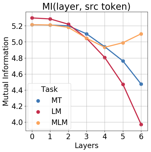
First, we estimate the MI between an input token and a representation of this token at each layer. In this experiment, we form data for MLM as in the test regime; in other words, the input token is always the same as the output token. Results are shown in Figure 1. For LM, the amount of relevant information about the current input token decreases. This agrees with our expectations: some of the information about the history is intuitively not relevant for predicting the future. MT shows a similar behavior, but the decrease is much less sharp. This is again intuitive: the information about the exact identity is likely to be useful for the decoder. The most interesting and surprising graph is for MLM: first, similarly to other models, the information about the input token is getting lost but then, at two top layers, it gets recovered. We will refer to these phases in further discussion as context encoding and token reconstruction, respectively. Whereas such non-monotonic behavior is impossible when analyzing entire layers, as in Tishby and Zaslavsky (2015), in our case, it suggests that this extra information is obtained from other tokens in the context.

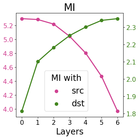
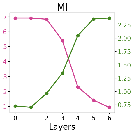
We perform the same analysis but now measuring MI with the output label for LM and MLM. In this experiment, we form data for MLM as in training, masking or replacing a fraction of tokens. We then take only tokens replaced with a random one to get examples where input and output tokens are different. Results are shown in Figure 2. We can see that, as expected, MI with input tokens decreases while MI with output tokens increases. Both LM and MLM are trained to predict a token (next for LM and current for MLM) by encoding input and context information. While in Figure 1 we observed monotonic behavior of LM, when looking at the information with both input and output tokens, we can see the two processes, losing information about input and accumulating information about output, for both LM and MLM models. For MLM these processes are more distinct and can be thought of as the context encoding and token prediction (compression/prediction) stages. For MT, since nothing is predicted directly, we see only the encoding stage of this process. This observation relates also to the findings by Blevins et al. (2018). They show that up to a certain layer the performance of representations obtained from a deep multi-layer RNN LM improves on a constituent labeling task, but then decreases, while for representations obtained from an MT encoder performance continues to improve up to the highest layer. We further support this view with other experiments in Section 6.3.

Even though the information-theoretic view provides insights into processes shaping the representations, direct MI estimation from finite samples for densities on multi-dimensional spaces is challenging Paninski (2003). For this reason in the subsequent analysis we use more well-established frameworks such as canonical correlation analysis to provide new insights and also to corroborate findings we made in this section (e.g., the presence of two phases in MLM encoding). Even though we will be using different machinery, we will focus on the same two IB-inspired questions: (1) how does information flow across layers? and (2) what information does a layer represent?

5 Analyzing Changes and Influences

In this section, we analyze the flow of information. The questions we ask include: how much processing is happening in a given layer; which tokens influence other tokens most; which tokens gain most information from other tokens. As we will see, these questions can be reduced to a comparison between network representations. We start by describing the tool we use.

5.1 Canonical Correlation Analysis

We rely on recently introduced projection weighted Canonical Correlation Analysis (PWCCA) Morcos et al. (2018), which is an improved version of SVCCA Raghu et al. (2017). Both approaches are based on classic Canonical Correlation Analysis (CCA) Hotelling (1936).

CCA is a multivariate statistical method for relating two sets of observations arising from an underlying process. In our setting, the underlying process is a neural network trained on some task. The two sets of observations can be seen as ‘two views’ on the data. Intuitively, we look at the same data (tokens in a sentence) from two standpoints. For example, one view is one layer and another view is another layer. Alternatively, one view can be $l$-th layer in one model, whereas another view can be the same $l$-th layer in another model. CCA lets us measure similarity between pairs of views.

Formally, given a set of tokens $(x_{1},x_{2},\dots,x_{N})$ (with the sentences they occur in), we gather their representations produced by two models ($m_{1}$ and $m_{2}$) at layers $l_{1}$ and $l_{2}$, respectively. To achieve this, we encode the whole sentences and take representations of tokens we are interested in. We get two views of these tokens by the models: $v^{m_{1},l_{1}}\!=\!(x_{1}^{m_{1},l_{1}},x_{2}^{m_{1},l_{1}},\dots,x_{N}^{m_{1},l_{1}})$ and $v^{m_{2},l_{2}}\!=\!(x_{1}^{m_{2},l_{2}},x_{2}^{m_{2},l_{2}},\dots,x_{N}^{m_{2},l_{2}})$. The representations are gathered in two matrices $X_{1}\!\in\!M_{a,N}$ and $X_{2}\!\in\!M_{b,N}$, where $a$ and $b$ are the numbers of neurons in the models. These matrices are then given to CCA (specifically, PWCCA). CCA identifies a linear relation maximizing the correlation between the matrices and computes the similarity. The values of PWCCA range from 0 to 1, with 1 indicating that the observations are linear transformations of each other, 0 indicating no correlation.

In the next sections, we vary two aspects of this process: tokens and the ‘points of view’.

5.2 A coarse-grained view

We start with the analysis where we do not attempt to distinguish between different token types.

5.2.1 Distances between tasks

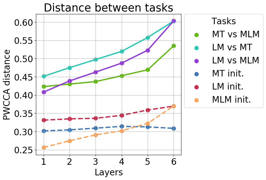
As the first step in our analysis, we measure the difference between representations learned for different tasks. In other words, we compare representations for $v^{m_{1},l}$ and $v^{m_{2},l}$ at different layers $l$. Here the data is all tokens of 5000 sentences. We also quantify differences between representations of models trained with the same objective but different random initializations. The results are provided in Figure 3(a).

First, differences due to training objective are much larger than the ones due to random initialization of a model. This indicates that PWCCA captures underlying differences in the types of information learned by a model rather than those due to randomness in the training process.

MT and MLM objectives produce representations that are closer to each other than to LM’s representations. The reason for this might be two-fold. First, for LM only preceding tokens are in the context, whereas for MT and MLM it is the entire sentence. Second, both MT and MLM focus on a given token, as it either needs to be reconstructed or translated. In contrast, LM produces a representation needed for predicting the next token.

(a)

(b)

Figure 3: PWCCA distance (a) between representations of different models at each layer (“init.” indicates different initializations), (b) between consecutive layers of the same model.

5.2.2 Changes between layers

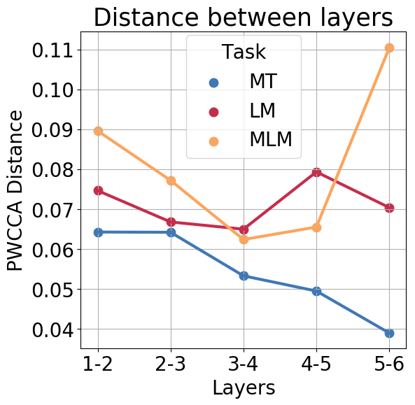
In a similar manner, we measure the difference between representations of consecutive layers in each model (Figure 3(b)). In this case we take views $v^{m,l}$ and $v^{m,l+1}$ and vary layers $l$ and tasks $m$.

For MT, the extent of change monotonically decreases when going from the bottom to top layers, whereas there is no such monotonicity for LM and MLM. This mirrors our view of LM and especially MLM as undergoing phases of encoding and reconstruction (see Section 4.2), thus requiring a stage of dismissing information irrelevant to the output, which, in turn, is accompanied by large changes in the representations between layers.

5.3 Fine-grained analysis

In this section, we select tokens with some predefined property (e.g., frequency) and investigate how much the tokens are influenced by other tokens or how much they influence other tokens.

Amount of change. We measure the extent of change for a group of tokens as the PWCCA distance between the representations of these tokens for a pair of adjacent layers $(l,l+1)$. This quantifies the amount of information the tokens receive in this layer.

Influence. To measure the influence of a token at $l$th layer on other tokens, we measure PWCCA distance between two versions of representations of other tokens in a sentence: first after encoding as usual, second when encoding first $l-1$ layers as usual and masking out the influencing token at the $l$th layer.

5.3.1 Varying token frequency

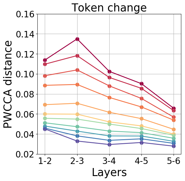
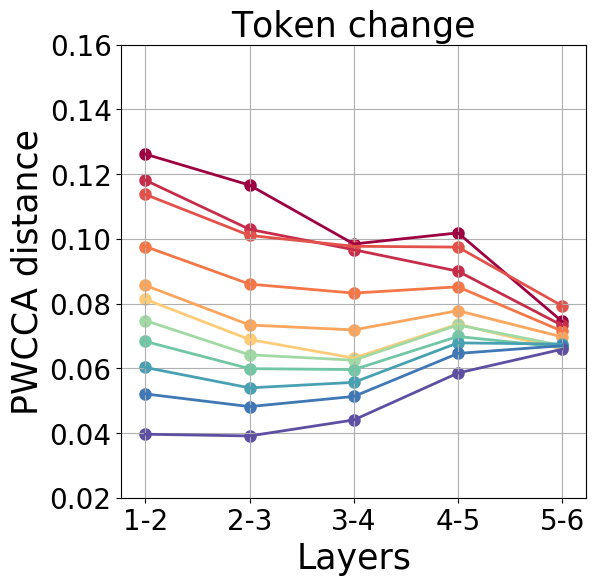
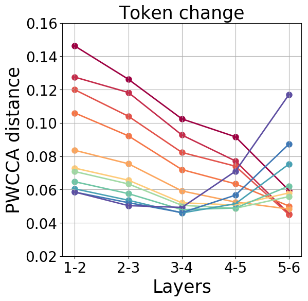
Figure 4 shows a clear dependence of the amount of change on token frequency. Frequent tokens change more than rare ones in all layers in both LM and MT. Interestingly, unlike MT, for LM this dependence dissipates as we move towards top layers. We can speculate that top layers focus on predicting the future rather than incorporating the past, and, at that stage, token frequency of the last observed token becomes less important.

The behavior for MLM is quite different. The two stages for MLMs could already be seen in Figures 1 and 3(b). They are even more pronounced here. The transition from a generalized token representation, formed at the encoding stage, to recreating token identity apparently requires more changes for rare tokens.

(a) MT

(b) LM

(c) MLM

Figure 4: Token change vs its frequency.

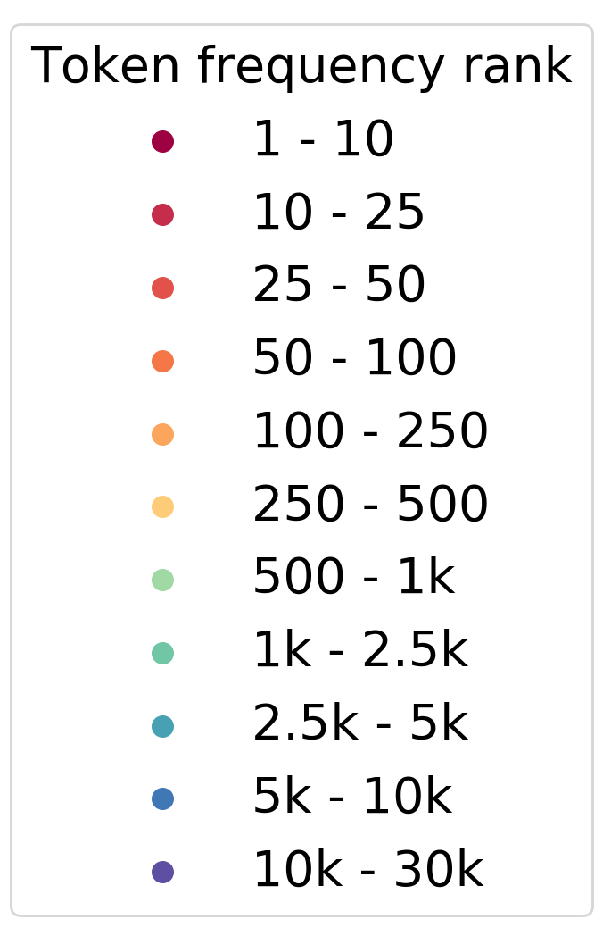
When measuring influence, we find that rare tokens generally influence more than frequent ones (Figure 5). We notice an extreme influence of rare tokens at the first MT layer and at all LM layers. In contrast, rare tokens are not the most influencing ones at the lower layers of MLM. We hypothesize that the training procedure of MLM, with masking out some tokens or replacing them with random ones, teaches the model not to over-rely on these tokens before their context is well understood. To test our hypothesis, we additionally trained MT and LM models with token dropout on the input side (Figure 6). As we expected, there is no extreme influence of rare tokens when using this regularization, supporting the above interpretation.

Interestingly, our earlier study of the MT Transformer Voita et al. (2019) shows how this influence of rare tokens is implemented by the model. In that work, we observed that, for any considered language pair, there is one dedicated attention head in the first encoder layer which tends to point to the least frequent tokens in every sentence. The above analysis suggest that this phenomenon is likely due to overfitting.

(a) MT

(b) LM

(c) MLM

Figure 5: Token influence vs its frequency.

(a) MT

(b) LM

Figure 6: Token influence vs its frequency for models trained with word dropout (in training, each input token is replaced with a random with the probability 10$\%$).

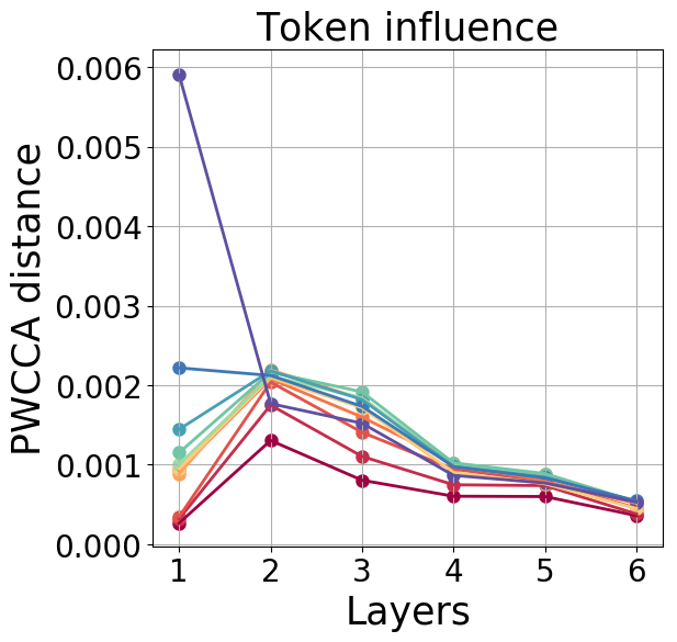
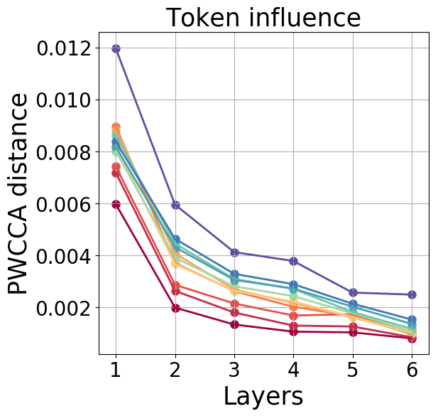
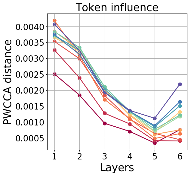
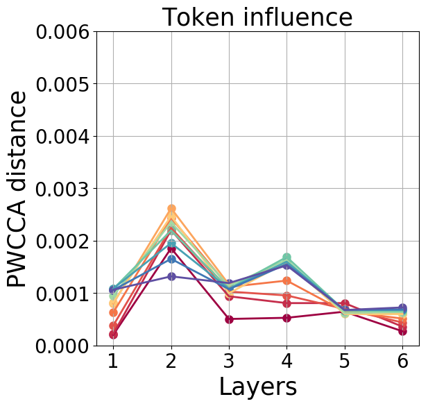
We also analyzed the extent of change and influence splitting tokens according to their part of speech; see appendix for details.

6 What does a layer represent?

Whereas in the previous section we were interested in quantifying the amount of information exchanged between tokens, here we primarily want to understand what representation in each layer ‘focuses’ on. We evaluate to what extent a certain property is important for defining a token representation at each layer by (1) selecting a large number of token occurrences and taking their representations; (2) validating if a value of the property is the same for token occurrences corresponding to the closest representations. Though our approach is different from probing tasks, we choose the properties which will enable us to relate to other works reporting similar behaviour Zhang and Bowman (2018); Blevins et al. (2018); Tenney et al. (2019a). The properties we consider are token identity, position in a sentence, neighboring tokens and CCG supertags.

6.1 Methodology

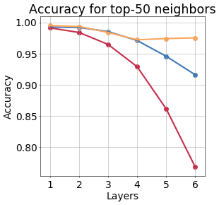
For our analysis, we take 100 random word types from the top 5,000 in our vocabulary. For each word type, we gather 1,000 different occurrences along with the representations from all three models. For each representation, we take the closest neighbors among representations at each layer and evaluate the percentage of neighbors with the same value of the property.

6.2 Preserving token identity and position

In this section, we track the loss of information about token identity (i.e., word type) and position. Our motivation is three-fold. First, this will help us to confirm the results provided on Figure 1; second, to relate to the work reporting results for probing tasks predicting token identity. Finally, the Transformer starts encoding a sentence from a positional and a word embedding, thus it is natural to look at how this information is preserved.

(a)

(b)

Figure 7: Preserving (a) token identity, (b) position

​​​​​	​​​​​	​​​​​​​	​​​​​​​	​​​​​​​	​​​​​​​	​​​​
​​​​​	​​​​​	​​​​​​​	​​​​​​​	​​​​​​​	​​​​​​​	​​​​
​​​​​	​​​​​	​​​​​​​	​​​​​​​	​​​​​​​	​​​​​​​	​​​​

Figure 8: t-SNE of different occurrences of the tokens “is” (red), “are” (orange), “was” (blue), “were” (lightblue). On the x-axis are layers.

6.2.1 Preserving token identity

We want to check to what extent a model confuses representations of different words. For each of the considered words we add 9000 representations of words which potentially could be confused with it. For this extended set of representations, we follow the methodology described above.

Results are presented in Figure 7(a). Reassuringly, the plot is very similar to the one computed with MI estimators (Figure 1), further supporting the interpretations we gave previously (Section 4). Now, let us recall the findings by Zhang and Bowman (2018) regarding the superior performance of untrained LSTMs over trained ones on the task of token identity prediction. They mirror our view of the evolution of a token representation as going through compression and prediction stages, where the learning objective defines the process of forgetting information. If a network is not trained, it is not forced to forget input information.

Figure 8 shows how representations of different occurrences of the words “is”, “are”, “was”, “were” get mixed in MT and LM layers and disambiguated for MLM. For MLM, $15\%$ of tokens were masked as in training. In the first layer, these masked states form a cluster separate from the others, and then they get disambiguated as we move bottom-up across the layers.

6.2.2 Preserving token position

​​​​​	​​​​​	​​​​​​​	​​​​​​​	​​​​​​​	​​​​​​​	​​​​
​​​​​	​​​​​	​​​​​​​	​​​​​​​	​​​​​​​	​​​​​​​	​​​​
​​​​​	​​​​​	​​​​​​​	​​​​​​​	​​​​​​​	​​​​​​​	​​​​

Figure 9: t-SNE of different occurrences of the token “it”, position is in color (the larger the word index the darker its color). On the x-axis are layers.

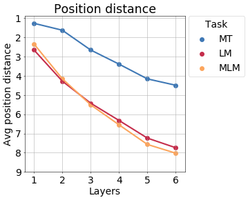
We evaluate the average distance of position of the current occurrence and the top 5 closest representations. The results are provided in Figure 7(b). This illustrates how the information about input (in this case, position), potentially not so relevant to the output (e.g., next word for LM), gets gradually dismissed. As expected, encoding input positions is more important for MT, so this effect is more pronounced for LM and MLM. An illustration is in Figure 9. For MT, even on the last layer ordering by position is noticeable.

6.3 Lexical and syntactic context

In this section, we will look at the two properties: identities of immediate neighbors of a current token and CCG supertag of a current token. On the one hand, these properties represent a model’s understanding of different types of context: lexical (neighboring tokens identity) and syntactic. On the other, they are especially useful for our analysis since they can be split into information about ‘past’ and ‘future’ by taking either left or right neighbor or part of a CCG tag.

6.3.1 The importance of neighboring tokens

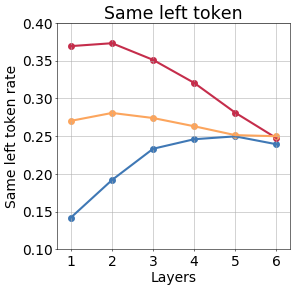
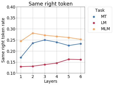
Figure 10 supports our previous expectation that for LM the importance of a previous token decreases, while information about future token is being formed. For MLM, the importance of neighbors gets higher until the second layer and decreases after. This may reflect stages of context encoding and token reconstruction.

(a) left

(b) right

Figure 10: Preserving immediate neighbors

(a)

(b)

(c)

Figure 11: Preserving CCG supertag.

6.3.2 The importance of CCG tags

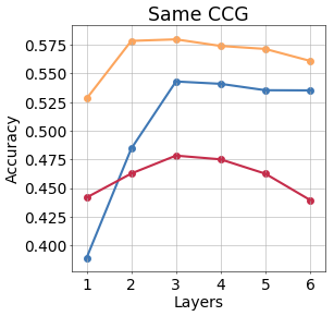
Results are provided in Figure 11(a). As in previous experiments, importance of CCG tag for MLM degrades at higher layers. This agrees with the work by Tenney et al. (2019a). The authors observe that for different tasks (e.g., part-of-speech, constituents, dependencies, semantic role labeling, coreference) the contribution of a layer to a task increases up to a certain layer, but then decreases at the top layers. Our work gives insights into the underlying process defining this behavior.

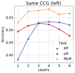
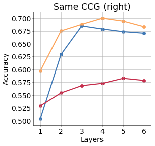
For LM these results are not really informative since it does not have access to the future. We go further and measure importance of parts of a CCG tag corresponding to previous (Figure 11(b)) and next (Figure 11(c)) parts of a sentence. It can be clearly seen that LM first accumulates information about the left part of CCG, understanding the syntactic structure of the past. Then this information gets dismissed while forming information about future.

Figure 12 shows how representations of different occurrences of the token “is” get reordered in the space according to CCG tags (colors correspond to tags).

​​​​​	​​​​​	​​​​​​​	​​​​​​​	​​​​​​​	​​​​​​​	​​​​
​​​​​	​​​​​	​​​​​​​	​​​​​​​	​​​​​​​	​​​​​​​	​​​​
​​​​​	​​​​​	​​​​​​​	​​​​​​​	​​​​​​​	​​​​​​​	​​​​

Figure 12: t-SNE of different occurrences of the token “is”, CCG tag is in color (intensity of a color is a token position). On the x-axis are layers.

7 Additional related work

Previous work analyzed representations of MT and/or LM models by using probing tasks. Different levels of linguistic analysis have been considered including morphology Belinkov et al. (2017a); Dalvi et al. (2017); Bisazza and Tump (2018), syntax Shi et al. (2016); Tenney et al. (2019b) and semantics Hill et al. (2017); Belinkov et al. (2017b); Raganato and Tiedemann (2018); Tenney et al. (2019b). Our work complements this line of research by analyzing how word representations evolve between layers and gives insights into how models trained on different tasks come to represent different information.

Canonical correlation analysis has been previously used to investigate learning dynamics of CNNs and RNNs, to measure the intrinsic dimensionality of layers in CNNs and compare representations of networks which memorize and generalize Raghu et al. (2017); Morcos et al. (2018). Bau et al. (2019) used SVCCA as one of the methods used for identifying important individual neurons in NMT models. Saphra and Lopez (2019) used SVCCA to investigate how representations of linguistic structure are learned over time in LMs.

8 Conclusions

In this work, we analyze how the learning objective determines the information flow in the model. We propose to view the evolution of a token representation between layers from the compression/prediction trade-off perspective. We conduct a series of experiments supporting this view and propose a possible explanation for superior performance of MLM over LM for pretraining. We relate our findings to observations previously made in the context of probing tasks.

Appendix A Data and Setting

A.1 Model architecture

For machine translation models, we follow the setup of the Transformer base model Vaswani et al. (2017). More precisely, the number of layers in the encoder and in the decoder is $N=6$. We use $h=8$ parallel attention layers, i.e. heads. The dimensionality of input and output is $d_{model}=512$, and the inner-layer of the feed-forward networks has the dimensionality $d_{ff}=2048$. For language models, we use only the encoder of the model (with the same hyper-parameters).

A.2 Training

Sentences were encoded using byte-pair encoding Sennrich et al. (2016), with source and target vocabularies of about 32000 tokens. Source vocabulary is the same for all tasks. Minibatch size is set to approximately 15000 source tokens. Training examples were batched together by approximate sequence length. Each training batch contained a set of translation pairs, approximately 15000 source tokens each. The optimizer and learning rate schedule we use are the same as in Vaswani et al. (2017). Since using a large number of training steps was reported to be important for the MLM objective, we follow Devlin et al. (2018) and train MLM for 1 million training steps and other models till convergence.

Appendix B Fine-grained analysis of change and influence: varying PoS

Figure 13 shows the amount of change for different parts of speech, Figure 14 – the amount of influence for different parts of speech. Generally, the patterns are similar to the ones for frequency groups: parts of speech with frequent tokens (preposition, conjunction, etc.) change more and influence less.

(a) MT

(b) LM

(c) MLM

Figure 13: Token change vs its part of speech.

(a) MT

(b) LM

(c) MLM

Figure 14: Token influence vs its part of speech.

Appendix C What does a layer represent?

C.1 Preserving token identity: experimental setup

In this section, we want to check to what extent a model confuses representations of different tokens. For each of the selected tokens described above (“main” tokens), we pick tokens which potentially could be confused with the token under consideration (“contrastive” tokens). In our setting, contrastive tokens are the top 10 closest tokens in the embedding space (separately for each model). For example, tokens “is”, “are”, “was”, “were” are close in the embedding space of each of the models. Then for each main token we gather representations of 9000 different occurrences of its contrastive tokens, and add them to the 1000 states of the main token. All in all, we get 200 groups of representations; each group contains representations of 1000 occurrences of the main token and 9000 of the contrastive ones (at each layer). For representations of the main token in a group, we measure the average percentage of representations of the same token for top closest among 10000 representations.

References

- Bau et al. (2019) Anthony Bau, Yonatan Belinkov, Hassan Sajjad, Nadir Durrani, Fahim Dalvi, and James Glass. 2019. Identifying and controlling important neurons in neural machine translation. In International Conference on Learning Representations, New Orleans.
- Belinkov et al. (2017a) Yonatan Belinkov, Nadir Durrani, Fahim Dalvi, Hassan Sajjad, and James Glass. 2017a. What do neural machine translation models learn about morphology? In Proceedings of the 55th Annual Meeting of the Association for Computational Linguistics (Volume 1: Long Papers), pages 861–872. Association for Computational Linguistics.
- Belinkov et al. (2017b) Yonatan Belinkov, Lluís Màrquez, Hassan Sajjad, Nadir Durrani, Fahim Dalvi, and James Glass. 2017b. Evaluating layers of representation in neural machine translation on part-of-speech and semantic tagging tasks. In Proceedings of the Eighth International Joint Conference on Natural Language Processing (Volume 1: Long Papers), pages 1–10. Asian Federation of Natural Language Processing.
- Bisazza and Tump (2018) Arianna Bisazza and Clara Tump. 2018. The lazy encoder: A fine-grained analysis of the role of morphology in neural machine translation. In Proceedings of the 2018 Conference on Empirical Methods in Natural Language Processing, pages 2871–2876, Brussels, Belgium. Association for Computational Linguistics.
- Blevins et al. (2018) Terra Blevins, Omer Levy, and Luke Zettlemoyer. 2018. Deep RNNs encode soft hierarchical syntax. In Proceedings of the 56th Annual Meeting of the Association for Computational Linguistics (Volume 2: Short Papers), pages 14–19, Melbourne, Australia. Association for Computational Linguistics.
- Bojar et al. (2018) Ondřej Bojar, Christian Federmann, Mark Fishel, Yvette Graham, Barry Haddow, Matthias Huck, Philipp Koehn, and Christof Monz. 2018. Findings of the 2018 conference on machine translation (wmt18). In Proceedings of the Third Conference on Machine Translation, Volume 2: Shared Task Papers, pages 272–307, Belgium, Brussels. Association for Computational Linguistics.
- Dalvi et al. (2017) Fahim Dalvi, Nadir Durrani, Hassan Sajjad, Yonatan Belinkov, and Stephan Vogel. 2017. Understanding and improving morphological learning in the neural machine translation decoder. In Proceedings of the Eighth International Joint Conference on Natural Language Processing (Volume 1: Long Papers), pages 142–151. Asian Federation of Natural Language Processing.
- Devlin et al. (2018) Jacob Devlin, Ming-Wei Chang, Kenton Lee, and Kristina Toutanova. 2018. Bert: Pre-training of deep bidirectional transformers for language understanding. arXiv preprint arXiv:1810.04805.
- Hill et al. (2017) Felix Hill, Kyunghyun Cho, Sébastien Jean, and Y Bengio. 2017. The representational geometry of word meanings acquired by neural machine translation models. Machine Translation, 31.
- Hotelling (1936) Harold Hotelling. 1936. Relations between two sets of variates. Biometrika, 28:321–337.
- Lample and Conneau (2019) Guillaume Lample and Alexis Conneau. 2019. Cross-lingual language model pretraining. arXiv preprint arXiv:1901.07291.
- Manning et al. (2014) Christopher D. Manning, Mihai Surdeanu, John Bauer, Jenny Finkel, Steven J. Bethard, and David McClosky. 2014. The Stanford CoreNLP natural language processing toolkit. In Proceedings of 52nd Annual Meeting of the Association for Computational Linguistics: System Demonstrations, pages 55–60, Baltimore, Maryland. Association for Computational Linguistics.
- Morcos et al. (2018) Ari S. Morcos, Maithra Raghu, and Samy Bengio. 2018. Insights on representational similarity in neural networks with canonical correlation. In NeurIPS, Montreal, Canada.
- Niehues et al. (2018) Jan Niehues, Ronaldo Cattoni, Sebastian Stüker, Mauro Cettolo, Marco Turchi, and Marcello Federico. 2018. The IWSLT 2018 Evaluation Campaign. In Proceedings of the 15th International Workshop on Spoken Language Translation, pages 118–123, Bruges, Belgium.
- Paninski (2003) Liam Paninski. 2003. Estimation of entropy and mutual information. Neural computation, 15(6):1191–1253.
- Peters et al. (2018) Matthew Peters, Mark Neumann, Mohit Iyyer, Matt Gardner, Christopher Clark, Kenton Lee, and Luke Zettlemoyer. 2018. Deep contextualized word representations. In Proceedings of the 2018 Conference of the North American Chapter of the Association for Computational Linguistics: Human Language Technologies, Volume 1 (Long Papers), pages 2227–2237, New Orleans, Louisiana. Association for Computational Linguistics.
- Radford et al. (2018) Alec Radford, Karthik Narasimhan, Tim Salimans, and Ilya Sutskever. 2018. Improving language understanding by generative pre-training.
- Raganato and Tiedemann (2018) Alessandro Raganato and Jörg Tiedemann. 2018. An analysis of encoder representations in transformer-based machine translation. In Proceedings of the 2018 EMNLP Workshop BlackboxNLP: Analyzing and Interpreting Neural Networks for NLP, pages 287–297, Brussels, Belgium. Association for Computational Linguistics.
- Raghu et al. (2017) Maithra Raghu, Justin Gilmer, Jason Yosinski, and Jascha Sohl-Dickstein. 2017. Svcca: Singular vector canonical correlation analysis for deep learning dynamics and interpretability. In NeurIPS, Los Angeles.
- Sajjadi et al. (2018) Mehdi S. M. Sajjadi, Olivier Bachem, Mario Lucic, Olivier Bousquet, and Sylvain Gelly. 2018. Assessing generative models via precision and recall. In Advances in Neural Information Processing Systems 31, pages 5228–5237.
- Saphra and Lopez (2019) Naomi Saphra and Adam Lopez. 2019. Understanding learning dynamics of language models with SVCCA. In Proceedings of the 2019 Conference of the North American Chapter of the Association for Computational Linguistics: Human Language Technologies, Volume 1 (Long and Short Papers), pages 3257–3267, Minneapolis, Minnesota. Association for Computational Linguistics.
- Sennrich et al. (2016) Rico Sennrich, Barry Haddow, and Alexandra Birch. 2016. Neural machine translation of rare words with subword units. In Proceedings of the 54th Annual Meeting of the Association for Computational Linguistics (Volume 1: Long Papers), pages 1715–1725, Berlin, Germany. Association for Computational Linguistics.
- Shi et al. (2016) Xing Shi, Inkit Padhi, and Kevin Knight. 2016. Does string-based neural mt learn source syntax? In Proceedings of the 2016 Conference on Empirical Methods in Natural Language Processing, pages 1526–1534. Association for Computational Linguistics.
- Shwartz-Ziv and Tishby (2017) Ravid Shwartz-Ziv and Naftali Tishby. 2017. Opening the black box of deep neural networks via information. arXiv preprint arXiv:1703.00810.
- Tenney et al. (2019a) Ian Tenney, Dipanjan Das, and Ellie Pavlick. 2019a. BERT rediscovers the classical NLP pipeline. In Proceedings of the 57th Annual Meeting of the Association for Computational Linguistics, pages 4593–4601, Florence, Italy. Association for Computational Linguistics.
- Tenney et al. (2019b) Ian Tenney, Patrick Xia, Berlin Chen, Alex Wang, Adam Poliak, R Thomas McCoy, Najoung Kim, Benjamin Van Durme, Samuel R Bowman, Dipanjan Das, et al. 2019b. What do you learn from context? probing for sentence structure in contextualized word representations. In International Conference on Learning Representations.
- Tishby et al. (1999) Naftali Tishby, Fernando C Pereira, and William Bialek. 1999. The information bottleneck method. In Proceedings of the 37-th Annual Allerton Conference on Communication, Control and Computing, pages 368–377.
- Tishby and Zaslavsky (2015) Naftali Tishby and Noga Zaslavsky. 2015. Deep learning and the information bottleneck principle. 2015 IEEE Information Theory Workshop (ITW), pages 1–5.
- Vaswani et al. (2017) Ashish Vaswani, Noam Shazeer, Niki Parmar, Jakob Uszkoreit, Llion Jones, Aidan N Gomez, Lukasz Kaiser, and Illia Polosukhin. 2017. Attention is all you need. In Advances in Neural Information Processing Systems 30, pages 5998–6008, Los Angeles.
- Voita et al. (2019) Elena Voita, David Talbot, Fedor Moiseev, Rico Sennrich, and Ivan Titov. 2019. Analyzing multi-head self-attention: Specialized heads do the heavy lifting, the rest can be pruned. In Proceedings of the 57th Annual Meeting of the Association for Computational Linguistics, pages 5797–5808, Florence, Italy. Association for Computational Linguistics.
- Yoshikawa et al. (2017) Masashi Yoshikawa, Hiroshi Noji, and Yuji Matsumoto. 2017. A* CCG parsing with a supertag and dependency factored model. In Proceedings of the 55th Annual Meeting of the Association for Computational Linguistics (Volume 1: Long Papers), pages 277–287, Vancouver, Canada. Association for Computational Linguistics.
- Zhang and Bowman (2018) Kelly Zhang and Samuel Bowman. 2018. Language modeling teaches you more than translation does: Lessons learned through auxiliary syntactic task analysis. In Proceedings of the 2018 EMNLP Workshop BlackboxNLP: Analyzing and Interpreting Neural Networks for NLP, pages 359–361, Brussels, Belgium. Association for Computational Linguistics.