Galaxy disc scaling relations: A tight linear galaxy–halo connection challenges abundance matching

In $\Lambda$CDM cosmology, to first order, galaxies form out of the cooling of baryons within the virial radius of their dark matter halo. The fractions of mass and angular momentum retained in the baryonic and stellar components of disc galaxies put strong constraints on our understanding of galaxy formation. In this work, we derive the fraction of angular momentum retained in the stellar component of spirals, $f_{j}$, the global star formation efficiency $f_{M}$, and the ratio of the asymptotic circular velocity ($V_{\rm flat}$) to the virial velocity $f_{V}$, and their scatter, by fitting simultaneously the observed stellar mass-velocity (Tully-Fisher), size-mass, and mass-angular momentum (Fall) relations. We compare the goodness of fit of three models: (i) where the logarithm of $f_{j}$, $f_{M}$, and $f_{V}$ vary linearly with the logarithm of the observable $V_{\rm flat}$; (ii) where these values vary as a double power law; and (iii) where these values also vary as a double power law but with a prior imposed on $f_{M}$ such that it follows the expectations from widely used abundance matching models. We conclude that the scatter in these fractions is particularly small ($\sim 0.07$ dex) and that the “linear” model is by far statistically preferred to that with abundance matching priors. This indicates that the fundamental galaxy formation parameters are small-scatter single-slope monotonic functions of mass, instead of being complicated non-monotonic functions. This incidentally confirms that the most massive spiral galaxies should have turned nearly all the baryons associated with their haloes into stars. We call this the failed feedback problem.

1 Introduction

The current $\Lambda$ cold dark matter ($\Lambda$CDM) cosmological model is very successful at reproducing observations of the large-scale structure of the Universe. However, galactic scales still present to this day a number of interesting challenges for our understanding of structure formation in such a cosmological context (e.g. Bullock & Boylan-Kolchin 2017). These challenges could have important consequences on our understanding of the interplay between baryons and dark matter, or even on the roots of the cosmological model itself, including the very nature of dark matter. For instance, the most inner parts of galaxy rotation curves present a wide variety of shapes (Oman et al. 2015, 2019), which might be indicative of a variety of central dark matter profiles ranging from cusps to cores and closely related to the observed central surface density of baryons (e.g. Lelli et al. 2013, 2016c; Ghari et al. 2019). In addition to such surprising central correlations, the phenomenology of global galactic scaling laws, which relate fundamental galactic structural parameters of both baryons and dark matter, also carries important clues that should inform us about the galaxy formation process in a cosmological context.

Given the complexity of the baryon physics leading to the formation of galaxies, which involves for instance gravitational instabilities, gas dissipation, mergers and interactions with neighbours, or feedback from strong radiative sources, it is remarkable that many of the most basic structural scaling relations of disc galaxies are simple, tight power laws (see e.g. van der Kruit & Freeman 2011, for a review); these most basic structural scaling relations, for example, can be between the stellar or baryonic mass of the galaxy and its rotational velocity (Tully & Fisher 1977; Lelli et al. 2016b), its stellar mass and size (Kormendy 1977; Lange et al. 2016), and its stellar mass and stellar specific angular momentum (Fall 1983; Posti et al. 2018a).

The interplay of all the complex phenomena involved in the galaxy formation process thus conspires to produce a population of galaxies which is, to first order, simply rescalable. Interestingly, in $\Lambda$CDM, dark matter haloes also follow simple, tight, power-law scaling relations and their structure is fully rescalable. Thus, all of this is suggestive of the existence of a simple correspondence between the scaling relations of dark matter haloes and galaxies (e.g. Posti et al. 2014). In this context, we can consider to first order a simplified picture in which galaxies form out of the cooling of baryons within the virial radius of their dark matter halo. That is, before any dissipation happens, the fraction of total matter that is baryonic inside newly formed haloes would not differ on average from the current value of the cosmic baryon fraction $f_{\rm b}\equiv\Omega_{\rm b}/\Omega_{\rm m}\simeq 0.157$, where $\Omega_{\rm b}$ and $\Omega_{\rm m}$ are the baryonic and total matter densities of the Universe, respectively (Planck Collaboration et al. 2018). In this simplified picture, galaxies are then formed out of those baryons that effectively dissipate and sink towards the centre of the potential well, and the final structural properties of galaxies, such as mass, size, and angular momentum, are then directly related to the interplay between the (cooling) baryons and (dissipationless) dark matter.

Observationally proving that indeed the masses, sizes, and angular momenta of galaxies are simply and directly proportional to those of their dark matter haloes, would be a major finding. This means that, out of all the complexity of galaxy formation in a cosmological context, a fundamental regularity is still emerging, which we would then need to understand. Some of the earliest and most influential theoretical models of disc galaxy formation relied on reproducing the observed scaling laws of discs to constrain their free parameters (e.g. Fall & Efstathiou 1980; Dalcanton et al. 1997; Mo et al. 1998). These parameters are often chosen to be physically meaningful and fundamental quantities that synthetically encode galaxy formation, such as a global measure of the efficiency at forming stars from the cooling material (e.g. Behroozi et al. 2013; Moster et al. 2013, hereafter M+13) or a measure of the net gains or losses of the total angular momentum from that initially acquired via tidal torques (Peebles 1969; Romanowsky & Fall 2012; Pezzulli et al. 2017). The rich amount of data collected in recent years for spiral galaxies both in the nearby Universe and at high redshift allows an unprecedented exploitation of the observed scaling laws which, when fitted simultaneously, can yield very strong constraints on such fundamental galaxy formation parameters (e.g. Dutton et al. 2007; Dutton & van den Bosch 2012; Desmond & Wechsler 2015; Lapi et al. 2018).

While being the focus of many studies over the past years, the connection between galaxy and halo properties is still not trivial to measure observationally (see Wechsler & Tinker 2018, for a recent review). However, arguably the most important bit of this connection, the relation between galaxy stellar mass and dark matter halo mass, is very well studied and the results from different groups tend to converge towards a complex, non-linear correspondence. As long as galaxies of all types are considered and stacked together, the same non-linear relation, with a break at around $L^{\ast}$ galaxies, is found irrespective of the different observations used to probe this relation: for instance, the match of the halo mass function to the observed stellar mass function (the so-called abundance matching ansatz; e.g. Vale & Ostriker 2004; Kravtsov et al. 2004; Behroozi et al. 2013; M+13), galaxy clustering (e.g. Zheng et al. 2007), group catalogues (e.g. Yang et al. 2008), weak galaxy-galaxy lensing (e.g. Mandelbaum et al. 2006; Leauthaud et al. 2012; van Uitert et al. 2016), and satellite kinematics (van den Bosch et al. 2004; More et al. 2011; Wojtak & Mamon 2013). Hence, this would imply that the high regularity of the observed disc scaling laws is not a direct reflection of the rescalability of dark matter haloes. If the stellar-to-halo mass relation of disc galaxies is non-linear, then the relation between disc rotation velocity and halo virial velocity (Navarro & Steinmetz 2000; Cattaneo et al. 2014; Ferrero et al. 2017), as well as the relation between stellar and halo specific angular momenta (Shi et al. 2017; Posti et al. 2018b), also have to be highly non-linear.

Nonetheless, recently Posti et al. (2019, hereafter PFM19) measured individual halo masses for a large sample of nearby disc galaxies, from small dwarfs to spirals $\sim 10$ times more massive than the Milky Way. These authors used accurate near-infrared (3.6 $\mu$m) photometry with the Spitzer Space Telescope and HI interferometry (Lelli et al. 2016a) to determine the stellar and dark matter halo masses robustly, by means of fitting the observed gas rotation curves. Surprisingly, the authors found no indication of a break in the stellar-to-halo mass relation of their sample of spirals. This finding is in significant tension with expectations of abundance matching models for galaxies with stellar masses above $8\times 10^{10}M_{\odot}$ (see also McGaugh et al. 2010). Since the high-mass slope of the stellar-to-halo mass relation is commonly understood in terms of strong central feedback (e.g. Wechsler & Tinker 2018), we call this observational discrepancy the failed feedback problem. This discrepancy might be there simply as a result of a morphology-dependent galaxy-halo connection. While the relation found by PFM19 applies to disc galaxies, the stellar-to-halo mass relation from abundance matching instead is an average statistic derived for galaxies of all types that is heavily dominated by spheroids at the high-mass end. This would imply that the galaxy-halo connection for discs and spheroids can be significantly different, for example it could be linear for discs while being highly non-linear for spheroids.

If this is the case for disc galaxies in the nearby Universe, then this should leave a measurable imprint on their structural scaling laws, such as the Tully-Fisher, size-mass, and Fall relations. It is possible to model these three scaling laws (of which the last two are dependent) with three (dependent) fundamental galaxy formation parameters: one to determine the stellar-to-halo mass relation, one for the stellar-to-halo specific angular momentum relation, and one for the disc-to-virial rotation velocity relation. The shape of the observed scaling laws carries enough information to constrain these three quantities and their scatter together simultaneously, and to disentangle whether a simple, linear galaxy–halo correspondence is preferred for spirals or if a more complex, non-linear correspondence is needed (e.g. Lapi et al. 2018).

In this paper we use individual, high-quality measurements of the photometry and gas rotation velocity of a wide sample of nearby spiral galaxies, from the smallest dwarfs to the most massive giant spirals, to fit their observed scaling relations with analytic galaxy formation models that depend on the three fundamental parameters mentioned above. We perform fits of models with either i) a simple, linear galaxy–halo correspondence, ii) a more complex, non-linear correspondence, and iii) also a complex, non-linear correspondence that has an additional prior on the stellar-to-halo mass relation from popular abundance matching models. We then statistically evaluate the goodness of fit in all three cases and, finally, we compare the outcomes of these three cases with the halo masses recently measured from the rotation curves of the same spirals; thus, we have additional and independent information on which of the models we tried is more realistic.

The paper is organised as follows. In Section 2 we describe the dataset that we use; in Section 3 we introduce the analytic models that we adopt to fit the observed scaling relations and our fitting technique; in Section 4 we present the fitting results, the predictions of the models, and the a posteriori comparison with the halo masses measured from the rotation curve decompositions; in Section 5 we summarise and discuss the implications of our findings.

Throughout the paper we use a fixed critical overdensity parameter $\Delta=200$ to define dark matter haloes and the standard $\Lambda$CDM model, which has the following parameters estimated by the Planck Collaboration et al. (2018): $f_{\rm b}\equiv\Omega_{\rm b}/\Omega_{\rm m}\simeq 0.157$ and $H_{0}=67.4$ km s^-1 Mpc^-1.

2 Data

2.1 SPARC

Our primary data catalogue comes from the sample of 175 nearby disc galaxies with near-infrared photometry and HI rotation curves (SPARC) collected by Lelli et al. (2016a, hereafter LMS16). These galaxies span more than 4 orders of magnitude in luminosity at 3.6 $\mu$m and all morphological types, from irregulars to lenticulars. The sample was primarily collected for studies of high-quality, regular, and extended rotation curves; thus galaxies have been primarily selected on the basis of interferometric radio data. Moreover, the catalogue selection has been refined to include only galaxies with near-infrared photometry from the Spitzer Space Telescope. Hence, even though it is not volume limited, this sample provides a fair representation of the full population of nearby (regularly rotating) spirals. Samples of spirals with a much higher completeness and with high-quality HI kinematics will soon be available with the Square Kilometre Array precursors and pathfinders, such as MeerKAT or APERture Tile In Focus (APERTIF).

In what follows we consider only galaxies with inclinations larger than $30^{\circ}$, since for nearly face-on spirals the rotation curves are highly uncertain. This introduces no biases, since discs are randomly orientated with respect to the line of sight.

We used the gas rotation velocity along the flat part of the rotation curve as a representative velocity for the system because it is known to minimise the scatter of the (baryonic) Tully-Fisher relation (e.g. Verheijen 2001; Lelli et al. 2019). We used the same estimate of $V_{\rm flat}$ as in Lelli et al. (2016b), which is basically an average of the three last measured points of the rotation curve, with the condition that the curve is flat within $\sim 5\%$ over these last three points. When fitting the models in the following sections, we only consider the sample of galaxies that satisfies this condition; this includes 125 galaxies. We nonetheless show the locations on the scaling relations of the other 33 galaxies (with inclinations larger than $30^{\circ}$) that do not satisfy that criterion (white filled circles); also for these objects we adopted the definition of $V_{\rm flat}$ and its uncertainty from Lelli et al. (2016b).

The disc scale lengths $R_{\rm d}$ have also been derived by Lelli et al. (2016a) with exponential fits to the outer parts of the measured surface brightness at 3.6 $\mu$m with Spitzer. These authors did this to exclude the contamination from the bulge (if present) in the central regions of the galaxy. We computed the stellar masses $M_{\star}$ by integrating the observed surface brightness profiles, which are decomposed into a disc and bulge component as in Lelli et al. (2016a), and by assuming a constant mass-to-light ratio for the two components of $(M/L_{\rm disc}^{[3/6]},M/L_{\rm bulge}^{[3/6]})=(0.5,0.7)$. We justified this choice by stellar population synthesis models (e.g. Schombert & McGaugh 2014) and is found to minimise the scatter of the (baryonic) Tully-Fisher (Lelli et al. 2016b; Ponomareva et al. 2018). Moreover, these values are similar to those obtained from the mass decomposition of the rotation curves (Katz et al. 2017, PFM19).

The $j_{\star}-M_{\star}$ relation, aka the Fall relation, is now very well established observationally. Several independent measurements now agree perfectly both on the slope and normalisation of this relation at least for spirals (Romanowsky & Fall 2012; Obreschkow & Glazebrook 2014; Posti et al. 2018a; Fall & Romanowsky 2013, 2018). The total specific angular momentum of the stellar disc is, instead, measured as in Posti et al. (2018a). Given the stellar rotation curve $V_{\star}$, estimated from the HI rotation curve, and the stellar surface density $\Sigma_{\star}$, we calculated

$$j_{\star}=\frac{\int{\rm d}R\,R^{2}\,\Sigma_{\star}(R)\,V_{\star}(R)}{\int{\rm d}R\,R\,\Sigma_{\star}(R)}.$$ (1)

We used this measurement (and associated uncertainty as given by Eq. 3 in Posti et al. 2018a) for the 92 SPARC galaxies with “converged” cumulative $j_{\star}$ profiles, meaning that they flatten in the outskirts to within $\sim 10\%$ (following the definition by Posti et al. 2018a). For the other 33 galaxies with flat rotation curves, but with non-converged cumulative $j_{\star}$ profiles, we adopted the much simpler estimator (see e.g. Romanowsky & Fall 2012)

$$j_{\star}=2\,R_{\rm d}\,V_{\rm flat},$$ (2)

which comes from Eq. (1) under the assumption of an exponential stellar surface density profile with a flat rotation curve. In this equation, we are implicitly assuming that the gas rotation, $V_{\rm flat}$, is a reasonable proxy for the rotation velocity of stars, at least in the outer regions of discs. Stars are indeed found on almost circular orbits in the regularly rotating discs analysed in this work (Iorio et al. 2017; Posti et al. 2018a). The simple $j_{\star}$ estimator in Eq. (2) is widely used and known to be reasonably accurate for spirals, provided that the measurements of $R_{\rm d}$ and $V_{\rm flat}$ are sound (e.g. Fall & Romanowsky 2018). In particular, Posti et al. (2018a), studying the sample of 92 SPARC galaxies with converged profiles, determined that the estimator (2) is unbiased and yields a typical uncertainty of $30-40\%$ on the true $j_{\star}$. Thus, in what follows, we also consider $j_{\star}$ measurements obtained with Eq. (2) and with an uncertainty of $40\%$ for the 33 SPARC galaxies with flat rotation curves, but non-converged cumulative $j_{\star}$ profiles.

2.2 LITTLE THINGS

We added a sub-sample of galaxies drawn from the Local Irregulars That Trace Luminosity Extremes, The HI Nearby Galaxy Survey Survey (LITTLE THINGS, Hunter et al. 2012) to the catalogue described above. These are 17 dwarf irregulars that have fairly regular HI kinematics and are seen at inclinations larger than $30^{\circ}$.

This sample has been recently analysed by Iorio et al. (2017) who determined the rotation curve of each system from the detailed 3D modelling of the HI data. We used their results and applied the same criterion on the rotation curve flatness as for the SPARC sample. We found that 4 out of 17 galaxies (CVnIdwA, DDO53, DDO210, UGC8508) have rotation curves which do not flatten to within $\sim 5\%$ over the last three data points, and thus we excluded these galaxies from the fits but we still show these in the plots (as white filled diamonds).

We determined the size of these galaxies from their optical R-band or V-band images using publicly available data from 1-2 meter class telescopes at the Kitt Peak National Observatory (KPNO; Cook et al. 2014). In the cases where no KPNO data were available, we used Sloan Digital Sky Survey (SDSS) data (CVnIdwA, DDO 101, DDO 47, and DDO 52; Baillard et al. 2011) or Vatican Advanced Technology Telescope (VATT) data (UGC 8508; Taylor et al. 2005) instead. While a number of LITTLE THINGS systems come with IRAC Spitzer images, these are vastly contaminated by bright point-like sources that we found difficult to treat properly. Also considering the superior quality of the optical data, we decided to use the latter for our size measurements.

Using these images, we derived the surface brightness profiles for all 17 systems following the procedure fully described in Marasco et al. (2019), adopting as galaxy centres, inclinations and position angles the values determined by Iorio et al. (2017). We then fit these profiles with exponential functions to determine the galaxy scale lengths, which we found to be in excellent agreement with those inferred by Hunter & Elmegreen (2006). In Figure 1 we illustrate the procedure we use for the representative case of DDO 52. Finally, for the LITTLE THINGS galaxies we used the estimator (2) for the stellar specific angular momentum with a conservative error bar of $40\%$.

3 Model

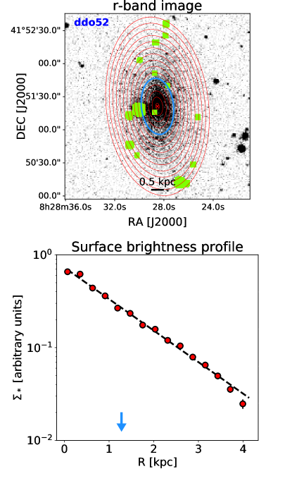
Figure 1: Photometry for DDO 52 as a representative example for the LITTLE THINGS galaxies. Top panel: r-band image with the concentric ellipses showing the annuli where the surface brightness is computed. The green regions are foreground sources that we mask during the derivation of the profile. The blue ellipse is drawn at the disc scale length. Bottom panel: surface brightness profile, normalised to the total light within the outermost ring. The thick dashed black line indicates the exponential fit, while the blue arrow indicates the exponential scale length.

3.1 Dark matter haloes

We started with dark matter haloes, which are described by their structural properties – mass ($M_{\rm h}$), radius ($R_{\rm h}$), velocity ($V_{\rm h}$), and specific angular momentum ($j_{\rm h}$) – defined in an overdensity of $\Delta$ times the critical density of the Universe. Haloes, then, adhere to the following scaling laws (e.g. Mo et al. 2010):

$$M_{\rm h}=\frac{1}{GH}\sqrt{\frac{2}{\Delta}}V_{\rm h}^{3};$$ (3)

$$R_{\rm h}=\frac{1}{H}\sqrt{\frac{2}{\Delta}}V_{\rm h};$$ (4)

$$j_{\rm h}=\frac{2\lambda}{H\sqrt{\Delta}}V_{\rm h}^{2},$$ (5)

where $G$ is the gravitational constant and $\lambda=j_{\rm h}/\sqrt{2}R_{\rm h}V_{\rm h}$ is the halo spin parameter, as in the definition by Bullock et al. (2001, which is conceptually equivalent to the classic definition in ). The distribution of $\lambda$ for $\Lambda$CDM haloes is very well studied and it is known to have a nearly log-normal shape – with mean $\log\overline{\lambda}\approx-1.456$ and scatter $\sigma_{\log\lambda}\approx 0.22$ dex – irrespective of halo mass. Henceforth, since $\lambda$ is not a function of $V_{\rm h}$, Eq. (5) is a simple power law $j_{\rm h}\propto V_{\rm h}^{2}$, while also Eq. (3)-(4) are obviously similar power laws.

3.2 Galaxy formation parameters

We very simply parametrise the intrinsically complex processes of galaxy formation, by considering that, to first order, galaxies form out of the cooling of baryons within the virial radius of their halo. The fundamental parameters we consider are then the following fractions:

$$f_{M}\equiv\frac{M_{\star}}{M_{\rm h}};\qquad f_{j}\equiv\frac{j_{\star}}{j_{\rm h}};\qquad f_{V}\equiv\frac{V_{\rm flat}}{V_{\rm h}};\qquad f_{R}\equiv\frac{R_{\rm d}}{R_{\rm h}}.$$ (6)

The aim of this work is to unveil the galaxy–halo connection constraining and characterising the four galaxy formation fractions above using the observed global properties of disc galaxies.

• The first, and arguably most important, of these parameters is the stellar mass fraction $f_{M}$, which is also sometimes loosely referred to as global star formation efficiency parameter (e.g. Behroozi et al. 2013; M+13). This describes how much of the hot gas associated with the dark matter halo was able to cool and to form stars throughout the lifetime of the galaxy. Thus, in a very broad sense, this encapsulates the average efficiency of gas-to-stars conversion integrated over time. On average, this parameter has an obvious strict upper limit set by the cosmic baryon fraction $f_{\rm b}\simeq 0.157$.

• The second is the specific angular momentum fraction $f_{j}$, also known as the retained fraction of angular momentum (e.g. Romanowsky & Fall 2012). After the halo collapsed, but before galaxy formation started, tidal torques supplied baryons and dark matter with nearly equal amounts of angular momentum, so $j_{\rm baryon}/j_{\rm h}=1$ (e.g. Fall & Efstathiou 1980). Stars, however, form from some fraction of these baryons, whose final angular momentum distribution is the product of the interplay of several physical processes (e.g. cooling, mergers, and feedback, gas cycles). This results in an $f_{j}$ that can easily deviate from unity.

• The third is the velocity fraction $f_{V}$, which is the ratio of the circular velocity at the edge of the galactic disc to that at the virial radius. While this factor in principle can take any value depending on the galaxy and halo mass distribution, but also depending on the extension of the measured rotation curve, it is typically expected to be $f_{V}\gtrsim 1$ for large and well resolved galaxies ($\log M_{\star}/M_{\odot}>9$, see e.g. Papastergis et al. 2011).

• The last parameter is the size fraction $f_{R}$, i.e. the ratio of the disc exponential scale length ($R_{\rm d}$) to the halo virial radius ($R_{\rm h}$). However, if we assume that the size of the galaxy is regulated by its angular momentum (Fall & Efstathiou 1980; Mo et al. 1998; Kravtsov 2013), then $f_{j}$ and $f_{R}$ are not independent. It is easy to work out their relation as a function of the dark matter halo profile, which turns out to be analytic in the case of an exponential disc with a flat rotation curve (see Appendix A), i.e.,

  $$f_{R}=\frac{\lambda}{\sqrt{2}}\frac{f_{j}}{f_{V}}.$$ (7)

  An analogous result was already derived analytically by Fall (1983). For more realistic haloes, for example a Navarro et al. (1996, NFW) halo, a similar proportionality still exists, and can be worked out with an iterative procedure (see e.g. Mo et al. 1998).

With these definitions we can rewrite the dark matter relations of Eqs. (3)-(5) now for the stellar discs as

$$M_{\star}=\frac{f_{M}}{GH}\sqrt{\frac{2}{\Delta}}\left(\frac{V_{\rm flat}}{f_{V}}\right)^{3};$$ (8)

$$R_{\rm d}=\frac{\lambda f_{j}}{H\sqrt{\Delta}}\frac{V_{\rm flat}}{f_{V}^{2}};$$ (9)

$$j_{\star}=\frac{2\lambda f_{j}}{H\sqrt{\Delta}}\left(\frac{V_{\rm flat}}{f_{V}}\right)^{2}.$$ (10)

In this form, the above equations involve all observable quantities ($V_{\rm flat},M_{\star},R_{\rm d},j_{\star}$) and the three fundamental fractions ($f_{M},f_{j},f_{V}$). In what follows, we use observations on the $R_{\rm d}-V_{\rm flat}$ and the $j_{\star}-V_{\rm flat}$ diagrams, together with the usual stellar mass Tully-Fisher $M_{\star}-V_{\rm flat}$, instead of the more canonical size-mass and Fall relations. The main reason for this is that when high-quality HI interferometric data are available, $V_{\rm flat}$ is a very well-measured quantity (typically within $\sim 5\%$), while $M_{\star}$ suffers from many systematic uncertainties (e.g. on the stellar initial mass function). Thus, we use the observed scaling relations (8)-(10) to constrain the behaviour of the three fundamental fractions as a function of $V_{\rm flat}$. However, we show in Appendix B the result of fitting the more canonical Tully-Fisher, size-mass, and Fall relations, hence deriving the fractions (6) as a function of $M_{\star}$. We note that, as might be expected, we find similar results for the fractions $f_{M}$, $f_{j}$, and $f_{V}$ when having either $V_{\rm flat}$ or $M_{\star}$ as the independent variable for the scaling laws.

3.3 Functional forms of the fractions $f_{M}$, $f_{j}$, and $f_{V}$

The three scaling laws (8)-(10) provide us with constraints on the three fundamental galaxy formation parameters $f_{M}$, $f_{j}$, and $f_{V}$. In particular, these are generally not constant (e.g. M+13 for $f_{M}$; Posti et al. 2018b for $f_{j}$; Papastergis et al. 2011 for $f_{V}$) and their variation from dwarf to massive galaxies is encoded in the scaling laws. We use parametric functions to describe the behaviour of $f_{M}$, $f_{j}$, and $f_{V}$ as a function of $V_{\rm flat}$ and then we look for the parameters that yield the best match to the observed scaling relations. The ansatz on the functional form of $f=f(V_{\rm flat})$, where $f$ is any of the three fractions, and the prior knowledge imposed on some of the free parameters, define the three models that we test in this paper.

• In the first and simplest model that we consider, the three fractions $\log\,f$ to vary linearly as a function of $\log\,V_{\rm flat}$ as follows:

  $$\log\,f=\alpha\log\,V_{\rm flat}/{\rm km\,s^{-1}}+\log\,f_{0}.$$ (11)

  Thus, we have a slope ($\alpha$) and a normalisation ($f_{0}$) for each of the three fractions $f_{M}$, $f_{j}$, and $f_{V}$. In this case, we adopt uninformative priors for all the free parameters.
  

• The second model assumes a more complicated double power-law dependence of $f$ on $V_{\rm flat}$,

  $$f=f_{0}\left(\frac{V_{\rm flat}}{V_{0}}\right)^{\alpha}\left(1+\frac{V_{\rm flat}}{V_{0}}\right)^{\beta-\alpha}.$$ (12)

  We have two slopes ($\alpha$, $\beta$) and a normalisation ($f_{0}$) that are different for each of the three $f$; while the scale velocity ($V_{0}$), which defines the transition between the two power-law regimes, is the same for the three fractions for computational simplicity. Also in this case, we use uninformative priors for all the free parameters.
  

• The last model has the same functional form as model (ii), i.e. Eq. (12), with uninformative priors for $f_{j}$ and $f_{V}$; while we impose normal priors on the slopes ($\alpha$, $\beta$), normalisation ($f_{0}$) and scale velocity ($V_{0}$) such that the global star formation efficiency follows the results of the abundance matching model by M+13. In order to properly account for the sharp maximum of $f_{M}$ at $M_{\rm h}\approx 4\times 10^{11}M_{\odot}$, we slightly modify the functional form of $f_{M}=f_{M}(V_{\rm flat})$ as

  $$f_{M}=f_{0}\left(\frac{V_{\rm flat}}{V_{0}}\right)^{\alpha}\left[1+\left(\frac{V_{\rm flat}}{V_{0}}\right)^{\gamma}\right]^{\beta-\alpha},$$ (13)

  where $\gamma=3$ since $M_{\rm h}\propto V_{\rm flat}^{3}$.

While the ansatz (i) was chosen because it is the simplest possible, with the smallest number of free parameters, the functional form and priors adopted in cases (ii) and (iii) were inspired by many results obtained using different methods on the stellar-to-halo mass relation (see Wechsler & Tinker 2018, and references therein). Thus, in case (ii) we allow $f_{M}$, but also $f_{j}$ and $f_{V}$, to follow the double power-law functional form, which is typically used to parametrise how $f_{M}$ varies for galaxies of different masses; while in case (iii) we additionally impose priors on the $f_{M}$ parameters, following the results of one of the most popular stellar-to-halo mass relations (M+13).

In both models (ii) and (iii), the scale velocity $V_{0}$ is the only parameter that we assume to be the same for $f_{M}$, $f_{j}$, and $f_{V}$. The reason is mainly statistical, as the data are not informative enough to disentangle between breaks occurring at different $V_{0}$ for different fractions. The observed scaling relations carry enough statistical information to distinguish only basic trends (for instance, whether or not there is a peak in $f_{M}$, $f_{j}$, and/or $f_{V}$) and cannot really discriminate between detailed, degenerate behaviours. Moreover, both $f_{j}$ and $f_{V}$ are thought to be physically, closely related to $f_{M}$ (e.g. Navarro & Steinmetz 2000; Cattaneo et al. 2014; Posti et al. 2018b), so it makes sense to investigate a scenario in which they have a transition at the same physical galaxy mass scale. In what follows, we dub the models (i)-(ii)-(iii) as linear, double power law and M+13 prior, respectively.

Finally, we note that we also tried letting free the parameter governing the sharpness of the transition of the two power-law regimes; i.e. $\gamma$ in Eq. (13). Again, we find that the data do not have enough information to constrain this variable, thus we decided to fix it to $\gamma=1$ (as in the double power-law model). Fixing it to other values (e.g. $\gamma=3$, as in the M+13 prior model) yields similar results to those presented below.

3.4 Intrinsic scatter

In all models we allow the three fractions $f_{M}$, $f_{j}$, and $f_{V}$ to have a non-null intrinsic scatter $\sigma$. This parameter has an important physical meaning, as it encapsulates all the physical variations of the complex processes that lead to the formation of galaxies. The information on this parameter comes from the intrinsic vertical scatter (at fixed $V_{\rm flat}$) observed in the three different scaling relations considered in this work. All of the measured scatters $\sigma_{\log\,M_{\star}}$, $\sigma_{\log\,R_{\rm d}}$, and $\sigma_{\log\,j_{\star}}$ are given by the combination of the intrinsic scatter of $f_{V}$ with that of $f_{M}$ or $f_{j}$. This combination is clearly degenerate and the information encoded in the data is not enough to distinguish the two of them. Henceforth, for simplicity we assume that the intrinsic scatter is the same for all three fractions.

With this simplifying assumption, the scatter on $\log\,f$ ($\sigma_{\log\,f}$) is related to the observed intrinsic vertical scatter of the three scaling relations as

$$\sigma_{\log\,M_{\star}}=\sqrt{10}\,\sigma_{\log\,f},$$ (14)

$$\sigma_{\log\,R_{\rm d}}=\sigma_{\log\,j_{\star}}=\sqrt{5\sigma_{\log\,f}^{2}+\sigma_{\log\,\lambda}^{2}},$$ (15)

where $\sigma_{\log\,\lambda}\approx 0.22$ dex is the known scatter on the halo spin parameter. These formulae come from standard propagation of uncertainties in Eqs. (8)-(10), where only the non-null intrinsic scatters of the fractions $f$ and the halo spin parameter $\lambda$ are considered. An additional free parameter in every model we tried is $\sigma_{\log\,f}$; thus, all in all, model (i) has 7 free parameters, while models (ii)-(iii) have 11 free parameters.

3.5 Likelihood and model comparison

We use Bayesian inference to derive posterior probabilities of the free parameters ($\boldsymbol{\theta}$) in our three sets of models, i.e.

$$\mathcal{P}(\boldsymbol{\theta}|V_{\rm flat},M_{\star},R_{\rm d},j_{\star})\propto\mathcal{P}(V_{\rm flat},M_{\star},R_{\rm d},j_{\star}|\boldsymbol{\theta})\,\mathcal{P}(\boldsymbol{\theta}),$$ (16)

where $(V_{\rm flat},M_{\star},R_{\rm d},j_{\star})$ are the data, $\mathcal{P}(\boldsymbol{\theta})$ is the prior, and $\mathcal{P}(V_{\rm flat},M_{\star},R_{\rm d},j_{\star}|\boldsymbol{\theta})$ is the likelihood. The prior is uninformative (flat) for all free parameters, except in model (iii) where it is normal for the four parameters describing $f_{M}$ where means and standard deviations have been taken from the abundance matching model of M+13. The likelihood is defined as a sum of standard $\chi^{2}$, i.e.

$$\ln{\mathcal{P}(V_{\rm flat},M_{\star},R_{\rm d},j_{\star}|\boldsymbol{\theta})}=\ln{\mathcal{P}_{M}}+\ln{\mathcal{P}_{R}}+\ln{\mathcal{P}_{j}},$$ (17)

where

$$\ln{\mathcal{P}_{M}}=-\sum_{i=0}^{N}\frac{1}{2}\frac{\left[M_{\star}-M_{\star}(V_{\rm flat})^{\rm Eq.\eqref{eq:stars_mv}}\right]^{2}}{\sigma_{\log\,M_{\star}}^{2}+\delta_{M_{\star}}^{2}}-\frac{1}{2}\log\left[2\pi\left(\sigma_{\log\,M_{\star}}^{2}+\delta_{M_{\star}}^{2}\right)\right],$$ (18)

$$\ln{\mathcal{P}_{R}}=-\sum_{i=0}^{N}\frac{1}{2}\frac{\left[R_{\rm d}-R_{\rm d}(V_{\rm flat})^{\rm Eq.\eqref{eq:stars_rv}}\right]^{2}}{\sigma_{\log\,R_{\rm d}}^{2}+\delta_{R_{\rm d}}^{2}}-\frac{1}{2}\log\left[2\pi\left(\sigma_{\log\,R_{\rm d}}^{2}+\delta_{R_{\rm d}}^{2}\right)\right],$$ (19)

$$\ln{\mathcal{P}_{j}}=-\sum_{i=0}^{N}\frac{1}{2}\frac{\left[j_{\star}-j_{\star}(V_{\rm flat})^{\rm Eq.\eqref{eq:stars_jv}}\right]^{2}}{\sigma_{\log\,j_{\star}}^{2}+\delta_{j_{\star}}^{2}}-\frac{1}{2}\log\left[2\pi\left(\sigma_{\log\,j_{\star}}^{2}+\delta_{j_{\star}}^{2}\right)\right],$$ (20)

and $\delta_{M_{\star}}$, $\delta_{R_{\rm d}}$, and $\delta_{j_{\star}}$ are the measurement uncertainties on the respective quantities. We note that this likelihood does not account for the observational uncertainties on $V_{\rm flat}$, which are much smaller than those on the other observable quantities. This implies that the intrinsic scatter $\sigma_{\log\,f}$ that we fit is vertical and that it is greater or equal to the intrinsic perpendicular scatter.

Given these definitions, we construct the posterior $\mathcal{P}(\boldsymbol{\theta}|V_{\rm flat},M_{\star},R_{\rm d},j_{\star})$ with a Monte Carlo Markov Chain method (MCMC; and in particular with the python implementation by Foreman-Mackey et al. 2013). In each of the three cases (i)-(ii)-(iii), we define the “best model” to be the model that maximises the log-likelihood.

Finally, we assess which one between the three best models is preferred by the data using standard statistical information criteria: the Akaike information criterion (AIC) and Bayesian information criterion (BIC). These are meant to find the best statistical compromise between goodness of fit (high $\ln\mathcal{P}$) and model complexity (less free parameters), in such a way that any gain in having a larger likelihood is penalised by the amount of new free parameters introduced. The preferred model is then chosen as that with the smallest AIC and BIC amongst those explored.

Table 1: Posterior distributions of the parameters of the three models considered in this study. The three columns are for the linear (Eq. 11), double power law (Eq. 12) and M+13 prior models, respectively (Eq. 13). The four row blocks, instead, refer to the retained fraction of angular momentum $f_{j}$, the star formation efficiency $f_{M}$, the ratio of asymptotic-to-virial velocity $f_{V}$, and their intrinsic scatter $\sigma_{\log\,f}$. The posteriors of the parameters are all summarised with their 16th-50th-84th percentiles.

	linear	double power-law	M+13 prior
$\log\,f_{0,j}$	$-0.33^{+0.39}_{-0.40}$	$0.03^{+0.48}_{-0.50}$	$2.59^{+0.37}_{-0.37}$
$V_{0}/{\rm km\,s^{-1}}$	–	$63000^{+300000}_{-45000}$	$124^{+8}_{-8}$
$\alpha_{j}$	$0.08^{+0.19}_{-0.19}$	$0.1^{+0.16}_{-0.17}$	$4.1^{+0.5}_{-0.5}$
$\beta_{j}$	–	$1^{+31}_{-30}$	$-4.4^{+0.7}_{-0.7}$
$\log\,f_{0,M}$	$-5.07^{+0.43}_{-0.43}$	$2.01^{+1.07}_{-1.02}$	$-1.01^{+0.07}_{-0.07}$
$\alpha_{M}$	$1.46^{+0.21}_{-0.21}$	$-1.45^{+0.26}_{-0.21}$	$4.33^{+0.09}_{-0.09}$
$\beta_{M}$	–	$0^{+33}_{-30}$	$2.22^{+0.09}_{-0.09}$
$\log\,f_{0,V}$	$0.04^{+0.13}_{-0.13}$	$0.16^{+0.20}_{-0.19}$	$1.13^{+0.12}_{-0.12}$
$\alpha_{V}$	$0.01^{+0.06}_{-0.06}$	$0.05^{+0.08}_{-0.06}$	$1.6^{+0.2}_{-0.2}$
$\beta_{V}$	–	$-15^{+18}_{-23}$	$-1.8^{+0.2}_{-0.2}$
$\sigma_{\log\,f}$	$0.07^{+0.01}_{-0.01}$	$0.07^{+0.01}_{-0.01}$	$0.08^{+0.01}_{-0.01}$

Table 2: Goodness of fit of the three best models.

Model	$\ln\mathcal{P}_{\rm max}$	$\Delta$ AIC	$\Delta$ BIC
linear	$-39.4$	$0$	$0$
double power-law	$-37.5$	$3.2$	$18.4$
M+13 prior	$-61.9$	$23.4$	$52.1$

4 Results

4.1 Fits of the scaling laws and model comparison

We modelled the observed $M_{\star}-V_{\rm flat}$, $R_{\rm d}-V_{\rm flat}$ and $j_{\star}-V_{\rm flat}$ relations with the three models described in Sec. 3.3. We have found the best model, defined as the maximum a posteriori, in the three cases (i)-(ii)-(iii) and we show how they compare with the observations in Figure 2. In each row of this Figure we show one of the three scaling relations considered; while in each column we present the comparison of the data with the three models. Table 1 summarises the posterior distributions that we derive for the parameters of the three models (with their 16th-50th-84th percentiles).

We only fitted the data for galaxies which have a flat rotation curve according to the definition in Sec. 2 (i.e. black-, grey- and gold-filled points). The first noteworthy result is that all three best models provide a reasonably good description of the observed nearby disc galaxy population. The agreement between the distribution of the data and the predictions of the models is remarkable in all panels, except perhaps in the $j_{\star}-V_{\rm flat}$ plane where the best M+13 prior model seems to favour slightly higher angular momentum dwarfs than observed. We report in Table 2 the values of the maximum-likelihood models in the three cases.

While the general trend of stellar mass, size, and specific angular momentum as a function of $V_{\rm flat}$ is well captured by the three best models, the inferred intrinsic vertical scatters of the three scaling relations are also well reproduced. While we measure a vertical scatter of $0.21$, $0.22,$ and $0.23$ dex for the observed $M_{\star}-V_{\rm flat}$, $R_{\rm d}-V_{\rm flat}$ and $j_{\star}-V_{\rm flat}$ relations, respectively (with a typical uncertainty of 0.03 dex); the vertical intrinsic scatters of the three scaling laws predicted by the three best models (with Eqs. 14-15) are written as

$$(\sigma_{\log\,M_{\star}},\,\sigma_{\log\,R_{\rm d}},\,\sigma_{\log\,j_{\star}})=(0.22,0.26,0.26);\quad\mbox{\footnotesize(linear)}$$

$$(\sigma_{\log\,M_{\star}},\,\sigma_{\log\,R_{\rm d}},\,\sigma_{\log\,j_{\star}})=(0.21,0.26,0.26);\quad\mbox{\footnotesize(double power law)}$$

$$(\sigma_{\log\,M_{\star}},\,\sigma_{\log\,R_{\rm d}},\,\sigma_{\log\,j_{\star}})=(0.23,0.27,0.27);\quad\mbox{\footnotesize(M+13 prior)}$$

with a typical uncertainty of 0.02 dex. The scatter of $M_{\star}$ in the models perfectly matches the observed scatter, while it is slightly larger for $R_{\rm d}$ and $j_{\star}$ albeit being consistent within the uncertainties. It is well known that the observed scatter on $j_{\star}$ for galactic discs is smaller than that expected only from the distribution of halo spin parameters (Romanowsky & Fall 2012), which already suggests that the intrinsic scatter of $f_{j}$ has to be particularly small and also that the scatter of $\lambda$ likely correlates with that of other properties of the galaxy–halo connection (e.g. $f_{j}$ or $f_{V}$; see Posti et al. 2018b). Interestingly despite the differences in the three models of Sec. 3.3, we find consistently in all cases that the preferred value of the intrinsic scatter on the three fundamental fractions $f_{M}$, $f_{j}$, and $f_{V}$ is $\sigma_{\log\,f}=0.07\pm 0.01$ dex. This small scatter indicates that the galaxy–halo connection is extremely tight in disc galaxies, independently of their complex formation process. The connection with baryons is likely to be even tighter than with stars, as hinted by the very small scatter of the baryonic Tully-Fisher relation. This means that studying the observed baryonic fractions instead of stellar fractions should be particularly illuminating in the future.

Of the three best models that we have found, the double power law model has the highest likelihood. This is not surprising, as this model has the most freedom to adapt to the observed data. Employing the statistical criteria of both AIC and BIC, it turns out that the gain in a larger value of the likelihood does not statistically justify the inclusion of four more free parameters with respect to the linear model. On the other hand, the M+13 prior model is by far the least preferred by our analysis, since it has the lowest likelihood and a large AIC and BIC difference with respect to the linear model. Thus, we have to conclude that to fit the current observations of the scaling laws of nearby discs, any model more complex than a single power law statistically results in an overfit. These results are summarised in Tab. 2.

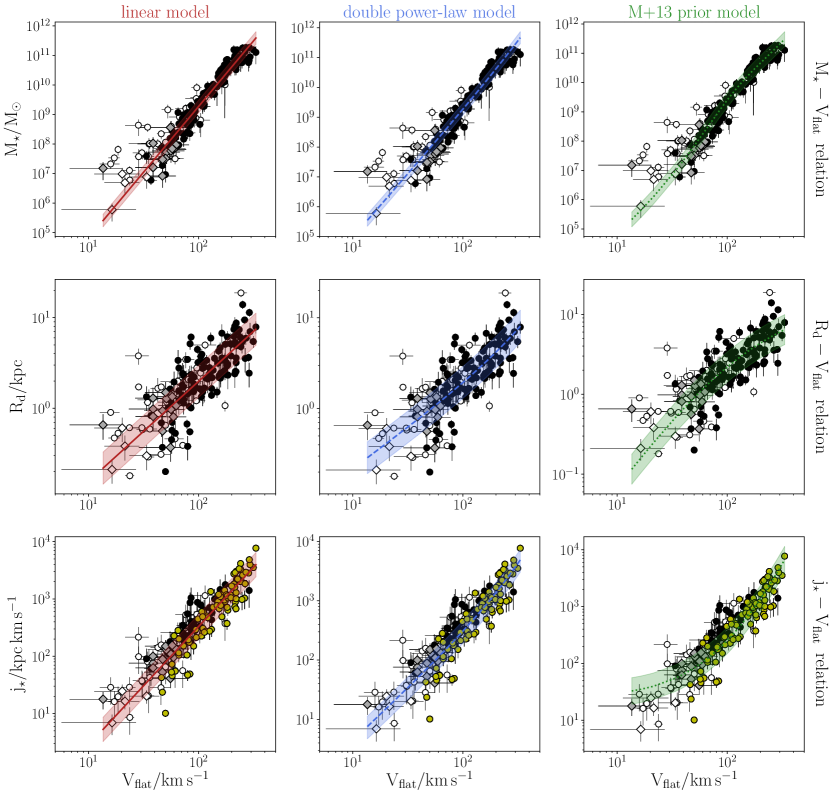
Figure 2: Comparison of the three best models obtained with different assumptions on $f_{j}$, $f_{M}$, and $f_{V}$ with the data from SPARC galaxies (circles) and LITTLE THINGS galaxies (diamonds). Each column shows the fits for a given model, following the assumptions in Sec. 3.3. The top row is for the stellar Tully-Fisher relation, the middle row is for the size-velocity relation, while the bottom row is for the angular momentum-velocity relation. The white filled points in the plots are the galaxies which do not satisfy the Lelli et al. (2016b) criterion on the flatness of their rotation curves. The yellow filled points in the $j_{\star}-V_{\rm flat}$ relation are the 92 SPARC galaxies with ‘onverged $j_{\star}$ profiles, following Posti et al. (2018a).

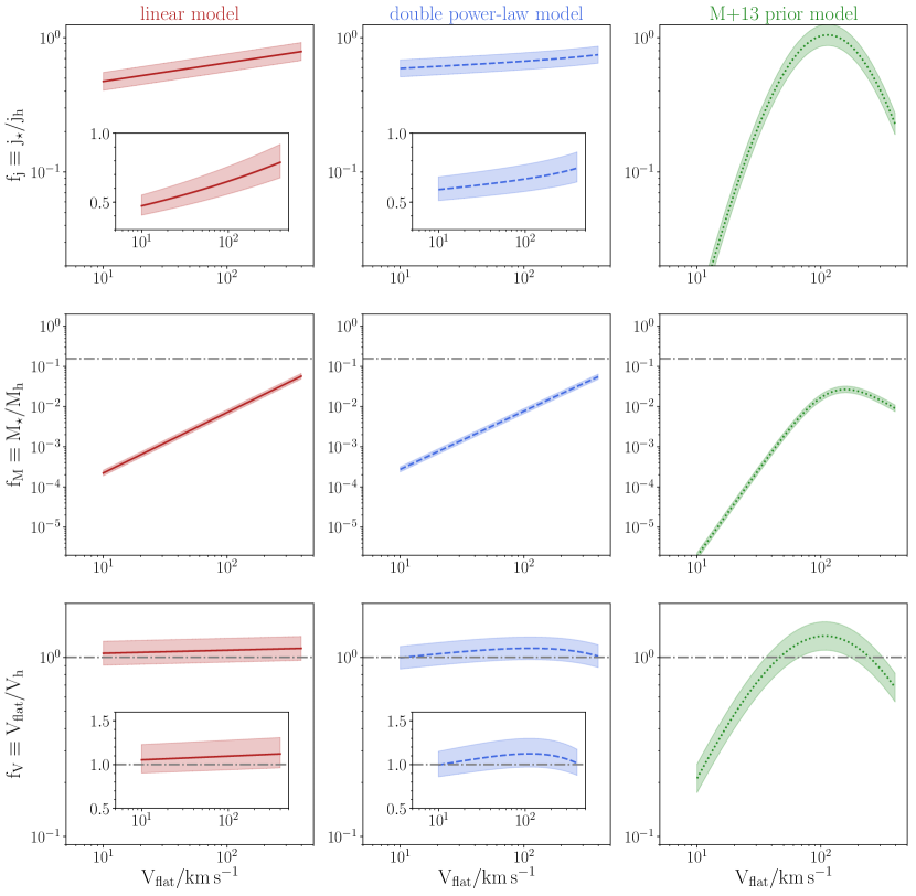
Figure 3: Model predictions. We show how $f_{j}$ (top row), $f_{M}$ (middle row), and $f_{V}$ (bottom rows) vary as a function of $V_{\rm flat}$ for the three best models (columns). In the middle row the dot-dashed line shows the value of the cosmic baryon fraction $f_{\rm b}=0.157$, while in the bottom row the dot-dashed line indicates the value $f_{V}=1$. The insets show a zoom-in of the plots in linear scale.

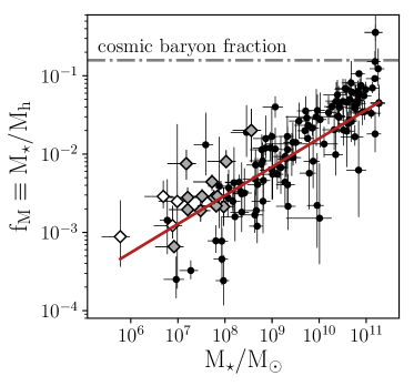
Figure 4: Global star formation efficiency $f_{M}\equiv M_{\star}/M_{\rm h}$ as a function of $M_{\star}$ for the SPARC and LITTLE THINGS galaxies. The measurements of the halo masses come from PFM19 and Read et al. (2017), respectively. Symbols are the same as in Fig. 2. The red line indicates the $f_{M}-M_{\star}$ relation derived in the linear model for guidance.

Figure 5: Comparison of the predictions of the three models in the $V_{\rm flat}-V_{\rm h}$ plane, with data for the SPARC (circles) and LITTLE THINGS galaxies (diamonds). The halo virial velocities have been obtained with a careful rotation curve decomposition by Read et al. (2017) for the LITTLE THINGS galaxies and by PFM19 for the SPARC galaxies. In all panels, the grey dot-dashed line is the 1:1 and the symbols are the same as in Fig. 2.

4.2 Three fundamental fractions from dwarfs to massive spirals

In Figure 3 we show the predictions of the three best models (on each column) of the three fundamental fractions, respectively $f_{j}$, $f_{M}$, and $f_{V}$, as a function of $V_{\rm flat}$ (on each row). The most important and most striking result to notice is that the predictions of the three fractions behave similarly in the linear and double power-law models. For the vast majority of galaxies the predictions of these two models, which are by far statistically preferred to the M+13 prior model, are in remarkable agreement, considering that they have very different functional forms and degrees of freedom. The fact that the agreement is so detailed in $f_{M}$, $f_{j}$, and $f_{V}$ ensures that the result is robust and confirms that the data have enough information to infer these fractions. This can, thus, be regarded as a major success of the modelling approach presented in this work.

Along the same lines, another interesting result is that even when allowing the behaviour of the three fractions to change slope at a characteristic velocity ($\log\,V_{0}$), i.e. the parameters preferred by the data, $f_{M}$ and $f_{V}$ do not have a significant break at the scale of Milky Way-sized galaxies. This is a key prediction of abundance matching models. Considering that the best M+13 prior model which breaks at $V_{0}\approx 125$ km/s is statistically disfavoured, we conclude that the observed scaling laws of nearby discs do not provide clear indications of any break in the behaviour of the fundamental fractions at the scale of $L^{\ast}$ galaxies (e.g. McGaugh et al. 2010).

Both the best linear and double power-law models have a global star formation efficiency which grows monotonically with galaxy mass, approximately as $M_{\star}^{1/3}$. Henceforth, the most efficient galaxies at forming stars are the most massive spirals ($M_{\star}\gtrsim 10^{11}M_{\odot}$, $V_{\rm flat}\gtrsim 250$ km/s), qualitatively confirming previous results on detailed rotation curve decomposition ( PFM19, see Sec. 4.3 for a more in-depth comparison). We also note that the most massive spirals in both models have $f_{M}\sim f_{\rm b}$, which implies that these systems have virtually no missing baryons (PFM19).

The retained fraction of angular momentum is, on the other hand, remarkably constant ($f_{j}\approx 0.6$) over the entire range probed by our galaxy sample ($\sim$1.5 dex in velocity, $\sim$5 dex in mass). Putting together our two main findings on $f_{M}$ and $f_{j}$, we are now able to cast new light on why disc galaxies today have comparable angular momenta to those of their dark haloes. Since the slopes of the power-law $j-M$ relations for galaxies and haloes are nearly the same within the uncertainties ($\sim 2/3$), then from $j_{\star}\propto f_{j}f_{M}^{-2/3}M_{\star}^{2/3}$ it follows that the factor $f_{j}f_{M}^{-2/3}$ has to be nearly constant with mass (e.g. Romanowsky & Fall 2012, their Eq.s 15-16). This implies that the retained fraction of angular momentum has to correlate with the global star formation efficiency ($\log f_{j}\propto\log f_{M}$) to reproduce the observed scalings. Most of the earlier investigations on $f_{j}$ found that it was nearly constant with mass (Dutton & van den Bosch 2012; Romanowsky & Fall 2012; Fall & Romanowsky 2013, 2018), since they all adopted a monotonic $f_{M}$ (from Dutton et al. 2010). Posti et al. (2018b), instead, used different models for the stellar-to-halo mass relation to derive $f_{j}$ as a function of mass such that the observed Fall relation was reproduced. Since most of the contemporary and popular models for $f_{M}=f_{M}(M_{\star})$ have a bell shape, the constraint $\log f_{j}\propto\log f_{M}$ led these authors to conclude that a bell-shaped $f_{j}=f_{j}(M_{\star})$ was also favoured. This, in turn, implies for instance that dwarfs should have significantly smaller $f_{j}$ than $L^{\ast}$ galaxies (e.g. El-Badry et al. 2018; Marshall et al. 2019). However, the recent halo mass estimates by PFM19 indicated that spirals are following a simpler stellar-to-halo mass relation, roughly $f_{M}\propto M_{\star}^{1/3}$. This, together with the constraint $f_{j}f_{M}^{-2/3}\approx const.$ implies a very weak dependence of $f_{j}$ on stellar mass, roughly $f_{j}\propto M_{\star}^{2/9}$. The comprehensive analysis presented in this paper confirms this and points towards an even weaker dependence of $f_{j}$ on mass, which is consistent with this value being constant ($f_{j}\approx 0.6$) within the scatter.

The velocity fraction $f_{V}$ is found to be always compatible with unity in the linear and double power-law models. The expression $f_{V}\approx 1$ means that discs are rotating close to the halo virial velocity, which roughly matches what is seen in hydrodynamical simulations at the high-mass end (e.g. Ferrero et al. 2017); this is also supported by any reasonable mass decomposition (e.g. PFM19, ). Similar to the case of $f_{j}$, $f_{V}$ also turns out to depend substantially on $f_{M}$. If $f_{M}$ is monotonic then $f_{V}$ is also monotonic and close to unity; while, if $f_{M}$ has a non-monotonic bell shape, then $f_{V}$ also follows a similar behaviour, rapidly plunging below unity for both dwarfs and high-mass spirals. Considering a Tully-Fisher relation of the type $V_{\rm flat}\propto M_{\star}^{\delta}$ and writing $V_{\rm flat}\propto f_{V}f_{M}^{-1/3}M_{\star}^{1/3}$ (see e.g. Appendix B), then it follows that $f_{V}\propto f_{M}^{1/3}M_{\star}^{\delta-1/3}$, which means that roughly $f_{V}\propto f_{M}^{1/3}$ since the extra dependence on $M_{\star}$ is very weak ($\delta\simeq 0.25-0.3$). The implication of this is that if $f_{M}$ has a bell shape as expected from abundance matching models, then also $f_{V}$ will have a similar shape (e.g. Cattaneo et al. 2014; Ferrero et al. 2017). With our comprehensive analysis we find that such models are statistically disfavoured by the data, which instead favour a monotonically increasing $f_{M}$ and a roughly constant $f_{V}\approx 1$. We can now conclude that our results provide a simple and appealing explanation to why the observed scaling laws are single, unbroken power laws: the galaxy–halo connection is linear and the fractions (6) are single-slope functions of velocity (or mass), instead of being complicated non-monotonic functions which, when combined as in Eqs. (8)-(10), conspire to yield power-law scaling relations.

To make sure that these results are not valid only for the SPARC+LITTLE THINGS sample we considered, we repeated the same analysis on the much larger galaxy sample from Courteau et al. (2007). This sample contains about 1300 spiral galaxies found in different environments and it has a higher completeness than SPARC. However, the mass range is more limited ($8\lesssim\log M_{\star}/M_{\odot}\lesssim 11.7$) and the data quality is poorer, since it relies on optical (H$\alpha$) rotation curves, the disc scale lengths are typically more uncertain and we have to use estimator (2) to compute $j_{\star}$ for all galaxies. Nevertheless, when we built the three scaling relations and we fitted the three models, we arrived at basically the same main conclusions as above: the linear and double power-law models have very similar predictions for $f_{j}$, $f_{M}$, and $f_{V}$ and they are statistically preferred to the M+13 prior model. Thus, from this test we conclude that the results we inferred on the fundamental fractions using the SPARC+LITTLE THINGS sample are generally applicable for all regularly rotating disc galaxies.

Finally, we note that assuming a linear or double power-law functional form for the behaviour of the three fractions as a function of $V_{\rm flat}$ does not bias our results. We tested this by fitting a non-parametric model, where we do not assume any functional form for the behaviour of $f_{j}$, $f_{M}$, and $f_{V}$ as a function of $V_{\rm flat}$. Instead, we bin the range in $V_{\rm flat}$ spanned by the data with five bins of different sizes, such that the number of galaxies per bin is roughly equal. We, thus, constrained the five values of $f_{j}$, $f_{M}$, and $f_{V}$, together with the intrinsic scatter $\sigma_{\log\,f}$, for a grand total of 16 degrees of freedom. The resulting predictions on the three fractions are very well compatible with those of the linear or double power-law models; we show these predictions in Appendix C.

4.3 Comparison of the predicted $f_{M}$ with detailed rotation curve decomposition

The three best models that we fitted to the stellar Tully-Fisher, size-mass, and Fall relations, directly predict the virial masses of the dark matter haloes hosting these spirals. Luckily all these galaxies have good enough photometric and kinematic data to allow for an accurate decomposition of their observed HI rotation curve, which can be used to get a robust measurement of their halo masses. In particular, PFM19 and Read et al. (2017) have carefully performed fits to the observed rotation curves for the SPARC and LITTLE THINGS samples, respectively, and have provided measurements of $V_{\rm h}$. We show in Figure 4 the measurements of $f_{M}$ for these galaxies. Since these measurements rely on fits of the dark matter halo profile and since they have not been used in the model fit carried out in this paper, we can now check a posteriori if the predictions of our three best models agree with the global shape of the halo profile inferred from the HI rotation curves.

We show this comparison in Figure 5, in which we plot the observed $V_{\rm flat}$ against the $V_{\rm h}$ measured from the rotation curve decomposition; predictions from the three best models are superimposed. The predictions of the linear model are by far in best agreement with the measurements.

The double power law is in a similar remarkable agreement for all galaxies. From this check we conclude that these two models both provide a good description of the observed disc galaxy population, but with a preference for the linear model from a statistical point of view, i.e. from the standard statistical criteria AIC and BIC. On the other hand, the M+13 prior model manifestly fails at reproducing the measured distribution of galaxies in the $V_{\rm flat}-V_{\rm h}$ plane, both at low masses and, possibly, at high masses. According to the predictions of this model, both dwarfs and very massive spirals should inhabit much more massive dark matter haloes than what it is suggested from their HI rotation curves. This has already been noted and dubbed the “too big to fail” problem in the field (Papastergis et al. 2015).

Thus, we conclude that a simple empirical model (of the type Eqs. 8-10), in which all disc galaxies follow a stellar-to-halo mass relation which has a peak at $M_{\star}\sim 3\times 10^{10}M_{\odot}$, predicts galaxy formation fundamental parameters that are discrepant with measurements of the kinematics of cold gas in spirals. A simple tight and linear galaxy–halo connection, in disagreement with abundance matching, however fully cures this too big to fail problem.

5 Conclusions

In this paper we used the observed stellar Tully-Fisher, size-mass, and Fall relations of a sample of $\sim 150$ nearby disc galaxies, from dwarfs to massive spirals, to empirically derive three fundamental parameters of galaxy formation: the global star formation efficiency ($f_{M}$), the retained fraction of angular momentum ($f_{j}$), and the ratio of the asymptotic rotation velocity to the halo virial velocity ($f_{V}$).

Under the usual assumption that the galaxy size is related to its specific angular momentum, we used an analytic model to predict the distribution of discs in the mass-velocity, size-velocity, and angular momentum-velocity planes. We defined three models with different parametrisations of how the three fundamental parameters vary as a function of asymptotic velocity (or galaxy mass): we thus tested a linear model, a double power-law model, and another with a double power-law behaviour, but with prior imposed such that the model follows the expectations from widely used abundance matching stellar-to-halo mass relations for the global star formation efficiency (the M+13 prior model).

We find the best-fitting parameters in each of these models and their posterior probabilities performing a Bayesian analysis. We briefly summarise our main findings:

• We find reasonably good fits of the observed scaling relations in all three cases that we have tested.

• By assuming that the intrinsic scatter is the same for all three fundamental fractions (for computational simplicity), we find that this scatter has to be particularly small ($\sigma_{\log\,f}\simeq 0.07\pm 0.01$ dex) to account for the intrinsic scatters of the three observed scaling relations.

• We determined that the statistically preferred model is that where the fundamental galaxy formation parameters vary linearly with galaxy velocity (or mass) using standard statistical criteria (AIC & BIC). On the other hand, the model with standard abundance matching priors (from M+13, ) is largely disfavoured by the data. We conclude that models where the galaxy–halo connection is complex and non-monotonic statistically provide an overfit to the structural scaling relations of discs.

• We empirically derive and show how the three fundamental parameters vary as a function of galaxy rotation velocity. We find that in the best-fitting linear and double power-law models the three fractions have a remarkable similar behaviour, despite having completely different functional forms. This ensures that the observed scaling laws really provide a strong, data-driven inference on the galaxy–halo connection.

• We confirm previous indications that the retained fraction of angular momentum and the ratio of the asymptotic-to-virial velocity strongly depend on the global star formation efficiency (e.g. Navarro & Steinmetz 2000; Cattaneo et al. 2014; Posti et al. 2018b); in particular, they are non-monotonic only if the latter is non-monotonic.

• In the statistically preferred models, the retained fraction of angular momentum is relatively constant across the entire mass range ($f_{j}\sim 0.6$) as is the ratio of the asymptotic-to-virial velocity ($f_{V}\sim 1$). On the other hand, the global star formation efficiency is found to be a monotonically increasing function of mass, implying that the most efficient galaxies at forming stars are the most massive spirals (with $f_{M}\sim f_{\rm b}$), whose star formation efficiency has not been quenched by strong feedback (the failed feedback problem).

• Finally, we compared a posteriori the predictions of the three models with the dark matter halo masses found by Read et al. (2017) and PFM19 from the detailed analysis of rotation curves in the LITTLE THINGS and SPARC galaxy samples. We found that the M+13 prior model is strongly rejected since it significantly overpredicts the halo masses especially at low $V_{\rm flat}$, but also at high $V_{\rm flat}$. This too big to fail problem (Papastergis et al. 2015) is fully solved in the linear model, which best describes the measurements.

Our analysis leads us to conclude that the statistically favoured explanation to why the observed scaling laws of discs are single, unbroken power laws is the simplest possible: the fundamental galaxy formation parameters for spiral galaxies are tight single-slope monotonic functions of mass, instead of being complicated non-monotonic functions.

The present study and the associated failed feedback problem concern only disc galaxies. It is known that when including also spheroids, which dominate the galaxy population at the high-mass end, the inferred galaxy-halo connection becomes highly non-linear. In particular, it appears that there is a clear difference in the stellar-to-halo mass relations for spirals and ellipticals at least at the high-mass end, as probed statistically using many observables (e.g. Conroy et al. 2007; Dutton et al. 2010; More et al. 2011; Wojtak & Mamon 2013; Mandelbaum et al. 2016; Lapi et al. 2018). Thus, the results found in this work and those of PFM19 could in principle be reconciled with conventional abundance matching if the galaxy-halo connection is made dependent on galaxy type. This can be achieved for instance if discs and spheroids have significantly different formation pathways, i.e. in accretion history, environment etc., which are still encoded today in their different structural properties (e.g. also Tortora et al. 2019). Whether this is the case in current simulations of galaxy formation, and whether the failed feedback problem in massive discs can be addressed within those simulations is the next big question to be asked.

The model preferred by the SPARC and LITTLE THINGS data has a monotonic $f_{M}$ approximately proportional to $M_{\star}^{1/3}$. With this global star formation efficiency, it turns out that the retained fraction of angular momentum $f_{j}$ needs to be high and relatively constant for discs of all mass ($f_{j}\approx 0.5-0.9$). This is because the observed Fall relation has a similar slope to the specific angular momentum-mass relation of dark matter haloes: since $f_{j}\approx const$, a simple correspondence $j_{\star}\propto j_{\rm h}$ is in remarkable agreement with the observations (Romanowsky & Fall 2012; Posti et al. 2018b). This implies that the current measurements are compatible with a model in which discs have overall retained about all the angular momentum that they gained initially from tidal torques. This is to be intended in an integrated sense in the entire galaxy: it can not simply have happened with every gas element having conserved their angular momentum (sometimes referred to as “detailed” or “strong” angular momentum conservation) because dark matter haloes and discs have completely different angular momentum distributions today (Bullock et al. 2001; van den Bosch et al. 2001). Thus, even if stars and dark matter appear to have a simple correspondence $j_{\star}\propto j_{\rm h}$, it remains unclear and unexplained how the angular momentum of gas and stars has redistributed during galaxy formation and why the total galaxy’s specific angular momentum is still proportional to that of its halo.

Some disc galaxies, especially dwarfs, have huge cold gas reservoirs which sometimes dominate over their stellar budget. These systems are typically outliers of the (stellar) Tully-Fisher, but they instead lie on the baryonic Tully-Fisher relation, which is obtained by replacing the stellar mass with the baryonic mass ($M_{\rm baryons}=M_{\star}+M_{\rm HI}$, see e.g. McGaugh et al. 2000; Verheijen 2001). More galaxies adhere to this relation, which is also tighter than the stellar Tully-Fisher, suggesting that it is a more fundamental law (e.g. Lelli et al. 2016b; Ponomareva et al. 2018). Thus, considering baryonic fractions instead of stellar fractions (Eq. 6) in a model such as that of Sec. 3 would presumably give us deeper and more fundamental insight into how baryons cooled and formed galaxies. To do this, it is thus imperative to have a baryonic counterpart of the size-mass and Fall relations (e.g. Obreschkow & Glazebrook 2014; Kurapati et al. 2018), for a sample of spirals sufficiently large in mass. We plan to report on the latter soon, establishing first whether the observed baryonic Fall relation is tighter and more fundamental than the stellar Fall relation.

Appendix A Size and angular momentum fractions in disc galaxies

The specific angular momentum of an exponential disc with a flat rotation curve $V_{\rm flat}=f_{V}V_{\rm h}$ is

$$j_{\star}=\frac{\int{\rm d}R\,R^{2}\,\exp\left(-R/R_{\rm d}\right)\,V_{\rm flat}}{\int{\rm d}R\,R\,\exp\left(-R/R_{\rm d}\right)}=2R_{\rm d}f_{V}V_{\rm h}.$$ (21)

From Eqs. (4)-(5) and introducing $f_{j}$ and $f_{R}$ as in Eq. (6), we have

$$R_{\rm d}=\frac{f_{R}}{H}\sqrt{\frac{2}{\Delta}}V_{\rm h};$$ (22)

$$j_{\star}=\frac{2\lambda f_{j}}{H\sqrt{\Delta}}V_{\rm h}^{2}.$$ (23)

Plugging Eq. 21 into Eq. 23 we obtain

$$R_{\rm d}=\frac{f_{j}\lambda}{f_{V}H\sqrt{\Delta}}V_{\rm h},$$ (24)

which, using Eq. 22, can be rearranged as

$$f_{R}=\frac{\lambda}{\sqrt{2}}\frac{f_{j}}{f_{V}}.$$ (25)

A very similar relation to this was already derived by Fall & Efstathiou (1980) and Mo et al. (1998), who started by assuming that $j_{\star}=2R_{\rm d}V_{\rm h}$ to replace Eq. (21) and got $f_{R}=\lambda f_{j}/\sqrt{2}$. In this work we are interested in deriving simultaneous constraints on $f_{j}$,$f_{M}$, and $f_{V}$, thus we prefer to use the formulation in Eq. (25), which allows the flat asymptotic circular velocity $V_{\rm flat}$ to differ from the halo virial velocity $V_{\rm h}$. We have, however, checked that using $f_{R}=\lambda f_{j}/\sqrt{2}$ instead of Eq. (25) does not significantly alter the fits of the models.

Appendix B Fitting $f_{j}$, $f_{M}$, and $f_{V}$ as a function of $M_{\star}$

In this Appendix we demonstrate that considering $M_{\star}$ as the independent observable, and thus fitting the canonical Tully-Fisher, size-mass, and Fall relations, yields similar predictions for the fractions $f_{j}$, $f_{M}$, and $f_{V}$ to what we obtained above.

We start from the equations for dark matter, i.e.

$$V_{\rm h}=\left(\sqrt{\frac{\Delta}{2}}GHM_{\rm h}\right)^{1/3};$$ (26)

$$R_{\rm h}=\left(\frac{2GM_{\rm h}}{\Delta H^{2}}\right)^{1/3};$$ (27)

$$j_{\rm h}=\frac{\lambda}{(\Delta H^{2})^{1/6}}\left(2GM_{\rm h}\right)^{2/3}.$$ (28)

After introducing the three fractions, we have

$$V_{\rm flat}=f_{V}\left(\sqrt{\frac{\Delta}{2}}\frac{GHM_{\star}}{f_{M}}\right)^{1/3};$$ (29)

$$R_{\rm d}=\frac{\lambda f_{j}}{f_{V}}\left(\frac{GM_{\star}}{\sqrt{2}\Delta H^{2}f_{M}}\right)^{1/3};$$ (30)

$$j_{\star}=\frac{\lambda f_{j}}{(\Delta H^{2})^{1/6}}\left(\frac{2GM_{\star}}{f_{M}}\right)^{2/3}.$$ (31)

The three equations above are used to fit the observations in the $V_{\rm flat}-M_{\star}$, $R_{\rm d}-M_{\star}$ and $j_{\star}-M_{\star}$ diagrams.

Similar to Sec. 3.3, we try three different models as follows:

• the linear model, where

  $$\log\,f=\alpha\log M_{\star}/M_{\odot}+\log\,f_{0}.$$ (32)

• the double power-law model, where

  $$f=f_{0}\left(\frac{M_{\star}}{M_{0}}\right)^{\alpha}\left(1+\frac{M_{\star}}{M_{0}}\right)^{\beta-\alpha}.$$ (33)

• the M+13 prior” model, which is the same as case (ii), but with priors on $f_{M}$ from the abundance matching model of M+13.

We show in Figure 6-7, which are analogous to Fig. 2-3, the data/model comparisons and the constraints on the fundamental fractions, respectively. The behaviour of the models is largely identical to those in the main text; the only noticeable difference is that the double power-law model now has a slight break at low masses (at $\sim 10^{6}M_{\odot}$). However the statistical significance of this break is very low since it is driven by just a few data points in the dwarf regime, where the uncertainties are higher. On the other hand, for this model we still find no indications of a break at around $L^{\ast}$ galaxies. Finally, we note that also in this case we find that the statistically preferred model is the linear model, according to the AIC & BIC criteria: $(\Delta{\rm AIC},\Delta{\rm BIC})=(1.4,13.3)$ with respect to the double power-law model and $(\Delta{\rm AIC},\Delta{\rm BIC})=(28.2,40.1)$ with respect to the M+13 prior model.

Table 3: Posterior distributions for the three models with $M_{\star}$ as the main independent observable quantity. This Table is analogous to Tab. 1 and the models and the equations fitted described in App. B.

	linear	double power law	M+13 prior
$\log\,f_{0,j}$	$-0.36^{+0.57}_{-0.57}$	$-0.33^{+0.34}_{-0.37}$	$0.33^{+0.07}_{-0.06}$
$\log\,M_{0}/M_{\odot}$	–	$3.6^{+0.6}_{-0.4}$	$10.76^{+0.04}_{-0.05}$
$\alpha_{j}$	$0.02^{+0.06}_{-0.06}$	$2^{+25}_{-26}$	$0.25^{+0.04}_{-0.04}$
$\beta_{j}$	–	$0.04^{+0.06}_{-0.06}$	$-1.9^{+0.15}_{-0.15}$
$\log\,f_{0,M}$	$-5.3^{+0.7}_{-0.7}$	$-4.1^{+0.4}_{-0.5}$	$-1.1^{+0.05}_{-0.05}$
$\alpha_{M}$	$0.35^{+0.07}_{-0.07}$	$3^{+25}_{-27}$	$0.61^{+0.04}_{-0.04}$
$\beta_{M}$	–	$0.4^{+0.07}_{-0.07}$	$1.63^{+0.05}_{-0.05}$
$\log\,f_{0,V}$	$0.11^{+0.24}_{-0.24}$	$0.06^{+0.14}_{-0.15}$	$0.26^{+0.03}_{-0.03}$
$\alpha_{V}$	$0.01^{+0.02}_{-0.02}$	$-11^{+25}_{-19}$	$0.1^{+0.02}_{-0.02}$
$\beta_{V}$	–	$0.01^{+0.02}_{-0.02}$	$-0.87^{+0.07}_{-0.07}$
$\sigma_{\log\,f}$	$0.07^{+0.01}_{-0.01}$	$0.07^{+0.01}_{-0.01}$	$0.08^{+0.01}_{-0.01}$

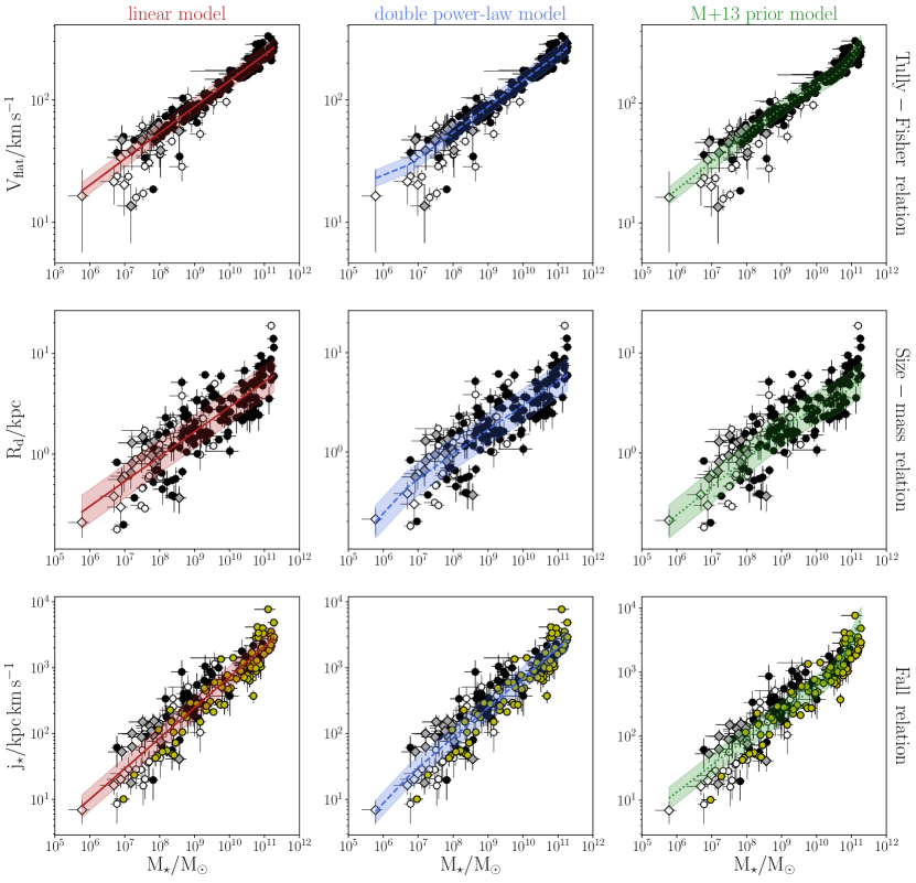
Figure 6: Comparison of the three models described in Appendix B with the data on the Tully-Fisher, size-mass, and Fall diagrams. Curves and symbols are analogous to Fig. 2.

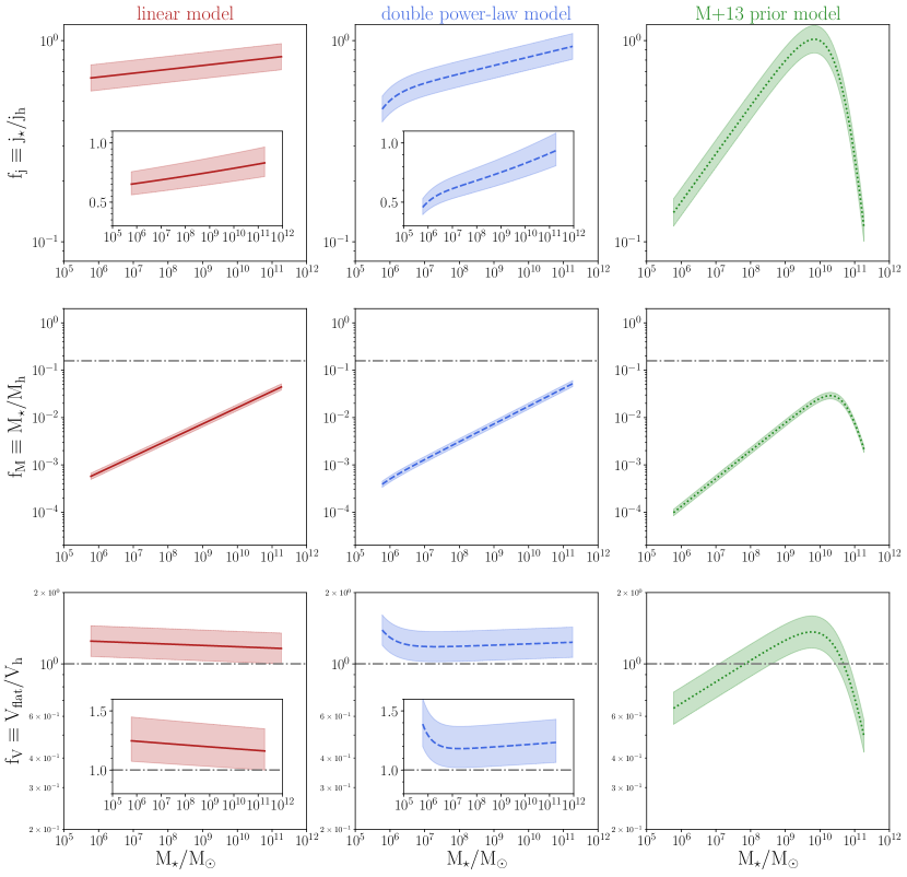
Figure 7: Behaviour of the three fractions as a function of $M_{\star}$ in the three models of Appendix B. Curves and symbols are analogous to Fig. 3.

Appendix C Non-parametric model

In this Appendix, we describe a model in which the variation of $f_{j}$, $f_{M}$, and $f_{V}$ as a function of $V_{\rm flat}$ has a completely free form. This model is aimed to test whether the functional forms that we have chosen in Sec. 3.3 are too restrictive for the data that we considered, and if the data themselves are informative enough to constrain a different behaviour.

We binned the range in $V_{\rm flat}$ spanned by the data, [15,320] km/s, into five bins of different sizes, such that the number of galaxies in each bin is roughly equal. We, then, constrained the five (constant) values of $f_{j}$, $f_{M}$, and $f_{V}$ in each bin maximising the same likelihood as in Sec. 3.5. Together with the intrinsic scatter $\sigma_{\log\,f}$, this model has a total of 16 degrees of freedom.

Figure 8 shows the three fractions in this model as a function of $V_{\rm flat}$. A part from a small difference in the lowest $V_{\rm flat}$ bin, where dwarf galaxies with the highest uncertainties dominate, the predictions of this model are in remarkable agreement with those of the linear and double power-law models. Also the intrinsic scatter that we fit with this model is very well comparable with that of the other cases, where $\sigma_{\log\,f}=0.08\pm 0.05$. This ensures that the linear or double power-law functional forms that we adopted for our fiducial models are not too restrictive for the data that we have at hand.

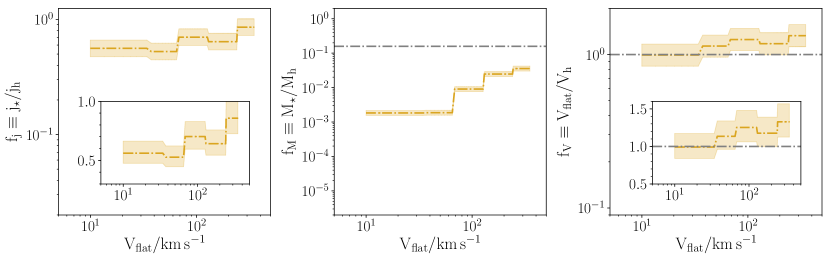
Figure 8: Fundamental fractions as a function of the asymptotic rotation velocity for the non-parametric model (gold dot-dashed lines, with the band encompassing the intrinsic scatter $\sigma_{\log\,f}$). The three fractions are binned in 5 bins in $V_{\rm flat}$ (with roughly the same number of galaxies). The panels are in the same scale as those in Fig. 3.