High order discretization methods for spatial-dependent epidemic models

Abstract

In this paper, an epidemic model with spatial dependence is studied and results regarding its stability and numerical approximation are presented. We consider a generalization of the original Kermack and McKendrick model in which the size of the populations differs in space. The use of local spatial dependence yields a system of partial-differential equations with integral terms. The uniqueness and qualitative properties of the continuous model are analyzed. Furthermore, different spatial and temporal discretizations are employed, and step-size restrictions for the discrete model’s positivity, monotonicity preservation, and population conservation are investigated. We provide sufficient conditions under which high-order numerical schemes preserve the stability of the computational process and provide sufficiently accurate numerical approximations. Computational experiments verify the convergence and accuracy of the numerical methods.

1 Introduction

During the course of human history, many epidemics have ravaged the population. Since the plague of Athens in 430 BC described by historian Thucydides (one of the earliest descriptions of such epidemics), researchers tried to model and explain the outbreak of illnesses. More recently, the outbreak of the COVID-19 pandemic revealed the importance of epidemic research and the development of models to describe the public health impact of major virus diseases.

Nowadays, many of the models used in science are derived from the original ideas of Kermack and McKendrick [Kermack/McKendrick:1927:MathematicalEpidemics] in 1927, who constructed a compartment model to study the process of epidemic propagation. In their model, usually referred to as the SIR model, the population is split into three classes: $S$ being the group of healthy individuals who are susceptible to infection; $I$ is the compartment of the ill species who can infect other individuals; and $R$ being the class of recovered or immune individuals. The original model of Kermack and McKendrick took into account constant rates of change and neglected any natural deaths and births or vaccination. In this work, we also consider constant rates of change, and in addition, we include the term $c\,S(t)$ to describe immunization effects through vaccination. The SIR model takes the form

$$\left\{\begin{aligned} \frac{d}{dt}S(t)&=-a\,S(t)I(t)-c\,S(t),\\ \frac{d}{dt}I(t)&=a\,S(t)I(t)-b\,I(t),\\ \frac{d}{dt}R(t)&=b\,I(t)+c\,S(t),\end{aligned}\right.$$ (1.1)

where the positive constant parameters $a$, $b$ and $c$ correspond to the rate of infection, recovery and vaccination, respectively.

Since the introduction of the model (1.1) in 1927, numerous extensions were constructed to describe biological processes more efficiently and realistically. A natural extension is to take into account the heterogeneity of the domain so that we examine not only the change of the populations in time but also observe the spatial movements. Kendall introduced such models that transformed the system of ordinary differential equations (1.1) into a system of partial differential equations [Bartlett:1957:MeaslesPeriodicity, Kendall:1965:ModelsInfection].

The time-dependent functions in (1.1) represent the number of individuals in each class but contain no information about their spatial distribution. Instead, one can replace these concentration functions with spatial-dependent functions describing the density of healthy, infectious, and recovered species over some domain $\Omega\subset\mathbb{R}^{d}$ [Takacs/Horvath/Farago:2019:SpaceModelsDiseases]. In this paper, we consider a bounded domain in $\mathbb{R}^{2}$; hence the system (1.1) is recast as

$$\left\{\begin{aligned} \frac{\partial}{\partial t}S(t,x,y)&=-a\,S(t,x,y)I(t,x,y)-c\,S(t,x,y),\\ \frac{\partial}{\partial t}I(t,x,y)&=a\,S(t,x,y)I(t,x,y)-b\,I(t,x,y),\\ \frac{\partial}{\partial t}R(t,x,y)&=b\,I(t,x,y)+c\,S(t,x,y).\end{aligned}\right.$$ (1.2)

However, the model (1.2) is still insufficient as it does not allow the disease to spread in the domain but only accounts for a point-wise infection. Spatial points do not interact with each other but infect species only at their location. To allow a realistic propagation of the infection, we assume that an infected individual can spread the disease on susceptible species in a certain area around its location. Let us define a non-negative function with compact support

$$G(x,y,r,\theta)=\begin{cases}g_{1}(r)g_{2}(\theta,x,y),&\text{if }\bigl{(}\bar{x}(r,\theta),\bar{y}(r,\theta)\bigr{)}\in B_{\delta}(x,y),\\ 0,&\text{otherwise,}\end{cases}$$ (1.3)

that describes the effect of a single point $(x,y)$ in a $\delta$-radius neighborhood $B_{\delta}(x,y)$, and set $\bar{x}(r,\theta)=x+r\cos(\theta)$ and $\bar{y}(r,\theta)=y+r\sin(\theta)$. The function $G(x,y,r,\theta)$ demonstrates how healthy individuals at points $(\bar{x}(r,\theta),\bar{y}(r,\theta))$ are infected by the center point $(x,y)$, where $r\in[0,\delta]$ is the distance from the center and $\theta\in[0,2\pi)$ is the angle. In this work we consider $G(x,y,r,\theta)$ to be a separable function. The effect the center point $(x,y)$ has at a distance $r$ is described by $g_{1}(r)$; a decreasing, non-negative function that is equal to zero for values $r\geq\delta$ (since there is no effect outside $B_{\delta}(x,y)$). The function $g_{2}(\theta,x,y)$ characterizes the angular effect, i.e., the effect at an angle $\theta$ with respect to the center point $(x,y)$. The case of a spatially independent function $g_{2}(\theta,x,y)$, that is the same for all $(x,y)\in\Omega$, is widely studied in [Farago/Horvath:2016:SpaceTimeEpidemic] and [Farago/Horvath:2018:QualitativeDiseasePropagation]. A more generic function the depends on spatial coordinates could be useful in the case of epidemic diseases with a given direction of propagation, or in the case of wildfires when the wind profile is known. Such a function with a constant wind direction was described in [Takacs/Horvath/Farago:2019:SpaceModelsDiseases]. In both cases it is supposed that $g_{2}$ is bounded and periodic in the sense that $g_{2}(0,x,y)=\lim_{\theta\rightarrow 2\pi}g_{2}(\theta,x,y)$, for each $(x,y)\in\Omega$.

The nonlinear terms of the right-hand side of (1.2) describe the interaction of susceptible and infected species. We can now utilize (1.3) and replace the density of infected species in these nonlinear terms by

$$\int_{0}^{\delta}\int_{0}^{2\pi}G(x,y,r,\theta)I\bigl{(}t,\bar{x}(r,\theta),\bar{y}(r,\theta)\bigr{)}\,r\,\mathrm{d}\theta\,\mathrm{d}r,$$

where we used the fact that $G(x,y,r,\theta)=0$ outside the ball $B_{\delta}(x,y)$. Therefore, the model (1.2) can be extended as a system of integro-differential equations

$$\left\{\begin{aligned} \frac{\partial S(t,x,y)}{\partial t}&=-S(t,x,y)\int_{0}^{\delta}\int_{0}^{2\pi}g_{1}(r)g_{2}(\theta,x,y)I\bigl{(}t,\bar{x}(r,\theta),\bar{y}(r,\theta)\bigr{)}\,r\,\mathrm{d}\theta\,\mathrm{d}r-cS(t,x,y),\\ \frac{\partial I(t,x,y)}{\partial t}&=S(t,x,y)\int_{0}^{\delta}\int_{0}^{2\pi}g_{1}(r)g_{2}(\theta,x,y)I\bigl{(}t,\bar{x}(r,\theta),\bar{y}(r,\theta)\bigr{)}\,r\,\mathrm{d}\theta\,\mathrm{d}r-bI(t,x,y),\\ \frac{\partial R(t,x,y)}{\partial t}&=bI(t,x,y)+cS(t,x,y).\end{aligned}\right.$$ (1.4)

We consider homogeneous Dirichlet conditions since we assume that there is no susceptible population outside of the domain $\Omega$, and there is no diffusion in (1.4).

1.1 Outline and scope of the paper

The aim of this paper is twofold. First, in section 2sec:Analyticalsec:Analytical we analyze the stability of the continuous model (1.4) and prove that a unique solution exists under some Lipschitz continuity and boundedness assumptions. Secondly, in sections 3 and 4sec:Spatialsec:Spatialsec:TimeIntegrationsec:TimeIntegration we seek numerical schemes that approximate the solution of (1.4) and maintain its qualitative properties.

We verify that the analytic solution satisfies biologically reasonable properties; however, as shown in section 2.1subsec:QualitativeModelsubsec:QualitativeModel the solution can only be expressed implicitly in terms of $S$, $I$, and $R$, and thus cannot be obtained. Therefore, the problem must be handled with stable and accurate numerical methods. A numerical approximation is presented in section 2.2subsec:InteqralSolutionsubsec:InteqralSolution that provably satisfies the solution’s properties. The first order accuracy of this approximation motivates the search for suitable high order numerical methods that preserve a discrete analog of the properties of the continuous model. In section 3sec:Spatialsec:Spatial we use quadrature formulas to reduce the integro-differential system (1.4) to an ODE system. We study the accuracy of different quadratures and interpolation techniques for approximating the multiple integrals in (1.4). Furthermore, the employment of time integration methods yields a system of difference equations. Section 4sec:TimeIntegrationsec:TimeIntegration shows that a time-step restriction is sufficient and necessary such that the forward Euler method maintains the stability properties of the ODE system. We prove that high order strong-stability-preserving (SSP) Runge–Kutta methods can be used under appropriate restrictions; thus, we can obtain a high order stable scheme both in space and time. Finally, in section 5sec:Numericssec:Numerics we demonstrate that the numerical experiments confirm the theoretical conclusions. The reader can also find a list of symbols and notations used in the paper in the appendix.

2 Stability of the analytic solution

Analytic results for deterministic epidemic models have been studied by several authors, see for example, [Kendall:1965:ModelsInfection, Aronson:1977:AsymptoticEpidemic, Thieme:1977:SpreadEpidemic]. Such models lie in the larger class of reaction-diffusion problems and therefore one can obtain theoretical results by studying the more general problem. In [deMottoni/Orlandi/Tesei:1979:AsymptoticSpatialEpidemics], de Mottoni et al. considered a diffusion-reaction epidemic model with a spatial spread of infection and proved the existence of a unique local solution for arbitrary initial conditions. Moreover, they proved that if the initial conditions are non-negative, then the solution is global and also non-negative for all times. In their paper, the authors assumed a non-vanishing viscosity model and described the spread of the infection by a non-negative function with compact support in $L^{1}(\mathbb{R}^{2})$ and bounded by unity. In this section, we prove the uniqueness and global existence of the solution of (1.4) without the above assumptions and for any initial conditions. Instead of [deMottoni/Orlandi/Tesei:1979:AsymptoticSpatialEpidemics] we follow the work of Capasso and Fortunato [Capasso/Fortunato:1980:StabilityEvolutionEqns], and assume that the nonlinear part of system (1.4) satisfies certain continuity and boundedness properties.

We consider the following semilinear autonomous evolution problem

$$\dfrac{du}{dt}(t) =-Au(t)+F(u(t)),$$ (2.1)

$$u_{0} =u(0)\in D(A),$$

where $A$ is a self-adjoint and positive-definite operator in a real Hilbert space $E$ with domain $D(A)$. Define $\lambda_{0}=\inf\sigma(A)$, where $\sigma(A)$ denotes the spectrum of $A$. Let $\Omega$ be a bounded domain in $\mathbb{R}^{2}$ and let us choose the space ${E\coloneqq L^{2}(\Omega)\times L^{2}(\Omega)}$ with a norm $\left\lVert\cdot\right\rVert$ defined by

$$\left\lVert\left(\begin{aligned} u_{1}\\ u_{2}\end{aligned}\right)\right\rVert\coloneqq\left(\left\lVert u_{1}\right\rVert_{L^{2}}^{2}+\left\lVert u_{2}\right\rVert_{L^{2}}^{2}\right)^{\frac{1}{2}}.$$ (2.2)

Here $u(t)=\left(u_{1}(t),u_{2}(t)\right)^{\intercal}\in C^{1}\bigl{(}[0,t_{\text{f}}),D(A)\bigr{)}$, for some final time $t_{\text{f}}$. We also equip $D(A)$ with the norm

$$\left\lVert u(t)\right\rVert_{A}\coloneqq\left\lVert Au(t)\right\rVert.$$ (2.3)

Note that it is sufficient to consider only the first two equations in (1.4), since $R(t,x,y)$ can be obtained by using that the sum $S(t,x,y)+I(t,x,y)+R(t,x,y)$ is constant in time for every point $(x,y)$. Hence, in view of problem (1.4), the linear operator $A$ is defined as

$$A\left(\begin{aligned} u_{1}\\ u_{2}\end{aligned}\right)\coloneqq\left(\begin{matrix}c&&0\\ 0&&b\end{matrix}\right)\left(\begin{aligned} u_{1}\\ u_{2}\end{aligned}\right),$$ (2.4)

and $D(A)=E$. Because $b$ and $c$ are positive constants, it is easy to see that $A$ is a self-adjoint and positive-definite operator. Similarly, $F:D(A)\rightarrow E$ consists of the nonlinear terms, and is defined as

$$F(u(t))=F\left(u_{1}(t),u_{2}(t)\right)\coloneqq\left(\begin{aligned} -u_{1}(t)\mathcal{F}(u_{2}(t))\\ u_{1}(t)\mathcal{F}(u_{2}(t))\end{aligned}\right).$$ (2.5)

The function $\mathcal{F}:L^{2}(\Omega)\rightarrow L^{2}(\Omega)$ contains the integral part of (1.4) and is given by

$$\mathcal{F}\bigl{(}u_{2}(t;x,y)\bigr{)}\coloneqq\int_{0}^{\delta}\int_{0}^{2\pi}g_{1}(r)g_{2}(\theta,x,y)u_{2}\bigl{(}t,\bar{x}(r,\theta),\bar{y}(r,\theta)\bigr{)}\,r\,\mathrm{d}\theta\,\mathrm{d}r.$$ (2.6)

Remark 2.1.

Note that in (2.6) the function $u_{2}(t)$ maps $t\longmapsto u_{2}(t;x,y)\in L^{2}(\Omega)$, and hence $u_{2}(t;x,y)$ can be understood as a function of $(t,x,y)$, such that $\int_{\Omega}|u_{2}(t,x,y)|^{2}\,\mathrm{d}x\,\mathrm{d}y<\infty$.

The main result of this section is Theorem 2.1 stating that a unique strong solution of system (1.4) exists. Theorem 2.1 considers the system (2.1) as a generalization of (1.4) and its proof relies on the fact that the function $F$ in (2.5) is Lipschitz-continuous and bounded in $\left\lVert\cdot\right\rVert_{A}$. Therefore, we define the following conditions [Capasso/Fortunato:1980:StabilityEvolutionEqns]:

• $F$ is locally Lipschitz-continuous from $D(A)$ to $D(A)$, i.e.,

  $$\left\lVert F(u)-F(v)\right\rVert_{A}\leq\zeta(d)\left\lVert u-v\right\rVert_{A}$$

  for all $u,v\in D(A)$ such that $d\geq 0$, and $\left\lVert u\right\rVert_{A}\leq d$, $\left\lVert v\right\rVert_{A}\leq d$.

• $F$ is bounded, i.e., there exist $\nu\geq 0$ and $\gamma\geq 0$ such that

  $$\left\lVert F(u)\right\rVert_{A}\leq\nu\left\lVert u\right\rVert_{A}^{1+\gamma},\quad\forall u\in D(A).$$

We also denote the Lebesgue measure of $\Omega$ by $\mu(\Omega)$, and let

$$\kappa_{1}=\max_{r\in(0,\delta)}\{g_{1}(r)\},\quad\kappa_{2}=\max_{\begin{subarray}{c}\theta\in[0,2\pi),\\ (x,y)\in\Omega\end{subarray}}\{g_{2}(\theta,x,y)\},$$

and $\psi=\max\{b,c\}/\min\{b^{2},c^{2}\}$.

Theorem 2.1.

Consider the system (1.4) and assume that conditions ($A_{1}$) and ($A_{2}$) hold. Then, a unique strong solution of system (1.4) exists on some interval $[0,t_{\text{f}})$. Moreover, if any initial condition $u_{0}$ belongs to the set

$$K=\left\{u\in E\;\Big{|}\;\left\lVert u\right\rVert_{A}<\dfrac{\min\{b,c\}}{\sqrt{2}\,\psi\,\kappa_{1}\,\kappa_{2}\,\mu(\Omega)}\right\},$$

then the zero solution is the unique equilibrium solution of the first two equations in (1.4).

The proof of Theorem 2.1 is a direct consequence of two main results by Capasso and Fortunato [Capasso/Fortunato:1980:StabilityEvolutionEqns]. For clarity, we state these two theorems below.

Theorem 2.2.

[Capasso/Fortunato:1980:StabilityEvolutionEqns, Theorem 1.1] If assumption ($A_{1}$) holds, then a unique strong solution in $D(A)$ of problem (2.1) exists in some interval $[0,t_{\text{f}})$.

Theorem 2.3.

[Capasso/Fortunato:1980:StabilityEvolutionEqns, Theorem 1.3] Let us assume that ($A_{1}$) and ($A_{2}$) hold. Then for any $u_{0}\in\widetilde{K}$ a global strong solution in $D(A)$, $u(t)$, of (2.1) exists. Moreover the zero solution is asymptotically stable in

$$\widetilde{K}=\left\{\begin{array}[]{ll}\left\{u\in D(A)\;\big{|}\;\left\lVert u\right\rVert_{A}<(\lambda_{0}/\nu)^{1/\gamma}\right\},&\text{ if }\gamma>0,\\[5.0pt] D(A),&\text{ if }\gamma=0\text{ and }\lambda_{0}>\nu.\end{array}\right.$$

In the rest of this section we show that the function $F$, as defined in (2.5), satisfies conditions ($A_{1}$) and ($A_{2}$). First, to prove that ($A_{2}$) holds, we make use of some auxiliary lemmas; their proofs appear in appendix A.

Lemma 2.1.

Let matrix $A$ defined by (2.4), where $b$ and $c$ are positive constants. The norms $\left\lVert\cdot\right\rVert$ and $\left\lVert\cdot\right\rVert_{A}$ are equivalent, i.e.,

$$\left\lVert u\right\rVert\leq\frac{1}{\min\{b,c\}}\left\lVert u\right\rVert_{A},\quad\text{and}\quad\left\lVert u\right\rVert_{A}\leq\max\{b,c\}\left\lVert u\right\rVert.$$

Lemma 2.2.

Let $\mathcal{F}$ be given by (2.6). Then, we have that

$$\left\lVert\mathcal{F}(u_{2})\right\rVert_{L^{2}}\leq\nu_{\mathcal{F}}\left\lVert u_{2}\right\rVert_{L^{2}},$$

where ${\nu_{\mathcal{F}}=\kappa_{1}\,\kappa_{2}\,\mu(\Omega)}$.

Corollary 2.1.

Consider $F$ given by (2.5). Then, the condition ($A_{1}$) holds with $\zeta(d)=\sqrt{2}/\lambda_{0}\,\kappa_{1}\,\kappa_{2}\,\mu(\Omega)\,d$.

Proof.

Due to Lemma 2.1, it is sufficient to prove

$$\left\lVert F(u)-F(v)\right\rVert\leq\tilde{\zeta}\left\lVert u-v\right\rVert,$$ (2.7)

for some constant $\tilde{\zeta}$. First, notice that

$$\left\lVert F(u)-F(v)\right\rVert=\left\lVert\left(\begin{aligned} -u_{1}\mathcal{F}(u_{2})+v_{1}\mathcal{F}(v_{2})\\ u_{1}\mathcal{F}(u_{2})-v_{1}\mathcal{F}(v_{2})\end{aligned}\right)\right\rVert\leq\sqrt{2}\left\lVert u_{1}\mathcal{F}(u_{2})-v_{1}\mathcal{F}(v_{2})\right\rVert_{L^{2}}.$$

We can further bound the right-hand-side of the above inequality, yielding

$$\begin{aligned} \left\lVert u_{1}\mathcal{F}(u_{2})-v_{1}\mathcal{F}(v_{2})\right\rVert_{L^{2}}^{2}&=\left\lVert u_{1}\mathcal{F}(u_{2})-v_{1}\mathcal{F}(u_{2})+v_{1}\mathcal{F}(u_{2})-v_{1}\mathcal{F}(v_{2})\right\rVert_{L^{2}}^{2}\\ &\leq\left\lVert u_{1}\mathcal{F}(u_{2})-v_{1}\mathcal{F}(u_{2})\right\rVert_{L^{2}}^{2}+\left\lVert v_{1}\mathcal{F}(u_{2})-v_{1}\mathcal{F}(v_{2})\right\rVert_{L^{2}}^{2}\\ &\leq\left\lVert\mathcal{F}(u_{2})\right\rVert_{L^{2}}^{2}\left\lVert u_{1}-v_{1}\right\rVert_{L^{2}}^{2}+\left\lVert\mathcal{F}(u_{2})-\mathcal{F}(v_{2})\right\rVert_{L^{2}}^{2}\left\lVert v_{1}\right\rVert_{L^{2}}^{2}.\end{aligned}$$

By Lemma 2.2 and the linearity of $\mathcal{F}$, we respectively have

$$\left\lVert\mathcal{F}(u_{2})\right\rVert_{L^{2}}^{2}\left\lVert u_{1}-v_{1}\right\rVert_{L^{2}}^{2}\leq\nu_{\mathcal{F}}^{2}\left\lVert u_{2}\right\rVert_{L^{2}}^{2}\left\lVert u_{1}-v_{1}\right\rVert_{L^{2}}^{2},$$

$$\left\lVert\mathcal{F}(u_{2})-\mathcal{F}(v_{2})\right\rVert_{L^{2}}^{2}\left\lVert v_{1}\right\rVert_{L^{2}}^{2}\leq\nu_{\mathcal{F}}^{2}\left\lVert u_{2}-v_{2}\right\rVert_{L^{2}}^{2}\left\lVert v_{1}\right\rVert_{L^{2}}^{2}.$$

Let us use the notation $d\in\mathbb{R}^{+}$ for such a number $d\geq 0$ for which $\left\lVert u\right\rVert_{A}\leq d$ and ${\left\lVert v\right\rVert_{A}\leq d}$. Then, by definition of norm (2.2) we have that $\left\lVert v_{1}\right\rVert_{L^{2}}\leq\tilde{d}$ and $\left\lVert u_{2}\right\rVert_{L^{2}}\leq\tilde{d}$, where ${\tilde{d}=d/\max\{b,c\}}$. Putting all together and using $\nu_{\mathcal{F}}=\kappa_{1}\,\kappa_{2}\,\mu(\Omega)$, we get

$$\left\lVert F(u)-F(v)\right\rVert \leq\sqrt{2}\left\lVert u_{1}\mathcal{F}(u_{2})-v_{1}\mathcal{F}(v_{2})\right\rVert_{L^{2}}$$

$$\leq\sqrt{2}\,\tilde{d}\,\nu_{\mathcal{F}}\left(\left\lVert u_{1}-v_{1}\right\rVert_{L^{2}}^{2}+\left\lVert u_{2}-v_{2}\right\rVert_{L^{2}}^{2}\right)^{1/2}$$

$$\leq\sqrt{2}\,\tilde{d}\,\kappa_{1}\,\kappa_{2}\,\mu(\Omega)\left\lVert u-v\right\rVert.$$

Therefore, the inequality (2.7) holds with $\tilde{\zeta}=\left(\sqrt{2}/\max\{b,c\}\right)\kappa_{1}\,\kappa_{2}\,\mu(\Omega)\,d$, and condition ($A_{1}$) is satisfied with Lipschitz constant $\zeta(d)=\sqrt{2}/\lambda_{0}\,\kappa_{1}\,\kappa_{2}\,\mu(\Omega)\,d$, where $\lambda_{0}=\inf\sigma(A)=\min\{b,c\}$. ∎

Corollary 2.2.

Consider $F$ given by (2.5). Then, the condition ($A_{2}$) holds with $\gamma=1$ and $\nu=\sqrt{2}\,\psi\,\kappa_{1}\,\kappa_{2}\,\mu(\Omega)$.

Proof.

Because of Lemma 2.1, it is enough to prove

$$\left\lVert F(u)\right\rVert\leq\tilde{\nu}\left\lVert u\right\rVert^{2},$$ (2.8)

for some constant $\tilde{\nu}$. We first have that

$$\left\lVert F(u)\right\rVert=\left\lVert\left(\begin{aligned} -u_{1}\mathcal{F}(u_{2})\\ u_{1}\mathcal{F}(u_{2})\end{aligned}\right)\right\rVert =(\left\lVert u_{1}\mathcal{F}(u_{2})\right\rVert_{L^{2}}^{2}+\left\lVert u_{1}\mathcal{F}(u_{2})\right\rVert_{L^{2}}^{2})^{1/2}$$

$$\leq\sqrt{2}\left\lVert u_{1}\right\rVert_{L^{2}}\left\lVert\mathcal{F}(u_{2})\right\rVert_{L^{2}}.$$

Observe that Lemma 2.2 can be used to bound $\left\lVert\mathcal{F}(u_{2})\right\rVert_{L^{2}}$ from above, yielding

$$\left\lVert F(u)\right\rVert\leq\sqrt{2}\,\nu_{\mathcal{F}}\left\lVert u_{1}\right\rVert_{L^{2}}\left\lVert u_{2}\right\rVert_{L^{2}},$$

where $\nu_{\mathcal{F}}$ is defined in Lemma 2.2. Finally, we have that

$$\left\lVert u_{1}\right\rVert_{L^{2}}\left\lVert u_{2}\right\rVert_{L^{2}}\leq\left\lVert u_{1}\right\rVert_{L^{2}}^{2}+\left\lVert u_{2}\right\rVert_{L^{2}}^{2}=\left\lVert u\right\rVert^{2},$$

and thus inequality (2.8) holds with $\tilde{\nu}=\sqrt{2}\,\nu_{\mathcal{F}}=\sqrt{2}\,\kappa_{1}\,\kappa_{2}\,\mu(\Omega)$. The result follows by using the equivalence of norms from Lemma 2.1. ∎

Corollaries 2.1 and 2.2 show that function (2.5) satisfies conditions ($A_{1}$) and ($A_{2}$). We also know from Corollary 2.2 that $\gamma=1$, so the set $\widetilde{K}$ in Theorem 2.3 can be computed by using that $D(A)=E$ and

$$\left(\dfrac{\lambda_{0}}{\nu}\right)^{1/\gamma}=\dfrac{\min\{b,c\}}{\sqrt{2}\,\psi\,\kappa_{1}\,\kappa_{2}\,\mu(\Omega)},$$

where $b$ and $c$ are the diagonal elements of matrix $A$ in (2.4), $\lambda_{0}=\inf\sigma(A)$, and $\psi$, $\kappa_{1}$, $\kappa_{2}$ are as defined before. Finally, it is evident that Theorem 2.1 follows from Theorems 2.2 and 2.3.

2.1 Qualitative behavior of the model

When deriving a mathematical model to describe the spread of an epidemic in both space and time, it is essential that the real-life processes are being represented as accurately as possible. More precisely, numerical discretizations applied to such models should preserve the qualitative properties of the original epidemic model.

The first and perhaps the most natural property is that the number of each species is non-negative at every time and point of the domain. Next, assuming that the births and natural deaths are the same, the total number of species of all classes should be conserved. Finally, the last properties describe the monotonicity of susceptible and recovered species. Since an individual moves to the recovered class after the infection, the number of susceptibles cannot increase in time. Similarly, the number of recovered species cannot decrease in time. The above properties are expressed as follows:

1. The densities $X(t,x,y)$, $X\in\{S,I,R\}$, are non-negative at every point $(x,y)\in\Omega$.

2. The sum $S(t,x,y)+I(t,x,y)+R(t,x,y)$ is constant in time for all points $(x,y)\in\Omega$.

3. Function $S(t,x,y)$ is non-increasing in time at every $(x,y)\in\Omega$.

4. Function $R(t,x,y)$ is non-decreasing in time at every $(x,y)\in\Omega$.

Before we discuss the preservation of properties $C_{1}$–$C_{4}$, we consider the following auxiliary system

$$\frac{\partial S_{\varepsilon}(t,x,y)}{\partial t} =-S_{\varepsilon}(t,x,y)\mathcal{F}\bigl{(}I_{\varepsilon}(t;x,y)\bigr{)}-cS_{\varepsilon}(t,x,y),$$ (2.9a)

$$\frac{\partial I_{\varepsilon}(t,x,y)}{\partial t} =S_{\varepsilon}(t,x,y)\mathcal{F}\bigl{(}I_{\varepsilon}(t;x,y)\bigr{)}-bI_{\varepsilon}(t,x,y)+\varepsilon,$$ (2.9b)

$$\frac{\partial R_{\varepsilon}(t,x,y)}{\partial t} =bI_{\varepsilon}(t,x,y)+cS_{\varepsilon}(t,x,y),$$

where $0<\varepsilon\ll 1$. Because of Remark 2.1, $I_{\varepsilon}(t;x,y)$ is equivalent to $I_{\varepsilon}(t,x,y)$ and there is no ambiguity in (2.9). The next theorem shows that the solution of (2.9) satisfies properties $C_{1}$–$C_{4}$.

Theorem 2.4.

Suppose that the initial conditions of the system (2.9) are non-negative, i.e. $X_{\varepsilon}(0,x,y)\geq 0$, $\forall(x,y)\in\Omega$, $X\in\{S,I,R\}$. In such case, the properties $C_{1}$–$C_{4}$ hold for the solution of (2.9) without any restrictions on the time interval $t\in[0,t_{\text{f}}]$.

Proof.

Let us suppose that the initial conditions assigned to (2.9) are all non-negative. First, we would like to prove the non-negativity of $I_{\varepsilon}(t,x,y)$ by contradiction. Assume that the function takes negative values for some time $t$ at some point $(x,y)\in\Omega$. Define by $t_{0}$ the last moment in time for which $I_{\varepsilon}(t,x,y)$ takes non-negative values, i.e.,

$$t_{0}\coloneqq\inf\{t\;|\;\exists(x,y)\in\Omega:I_{\varepsilon}(t,x,y)<0\}.$$

By our assumptions, this $t_{0}$ exists because $I_{\varepsilon}$ is continuous and the initial conditions are not negative, i.e., $I_{\varepsilon}(0,x,y)\geq 0$. Because of the continuity of $I_{\varepsilon}$ and the definition of $t_{0}$, there is a point $(x_{0},y_{0})$ for which $I_{\varepsilon}(t_{0},x_{0},y_{0})=0$, and

$$\frac{\partial I_{\varepsilon}(t_{0},x_{0},y_{0})}{\partial t}\leq 0.$$ (2.10)

We know that all the values of $I_{\varepsilon}$ at $t_{0}$ inside $B_{\delta}(x_{0},y_{0})$ are non-negative by the definition of $t_{0}$, and $\mathcal{F}\bigl{(}I_{\varepsilon}(t_{0};x_{0},y_{0})\bigr{)}\geq 0$ also holds. Observe that if we consider equation (2.9b) at point $(t_{0},x_{0},y_{0})$, then the term $-b\,I_{\varepsilon}(t_{0},x_{0},y_{0})$ is zero. If $\mathcal{F}\bigl{(}I_{\varepsilon}(t_{0};x_{0},y_{0})\bigr{)}=0$, then $\frac{\partial I_{\varepsilon}(t_{0},x_{0},y_{0})}{\partial t}=\varepsilon>0$, which is a contradiction; hence $\mathcal{F}\bigl{(}I_{\varepsilon}(t_{0};x_{0},y_{0})\bigr{)}>0$. A necessary condition for (2.10) to hold is $S_{\varepsilon}(t_{0},x_{0},y_{0})\mathcal{F}\bigl{(}I_{\varepsilon}(t_{0};x_{0},y_{0})\bigr{)}\leq-\varepsilon$; therefore, it must be that $S_{\varepsilon}(t_{0},x_{0},y_{0})<0$. Now, dividing (2.9a) by $S_{\varepsilon}$ and integrating it with respect to time $t$ from $0$ to $t_{0}$, yields

$$\log{(S_{\varepsilon}(t_{0},x,y))}- \log{(S_{\varepsilon}(0,x,y))}=-\int_{0}^{t_{0}}\mathcal{F}\bigl{(}I_{\varepsilon}(t_{0};x,y)\bigr{)}\,\mathrm{d}t-ct_{0}.$$

By reformulating, and evaluating at point $(x_{0},y_{0})$ we get that

$$S_{\varepsilon}(t_{0},x_{0} ,y_{0})=S_{\varepsilon}(0,x_{0},y_{0})\exp{\left(-\int_{0}^{t_{0}}\mathcal{F}\bigl{(}I_{\varepsilon}(t_{0};x,y)\bigr{)}\,\mathrm{d}t-ct_{0}\right)}.$$ (2.11)

Therefore, $S_{\varepsilon}(t_{0},x_{0},y_{0})$ cannot be non-negative so we arrive to a contradiction.

As a result, $I_{\varepsilon}(t,x,y)\geq 0$ for every $t\in[0,t_{\text{f}}]$ and $(x,y)\in\Omega$. Consequently, since $R_{\varepsilon}(0,x,y)$ is non-negative, we have that $R_{\varepsilon}(t,x,y)$ is a non-decreasing and a non-negative function. Note also that the derivations leading in formula (2.11) are also true for any time $t$ and point $(x,y)\in\Omega$, meaning that $S_{\varepsilon}$ is also non-negative. Since $\mathcal{F}\bigl{(}I_{\varepsilon}(t_{0};x,y)\bigr{)}$ is non-negative, we also get from (2.9a) that $S_{\varepsilon}(t,x,y)$ is non-increasing. ∎

The following Lemma links the systems (1.4) and (2.9) and its proof can be found in appendix A.

Lemma 2.3.

Consider a set of systems (2.9) with parameters $\varepsilon_{i}$, where $i\in\{1,2,\dots\}$. Assume that the sequence $\left\{\varepsilon_{i}\right\}$ tends to zero. Then, the solutions $S_{\varepsilon_{i}}$, $I_{\varepsilon_{i}}$ and $R_{\varepsilon_{i}}$ converge in norm to the same limit regardless of the choice of the sequence $\left\{\varepsilon_{i}\right\}$.

Proposition 2.1.

Suppose that the initial conditions of the system (1.4) are non-negative. Then, the properties $C_{1}$–$C_{4}$ hold for the solution of (1.4) without any restrictions on the time interval $t\in[0,t_{\text{f}}]$.

Proof.

From Lemma 2.3 we have that

$$\lim_{\varepsilon\rightarrow 0}X_{\varepsilon}(t,x,y)\left|{}_{t\in[0,t_{\text{f}}]}-X(t,x,y)\right|_{t\in[0,t_{\text{f}}]}=0$$

holds for every $X\in\{S,I,R\}$. Therefore, the solution of (1.4) depends continuously on the right-hand side of the system of equations and hence properties $C_{1}$–$C_{4}$ are also satisfied for the system (1.4). ∎

Remark 2.2.

The non-negativity of solutions $S$ and $I$ in (1.4) implies exponential convergence to zero by taking the sum of the first two equations. This confirms the second part of Theorem 2.1.

Due to the complicated form of the equations in (1.4), one can suspect that no analytic solution can be derived for this system. Because of this, we are going to use numerical methods to approximate the solution of these equations. However, the analytic solution of the original SIR model (1.1) has been described in the papers by Harko et al. [Harko/Lobo/Mak:2014:SIR] and Miller [Miller:2012:EpidemicSizes, Miller:2017:SIR]. Thus, we can get similar results applying their observations to our modified model (1.4). The analytic solution of system (1.4) can be written as

$$\left\{\begin{aligned} S(t,x,y)&=S(0,x,y)e^{-\phi(t,x,y)-ct},\\ I(t,x,y)&=M_{0}(x,y)-S(t,x,y)-R(t,x,y),\\ R(t,x,y)&=R(0,x,y)+b\int_{0}^{t}I(s,x,y)\,\mathrm{d}s+c\int_{0}^{t}S(s,x,y)\,\mathrm{d}s,\end{aligned}\right.$$ (2.12)

where we use the notations

$$M_{0}(x,y) \coloneqq S(0,x,y)+I(0,x,y)+R(0,x,y),$$

$$\phi(t,x,y) \coloneqq\int_{0}^{t}\mathcal{F}\bigl{(}I(s;x,y)\bigr{)}\,\mathrm{d}s,$$

and $\mathcal{F}$ is given by (2.6).

It is evident that in (2.12), the values of the functions at a given time $t^{*}$ can only be computed if the values in the interval $[0,t^{*})$ are known. Consequently, these formulas are not useful in practice, since (2.12) is an implicit system in the solutions $S(t,x,y)$, $I(t,x,y)$ and $R(t,x,y)$. Later (see Table 5.2 in section 5.2subsec:Convergencesubsec:Convergence), an approximation of the solution of (2.12) will be compared to the numerical solution of first-order forward Euler scheme.

Since the values of the functions in (2.12) cannot be calculated directly, numerical methods are needed to approximate them. We can take two possible paths:

1. approximate the values of $\phi(t,x,y)$ and the integrals in the third equation of (2.12) by numerical integration; or

2. approximate the solution of the original equation (1.4) by a numerical method.

The first approach is discussed in section 2.2subsec:InteqralSolutionsubsec:InteqralSolution, while the rest of the paper considers the second case. We focus on the order and convergence rate of our numerical methods and ensure that qualitative properties $C_{1}$–$C_{4}$ of the analytic solution are preserved by the numerical method. For that, a discrete analogue of conditions $C_{1}$–$C_{4}$ is required; see section 4sec:TimeIntegrationsec:TimeIntegration.

2.2 Numerical approximation of the integral solution

As noted before, if we would like to use the solution (2.12) then we have to approximate the involved integrals. This can be achieved by partitioning the time interval $[0,t_{\text{f}}]$ into uniform spaced sections by using a constant time step $\tau$. With this approach, the integrals can be approximated by a left (right) Riemann sum, and thus consider the values of densities $X(t,x,y)$, $X\in\{S,I,R\}$, at the left endpoint of each section. Therefore, for any integer $1\leq n\leq\mathcal{N}$ such that $t_{\text{f}}=\tau\mathcal{N}$, the integral of $X(t,x,y)$ can be approximated by

$$\int_{0}^{n\tau}X(s,x,y)\,\mathrm{d}s\approx\left\{\begin{aligned} &\tau\sum_{k=0}^{n-1}X(k\tau,x,y)\quad(\text{left Riemann sum}),\\ &\tau\sum_{k=1}^{n}X(k\tau,x,y)\quad(\text{right Riemann sum}).\end{aligned}\right.$$

An important observation is that the integral equations (2.12) can be rewritten in a recursive form

$$\left\{\begin{aligned} S\bigl{(}n\tau,x,y\bigr{)}&=S((n-1)\tau,x,y)\exp\left(-\int_{(n-1)\tau}^{n\tau}\mathcal{F}\bigl{(}I(s;x,y)\bigr{)}\,\mathrm{d}s-c\tau\right),\\ R\bigl{(}n\tau,x,y\bigr{)}&=R((n-1)\tau,x,y)+b\int_{(n-1)\tau}^{n\tau}I(s,x,y)\,\mathrm{d}s+c\int_{(n-1)\tau}^{n\tau}S(s,x,y)\,\mathrm{d}s,\\ I\left(n\tau,x,y\right)&=M_{0}(x,y)-S(n\tau,x,y)-R(n\tau,x,y).\end{aligned}\right.$$ (2.13)

Let $X^{n}(x,y)\approx X\left(n\tau,x,y\right)$, $X\in\{S,I,R\}$, and define $\mathcal{F}^{n}\coloneqq\mathcal{F}(I^{n})$. Using the approximations

$$\int_{(n-1)\tau}^{n\tau}\mathcal{F}\bigl{(}I(s;x,y)\bigr{)}\,\mathrm{d}s\approx\tau\mathcal{F}^{n-1},\int_{(n-1)\tau}^{n\tau}I(s,x,y)\,\mathrm{d}s\approx\tau I^{n-1},\int_{(n-1)\tau}^{n\tau}S(s,x,y)\,\mathrm{d}s\approx\tau S^{n},$$

(note that the first two are left Riemann sum, while the third a right Riemann sum) we get an approximating scheme for (2.12), given by

$$S^{n} =S^{n-1}e^{-\tau\mathcal{F}^{n-1}-c\tau},$$ (2.14a)

$$R^{n} =R^{n-1}+b\tau I^{n-1}+c\tau S^{n},$$ (2.14b)

$$I^{n} =(S^{n-1}+I^{n-1}+R^{n-1})-S^{n}-R^{n}.$$ (2.14c)

Note that in this case, the order of the equations in (2.14) is important as estimates at time $t_{n}=n\tau$ are used to update the rest of solution’s components.

Theorem 2.5.

Consider the solution $X^{n}(x,y)$, $X\in\{S,I,R\}$ of scheme (2.14) on the time interval $[0,t_{\text{f}}]$, where $1\leq n\leq\mathcal{N}$. Let $\mathcal{N}$ be the total number of steps such that $t_{\text{f}}=\tau\mathcal{N}$, where $\tau$ denotes the time step. If the step-size restriction $0<\tau\leq 1/b$ holds, then the solution of (2.14) satisfies properties $C_{1}$–$C_{4}$ at times $t_{n}=n\tau$, $1\leq n\leq\mathcal{N}$.

Proof.

We prove the theorem by induction. Consider the system (2.14) at an arbitrary step $n$ and assume that the properties $C_{1}$–$C_{4}$ hold for the first $n-1$ steps. First, it is easy to see that the conservation property $C_{2}$ is satisfied by (2.14c). Moreover, by assumption $S^{n-1}$, $I^{n-1}$, and $R^{n-1}$ are non-negative and hence by definition $\mathcal{F}^{n-1}$ is also non-negative. As a result, $e^{-\tau(\mathcal{F}^{n-1}+c)}<1$, and therefore $S^{n}$ is non-negative and monotonically decreasing. Similarly, the right-hand side terms of (2.14b) are also non-negative, thus $R^{n}$ is non-negative and monotonically increasing. To show that $I^{n}$ is non-negative, we substitute (2.14a) and (2.14b) into (2.14c) to get

$$I^{n}=S^{n-1}\left(1-(1+c\tau)e^{-\tau(\mathcal{F}^{n-1}+c)}\right)+I^{n-1}\left(1-b\tau\right).$$

We have by assumption that $S^{n-1}$ and $I^{n-1}$ are non-negative; therefore if

$$1-(1+c\tau)e^{-\tau(\mathcal{F}^{n-1}+c)}\geq 0\quad\text{and}\quad 1-b\tau\geq 0,$$

then $I^{n}$ is non-negative. The function $(1+c\tau)e^{-\tau(\mathcal{F}^{n-1}+c)}$ is monotonically decreasing for $\tau\geq 0$ (its derivative is negative) and lies in $(0,1]$; thus $1-(1+c\tau)e^{-\tau(\mathcal{F}^{n}+c)}\geq 0$ for any $\tau>0$. As a result, the sufficient condition for $I^{n}$ to remain non-negative is $0<\tau\leq 1/b$. Note that by using the same arguments as above we can show that conditions $C_{1}$–$C_{4}$ hold at the first step, i.e., $n=1$, assuming that the initial conditions are non-negative. This completes the proof. ∎

Remark 2.3.

Using left Riemann sums to approximate the integrals in (2.13) results in local errors of order $\mathcal{O}(\tau^{2})$. Therefore, the solution of (2.13) can only be first order accurate. Notice that it is not possible to use any high order Newton-Cotes formulas since the values of $X\left(t,x,y\right)$, $X\in\{S,I,R\}$, are only known at discrete times $t=n\tau$.

In the next two sections, we discretize (1.4) by first using a numerical approximation of the integral on the right-hand side of the system, and then applying a time integration method. This approach results in numerical schemes that are high order accurate, both in space and time.

3 Spatial discretization

It is evident that the key element of the numerical solution of problem (1.4) is the approximation of $\mathcal{F}\bigl{(}I(t,x,y)\bigr{)}$. This can be done in two different ways. The first approach is to approximate the function $I(t,\bar{x}(r,\theta),\bar{y}(r,\theta))$ by a Taylor expansion, and then proceed further. This method is studied in [Farago/Horvath:2016:SpaceTimeEpidemic] and [Farago/Horvath:2018:QualitativeDiseasePropagation], but is not efficient in the case of non-constant function $g_{2}(\theta,x,y)$ as shown in [Takacs/Horvath/Farago:2019:SpaceModelsDiseases]. The other approach is to use a combination of interpolation and numerical integration (by using quadrature formulas) to obtain an approximation of $\mathcal{F}\bigl{(}I(t,x,y)\bigr{)}$.

We consider two-dimensional quadrature formulas on the disc of radius $\delta$ with positive coefficients. Denote by $\mathcal{Q}_{\delta}(x,y)$ the set of quadrature nodes in the disk $B_{\delta}(x,y)$ parametrized by polar coordinates (see [Takacs/Horvath/Farago:2019:SpaceModelsDiseases]), i.e.,

$$\mathcal{Q}_{\delta}(x,y)\coloneqq\left\{(x_{ij},y_{ij})=\bigl{(}x+r_{i}\cos(\theta_{j}),y+r_{i}\sin(\theta_{j})\bigr{)}\in B_{\delta}(x,y),i\in\mathcal{I},j\in\mathcal{J}\right\},$$

where $r_{i}$ denotes the distance from center point $(x,y)$, $\theta_{j}$ is the angle, and $\mathcal{I}$ and $\mathcal{J}$ are the set of indices of quadrature nodes. Using numerical integration, we get the system

$$\left\{\begin{aligned} \frac{\partial S(t,x,y)}{\partial t}&=-S(t,x,y)T\bigl{(}t,\mathcal{Q}_{\delta}(x,y)\bigr{)}-cS(t,x,y),\\ \frac{\partial I(t,x,y)}{\partial t}&=S(t,x,y)T\bigl{(}t,\mathcal{Q}_{\delta}(x,y)\bigr{)}-bI(t,x,y),\\ \frac{\partial R(t,x,y)}{\partial t}&=bI(t,x,y)+cS(t,x,y),\end{aligned}\right.$$ (3.1)

where

$$T\bigl{(}t,\mathcal{Q}_{\delta}(x,y)\bigr{)}=\sum_{(x_{ij},y_{ij})\in\mathcal{Q}_{\delta}(x,y)}w_{i,j}g_{1}(r_{i})g_{2}(\theta_{j},x,y)I\bigl{(}t,x+r_{i}\cos(\theta_{j}),y+r_{i}\sin(\theta_{j})\bigr{)},$$ (3.2)

and $w_{i,j}>0$ are the weights of the quadrature formula.

Remark 3.1.

Similar arguments as those used in the proof of Theorem 2.4 can be applied to system (3.1); hence, the properties $C_{1}$–$C_{4}$ hold without any restrictions for the analytic solution of this system. Moreover, it can be easily shown that $T(t,\mathcal{Q}_{\delta}(x,y))$ satisfies properties ($A_{1}$) and ($A_{2}$), by following the proof of Lemma 2.2 and linearity arguments. As a result system (3.1) admits a unique strong solution.

3.1 The semi-discretized system

Now we would like to solve (3.1) numerically. The first step is to discretize the problem in space. Let us suppose that we would like to solve our problem on a rectangle-shaped domain, namely $\Omega\coloneqq[0,\mathcal{L}_{1}]\times[0,\mathcal{L}_{2}]$. For our numerical solutions we will discretize this domain by using a spatial grid

$$\mathcal{G}\coloneqq\left\{(x_{k},y_{l})\in\Omega\,|\;1\leq k\leq P_{1},1\leq l\leq P_{2}\right\},$$

which consists of $P_{1}\times P_{2}$ points with spatial step sizes $h_{1}$ and $h_{2}$, and approximate the continuous solutions by a vector of the values at the grid points. After this semi-discretization, we get the following set of equations

$$\left\{\begin{aligned} \frac{dS_{k,l}(t)}{dt}&=-S_{k,l}(t)T_{k,l}\bigl{(}t,\mathcal{Q}_{\delta}(x_{k},y_{l})\bigr{)}-cS_{k,l}(t),\\ \frac{dI_{k,l}(t)}{dt}&=S_{k,l}(t)T_{k,l}\bigl{(}t,\mathcal{Q}_{\delta}(x_{k},y_{l})\bigr{)}-bI_{k,l}(t),\\ \frac{dR_{k,l}(t)}{dt}&=bI_{k,l}(t)+cS_{k,l}(t),\end{aligned}\right.$$ (3.3)

where $X_{k,l}(t)$, $X\in\{S,I,R\}$, denotes the approximation of the function at grid point $(x_{k},y_{l})$. The approximation of $\mathcal{F}\bigl{(}I(t;x_{k},y_{l})\bigr{)}$ is denoted by $T_{k,l}(t,\mathcal{Q}_{\delta}(x_{k},y_{l}))$ and defined as

$$\begin{aligned} T_{k,l}\bigl{(}t,&\mathcal{Q}_{\delta}(x_{k},y_{l})\bigr{)}\coloneqq\sum_{(\bar{x}_{k},\bar{y}_{l})\in\mathcal{Q}_{\delta}(x_{k},y_{l})}w_{i,j}g_{1}(r_{i})g_{2}(\theta_{j},x_{k},y_{l})\tilde{I}(t,\bar{x}_{k},\bar{y}_{l}),\end{aligned}$$ (3.4)

where $\bar{x}_{k}=x_{k}+r_{i}\cos(\theta_{j})$ and $\bar{y}_{l}=y_{l}+r_{i}\sin(\theta_{j})$. Note that the points $(\bar{x}_{k},\bar{y}_{l})$ might not be included in $\mathcal{G}$; in such case there are no $I_{k,l}$ values assigned to them. Because of this, we approximate $I(t,\bar{x}_{k},\bar{y}_{l})$ by using positivity preserving interpolation (e.g. bilinear interpolation) with the nearest known $I_{k,l}$ values and positive coefficients. This is the reason why $\tilde{I}$ is used in (3.4) instead of $I$.

Proposition 3.1.

A unique strong solution for system (3.3) exists, for which properties $C_{1}$–$C_{4}$ hold locally at a given point $(x_{k},y_{l})$.

Proof.

The proof of existence and uniqueness comes from the Lipschitz continuity and boundness of the right-hand side, which can be proved similarly as in Corollaries 2.2 and 2.1. Properties $C_{1}$–$C_{4}$ can be proved in a similar manner as in Theorem 2.4. ∎

The next theorem characterizes the accuracy of interpolation and quadrature techniques of system (3.3).

Theorem 3.1.

Suppose that a quadrature rule approximates the integral (2.6) to order $p$, i.e.,

$$\left\lVert\mathcal{F}\bigl{(}I(t;x,y)\bigr{)}-T\bigl{(}t,\mathcal{Q}(x,y)\bigr{)}\right\rVert_{L^{2}}=\mathcal{O}(\delta^{p}),$$ (3.5)

where $\delta$ is the radius of the disk in which the integration takes place. Let us suppose that the (positivity preserving) spatial interpolation $\tilde{I}$ approximates the values of $I$ to order $q$, i.e.,

$$\left\lVert I(t,x,y)-\tilde{I}(t,x,y)\right\rVert_{L^{2}}=\mathcal{O}(h^{q}),$$ (3.6)

where $h=\min\{h_{1},h_{2}\}$ is the minimum of the spatial step sizes. Then if $\tilde{u}$ is the solution of (1.4) evaluated at the grid points of $\mathcal{G}$ and $\tilde{v}$ is the solution of (3.3), it follows that

$$\left\lVert\tilde{u}-\tilde{v}\right\rVert_{l^{2}}=\mathcal{O}(\delta^{p})+\mathcal{O}(h^{q}),$$

where $l^{2}$ denotes the discrete $L^{2}$ norm taken with respect to the spatial variables.

Proof.

It is sufficient to prove that if $\mathrm{w}$ is the solution of (3.1) evaluated at the grid points of $\mathcal{G}$, then

$$\left\lVert\tilde{u}-\mathrm{w}\right\rVert_{l^{2}}=\mathcal{O}(\delta^{p})\qquad\text{and}\qquad\left\lVert\mathrm{w}-\tilde{v}\right\rVert_{l^{2}}=\mathcal{O}(h^{q})$$

hold. Let us rewrite the first two equations of (3.1) in the form

$$\dfrac{d\mathrm{w}(t)}{dt}=-A\mathrm{w}(t)+\left(\begin{aligned} -\mathrm{w}_{1}\mathcal{F}_{d}(\mathrm{w}_{2})\\ \mathrm{w}_{1}\mathcal{F}_{d}(\mathrm{w}_{2})\end{aligned}\right),$$ (3.7)

where

$$\mathcal{F}_{d}(\mathrm{w}_{2})=\sum_{(x_{ij},y_{ij})\in\mathcal{Q}(x,y)}w_{i,j}g_{1}(r_{i})g_{2}(\theta_{j},x,y)\mathrm{w}_{2}\bigl{(}t,x+r_{i}\cos(\theta_{j}),y+r_{i}\sin(\theta_{j})\bigr{)},$$

is the quadrature discretization of $\mathcal{F}(\mathrm{w}_{2})$. Note that $\mathcal{F}_{d}(\mathrm{w}_{2})$ has the same form as $T\bigl{(}t,\mathcal{Q}(x,y)\bigr{)}$ in (3.2), where $I(t,x,y)$ is replaced by $\mathrm{w}_{2}(t,x,y)$. Then, by assumption (3.5), equation (3.7) can be rewritten as

$$\dfrac{d\mathrm{w}(t)}{dt}=-A\mathrm{w}(t)+\left(\begin{aligned} -\mathrm{w}_{1}\bigl{(}\mathcal{F}(\mathrm{w}_{2})+\mathcal{O}(\delta^{p})\bigr{)}\\ \mathrm{w}_{1}\bigl{(}\mathcal{F}(\mathrm{w}_{2})+\mathcal{O}(\delta^{p})\bigr{)}\end{aligned}\right).$$

It can be shown that Corollary 2.1 also holds for $\mathcal{F}_{d}$. Therefore, by similar arguments as presented in the proof of Lemma 2.3, the equality $\left\lVert\tilde{u}-\mathrm{w}\right\rVert_{l^{2}}=\mathcal{O}(\delta^{p})$ holds. The other estimate, $\left\lVert\mathrm{w}-\tilde{v}\right\rVert_{l^{2}}=\mathcal{O}(h^{q})$, can be also similarly proved by rewriting the first two equations of (3.3) (as we did with (3.1)) and using the assumption (3.6). ∎

A natural question arises: what is the best type of quadrature and interpolation for solving the system (3.3)? In the rest of the section, we describe two numerical integration procedures and also discuss suitable interpolation techniques.

3.1.1 Elhay–Kautsky quadrature

One can use a direct quadrature rule on the general disk, see for example [Stroud:1971:CalculationMultipleIntegrals, Davis/Rabinowitz:2007:NumericalIntegration]. In such case the integral of a function $f(x,y)$ over the disk with radius $\delta$ can be approximated by

$$Q(f)=\pi\delta^{2}\sum_{i=1}^{N_{r}\cdot N_{\theta}}w_{i}f(x_{i},y_{i})=\pi\delta^{2}\sum_{i=1}^{N_{r}}\sum_{j=1}^{N_{\theta}}\widetilde{w}_{i}f\bigl{(}r_{i}\cos(\theta_{j}),r_{i}\sin(\theta_{j})\bigr{)},$$ (3.8)

where $N_{r}$ is the number of radial nodes, $N_{\theta}$ is the number of equally spaced angles, and $w_{i}$ and $\widetilde{w}_{i}$ are weights in the $[0,1]$ interval. We use $N_{\theta}=2N_{r}$ to have a quadrature rule that is equally powerful in both $r$ and $\theta$. The weights and quadrature nodes are calculated by a modification of the Elhay–Kautsky Legendre quadrature method [Kautsky/Elhay:1982:InterpolatoryQuadratures, Sylvan/Kautsky:1987:FORTRANInterpolatoryQuadratures, Martin/Wilkinson:1968:ImplicitQL]. The top panel of Figure 3.1 shows the distribution of quadrature nodes for $N_{r}\in\{3,6,12\}$. The Elhay–Kautsky quadrature results in nodes that are evenly spaced in the $\theta$ direction.

3.1.2 Gauss–Legendre quadrature

Alternatively, we can transform the disk into a square, and then use a one-dimensional Gauss-Legendre rule to approximate the integral. First, we transform the disk with radius $\delta$ to the rectangle $[0,\delta]\times[0,2\pi]$ in the $r-\theta$ plane. Next, the rectangle $[0,\delta]\times[0,2\pi]$ is mapped to $[0,1]\times[0,1]$ on the $\xi-\eta$ plane by using the linear transformation

$$r=\delta\xi,\quad\theta=2\pi\eta,$$

that has a Jacobian $2\pi\delta$. Using these transformations, the original integral

$$\int_{0}^{\delta}\int_{0}^{2\pi}f\bigl{(}r\cos(\theta),r\sin(\theta)\bigr{)}\,r\,\mathrm{d}\theta\,\mathrm{d}r$$

takes the form

$$\int_{0}^{1}\int_{0}^{1}f\bigl{(}\delta\xi\cos(2\pi\eta),\delta\xi\sin(2\pi\eta)\bigr{)}\delta\xi\,2\pi\delta\,\mathrm{d}\eta\,\mathrm{d}\xi.$$ (3.9)

There are several approaches for computing multiple integrals based on numerical integration of one-dimensional integrals. In this paper, we use the Gauss–Legendre quadrature rule on the unit interval [Trefethen:2008:GaussQuadrature]; other options include generalized Gaussian quadrature rules as described in [Ma/Rokhlin/Wandzura:1996:GeneralizedQuadrature]. The integral (3.9) can be approximated by

$$Q(f)=\sum_{i=1}^{N_{\xi}}\sum_{j=1}^{N_{\eta}}w_{i}w_{j}2\pi\delta^{2}\xi_{i}f\bigl{(}\delta\xi_{i}\cos(2\pi\eta_{j}),\delta\xi_{i}\sin(2\pi\eta_{j})\bigr{)}=\sum_{m=1}^{N_{\xi}\cdot N_{\eta}}\widetilde{w}_{m}f(x_{m},y_{m}),$$ (3.10)

where $\xi_{i}$ and $\eta_{i}$ are the $i$th quadrature nodes corresponding to the Gauss–Legendre quadrature with weights $w_{i}$. The number of quadrature nodes in the $\xi$ and $\eta$ direction are denoted by $N_{\xi}$ and $N_{\eta}$, respectively, and we let $x_{m}=\delta\xi_{i}\cos(2\pi\eta_{j})$, $y_{m}=\delta\xi_{i}\sin(2\pi\eta_{j})$ and $\widetilde{w}_{m}=w_{i}w_{j}2\pi\delta^{2}\xi_{i}$. The distribution of the quadrature nodes in the unit disk is not uniform as with the Elhay–Kautsky quadrature and can be seen in the bottom panel of Figure 3.1. For a fair comparison we use $N_{\eta}=2N_{\xi}$.

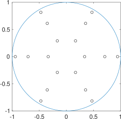
(a) $3\times 6$ nodes

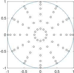
(b) $6\times 12$ nodes

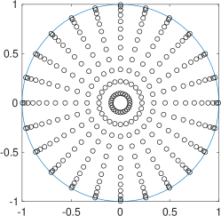
(c) $12\times 24$ nodes

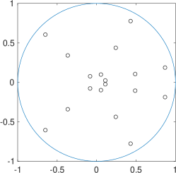
(d) $3\times 6$ nodes

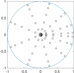
(e) $6\times 12$ nodes

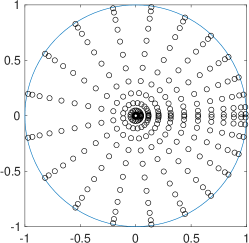
(f) $12\times 24$ nodes

Figure 3.1: Top panel: The distribution of quadrature nodes ($N_{r}\times N_{\theta}$) in the unit disk using the Elhay–Kautsky quadrature rule. Bottom panel: The distribution of quadrature nodes ($N_{\xi}\times N_{\eta}$) in the unit disk using the Gauss–Legendre quadrature rule.

Experimental results reveal that the Elhay–Kautsky quadrature (3.8) performs better in cases the interpolated function $f(x,y)$ is a bivariate polynomial, whereas the Gauss–Legendre quadrature (3.10) or the generalized Gaussian quadrature rule (see [Ma/Rokhlin/Wandzura:1996:GeneralizedQuadrature]) when $f(x,y)$ is an arbitrary nonlinear function.

In order to determine which quadrature rule performs better for the system (3.3), we perform a convergence test by applying the quadrature formulas (3.8) and (3.10) to the function $g_{1}(r)g_{2}(\theta,x,y)I_{0}(r,\theta)r$, where ${g_{1}(r)=100(-r+\delta)}$, $g_{2}(\theta,x,y)=\sin(\theta)+1$, and

$$I_{0}(r,\theta)=\frac{100}{2\pi\sigma^{2}}\exp\left(-\frac{r^{2}}{2\sigma^{2}}\right)$$

is a Gaussian distribution with deviation $\sigma$ and centered at zero. This resembles the initial conditions for $I$ at the origin, as we will use later in section 5sec:Numericssec:Numerics. The exact solution of the integral over a disk of radius $\delta$ is given by

$$\int_{0}^{\delta}\int_{0}^{2\pi}g_{1}(r)g_{2}(\theta)I_{0}\,r\,\mathrm{d}\theta\,\mathrm{d}r=5000\left(2\delta-\sqrt{2\pi}\,\sigma\,\text{erf}\left(\frac{\delta}{\sqrt{2}\sigma}\right)\right),$$ (3.11)

where $\text{erf}(x)$ is the Gauss error function [Andrews:1998:SpecialFunctions, William:2002:EconometricAnalysis]. Figure 3.2 shows the convergence of the two quadrature rules over the disk of radius $\delta$, as $\delta$ goes to zero ($\sigma=1/10$). We observe that the Gauss–Legendre quadrature (3.10) gives much smaller errors (close to machine precision) when more than $12\times 24$ nodes are used, compared to the Elhay–Kautsky quadrature (3.8) which is third-order accurate.

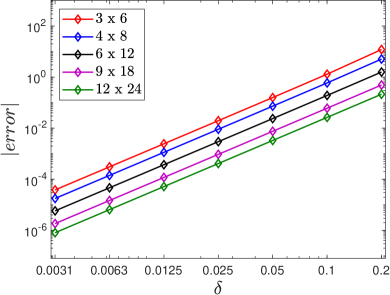
(a) Elhay–Kautsky quadrature (3.8)

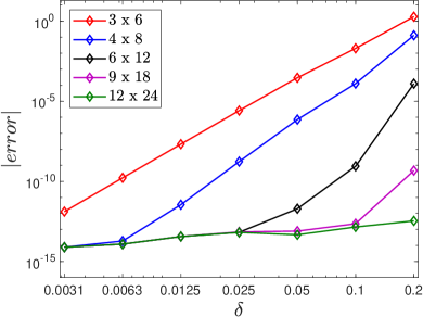
(b) Gauss–Legendre quadrature (3.10)

Figure 3.2: Numerical integration errors of quadrature formulas (3.8) and (3.10) applied to the integral in (3.11). The colored curves correspond to different choices of quadrature nodes in the $\delta$-radius disk.

The performance of the quadrature formulas depends also on the choice and accuracy of interpolation. As mentioned before, bilinear interpolation can be used since it preserves the non-negativity of the interpolant. One possibility is to use higher order interpolations, like cubic or spline, but in these cases the preservation of the required properties cannot be guaranteed. However, numerical experiments show that piecewise cubic spline interpolation results in a positive interpolant for a sufficiently fine spatial grid. A better choice is the use of a shape-preserving interpolation, to ensure that negative values are not generated and the interpolant of $I(t,\bar{x}_{k},\bar{y}_{l})$ in (3.4) is bounded by $\max_{k,l}\{S_{k,l}+I_{k,l}+R_{k,l}\}$ for every point $(x_{k},y_{l})$. This can be accomplished by a monotone interpolation that uses piecewise cubic Hermite interpolating polynomials [Dougherty/Edelman/Hyman:1989:HermiteInterpolation, Fritsch/Carlson:1980:MonotoneInterpolation]. In MATLAB (version R2021a) the relevant function is called pchip but is only available for one-dimensional problems. Extensions to bivariate shape-preserving interpolation have been studied in [Carlson/Fritsch:1985:MonotoneBicubic, Carlson:Fritsch:1989:MonotoneBicubicAlgorithm, Fritsch/Carlson:1985:MonotoneBicubicReport]; however, this topic goes beyond the purposes of this paper. Another choice is the modified Akima piecewise cubic Hermite interpolation, makima. Numerical experiments demonstrate good performance as it avoids overshoots when more than two consecutive nodes are constant [Akima:1970:Interpolation, Akima:1974:BivariateInterpolation], and hence preserves non-negativity in areas where $I(t,\bar{x}_{k},\bar{y}_{l})$ is close to zero.

4 Time integration methods

The next step is to use time integration methods to solve the system of ordinary differential equations (3.3). First, we study sufficient and necessary time-step restrictions such that the forward Euler method satisfies a discrete analogue of properties $C_{1}$–$C_{4}$, denoted below by $D_{1}$–$D_{4}$. Then, we discuss how high order SSP Runge–Kutta methods can be applied to (3.3).

Let $X^{n}=\{X^{n}_{k,l}\}$, $X\in\{S,I,R\}$, be the numerical approximation of $X_{k,l}(t_{n})$ for all ${1\leq k\leq P_{1}}$, $1\leq l\leq P_{2}$, and $0\leq n\leq\mathcal{N}$, where $\mathcal{N}$ is the total number of steps. The numerical solution should satisfy the following properties:

1. The densities $\{X^{n}_{k,l}\}$, $X\in\{S,I,R\}$, are non-negative for every $1\leq k\leq P_{1}$ , ${1\leq l\leq P_{2}}$, and for all $0\leq n\leq\mathcal{N}$.

2. The sum $S^{n}_{k,l}+I^{n}_{k,l}+R^{n}_{k,l}$ is constant for all $0\leq n\leq\mathcal{N}$ and for every $1\leq k\leq P_{1}$, $1\leq l\leq P_{2}$.

3. The density $S^{n}_{k,l}$ is non-increasing, i.e., $S^{n}_{k,l}\leq S^{n-1}_{k,l}$ for every $1\leq k\leq P_{1}$, $1\leq l\leq P_{2}$, and for all $1\leq n\leq\mathcal{N}$.

4. The density $R^{n}_{k,l}$ is non-decreasing i.e., $R^{n}_{k,l}\geq R^{n-1}_{k,l}$ for every $1\leq k\leq P_{1}$, $1\leq l\leq P_{2}$, and for all $1\leq n\leq\mathcal{N}$.

4.1 Explicit Euler scheme and qualitative properties

Let us apply the explicit Euler method to the system (3.3) on the interval $[0,t_{\text{f}}]$, and choose an adaptive time step $\tau_{n}>0$ such that $t_{n}=t_{n-1}+\tau_{n}$, $n\geq 1$. After the full discretization we get the set of algebraic equalities

$$S^{n} =S^{n-1}-\tau_{n}S^{n-1}\circ T^{n-1}-c\tau_{n}S^{n-1},$$ (4.1a)

$$I^{n} =I^{n-1}+\tau_{n}S^{n-1}\circ T^{n-1}-b\tau_{n}I^{n-1},$$ (4.1b)

$$R^{n} =R^{n-1}+b\tau_{n}I^{n-1}+c\tau_{n}S^{n-1}.$$ (4.1c)

Here, the operator $\circ$ denotes the element-by-element or Hadamard product of matrices. The matrix $T^{n-1}$ is an approximation of (3.4) at all points $(x_{k},y_{l})\in\mathcal{G}$, and its components can be expressed by

$$T_{k,l}^{n-1}=\sum_{(\bar{x}_{k},\bar{y}_{l})\in\mathcal{Q}_{\delta}(x_{k},y_{l})}w_{i,j}g_{1}(r_{i})g_{2}(\theta_{j},x_{k},y_{l})\tilde{I}^{n-1}(\bar{x}_{k},\bar{y}_{l}).$$ (4.2)

Now we examine the bounds of time step $\tau_{n}$ such that the method (4.1) gives solutions which are qualitatively adequate and satisfy conditions $D_{1}$–$D_{4}$.

Theorem 4.1.

Consider the numerical solution (4.1) obtained by the forward Euler method applied to (3.3) with non-negative initial data. Then, the solution satisfies property $D_{2}$ without any step-size restrictions. Moreover, properties $D_{1}$, $D_{3}$ and $D_{4}$ hold if the time step satisfies

$$\tau_{n}\leq\min\left\{\dfrac{1}{\max_{k,l}\{T_{k,l}^{n-1}\}+c},\dfrac{1}{b}\right\}.$$ (4.3)

Proof.

The proof is similar to the one of [Takacs/Horvath/Farago:2019:SpaceModelsDiseases, Theorem 2]. We prove the statement by induction on the number of steps.

First, assume that the properties $D_{1}$–$D_{4}$ hold up to step $n-1$; we will prove that they also hold true for step $n$. Property $D_{2}$ can be easily verified by adding all equations in (4.1). To show the monotonicity and non-negativity of $S^{n}$, consider (4.1a) at point $(x_{k},y_{l})\in\mathcal{G}$

$$S_{k,l}^{n}=\bigl{(}1-\tau_{n}(T_{k,l}^{n-1}+c)\bigr{)}S_{k,l}^{n-1}.$$

By our assumption $I_{k,l}^{n-1}\geq 0$, and a positivity-preserving interpolation guarantees that the interpolated values $\tilde{I}^{n-1}(\bar{x}_{k},\bar{y}_{l})=\tilde{I}^{n-1}\bigl{(}x_{k}+r_{i}\cos(\theta_{j}),y_{l}+r_{i}\sin(\theta_{j})\bigr{)}$ are non-negative. Therefore, by (4.2) we get $T_{k,l}^{n-1}\geq 0$ for each $1\leq k\leq P_{1}$ , $1\leq l\leq P_{2}$ since the weights $w_{i,j}$ are positive, and functions $g_{1}$ and $g_{2}$ are non-negative. As a result, $\tau_{n}(T_{k,l}^{n-1}+c)\geq 0$ and thus $S_{k,l}^{n}\leq S_{k,l}^{n-1}$. Moreover, if $\tau_{n}\leq 1/(T_{k,l}^{n-1}+c)$ then $S_{k,l}^{n}$ remains non-negative. Equation (4.1b) yields

$$I_{k,l}^{n}=(1-b\tau_{n})I_{k,l}^{n-1}+\tau_{n}S_{k,l}^{n-1}T_{k,l}^{n-1},$$

and hence $I^{n}$ is non-negative if $\tau_{n}\leq 1/b$. Finally from (4.1c) we have

$$R_{k,l}^{n}=R_{k,l}^{n-1}+b\tau_{n}I_{k,l}^{n-1}+c\tau_{n}S_{k,l}^{n-1},$$

therefore $R^{n}$ is non-negative and $R^{n}\geq R^{n-1}$. Putting all together we conclude that properties $D_{1}$–$D_{4}$ are satisfied if the time step is bounded by (4.3). By using the above argument it can be shown that $D_{1}$–$D_{4}$ also hold at the first step, $n=1$, if the initial data are non-negative and the time step satisfies (4.3). ∎

A drawback of the time-step restriction (4.3) is that it depends on the solution at the previous step. This has important complications for higher order methods as we will see in section 4.2subsec:RKsubsec:RK. For any multistage method, the adaptive time step bound (4.3) depends not only on the previous solution but also on the internal stage approximations. Consequently, an adaptive time-step restriction based on (4.3) cannot be the same for all stages of a Runge–Kutta method; instead it needs to be recalculated at every stage to guarantee that conditions $D_{1}$–$D_{4}$ hold. Therefore, such bound has no practical use because it is prone to rejected steps and will likely tend to zero.

A remedy is to use a constant time step that is less strict than (4.3), but still guarantee ${\tau\leq 1/(T_{k,l}^{n-1}+c)}$ holds for all $1\leq k\leq P_{1}$, $1\leq l\leq P_{2}$ and at every step $n$. At a given point $(x_{k},y_{l})\in\mathcal{G}$ the weights and quadrature nodes in $B_{\delta}(x_{k},y_{l})$ are the same regardless of the location of $(x_{k},y_{l})$ in the domain. Therefore, we can find an upper bound for each element of the matrix $T^{n-1}$ in (4.2). Let

$$\widehat{T}\coloneqq\sum_{(\bar{x}_{k},\bar{y}_{l})\in\mathcal{Q}_{\delta}(x_{k},y_{l})}w_{i,j}g_{1}(r_{i})\kappa_{2}M_{0},$$ (4.4)

where

$$M_{0}=\max_{(x_{k},y_{l})\in\mathcal{G}}\left\{S(0,x_{k},y_{l})+I(0,x_{k},y_{l})+R(0,x_{k},y_{l})\right\},$$ (4.5)

and $\kappa_{2}$ was defined before. Since $T_{k,l}^{n-1}\leq\widehat{T}$ for all $1\leq k\leq P_{1}$, $1\leq l\leq P_{2}$ then if

$$\widehat{\tau}\coloneqq\min\left\{\dfrac{1}{\widehat{T}+c},\dfrac{1}{b}\right\},$$ (4.6)

the condition

$$\widehat{\tau}\leq\min\left\{\dfrac{1}{\max_{k,l}\{T_{k,l}^{n-1}\}+c},\dfrac{1}{b}\right\}$$

holds at every step $n$. Moreover, $\widehat{T}\leq\widetilde{w}\,\kappa^{2}M_{0}N$, where

$$\kappa=\max\{\kappa_{1},\kappa_{2}\}=\max\left\{\max_{r\in(0,\delta)}\{g_{1}(r)\},\max_{\begin{subarray}{c}\theta\in[0,2\pi)\\ (x,y)\in\Omega\end{subarray}}\{g_{2}(\theta,x,y)\}\right\},$$

$\widetilde{w}=\max_{i,j}\{w_{i,j}\}$, and $N$ is the number of the quadrature nodes in $\mathcal{Q}_{\delta}(x_{k},y_{l})$. Hence, the time step (4.6) is larger than the rather pessimistic time step

$$\widetilde{\tau}\coloneqq\min\left\{\dfrac{1}{\widetilde{w}\,\kappa^{2}M_{0}N+c},\dfrac{1}{b}\right\},$$ (4.7)

proposed in [Takacs/Horvath/Farago:2019:SpaceModelsDiseases, Theorem 2]. Numerical experiments show that $\widehat{\tau}$ is very close to the theoretical bound in (4.3), and thus a relatively small increase of time step beyond the bound (4.6) may produce qualitatively bad solutions which violate one of the conditions $D_{1}$–$D_{4}$ (see section 5.1subsec:Eulercompsubsec:Eulercomp).

4.2 SSP Runge–Kutta methods

The forward Euler method is only first-order accurate; hence, we would like to obtain time-step restrictions for higher order Runge–Kutta methods. Note that the spatial discretizations discussed in section 3sec:Spatialsec:Spatial can be chosen so that errors from quadrature formulas and interpolation are very small; therefore, it is substantial to have a high-order accurate time integration method.

Consider a Runge–Kutta method in the Butcher form [Butcher:2016:ODEbook] with coefficients ${(a_{ij})\in\mathbb{R}^{m\times m}}$ and $\bm{b}\in\mathbb{R}^{m}$. Let $\mathcal{K}$ be the matrix given by

$$\mathcal{K}=\left[\begin{array}[]{cc}(a_{ij})&0\\ \bm{b}^{\intercal}&0\end{array}\right],$$

and denote by $I$ the $(m+1)$-dimensional identity matrix. If there exists $r>0$ such that $(I+r\mathcal{K})$ is invertible, then the Runge–Kutta method can be expressed in the canonical Shu–Osher form

$$\begin{split}Q^{(i)}&=v_{i}Q^{n-1}+\sum_{j=1}^{m}\alpha_{ij}\left(Q^{(j)}+\frac{\tau}{r}F\left(Q^{(j)}\right)\right),\qquad 1\leq i\leq m+1,\\ Q^{n}&=Q^{(m+1)},\end{split}$$ (4.8)

where the coefficient arrays $(\alpha_{ij})$ and $(v_{i})$ have non-negative components. Such methods are called strong-stability preserving (SSP) Runge–Kutta methods and have been introduced by Shu as total-variation diminishing (TVD) discretizations [Shu:1988:TVD], and by Shu and Osher in relation to high order spatial discretizations [Shu/Osher:1988:ENO, Shu:1998:ENO-WENO]. The choice of parameter $r$ gives rise to different Shu–Osher representations; thus we denote the Shu–Osher coefficients of (4.8) by $\bm{\alpha}_{r}=(\alpha_{ij})$ and $\bm{v}_{r}=(v_{i})$ to emphasize the dependence on the parameter $r$. The Shu–Osher representation with the largest value of $r$ such that $(I+r\mathcal{K})^{-1}$ exists and $\bm{\alpha}_{r}$, $v_{r}$ have non-negative components is called optimal and attains the SSP coefficient

$$\mathcal{C}=\max\left\{r\geq 0\;|\;\exists\;(I+r\mathcal{K})^{-1}\text{ and }\bm{\alpha}_{r}\geq 0,\bm{v}_{r}\geq 0\right\}.$$

The interested reader may consult [Gottlieb/Ketcheson/Shu:2009:HighOrderSSP, Gottlieb/Shu:1998:TVDRK, Gottlieb/Shu/Tadmor:2001:SSP], as well as the monograph [Gottlieb/Ketcheson/Shu:2011:SSPbook] and the references within, for a throughout review of SSP methods.

We would like to investigate time-step restrictions such that the numerical solution obtained by applying method (4.8) to the problem (3.3) satisfies properties $D_{1}$–$D_{4}$. The following theorem provides the theoretical upper bound for the time step such that these properties are satisfied.

Theorem 4.2.

Consider the numerical solution obtained by applying an explicit Runge–Kutta method (4.8) with SSP coefficient $\mathcal{C}>0$ to the semi-discrete problem (3.3) with non-negative initial data. Then property $D_{2}$ holds without any time-step restrictions. Moreover, the properties $D_{1}$, $D_{3}$ and $D_{4}$ hold if the time step satisfies

$$\tau\leq\mathcal{C}\min\left\{\dfrac{1}{\widehat{T}+c},\dfrac{1}{b}\right\},$$ (4.9)

where $\widehat{T}$ is given by (4.4).

Proof.

Consider an arbitrary stage $i$, $1\leq i\leq m+1$, of a Runge–Kutta method (4.8) with non-negative coefficients and SSP coefficient $\mathcal{C}>0$. Applying the method to (3.3) we get

$$S^{(i)} =v_{i}S^{n-1}+\sum_{j=1}^{i-1}\alpha_{ij}\left(S^{(j)}-\frac{\tau}{\mathcal{C}}\left(S^{(j)}\circ T^{(j)}-cS^{(j)}\right)\right),$$ (4.10a)

$$I^{(i)} =v_{i}I^{n-1}+\sum_{j=1}^{i-1}\alpha_{ij}\left(I^{(j)}+\frac{\tau}{\mathcal{C}}\left(S^{(j)}\circ T^{(j)}-bI^{(j)}\right)\right),$$ (4.10b)

$$R^{(i)} =v_{i}R^{n-1}+\sum_{j=1}^{i-1}\alpha_{ij}\left(R^{(j)}+\frac{\tau}{\mathcal{C}}\left(bI^{(j)}+cS^{(j)}\right)\right).$$ (4.10c)

Since all Runge–Kutta methods preserve linear invariants the property $D_{2}$, i.e.,

$$S^{n}+I^{n}+R^{n}=S^{n-1}+I^{n-1}+R^{n-1},\quad\forall n$$

is trivially satisfied.

The remainder of the proof deals with properties $D_{1}$, $D_{3}$ and $D_{4}$. We show that all quantities $S^{n},I^{n},R^{n}$ remain non-negative, while $S^{n}$ is non-increasing and $R^{n}$ is increasing. From (4.10a) and (4.10b) we have, respectively,

$$S^{(i)} =v_{i}S^{n-1}+\sum_{j=1}^{i-1}\alpha_{ij}S^{(j)}\circ\left(\mathbf{1}-\frac{\tau}{\mathcal{C}}\left(T^{(j)}+c\mathbf{1}\right)\right),$$

$$I^{(i)} =v_{i}I^{n-1}+\frac{\tau}{r}\sum_{j=1}^{i-1}\alpha_{ij}S^{(j)}\circ T^{(j)}+\left(1-\frac{\tau}{r}b\right)\sum_{j=1}^{i-1}\alpha_{ij}I^{(j)},$$

where $\mathbf{1}$ is the $P_{1}\times P_{2}$ all-ones matrix.

By definition,

$$T_{k,l}^{(i)}=\sum_{(\bar{x}_{k},\bar{y}_{l})\in\mathcal{Q}_{\delta}(x_{k},y_{l})}w_{i,j}g_{1}(r_{i})g_{2}(\theta_{j},x_{k},y_{l})\tilde{I}^{(i)}(\bar{x}_{k},\bar{y}_{l}),\qquad 1\leq i\leq m+1,$$

where $\tilde{I}^{(i)}$ are interpolated values. Since the initial data are non-negative and the chosen interpolation is positivity-preserving, we have that $S^{(1)}=S^{n-1}$, $I^{(1)}=I^{n-1}$ and $T^{(1)}$ are all non-negative. If

$$0\leq 1-\dfrac{\tau}{r}b,\text{ and }0\leq\mathbf{1}-\frac{\tau}{\mathcal{C}}\left(T^{(j)}+c\mathbf{1}\right)\text{ for }1\leq j\leq i-1,$$ (4.11)

then the explicit Runge–Kutta method inductively results in non-negative $T^{(i)}$, $S^{(i)}$, and $I^{(i)}$ for each $2\leq i\leq m+1$. Since $\tilde{I}^{(i)}(\bar{x}_{k},\bar{y}_{l})$ is an interpolated value of $I^{(i)}(\bar{x}_{k},\bar{y}_{l})$ it is bounded by $M_{0}$ (see (4.5)). Then by using (4.4), it holds that $T^{(i)}_{k,l}\leq\widehat{T}$, for $1\leq i\leq m+1$ and for every $(x_{k},y_{l})\in\mathcal{G}$. Therefore,

$$T^{(i)}\leq\widehat{T}\mathbf{1},\quad 1\leq i\leq m+1.$$ (4.12)

Moreover, the non-negativity of $T^{(i)}$ implies that

$$\mathbf{1}-\frac{\tau}{\mathcal{C}}\left(T^{(i)}+c\mathbf{1}\right)\leq 1,\quad 1\leq i\leq m+1,$$

and thus (4.10a) yields $S^{(i)}\leq v_{i}S^{n-1}+\sum_{j=1}^{i-s}\alpha_{ij}S^{(j)}$. Consistency requires that $v_{i}+\sum_{j=1}^{i-1}\alpha_{ij}=1$ for each $1\leq i\leq m+1$ and hence

$$\begin{split}S^{(i)}&\leq(1-\sum_{j=1}^{i-1}\alpha_{ij})S^{n-1}+\sum_{j=1}^{i-1}\alpha_{ij}S^{(j)}\\ &\leq S^{n}-\sum_{j=1}^{i-1}\alpha_{ij}\left(S^{n-1}-S^{(j)}\right).\end{split}$$ (4.13)

Let $1\leq q\leq m+1$ be the stage index such that $S^{(i)}\leq S^{(q)}$ for all $1\leq i\leq m+1$. Then, taking $i=q$ in (4.13) yields

$$S^{(q)} \leq v_{i}S^{n-1}+\sum_{j=1}^{i-1}\alpha_{qj}S^{(q)}$$

$$\left(1-\sum_{j=1}^{i-1}\alpha_{qj}\right)S^{(q)} \leq\left(1-\sum_{j=1}^{i-1}\alpha_{qj}\right)S^{n-1}$$

$$S^{(q)} \leq S^{n-1}.$$

Therefore, $S^{(i)}\leq S^{n-1}$ for all $1\leq i\leq m+1$. In particular for $i=m+1$ we have ${S^{n}=S^{(m+1)}\leq S^{n-1}}$.

Finally, the non-negativity of initial data, $S^{(j)}$ and $I^{(j)}$ implies that from (4.10c) we have $R^{(i)}\geq R^{n-1}$ for all $1\leq i\leq m+1$, and hence $R^{n}=R^{(m+1)}\geq R^{n-1}$.

Combining (4.11) and (4.12) we conclude that the step-size restriction (4.9) is sufficient for satisfying properties $D_{1}$–$D_{4}$. ∎

5 Numerical experiments

In this section, we confirm the results proved previously by using several numerical experiments. Computational tests are defined in a bounded domain and thus the choice of boundary conditions is important. Because we have no diffusion in our problem, we consider homogeneous Dirichlet conditions and we assume that there is no susceptible population outside of the domain. This means that we are going to assign a zero value to any point which lies outside of the rectangular domain in which the problem is defined. In most cases, the nodes of the quadrature rules (3.8) and (3.10) do not belong to the spatial grid. Special attention must be given to the corners and boundaries of the domain where quadrature nodes, assigned to grid points near the boundary, lie outside of the domain. In order to handle solution estimates at corners and the boundary of the domain, we use ghost cells which are set to zero Thus, we can calculate the values corresponding to the quadrature nodes lying outside of the domain without violating the qualitative properties. All code to generate the figures and tables discussed in this section is available at https://github.com/hadjimy/spatial-SIR_RR.

For the numerical experiments we are choosing the following functions. Let $g_{1}(r)$ be a linearly decreasing function, which takes its maximum at $r=0$ and becomes zero at $r=\delta$, i.e.,

$$g_{1}(r)\coloneqq a(-r+\delta),$$

where $a$ is the same parameter as in (1.1). The $g_{2}(\theta,x_{k},y_{l})$ function is given by

$$g_{2}(\theta,x_{k},y_{l})\coloneqq\beta_{k,l}\left(\sin\left(\frac{\pi}{2}+\theta-\alpha_{k,l}\right)+\beta_{0}\right),$$ (5.1)

where $\alpha_{k,l}$ describes the wind’s direction at point $(x_{k},y_{l})$ and $\beta_{k,l}$ is the strength of the wind. The parameter $\beta_{0}$ is set to $11/10$ to ensure that $g_{2}(\theta,x_{k},y_{l})$ is strictly positive. We use a differentiable velocity field to resemble a wind profile on the domain $\Omega=[0,\mathcal{L}_{1}]\times[0,\mathcal{L}_{2}]$, and hence at each grid point $(k,l)$ the wind direction is given by a vector $\bm{\upsilon_{k,l}}=(\upsilon^{1}_{k,l},\upsilon^{2}_{k,l})$, (see Figure 5.1(c)). The parameter $\alpha_{k,l}$ denotes the angle of the wind vector $\bm{\upsilon_{k,l}}$ with the positive $x$-axis, and $\beta_{k,l}$ is calculated by the $L^{2}$-norm of $\bm{\upsilon_{k,l}}$.

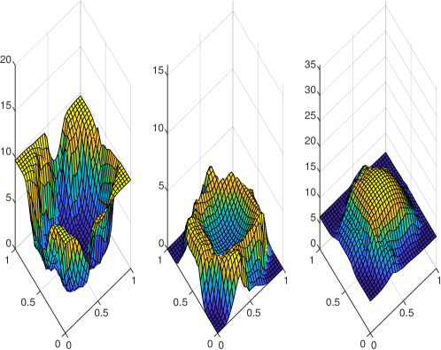
(a) $t=50$

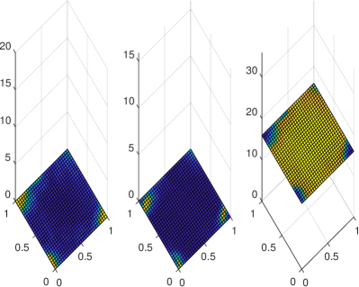
(b) $t=1000$

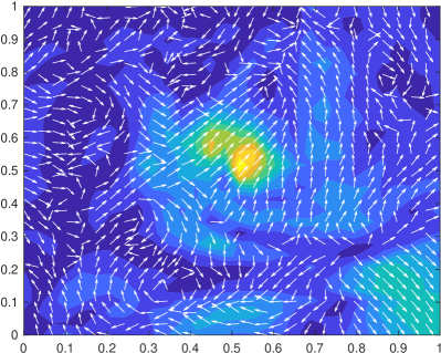
(c) wind profile; the colors indicate the intensity of the wind

Figure 5.1: The number of susceptibles $S$ (left), infected $I$ (middle) and recovered $R$ (right) at times $t=50$ (top panel) and $t=1000$ (bottom panel). The Gauss–Legendre quadrature (3.10) has been used combined with the makima interpolation. Plot (c) shows the wind velocity field used.

The initial conditions resemble the eruption of a wildfire, i.e., having infected cases located in a small area. For the infected species, we use a Gaussian distribution concentrated at the middle point $\left(\mathcal{L}_{1}/2,\mathcal{L}_{2}/2\right)$ of the domain $\Omega$, with standard deviation $\sigma=\min\{\mathcal{L}_{1},\mathcal{L}_{2}\}/10$. The spatial step sizes are $h_{1}=\mathcal{L}_{1}/(P_{1}-1)$ and $h_{2}=\mathcal{L}_{2}/(P_{2}-1)$, where $P_{1}$ and $P_{2}$ are the number of grid points in each direction. We assume that the number of susceptibles is constant except at the middle of the domain, and there are no recovered species at the beginning. Therefore, for every $1\leq k\leq P_{1}$, $1\leq l\leq P_{2}$ the initial conditions are given by

$$I_{k,l}^{0} =\dfrac{1}{2\pi\sigma^{2}}\exp\left(-\dfrac{1}{2}\left[\left(\dfrac{h_{1}(k-1)-\dfrac{\mathcal{L}_{1}}{2}}{\sigma}\right)^{2}+\left(\dfrac{h_{2}(l-1)-\dfrac{\mathcal{L}_{2}}{2}}{\sigma}\right)^{2}\right]\right),$$

$$S_{k,l}^{0} =\dfrac{1}{2\pi\sigma^{2}}-I_{k,l}^{0},$$

$$R_{k,l}^{0} =0.$$

In all numerical experiments - unless otherwise stated - we use the parameter values $a=100$, $b=0.05$, $c=0.01$, and $\delta=0.05$. The computational domain is $\Omega=[0,1\times[0,1]$ with $30$ grid points in each direction, and we use $6\times 12$ quadrature nodes. We also choose the tenth-stage, fourth-order SSP Runge–Kutta method (SSPRK104) for the time integration.

First we would like to study the behavior of our numerical solution. Figure 5.1 depicts the numerical solution at times $t=50$ and $t=1000$. As we can see, the number of susceptibles is decreased, and the number of infected moves towards the boundaries, while forming a wave. Both densities $S$ and $I$ tend to zero, which confirms that the zero solution is indeed an asymptotically stable equilibrium for the first two equations of (1.4).

5.1 Comparison of the step size bounds for the Euler method

As seen in section 4.1subsec:FEsubsec:FE, the improved bound $\widehat{\tau}$ (see (4.6)) is larger than the pessimistic bound $\widetilde{\tau}$ (see (4.7)), and thus closer to the best theoretically bound (4.3) that guarantees the preservation of properties $D_{1}$–$D_{4}$. We would like to determine how close the bound $\widehat{\tau}$ is to the adaptive step-size restriction, and compare it with the pessimistic bound $\widetilde{\tau}$. In Table 5.1 we have tested several different values of $a$ and $\delta$, for which both the bounds $\widehat{\tau}$ and $\widetilde{\tau}$ were computed. For comparison we calculated the minimum of the adaptive step bound (4.3), denoted by $\tau_{e}$. As we can see, varying the parameter $a$ or $\delta$ the time-step bound $\widehat{\tau}$ results in about $50\%$ increase in efficiency compared to $\widetilde{\tau}$. Also, the time-step restriction $\widehat{\tau}$ is much closer to the theoretical bound for which the properties $D_{1}$–$D_{4}$ hold. From Table 5.1 we conclude that in the case of a small increase in the time step $\widehat{\tau}$, the forward Euler method continues to preserve the desired properties. However, for values of $\tau$ bigger than (4.9), there is no guarantee that properties $D_{1}$–$D_{4}$ will be satisfied by a high-order time integration method.

$a$	$\widetilde{\tau}$	$\widetilde{\tau}/\tau_{e}$	$\widehat{\tau}$	$\widehat{\tau}/\tau_{e}$	$\tau_{e}$
$50$	$2.7934$	$0.4267$	$6.0609$	$0.9259$	$6.5462$
$100$	$1.4165$	$0.4186$	$3.1252$	$0.9235$	$3.3839$
$250$	$0.5715$	$0.4136$	$1.2740$	$0.9221$	$1.3816$
$500$	$0.2865$	$0.4193$	$0.6411$	$0.9381$	$0.6833$

$\delta$	$\widetilde{\tau}$	$\widetilde{\tau}/\tau_{e}$	$\widehat{\tau}$	$\widehat{\tau}/\tau_{e}$	$\tau_{e}$
$0.025$	$10.310$	$0.5155$	$20.000$	$1.0000$	$20.000$
$0.050$	$1.4165$	$0.4186$	$3.1252$	$0.9235$	$3.3839$
$0.075$	$0.4239$	$0.4096$	$0.9468$	$0.9149$	$1.0349$
$0.100$	$0.1793$	$0.4168$	$0.4016$	$0.9337$	$0.4301$

Table 5.1: Step-size bounds $\widehat{\tau}$ and $\widetilde{\tau}$ (see (4.6) and (4.7) respectively), and their comparison with the adaptive bound $\tau_{e}$ (see (4.3)) for the forward Euler method for different values of $a$ and $\delta$. The computation uses the Elhay–Kautsky quadrature rule (3.10) combined with bilinear interpolation, and the final time is $t_{\text{f}}=100$.

5.2 Convergence

Since we cannot approximate the exact solution accurately, we are going to compute the numerical errors for different methods by using a reference solution. To have a fair comparison the reference solution is computed by using the same parameters and method, but with either a large number of quadrature nodes or a very small time step.

We first observe how well the different quadratures behave. As seen in section 3sec:Spatialsec:Spatial, using more nodes in quadrature (3.10) results in smaller errors, and also faster convergence. Numerical experiments show that this is also the case for the system (3.3). The $L^{2}$-norm errors for the different quadrature formulas and interpolations are plotted in Figure 5.2. It is clear that for a small number of quadrature nodes there is no remarkable difference between the interpolations, but for more quadrature nodes makima and spline interpolation perform better. Bilinear interpolation results in similar errors for both quadratures (3.8) and (3.10). The makima and spline interpolations have a similar performance for the Elhay–Kautsky quadrature (3.8) and smaller errors are observed with spline interpolation and Gauss–Legendre quadrature (3.10). Notice, thought that spline interpolation does not guarantee the preservation of properties $D_{1}$–$D_{4}$, e.g., setting $\beta_{0}=1$ in (5.1) yields negative values for the infected density $I$.

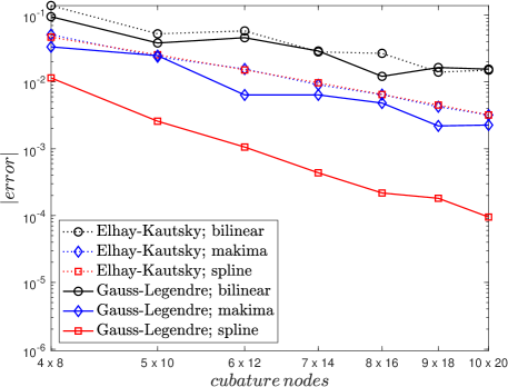
Figure 5.2: $L^{2}$-norm errors using quadrature formulas (3.8) and (3.10) with $n\times 2n$ quadrature nodes, $n\in\{4,5,6,7,8,9,10\}$ and different interpolations. The final time is $t_{\text{f}}=50$ and the reference solution for each quadrature rule and interpolation is computed by using $20\times 40$ quadrature nodes.

Equally important is the order of the different time integration methods. Table 5.2 shows that the forward Euler method behaves similarly when compared to the first-order integral solution described in section 2.2subsec:InteqralSolutionsubsec:InteqralSolution. Numerical experiments show that the higher order schemes work as expected, namely that by using enough quadrature nodes and grid points, a reasonably small error can be achieved with the desired accuracy order. Table 5.3 shows the convergence rates for second-, third- and fourth-order SSP Runge–Kutta methods when the Gauss–Legendre quadrature rule (3.10) is used with spline interpolation. The numerical solution is computed at time $t_{\text{f}}=50$ using $30$ grid points and $6\times 12$ quadrature nodes. We start with a reasonable time step $4.7$, which is slightly below the minimum of the adaptive bound (4.3) when forward Euler method is used, and then successively divide by $2$. For the reference solution we use a time step that is the half of the smallest time step in our computations. It is evident that using higher order methods is better than solving the integral equation (2.12) numerically. Moreover the fourth-order SSP Runge–Kutta method (SSPRK104) attends a six times larger time step than lower order methods since it has an SSP coefficient $\mathcal{C}=6$.

$\tau$	FE		IM
$0.8250$	$4.35\times 10^{-1}$		$1.74\times 10^{0}$
$0.4125$	$2.26\times 10^{-1}$	$0.94$	$1.19\times 10^{0}$	$0.54$
$0.2062$	$1.14\times 10^{-1}$	$0.99$	$7.32\times 10^{-1}$	$0.70$
$0.1031$	$5.59\times 10^{-2}$	$1.03$	$4.07\times 10^{-1}$	$0.85$
$0.0516$	$2.62\times 10^{-2}$	$1.09$	$2.06\times 10^{-1}$	$0.98$
$0.0258$	$1.13\times 10^{-2}$	$1.22$	$9.22\times 10^{-2}$	$1.16$

Table 5.2: $L^{2}$-norm errors and convergence rates of forward Euler method (FE) and the method (2.14), denoted by “IM”. The solution is computed at time $t_{\text{f}}=50$ with the Gauss–Legendre quadrature rule (3.10) combined with spline interpolation.

$\tau$	SSPRK22		SSPRK33		SSPRK104
$3.3000$	$2.93\times 10^{-1}$		$4.45\times 10^{-2}$		$4.71\times 10^{-4}$
$1.6500$	$9.08\times 10^{-2}$	$1.69$	$7.13\times 10^{-3}$	$2.64$	$3.30\times 10^{-5}$	$3.84$
$0.8250$	$2.53\times 10^{-2}$	$1.84$	$1.01\times 10^{-3}$	$2.82$	$2.18\times 10^{-6}$	$3.92$
$0.4125$	$6.63\times 10^{-3}$	$1.93$	$1.35\times 10^{-4}$	$2.91$	$1.40\times 10^{-7}$	$3.96$
$0.2062$	$1.63\times 10^{-3}$	$2.03$	$1.72\times 10^{-5}$	$2.97$	$8.82\times 10^{-9}$	$3.99$
$0.1031$	$3.29\times 10^{-4}$	$2.30$	$1.94\times 10^{-6}$	$3.15$	$5.19\times 10^{-10}$	$4.09$

Table 5.3: $L^{2}$-norm errors and convergence rates of high-order integration methods. The solution is computed at time $t_{\text{f}}=50$ with the Gauss–Legendre quadrature rule (3.10) combined with spline interpolation.

5.3 Runtime comparison

The spatial discretization (interpolation and quadrature rule) is expected to be the dominant computation load for the numerical solution of (3.3). We estimate the elapsed time of the numerical solvers for the spatial discretizations; this includes the calculation of the improved step-size bound $\widehat{\tau}$ (see (4.6)) at the setup of the simulation and all calculations per step for the interpolation and quadrature formulas. Table 5.4 compares the time required (in seconds) for the spatial discretization and the overall computation time. The parameters, initial conditions, computational domain, and the number of grid points and quadrature nodes are the same as at the beginning of this section. We use three Runge–Kutta methods (forward Euler, SSPRK33, and SSPRK104) combined with the bilinear and makima interpolation and compute the solution at a final time $t_{\text{f}}=50$. We choose the Gauss–Legendre quadrature (3.10) with for all tests as it is slightly faster than the Elhay–Kautsky quadrature. As shown in Table 5.4 the time needed for the spatial discretization is almost equal to the overall time of the simulations. Also, the bilinear interpolation is twice as fast as the makima interpolation. The forward Euler method uses a single function evaluation per step; hence it is the fastest among all methods. There is a linear increase in computation time with the three-stage SSPRK33 method because it has the same SSP coefficient as the forward Euler method but requires three function evaluations per step. The SSPRK104 method uses ten function evaluations per step; however, it has six times larger step-size bound than forward Euler and thus it takes only about twice as much time. The additional computation effort of the SSPRK104 method is compensated by a fourth-order accurate solution.

method	interpolation	time (s)
		spatial discretization	total runtime
FE	bilinear	$1.417$	$1.453$
	makima	$3.599$	$3.607$
SSPRK33	bilinear	$3.964$	$3.974$
	makima	$10.596$	$10.606$
SSPRK104	bilinear	$2.579$	$2.593$
	makima	$6.871$	$6.878$

Table 5.4: Elapsed time of the spatial discretization compared to the overall simulation time. The computations use different Runge–Kutta methods and interpolations, combined with the Gauss–Legendre quadrature (3.10) with $30$ grid points in each direction and $6\times 12$ quadrature nodes. The final time is $t_{\text{f}}=50$.

6 Conclusions and further work

In this paper, the SIR model for epidemic propagation is extended to include spatial dependence. The existence and uniqueness of the continuous solution are proved, along with properties corresponding to biological observations. For the numerical solution, different choices of quadrature, interpolation, and time integration methods are studied. It is shown that for a sufficiently small time-step restriction, the numerical solution preserves a discrete analog of the properties of the original continuous system. The step-size bound is improved compared to previous results. An adaptive step-size technique is also suggested for the explicit Euler method, and we have determined step-size bounds for higher order methods. Analytic results are confirmed by numerical experiments, while the errors of quadrature formulas and the order of accuracy of the time discretization methods are also discussed.

The work presented in this paper can be extended to diffusion spatial-dependent SIR systems, and also include the effect of fractional diffusion. Results for the preservation of qualitative properties of such a system could be potentially obtained in a similar fashion as in the current manuscript. Moreover, the inclusion the births and natural deaths in the system and dropping the conservation property could make the model more realistic. Several biological and epidemiological metrics, for instance, the basic reproduction number, could be also estimated. It would be interesting to study the influence of such modification in the behavior of the continuous and also the numerical solution.

Appendix A Proofs of lemmata in section 2sec:Analyticalsec:Analytical

We present the proofs of some technical lemmata that were omitted in the previous sections.

Proof of Lemma 2.1.

The statement simply follows from

$$\left\lVert u\right\rVert^{2}=c^{2}\dfrac{1}{c^{2}}\left\lVert u_{1}\right\rVert_{L^{2}}^{2}+b^{2}\dfrac{1}{b^{2}}\left\lVert u_{2}\right\rVert_{L^{2}}^{2} \leq\max\left\{\dfrac{1}{b^{2}},\dfrac{1}{c^{2}}\right\}\left(c^{2}\left\lVert u_{1}\right\rVert_{L^{2}}^{2}+b^{2}\left\lVert u_{2}\right\rVert_{L^{2}}^{2}\right)$$

$$=\left(\frac{1}{\min\{b,c\}}\right)^{2}\left\lVert u\right\rVert_{A}^{2},$$

and

$$\left\lVert u\right\rVert_{A}^{2}=c^{2}\left\lVert u_{1}\right\rVert_{L^{2}}^{2}+b^{2}\left\lVert u_{2}\right\rVert_{L^{2}}^{2}\leq\max\{b^{2},c^{2}\}(\left\lVert u_{1}\right\rVert_{L^{2}}^{2}+\left\lVert u_{2}\right\rVert_{L^{2}}^{2})=\max\{b,c\}^{2}\left\lVert u\right\rVert^{2}.$$

∎

Proof of Lemma 2.2.

We are going to derive an upper bound to the term

$$\left\lVert\mathcal{F}(u_{2})\right\rVert_{L^{2}}^{2} =\bigintsss_{\Omega}\bigg{|}\int_{0}^{\delta}\int_{0}^{2\pi}g_{1}(r)g_{2}(\theta,x,y)u_{2}\bigl{(}t,\bar{x}(r,\theta),\bar{y}(r,\theta)\bigr{)}\,r\,\mathrm{d}\theta\,\mathrm{d}r\bigg{|}^{2}\!\,\mathrm{d}x\,\mathrm{d}y$$

$$=\bigintsss_{\Omega}\bigg{|}\int_{B_{\delta}(\mathbf{x})}g_{1}(r)g_{2}(\theta,x,y)u_{2}(t,\bar{\mathbf{x}})\,\mathrm{d}\bar{\mathbf{x}}\bigg{|}^{2}\!\,\mathrm{d}\mathbf{x},$$

where we used the notation $\bar{\mathbf{x}}\coloneqq\bigl{(}\bar{x}(r,\theta),\bar{y}(r,\theta)\bigr{)}=\bigl{(}x+r\cos(\theta),y+r\sin(\theta)\bigr{)}$, and $B_{\delta}(\mathbf{x})$ is the ball with radius $\delta$ around $\mathbf{x}$. By the definition of $g_{1}$ and $g_{2}$, we have that

$$\left\lVert\mathcal{F}(u_{2})\right\rVert_{L^{2}}^{2}=\bigintsss_{\Omega}\bigg{|}\int_{\Omega}g_{1}(r)g_{2}(\theta,\mathbf{x})u_{2}(t,\tilde{\mathbf{x}})\,\mathrm{d}\tilde{\mathbf{x}}\bigg{|}^{2}\,\mathrm{d}\mathbf{x}.$$

We also know that $g_{1}$ and $g_{2}$ are bounded. Using the notations $\kappa_{1}=\max_{r\in(0,\delta)}\{g_{1}(r)\}$ and $\kappa_{2}=\max_{\theta\in[0,2\pi),\mathbf{x}\in\Omega}\{g_{2}(\theta,\mathbf{x})\}$, yields

$$\left\lVert\mathcal{F}(u_{2})\right\rVert_{L^{2}}^{2} =\bigintsss_{\Omega}\bigg{|}\int_{\Omega}1\cdot g_{1}(r)g_{2}(\theta,\mathbf{x})u_{2}(t,\tilde{\mathbf{x}})\,\mathrm{d}\tilde{\mathbf{x}}\bigg{|}^{2}\!\,\mathrm{d}\mathbf{x}$$

$$\leq\!\!\!\bigintss_{\Omega}\bBigg@{2.8}|\sqrt{\int_{\Omega}1^{2}\,\mathrm{d}\tilde{\mathbf{x}}}\;\sqrt{\int_{\Omega}\big{(}g_{1}(r)g_{2}(\theta,\mathbf{x})u_{2}(t,\tilde{\mathbf{x}})\big{)}^{2}\,\mathrm{d}\tilde{\mathbf{x}}}\bBigg@{2.8}|^{2}\!\,\mathrm{d}$$

$$\leq\mu(\Omega)\int_{\Omega}\int_{\Omega}\bigl{|}g_{1}(r)g_{2}(\theta,\mathbf{x})u_{2}(t,\tilde{\mathbf{x}})\bigr{|}^{2}\,\mathrm{d}\tilde{\mathbf{x}}\,\mathrm{d}\mathbf{x}$$

$$\leq\kappa_{1}^{2}\,\kappa_{2}^{2}\,\mu(\Omega)\int_{\Omega}\int_{\Omega}\bigl{|}u_{2}(t,\tilde{\mathbf{x}})\bigr{|}^{2}\,\mathrm{d}\tilde{\mathbf{x}}\,\mathrm{d}\mathbf{x},$$

where we used the Cauchy–Schwarz inequality, and $\mu(\Omega)$ is the Lebesgue measure of $\Omega$. It holds that

$$\int_{\Omega}\int_{\Omega}\bigl{|}u_{2}(t,\tilde{\mathbf{x}})\bigr{|}^{2}\,\mathrm{d}\tilde{\mathbf{x}}\,\mathrm{d}\mathbf{x}=\int_{\Omega}\left\lVert u_{2}\right\rVert_{L^{2}}^{2}\,\mathrm{d}\mathbf{x}=\mu(\Omega)\left\lVert u_{2}\right\rVert_{L^{2}}^{2}.$$

Consequently,

$$\left\lVert\mathcal{F}(u_{2})\right\rVert_{L^{2}}\leq\kappa_{1}\,\kappa_{2}\,\mu(\Omega)\left\lVert u_{2}\right\rVert_{L^{2}},$$

and setting $\nu_{\mathcal{F}}=\kappa_{1}\kappa_{2}\,\mu(\Omega)$ we get the result of the lemma. ∎

Proof of Lemma 2.3.

Consider the system (2.9a)-(2.9b) written in the compact form (2.1), where $A$ is given by (2.4), $F$ is defined in (2.5), and the corresponding norm $\left\lVert\cdot\right\rVert$ is given by (2.2). Let $\{\varepsilon_{i}\}$ and $\{\varepsilon_{j}\}$ be two sequences such that $\lim_{i\rightarrow\infty}\varepsilon_{i}=0$ and $\lim_{j\rightarrow\infty}\varepsilon_{j}=0$. Assume that $u_{\varepsilon_{i}}(t)$ and $u_{\varepsilon_{j}}(t)$ are solutions of (2.9a)-(2.9b), and define the vectors $\widehat{\varepsilon_{i}}\coloneqq(0,\varepsilon_{i})^{\intercal}$ and $\widehat{\varepsilon_{j}}\coloneqq(0,\varepsilon_{j})^{\intercal}$ Then

$$u^{\prime}_{\varepsilon_{i}}(t)-u^{\prime}_{\varepsilon_{j}}(t)=A(u_{\varepsilon_{i}}(t)-u_{\varepsilon_{j}}(t))+F(u_{\varepsilon_{i}}(t))-F(u_{\varepsilon_{j}}(t))+\widehat{\varepsilon_{i}}-\widehat{\varepsilon_{j}}.$$

Using the definition of $A$ and Corollary 2.1, yields

$$\left\lVert u^{\prime}_{\varepsilon_{i}}(t)-u^{\prime}_{\varepsilon_{j}}(t)\right\rVert \leq\left\lVert A(u_{\varepsilon_{i}}(t)-u_{\varepsilon_{j}}(t))\right\rVert+\left\lVert F(u_{\varepsilon_{i}}(t))-F(u_{\varepsilon_{j}}(t))\right\rVert+\left\lVert\widehat{\varepsilon_{i}}-\widehat{\varepsilon_{j}}\right\rVert$$

$$\leq\bigl{(}\left\lVert A\right\rVert+\zeta(d)\bigr{)}\left\lVert u_{\varepsilon_{i}}(t)-u_{\varepsilon_{j}}(t)\right\rVert+\left\lVert\widehat{\varepsilon_{i}}-\widehat{\varepsilon_{j}}\right\rVert,$$

where $\zeta(d)$ is defined in Corollary 2.1. By Grönwall’s inequality (see [Halanay:ODEs:1966, Lemma 1.6]), we have

$$\left\lVert u_{\varepsilon_{i}}(t)-u_{\varepsilon_{j}}(t)\right\rVert\leq\left\lVert\widehat{\varepsilon_{i}}-\widehat{\varepsilon_{j}}\right\rVert t+\left\lVert\int_{0}^{t}\bigl{(}\left\lVert A\right\rVert+\zeta(d)\bigr{)}\;(\widehat{\varepsilon_{i}}-\widehat{\varepsilon_{j}})\;t\exp\left(\int_{s}^{t}\bigl{(}\left\lVert A\right\rVert+\zeta(d)\bigr{)}\;\,\mathrm{d}w\right)\,\mathrm{d}s\right\rVert.$$

Since we assume that $\lim_{i,j\rightarrow\infty}\varepsilon_{i}-\varepsilon_{j}=0$, the statement is proved. ∎

Appendix B List of symbols and notations

Symbol	Description
$S(t,x,y)$, $I(t,x,y)$, $R(t,x,y)$	density functions of susceptible, infected and recovered species
$a$, $b$, $c$	parameters describing the rate of infection, recovery, and vaccination
$\delta$	parameter describing the radius of the effect of an infectious individual
$g_{1}(r)$, $g_{2}(\theta,x,y)$	functions describing the effect of an infectious individual to its surroundings
$E=L^{2}(\Omega)\times L^{2}(\Omega)$	Hilbert-space for the solution of system (2.1)
$\left\lVert\cdot\right\rVert$	norm of Hilbert-space $E$ defined in (2.2)
$\left\lVert\cdot\right\rVert_{A}$	operator norm of $D(A)$ defined in (2.3)
$A:D(A)\rightarrow E$	linear part of equation (1.4)
$F:D(A)\rightarrow E$	non-linear part of equation (1.4)
$\mathcal{F}$	the integral term in (1.4)