Bias and Consistency in Three-way Gravity Models

We study the incidental parameter problem for the “three-way” Poisson Pseudo-Maximum Likelihood (“PPML”) estimator recently recommended for identifying the effects of trade policies and in other panel data gravity settings. Despite the number and variety of fixed effects involved, we confirm PPML is consistent for fixed $T$ and we show it is in fact the only estimator among a wide range of PML gravity estimators that is generally consistent in this context when $T$ is fixed. At the same time, asymptotic confidence intervals in fixed-$T$ panels are not correctly centered at the true point estimates, and cluster-robust variance estimates used to construct standard errors are generally biased as well. We characterize each of these biases analytically and show both numerically and empirically that they are salient even for real-data settings with a large number of countries. We also offer practical remedies that can be used to obtain more reliable inferences of the effects of trade policies and other time-varying gravity variables, which we make available via an accompanying Stata package called ppml_fe_bias.

JEL Classification Codes: C13; C50; F10
Keywords: Structural Gravity; Trade Agreements; Asymptotic Bias Correction

1 Introduction

Despite intense and longstanding empirical interest, the effects of bilateral trade agreements on trade are still considered highly difficult to assess. As emphasized in a recent practitioner’s guide put out by the WTO (Yotov, Piermartini, Monteiro, and Larch, 2016), many current estimates in the literature suffer from easily identifiable sources of bias (or “estimation challenges”). This is not for a lack of awareness. Papers showing leading causes of bias in the gravity equation are often among the most widely celebrated and cited in the trade field, if not in all of Economics. In particular, it is now generally accepted that trade flows across different partners are interdependent via the network structure of trade (the main contribution of Anderson and van Wincoop, 2003), that log-transforming the dependent variable is not innocuous (as argued by Santos Silva and Tenreyro, 2006), and—most relevant to the context of trade agreements—that earlier, puzzlingly small estimates of the effects of free trade agreements were almost certainly biased downwards by treating them as exogenous (Baier and Bergstrand, 2007).

As a consequence—and aided by some recent computational developments—researchers seeking to identify the effects of trade agreements have naturally moved towards more advanced estimation strategies that take on board all of the above concerns. In particular, a “three-way” fixed effects Poisson Pseudo-Maximum Likelihood (“FE-PPML”) estimator with time-varying exporter and importer fixed effects to account for network dependence and time-invariant exporter-importer (“pair”) fixed effects to address endogeneity has recently emerged as a logical workhorse method for empirical trade policy analysis. It also has clear potential application to the study of network data more generally, such as data on urban commuting or migration (e.g., Brinkman and Lin, 2019; Gaduh, Grac̆ner, and Rothenberg, 2020; Allen, Dobbin, and Morten, 2018; Beverelli and Orefice, 2019).

However, one reason why some researchers may hesitate in embracing this estimator is the current lack of clarity regarding how the three fixed effects in the model may bias estimation, especially in the standard “fixed $T$” case where the number of time periods is small. Even though FE-PPML estimates can be shown to be asymptotically unbiased with a single fixed effect (a well-known result) as well as in a two-way setting where both dimensions of the panel become large (Fernández-Val and Weidner, 2016), the latter result does not come strictly as a generalization of the former one, leaving it potentially unclear whether a three-way model with a fixed time dimension should be expected to inherit the nice asymptotic properties of these other models.

Accordingly, the question we investigate in this paper is the extent to which the three-way FE-PPML estimator is affected by incidental parameter problems (IPPs). As is well known in both statistics and econometrics (Neyman and Scott, 1948; Lancaster, 2002), IPPs arise when estimation noise from estimates of fixed effects and other “incidental parameters” contaminates the scores of the main parameters of interest, inducing bias. In the worst case, this bias renders the estimates inconsistent, making estimation inadvisable. As we will show, while inconsistency is actually not a problem for three-way FE-PPML, both the estimated coefficients and standard errors are affected by meaningful biases due to IPPs that researchers should be aware of.

To state our main results more precisely, in gravity settings where the number of countries ($N$) goes to infinity and $T$ is small, we find the following:

1. Consistency of point estimates of FE-PPML: The point estimates produced by three-way FE-PPML estimator in gravity settings are asymptotically consistent.

2. Inconsistency of other FE-PML estimators: FE-PPML is the only estimator in a set of related FE-PML estimators sometimes considered in this context that is generally consistent. FE-Gamma PML, for example, should not be used because it is only consistent under strict assumptions.

3. Asymptotic bias: Point estimates of the three-way FE-PPML estimator are nonetheless asymptotically biased, meaning that the asymptotic distribution of the estimates is not centered at the truth as $N\rightarrow\infty$. In other words, it approaches the truth “at an angle” asymptotically (see Figure 1 for an illustration.)

4. Biased standard error estimates: Estimates of cluster-robust sandwich-type standard errors are likewise asymptotically biased due to an IPP.

5. Bias corrections improve inferences: Simulations show that using analytical bias corrections to address each of these biases leads to improved inferences. These corrections are available to use via the Stata package ppml_fe_bias.

To first explain our consistency results, our basic strategy involves using the first-order conditions of FE-PPML to “profile out” (solve for) the pair fixed effect terms from the first-order conditions of the other parameters. Notably, this allows us to re-express the three-way gravity model as a two-way model in which the only remaining incidental parameters are the exporter-time and importer-time fixed effects. Three-way FE-PPML is therefore consistent in fixed-$T$ settings for largely the same reasons the two-way models considered in Fernández-Val and Weidner (2016) are consistent, and we provide suitably modified versions of the regularity conditions and consistency results established by Fernández-Val and Weidner (2016) for the simpler two-way case.

At the same time, it does not also follow that Fernández-Val and Weidner (2016)’s earlier results for the asymptotic unbiased-ness of the two-way FE-PPML estimator similarly carry over to the three-way case when $T$ is fixed. The key is that the resulting two-way estimator that is obtained after profiling out the fixed effects has its own special properties with respect to IPPs. When $T$ is fixed, the estimation noise in the remaining exporter-time and importer-time fixed effects induces an asymptotic bias of order $1/N$ as $N$ grows large, a result that is broadly consistent with most of the two-way settings studied in Fernández-Val and Weidner (2016). However, when instead both $N$ and $T$ grow large at the same rate, the estimator turns out to be unbiased asymptotically, analogous to what Fernández-Val and Weidner (2016) found in the two-way FE-PPML case.

The reason why asymptotic bias is a concern is that the asymptotic standard deviation is itself of order $1/(N\sqrt{T})$. Thus, when $T$ is fixed, both the bias in point estimates will be of comparable magnitude to their standard errors as $N\rightarrow\infty$, causing the asymptotic distribution of estimates to be incorrectly centered as discussed above. In practice, this is a less severe problem than inconsistency, but it does mean that standard hypothesis tests for assessing statistical significance are not reliable. One of the objectives of this paper will be to adapt some of the leading remedies from the recent literature on “large $T$” IPPs (see, e.g., Arellano and Hahn, 2007) in order to re-center the asymptotic distribution of estimates and thereby restore asymptotically valid inferences.

The bias in the estimated standard errors is similar to one that has been found in two-way gravity settings by several recent studies (Egger and Staub, 2015; Jochmans, 2016; Pfaffermayr, 2019, 2021). Intuitively, because the origin-time and destination-time fixed effects in the model each converge to their true values at a rate of only $1/\sqrt{N}$ (not $1/N$), the cluster-robust sandwich estimator for the variance has a leading bias of order $1/N$ (not $1/N^{2}$), and standard errors in turn have a bias of order $1/\sqrt{N}$. This latter type of bias is related to the general result that standard “heteroskedasticity-robust” variance estimators are downward-biased in small samples (see, e.g., MacKinnon and White, 1985; Imbens and Kolesar, 2016), including for PML estimators (Kauermann and Carroll, 2001), but is more severe in this setting due to an IPP. We should therefore be concerned that estimated confidence intervals may be too narrow in addition to being off-center.

For the bias in point estimates, we construct two-way analytical and jackknife bias corrections inspired by the corrections proposed in Fernández-Val and Weidner (2016; 2018). For the bias in standard errors, we show how Kauermann and Carroll (2001)’s method for correcting the PML sandwich estimator may be adapted to the case of a conditional estimator with multi-way fixed effects and cluster-robust standard errors. Our simulations confirm that these methods are usually effective at improving inferences. The jackknife correction reduces more of the bias in point estimates than the analytical correction in smaller samples, but the analytical correction does a better job at improving coverage, especially when also paired with corrected standard errors.

For our empirical applications, we first estimate the average effects of a free trade agreement (FTA) on trade for a range of different industries using what would typically be considered a large trade data set, with 167 countries and 5 time periods. The biases we uncover vary in size across the different industries, but are generally large enough to indicate that our bias corrections should be worthwhile in most three-way gravity settings. For aggregate trade data (which yields results that are fairly representative), the estimated coefficient for FTA has an implied downward bias about 15%-22% of the estimated standard error, and the implied downward bias in the standard error itself is about 11% of the original standard error. As a means of further demonstration, we also apply our corrections to replication data from several recent papers that have used three-way gravity models. This latter exercise reveals several instances in which our methods make a material difference for assessing statistical significance. It also highlights the possibility that the bias in standard errors can sometimes be severe, as much as 40% or more in some cases.

Aside from Fernández-Val and Weidner (2016)’s work on two-way nonlinear models, Pesaran (2006), Bai (2009), Hahn and Moon (2006), and Moon and Weidner (2017) have each conducted similar analyses for two-way linear models with interacted individual and time fixed effects. Turning to three-way models, Hinz, Stammann, and Wanner (2019) have recently developed bias corrections for dynamic three-way probit and logit models based on asymptotics suggested by Fernández-Val and Weidner (2018) where all three panel dimensions grow at the same rate. Though widely applicable, this approach is not appropriate for our setting because of the different role played by the time dimension when the estimator is FE-PPML. In the network context, Graham (2017), Dzemski (2018), and Chen, Fernández-Val, and Weidner (2019) have studied asymptotic bias in network models with node-specific (possibly sender- and receiver-specific) fixed effects. Chen, Fernández-Val, and Weidner (2019)’s analysis is espeically notable in that they allow these node-specific effects to be vectors rather than scalars, similar to the exporter-time and importer-time fixed effects that feature in gravity models. Our bias expansions substantially differ from those of Chen, Fernández-Val, and Weidner (2019) because the equivalent outcome variable in our setting (trade flows observed over time for a given pair) is also a vector rather than a scalar and because we work with a conditional moment model where the distribution of the outcome may be misspecified.

In what follows, Section 2 first provides a discussion of why IPPs are a concern for gravity models and of the no-IPP properties of FE-PPML. Section 3 then establishes bias and consistency results for the three-way gravity model specifically and discusses how to implement bias corrections. Sections 4 and 5 respectively present simulation evidence and empirical applications. Section 6 concludes, and an Appendix adds further simulation results and technical details, including proofs.

2 Gravity Models and IPPs

Gravity models are now routinely estimated using FE-PPML with multiple sets of fixed effects. As we discuss in this section, these practices follow naturally from the gravity model’s theoretical microfoundations but are not without need for further scrutiny. In particular, because the underlying model is nonlinear, it is important to clarify that, while PPML is known to be free from incidental parameter bias in some special cases, it is by no means immune to IPPs in general. It will also be useful for us to provide some general discussion of IPPs and the different ways in which they may manifest.

2.1 Fixed Effects and Gravity Models

As documented in Head and Mayer (2014), the emergence of rich and varied theoretical foundations for the gravity equation has fueled a “fixed effects revolution” in the gravity literature over the last two decades. As such, we find it useful to briefly describe a simple trade model and discuss how it may be used to motivate an estimating equation with either two-way or three-way fixed effects.

To establish some notation we will use throughout the paper, we will consider a world with $N$ countries and we will let $i$ and $j$ respectively be indices for exporter and importer. For now, we will focus on deriving a two-way gravity model where the two fixed effects account for each country’s multilateral resistance. Later, we will add a time dimension and a third fixed effect that absorbs all time-invariant components of trade costs.

To add some theoretical structure, suppose that trade flows are given by the following gravity equation:

$$y_{ij} =\frac{y_{i}}{\Pi_{i}^{-\theta}}\frac{y_{j}}{P_{j}^{-\theta}}\tau_{ij}^{-\theta}.$$ (1)

Here, $y_{i}:=\sum_{j}y_{ij}$ and $y_{j}:=\sum_{i}y_{ij}$ are the market sizes of the two countries, $\tau_{ij}\geq 1$ is a bilateral trade cost, $\theta>0$ is the trade elasticity, and $\Pi_{i}$ and $P_{j}$ respectively are the outward and inward multilateral resistances from Anderson and van Wincoop (2003), which capture how bilateral trade flows depend on each country’s opportunities for trade with third countries. More formally, these latter terms are derived from the following two relationships that are inherent to all general equilibrium gravity models:

$$\Pi_{i}^{-\theta} =\sum_{j=1}^{N}\frac{y_{j}}{P_{j}^{-\theta}}\tau_{ij}^{-\theta}, P_{j}^{-\theta} =\sum_{i=1}^{N}\frac{y_{i}}{\Pi_{i}^{-\theta}}\tau_{ij}^{-\theta}.$$ (2)

As shown, these terms respectively aggregate the exporter’s ability to export goods to more desirable import markets and the importer’s ability to import from more capable exporters.

For estimation, it is typical to parameterize the trade cost $\tau_{ij}$ as depending exponentially on some variables of interest, i.e.,

$$\tau_{ij}^{-\theta} =\exp(x_{ij}\beta)\omega_{ij},$$ (3)

where $x_{ij}$ are the components of trade costs whose effects we wish to estimate. Because not all trade costs are reflected in $x_{ij}$, we also allow for “unobserved” trade costs via the idiosyncratic trade cost term $\omega_{ij}$. Combining (1) with (3) then delivers the following estimating equation:

$$y_{ij} =\exp\left(\alpha_{i}+\gamma_{j}+x_{ij}\beta\right)\omega_{ij},$$ (4)

where $\alpha_{i}=\ln(y_{i}/\Pi_{i}^{-\theta})$ and $\gamma_{j}=\ln(y_{j}/P_{j}^{-\theta})$ are origin and destination fixed effects that absorb market sizes and multilateral resistances and $\omega_{ij}$ now provides a multiplicative error term. When we introduce the three-way model, all of the terms shown in (4) will have a further subscript for time, and the the unobserved trade cost will have a time-invariant component that will motivate the use of an added $ij$ fixed effect.

To motivate the arc of the rest of the paper, several points stand out from the estimation suggested by (5). First, the implied moment condition for estimation is

$$\mathbb{E}(y_{ij}|x_{ij},\alpha_{i},\gamma_{j}) =\lambda_{ij}:=\exp\left(\alpha_{i}+\gamma_{j}+x_{ij}\beta\right),$$ (5)

which follows after imposing $\mathbb{E}(\omega_{ij}|x_{ij},\!\alpha_{i},\!\gamma_{j})=1.$ As discussed in Santos Silva and Tenreyro (2006), consistent estimation of the trade cost parameters in $\beta$ therefore generally requires a nonlinear model. Second, because unobserved trade costs enter the country-specific terms $\alpha_{i}$ and $\gamma_{j}$ through the system of multilateral resistances, we treat $\alpha_{i}$ and $\gamma_{j}$ as unknown parameters that will be noisily estimated, raising concerns about a possible IPP. As we go on to discuss, the FE-PPML estimator that is most often used in this context has some special robustness against IPPs, but this robustness does not hold for FE-PPML in general, especially once we deviate from the two-way gravity setting implied by (5).

2.2 The Incidental Parameter Problem

In the context of fixed effects models, IPPs occur when the estimation noise in the fixed effects contaminates the scores of the other parameters being estimated, inducing a bias. This bias can manifest in a variety of different ways; thus it is useful to provide a generic characterization that can illustrate the different possibilities that may arise. To that end, let $n$ be the total number of observations and let $p$ be the total number of parameters being estimated, inclusive of any fixed effects. As described in Fernández-Val and Weidner (2018), what we need to be concerned with the number of observations that are available to estimate each fixed effect, i.e., $n/p$. More precisely, when appropriate regularity conditions are satisfied, the estimated $\widehat{\beta}$ may generally be thought of as having the following bias and standard deviation:

$${\rm bias}(\widehat{\beta}) =\frac{b\,p}{n}+o(p/n), {\rm std}(\widehat{\beta}) =\frac{c}{\sqrt{n}}+o(n^{-1/2}),$$ (6)

where $b\in\mathbb{R}$ and $c>0$ are constants that depend on the model being estimated. As this presentation emphasizes, all estimators in nonlinear settings are generally biased in small samples, but this is not the same thing as saying that the bias always poses a problem for inferring statistical significance. As we will discuss, in larger samples, what matters is whether the bias disappears faster than the standard error as $n\rightarrow\infty.$

To provide a simple taxonomy of the cases that can arise, consider first the standard textbook treatment of maximum likelihood estimation, where we usually have $p$ fixed while $n\rightarrow\infty$. In this case, the bias in $\widehat{\beta}$ becomes asymptotically negligible as compared to the standard deviation, which crucially means that estimated confidence intervals can be expected to be centered at the truth when the data becomes sufficiently large. By contrast, in the classical IPP of Neyman and Scott (1948), the number of parameters grows at the same rate as the number of observations, implying that the bias does not converge to zero asymptotically. In that case, the fixed effect estimator is inconsistent.

The gravity model with two-way fixed effects then serves to illustrate a third possibility that will also be applicable to the results that follow for three-way gravity models. In the two-way gravity setting, $p$ is on the order of $2N$, where $N$ is the number of countries, and $n$ is on the order of $N^{2}$. Consequently, the bias and standard deviation of $\widehat{\beta}$ are given by

$${\rm bias}(\widehat{\beta}) =\frac{2\,b}{N}+o(1/N), {\rm std}(\widehat{\beta}) =\frac{c}{N}+o(1/N),$$ (7)

In this case, as $N\rightarrow\infty$, the estimated $\widehat{\beta}$ is consistent (both the standard deviation and bias converge to zero), but we also have

$$\lim_{N\rightarrow\infty}\;\frac{{\rm bias}(\widehat{\beta})}{{\rm std}(\widehat{\beta})}=\frac{2\,b}{c}.$$

As we discuss below, the two-way PPML gravity estimator is a special case where we actually have that $b=0$. However, for other two-way gravity estimators (such as two-way Gamma PML for example), we generally have that $b\neq 0$, meaning the bias will not disappear relative to the standard error as $N\rightarrow\infty$. Compared to Neyman and Scott (1948), the IPP these estimators suffer from is not an inconsistency problem but rather an asymptotic bias problem, whereby the slow convergence of the fixed effects causes the asymptotic distribution for $\widehat{\beta}$ to be incorrectly centered as it converges to the truth. This version of the IPP is more benign, but ignoring the bias will nonetheless result in invalid inferences and test results. The “large $T$” panel data literature therefore discusses various methods for bias correction of $\widehat{\beta}$ that restore asymptotically valid inference. Importantly, the degree to which inferences are biased depends on the bias constant $b$, which cannot be known beforehand without applying such a correction.

To provide a more visual illustration of these ideas, Figure 1 presents simulation results for the three cases we have just discussed: inconsistency (top-left), no asymptotic bias (top-right), and asymptotic bias (bottom-left). Since asymptotic bias will ultimately be our focus, it is worth noting from the figure how the estimates are consistent in this case—the distribution will collapse to the true value as $N\rightarrow\infty$—but confidence bounds based on these estimates will clearly be inappropriate.

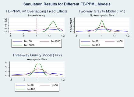
Figure 1: Kernel density plots of FE PPML estimates for 3 different models, using 500 replications. Clockwise from top left, the 3 models are: $y_{it}=\exp[\alpha_{i}\times 1(t\leq 2)+\gamma_{i}\times 1(t\geq 2)+x_{it}\beta]\omega_{it}$, with the $t$ dimension of the panel fixed at $T=3$; a two-way gravity model with $y_{ij}=\exp[\alpha_{i}+\gamma_{j}+x_{ij}\beta]\omega_{ij}$; a three-way gravity model with $y_{ijt}=\exp[\alpha_{it}+\gamma_{jt}+\eta_{ij}+x_{ijt}\beta]\omega_{ijt}$ and $T=2$. Respectively, these models exemplify inconsistency, no asymptotic bias, and asymptotic bias. The $i$ and $j$ dimensions of the panel both have size $N$ in the latter two models. The true value of $\beta$ is 1 (indicated by the vertical dotted lines) and the data is generated using ${\rm Var}(y|\cdot)=\mathbb{E}(y|\cdot)$.

2.3 How FE-PPML is Different

Our discussion of IPPs thus far has been for the generic estimation of a nonlinear model. However, the PPML estimator that is most commonly used to estimate gravity models actually behaves very differently than other estimators in this context. In the classic panel data setting with “one way” fixed effects, for example, FE-PPML has the very special property that the IPP bias constant $b$ turns out to be zero, meaning that it is asymptotically unbiased in situations where other estimators tend to be inconsistent. As discussed in Wooldridge (1999), the reason behind this result is that the same estimator can be obtained from a multinomial model that does not depend on the fixed effects.

This special property of FE-PPML has important implications for estimating gravity models as well. For two-way gravity settings, the asymptotic bias of $\widehat{\beta}$ when $N\rightarrow\infty$ was worked out in Fernández-Val and Weidner (2016). They show that the two IPP contributions from $\alpha_{i}$ and $\gamma_{j}$ “decouple” asymptotically, such that the overall bias can be decomposed as the sum of two bias terms that would be expected in a one-way setting, i.e., $b_{(\alpha)}/N+b_{(\gamma)}/N$, where the $N$’s come from the number of observations associated with each fixed effect. Because $b=0$ for the one-way FE-PPML case, we also have $b_{(\alpha)}=b_{(\gamma)}=0$ in the two-way setting; that is, two-way FE-PPML gravity estimates for $\widehat{\beta}$ are asymptotically unbiased just as one-way FE-PPML estimates are.

Taken together, these results might create the impression that FE-PPML is generally immune to IPPs, regardless of what fixed effects are included in the model. Thus, it is important to clarify that a key feature of the two-way gravity model is that both fixed effect dimensions grow only with the square root of the panel size, such that the estimation noise in the estimated $\widehat{\alpha}_{i}$’s and $\widehat{\gamma}_{j}$’s disappears asymptotically. As we discuss in the Appendix, if we instead consider a model where both fixed effects grow with $n$ rather than with its square root, the IPPs associated with each fixed effect do not decouple from one another, and FE-PPML in this case is actually inconsistent.

To synthesize these points, FE-PPML has a very special property—one can condition out one of the fixed effects—but this property has an important limitation—the resulting multinomial model does not inherit the same no-bias properties as the original PPML estimator with respect to any further fixed effects. Both of these results will be fleshed out in more detail in the following section when we recast the three-way gravity model as a two-way multinomial model in order to obtain an appropriate expression for the bias. Doing so will also allow us to highlight another reason why FE-PPML is not immune to IPPs: even for the two-way gravity model, while the $\alpha_{i}$ and $\gamma_{j}$ parameters do not induce an IPP bias in $\widehat{\beta}$, they nonetheless have implications for the estimated variance that are not innocuous; we thus will devote attention to this issue as well.

3 Results for the Three-way Gravity Model

To recap the sequence of results just described, we know that FE-PPML estimates with one fixed effect do not suffer from an IPP. We also know that FE-PPML may have an IPP in models with more than one fixed effect, but it is both consistent and asymptotically unbiased in two-way gravity settings where neither fixed effect dimension grows at the same rate as the size of the panel. As we will now show, each of these earlier results will be useful for understanding the more complex case of a three-way gravity model that adds a time dimension and a third set of fixed effects to the above two-way model. We also describe a series of bias corrections for the three-way model, including for the possible downward bias of the estimated standard errors.

3.1 Consistency

To formally introduce the three-way model, we add an explicit time subscript $t\in\{1,\ldots,T\}$ to $y_{ij}$, $x_{ij}$, and $\omega_{ij}$ from the prior model and add a “country-pair”-specific fixed effect $\eta_{ij}$, such that trade costs are now given by $\tau_{ijt}^{-\theta}=e^{x_{ijt}^{\prime}\beta+\eta_{ij}}\omega_{ijt}$. All other elements in the original trade model likewise acquire a time subscript, meaning that $\alpha_{it}=\ln{y_{it}/\Pi_{it}^{-\theta}}$ and $\gamma_{jt}=\ln{y_{jt}/P_{jt}^{-\theta}}$ also must be indexed by $t$. The model now reads

$$\mathbb{E}(y_{ijt}|x_{ijt},\alpha_{it},\gamma_{jt},\eta_{ij}) =\lambda_{ijt}:=\exp(x_{ijt}^{\prime}\beta+\alpha_{it}+\gamma_{jt}+\eta_{ij}),$$ (8)

where the three fixed effects now respectively index exporter-time, importer-time, and country-pair. The unobserved trade cost $\omega_{ijt}\geq 0$ continues to serve as an error term, such that $y_{ijt}=\lambda_{ijt}\omega_{ijt}\geq 0$. We thus allow for zero trade flows. For the asymptotics using the three-way model, we consider $T$ fixed, while $N\rightarrow\infty$. The FE-PPML estimator maximizes

$$\mathcal{L}(\beta,\alpha,\gamma,\eta) :=\sum_{i=1}^{N}\sum_{\begin{minipage}[c]{15.6491pt} $\scriptstyle j=1$ \\ $\scriptstyle j\neq i$ \end{minipage}}^{N}\sum_{t=1}^{T}\left(y_{ijt}\log\lambda_{ijt}-\lambda_{ijt}\right)$$

over $\beta$, $\alpha$, $\gamma$ and $\eta$.

Our strategy for showing the consistency of this estimator will capitalize on the special properties of FE-PPML discussed in the previous section. In particular, we will exploit the fact that not all of the fixed effect dimensions grow at the same rate as $N$ increases. The numbers of exporter-time and importer-time fixed effects each increase with $N$ (as before), but the dimension of the pair fixed effect $\eta$ increases with $N^{2}$, since adding another country to the data adds another $N-1$ pairs to the estimation. It therefore makes sense to first “profile out” (i.e., solve for) $\eta$ so that we may deal with the remaining two fixed effects in turn. For given values of $\beta$, $\alpha$, $\gamma$, maximizing over $\eta$ gives us

$$\exp\left[\widehat{\eta}_{ij}(\beta,\alpha,\gamma)\right] =\frac{\sum_{t=1}^{T}y_{ijt}}{\sum_{t=1}^{T}\mu_{ijt}}, \mu_{ijt} :=\exp(x_{ijt}^{\prime}\beta+\alpha_{it}+\gamma_{jt}).$$ (9)

We therefore have

$$\mathcal{L}(\beta,\alpha,\gamma) :=\max_{\eta}\mathcal{L}(\beta,\alpha,\gamma,\eta)=\sum_{i=1}^{N}\sum_{\begin{minipage}[c]{15.6491pt} $\scriptstyle j=1$ \\ $\scriptstyle j\neq i$ \end{minipage}}^{N}\ell_{ij}(\beta,\alpha_{it},\gamma_{jt}),$$ (10)

with

$$\ell_{ij}(\beta,\alpha_{it},\gamma_{jt}) :=\sum_{t=1}^{T}y_{ijt}\log\left(\frac{\mu_{ijt}}{\sum_{s=1}^{T}\mu_{ijs}}\right)+\text{terms not depending on parameters},$$ (11)

thus leaving us with the likelihood of a multinomial model where the only incidental parameters are $\alpha_{it}$ and $\gamma_{jt}$. Using (8), one can easily verify that there is no bias in the score of the profile log-likelihood $\ell_{ij}(\beta,\alpha_{it},\gamma_{jt})$ when evaluated at the true parameters $\beta^{0}$, $\alpha_{it}^{0}$, and $\gamma_{jt}^{0}$. The reason for this is exactly the same as for the classic panel data setting discussed above. Furthermore, the remaining fixed effects $\alpha_{it}$ and $\gamma_{jt}$ grow only with the square root of the sample size as $N\rightarrow\infty$, implying that they are consistently estimated. This in turn leads us to the following result:

Proposition 1.

So long as the set of non-fixed effect regressors $x_{ijt}$ is exogenous to the disturbance $\omega_{ijt}$ after conditioning on the fixed effects $\alpha_{it}$, $\gamma_{jt}$, and $\eta_{ij}$, FE-PPML estimates of $\beta$ from the three-way gravity model are consistent for $N\rightarrow\infty$.

Intuitively, this result follows because of how the special properties of FE-PPML allow us to rewrite the three-way gravity model as a two-way model without introducing a $1/T$ bias. The form of the bias in $\widehat{\beta}$ is therefore the same as in (7), such that three-way FE-PPML is consistent as $N\rightarrow\infty$ largely for the same reason two-way FE-PPML and other two-way PML gravity estimators are generally consistent. However, in the context of three-way estimators, we can also state a stronger result that applies more narrowly to FE-PPML in particular:

Proposition 2.

Assume the conditional mean is given by $\lambda_{ijt}=\exp(x_{ijt}^{\prime}\beta+\alpha_{it}+\gamma_{jt}+\eta_{ij})$ and consider the class of “three-way” FE-PML gravity estimators with FOC’s given by

$$\widehat{\beta}\!\!:\,\sum_{i=1}^{N}\sum_{\begin{minipage}[c]{15.6491pt} $\scriptstyle j=1$ \\ $\scriptstyle j\neq i$ \end{minipage}}^{N}\sum_{t=1}^{T}\,\!x_{ijt}\!\left(y_{ijt}-\widehat{\lambda}_{ijt}\right)\!g(\widehat{\lambda}_{ijt}) =0, \widehat{\alpha}_{it}\!\!:\,\sum_{j=1}^{N}\left(y_{ijt}-\widehat{\lambda}_{ijt}\right)\!g(\widehat{\lambda}_{ijt}) =0,$$

$$\widehat{\gamma}_{jt}\!\!:\,\sum_{i=1}^{N}\left(y_{ijt}-\widehat{\lambda}_{ijt}\right)\!g(\widehat{\lambda}_{ijt}) =0, \widehat{\eta}_{ij}\!\!:\,\sum_{t=1}^{T}\left(y_{ijt}-\widehat{\lambda}_{ijt}\right)\!g(\widehat{\lambda}_{ijt}) =0,$$

where $i,j=1,\ldots,N$, $t=1,...,T,$ and $g(\widehat{\lambda}_{ijt})$ is an arbitrary function of $\widehat{\lambda}_{ijt}$ that can be specialized to construct various PML estimators. For example, $g(\widehat{\lambda}_{ijt})=1$ delivers PPML, $g(\widehat{\lambda}_{ijt})=\widehat{\lambda}_{ijt}^{-1}$ delivers Gamma PML, etc. If $T$ is fixed, then for $\widehat{\beta}$ to be consistent under general assumptions about ${\rm Var}(y|x,\alpha,\gamma,\eta)$, we must have that $g(\lambda_{ijt})$ is constant over the range of $\lambda$’s that are realized in the data-generating process. That is, the estimator must be equivalent to FE-PPML.

In other words, three-way FE-PPML is unique among three-way PML estimators in that its consistency does not require strong assumptions about the conditional variance of $y_{ijt}$. To draw an appropriate contrast, it is possible to obtain a closed form solution for the pair fixed effect $\widehat{\eta}_{ij}$ so long as $g(\widehat{\lambda}_{ijt})$ is of the form $g(\widehat{\lambda}_{ijt})=\widehat{\lambda}_{ijt}^{q}$, where $q$ can be any real number. Notably, this latter class of estimators not only includes FE-PPML (for which $q=0$), but also includes other popular gravity estimators such as Gamma PML ($q=-1$) and Gaussian PML ($q=1$). However, as we discuss in the Appendix, these other estimators are only consistent if the conditional variance is proportional to ${\lambda}_{ijt}^{1-q}$, in which case they inherit the properties of their associated MLE estimators.

3.2 Asymptotic Bias

Because three-way FE-PPML inherits the consistency properties of the two-way estimator, one might expect that it also inherits its “no asymptotic bias” properties as well. However, this is where the limitations of PPML’s no-IPP properties become apparent. While the profile log-likelihood in (10) is now of a similar form to the two-way models considered in Fernández-Val and Weidner (2016), notice that it no longer resembles the original FE-PPML log-likelihood. Their no-bias result for two-way FE-PPML therefore does not carry over to the three-way model, and it is possible to show that FE-PPML estimates have an asymptotic bias in this setting.

Before proceeding, it is helpful to first revisit the intuition established in Section 2.2 that shapes how we expect the bias to behave. As we have discussed, in a model with $p$ parameters and $n$ observations, the bias should be proportional to $p/n$, whereas the standard error should vary with $1/\sqrt{n}$. After profiling out $\eta$, the resulting two-way model has $\sim 2NT$ parameters vs. $\sim N^{2}T$ observations. If $T$ is held fixed, we would expect the bias and the standard error to decrease at the same rate ($1/N$), raising concerns about a possible asymptotic bias problem and guiding us as to its form. Readers should keep this intuition in mind in reading through the technical details that follow.

To illustrate more precisely where the bias comes from, it is necessary to examine how the estimated fixed effects enter the score for ${\beta}$ using a Taylor expansion. To that end, first let $\phi:={\rm vec}(\alpha,\gamma)$ be a vector that collects all of the exporter-time and importer-time fixed effects, such that we can rewrite $\ell_{ij}$ slightly as $\ell_{ij}=\ell_{ij}(\beta,\phi)$. We can then similarly define the function $\widehat{\phi}(\beta)$ as collecting the estimated fixed effects $\widehat{\alpha}$ and $\widehat{\gamma}$ as functions of $\beta$. Next, we construct a second-order expansion of the score for ${\beta}$ around the true set of fixed effects $\phi^{0}$ and evaluated at the true parameter $\beta^{0}$:

$$\mathbb{E}\left[\frac{\partial\ell_{ij}(\beta^{0},\widehat{\phi}(\beta^{0}))}{\partial\beta}\right] \approx\underbrace{\mathbb{E}\left[\frac{\partial\ell_{ij}(\beta^{0},\phi^{0})}{\partial\beta}\right]}_{=0}+\underbrace{\mathbb{E}\left[\frac{\partial^{2}\ell_{ij}(\beta^{0},\phi^{0})}{\partial\beta\partial\phi^{\prime}}\left(\widehat{\phi}(\beta^{0})-\phi^{0}\right)\right]}_{\neq 0\text{ (reflects estimation error in FEs)}}$$

$$+\underbrace{\frac{1}{2}\sum_{f,g}^{\dim\phi}\mathbb{E}\left[\frac{\partial^{3}\ell_{ij}(\beta^{0},\phi^{0})}{\partial\beta\partial\phi_{f}\partial\phi_{g}}\left(\widehat{\phi}_{f}(\beta^{0})-\phi_{f}^{0}\right)\left(\widehat{\phi}_{g}(\beta^{0})-\phi_{g}^{0}\right)\right]}_{\neq 0\text{ (reflects variances and covariances of FEs)}}.$$ (12)

This expression is near-identical to a similar expansion that appears in Fernández-Val and Weidner (2016)—differing mainly in that $\ell_{ij}$ is a vector rather than a scalar—and communicates the same essential insights: because the latter two terms in (12) are generally not equal to zero, the score for ${\beta}$ is biased, with the bias depending on the interaction between the higher-order partial derivatives of $\ell_{ij}$ and the estimation errors in $\widehat{\alpha}_{i}$ and $\widehat{\gamma}_{j}$ as well as their variances and covariances.

Demonstrating the bias in this particular setting then requires that we introduce some additional notation, mainly to provide some shorthand for the higher-order partial derivatives of $\ell_{ij}$ that appear in (12). To do so, we first find it convenient to let $\vartheta_{ijt}:=\lambda_{ijt}/\sum_{\tau}\lambda_{ij\tau}$. We then define the $T\times 1$ “score” vector $S_{ij}$, the $T\times T$ “Hessian” matrix $H_{ij}$ and the $T\times T\times T$ cubic tensor $G_{ij}$ (the “third partial”), with their respective elements given by

$$S_{ij,t} =\frac{\partial\ell_{ij}}{\partial\alpha_{it}}=y_{ijt}-\vartheta_{ijt}\sum_{\tau}y_{ij\tau},$$

$$H_{ij,ts} =-\frac{\partial^{2}\ell_{ij}}{\partial\alpha_{it}\,\partial\alpha_{is}}=\left\{\begin{array}[]{ll}\vartheta_{ijt}\left(1-\vartheta_{ijt}\right)\sum_{\tau}y_{ij\tau}&\text{if $t=s$,}\\ -\vartheta_{ijs}\vartheta_{ijt}\sum_{\tau}y_{ij\tau}&\text{if $t\neq s$,}\end{array}\right.$$

$$G_{ij,tsr} =\frac{\partial^{3}\ell_{ij}}{\partial\alpha_{it}\,\partial\alpha_{is}\,\partial\alpha_{ir}},$$

where it should be understood that all of these terms are evaluated at the true values for all parameters. Explicit formulas for $G_{ij,tsr}$ are provided in the Appendix.

The value of defining these objects is that they allow us to easily form terms identified by (12) as being important for the bias of the score. For example, $S_{ij}$ allows us to obtain $\partial\ell_{ij}/\partial\beta^{k}={x_{ij,k}^{\prime}S_{ij}}$. Likewise, we also have that $\partial^{2}\ell_{ij}/\partial\alpha_{i}\partial\beta^{k}=\partial^{2}\ell_{ij}/\partial\gamma_{j}\partial\beta^{k}=-H_{ij}x_{ij,k}$ and that

$$\frac{\partial^{3}\ell_{ij}}{\partial\alpha_{i}\partial\alpha_{i}^{\prime}\partial\beta^{k}}=\frac{\partial^{3}\ell_{ij}}{\partial\alpha_{i}\partial\gamma_{j}^{\prime}\partial\beta^{k}}=\frac{\partial^{3}\ell_{ij}}{\partial\gamma_{j}\partial\alpha_{i}^{\prime}\partial\beta^{k}}=\frac{\partial^{3}\ell_{ij}}{\partial\gamma_{j}\partial\gamma_{j}^{\prime}\partial\beta^{k}}=G_{ij}x_{ij,k},$$

where we use the convention that $G_{ij}x_{ij,k}$ is a $T\times T$ matrix with elements $[G_{ij}x_{ij,k}]_{st}=\sum_{r}G_{ijrst}x_{ijr,k}$. We also find it useful to define the expected Hessian $\bar{H}_{ij}=\mathbb{E}(H_{ij}\,|\,x_{ij})$ and, similarly, the expected third partial $\bar{G}_{ij}=\mathbb{E}(G_{ij}\,|\,x_{ij})$. Finally, we define the $K$-vector $\widetilde{x}_{ij}$ as an appropriate two-way within-transformation of $x_{ij}$ that purges it of the fixed effects; see the Appendix for details.

Obtaining a tractable expression for the bias then involves following the logic of (12) and plugging in the just-defined objects $S_{ij}$, $H_{ij}$, $G_{ij}$, and $\widetilde{x}_{ij}$ where appropriate. Before doing so, we invoke the assumption that observations are serially correlated within pairs but independent across pairs, as is commonly assumed in the literature (see Yotov, Piermartini, Monteiro, and Larch, 2016.) This assumption turns out to cause the IPPs associated with $\alpha_{i}$ and $\gamma_{j}$ to “decouple”, leading to the following proposition:

Proposition 3.

Under appropriate regularity conditions (Assumption A in the Appendix), for $T$ fixed and $N\rightarrow\infty$ we have

$$\sqrt{N\,(N-1)}\;\left(\widehat{\beta}-\beta^{0}-\frac{W_{N}^{-1}(B_{N}+D_{N})}{N-1}\right)\,\rightarrow_{d}\,{\cal N}\left(0,W_{N}^{-1}\,\Omega_{N}\,W_{N}^{-1}\right),$$

where $W_{N}$ and $\Omega_{N}$ are $K\times K$ matrices given by

$$W_{N} =\frac{1}{N\,(N-1)}\sum_{i=1}^{N}\sum_{j\in\mathfrak{N}\setminus\{i\}}\widetilde{x}_{ij}^{\prime}\,\bar{H}_{ij}\,\widetilde{x}_{ij},$$

$$\Omega_{N} =\frac{1}{N\,(N-1)}\sum_{i=1}^{N}\sum_{j\in\mathfrak{N}\setminus\{i\}}\widetilde{x}_{ij}^{\prime}\,\left[{\rm Var}\left(S_{ij}\,\big{|}\,x_{ij}\right)\right]\,\widetilde{x}_{ij},$$

and $B_{N}$ and $D_{N}$ are $K$-vectors with elements given by

$$B_{N}^{k} =-\frac{1}{N}\sum_{i=1}^{N}\mathrm{Tr}\left[\left(\sum_{j\in\mathfrak{N}\setminus\{i\}}\bar{H}_{ij}\right)^{\dagger}\sum_{j\in\mathfrak{N}\setminus\{i\}}\mathbb{E}\left(H_{ij}\,\widetilde{x}_{ij,k}\,S_{ij}^{\prime}\big{|}x_{ij,k}\right)\right]$$

$$+\frac{1}{2\,N}\sum_{i=1}^{N}\mathrm{Tr}\left[\left(\sum_{j\in\mathfrak{N}\setminus\{i\}}\bar{G}_{ij}\,\widetilde{x}_{ij,k}\right)\left(\sum_{j\in\mathfrak{N}\setminus\{i\}}\bar{H}_{ij}\right)^{\dagger}\left[\sum_{j\in\mathfrak{N}\setminus\{i\}}\mathbb{E}\left(S_{ij}\,S{}_{ij}^{\prime}\big{|}x_{ij,k}\right)\right]\left(\sum_{j\in\mathfrak{N}\setminus\{i\}}\bar{H}_{ij}\right)^{\dagger}\right],$$

$$D_{N}^{k} =-\frac{1}{N}\sum_{j=1}^{N}\mathrm{Tr}\left[\left(\sum_{i\in\mathfrak{N}\setminus\{j\}}\bar{H}_{ij}\right)^{\dagger}\sum_{i\in\mathfrak{N}\setminus\{j\}}\mathbb{E}\left(H_{ij}\,\widetilde{x}_{ij,k}\,S_{ij}^{\prime}\big{|}x_{ij,k}\right)\right]$$

$$+\frac{1}{2\,N}\sum_{j=1}^{N}\mathrm{Tr}\left[\left(\sum_{i\in\mathfrak{N}\setminus\{j\}}\bar{G}_{ij}\,\widetilde{x}_{ij,k}\right)\left(\sum_{i\in\mathfrak{N}\setminus\{j\}}\bar{H}_{ij}\right)^{\dagger}\left[\sum_{i\in\mathfrak{N}\setminus\{j\}}\mathbb{E}\left(S_{ij}\,S^{\prime}_{ij}\big{|}x_{ij,k}\right)\right]\left(\sum_{i\in\mathfrak{N}\setminus\{j\}}\bar{H}_{ij}\right)^{\dagger}\right],$$

where a $\dagger$ denotes a Moore-Penrose pseudoinverse.

The above proposition establishes the asymptotic distribution of the three-way gravity estimator as $N\rightarrow\infty$, including the asymptotic bias $(N-1)^{-1}W_{N}^{-1}(B_{N}+D_{N})$. Intuitively, this bias can be decomposed as the product of the inverse expected Hessian with respect to $\beta$ (i.e. $W_{N}^{-1}$), the rate of asymptotic convergence (essentially $1/N$), and the bias of the score from (12), which here is given by the combined term $B_{N}+D_{N}$. $B_{N}$ reflects the contribution to the bias from the noise in $\widehat{\alpha}_{i}$, whereas $D_{N}$ reflects the contribution from the noise in $\widehat{\gamma}_{j}$. The first terms in both $B_{N}$ and $D_{N}$ come from the second term in (12), reflecting the estimation error in the estimated fixed effects, and the second terms in $B_{N}$ and $D_{N}$ echo the third term in (12), reflecting their variance.

Thus, in the end, the bias reduces to essentially the same simple formula we gave in Section 2.2 for the bias of the two-way gravity model, i.e.,

$$\frac{1}{N-1}\,b_{(\alpha)}+\frac{1}{N-1}\,b_{(\gamma)},$$

where $b_{(\alpha)}=W_{N}^{-1}B_{N}$ and $b_{(\gamma)}=W_{N}^{-1}D_{N}$ are constants that do not vary with $N$. Importantly, and unlike in the two-way FE-PPML setting, the three-way model does not give us the no-bias result that $B_{N}=D_{N}=0$, as the following discussion helps to illustrate.

Illustrating the Bias using the $T=2$ Case

Admittedly, the complexity of the objects that appear in Proposition 3 may make it difficult to appreciate the general point that the three-way estimator is not asymptotically unbiased. One way to make these details more transparent is to focus our attention on the simplest possible panel model where $T=2$. The convenient thing about this simplified setting is that the likelihood function $\ell_{ij}$ can be reduced to just a scalar: $\ell_{ij}=y_{ij1}\log\vartheta_{ij1}+y_{ij2}\log\left(1-\vartheta_{ij1}\right)$, where now

$$\vartheta_{ij1} =\frac{\exp\left(\Delta x_{ij}\beta+\Delta\alpha_{i}+\Delta\gamma_{j}\right)}{\exp\left(\Delta x_{ij}\beta+\Delta\alpha_{i}+\Delta\gamma_{j}\right)+1},$$

with $\Delta x_{ij}=x_{ij1}-x_{ij2}$, $\Delta\alpha_{i}=\alpha_{i1}-\alpha_{i2}$, and $\Delta\gamma_{j}=\gamma_{j1}-\gamma_{j2}$. These normalizations allow us to express all of the objects that appear in Proposition 3 as also just scalars, and we can therefore easily derive the following result:

Remark 1.

For $T=2$, we calculate $S_{ij}=\vartheta_{ij2}y_{ij1}-\vartheta_{ij1}y_{ij2},$ $H_{ij}=\vartheta_{ij1}\vartheta_{ij2}(y_{ij1}+y_{ij2})$, $\bar{H}_{ij}=\vartheta_{ij1}\lambda_{ij2}$, $G_{ij}=\vartheta_{ij1}\vartheta_{ij2}(\vartheta_{ij1}-\vartheta_{ij2})(y_{ij1}+y_{ij2})$, $\bar{G}_{ij}=\vartheta_{ij1}(\vartheta_{ij1}-\vartheta_{ij2})\lambda_{ij2}$, and $\Delta\widetilde{x}_{ij}=\widetilde{x}_{ij1}-\widetilde{x}_{ij2}$. The bias term $B_{N}^{k}$ in Proposition 3 can then be written as

$$B_{N}^{k} =\operatorname*{plim}_{N\rightarrow\infty}\left[-\frac{1}{N}\sum_{i=1}^{N}\frac{\sum_{j\neq i}\Delta\widetilde{x}_{ij}\vartheta_{ij1}\vartheta_{ij2}\!\left[\vartheta_{ij2}\mathbb{E}(y_{ij1}^{2})-\vartheta_{ij1}\mathbb{E}(y_{ij2}^{2})+(\vartheta_{ij2}-\vartheta_{ij1})\mathbb{E}(y_{ij1}y_{ij2})\right]}{\sum_{j\neq i}\vartheta_{ij1}\lambda_{ij2}}\right.$$

$$\left.\!\!+\frac{1}{2\!N}\!\sum_{i=1}^{N}\!\frac{\left\{\sum_{j\neq i}\!\Delta\widetilde{x}_{ij}\vartheta_{ij1}(\vartheta_{ij1}\!-\!\vartheta_{ij2})\lambda_{ij2}\!\right\}\!\!\left\{\sum_{j=1}^{N}\!\vartheta_{ij2}^{2}\mathbb{E}(y_{ij1}^{2})\!+\!\vartheta_{ij1}^{2}\mathbb{E}(y_{ij2}^{2})\!-\!2\vartheta_{ij1}\vartheta_{ij2}\mathbb{E}(y_{ij1}y_{ij2})\!\right\}}{\left[\sum_{j\neq i}\vartheta_{ij1}\lambda_{ij2}\right]^{2}}\!\right]\!\!,$$

with an analogous expression also following for $D_{N}^{k}$.

Two points then stand out based on the above expression: (i) all bias terms in $B_{N}^{k}$ and $D_{N}^{k}$ generally depend on the distribution of $y_{ij}$ and do not depend on it in the same way; (ii) none of these terms generally equals 0. The first of these two observations can be seen from how the bias depends on the expected second moments of $y_{ij}$ (e.g., $\mathbb{E}(y_{ij1}^{2})$, $\mathbb{E}(y_{ij1}y_{ij2})$, etc.), marking an important difference from the models that were considered in Fernández-Val and Weidner (2016). Among other things, the difficulty associated with estimating these second moments means that analytical bias corrections may not necessarily offer superior performance to distribution-free method such as the jackknife. The second observation mainly follows from the first. It can also be shown that $\sum_{j\neq i}\bar{G}_{ij}\Delta\widetilde{x}_{ij}\neq 0$, which ensures that the second term can never be zero.

What if $T$ is Large?

While Proposition 3 only focuses on asymptotics where $N\rightarrow\infty$, the three-way gravity panel also features a time dimension ($T$), and it is interesting to wonder how the above results may depend on changes in $T$. As we show in the Appendix, large $T$ only makes a difference for the asymptotic order of the bias of $\widehat{\beta}$ if there is only weak time dependence between observations belonging to the same country pair, in the sense described by Hansen, 2007. We will henceforth assume any time dependence is weak. The following remark then describes some additional asymptotic results for when $T$ is large.

Remark 2.

Under asymptotics where $T\rightarrow\infty$, we have the following:

If $N$ is fixed and $T\rightarrow\infty$, then $\widehat{\beta}$ is generally inconsistent.

As $N,T\rightarrow\infty$, the combined bias term $(N-1)^{-1}W_{N}^{-1}(B_{N}+D_{N})$ goes to zero at a rate of $1/(NT)$. Therefore, because the standard error is of order $1/(N\sqrt{T})$, there is no bias in the asymptotic distribution of $\widehat{\beta}$ as $N$ and $T$ both $\rightarrow\infty$.

To elaborate further, letting $T\rightarrow\infty$ is obviously not sufficient for either $\alpha$ or $\gamma$ to be consistently estimated and does not solve the IPP, as stated in part (i). However, as part (ii) tells us, $T$ still plays an interesting role in conditioning the bias when both $N$ and $T$ jointly become large. Intuitively, because $W_{N}^{-1}$ is of order $1/T$ as $T\rightarrow\infty$, whereas $B_{N}$ and $D_{N}$ are both of order 1, the bias in $\widehat{\beta}$ effectively vanishes at a rate of $1/(NT)$ as both $N,T\rightarrow\infty$, such that it disappears asymptotically in relation to the order-$1/(N\sqrt{T})$ standard error. However, since $T$ is usually small relative to $N$ in this context, it remains to be seen whether these asymptotic results carry over to practical settings.

3.3 Downward Bias in Robust Standard Errors

Of course, even if the point estimates are correctly centered, inferences will still be unreliable if the estimates of the variance used to construct confidence intervals are not themselves unbiased. For PPML, confidence intervals are typically obtained using a “sandwich” estimator for the variance that accounts for the possible misspecification of the model. However, as shown by Kauermann and Carroll (2001), the PPML sandwich estimator is generally downward-biased in finite samples. Furthermore, for gravity models (both two-way and three-way), the bias in the sandwich estimator can itself be formalized as a kind of IPP.

To illustrate the bias of the sandwich estimator in our three-way setting, recall that we can express the variance of $\widehat{\beta}$ as ${\rm Var}(\widehat{\beta}-\beta)=N^{-1}(N-1)^{-1}W_{N}^{-1}\Omega_{N}W_{N}^{-1}$. As is also true for the linear model (cf., MacKinnon and White, 1985; Imbens and Kolesar, 2016), the bias arises because plugin estimates for the “meat” of the sandwich $\Omega_{N}$ depend on the estimated score variance $\mathbb{E}(\widehat{S}_{ij}\widehat{S}_{ij}^{\prime})$ rather than on the true variance $\mathbb{E}(S_{ij}S_{ij}^{\prime})$. Even though $\mathbb{E}(\widehat{S}_{ij}\widehat{S}_{ij}^{\prime})$ is a consistent estimate for $\mathbb{E}(S_{ij}S_{ij}^{\prime})$, it will generally be downward-biased in finite samples. Notably, this bias may be especially slow to vanish for models with gravity-like fixed effects.

To see this, we follow the same approach as Kauermann and Carroll (2001). Specifically, we use the special case where $\mathbb{E}(S_{ij}S_{ij}^{\prime})=\kappa\bar{H}_{ij}$ (such that $\Omega_{N}=\kappa W_{N}$, meaning PPML is correctly specified) to demonstrate that $\mathbb{E}(\widehat{S}_{ij}\widehat{S}_{ij}^{\prime})$ generally has a downward bias. Under this assumption, it is possible to show that the expected outer product of the fitted score $\mathbb{E}(\widehat{S}_{ij}\widehat{S}_{ij}^{\prime})$ has a first-order bias of

$$\mathbb{E}(\widehat{S}_{ij}\widehat{S}_{ij}^{\prime}-S_{ij}S_{ij}^{\prime}) \approx-\underbrace{\frac{\kappa}{N\!\left(N\!-\!1\right)}\bar{H}_{ij}\widetilde{x}_{ij}W_{N}^{-1}\widetilde{x}_{ij}^{\prime}\bar{H}_{ij}}_{\text{order }1/N^{2}}-\underbrace{\frac{\kappa}{N\!\left(N\!-\!1\right)}\bar{H}_{ij}d_{ij}W_{N}^{(\phi)-1}d_{ij}^{\prime}\bar{H}_{ij}}_{\text{order }1/N\text{ (due to IPP)}}$$ (13)

where $W_{N}^{(\phi)}:=\mathbb{E}_{N}[-\partial^{2}\ell_{ij}/\partial\phi\partial\phi^{\prime}]$ captures the expected Hessian of the concentrated likelihood with respect to $\alpha$ and $\gamma$ and where $d_{ij}$ is a $T\times dim(\phi)$ matrix of dummies such that each row satisfies $d_{ijt}\phi=\alpha_{it}+\gamma_{jt}$.

The two terms on the right-hand side of (13) are both negative definite, implying that the sandwich estimator is generally downward-biased—and definitively so if the model is correctly specified. Since we work with cluster-robust standard errors, a relevant comparison to draw here is with Cameron, Gelbach, and Miller (2008), who have previously shown that the cluster-robust sandwich estimator has a downward bias that depends on the number of clusters. In our setting, the standard Cameron, Gelbach, and Miller (2008) bias is reflected in the first term on the righthand-side of (13), which captures how the the bias depends on the variance of $\widehat{\beta}$. The second term, which arises because of an IPP, captures how much of the bias is due to the variance in the estimated origin-time and destination-time fixed effects in $\widehat{\phi}$. The former term decreases with $1/N^{2}$—i.e., with the number of pairs/clusters—but the latter term only decreases with $1/N$, since increasing $N$ by $1$ only adds $1$ additional observation of each origin-time and destination-time fixed effect.

All together, this analysis implies that the estimated standard error for $\widehat{\beta}$ will exhibit a bias that only disappears at the relatively slow rate of $1/\sqrt{N}$. We should therefore be concerned that asymptotic confidence intervals for $\widehat{\beta}$ may exhibit inadequate coverage even in moderately large samples, similar to what has been found for the two-way FE-PPML estimator in recent simulation studies by Egger and Staub (2015), Jochmans (2016), and Pfaffermayr (2019). Indeed, the bias approximation we have derived in (13) can be readily adapted to the two-way setting or even to more general settings with $k$-way fixed effects.

3.4 Bias Corrections for the Three-way Gravity Model

We now present two methods for correcting the bias in estimates: a jackknife method based on the split-panel jackknife of Dhaene and Jochmans (2015) and an analytical correction based on the expansion shown in Proposition 3. We also provide an analytical correction for the downward bias in standard errors.

Jackknife Bias Correction

The advantage of the jackknife correction is that it does not require explicit estimation of the bias yet still has a simple and powerful applicability. To see this, note first that the asymptotic bias we characterize can be written as

$$\frac{1}{N}B^{\beta}+o_{p}(N^{-1}),$$

where $B^{\beta}$ is a combined term that captures any suspected asymptotic bias contributions of order $1/N$. The specific jacknife we will apply for our current purposes is a split-panel jackknife based on Dhaene and Jochmans (2015). As in Dhaene and Jochmans (2015), we want to divide the overall data set into subpanels of roughly even size and then estimate $\widehat{\beta}_{(p)}$ for each subpanel $p$. Given the gravity structure of the model, we first divide the set of countries into evenly-sized groups $a$ and $b$. We then consider 4 subpanels of the form “$(a,b)$”, where “$(a,b)$” denotes a subpanel where exporters from group $a$ are matched with importers from group $b$. The other three subpanels are $(a,a)$, $(b,a)$, and $(b,b)$. For randomly-generated data, we can define $a$ and $b$ based on their ordering in the data (i.e., $a:={i:i\leq N/2}$; $b:={i:i>N/2}$). For actual data, it would be more sensible to draw these subpanels randomly and repeatedly.

The split-panel jackknife estimator for $\beta$, $\widetilde{\beta}_{N}^{J}$, is then defined as

$$\widetilde{\beta}_{N}^{J} :=2\widehat{\beta}-\sum_{p}\frac{\widehat{\beta}_{(p)}}{4}.$$ (14)

This correction works to reduce the bias because, so long as the distribution of $y_{ij}$ and $x_{ij}$ is homogeneous across both the $i$ and $j$ dimensions of the panel, each $\widehat{\beta}_{(p)}$ has a leading bias term equal to $2B^{\beta}/N$. The average $\widehat{\beta}_{(p)}$ across these four subpanels thus also has a leading bias of $2B^{\beta}/N$ and any terms depending on $B^{\beta}/N$ cancel out of (14). Thus, the bias-corrected estimate $\widetilde{\beta}_{N}^{J}$ only has a bias of order $o_{p}(N^{-1})$, which is obtained by combining the second-order bias from $\widehat{\beta}$ with that of the average subpanel estimate. This latter bias can be shown to be larger than the original second-order bias in (3.4), but the overall bias should still be smaller because of the elimination of the leading bias term.

Analytical Bias Correction

Our analytical correction for the bias is based on the bias expression in Proposition 3. In the Appendix, we show how appropriate sample analogs $\widehat{W}_{N}$, $\widehat{B}_{N}$, $\widehat{D}_{N}$ of the expressions for $W_{N}$, $B_{N}$, $D_{N}$ can be formed. The resulting bias-corrected estimate is then given by

$$\widehat{\beta}-(N-1)^{-1}\widehat{W}_{N}^{-1}(\widehat{B}_{N}+\widehat{D}_{N}).$$

It is possible to show that these plug-in corrections lead to estimates that are asymptotically unbiased as $N\rightarrow\infty$. Still, for finite samples, it is evident that the bias in some of these plug-in objects could cause the analytical bias correction to itself exhibit some bias. For this reason, it is not obvious a priori whether the analytical correction will outperform the jackknife at reducing the bias in $\widehat{\beta}$. One clear advantage the analytical correction has over the jackknife is that it does not require any homogeneity restrictions on the distribution of $y_{ij}$ and $x_{ij}$ in order to be valid.

Bias-corrected Standard Errors

Under the assumption of clustered errors within pairs, a natural correction for the variance estimate is available based on (13). Specifically, let

$$\widehat{\Omega}^{U}\!:=\!\frac{1}{N\!\left(N\!-\!1\right)}\!\sum_{i,j}\widehat{\widetilde{x}}_{ij}\!\!\left[\mathbf{I}_{T}-\frac{1}{N\!\left(N\!-\!1\right)}\bar{H}_{ij}\widehat{\widetilde{x}}_{ij}\widehat{W}_{N}^{-1}\widehat{\widetilde{x}}^{\prime}\!-\frac{1}{N\!\left(N\!-\!1\right)}\bar{H}_{ij}d_{ij}\widehat{W}_{N}^{(\phi)-1}d_{ij}^{\prime}\right]^{-1}\!\!\!\widehat{S}_{ij}\widehat{S}_{ij}^{\prime}\widehat{\widetilde{x}}_{ij},$$

where $\mathbf{I}_{T}$ is a $T\times T$ identity matrix and $\widehat{W}_{N}^{(\phi)}$ is a plugin estimate for $W_{N}^{(\phi)}$. The corrected variance estimate is then given by

$$\widehat{V}^{U} =\frac{1}{N\!\left(N\!-\!1\right)\!-\!1}\widehat{W}^{-1}\widehat{\Omega}^{U}\widehat{W}^{-1}.$$

The logic of this adjusted variance estimate follows directly from Kauermann and Carroll (2001): if the PPML estimator is correctly specified (such that $E(S_{ij}S_{ij}^{\prime})=\kappa\bar{H}_{ij}$), then $\widehat{V}^{U}$ can be shown to eliminate the first-order bias in $\widehat{V}(\widehat{\beta}-\beta^{0})$ shown in (13). It is not generally unbiased otherwise, but it is plausible that it should eliminate a significant portion of any downward bias under other variance assumptions as well.

Other Practicalities

As we have noted, implementations of our analytical corrections are available via our Stata command ppml_fe_bias. Since this command can be applied to data sets that do not conform exactly to our theoretical framework, we provide here some brief comments on its applicability in general cases that may not be explicitly covered in the notation and formulas used above. For example, it is worth pointing out that our corrections may be used with data sets that have missing values. They also continue to apply if the data includes the diagonal ($i=j$) terms versus treating them as missing or inapplicable. Similarly, we can allow for the data to have unequal numbers of exporters and importers. In the latter case, we need the numbers of exporters and importers to grow at the same rate asymptotically for our results to apply.

One practicality that is not covered in our current framework is the case of “four way” gravity models that have an added index for industry. Though a full analytical characterization of this type of model is left for future work, our Appendix describes how a modified version of the heuristic from Fernández-Val and Weidner (2018) may be used to assess the order of the bias and derive a suitable jackknife correction. Interestingly, this discussion reveals that the asymptotic bias problem may be more severe for four-way models than for three-way models. The heuristic we propose may be used to assess IPPs in other, non-trade settings as well.

4 Simulation Evidence

For our simulation analysis, we assume the following: (i) the data generating process (DGP) for the dependent variable is of the form $y_{ijt}=\lambda_{ijt}\omega_{ijt}$, where $\omega_{ijt}$ is a log-normal disturbance with mean $1$ and variance $\sigma_{ijt}^{2}$. (ii) $\beta=1$. (iii) The model-relevant fixed effects $\alpha$, $\gamma$, and $\eta$ are each $\sim{\cal N}(0,1/16)$. (iv) $x_{ijt}=x_{ijt-1}/2+\alpha+\gamma+\nu_{ijt}$, where $\nu_{ijt}\sim{\cal N}(0,1/16)$. (v) Taking our cue from Santos Silva and Tenreyro (2006), we consider 4 different assumptions about the disturbance $\omega_{ijt}$:

DGP I: $$\sigma_{ijt}^{2}=\lambda_{ijt}^{-2}; {\rm Var}(y_{ijt}|x_{it},\alpha,\gamma,\eta)=1.$$

DGP II: $$\sigma_{ijt}^{2}=\lambda_{ijt}^{-1}; {\rm Var}(y_{ijt}|x_{it},\alpha,\gamma,\eta)=\lambda_{ijt}.$$

DGP III: $$\sigma_{ijt}^{2}=1; {\rm Var}(y_{ijt}|x_{it},\alpha,\gamma,\eta)=\lambda_{ijt}^{2}.$$

DGP IV: $$\sigma_{ijt}^{2}=0.5\lambda_{ijt}^{-1}+0.5e^{2x_{ijt}}; {\rm Var}(y_{ijt}|x_{it},\alpha,\gamma,\eta)=0.5\lambda_{ijt}+0.5e^{2x}\lambda_{ijt}^{2},$$

where we also allow for serial correlation within pairs by imposing

$${\rm Cov}[\omega_{ijs},\omega_{ijt}] =\exp\left[{0.3^{\left|s-t\right|}\times\sqrt{\ln(1+\sigma_{ijs}^{2})}\sqrt{\ln(1+\sigma_{ijt}^{2})}}\right]-1,$$

such that the degree of correlation weakens for observations further apart in time.

The relevance of these various assumptions to commonly used error distributions is best described by considering the conditional variance ${\rm Var}(y_{ijt}|x_{it},\alpha,\gamma,\eta)$. For example, DGP I assumes that the conditional variance is constant, as in a Gaussian process with i.i.d disturbances. In DGP II, the conditional variance equals the conditional mean, as in a Poisson distribution. DGP III—which we will also refer to as “log-homoskedastic”—is the unique case highlighted in Santos Silva and Tenreyro (2006) where the assumption that the conditional variance is proportional to the square of the conditional mean leads to a homoskedastic error when the model is estimated in logs using a linear model. Finally, DGP IV provides a “quadratic” error distribution that mixes DGP II and DGP III and also allows for overdispersion that depends on $x_{ijt}$. As shown by Santos Silva and Tenreyro (2006), this type of DGP tends to induce a relatively large degree of bias.

Tables 1 and 2 present simulation evidence comparing the uncorrected three-way FE-PPML estimator with results computed using the analytical and jackknife corrections described in Section 3.4. As in the prior simulations, we again compute results for a variety of different panel sizes—in this case for $N=20,50,100$ and $T=2,5,10$. In order to validate our analytical predictions regarding these estimates, we compute the average bias of each estimator, the ratios of the average bias to the average standard error and of the average standard error to the standard deviation of the simulated estimates, and the probability that the estimated $95\%$ confidence interval covers the true estimate of $\beta=1$. In particular, we expect that the bias in $\widehat{\beta}$ should be decreasing in either $N$ or $T$ but should remain large relative to the estimated standard error and induce inadequate coverage for small $T$. We are also interested in whether the usual cluster-robust standard errors accurately reflect the true dispersion of estimates. Results for DGPs I and II are shown in Table 1, whereas Table 2 shows results for DGPs III and IV.

The results in both tables collectively confirm the presence of bias and the viability of the analytical and jackknife bias corrections. The average bias is generally larger for DGPs I and IV than II and III. As expected, it generally falls with both $N$ and $T$ across all the different DGPs, though only weakly so for DGP III (the log-homoskedastic case), which generally only has a small bias. To use DGP II—the Poisson case, where PPML should otherwise be an optimal estimator—as a representative example, we see that the average bias falls from $3.840\%$ for the smallest sample where $N=20$, $T=2$ to a low of $0.249\%$ at the other extreme where $N=100,$ $T=10$. For DGP IV, the least favorable of these cases, the average bias ranges from $-6.1364\%$ down to $-1.878\%$. On the whole, these results support our main theoretical findings that $\beta$ should be consistently estimated even for fixed $T$ but has an asymptotic bias that depends on the number of countries and on the number of time periods.

Interestingly, while the average bias almost always decreases with $T$, the ratio of the bias to standard error usually does not, seemingly contrary to the expectations laid out in Remark 2. Evidently, increasing $T$ does not automatically reduce the bias at a rate of $1/T$. As we discuss in more detail below, researchers should thus be careful to note that the implications of Remark 2 do not necessarily apply to settings with small $T$ or even moderately large $T$. Furthermore, the estimated cluster-robust standard errors themselves clearly exhibit a bias in all cases as well. Even when $N=100$, SE/SD ratios are uniformly below 1; generally they are closer to $0.9$ or $0.95$, and for DGPs I and IV, they are often closer to $0.85$ or even $0.8$. Because of these biases, the simulated FE-PPML coverage ratios are unsurprisingly below the $0.95$ we would expect for an unbiased estimator.

Bias corrections to the point estimates do help with addressing some, but not all, of these issues. The jackknife generally performs more reliably than the analytical correction at reducing the average bias when compared across all values of $N$ and $T$; notice how, for the Poisson case, for example, the average bias left by the jackknife correction is never greater than $0.25\%$ in absolute magnitude, whereas the analytical-corrected estimates still have average biases ranging between $0.01\%$ and $1.12\%$. However, when $N=100$, the analytical correction begins to closely match the jackknife, especially when $T=10$. All the same, both corrections generally have a positive effect, and the better across-the-board bias-reduction performance of the jackknife comes at the important cost of a relatively large increase in the variance. Thus, the analytical correction generally performs as well as or better than the jackknife in terms of improving coverage even in the smaller samples. Neither correction is sufficient to bring coverage ratios to $0.95$, however, though corrected Gaussian-DGP estimates and Poisson-DGP estimates both exceed $0.94$ using the analytical correction when $N=100$ and $T=10$, with the latter reaching $0.948$.

Table 3 then evaluates the efficacy of our bias correction for the estimated variance. Keeping in mind that this correction is calibrated for the case of a correctly specified variance (which corresponds to DGP II), we would naturally expect that the effect of this correction should vary depending on the conditional distribution of the data. In that light, it is encouraging that we observe positive effects across all cases. The best results by far are for the DGPs I, II, and III, where combining the analytical bias correction for the point estimates with the correction for the variance yields coverage ratios that range between $0.925$ and $0.952$ when $N$ is either 50 or 100 and generally get closer to the the target value of $0.95$ as either $N$ or $T$ increases. These corrections lead to dramatic improvements in coverage for DGP IV as well, but there the remaining biases in both the point estimate and the standard error remain large even for $N=100$ and $T=10$.

To summarize, these simulations suggest that combining an analytical bias correction for $\widehat{\beta}$ with a further correction for the variance based on (13) should be a reliable way of reducing bias and improving coverage. At the same time, it should be noted that neither should be expected to offer a complete bias removal. For smaller samples, if reducing bias on average is heavily favored, and if the distribution of $y_{ij}$ and $x_{ij}$ can be reasonably assumed to be homogeneous across $i$ and $j$, then the split-panel jackknife method might be preferable to the analytical correction method.

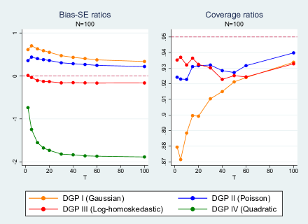
Figure 2: Simulated bias/SE and coverage ratios for three-way FE-PPML estimates as the time dimension ($T$) becomes increasingly large. The data is generated in the same way as in Tables 1-3. The $i$ and $j$ dimensions are fixed at $N=100$. The values for $T$ are 2, 5, 10, 15, 20, 30, 40, 50, 60, and 100. Coverage for DGP IV (not shown) ranges between 0.52 and 0.84 and generally gets progressively worse at higher values of $T$.

What happens for larger values of $T$?

Based on our Remark 2, one might expect that increasing the size of the time dimension should reduce the asymptotic bias in relation to the standard error. However, in the range of $T$ values we used in Tables 1-3, this is not what we observe. The question thus arises: can we say if there exists a “large enough” value of $T$ beyond which researchers may feel relatively secure about IPPs?

Figure 2 addresses this question by presenting simulated bias/SE and coverage ratios for a wider range of $T$ values, spanning from $2$ to $100$. $N$ is fixed at 100, and the data is otherwise generated the same way as before. If we focus just on the first two DGPs, the Gaussian and Poisson cases, we do indeed observe steady improvements in both ratios as $T$ increases, though coverage fails to hit $0.95$ in either case. However, for both DGP III (log-homoskedastic) and DGP IV (quadratic), we actually observe bias/SE ratios getting worse as $T$ approaches 100. In the case of DGP IV, coverage actually gets worse as well. The main takeaway is that gravity panels with seemingly large time spans are not necessarily immune to IPPs. To reconcile these findings with our theory, note that Remark 2 only says that three-way PPML estimates become asymptotically unbiased as both $N$ and $T$ become large simultaneously. In further simulations, we have confirmed that both the bias/SE ratio and coverage improve across all DGPs when we compare, e.g., $N=T=200$ with $N=T=100.$

5 Empirical Applications

For our main empirical application, we estimate the average effects of an FTA for a variety of different industries using a panel with a relatively large number of countries. The value of this exercise is that we expect that trade flows could be distributed very differently across different industries. Based on our results so far, this should lead to a range of differerent bias behaviors in the data.

Our trade data is from the BACI database of Gaulier and Zignago (2010), from which we extract data on trade flows between 167 countries for the years 1995, 2000, 2005, 2010, and 2015. Countries are chosen so that the same 167 countries always appear as both exporters and importers in every period; hence, the data readily maps to the setting just described with $N=167$ and $T=5$. We combine this trade data with data on FTAs from the NSF-Kellogg database maintained by Scott Baier and Jeff Bergstrand, which we crosscheck against data from the WTO in order to incorporate agreements from more recent years. The specification we estimate is

$$y_{ijt} =\exp[\alpha_{it}+\gamma_{jt}+\eta_{ij}+\beta FTA_{ijt}]\omega_{ijt},$$ (15)

where $y_{ijt}$ is trade flows (measured in current USD), $FTA_{ijt}$ is a $0/1$ dummy for whether or not $i$ and $j$ have an FTA at time $t$, and $\omega_{ijt}$ is an error term. As we have noted, estimation of specifications such as (15) via PPML has become an increasingly standard method for estimating the effects of FTAs and other trade policies and is currently recommended as such by the WTO (see Yotov, Piermartini, Monteiro, and Larch, 2016.)

Table 4 presents results from FE-PPML estimation of (15), including results obtained using our bias corrections. The estimation is applied separately to 28 2 digit ISIC (rev. 3) industries as well as to aggregate trade. While we do indeed see a range of different biases in the industry-level estimates, the results for aggregate trade flows, shown in the bottom row of Table 4, are fairly representative. To provide some basic interpretation, the coefficient on $FTA_{ijt}$ for aggregate trade is initially estimated to be $0.082$, which equates to an $e^{0.082}-1=8.5\%$ average “partial” effect of an FTA on trade. The estimated standard error is $0.027$, implying that this effect is statistically different from zero at the $p<0.01$ significance level. Our bias-corrected estimates do not paint an altogether different picture, but do highlight the potential for meaningful refinement. Both the analytical and jackknife bias corrections for $\beta$ suggest a downward bias of $0.04$-$0.06$, or about $15\%$-$22\%$ of the estimated standard error. As our bias-corrected standard errors show (in the last column of Table 4), the initially estimated standard error itself has an implied downward bias of $11\%$ (i.e., $0.027$ versus $0.030$).

Turning to the industry-level estimates, the analytical bias correction more often than not indicates a downward bias ranging between $5\%$-$20\%$ of the estimated standard error, though exceptions are present on both sides of this range. Estimates for the Chemical and Furniture industries appear to be unbiased, for example, and some (such as Tobacco) are associated with an upward bias. On the other end of the spectrum, implied downward biases can also be larger than $20\%$ of the standard error, as is seen for Petroleum ($47\%$), Fabricated Metal Products ($31\%$), Electrical Equipment ($27\%$), and Agriculture ($22\%$). The biases implied by the jackknife are often even larger (see Fabricated Metal Products, for example), consistent with what we found in our simulations for smaller panel sizes. One possible interpretation is that the jackknife-corrected estimates are giving us a less conservative alternative to the analytical corrections in these cases. Indeed, the general correspondence between the two sets of results adds validity to both methods. However, as we have noted, these jackknife estimates could also be reflecting non-homogeneity in the data and/or the higher variance introduced by the jackknife. Implied biases in the standard error, meanwhile, tend to range between $10\%$-$20\%$ of the original standard error, again with some exceptions.

To further illustrate the types of results that can occur, we also obtain replication data for several recent articles that have used three-way gravity models and re-examine their findings using our bias corrections. The results, reported in Table 5, help to demonstrate how these corrections can matter for assessing statistical significance. Instances where conventional significance levels are affected include the coefficients for $\text{EIA}\times\text{CONTIG}$ and $\text{EIA}\times\text{LEGAL}$ from Baier, Bergstrand, and Clance (2018) and the coefficient for log approval rating from Rose (2019). The implied bias to standard error ratios are sometimes as large as 40%-45%, as occurs for the $\text{EIA}\times\text{LANG}$ coefficient from Baier, Bergstrand, and Clance (2018) and the Total EIA Effect from Bergstrand, Larch, and Yotov (2015). However, the largest effects are actually for the standard error, which is downward-biased by more than 40% in several cases (the Total FTA effect from Baier, Yotov, and Zylkin (2019), for example). Notably, there are meaningful differences found even for the data used in Larch, Wanner, Yotov, and Zylkin (2019), a large data set with 213 countries and 66 time periods. These results reinforce our earlier finding that bias corrections may be useful even in settings with seemingly large $N$ and $T$.

6 Conclusion

Thanks to recent methodological and computational advances, nonlinear models with three-way fixed effects have become increasingly popular for investigating the effects of trade policies on trade flows. However, the asymptotic and finite-sample properties of three-way fixed effects estimators have not been rigorously studied, especially with regards to potential IPPs. The performance of the FE-PPML estimator in particular is of natural interest in this context, both because FE-PPML is known to be relatively robust to IPPs as well as because it is likely to be a researcher’s first choice for estimating three-way gravity models. Our results regarding the consistency of PPML in this setting reflect these unique properties of PPML and support its current status as a workhorse estimator for estimating the effects of trade polices.

Given the consistency of PPML in this setting, and given the nice IPP-robustness properties of PPML in general, it may come as a surprise that three-way PPML estimates nonetheless suffer from an asymptotic bias that affects the validity of inferences. In theory, the bias should become less of a problem when the country and time dimensions are both large, but our experiments with the time dimension indicate the bias can be of comparable magnitude to the standard error even in ostensibly large trade data sets. Typical cluster-robust estimates of the standard error are also biased, implying estimated confidence intervals not only off-center but also too narrow.

These issues are not so severe that they leave researchers in the wilderness, but we do recommend taking advantage of the corrective measures we have described. In particular, we find that analytical bias corrections based on Taylor expansions to both the point estimates and standard errors generally lead to improved inferences when applied simultaneously. We caution that we have not found these corrections to be a panacea, however, and several avenues remain open for future work. For example, confidence interval estimates could be adjusted further to account for the uncertainty in the estimated variance—Kauermann and Carroll (2001) describe such a correction for the PPML case. A quasi-differencing approach similar to Jochmans (2016) could provide another angle of attack, and a recent contribution by Pfaffermayr (2021) suggests that jackknife and bootstrap confidence interval methods hold promise as well. Turning to broader applications, the essential dyadic structure of our bias corrections could be easily adapted to network models that study changes in network behavior over time, including settings that involve studying the number of interactions between network members.

Table 1: Finite-sample Properties of Three-way FE-PPML Estimates

				N=20				N=50				N=100
				T=2	T=5	T=10		T=2	T=5	T=10		T=2	T=5	T=10
A. Gaussian DGP (“DGP I”)
Average bias ($\times 100$)
	FE-PPML			6.647	3.764	2.364		2.854	1.497	0.913		1.463	0.755	0.428
	Analytical			2.261	1.005	0.543		0.529	0.165	0.104		0.152	0.043	0.011
	Jackknife			0.558	0.024	-0.304		0.247	0.014	-0.035		0.074	0.006	-0.025
Bias / SE ratio
	FE-PPML			0.690	0.796	0.753		0.668	0.732	0.687		0.644	0.708	0.626
	Analytical			0.235	0.213	0.173		0.124	0.081	0.078		0.067	0.040	0.016
	Jackknife			0.058	0.005	-0.097		0.058	0.007	-0.026		0.033	0.006	-0.037
SE / SD ratio
	FE-PPML			0.836	0.846	0.868		0.901	0.916	0.936		0.934	0.949	0.968
	Analytical			0.792	0.813	0.845		0.859	0.887	0.921		0.899	0.929	0.958
	Jackknife			0.718	0.752	0.783		0.831	0.863	0.900		0.887	0.918	0.949
Coverage probability (should be $0.95$ for an unbiased estimator)
	FE-PPML			0.836	0.804	0.823		0.856	0.846	0.870		0.874	0.870	0.889
	Analytical			0.871	0.883	0.895		0.907	0.921	0.930		0.922	0.933	0.941
	Jackknife			0.841	0.866	0.876		0.901	0.911	0.926		0.916	0.929	0.939
B. Poisson DGP (“DGP II”)
Average bias ($\times 100$)
	FE-PPML			3.840	2.161	1.358		1.621	0.857	0.541		0.825	0.435	0.249
	Analytical			1.193	0.621	0.421		0.237	0.095	0.094		0.063	0.024	0.010
	Jackknife			0.229	0.002	-0.153		0.079	0.007	0.001		0.018	0.004	-0.013
Bias / SE ratio
	FE-PPML			0.403	0.466	0.446		0.394	0.439	0.430		0.386	0.436	0.390
	Analytical			0.125	0.134	0.138		0.058	0.049	0.075		0.029	0.024	0.016
	Jackknife			0.024	0.000	-0.050		0.019	0.004	0.001		0.008	0.004	-0.020
SE / SD ratio
	FE-PPML			0.865	0.869	0.891		0.931	0.940	0.957		0.957	0.965	0.982
	Analytical			0.824	0.838	0.869		0.903	0.924	0.947		0.939	0.957	0.977
	Jackknife			0.748	0.774	0.804		0.875	0.898	0.924		0.926	0.942	0.966
Coverage probability (should be $0.95$ for an unbiased estimator)
	FE-PPML			0.887	0.880	0.892		0.912	0.905	0.919		0.918	0.919	0.925
	Analytical			0.888	0.897	0.902		0.920	0.931	0.938		0.934	0.939	0.948
	Jackknife			0.857	0.870	0.884		0.916	0.922	0.934		0.928	0.936	0.945
Notes: Results computed using 5,000 repetitions. The model being estimated is $y_{ijt}=\lambda_{ijt}\omega_{ijt}$, where $\lambda_{ijt}=\exp(\alpha_{it}+\gamma_{jt}+\eta_{ij}+\beta x_{ijt})$. The data is generated using $\alpha_{it}\sim\mathcal{N}(0,1/16)$, $\gamma_{jt}\sim\mathcal{N}(0,1/16)$, $\eta_{ij}\sim\mathcal{N}(0,1/16)$ and $\beta=1$. $x_{ijt}=x_{ijt-1}/2+\alpha_{it}+\gamma_{jt}+\eta_{ij}+\nu_{ijt}$, with $x_{ij0}=\eta_{ij}+\nu_{ij0}$ and $\nu_{ijt}\sim\mathcal{N}(0,1/2)$. Results are shown for two different assumptions about $V(y_{ijt})$. The “Gaussian” DGP (panel A) assumes $V(\omega_{ijt})=\lambda_{ijt}^{-2}$. The “Poisson” DGP (panel B) assumes $V(\omega_{ijt})=\lambda_{ijt}^{-1}$.SE/SD refers to the ratio of the average standard error of of $\widehat{\beta}$ relative to the standard deviation of $\widehat{\beta}$ across simulations. Coverage probability refers to the probability $\beta^{0}$ is covered in the 95% confidence interval for $\widehat{\beta}_{NT}$. “Analytical” and “Jackknife” respectively indicate Analytical and Jackknife bias-corrected FE-PPML estimates. “FE-PPML” indicates uncorrected estimates. SEs allow for within-$ij$ clustering.

Table 2: Finite-sample Properties of Three-way FE-PPML Estimates

				N=20				N=50				N=100
				T=2	T=5	T=10		T=2	T=5	T=10		T=2	T=5	T=10
A. Log-homoskedastic DGP (“DGP III”)
Average bias ($\times 100$)
	FE-PPML			0.368	-0.086	-0.248		0.143	-0.092	-0.119		0.083	-0.051	-0.088
	Analytical			-0.103	-0.108	-0.048		-0.065	-0.073	-0.004		-0.012	-0.024	-0.016
	Jackknife			-0.189	-0.286	-0.302		-0.064	-0.077	-0.038		-0.012	-0.021	-0.023
Bias / SE ratio
	FE-PPML			0.036	-0.017	-0.074		0.032	-0.042	-0.081		0.036	-0.044	-0.114
	Analytical			-0.010	-0.021	-0.014		-0.015	-0.033	-0.003		-0.005	-0.021	-0.021
	Jackknife			-0.019	-0.057	-0.090		-0.014	-0.035	-0.026		-0.005	-0.018	-0.030
SE / SD ratio
	FE-PPML			0.853	0.838	0.848		0.920	0.910	0.923		0.949	0.943	0.956
	Analytical			0.801	0.787	0.799		0.881	0.874	0.885		0.922	0.918	0.930
	Jackknife			0.727	0.726	0.744		0.853	0.850	0.863		0.908	0.902	0.920
Coverage probability (should be $0.95$ for an unbiased estimator)
	FE-PPML			0.903	0.898	0.899		0.933	0.927	0.923		0.937	0.936	0.940
	Analytical			0.884	0.874	0.882		0.919	0.917	0.914		0.931	0.929	0.934
	Jackknife			0.846	0.843	0.852		0.912	0.907	0.902		0.924	0.923	0.935
B. Quadratic DGP (“DGP IV”)
Average bias ($\times 100$)
	FE-PPML			-6.136	-5.658	-5.098		-3.560	-3.348	-2.935		-2.207	-2.114	-1.878
	Analytical			-4.592	-3.983	-3.415		-2.088	-1.907	-1.588		-1.021	-0.990	-0.857
	Jackknife			-3.752	-3.517	-3.116		-1.794	-1.674	-1.414		-0.922	-0.893	-0.774
Bias / SE ratio
	FE-PPML			-0.510	-0.898	-1.171		-0.640	-1.114	-1.384		-0.718	-1.242	-1.544
	Analytical			-0.382	-0.632	-0.784		-0.375	-0.634	-0.749		-0.332	-0.582	-0.704
	Jackknife			-0.312	-0.558	-0.716		-0.323	-0.557	-0.667		-0.300	-0.525	-0.636
SE / SD ratio
	FE-PPML			0.799	0.759	0.749		0.847	0.809	0.809		0.877	0.844	0.844
	Analytical			0.734	0.693	0.682		0.781	0.738	0.734		0.811	0.773	0.770
	Jackknife			0.662	0.635	0.633		0.747	0.710	0.707		0.795	0.756	0.755
Coverage probability (should be $0.95$ for an unbiased estimator)
	FE-PPML			0.849	0.760	0.700		0.844	0.734	0.673		0.848	0.705	0.619
	Analytical			0.830	0.775	0.749		0.849	0.799	0.780		0.871	0.823	0.801
	Jackknife			0.795	0.749	0.729		0.840	0.795	0.786		0.867	0.818	0.803
Notes: Results computed using 5,000 repetitions. The model being estimated is $y_{ijt}=\lambda_{ijt}\omega_{ijt}$, where $\lambda_{ijt}=\exp(\alpha_{it}+\gamma_{jt}+\eta_{ij}+\beta x_{ijt})$. The data is generated using $\alpha_{it}\sim\mathcal{N}(0,1/16)$, $\gamma_{jt}\sim\mathcal{N}(0,1/16)$, $\eta_{ij}\sim\mathcal{N}(0,1/16)$ and $\beta=1$. $x_{ijt}=x_{ijt-1}/2+\alpha_{it}+\gamma_{jt}+\eta_{ij}+\nu_{ijt}$, with $x_{ij0}=\eta_{ij}+\nu_{ij0}$ and $\nu_{ijt}\sim\mathcal{N}(0,1/2)$. Results are shown for two different assumptions about $V(y_{ijt})$. The “Log-homoskedastic” DGP (panel A) assumes $V(y_{ijt})=\lambda_{ijt}^{2}$. The “Quadratic” DGP (Panel D) assumes $\omega_{ijt}$ is log-normal with variance equal to $\lambda_{ijt}^{-1}+\exp(2x_{ijt})$. SE/SD refers to the ratio of the average standard error of of $\widehat{\beta}$ relative to the standard deviation of $\widehat{\beta}$ across simulations. Coverage probability refers to the probability $\beta^{0}$ is covered in the 95% confidence interval for $\widehat{\beta}_{NT}$. “Analytical” and “Jackknife” respectively indicate Analytical and Jackknife bias-corrected FE-PPML estimates. “FE-PPML” indicates uncorrected estimates. SEs allow for within-$ij$ clustering.

Table 3: Improving Coverage in Three-way FE-PPML Gravity Estimates

				N=20				N=50				N=100
				T=2	T=5	T=10		T=2	T=5	T=10		T=2	T=5	T=10
A. Gaussian DGP (“DGP I”)
SE / SD ratio with corrected SEs
	FE-PPML			0.936	0.930	0.946		0.953	0.957	0.971		0.965	0.972	0.988
	Analytical			0.887	0.894	0.921		0.908	0.927	0.956		0.929	0.952	0.978
	Jackknife			0.803	0.827	0.854		0.879	0.902	0.935		0.917	0.941	0.968
Coverage probability with corrected SEs (should be $0.95$ for an unbiased estimator)
	(uncorrected)			0.836	0.804	0.823		0.856	0.846	0.870		0.874	0.870	0.889
	FE-PPML			0.877	0.846	0.856		0.881	0.866	0.885		0.889	0.877	0.895
	Analytical			0.909	0.912	0.918		0.925	0.930	0.941		0.931	0.940	0.948
	Jackknife			0.884	0.901	0.908		0.920	0.923	0.938		0.926	0.935	0.944
B. Poisson DGP (“DGP II”)
SE / SD ratio with corrected SEs
	FE-PPML			0.966	0.956	0.974		0.979	0.980	0.993		0.983	0.986	1.001
	Analytical			0.920	0.922	0.950		0.949	0.963	0.983		0.964	0.978	0.996
	Jackknife			0.834	0.851	0.879		0.920	0.936	0.960		0.951	0.962	0.985
Coverage probability with corrected SEs (should be $0.95$ for an unbiased estimator)
	(uncorrected)			0.887	0.880	0.892		0.912	0.905	0.919		0.918	0.919	0.925
	FE-PPML			0.923	0.915	0.916		0.927	0.921	0.930		0.925	0.927	0.931
	Analytical			0.923	0.929	0.930		0.938	0.942	0.949		0.942	0.945	0.952
	Jackknife			0.900	0.903	0.915		0.932	0.935	0.942		0.936	0.941	0.949
C. Log-homoskedastic DGP (“DGP III”)
SE / SD ratio with corrected SEs
	FE-PPML			0.966	0.943	0.954		0.979	0.967	0.979		0.984	0.976	0.989
	Analytical			0.906	0.886	0.899		0.938	0.928	0.940		0.956	0.951	0.962
	Jackknife			0.823	0.817	0.837		0.908	0.902	0.916		0.942	0.934	0.952
Coverage probability with corrected SEs (should be $0.95$ for an unbiased estimator)
	(uncorrected)			0.903	0.898	0.899		0.933	0.927	0.923		0.937	0.936	0.940
	FE-PPML			0.938	0.934	0.932		0.947	0.942	0.940		0.945	0.943	0.949
	Analytical			0.922	0.914	0.915		0.938	0.932	0.929		0.940	0.939	0.943
	Jackknife			0.892	0.889	0.899		0.930	0.925	0.924		0.935	0.934	0.942
D. Quadratic DGP (“DGP IV”)
SE / SD ratio with corrected SEs
	FE-PPML			0.952	0.861	0.929		0.947	0.948	0.949		0.970	0.924	0.882
	Analytical			0.877	0.793	0.845		0.873	0.865	0.865		0.897	0.853	0.810
	Jackknife			0.781	0.729	0.786		0.833	0.824	0.837		0.889	0.828	0.789
Coverage probability with corrected SEs (should be $0.95$ for an unbiased estimator)
	(uncorrected)			0.849	0.760	0.700		0.844	0.734	0.673		0.848	0.705	0.619
	FE-PPML			0.900	0.820	0.808		0.894	0.806	0.762		0.892	0.752	0.652
	Analytical			0.894	0.830	0.838		0.908	0.864	0.862		0.918	0.856	0.818
	Jackknife			0.844	0.808	0.814		0.894	0.860	0.866		0.908	0.848	0.822
Notes: Results computed using 5,000 repetitions. The data is generated in the same manner as Tables 1 and 2 SE/SD refers to the ratio of the average standard error of $\widehat{\beta}$ relative to the standard deviation of $\widehat{\beta}$ across simulations. Coverage probability refers to the probability $\beta^{0}$ is covered in the 95% confidence interval for $\widehat{\beta}$. “Analytical” and “Jackknife” respectively indicate Analytical and Jackknife bias-corrected FE-PPML estimates. “FE-PPML” estimates use corrections for the SEs only. SEs allow for within-$ij$ clustering. The corrected SEs correct for first-order finite sample bias in the estimated variance.

Table 4: Bias Correction Results Using BACI Trade Data ($N=167$)

			Original estimates			Bias-corrected estimates
Industry	Code		$\widehat{\beta}$	SE		Analytical	Jackknife	SE
Agriculture	1		0.097	(0.046)		0.107	0.109	(0.051)
Forestry	2		-0.203	(0.125)		-0.197	-0.185	(0.156)
Fishing	5		0.127	(0.141)		0.140	0.189	(0.164)
Coal	10		0.025	(0.131)		0.011	-0.079	(0.163)
Metal Ores	13		0.040	(0.100)		0.032	-0.020	(0.124)
Other Mining & Quarrying n.e.c.	14		0.048	(0.097)		0.079	0.098	(0.108)
Food & Beverages	15		0.020	(0.043)		0.027	0.029	(0.048)
Tobacco	16		0.535	(0.139)		0.525	0.598	(0.163)
Textiles	17		0.229	(0.045)		0.227	0.238	(0.055)
Apparel	18		0.092	(0.092)		0.094	0.132	(0.120)
Leather Products	19		0.222	(0.067)		0.218	0.242	(0.079)
Wood & Cork Products	20		0.077	(0.109)		0.098	0.102	(0.127)
Paper & Paper Products	21		-0.002	(0.062)		-0.004	-0.018	(0.071)
Printed & Recorded Media	22		-0.114	(0.065)		-0.144	-0.177	(0.076)
Coke & Refined Petroleum	23		0.254	(0.076)		0.290	0.340	(0.090)
Chemicals & Chemical Products	24		0.072	(0.035)		0.072	0.077	(0.040)
Rubber & Plastic Products	25		0.141	(0.030)		0.146	0.154	(0.035)
Non-metallic Mineral Products	26		0.218	(0.049)		0.225	0.232	(0.058)
Basic Metal Products	27		0.267	(0.102)		0.272	0.302	(0.115)
Fabricated Metal Products (excl. Machinery)	28		0.196	(0.036)		0.207	0.226	(0.041)
Machinery & Equipment n.e.c.	29		0.049	(0.036)		0.052	0.055	(0.041)
Office, Accounting, and Computer Equipment	30		-0.036	(0.062)		-0.044	-0.038	(0.074)
Electrical Equipment	31		0.214	(0.045)		0.226	0.240	(0.052)
Communications Equipment	32		-0.127	(0.067)		-0.143	-0.174	(0.081)
Medical & Scientific Equipment	33		0.062	(0.039)		0.069	0.087	(0.044)
Motor Vehicles, Trailers & Semi-trailers	34		0.158	(0.064)		0.170	0.196	(0.077)
Other Transport Equipment	35		0.207	(0.124)		0.230	0.251	(0.137)
Furniture & Other Manufacturing n.e.c.	36		0.225	(0.073)		0.225	0.228	(0.082)
Total	All		0.082	(0.027)		0.086	0.088	(0.030)
Notes: These results are computed using ISIC Rev. 3 industry-level trade data for trade between 167 countries during years 1995, 2000, 2005, 2010, & 2015. The original data is from BACI. The model being estimated is $y_{ijt}=\exp(\alpha_{it}+\gamma_{jt}+\eta_{ij}+\beta FTA_{ijt})\omega_{ijt}$, where $y_{ijt}$ is the trade volume and $FTA_{ijt}$ is a dummy for the presence of an FTA. $\alpha_{it}$, $\gamma_{jt}$, & $\eta_{ij}$ respectively denote exporter-time, importer-time, & exporter-importer fixed effects. We estimate each industry separately. The jackknife corrections use the average of 200 randomly-assigned split-panel partitions. SEs are clustered by exporter-importer.

Table 5: Further Applications

Article	Covariate	original PPML coefficient and standard error	bias-corrected estimate	Notes
Baier, Bergstrand, and Clance (2018)	EIA	0.062 (0.039)	0.073 (0.044)*	EIA is a dummy for the presence of an Economic Integration Agreement. The interaction terms are log distance and dummies for adjacency, common legal system, common religion, common language, and colonial history. Our estimation differs from BBF’s in that we use PPML, whereas BBF use OLS with first-differences and pair-specific time trends. The specification we replicate is their Table 4, column 7. 183 countries, 1965-2010 every 5 years ($N=183,$ $T=10$).
	EIA $\times$ log DIST	-0.102 (0.031)***	-0.094 (0.035)***
	EIA $\times$ CONTIG	-0.250 (0.096)***	-0.266 (0.140)*
	EIA $\times$ LEGAL	0.160 (0.078)**	0.189 (0.111)*
	EIA $\times$ RELG	0.418 (0.125)***	0.456 (0.166)***
	EIA $\times$ LANG	-0.414 (0.103)***	-0.457 (0.147)***
	EIA $\times$ CLNY	-0.082 (0.116)	-0.051 (0.147)
Baier, Bergstrand, and Feng (2014)	Total NRPTA Effect	0.020 (0.091)	0.035 (0.110)	NRPTA is a non-reciprocal trade preference. PTA is a reciprocal preferential trade agreement. FTA is a free trade agreement with additional provisions beyond tariff reductions. CUCMECU refers to customs unions, monetary unions, and economic unions. “Total” effects are inclusive of 5 year lags. Our estimation differs from BBF’s in that we use PPML, whereas BBF use OLS with first-differences and pair-specific time trends. The specification we replicate is their Table 1, Column 2a. 149 countries, 1965-2000 ($N=149,$ $T=8$).
	Total PTA Effect	0.149 (0.079)*	0.160 (0.089)*
	Total FTA Effect	0.365 (0.045)***	0.352 (0.061)***
	Total CUCMECU Effect	0.670 (0.060)***	0.669 (0.070)***
Baier, Yotov, and Zylkin (2019)	Total FTA Effect	0.292 (0.051)***	0.299 (0.074)***	Reported coefficient is for the “Total FTA effect” inclusive of 5-year lags. The specification we estimate is their equation (4). Our estimate differs slightly because we use asymmetric pair fixed effects instead of symmetric pair fixed effects. Our standard errors differ because we cluster by pair. 69 countries, 1986-2006 ($N=69$, $T=21$).
Bergstrand, Larch, and Yotov (2015)	Total EIA Effect	0.521 (0.060)***	0.546 (0.098)***	Reported coefficient is for the “Total EIA effect” inclusive of 4- and 8-year lags for the same specification as in their Table 2, column 4. Baseline estimates differ slightly because BLY originally used symmetric pair fixed effects whereas we use asymmetric pair fixed effects. 41 countries, 1990-2002, every 4 years ($N=41$, $T=4$).
Larch, Wanner, Yotov, and Zylkin (2019)	Euro	0.030 (0.042)	0.021 (0.046)	The specification we replicate is their Table 1, column 5, which in turn replicates the main specification from Glick and Rose (2016). Our standard errors differ because we cluster by pair. 213 countries, 1948-2013 ($N=213$, $T=66$).
	Other CUs	0.700 (0.107)***	0.708 (0.142)***
	RTA	0.169 (0.040)***	0.159 (0.050)***
	Curr. Colony	0.545 (0.220)**	0.577 (0.262)**
Rose (2019)	log approval rating	0.053 (0.022)***	0.058 (0.028)**	These reported coefficient is from Table 4 of Rose (2019). Log approval rating is a measure of the importing country’s approval of the exporting country’s leader. There are 5 exporters, 149 importers, and 12 years (2006-2017).
This table shows replications of several recent papers that use three-way gravity models with exporter-time, importer-time, and country-pair fixed effects. Standard errors shown in parentheses. Bias-corrected estimates use our analytical corrections for the point estimates and standard errors. * $p<0.10$ , ** $p<.05$ , *** $p<.01$.

Appendix A Appendix

This Appendix first describes an additional simulation exercise based on the trade data. We then introduce additional notation, definitions, and other technical details that supplement the formal theorems and remarks presented in Section 3. Proofs of our formal results then follow, starting with a poof of Proposition 3, which characterizes the asymptotic distribution of $\widehat{\beta}$ and its asymptotic bias. This proof naturally lends itself to further discussion of the “large $T$” results from Remark 2 as well as the consistency result from Proposition 15, which itself follows as a by-product of Proposition 3. We then demonstrate the uniqueness of this latter result as stated in Proposition 2 and highlight the general inconsistency of other three-way gravity estimators.

After the proofs, we include further supplementary discussions on the downward bias in the estimated standard errors, on allowing for conditional dependence across pairs in the trade data, and on how FE-PPML is affected by IPPs in more general settings beyond the gravity framework.

A.1 Simulation Based on Trade Data

As a additional simulation exercise, we revisit the BACI aggregate trade data we used in Section 5 and ask: if the estimated effect of an FTA and its standard error were indeed biased to the degrees implied by our bias corrections, would our corrections be successful at correctly identifying the bias and improving inference?

To answer this question, we start from the original aggregate trade data and FTA data but reconstruct the conditional mean $\lambda_{ijt}$ as though $\beta=0.086$. That is, we first adjust the estimated $\widehat{\lambda}_{ijt}$’s from the original estimation to account for the change in $\beta$ and so that the FOC’s for all fixed effects are consistent with $\beta=0.086$. This gives us new “true” values of the conditional mean that we denote by $\lambda_{ijt}^{(1)}$. The original data is therefore assumed to have been generated by $y_{ijt}=\lambda_{ijt}^{(1)}\omega_{ijt}$, where the true disturbance $\omega_{ijt}$ is backed out using $\omega_{ijt}=y_{ijt}/\lambda_{ijt}^{(1)}$.

Next, we choose a DGP for $\omega_{ijt}$ that can reproduce the biases implied by our corrections. Taking our cues from DGP IV, which we found earlier to produce a downward bias in $\widehat{\beta}$, we consider a DGP where the conditional variance of $y_{ijt}$ has the form $\text{Var}[y_{ijt}|.]=a\lambda_{ijt}+bFTA\lambda_{ijt}^{2}$. That is, we allow for some overdispersion that depends on the regressor of interest, as in DGP IV. We choose the two parameters $a$ and $b$ in order to come close to matching the following three values: (i) the bias in $\widehat{\beta}$, (ii) the standard deviation of $\widehat{\beta}$ (assumed to be $0.03)$, (iii) the bias of the standard error of $\widehat{\beta}$. To keep things simple, all of our simulations sample new values for $\omega_{ijt}$ only, holding $\lambda_{ijt}^{(1)}$ fixed. As in the main text, we use 5,000 replications and assume $\rho=0.3$. For our chosen values of $a$ and $b$—$a=200,000$, $b=0.08$—we obtain an average $\widehat{\beta}$ of $0.0823$, an average standard error of $0.0267$, and a standard deviation of $0.0307$. The uncorrected coverage is $0.9078$.

When our preferred bias corrections are applied, they do not completely solve the coverage problem but do induce across-the-board improvements. The average corrected $\widehat{\beta}$ using the analytical bias correction is $0.0842$ and the corrected standard error is $0.0290$. Coverage improves as well, but only to $0.9210$. As discussed in the main text, one important factor that limits the improvement in coverage is the fact that applying bias corrections to the point estimates increases their variance. In this case, the standard deviation of the corrected estimate is $0.0321$.

Turning to the jackknife bias correction, we find as before that it does a superior job of bias reduction than the analytical correction, producing a average corrected estimate of $0.0851$. However, the standard deviation of the jackknife-corrected estimates is $0.0371$, echoing our previous finding that the improved bias reduction performance of the jackknife comes at a steep penalty in terms of increased variance. As a result, the coverage we obtain when we combine the jackknife with the corrected standard errors is only $0.8756$.

Interestingly, if we only use the correction to the standard errors, i.e., without applying any correction to the point estimates, we obtain a coverage ratio of $0.9312$, which is better than if we also use the analytical correction. It nonetheless remains true that using corrections to both the point estimates and standard errors leads to an improvement in coverage, as we have consistently found throughout our results. In general, these simulations reinforce our earlier conclusion that bias corrections, though helpful, are not necessarily a panacea to the issues we raise in the paper.

A.2 Additional Notation and Definitions

It is convenient to define the log-likelihood as a function of the index vector $\pi_{ij}$ as follows,

$$\ell_{ij}(\beta,\alpha_{i},\gamma_{j}) =:\ell_{ij}(\beta,\pi_{ij}), \pi_{ij}=\left(\begin{array}[]{c}\pi_{ij1}\\ \vdots\\ \pi_{ijT}\end{array}\right):=\left(\begin{array}[]{c}\alpha_{i1}+\gamma_{j1}\\ \vdots\\ \alpha_{iT}+\gamma_{jT}\end{array}\right).$$ where

In this appendix, we will also be more explicit than in the main text in distinguishing true parameter values $\beta^{0}$, $\alpha^{0}_{it}$, $\gamma_{jt}^{0}$, and the corresponding $\pi_{ij}^{0}$ and $\vartheta^{0}_{ijt}$, from their generic equivalents. For example, the $S_{ij}$, $H_{ij}$ and $G_{ij}$ that were already defined in the main text can more formally be written as

$$S_{ij} :=-\frac{\partial^{2}\ell_{ij}(\beta^{0},\pi^{0}_{ij})}{\partial\pi_{ij}}, H_{ij} :=-\frac{\partial^{2}\ell_{ij}(\beta^{0},\pi^{0}_{ij})}{\partial\pi_{ij}\,\partial\pi_{ij}^{\prime}},$$

and

$$G_{ij,tsr} =\frac{\partial^{3}\ell_{ij}(\beta^{0},\pi^{0}_{ij})}{\partial\pi_{ijt}\,\partial\pi_{ijs}\,\partial\pi_{ijr}}=\left\{\begin{array}[]{ll}-\vartheta^{0}_{ijt}\left(1-\vartheta^{0}_{ijt}\right)\left(1-2\vartheta^{0}_{ijt}\right)\sum_{\tau}y_{ij\tau}&\text{if $t=s=r$,}\\ -\vartheta^{0}_{ijs}\left(1-2\vartheta^{0}_{ijs}\right)\vartheta^{0}_{ijt}\sum_{\tau}y_{ij\tau}&\text{if $s=r\neq t$,}\\ -\vartheta^{0}_{ijs}\left(1-2\vartheta^{0}_{ijs}\right)\vartheta^{0}_{ijr}\sum_{\tau}y_{ij\tau}&\text{if $t=s\neq r$,}\\ -\vartheta^{0}_{ijt}\left(1-2\vartheta^{0}_{ijt}\right)\vartheta^{0}_{ijs}\sum_{\tau}y_{ij\tau}&\text{if $r=t\neq s$,}\\ -2\vartheta^{0}_{ijr}\vartheta^{0}_{ijs}\vartheta^{0}_{ijt}\sum_{\tau}y_{ij\tau}&\text{if $r\neq s\neq t\neq r$.}\end{array}\right.$$

The $T\times K$ matrix $\widetilde{x}_{ij}$ that was informally introduced in the main text as a two-way within-transformation of $x_{ij}$, can be formally defined by $\widetilde{x}_{ij}=x_{ij}-\alpha_{i}^{x}-\gamma_{j}^{x}$, where $\alpha_{i}^{x}$ and $\gamma_{j}^{x}$ are $T\times K$ matrices that minimize

$${\sum_{i=1}^{N}\sum_{j\in\mathfrak{N}\setminus\{i\}}}{\rm Tr}\left[\left(x_{ij}-\alpha_{i}^{x}-\gamma_{j}^{x}\right)^{\prime}\,\bar{H}_{ij}\,\left(x_{ij}-\alpha_{i}^{x}-\gamma_{j}^{x}\right)\right],$$ (16)

subject to appropriate normalizations on $\alpha_{i}^{x}$ and $\gamma_{j}^{x}$ (e.g. $\iota_{T}^{\prime}\alpha_{i}^{x}=\iota_{T}^{\prime}\gamma_{j}^{x}=0$, where $\iota_{T}=(1,\ldots,1)^{\prime}$ is a T-vector of ones). Each within-transformed regressor vector $\widetilde{x}_{ij,k}$ can be interpreted as containing the residuals left after partialing out $x_{ij,k}$ with respect to any $i$- and $j$-specific components and weighting by $\bar{H}_{ij}$.

A.2.1 Analytical Bias Correction Formulas

The analytical bias correction discussed in Section 3.4 of the main text requires estimates of the expressions $W_{N}$, $B_{N}$, $D_{N}$ defined in Proposition 3. For this, we first require plugin objects $\widehat{\widetilde{x}}_{ij}$, $\widehat{S}_{ij}$, $\widehat{H}_{ij}$, $\widehat{\overline{H}}_{ij}$, and $\widehat{G}_{ij}$ — these objects are formed in the obvious way by replacing $\lambda_{ijt}$ with $\widehat{\lambda}_{ijt}$ and $\vartheta_{ijt}$ with $\widehat{\vartheta}_{ijt}:=\widehat{\lambda}_{ijt}/\sum_{\tau}\widehat{\lambda}_{ij\tau}$ where needed. Then, the $\widehat{B}_{N}$ and $\widehat{D}_{N}$ are $K$-vectors with elements given by

$$\widehat{B}_{N}^{k} =-\frac{1}{N-1}\sum_{i=1}^{N}\mathrm{Tr}\left[\left(\sum_{j\in\mathfrak{N}\setminus\{i\}}\widehat{\overline{H}}_{ij}\right)^{\dagger}\sum_{j\in\mathfrak{N}\setminus\{i\}}\widehat{H}_{ij}\,\widehat{\widetilde{x}}_{ij,k}\,\widehat{S}_{ij}^{\prime}\right]$$

$$+\frac{1}{2\left(N-1\right)}\sum_{i=1}^{N}\mathrm{Tr}\left[\left(\sum_{j\in\mathfrak{N}\setminus\{i\}}\widehat{G}_{ij}\,\widehat{\widetilde{x}}_{ij,k}\right)\left(\sum_{j\in\mathfrak{N}\setminus\{i\}}\widehat{\overline{H}}_{ij}\right)^{\dagger}\left[\sum_{j\in\mathfrak{N}\setminus\{i\}}\widehat{S}_{ij}\,\widehat{S}{}_{ij}^{\prime}\right]\left(\sum_{j\in\mathfrak{N}\setminus\{i\}}\widehat{\overline{H}}_{ij}\right)^{\dagger}\right],$$

$$\widehat{D}_{N}^{k} =-\frac{1}{N-1}\sum_{j=1}^{N}\mathrm{Tr}\left[\left(\sum_{i\in\mathfrak{N}\setminus\{j\}}\widehat{\overline{H}}_{ij}\right)^{\dagger}\sum_{i\in\mathfrak{N}\setminus\{j\}}\widehat{H}_{ij}\,\widehat{\widetilde{x}}_{ij,k}\,\widehat{S}_{ij}^{\prime}\right]$$

$$+\frac{1}{2\left(N-1\right)}\sum_{j=1}^{N}\mathrm{Tr}\left[\left(\sum_{i\in\mathfrak{N}\setminus\{j\}}\widehat{G}_{ij}\,\widehat{\widetilde{x}}_{ij,k}\right)\left(\sum_{i\in\mathfrak{N}\setminus\{j\}}\widehat{\overline{H}}_{ij}\right)^{\dagger}\left[\sum_{i\in\mathfrak{N}\setminus\{j\}}\widehat{S}_{ij}\,\widehat{S}{}_{ij}^{\prime}\right]\left(\sum_{i\in\mathfrak{N}\setminus\{j\}}\widehat{\overline{H}}_{ij}\right)^{\dagger}\right],$$

and we have

$$\widehat{W} =\frac{1}{N\,(N-1)}\sum_{i=1}^{N}\sum_{j\in\mathfrak{N}\setminus\{i\}}\widehat{\widetilde{x}}_{ij}^{\prime}\,\widehat{\overline{H}}_{ij}\,\widehat{\widetilde{x}}_{ij},$$

The replacement of $N$ with $N-1$ in $\widehat{B}_{N}^{k}$ and $\widehat{D}_{N}^{k}$ stems from a degrees-of-freedom correction. This correction is needed because creating plug-in values for the $\mathbb{E}\left(S_{ij}^{\prime}H_{ij}\,\big{|}x_{ij,k}\right)$ and $\mathbb{E}\left(S_{ij}\,S{}_{ij}^{\prime}\big{|}x_{ij,k}\right)$ objects that appear in Proposition 3 requires computing terms of the form $\mathbb{E}[y_{ijt}^{2}]$ and $\mathbb{E}[y_{ijs}y_{ijt}]$, as illustrated in Remark 1.

A.2.2 Details on large $T$ bias expansion

We also want to explain the result in Remark 2 of the main text in more detail here by rewriting the bias terms $B_{N}$ and $D_{N}$ to illuminate the role of the time dimension. Using generic definitions for $S_{ij}$, $H_{ij}$, $G_{ij}$, and $\widetilde{x}_{ij}$ (e.g., $S_{ij}:=\partial\ell_{ij}/\partial\pi_{ij}$, $H_{ij}:=\partial^{2}\ell_{ij}/\partial\pi_{ij}\partial\pi_{ij}^{\prime}$, etc.), the formulas for the asymptotic distribution in Proposition 3 apply generally to M-estimators based on concave objective functions $\ell_{ij}(\beta,\alpha_{it},\gamma_{jt})$. Unlike in the two-way FE-PPML case, these formulas do not reduce to zero when we further specialize them to the profiled Poisson pseudo-likelihood in (11), but we still find it instructive to do so (e.g., to discuss the large $T$ limit from Remark 2). For that purpose, we define the $T\times T$ matrix $M_{ij}=\mathbf{I}_{T}-\vartheta_{ij}\iota_{T}^{\prime}$. Furthermore, let $\Lambda_{ij}$ be the $T\times T$ diagonal matrix with diagonal elements $\lambda_{ijt}$, and for $i,j\in\{1,\ldots,N\}$ define the $T\times T$ matrices

$$Q_{i} =\frac{1}{N-1}\left(\sum_{j\in\mathfrak{N}\setminus\{i\}}M_{ij}\,\Lambda_{ij}\,M_{ij}^{\prime}\right)^{\dagger}\left(\sum_{j\in\mathfrak{N}\setminus\{i\}}M_{ij}\,\mathbb{E}(y_{ij}y_{ij}^{\prime})\,M_{ij}^{\prime}\right)\left(\sum_{j\in\mathfrak{N}\setminus\{i\}}M_{ij}\,\Lambda_{ij}\,M_{ij}^{\prime}\right)^{\dagger},$$

$$R_{ij} =\mathbb{E}(y_{ij}y_{ij}^{\prime})\,M_{ij}^{\prime}\left(\frac{1}{N-1}\sum_{j^{\prime}\in\mathfrak{N}\setminus\{i\}}M_{ij}\,\Lambda_{ij}\,M_{ij}^{\prime}\right)^{\dagger}\,\Lambda_{ij}M_{ij}^{\prime}.$$

The bias term $B_{N}=(B_{N}^{k})$ in Proposition 3 can then be expressed as

$$B_{N}^{k} =\frac{1}{N(N-1)}\sum_{i=1}^{N}\sum_{j\in\mathfrak{N}\setminus\{i\}}\left[-\frac{\iota_{T}^{\prime}\,R_{ij}\,\widetilde{x}_{ij,k}}{\iota_{T}^{\prime}\lambda_{ij}}+\frac{\lambda_{ij}^{\prime}\,Q_{i}\,\Lambda_{ij}\,M_{ij}^{\prime}\,\widetilde{x}_{ij,k}}{\iota_{T}^{\prime}\lambda_{ij}}\right],$$ (17)

and an analogous formula for $D_{N}$ follows by interchanging $i$ and $j$ appropriately. As long as there is only weak time dependence between observations the matrix objects $R_{ij}$ and $Q_{i}\Lambda_{ij}M_{ij}^{\prime}$ above are both of order 1 as $T\rightarrow\infty$, such that both terms in brackets in (17) are likewise of order 1. This explains the result stated in Remark 2 of the main text.

A.3 Proof of Proposition 3

Known result for two-way fixed effect panel models

Our proof of Proposition 3 relies on results from Fernández-Val and Weidner (2016) – denoted FW in the following. That paper considers a standard panel setting where individuals $i$ are observed over time periods $t$, and mixing conditions (as opposed to conditional independence assumptions) are imposed across time periods. By contrast, we consider a pseudo-panel setting, where the two panel dimensions are labelled by exporters $i$ and importers $j$, and we impose conditional independence assumptions across both $i$ and $j$ here (see also Dzemski, 2018, who employs those results in a directed network setting where outcomes are binary, and Graham, 2017, for the undirected network case.) Given those differences—and before introducing any further complications—we briefly want to restate the main result in FW for the two-way pseudo-panel case. Outcomes $Y_{ij}$, $i,j=1,\ldots,N$, conditional on all the strictly exogenous regressors $X=(X_{ij})$, fixed effect $N$-vectors $\alpha$ and $\gamma$, and common parameters $\beta$ are assumed to be generated as

$$Y_{ij}\mid X,\alpha,\gamma,\beta\sim f_{Y}(\cdot\mid X_{ij},\alpha_{i},\gamma_{j},\beta),$$

where the conditional distribution $f_{Y}$ is known, up to the unknown parameters $\alpha_{i},\gamma_{j}\in\mathbb{R}$ and $\beta\in\mathbb{R}^{K}$. It is furthermore assumed that $\alpha_{i}$ and $\gamma_{j}$ enter the distribution function only through the single index $\pi_{ij}=\alpha_{i}+\gamma_{j}$; that is, the log-likelihood can be defined by

$$\ell_{ij}(\beta,\,\pi_{ij})=\log f_{Y}(Y_{ij}\mid X_{ij},\alpha_{i},\gamma_{j},\beta).$$

The maximum likelihood estimator for $\beta$ is given by

$$\widehat{\beta} =\operatorname*{argmax}_{\beta\in\mathbb{R}^{K}}\max_{\alpha,\gamma\in\mathbb{R}^{N}}\;{\cal L}(\beta,\alpha,\gamma), {\cal L}(\beta,\alpha,\gamma) =\sum_{i,j}\ell_{ij}(\beta,\,\alpha_{i}+\gamma_{j}).$$

Also, define the $K$-vector $\Xi_{ij}$ with components, $k=1,\ldots,K$,

$$\Xi_{ij,k} =\alpha^{\ast}_{i,k}+\gamma^{\ast}_{j,k}, \left(\alpha^{\ast}_{k},\,\gamma^{\ast}_{k}\right) =\operatorname*{argmin}_{\alpha_{i,k},\gamma_{j,k}}\sum_{i,j}\mathbb{E}(-\partial_{\pi^{2}}\ell_{ij})\left(\frac{\mathbb{E}(\partial_{\beta_{k}\alpha_{i}}\ell_{ij})}{\mathbb{E}(\partial_{\alpha_{i}^{2}}\ell_{ij})}-\alpha_{i,k}-\gamma_{j,k}\right)^{2},$$

where here and in the following all expectations are conditional on regressors $X=(X_{ij})$, and on the parameters $\alpha$, $\gamma$, $\beta$. For $q\in\{0,1,2\}$, the (within-transformation) differentiation operator $\mathcal{D}_{\beta\alpha_{i}^{q}}=\mathcal{D}_{\beta\gamma_{j}^{q}}$ is defined by

$$\mathcal{D}_{\beta\alpha_{i}^{q}}\ell_{ij} =\partial_{\beta\alpha_{i}^{q}}\ell_{ij}-\partial_{\alpha_{i}^{q+1}}\ell_{ij}\,\Xi_{ij}, \mathcal{D}_{\beta\gamma_{j}^{q}}\ell_{ij} =\partial_{\beta\gamma_{j}^{q}}\ell_{ij}-\partial_{\gamma_{j}^{q+1}}\ell_{ij}\,\Xi_{ij}.$$ (18)

Theorem 1.

Assume that

• Conditional on $X$, $\alpha^{0}$, $\gamma^{0}$, $\beta^{0}$ the outcomes $Y_{ij}$ are distributed independently across $i$ and $j$ with

  $$Y_{ij}\mid X,\alpha^{0},\gamma^{0},\beta^{0}\sim\exp[\ell_{ij}(\beta^{0},\pi^{0}_{ij})],$$

  where $\pi^{0}_{ij}=\alpha^{0}_{i}+\gamma^{0}_{j}$.

• The map $(\beta,\pi)\mapsto\ell_{ij}(\beta,\pi)$ is four times continuously differentiable, almost surely. All partial derivatives of $\ell_{ij}(\beta,\pi)$ up to fourth order are bounded in absolute value by a function $m(Y_{it},X_{it})>0$, almost surely, uniformly over a convex compact set ${\cal B}\subset\mathbbm{R}^{\dim\beta+1}$, which contains an $\varepsilon$-neighbourhood of $(\beta^{0},\pi^{0}_{ij})$ for all $i,j,N$, and some $\varepsilon>0$. Furthermore, $\max_{i,j}\mathbb{E}[m(Y_{ij},X_{ij})]^{8+\nu}$ is uniformly bounded over $N$, almost surely, for some $\nu>0$.

• For all $N$, the function $(\beta,\alpha,\gamma)\mapsto\mathcal{L}(\beta,\alpha,\gamma)$ is almost surely strictly concave over $\mathbb{R}^{K+2N}$, apart from one “flat direction” described by the transformation $\alpha_{i}\mapsto\alpha_{i}+c$, $\gamma_{j}\mapsto\gamma_{j}-c$, which leaves $\mathcal{L}(\beta,\alpha,\gamma)$ unchanged for all $c\in\mathbb{R}$. Furthermore, there exist constants $b_{\min}$ and $b_{\max}$ such that for all $(\beta,\pi)\in{\cal B}$, $0<b_{\min}\leq-\mathbb{E}\left[\partial_{\alpha_{i}^{2}}\ell_{ij}(\beta,\pi)\right]\leq b_{\max}$, almost surely, uniformly over $i,j,N$.

In addition, assume that the following limits exist

$$\overline{B} =\lim_{N\rightarrow\infty}\left[-\frac{1}{N}\sum_{i,j}\frac{\mathbb{E}\left(\partial_{\alpha_{i}}\ell_{ij}\mathcal{D}_{\beta\alpha_{i}}\ell_{ij}+\frac{1}{2}\mathcal{D}_{\beta\alpha_{i}^{2}}\ell_{ij}\right)}{\sum_{j^{\prime}}\mathbb{E}\left(\partial_{\alpha_{i}^{2}}\ell_{ij^{\prime}}\right)}\right],$$

$$\overline{D} =\lim_{N\rightarrow\infty}\left[-\frac{1}{N}\sum_{i,j}\frac{\mathbb{E}\left(\partial_{\gamma_{j}}\ell_{ij}\mathcal{D}_{\beta\gamma_{j}}\ell_{ij}+\frac{1}{2}\mathcal{D}_{\beta\gamma_{j}^{2}}\ell_{ij}\right)}{\sum_{i^{\prime}}\mathbb{E}\left(\partial_{\gamma_{j}^{2}}\ell_{i^{\prime}j}\right)}\right],$$

$$\overline{W} =\lim_{N\rightarrow\infty}\left[-\frac{1}{N^{2}}\sum_{i,j}\mathbb{E}\left(\partial_{\beta\beta^{\prime}}\ell_{ij}-\partial_{\alpha_{i}^{2}}\ell_{ij}\Xi_{ij}\Xi^{\prime}_{ij}\right)\right],$$

where expectations are conditional on $X$, $\alpha$, $\gamma$, $\beta$. Finally, assume that $\overline{W}>0$. Then, as $N\rightarrow\infty$, we have

$$N\left(\widehat{\beta}-\beta^{0}\right)\;\to_{d}\;\overline{W}^{-1}\,{\cal N}(\overline{B}+\overline{D},\;\overline{W}),$$

Remarks:

• This is just a reformulation of Theorem 4.1 in FW to the case of pseudo-panels, and the proof is provided in that paper. Since we consider only strictly exogenous regressors, all the analysis is conditional on $X$; and the bias term $\overline{B}$ simplifies here, since conditional on $X$ (and the other parameters), we assume independence across both $i$ and $j$. Thus, no Nickell-type bias (Nickell, 1981; Hahn and Kuersteiner, 2002) appears here, but we still have incidental parameter biases because the model is nonlinear (Neyman and Scott, 1948; Hahn and Newey, 2004).

• In the original version of this theorem, the sums in the definitions of ${\cal L}(\beta,\alpha,\gamma)$, $\overline{B}$, $\overline{D}$, and $\overline{W}$ run over all possible pairs $(i,j)\in\{1,\ldots,N\}^{2}$. However, for the trade application in the current paper we assume we only have observations for $i\neq j$; that is, those sums over $i$ and $j$ only run over the set $\{(i,j)\in\{1,\ldots,N\}^{2}\,:\,i\neq j\}$ of $N(N-1)$ observed country pairs. The sum over $j^{\prime}$ (in $\overline{B}$) then also only runs over $j^{\prime}\neq i$, and the sum over $i^{\prime}$ (in $\overline{D}$) only runs over $i^{\prime}\neq j$. It turns out that those changes make no difference to the proof of the theorem, because the proportion of missing observations for each $i$ and $j$ is asymptotically vanishing. For that reason it also does not matter whether we change the $1/N^{2}$ in $\overline{W}$ to $1/[N(N-1)]$, or whether we change $N\left(\widehat{\beta}-\beta^{0}\right)$ to $\sqrt{N(N-1)}\left(\widehat{\beta}-\beta^{0}\right)$. The same equivalence holds throughout our own results for applications in which researchers wish to use observations for which $i=j$ (simply replace $N-1$ with $N$ where appropriate.) It also does not matter for the proof that the number of exporters and importers is the same, since this is already allowed for in FW’s existing results. If we let $I$ be the number of exporters and $J$ be the number of importers, FW’s results apply so long as $I$ and $J$ grow large at the same rate.

• More generally, careful examination of these proofs and results reveals that all explicit appearances of $N$ and $N-1$ in the definitions of $\overline{W}$, $\overline{B}$, and $\overline{D}$ actually play no role in the fully expressed formula for the asymptotic bias, i.e., $N^{-1}\overline{W}(\overline{B}+\overline{D})$. Thus, there is no need to adjust the terms that explicitly depend on $N$ if some of the data are missing. So long as the missing data occur at random, applying the formulas as written should still generally be expected to deliver an asymptotically valid bias correction. A similar observation applies for missing values in the three-way model. That said, if the missing values occur in such a way that some of the $\alpha_{i}$’s or $\gamma_{j}$’s appear only a small number of times in the data, they will tend to be estimated with a larger degree of estimation noise than the other fixed effects, which could affect the performance of bias corrections based on these formulas in practice.

• The above theorem assumes that the log-likelihood $\ell_{ij}(\beta,\,\alpha_{i}+\gamma_{j})$ for $Y_{ij}\mid X,\alpha,\gamma,\beta$ is correctly specified. This is an unrealistic assumption for the PPML estimators in this paper, where we only want to assume that the score of the pseudo-log-likelihood has zero mean at the true parameters, that is, $\mathbb{E}\big{[}\partial_{\beta}\ell_{ij}(\beta^{0},\,\alpha^{0}_{i}+\gamma^{0}_{j})\mid X_{ij},\alpha^{0}_{i},\gamma^{0}_{j},\beta^{0}\big{]}=0$ and $\mathbb{E}\big{[}\partial_{\alpha_{i}}\ell_{ij}(\beta^{0},\,\alpha^{0}_{i}+\gamma^{0}_{j})\mid X_{ij},\alpha^{0}_{i},\gamma^{0}_{j},\beta^{0}\big{]}=0$ and $\mathbb{E}\big{[}\partial_{\gamma_{j}}\ell_{ij}(\beta^{0},\,\alpha^{0}_{i}+\gamma^{0}_{j})\mid X_{ij},\alpha^{0}_{i},\gamma^{0}_{j},\beta^{0}\big{]}=0$. This extension to “conditional moment models” is discussed in Remark 3 of FW. The statement of the theorem then needs to be changed as follows:

  $$N\left(\widehat{\beta}-\beta^{0}\right)\;\to_{d}\;\overline{W}^{-1}\,{\cal N}(\overline{B}+\overline{D},\;\overline{\Omega}),$$ (19)

  where the definition of $\overline{W}$ is unchanged, but the expression of $\overline{B}=\overline{B}_{1}+\overline{B}_{2}$, $\overline{D}=\overline{D}_{1}+\overline{D}_{2}$ and $\overline{\Omega}$ now read

  $$\overline{B}_{1} =\lim_{N\rightarrow\infty}\left[-\frac{1}{N}\sum_{i,j}\frac{\mathbb{E}\left(\partial_{\alpha_{i}}\ell_{ij}\mathcal{D}_{\beta{\alpha_{i}}}\ell_{ij}\right)}{\sum_{j^{\prime}}\mathbb{E}\left(\partial_{{\alpha_{i}}^{2}}\ell_{ij^{\prime}}\right)}\right],$$

  $$\overline{B}_{2} =\lim_{N\rightarrow\infty}\left[\frac{1}{2}\frac{1}{N}\sum_{i}\frac{\left[\sum_{j}\mathbb{E}(\partial_{{\alpha_{i}}}\ell_{ij})^{2}\right]\sum_{j}\mathbb{E}(\mathcal{D}_{\beta{\alpha_{i}}^{2}}\ell_{ij})}{\left[\sum_{j}\mathbb{E}\left(\partial_{{\alpha_{i}}^{2}}\ell_{ij}\right)\right]^{2}}\right]\;,$$

  $$\overline{D}_{1} =\lim_{N\rightarrow\infty}\left[-\frac{1}{N}\sum_{j}\frac{\sum_{i}\mathbb{E}\left[\partial_{\gamma_{j}}\ell_{ij}\mathcal{D}_{\beta{\gamma_{j}}}\ell_{ij}\right]}{\sum_{i}\mathbb{E}\left(\partial_{{\gamma_{j}}^{2}}\ell_{ij}\right)}\right],$$

  $$\overline{D}_{2} =\lim_{N\rightarrow\infty}\left[\frac{1}{2}\,\frac{1}{N}\sum_{j}\frac{\sum_{i}\left[\mathbb{E}(\partial_{{\gamma_{j}}}\ell_{ij})^{2}\right]\sum_{i}\mathbb{E}(\mathcal{D}_{\beta{\gamma_{j}}^{2}}\ell_{ij})}{\left[\sum_{i}\mathbb{E}\left(\partial_{{\gamma_{j}}^{2}}\ell_{ij}\right)\right]^{2}}\right],$$

  $$\overline{\Omega} =\lim_{N\rightarrow\infty}\left[\frac{1}{N^{2}}\sum_{i,j}\mathbb{E}\left[\mathcal{D}_{\beta}\ell_{ij}(\mathcal{D}_{\beta}\ell_{ij})^{\prime}\right]\right].$$ (20)

  These are the formulas that we have to use as a starting point for the bias results derived in this paper.

Our task in the following is to translate and generalize the conditions, statement, and proof of Theorem 1, as extended in (19) and (20), to the case of the three-way PPML estimator discussed in the main text.

Regularity conditions for Proposition 3

The following regularity conditions are required for the statement of Proposition 3 to hold.

Assumption A.

• Conditional on $x=(x_{ijt})$, $\alpha^{0}=(\alpha^{0}_{it})$, $\gamma^{0}=(\gamma^{0}_{jt})$, $\eta^{0}=(\eta^{0}_{ij})$ and $\beta^{0}$, the outcomes $y_{ij}=(y_{ij,1},\ldots,y_{ij,T})^{\prime}$ are distributed independently across $i$ and $j$, and the conditional mean of $y_{ijt}$ is given by equation (8) for all $i$, $j$, $t$.

• The range of $x_{ijt}$, $\alpha^{0}_{it}$ and $\gamma^{0}_{jt}$ is uniformly bounded, and there exists $\nu>0$ such that $\mathbb{E}(y_{ijt}^{8+\nu}|x_{ijt},\alpha_{it},\gamma_{jt},\eta_{ij})$ is uniformly bounded over $i$, $j$, $t$, $N$.

• $\lim_{N\rightarrow\infty}\,W_{N}>0$, with $W_{N}$ defined in Proposition 3.

Those assumptions are very similar to those in Theorem 1 above: Assumption A(i) is analogous to condition (i) in the theorem, except that we only impose the conditional mean of $y_{ijt}$ to be correctly specified, as already discussed in remark (c) above. Notice also that this assumption requires conditional independence across $i$ and $j$, but we do not have to restrict the dependence of $y_{ijt}$ over $t$ for our results.

We consider the Poisson log-likelihood in this paper, which after profiling out $\eta_{ij}$ gives the pseudo-log-likelihood function $\ell_{ij}(\beta,\alpha_{it},\gamma_{jt})$ defined in equation (11). This log-likelihood is strictly concave and arbitrarily often differentiable in the parameters, so corresponding assumptions in Theorem 1 are automatically satisfied. Assumption A(ii) is therefore already sufficient for the corresponding assumptions (ii) and (iii) in Theorem 1. Finally, Assumption A(iii) simply corresponds to the condition $\overline{W}>0$, which is just an appropriate non-collinearity condition on the regressors $x_{ijt}$.

Translation to our main text notation

The main difference between Theorem 1 in the Appendix and Proposition 3 in the main text is that Theorem 1 only covers the case where $\pi_{ij}=\alpha_{i}+\gamma_{j}$ is a scalar, while in our model in the main text $\alpha_{i}$, $\gamma_{j}$ and $\pi_{ij}=\alpha_{i}+\gamma_{j}$ are all $T$-vectors. We can impose additional normalizations on those $T$-vectors, because the profile likelihood $\mathcal{L}(\beta,\alpha,\gamma)$ in (10) is invariant under parameter transformations $\alpha_{i}\mapsto\alpha_{i}+c_{i}\,\iota_{T}$ and $\gamma_{j}\mapsto\gamma_{j}+d_{j}\,\iota_{T}$ for arbitrary $c_{i},d_{j}\in\mathbb{R}$, where $\iota_{T}=(1,\ldots,1)^{\prime}$ is the $T$-vector of ones. In the following we choose the normalizations $\iota^{\prime}_{T}\alpha_{i}=0$ and $\iota^{\prime}_{T}\gamma_{j}=0$, implying $\iota^{\prime}_{T}\pi_{ij}=0$ for all $i,j$. Accounting for this normalization we actually only have $(T-1)$ fixed effects $\alpha_{i}$ and $\gamma_{j}$ for each $i,j$ here. Theorem 1 is therfore directly applicable to the case $T=2$, but for $T>2$ we need to provide an appropriate extension.

The appropriate generalization of the operator $\mathcal{D}_{\beta\alpha_{i}^{q}}=\mathcal{D}_{\beta\gamma_{j}^{q}}$ in (18) to the case of vector-valued $\alpha_{i}$ and $\gamma_{j}$ was described in Section 4.2 of Fernández-Val and Weidner (2018). Remember the definition of $\ell_{ij}(\beta,\pi_{ij})=\ell_{ij}(\beta,\alpha_{i},\gamma_{j})$ and $\widetilde{x}_{ij}:=x_{ij}-\alpha_{i}^{x}-\gamma_{j}^{x}$. Then, by reparameterizing the pseudo-log-likelihood $\ell_{ij}(\beta,\alpha_{i},\gamma_{j})$ as follows

$$\ell^{*}_{ij}(\beta,\alpha_{i},\gamma_{j}):=\ell_{ij}(\beta,\pi_{ij}-\beta^{\prime}(\alpha_{i}^{x}+\gamma_{j}^{x}))=\ell_{ij}(\beta,\alpha_{i}-\beta^{\prime}\alpha_{i}^{x},\gamma_{j}-\beta^{\prime}\gamma_{j}^{x})$$ (21)

one achieves that the expected Hessian of ${\cal L}^{*}(\beta,\alpha,\gamma)=\sum_{i,j}\ell^{*}_{ij}(\beta,\alpha_{i},\gamma_{j})$ is block-diagonal, in the sense that $\mathbb{E}\,\partial_{\beta\alpha_{i}}{\cal L}^{*}(\beta_{0},\alpha_{0},\gamma_{0})=0$ and $\mathbb{E}\,\partial_{\beta\gamma_{j}}{\cal L}^{*}(\beta_{0},\alpha_{0},\gamma_{0})=0$ — the definition of $\alpha_{i}^{x}$ and $\gamma_{j}^{x}$ by (16) in the main text exactly corresponds to those block-diagonality conditions. With those definitions, we then have that

$$\mathcal{D}_{\beta\alpha_{i}^{q}}\ell_{ij}=\partial_{\beta\alpha_{i}^{q}}\ell^{*}_{ij}=\widetilde{x}_{ij}\,\partial_{\alpha_{i}^{q+1}}\ell_{ij}.$$

In particular, we find that our definitions of

$$W_{N} =\frac{1}{N\,(N-1)}\sum_{i=1}^{N}\sum_{j\in\mathfrak{N}\setminus\{i\}}\widetilde{x}_{ij}^{\prime}\,\bar{H}_{ij}\,\widetilde{x}_{ij},$$

$$\Omega_{N} =\frac{1}{N\,(N-1)}\sum_{i=1}^{N}\sum_{j\in\mathfrak{N}\setminus\{i\}}\widetilde{x}_{ij}^{\prime}\,\left[{\rm Var}\left(S_{ij}\,\big{|}\,x_{ij}\right)\right]\,\widetilde{x}_{ij},$$

in Proposition 3 correspond to $-\frac{1}{N(N-1)}\sum_{i,j}\mathbb{E}\left(\partial_{\beta\beta^{\prime}}\ell_{ij}-\partial_{\alpha_{i}^{2}}\ell_{ij}\Xi_{ij}\Xi^{\prime}_{ij}\right)$ and $\frac{1}{N(N-1)}\sum_{i,j}\allowbreak\mathbb{E}\big{[}\mathcal{D}_{\beta}\ell_{ij}(\mathcal{D}_{\beta}\ell_{ij})^{\prime}\big{]}$ in the notation of Theorem 1 and equation (20). Thus, the asymptotic variance in (19) indeed corresponds to the asymptotic variance formula in Proposition 3.

Inverse expected incidental parameter Hessian

The asymptotic bias results that follow require that we first derive some key properties of the expected Hessian with respect to the incidental parameters. Remember the definitions of the $2NT$-vector $\phi={\rm vec}(\alpha,\gamma)$ from the main text. The expected incidental parameter Hessian is the $2NT\times 2NT$ matrix given by

$$\bar{\cal H}:=\mathbb{E}\left[-\partial_{\phi\phi^{\prime}}{\cal L}(\beta_{0},\phi_{0})\right]=\left(\begin{array}[]{cc}\bar{\mathcal{H}}_{(\alpha\alpha)}&\bar{\mathcal{H}}_{(\alpha\gamma)}\\ {[\bar{\mathcal{H}}_{(\alpha\gamma)}]}^{\prime}&\bar{\mathcal{H}}_{(\gamma\gamma)}\end{array}\right),$$

where ${\cal L}(\beta,\phi)={\cal L}(\beta,\alpha,\gamma)$ is defined in (10), and $\bar{\mathcal{H}}_{(\alpha\alpha)}$, $\bar{\mathcal{H}}_{(\alpha\gamma)}$ and $\bar{\mathcal{H}}_{(\gamma\gamma)}$ are $NT\times NT$ submatrices. Here and in the following all expectations are conditional on all the regressor realizations. The matrix $\bar{\mathcal{H}}_{(\alpha\alpha)}=\mathbb{E}\left[-\partial_{\alpha\alpha^{\prime}}{\cal L}(\beta_{0},\phi_{0})\right]$ is block-diagonal with $N$ non-zero diagonal $T\times T$ blocks given by $\mathbb{E}\left[-\partial_{\alpha_{i}\alpha_{i}^{\prime}}{\cal L}(\beta_{0},\phi_{0})\right]=\sum_{j\in\mathfrak{N}\setminus\{i\}}\bar{H}_{ij}$, because for $i\neq j$ we have $\mathbb{E}\left[-\partial_{\alpha_{i}\alpha^{\prime}_{j}}{\cal L}(\beta_{0},\phi_{0})\right]=0$, since the parameters $\alpha_{i}$ and $\alpha_{j}$ never enter into the same observation. Analogously, the matrix $\bar{\mathcal{H}}_{(\gamma\gamma)}=\mathbb{E}\left[-\partial_{\gamma\gamma^{\prime}}{\cal L}(\beta_{0},\phi_{0})\right]$ is block-diagonal with $N$ non-zero diagonal $T\times T$ blocks given by $\sum_{i\in\mathfrak{N}\setminus\{j\}}\bar{H}_{ij}$. By contrast, the matrix $\bar{\mathcal{H}}_{(\alpha\gamma)}$ consistents of blocks $\mathbb{E}\left[-\partial_{\alpha_{i}\gamma^{\prime}_{j}}{\cal L}(\beta_{0},\phi_{0})\right]=\bar{H}_{ij}$ that are non-zero for $i\neq j$, because any two parameters $\alpha_{i}$ and $\gamma_{j}$ jointly enter into $T$ observations. The incidental parameter Hessian matrix $\bar{\cal H}$ therefore has strong diagonal $T\times T$ blocks of order $N$, but also many off-diagonal elements of order one.

The pseudoinverse of $\bar{\cal H}$ crucially enters in the stochastic expansion for $\widehat{\beta}$ below. It is therefore necessary to understand the asymptotic properties of this pseudoinverse $\bar{\cal H}^{\dagger}$. The following lemma shows that $\bar{\cal H}^{\dagger}$ has a structure analogous to $\bar{\cal H}$, namely, strong diagonal $T\times T$ blocks of order $1/N$, and much smaller off-diagonal elements of order $1/N^{2}$. We can write $\bar{\cal H}={\mathfrak{D}}+{\cal G}$, where

$${\mathfrak{D}} :=\left(\begin{array}[]{cc}\bar{\mathcal{H}}_{(\alpha\alpha)}&0_{NT\times NT}\\ 0_{NT\times NT}&\bar{\mathcal{H}}_{(\gamma\gamma)}\end{array}\right), {\cal G} :=\left(\begin{array}[]{cc}0_{NT\times NT}&\bar{\mathcal{H}}_{(\alpha\gamma)}\\ {[\bar{\mathcal{H}}_{(\alpha\gamma)}]}^{\prime}&0_{NT\times NT}\end{array}\right).$$

The matrix ${\mathfrak{D}}$ is block-diagonal, and its pseudoinverse ${\mathfrak{D}}^{\dagger}$ is therefore also block-diagonal with $T\times T$ blocks on its diagonal given by $\left(\sum_{j\in\mathfrak{N}\setminus\{i\}}\bar{H}_{ij}\right)^{\dagger}$, $i=1,\ldots,N$ and $\left(\sum_{i\in\mathfrak{N}\setminus\{j\}}\bar{H}_{ij}\right)^{\dagger}$, $j=1,\ldots,N$. Thus, ${\mathfrak{D}}^{\dagger}$ has diagonal elements of order $N^{-1}$. For any matrix $A$ we denote by $\|A\|_{\max}$ the maximum over the absolute values of all elements of $A$.

Lemma 1.

Under Assumption A we have, as $N\rightarrow\infty$,

$$\left\|\bar{\cal H}^{\dagger}-{\mathfrak{D}}^{\dagger}\right\|_{\max}=O_{P}\left(N^{-2}\right).$$

This result is crucial in order to derive the stochastic expansion of $\widehat{\beta}$. Indeed, as we will see below, once Lemma 1 is available, then the proof of Proposition 3 is a straightforward extension of the proof of Theorem 4.1 in FW. Lemma 1 is analogous to Lemma D.1 in FW, but our proof strategy for Lemma 1 is different here, because we need to account for the vector-valued nature of $\alpha_{i}$ and $\gamma_{j}$, which requires new arguments.

Proof of Lemma 1.

# Expansion of $\bar{\cal H}^{\dagger}$ in powers of ${\cal G}$: The matrix $\bar{\cal H}$ is (minus) the expected Hessian of the profile log-likelihood ${\cal L}=\sum_{i,j}\ell_{ij}$. Because in that objective function we have already profiled out the fixed effect parameters $\eta_{ij}$ we have $\bar{\cal H}_{ij}\iota_{T}=0$ for all $i,j$, where $\iota_{T}=(1,\ldots,1)^{\prime}$ is the $T$-vector of ones. This implies that

$$\bar{\cal H}\left(\mathbb{I}_{2N}\otimes\iota_{T}\right)=0.$$ (22)

The last equation describes $2N$ zero-eigenvectors of $\bar{\cal H}$ (i.e. the eigenvalue zero of $\bar{\cal H}$ has multiplicity at least $2N$). Because the original log-likelihood function of the Poisson model was strictly concave in the single index $x_{ijt}^{\prime}\beta+\alpha_{it}+\gamma_{jt}+\eta_{ij}$ it must be the case that any additional zero-eigenvalue of $\bar{\cal H}$ is due to linear transformations of the parameters $\alpha$ and $\gamma$ that leave $\alpha_{it}+\gamma_{jt}$ unchanged for all $i,j,t$. There is exactly one such transformation for every $t\in\{1,\ldots,T\}$, namely the likelihood is invariant under $\alpha_{it}\mapsto\alpha_{it}+c_{t}$ and $\gamma_{jt}\mapsto\gamma_{jt}-c_{t}$ for any $c_{t}\in\mathbb{R}$. The expected Hessian $\bar{\cal H}$ therefore has additional zero-eigenvectors, which are given by the columns of the $2NT\times T$ matrix

$$v:=(\iota_{N}^{\prime},-\iota_{N}^{\prime})^{\prime}\otimes M_{\iota_{T}},$$ (23)

where $M_{\iota_{T}}:=\mathbbm{I}_{T}-P_{\iota_{T}}$ and $P_{\iota_{T}}:=T^{-1}\iota_{T}\iota_{T}^{\prime}$. In the last display we could have used the identity matrix $\mathbbm{I}_{T}$ instead of $M_{\iota_{T}}$, but we want the columns of $v$ to be orthogonal to the zero-eigenvectors already given by (22), which is achieved by using $M_{\iota_{T}}$. As a consequence of this, we have ${\rm rank}(v)=T-1$; that is, since we already have (22) we only find $T-1$ additional zero-eigenvectors here. Thus, the total number of zero eigenvalues of $\bar{\cal H}$ (i.e. the multiplicity of the eigenvalue zero) is equal to $2N+T-1$. It is easy to verify that indeed

$$\bar{\cal H}v=0.$$ (24)

Equations (22) and (24) describe all the zero-eigenvectors of $\bar{\cal H}$. The projector onto the null-space of $\bar{\cal H}$ is therefore given by

$$P_{\rm null}:=\mathbb{I}_{2N}\otimes P_{\iota_{T}}+P_{v},$$ (25)

where $P_{v}=v(v^{\prime}v)^{\dagger}v^{\prime}$. The Moore-Penrose pseudoinverse of $\bar{\cal H}$ therefore satisfies

$$\bar{\cal H}\,\bar{\cal H}^{\dagger}=\bar{\cal H}^{\dagger}\,\bar{\cal H}=\mathbb{I}_{2NT}-P_{\rm null}=M_{(\iota_{N}^{\prime},-\iota_{N}^{\prime})^{\prime}}\otimes M_{\iota_{T}},$$ (26)

where the RHS is the projector orthogonal to the null-space of $\bar{\cal H}$ (i.e. the projector onto the span of $\bar{\cal H}$). The definition of the Moore-Penrose pseudoinverse guarantees that $\bar{\cal H}^{\dagger}$ has the same zero-eigenvectors as $\bar{\cal H}$; that is, we also have $\bar{\cal H}^{\dagger}v=0$ and $\bar{\cal H}^{\dagger}\left(\mathbb{I}_{2N}\otimes\iota_{T}\right)=0$. The last equation together with the symmetry of $\bar{\cal H}^{\dagger}$ implies that

$$\left(\mathbbm{I}_{2N}\otimes P_{\iota_{T}}\right)\bar{\cal H}^{\dagger}=0.$$ (27)

Next, similar to the above argument for $\bar{\cal H}$ we have that the only zero-eigenvector of the $T\times T$ matrices $\sum_{j\in\mathfrak{N}\setminus\{i\}}\bar{H}_{ij}$ and $\sum_{i\in\mathfrak{N}\setminus\{j\}}\bar{H}_{ij}$ is given by $\iota_{T}$, and therefore we have

$$\left(\sum_{j\in\mathfrak{N}\setminus\{i\}}\bar{H}_{ij}\right)\,\left(\sum_{j\in\mathfrak{N}\setminus\{i\}}\bar{H}_{ij}\right)^{\dagger} =M_{\iota_{T}}, \left(\sum_{i\in\mathfrak{N}\setminus\{j\}}\bar{H}_{ij}\right)\,\left(\sum_{i\in\mathfrak{N}\setminus\{j\}}\bar{H}_{ij}\right)^{\dagger} =M_{\iota_{T}},$$

which can equivalently be written as

$${\mathfrak{D}}^{\dagger}\,{\mathfrak{D}}={\mathfrak{D}}\,{\mathfrak{D}}^{\dagger}=\mathbbm{I}_{2N}\otimes M_{\iota_{T}}=\mathbbm{I}_{2NT}-\mathbbm{I}_{2N}\otimes P_{\iota_{T}},$$ (28)

where $P_{\iota_{T}}:=T^{-1}\iota_{T}\iota_{T}^{\prime}$. Now, using (26) and $\bar{\cal H}={\mathfrak{D}}+{\cal G}$ we have

$$\bar{\cal H}^{\dagger}\left({\mathfrak{D}}+{\cal G}\right) =\mathbbm{I}_{2NT}-P_{\rm null}.$$

Multiplying this with ${\mathfrak{D}}^{\dagger}$ from the right, using (28) and (27), and bringing $\bar{\cal H}^{\dagger}{\cal G}{\mathfrak{D}}^{\dagger}$ to the RHS gives

$$\bar{\cal H}^{\dagger} ={\mathfrak{D}}^{\dagger}-P_{\rm null}{\mathfrak{D}}^{\dagger}-\bar{\cal H}^{\dagger}{\cal G}{\mathfrak{D}}^{\dagger}.$$ (29)

By transposing this last equation we obtain

$$\bar{\cal H}^{\dagger} ={\mathfrak{D}}^{\dagger}-{\mathfrak{D}}^{\dagger}P_{\rm null}-{\mathfrak{D}}^{\dagger}{\cal G}\bar{\cal H}^{\dagger},$$ (30)

and now plugging (29) into the RHS of (30) gives

$$\bar{\cal H}^{\dagger} ={\mathfrak{D}}^{\dagger}-{\mathfrak{D}}^{\dagger}P_{\rm null}-{\mathfrak{D}}^{\dagger}{\cal G}{\mathfrak{D}}^{\dagger}+{\mathfrak{D}}^{\dagger}{\cal G}P_{\rm null}{\mathfrak{D}}^{\dagger}-{\mathfrak{D}}^{\dagger}{\cal G}\bar{\cal H}^{\dagger}{\cal G}{\mathfrak{D}}^{\dagger}$$

$$={\mathfrak{D}}^{\dagger}-{\mathfrak{D}}^{\dagger}{\cal G}{\mathfrak{D}}^{\dagger}-{\mathfrak{D}}^{\dagger}P_{\rm null}-P_{\rm null}{\mathfrak{D}}^{\dagger}+{\mathfrak{D}}^{\dagger}{\cal G}\bar{\cal H}^{\dagger}{\cal G}{\mathfrak{D}}^{\dagger},$$

where in the second step we used that ${\mathfrak{D}}^{\dagger}{\cal G}P_{\rm null}=-P_{\rm null}$, which follows from $0=\bar{\cal H}\,P_{\rm null}={\mathfrak{D}}P_{\rm null}+{\cal G}P_{\rm null}$ by left-multiplication with ${\mathfrak{D}}^{\dagger}$ and using that ${\mathfrak{D}}^{\dagger}{\mathfrak{D}}P_{\rm null}=0$. This expansion argument for $\bar{\cal H}^{\dagger}$ so far has followed the proof of Theorem 2 in Jochmans and Weidner (2019). We furthermore have here that ${\mathfrak{D}}^{\dagger}\left(\mathbb{I}_{2N}\otimes P_{\iota_{T}}\right)=0$, because $\bar{H}_{ij}\iota_{T}=0$, implying that ${\mathfrak{D}}^{\dagger}P_{\rm null}={\mathfrak{D}}^{\dagger}P_{v}$. The expansion in the last display therefore becomes

$$\bar{\cal H}^{\dagger}-{\mathfrak{D}}^{\dagger} =-{\mathfrak{D}}^{\dagger}{\cal G}{\mathfrak{D}}^{\dagger}-{\mathfrak{D}}^{\dagger}P_{v}-P_{v}{\cal D}^{\dagger}+{\mathfrak{D}}^{\dagger}{\cal G}\bar{\cal H}^{\dagger}{\cal G}{\mathfrak{D}}^{\dagger},$$ (31)

with $2NT\times T$ matrix $v$ defined in (23). This expansion is the first key step in the proof of the lemma.

# Bound on the spectral norm of $\bar{\cal H}^{\dagger}$: The term ${\mathfrak{D}}^{\dagger}{\cal G}\bar{\cal H}^{\dagger}{\cal G}{\mathfrak{D}}^{\dagger}$ in the expansion (31) still contains $\bar{\cal H}^{\dagger}$ itself. In order to bound contributions from this term we therefore need a preliminary bound on the spectral norm of $\bar{\cal H}^{\dagger}$.

The objective function $\ell_{ij}(\beta,\pi_{ij}):=\ell_{ij}(\beta,\alpha_{it},\gamma_{jt})$ in (11) is strictly convex in $\pi_{ij}$, apart from the flat direction given by the invariance $\pi_{ij}\mapsto\pi_{ij}+c_{ij}\,\iota_{T}$, $c_{it}\in\mathbb{R}$. This strict convexity together with our Assumption A(ii) that all regressors and parameters are uniformly bounded over $i,j,N,T$ implies that for the $T\times T$ expected Hessian $\bar{H}_{ij}:=\mathbb{E}\left[-\partial^{2}\ell_{ij}/\partial\pi_{ij}\partial\pi_{ij}^{\prime}(\beta_{0},\alpha_{0},\gamma_{0})\right]$ there exists a constant $b>0$ that is independent of $i,j,N,T$ such that

$$\min_{\left\{v\in\mathbb{R}\,:\,\iota_{T}^{\prime}v=0\right\}}v^{\prime}\bar{H}_{ij}v\geq b>0.$$

The last display states that $\bar{H}_{ij}$ is positive definite in all directions orthogonal to $\iota_{T}$. Again, the lower bound $b>0$ holds uniformly due to Assumption A(ii). The last display result can equivalently be written as

$$\bar{H}_{ij}\geq b\,M_{\iota_{T}},$$ (32)

where $\geq$ means that the difference between the matrices is positive definite.

Next, let $e_{i}=(0,\ldots,0,1,0,\ldots,0)^{\prime}$ be the $i$’th standard unit vector of dimension $N$. For all $i,j\in\mathfrak{N}:=\{1,\ldots,N\}$ we then have

$$\partial_{\phi}\pi^{\prime}_{ij}={e_{i}\choose e_{j}}\otimes\mathbb{I}_{T},$$

which are $2NT\times T$ matrices. Because $\mathcal{L}(\beta,\phi)=\sum_{i=1}^{N}\sum_{j\in\mathfrak{N}\setminus\{i\}}\ell_{ij}(\beta,\pi_{ij})$ we thus find that

$$\bar{\cal H} =\mathbb{E}\left[-\partial_{\phi\phi^{\prime}}{\cal L}\right]=\sum_{i=1}^{N}\sum_{j\in\mathfrak{N}\setminus\{i\}}\left(\partial_{\phi}\pi^{\prime}_{ij}\right)\mathbb{E}\left[-\partial_{\pi_{ij}\pi_{ij}^{\prime}}\ell_{ij}\right]\left(\partial_{\phi}\pi^{\prime}_{ij}\right)^{\prime}$$

$$=\sum_{i=1}^{N}\sum_{j\in\mathfrak{N}\setminus\{i\}}\left[{e_{i}\choose e_{j}}\otimes\mathbb{I}_{T}\right]\bar{H}_{ij}\left[{e_{i}\choose e_{j}}\otimes\mathbb{I}_{T}\right]^{\prime}$$

$$\geq\,b\,\sum_{i=1}^{N}\sum_{j\in\mathfrak{N}\setminus\{i\}}\left[{e_{i}\choose e_{j}}\otimes\mathbb{I}_{T}\right]M_{\iota_{T}}\left[{e_{i}\choose e_{j}}\otimes\mathbb{I}_{T}\right]^{\prime}$$

$$=b\,\left[\sum_{i=1}^{N}\sum_{j\in\mathfrak{N}\setminus\{i\}}{e_{i}\choose e_{j}}{e_{i}\choose e_{j}}^{\prime}\right]\otimes M_{\iota_{T}}$$

$$=b\,\underbrace{\left(\begin{array}[]{cc}(N-1)\mathbb{I}_{N}&\iota_{N}\iota_{N}^{\prime}-\mathbb{I}_{N}\\ \iota_{N}\iota_{N}^{\prime}-\mathbb{I}_{N}&(N-1)\mathbb{I}_{N}\end{array}\right)}_{=:Q_{N}}\otimes M_{\iota_{T}}$$

where we also used (32). It is easy to show that for $N>2$ the $2N\times 2N$ matrix $Q_{N}$ has an eigenvalue zero with multiplicity one, an eigenvalue $N-2$ with multiplicity $N-1$, an eigenvalue $N$ with multiplicity $N-1$, and an eigenvalue $2(N-1)$ with multiplicity one. Thus, the smallest non-zero eigenvalue of $Q_{N}$ is $(N-2)$. Also, the zero-eigenvector of $Q_{N}$ is given by $v_{0}:=(\iota_{N}^{\prime},-\iota_{N}^{\prime})^{\prime}$, and therefore we have $Q_{N}\geq(N-2)\,M_{v_{0}}$, where $M_{v_{0}}=\mathbb{I}_{2N}-(2N)^{-1}v_{0}v_{0}^{\prime}$ is the projector orthogonal to $v_{0}$. We therefore have

$$\bar{\cal H} \geq b\,(N-2)\,M_{(\iota_{N}^{\prime},-\iota_{N}^{\prime})^{\prime}}\otimes M_{\iota_{T}}$$

$$=b\,(N-2)\,\left(\mathbb{I}_{2NT}-P_{\rm null}\right),$$

where $P_{\rm null}$ is the projector onto the null-space of $\bar{\cal H}$, as already defined above. From this it follows that

$$\bar{\cal H}^{\dagger}\leq\frac{1}{b\,(N-2)}\left(\mathbb{I}_{2NT}-P_{\rm null}\right),$$

and therefore for the spectral norm

$$\left\|\bar{\cal H}^{\dagger}\right\|\leq\frac{1}{b\,(N-2)}=O(1/N).$$ (33)

# Final bound on $\left\|\bar{\cal H}^{\dagger}-{\mathfrak{D}}^{\dagger}\right\|_{\max}$: Using (32) we find

$$\max_{i\in\mathfrak{N}}\left(\frac{1}{N-1}\sum_{j\in\mathfrak{N}\setminus\{i\}}\bar{H}_{ij}\right)^{\dagger} =O_{P}(1), \max_{j\in\mathfrak{N}}\left(\frac{1}{N-1}\sum_{i\in\mathfrak{N}\setminus\{j\}}\bar{H}_{ij}\right)^{\dagger} =O_{P}(1).$$

This together with our boundedness Assumption A(ii) implies that

$$\left\|{\mathfrak{D}}^{\dagger}\right\|_{\max} =O_{P}(1/N), \left\|{\cal G}\right\|_{\max} =O_{P}(1).$$ (34)

The definition of the $2NT\times T$ matrix $v$ in (23) implies that

$$\left\|P_{v}\right\|_{\max} =\left\|P_{(\iota_{N}^{\prime},-\iota_{N}^{\prime})^{\prime}}\otimes M_{\iota_{T}}\right\|_{\max}\leq\left\|P_{(\iota_{N}^{\prime},-\iota_{N}^{\prime})^{\prime}}\right\|_{\max}=(2N)^{-1}\left\|(\iota_{N}^{\prime},-\iota_{N}^{\prime})^{\prime}(\iota_{N}^{\prime},-\iota_{N}^{\prime})\right\|_{\max}$$

$$=(2N)^{-1}=O(1/N),$$ (35)

where we also used that $\left\|M_{\iota_{T}}\right\|_{\max}\leq 1$. In the following display, let $e_{k}=(0,\ldots,0,1,0,\ldots,0)^{\prime}$ be the $k$’th standard unit vector of dimension $2NT$. We find that

$$\left\|{\cal G}\bar{\cal H}^{\dagger}{\cal G}\right\|_{\max} =\max_{k,\ell\in\{1,\ldots,2NT\}}\left|e_{k}^{\prime}\,{\cal G}\bar{\cal H}^{\dagger}{\cal G}e_{\ell}\right|$$

$$\leq\left(\max_{k\in\{1,\ldots,2NT\}}\left\|{\cal G}e_{k}\right\|\right)\left\|\bar{\cal H}^{\dagger}\right\|\left(\max_{\ell\in\{1,\ldots,2NT\}}\left\|{\cal G}e_{\ell}\right\|\right)$$

$$=\left(\max_{k\in\{1,\ldots,2NT\}}\left\|{\cal G}e_{k}\right\|\right)^{2}\left\|\bar{\cal H}^{\dagger}\right\|$$

$$\leq\left(\sqrt{2NT}\left\|{\cal G}\right\|_{\max}\right)^{2}\left\|\bar{\cal H}^{\dagger}\right\|$$

$$=O_{P}(1),$$ (36)

where the first line is just the definition of $\left\|\cdot\right\|_{\max}$, the second step uses definition of the spectral norm $\left\|\bar{\cal H}^{\dagger}\right\|$, the third step is an obvious rewriting, the fourth step uses that the norm of $2NT$-vector ${\cal G}e_{k}$ can at most be $\sqrt{2NT}$ times the maximal absolute element of the vector, and the final step uses that $T$ is fixed in our asymptotic and $\left\|{\cal G}\right\|_{\max}=O_{P}(1)$ and also (33).

Next, for general $2NT\times 2NT$ matrices $A$ and $B$ we have the bound (notice that $\|\cdot\|_{\max}$ is not a matrix norm)

$$\|AB\|_{\max}\leq 2NT\,\|A\|_{\max}\,\|B\|_{\max},$$

but because ${\mathfrak{D}}$ is block-diagonal (with non-zero $T\times T$ blocks on the diagonal) we have for any $2NT\times 2NT$ matrix $A$ the much improved bound

$$\left\|{\mathfrak{D}}A\right\|_{\max}\leq T\left\|{\mathfrak{D}}\right\|_{\max}\left\|A\right\|_{\max}.$$

Applying those inequalities to the expansion of $\bar{\cal H}^{\dagger}-{\mathfrak{D}}^{\dagger}$ obtained from (31), and also using (34) and (35) and (36), we find that

$$\left\|\bar{\cal H}^{\dagger}-{\mathfrak{D}}^{\dagger}\right\|_{\max} \leq T^{2}\left\|{\mathfrak{D}}^{\dagger}\right\|^{2}_{\max}\left\|{\cal G}\right\|_{\max}+2T\left\|{\mathfrak{D}}^{\dagger}\right\|_{\max}\left\|P_{v}\right\|_{\max}+T^{2}\left\|{\mathfrak{D}}^{\dagger}\right\|^{2}_{\max}\left\|{\cal G}\bar{\cal H}^{\dagger}{\cal G}\right\|_{\max}$$

$$=O_{P}(1/N^{2}),$$

as $N\rightarrow\infty$ (remember that $T$ is fixed in our asymptotic.) This is what we wanted to show. ∎

Proof of Proposition 3

The pseudo-likelihood function of the Poisson model is strictly concave in the single index. Therefore, Assumption A together with Lemma 1 guarantee that the conditions of Theorem B.1 in Fernández-Val and Weidner (2016) are satisfied for the rescaled and penalized objective function

$$\frac{1}{\sqrt{N(N-1)}}\,\mathcal{L}(\beta,\phi)-\frac{1}{2}\phi^{\prime}\,P_{\rm null}\,\phi,$$

with $P_{\rm null}$ defined in (25). Here, the penalty term $\phi^{\prime}\,P_{\rm null}\,\phi$ guarantees strict concavity in $(\beta,\phi)$. However, in the following all derivatives of $\mathcal{L}(\beta,\phi)$ are evaluated at the true parameters, and since we impose the normalization $P_{\rm null}\,\phi_{0}=0$ the only derivative of $\mathcal{L}(\beta,\phi)$ where the penalty term gives a non-zero contribution is the incidental parameter Hessian matrix $\bar{\cal H}=\mathbb{E}\left[-\partial_{\phi\phi^{\prime}}{\cal L}(\beta_{0},\phi_{0})\right]$ for which the penalty term provides exactly the correct regularization. However, instead of that regularization, we can equivalently use the pseudoinverse; namely we have

$$\left(\bar{\cal H}+c\,P_{\rm null}\right)^{-1} =\bar{\cal H}^{\dagger}+\frac{1}{c}\,P_{\rm null},$$

for any $c>0$. In all expressions below where $\bar{\cal H}^{\dagger}$ appears we could equivalently write $\bar{\cal H}^{\dagger}+\frac{1}{N}P_{\rm null}$, but the additional contributions from $\frac{1}{N}P_{\rm null}$ will always vanish because the gradient of $\mathcal{L}(\beta,\phi)$ with respect to $\phi$ is orthogonal to $P_{\rm null}$.

By applying Theorem B.1 and its Corollary B.2 in FW we thus obtain

$$\sqrt{N(N-1)}(\widehat{\beta}-\beta^{0})=W_{N}^{-1}U_{N}+o_{P}(1),$$ (37)

where

$$W_{N} =-\,\frac{1}{N(N-1)}\,\left(\partial_{\beta\beta^{\prime}}\bar{\cal L}+[\partial_{\beta\phi^{\prime}}\bar{\cal L}]\;\bar{\cal H}^{\dagger}\;[\partial_{\phi\beta^{\prime}}\bar{\cal L}]\right)$$

$$=-\frac{1}{N(N-1)}\sum_{i=1}^{N}\sum_{j\in\mathfrak{N}\setminus\{i\}}\partial_{\beta\beta^{\prime}}\bar{\ell}^{*}_{ij}$$

was already defined in Proposition 3, and we have $U_{N}:=U_{N}^{(0)}+U_{N}^{(1)}$, with

$$U_{N}^{(0)} =\frac{1}{\sqrt{N(N-1)}}\left[\partial_{\beta}{\cal L}+[\partial_{\beta\phi^{\prime}}\bar{\cal L}]\,\bar{\cal H}^{\dagger}\partial_{\phi}{\cal L}\right]=\frac{1}{\sqrt{N(N-1)}}\,\partial_{\beta}{\cal L}^{*}$$

$$=\frac{1}{\sqrt{N(N-1)}}\sum_{i=1}^{N}\sum_{j\in\mathfrak{N}\setminus\{i\}}\partial_{\beta}\ell^{*}_{ij},$$

$$\sqrt{N(N-1)}U_{N}^{(1)} =[\partial_{\beta\phi^{\prime}}{\cal L}-\partial_{\beta\phi^{\prime}}\bar{\cal L}]\bar{\cal H}^{\dagger}\partial_{\phi}{\cal L}-[\partial_{\beta\phi^{\prime}}\bar{\cal L}]\,\bar{\cal H}^{\dagger}\,\left[{\cal H}-\bar{\cal H}\right]\,\bar{\cal H}^{\dagger}\,\partial_{\phi}{\cal L}$$

$$\qquad+\frac{1}{2}\,\sum_{g=1}^{\dim\phi}\left(\partial_{\beta\phi^{\prime}\phi_{g}}\bar{\cal L}+[\partial_{\beta\phi^{\prime}}\bar{\cal L}]\,\bar{\cal H}^{\dagger}[\partial_{\phi\phi^{\prime}\phi_{g}}\bar{\cal L}]\right)[\bar{\cal H}^{\dagger}\partial_{\phi}{\cal L}]_{g}\bar{\cal H}^{\dagger}\partial_{\phi}{\cal L}$$

$$=[\partial_{\beta\phi^{\prime}}{\cal L}^{*}-\partial_{\beta\phi^{\prime}}\bar{\cal L}^{*}]\bar{\cal H}^{\dagger}\partial_{\phi}{\cal L}+\frac{1}{2}\,\sum_{g=1}^{\dim\phi}\partial_{\beta\phi^{\prime}\phi_{g}}\bar{\cal L}^{*}[\bar{\cal H}^{\dagger}\partial_{\phi}{\cal L}]_{g}\bar{\cal H}^{\dagger}\partial_{\phi}{\cal L}.$$

Here, $\ell^{*}_{ij}$ was defined in (21), all “bars” denote expectations conditional on $X$ and $\phi$, and all the partial derivatives are evaluated at the true parameters. We also defined ${\cal L}^{*}(\beta,\phi):=\sum_{i=1}^{N}\sum_{j\in\mathfrak{N}\setminus\{i\}}\ell^{*}_{ij}(\beta,\alpha_{it},\gamma_{jt})$. Remember that we use a different scaling of the (profile) likelihood function than FW; namely in (10) we define ${\cal L}(\beta,\phi)=\sum_{i=1}^{N}\sum_{j\in\mathfrak{N}\setminus\{i\}}\ell_{ij}(\beta,\alpha_{it},\gamma_{jt})$, while in FW this function would have an additional factor $1/\sqrt{N(N-1)}$. This explains the additional $\sqrt{N(N-1)}$ factors in $W_{N}$, $U_{N}^{(0)}$ and $U_{N}^{(1)}$ as compared to Theorem B.1 in FW.

The score term $\partial_{\beta}\ell^{*}_{ij}=\widetilde{x}_{ij}^{\prime}S_{ij}$ has zero mean and finite variance and is independent across $i$ and $j$, conditional on $X$ and $\phi$. By the central limit theorem we thus find

$$U_{N}^{(0)} \Rightarrow{\cal N}(0,\Omega_{N}),$$

where

$$\Omega_{N} =\frac{1}{N(N-1)}\sum_{i=1}^{N}\sum_{j\in\mathfrak{N}\setminus\{i\}}{\rm Var}\left(\partial_{\beta}\ell^{*}_{ij}\,\big{|}\,x_{ij}\right)$$

$$=\frac{1}{N(N-1)}\sum_{i=1}^{N}\sum_{j\in\mathfrak{N}\setminus\{i\}}\widetilde{x}_{ij}^{\prime}\,\left[{\rm Var}\left(S_{ij}\,\big{|}\,x_{ij}\right)\right]\,\widetilde{x}_{ij}.$$

Thus, the term $U_{N}^{(0)}$ only contributes variance to the asymptotic distribution of $\widehat{\beta}$, but no asymptotic bias. By contrast, the term $U_{N}^{(1)}$ only contributes bias to the asymptotic distribution of $\widehat{\beta}$, but no variance. Namely, one finds that

$$U_{N}^{(1)}\,\rightarrow_{p}\,B_{N}+D_{N},$$ (38)

with $B_{N}$ and $D_{N}$ as given in the proposition. The proof of (38) is exactly analogous to the corresponding discussion of those terms in the proof of Theorem 4.1 in FW, which we restated above as Theorem 1 (remember that for $T=2$ our result here is indeed just a special case of Theorem 4.1 in FW.) Therefore, instead of repeating those derivations here, we provide in the following a slightly less rigorous, but much easier to follow, derivation of those bias terms.

Derivation of the asymptotic bias in Proposition 3

Remember that the main difference between Theorem 1 and our case here is that for us the incidental parameters $\alpha_{i}$ and $\gamma_{j}$ are $T$-vectors, while in Theorem 1 the index $\pi_{ij}=\alpha_{i}+\gamma_{j}$ is just a scalar. An easy way to generalize the asymptotic bias formulas in Theorem 1 and display (20) to vector-valued incidental parameters is to use a suitable parameterization for the incidental parameters $\alpha_{i}$ and $\gamma_{j}$. The formulas for $\overline{B}_{1}$ and $\overline{D}_{1}$ can most easily be generalized by parameterizing the incidental parameters as follows

$$\alpha_{i} =A_{i}\,\widetilde{\alpha}_{i}, \gamma_{j} =C_{j}\,\widetilde{\gamma}_{j},$$ (39)

where $\widetilde{\alpha}_{i}$ and $\widetilde{\gamma}_{j}$ are $T-1$ vectors, and $A_{i}$ and $C_{j}$ are $T\times(T-1)$ matrices that satisfy

$$A_{i}A_{i}^{\prime} =\left(\sum_{j}\bar{H}_{ij}\right)^{\dagger}, C_{j}C_{j}^{\prime} =\left(\sum_{i}\bar{H}_{ij}\right)^{\dagger}.$$ (40)

Let $\widetilde{\cal L}(\beta,\widetilde{\alpha},\widetilde{\gamma})={\cal L}(\beta,(A_{i}\,\widetilde{\alpha}_{i}),(C_{j}\,\widetilde{\gamma}_{j}))$. This reparameterization guarantees that

$$\frac{\partial^{2}\widetilde{\cal L}(\beta^{0},\widetilde{\alpha}^{0},\widetilde{\gamma}^{0})}{(\partial\widetilde{\alpha}_{i})(\partial\widetilde{\alpha}_{i})^{\prime}} =A_{i}^{\prime}\left(\sum_{j}\bar{H}_{ij}\right)A_{i}=\mathbb{I}_{T-1},$$

$$\frac{\partial^{2}\widetilde{\cal L}(\beta^{0},\widetilde{\alpha}^{0},\widetilde{\gamma}^{0})}{(\partial\widetilde{\gamma}_{j})(\partial\widetilde{\gamma}_{j})^{\prime}} =C_{j}^{\prime}\left(\sum_{i}\bar{H}_{ij}\right)C_{j}=\mathbb{I}_{T-1}.$$ (41)

That is, the Hessian matrix with respect to the incidental parameters $\widetilde{\alpha}_{i}$ and $\widetilde{\gamma}_{j}$ is normalized to be an identity matrix under that normalization. It can be shown that this implies that the incidental parameter biases $\overline{B}_{1}$ and $\overline{D}_{1}$ “decouple” across the $T-1$ components of $\widetilde{\alpha}_{i}$ and $\widetilde{\gamma}_{j}$; that is, the total contribution to the incidental parameter bias of $\widehat{\beta}$ just becomes a sum over $T-1$ contributions of the form $\overline{B}_{1}$ and $\overline{D}_{1}$ in (20). Thus, for $k\in\{1,\ldots,K\}$ we have

$$B_{1,k} =\sum_{q=1}^{T-1}\left[-\frac{1}{N}\sum_{i,j}\frac{\mathbb{E}\left(\partial_{\tilde{\alpha}_{i,q}}\ell_{ij}\mathcal{D}_{\beta_{k}{\tilde{\alpha}_{i,q}}}\ell_{ij}\right)}{\sum_{j^{\prime}}\mathbb{E}\left(\partial_{{\tilde{\alpha}_{i,q}}^{2}}\ell_{ij^{\prime}}\right)}\right]=\sum_{q=1}^{T-1}\left[-\frac{1}{N}\sum_{i,j}\mathbb{E}\left(\partial_{\tilde{\alpha}_{i,q}}\ell_{ij}\mathcal{D}_{\beta_{k}{\tilde{\alpha}_{i,q}}}\ell_{ij}\right)\right]$$

$$=-\frac{1}{N}\sum_{i,j}\mathbb{E}\left[\left(\partial_{\tilde{\alpha}_{i}}\ell_{ij}\right)^{\prime}\left(\mathcal{D}_{\beta_{k}{\tilde{\alpha}_{i}}}\ell_{ij}\right)\right]=-\frac{1}{N}\sum_{i,j}\mathbb{E}\left[\left(\partial_{\alpha_{i}}\ell_{ij}\right)^{\prime}A_{i}A_{i}^{\prime}\left(\mathcal{D}_{\beta_{k}{\alpha_{i}}}\ell_{ij}\right)\right]$$

$$=-\frac{1}{N}\sum_{i,j}\mathbb{E}\left[S_{ij}^{\prime}\left(\sum_{j^{\prime}}\bar{H}_{ij^{\prime}}\right)^{\dagger}H_{ij}\,\widetilde{x}_{ij,k}\right],$$

where in the second step we used the fact that $\sum_{j^{\prime}}\mathbb{E}\left(\partial_{{\tilde{\alpha}_{i,q}}^{2}}\ell_{ij^{\prime}}\right)=1$ according to (41), in the third step we rewrote the sum over $q\in\{1,\ldots,T-1\}$ in terms of the vector product of the $T-1$ vectors $\partial_{\tilde{\alpha}_{i}}\ell_{ij}$ and $\mathcal{D}_{\beta_{k}{\tilde{\alpha}_{i}}}\ell_{ij}$, in the fourth step we used that $\alpha_{i}=A_{i}\,\widetilde{\alpha}_{i}$, and in the final step we used (40) and the definitions of $S_{ij}$, $H_{ij}$ and $\widetilde{x}_{ij,k}$. All expectations here are conditional on $X$ (in the main text we always make that conditioning explicit), and $\bar{H}_{ij^{\prime}}$ and $\widetilde{x}_{ij,k}$ are non-random conditional on $X$; that is, we can also write this last expression as

$$B_{1,k} =-\frac{1}{N}\sum_{i}{\rm Tr}\left[\left(\sum_{j^{\prime}}\bar{H}_{ij^{\prime}}\right)^{\dagger}\sum_{j}\mathbb{E}\left(H_{ij}\,\widetilde{x}_{ij,k}\,S_{ij}^{\prime}\right)\right].$$

Analogously we find

$$D_{1,k} =-\,\frac{1}{N}\sum_{i,j}\mathbb{E}\left[S_{ij}^{\prime}\left(\sum_{i^{\prime}}\bar{H}_{i^{\prime}j}\right)^{\dagger}H_{ij}\,\widetilde{x}_{ij,k}\right].$$

Next, to generalize the incidental parameter biases $\overline{B}_{2}$ and $\overline{D}_{2}$ in (20) to vector-values $\alpha_{i}$ and $\gamma_{j}$ we again make a transformation (39), but this time we choose

$$A_{i}A_{i}^{\prime} =\left(\sum_{j}\bar{H}_{ij}\right)^{\dagger}\left[\sum_{j}\mathbb{E}\left(S_{ij}\,S^{\prime}_{ij}\big{|}x_{ij}\right)\right]\left(\sum_{j}\bar{H}_{ij}\right)^{\dagger}.$$

$$C_{j}C_{j}^{\prime} =\left(\sum_{i}\bar{H}_{ij}\right)^{\dagger}\left[\sum_{i}\mathbb{E}\left(S_{ij}\,S^{\prime}_{ij}\big{|}x_{ij}\right)\right]\left(\sum_{i}\bar{H}_{ij}\right)^{\dagger}.$$ (42)

Notice that for a correctly specified likelihood we have the Bartlett identities $\bar{H}_{ij}=\mathbb{E}\left(S_{ij}\,S^{\prime}_{ij}\big{|}x_{ij}\right)$, implying that (40) and (42) are identical for correctly specified likelihoods. In general, however, the transformation now is different. Instead of normalizing the Hessian matrices to be identities, as in (41), the new transformation defined by (42) guarantees that

$${\rm AsyVar}\left(\widehat{\widetilde{\alpha}}_{i}\right) =\left[\frac{\partial^{2}\widetilde{\cal L}(\beta^{0},\widetilde{\alpha}^{0},\widetilde{\gamma}^{0})}{(\partial\widetilde{\alpha}_{i})(\partial\widetilde{\alpha}_{i})^{\prime}}\right]^{\dagger}{\rm Var}\left[\frac{\partial\widetilde{\cal L}(\beta^{0},\widetilde{\alpha}^{0},\widetilde{\gamma}^{0})}{\partial\widetilde{\alpha}_{i}}\,\Bigg{|}\,X\right]\left[\frac{\partial^{2}\widetilde{\cal L}(\beta^{0},\widetilde{\alpha}^{0},\widetilde{\gamma}^{0})}{(\partial\widetilde{\alpha}_{i})(\partial\widetilde{\alpha}_{i})^{\prime}}\right]^{\dagger}=\mathbb{I}_{T-1},$$

$${\rm AsyVar}\left(\widehat{\widetilde{\gamma}}_{j}\right) =\left[\frac{\partial^{2}\widetilde{\cal L}(\beta^{0},\widetilde{\alpha}^{0},\widetilde{\gamma}^{0})}{(\partial\widetilde{\gamma}_{j})(\partial\widetilde{\gamma}_{j})^{\prime}}\right]^{\dagger}{\rm Var}\left[\frac{\partial\widetilde{\cal L}(\beta^{0},\widetilde{\alpha}^{0},\widetilde{\gamma}^{0})}{\partial\widetilde{\gamma}_{j}}\,\Bigg{|}\,X\right]\left[\frac{\partial^{2}\widetilde{\cal L}(\beta^{0},\widetilde{\alpha}^{0},\widetilde{\gamma}^{0})}{(\partial\widetilde{\gamma}_{j})(\partial\widetilde{\gamma}_{j})^{\prime}}\right]^{\dagger}=\mathbb{I}_{T-1}.$$ (43)

Again, it can be shown that with this normalization the incidental parameter bias contributions $\overline{B}_{2}$ and $\overline{D}_{2}$ “decouple”; that is, each component of $\widehat{\widetilde{\alpha}}_{i}$ contributes an incidental parameter bias of the form $\overline{B}_{2}$ in (20) to $\widehat{\beta}$, and each component of $\widehat{\widetilde{\gamma}}_{i}$ contributes an incidental parameter bias of the form $\overline{D}_{2}$ in (20) to $\widehat{\beta}$. The total contribution thus reads, for $k\in\{1,\ldots,K\}$,

$$B_{2,k} =\sum_{q=1}^{T-1}\left[\frac{1}{2}\frac{1}{N}\sum_{i}\frac{\left[\sum_{j}\mathbb{E}(\partial_{{\tilde{\alpha}_{i,q}}}\ell_{ij})^{2}\right]\sum_{j}\mathbb{E}(\mathcal{D}_{\beta_{k}{\tilde{\alpha}_{i,q}}^{2}}\ell_{ij})}{\left[\sum_{j}\mathbb{E}\left(\partial_{{\tilde{\alpha}_{i,q}}^{2}}\ell_{ij}\right)\right]^{2}}\right]$$

$$=\sum_{q=1}^{T-1}\frac{1}{2}\frac{1}{N}\sum_{i,j}\mathbb{E}(\mathcal{D}_{\beta_{k}{\tilde{\alpha}_{i,q}}^{2}}\ell_{ij})=\frac{1}{2}\frac{1}{N}\sum_{i,j}{\rm Tr}\left[\mathbb{E}(\mathcal{D}_{\beta_{k}\,\tilde{\alpha}_{i}\tilde{\alpha}_{i}^{\prime}}\ell_{ij})\right]$$

$$=\frac{1}{2}\frac{1}{N}\sum_{i,j}{\rm Tr}\left[A_{i}^{\prime}\,\mathbb{E}(\mathcal{D}_{\beta_{k}\,\alpha_{i}\alpha_{i}^{\prime}}\ell_{ij})\,A_{i}\right]$$

$$=\frac{1}{2\,N}\sum_{i}\mathrm{Tr}\left[{\left(\sum_{j}\bar{G}_{ij}\,\widetilde{x}_{ij,k}\right)}\left(\sum_{j}\bar{H}_{ij}\right)^{\dagger}\left[\sum_{j}\mathbb{E}\left(S_{ij}\,S{}_{ij}^{\prime}\big{|}x_{ij,k}\right)\right]\left(\sum_{j}\bar{H}_{ij}\right)^{\dagger}\right],$$

where in the second step we used that $\left[\sum_{j}\mathbb{E}(\partial_{{\tilde{\alpha}_{i,q}}}\ell_{ij})^{2}\right]/\left[\sum_{j}\mathbb{E}\left(\partial_{{\tilde{\alpha}_{i,q}}^{2}}\ell_{ij}\right)\right]^{2}=1$ according to (43), in the third step we rewrote the sum over $q\in\{1,\ldots,T-1\}$ as a trace over the $(T-1)\times(T-1)$ matrix of third-order partial derivatives $\mathbb{E}(\mathcal{D}_{\beta_{k}\,\tilde{\alpha}_{i}\tilde{\alpha}_{i}^{\prime}}\ell_{ij})$, in the fourth step we used that $\alpha_{i}=A_{i}\,\widetilde{\alpha}_{i}$, and in the final step we used the cyclicity of the trace and (42) and the definitions of $\bar{G}_{ij}$, $\widetilde{x}_{ij,k}$, and the tensor-vector product $\bar{G}_{ij}\widetilde{x}_{ij,k}$ (which, recall, is a $T\times T$ matrix).

Analogously we find

$$D_{2,k} =\sum_{q=1}^{T-1}\left[\frac{1}{2}\frac{1}{N}\sum_{j}\frac{\left[\sum_{i}\mathbb{E}(\partial_{{\tilde{\gamma}_{j,q}}}\ell_{ij})^{2}\right]\sum_{i}\mathbb{E}(\mathcal{D}_{\beta_{k}{\tilde{\gamma}_{j,q}}^{2}}\ell_{ij})}{\left[\sum_{i}\mathbb{E}\left(\partial_{{\tilde{\gamma}_{j,q}}^{2}}\ell_{ij}\right)\right]^{2}}\right]$$

$$=\frac{1}{2\,N}\sum_{j}\mathrm{Tr}\left[\left(\sum_{i}\bar{G}_{ij}\,\widetilde{x}_{ij,k}\right)\left(\sum_{i}\bar{H}_{ij}\right)^{\dagger}\left[\sum_{i}\mathbb{E}\left(S_{ij}\,S^{\prime}_{ij}\big{|}x_{ij,k}\right)\right]\left(\sum_{i}\bar{H}_{ij}\right)^{\dagger}\right].$$

We have thus translated all the formulas in Theorem 1 and in display (20) to the case of vector-valued $\alpha_{i}$ and $\gamma_{j}$ to find exactly the expression for the asymptotic biases $B_{N}^{k}=B_{1,k}+B_{2,k}$ and $D_{N}^{k}=D_{1,k}+D_{2,k}$ in Proposition 3.

Rewriting the bias expressions as in Appendix A.2.2

In the following, we unpack the formulas provided in Appendix A.2.2 in order to provide additional detail on why the leading bias term is of order $1/(NT)$ as both $N$ and $T$ $\rightarrow\infty$ simultaneously. Remember that $\mathbb{E}(y_{ijt}|x_{ijt},\alpha_{it},\gamma_{ij})=\lambda_{ijt}:=\exp(x_{ijt}^{\prime}\beta+\alpha_{it}+\gamma_{ij})$ and $\vartheta_{ijt}:=\frac{\lambda_{ijt}}{\sum_{\tau}\lambda_{ij\tau}}$, and denote the corresponding $T$-vectors by $y_{ij}$, $\lambda_{ij}$ and $\vartheta_{ij}$. It is convenient to define the $T\times T$ matrices

$$\Lambda_{ij}:={\rm diag}\left(\lambda_{ij}\right),$$

and

$$M_{ij}:=\mathbf{I}_{T}-\frac{\lambda_{ij}\,\iota_{T}^{\prime}}{\iota_{T}^{\prime}\lambda_{ij}}=\mathbf{I}_{T}-\vartheta_{ij}\iota_{T}^{\prime},$$

which is the unique idempotent $T\times T$ matrix (i.e. $M_{ij}M_{ij}=M_{ij}$) that satisfies ${\rm rank}(M_{ij})=T-1$, $M_{ij}\lambda_{ij}=0$, and $\iota_{T}^{\prime}M_{ij}=0$. Notice also that $\lambda_{ij}=\Lambda_{ij}\iota_{T}$, and therefore $M_{ij}\Lambda_{ij}=\Lambda_{ij}M_{ij}^{\prime}$. We then have

$$S_{ij} =M_{ij}^{\prime}y_{ij},$$

$$\bar{H}_{ij} =M_{ij}\,\Lambda_{ij}\,M_{ij}^{\prime}=M_{ij}\,\Lambda_{ij}=\Lambda_{ij}M_{ij}^{\prime}=\Lambda_{ij}-\frac{\lambda_{ij}\lambda_{ij}^{\prime}}{\iota_{T}^{\prime}\lambda_{ij}},$$

$$H_{ij} =\bar{H}_{ij}\left(\frac{\iota_{T}^{\prime}y_{ij}}{\iota_{T}^{\prime}\lambda_{ij}}\right),$$

and

$$\bar{G}_{ij,tsr}=-\sum_{u=1}^{T}\,\lambda_{ij,u}\,M_{ij,tu}\,M_{ij,su}\,M_{ij,ru},$$

where $t,s,r\in\{1,\ldots,T\}$.

Next, define $\widetilde{x}^{*}_{ij,k}:=M_{ij}^{\prime}\widetilde{x}_{ij,k}$. Noting that $\lambda_{ij}^{\prime}\widetilde{x}^{*}_{ij,k}=0$, we find

$$W_{N,k\ell} =\frac{1}{N\,(N-1)}\sum_{i,j}\,\widetilde{x}_{ij,k}^{*\prime}\,\Lambda_{ij}\,\widetilde{x}_{ij,\ell}^{*}$$

$$=\frac{1}{N\,(N-1)}\sum_{i,j,t}\,\lambda_{ijt}\,\widetilde{x}_{ijt,k}^{*}\,\widetilde{x}_{ijt,\ell}^{*}.$$

This shows that $W_{N}$ has an additional sum over $t$, so $W_{N}$ increases linearly in $T$, and $W_{N}^{-1}=O(T^{-1})$, for $T\rightarrow\infty$.

Now, also define $D_{ij,k}:={\rm diag}\left[\left(\lambda_{ijt}\,\widetilde{x}^{*}_{ijt,k}\right)_{t=1,\ldots,T}\right]$, which is the diagonal $T\times T$ matrix with diagonal entries $\lambda_{ijt}\,\widetilde{x}^{*}_{ijt,k}$. The first-order conditions of the optimization problem that defines $\widetilde{x}_{ij,k}$ read

$$\sum_{i}\bar{H}_{ij}\,\widetilde{x}_{ij,k} =0, \sum_{j}\bar{H}_{ij}\,\widetilde{x}_{ij,k} =0,$$

or equivalently

$$\sum_{i}\Lambda_{ij}\,\widetilde{x}_{ij,k}^{*} =0, \sum_{j}\Lambda_{ij}\,\widetilde{x}_{ij,k}^{*} =0,$$

which can also be written as

$$\sum_{i}D_{ij,k} =0, \sum_{j}D_{ij,k} =0.$$ (44)

These FOC’s are only important to simplify the term $B_{2,k}$ in what follows. We have

$$B_{1,k} =-\frac{1}{N}\sum_{i,j}\frac{\mathbb{E}\left[\left(\iota_{T}^{\prime}y_{ij}\right)S^{\prime}_{ij}\right]}{\iota_{T}^{\prime}\lambda_{ij}}\left(\sum_{j^{\prime}}\bar{H}_{ij^{\prime}}\right)^{\dagger}\Lambda_{ij}\,\widetilde{x}_{ij,k}^{*}$$

$$=-\frac{1}{N(N-1)}\sum_{i,j}\frac{\iota_{T}^{\prime}}{\iota_{T}^{\prime}\lambda_{ij}}{\rm Var}(y_{ij})M_{ij}^{\prime}\left(\frac{1}{N}\sum_{j^{\prime}}\bar{H}_{ij^{\prime}}\right)^{\dagger}\Lambda_{ij}M_{ij}^{\prime}\,\widetilde{x}_{ij,k},$$

$$B_{2,k} =-\,\frac{1}{2\,N}\sum_{i}{\rm Tr}\left\{\left[\sum_{j}M_{ij}\,D_{ij,k}\,M_{ij}^{\prime}\right]\left(\sum_{j}\bar{H}_{ij}\right)^{\dagger}\left[\sum_{j}M_{ij}{\rm Var}(y_{ij})M_{ij}^{\prime}\right]\left(\sum_{j}\bar{H}_{ij}\right)^{\dagger}\right\}$$

$$=\frac{1}{N(N-1)}\sum_{i,j}\left\{\frac{\lambda_{ij}^{\prime}\,Q_{i}\,\Lambda_{ij}\,\widetilde{x}_{ij,k}^{*}}{\iota_{T}^{\prime}\lambda_{ij}}-\frac{\left(\lambda_{ij}^{\prime}\ \widetilde{x}_{ij,k}^{*}\right)\left(\lambda_{ij}^{\prime}Q_{i}\lambda_{ij}\right)}{\left(\iota_{T}^{\prime}\lambda_{ij}\right)^{2}}\right\}$$

$$=\frac{1}{N(N-1)}\sum_{i,j}\frac{\lambda_{ij}^{\prime}\,Q_{i}\,\Lambda_{ij}M_{ij}^{\prime}\,\widetilde{x}_{ij,k}}{\iota_{T}^{\prime}\lambda_{ij}},$$

where, in the second-to-last step, we used the definition of $M_{ij}$, (44), that $\iota_{T}^{\prime}D_{ij,k}\iota_{T}=\lambda_{ij}^{\prime}\ \widetilde{x}_{ij,k}^{*}$, and that $D_{ij,k}\iota_{T}=\Lambda_{ij}\,\widetilde{x}_{ij,k}^{*}$; and in the last step, we used that $\Lambda_{ij}\,\widetilde{x}_{ij,k}^{*}=\Lambda_{ij}\,M_{ij}^{\prime}\widetilde{x}_{ij,k}$ and $\lambda_{ij}^{\prime}\ \widetilde{x}_{ij,k}^{*}=0$. We also used the definition of $Q_{i}$ given in Appendix A.2.2. We then have for $B_{N}^{k}=B_{1,k}+B_{2,k}$ that

$$B_{N}^{k} =-\frac{1}{N(N-1)}\sum_{i,j}\frac{\frac{1}{T}\,\iota_{T}^{\prime}\,R_{ij}\,\widetilde{x}_{ij,k}}{\frac{1}{T}\,\iota_{T}^{\prime}\lambda_{ij}}+\frac{1}{N(N-1)}\sum_{i,j}\frac{\frac{1}{T}\,\lambda_{ij}^{\prime}\,Q_{i}\,\Lambda_{ij}M_{ij}^{\prime}\,\widetilde{x}_{ij,k}}{\frac{1}{T}\,\iota_{T}^{\prime}\lambda_{ij}},$$

where we have now also used the definition of $R_{ij}$ from Appendix A.2.2 in order to simplify $B_{1,k}$. Under appropriate regularity conditions, the $T\times T$ matrices $Q_{i}$ and $R_{ij}$ each maintain diagonal elements of order one and off-diagonal elements of order $1/T^{2}$ through their dependence on ${\rm Var}(y_{ij})$. Therefore, all the numerators and denominators in the last expression for $B_{N}^{k}$ remain of order one as $T\rightarrow\infty$, such that $B_{N}^{k}=O(1)$ as $T\rightarrow\infty$, with an analogous result also following for $D_{N}^{k}$. Recalling that $W_{N}$ increases linearly with $T$, we thus conclude that the bias term

$$\frac{W_{N}^{-1}(B_{N}+D_{N})}{N-1},$$

is of order $1/(NT)$ as both $N$ and $T$ grow large.

Comment on Proposition 15

We note that the consistency result from Proposition 15 also follows from the above proof of Proposition 3.

Remark 3.

If the asymptotic bias in $\widehat{\beta}$ is characterized by Proposition 3, then $\widehat{\beta}$ is consistently estimated as $N\rightarrow\infty$.

As we have noted in the text, for this consistency result to hold, we need for the score of the profile log-likelihood $\ell_{ij}(\beta,\alpha_{it},\gamma_{jt})$ from (11) to be unbiased when evaluated at the true parameters $(\beta^{0},\alpha^{0},\gamma^{0})$. In particular, we need for there to be no incidental parameter bias term of order $1/T$ associated with the pair fixed effect $\eta_{ij}$. As the following proof and subsequent discussion clarify, the FE-PPML estimator is quite special in this regard.

A.4 Proof of Proposition 2

To prove Proposition 2, it will first be useful to prove the following lemma:

Lemma 2.

Assume a “one way” panel data model with $\lambda_{it}=\exp(x_{it}^{\prime}\beta+\alpha_{i})$ and consider the class of FE-PML panel estimators with FOC’s given by

$$\widehat{\beta}\!\!:\,\sum_{i=1}^{N}\sum_{t=1}^{T}\,\!x_{it}\!\left(y_{it}-\widehat{\lambda}_{it}\right)\!g(\widehat{\lambda}_{it}) =0, \widehat{\alpha}_{i}\!\!:\,\sum_{t=1}^{T}\left(y_{it}-\widehat{\lambda}_{it}\right)\!g(\widehat{\lambda}_{it}) =0,$$

where $i=1,\ldots,N$, $t=1,...,T,$ and $g(\widehat{\lambda}_{it})$ is an arbitrary positive function of $\widehat{\lambda}_{it}$. If $T$ is fixed, $\widehat{\beta}$ is only consistent under general assumptions about ${\rm Var}(y|x,\alpha)$ if $g(\lambda)$ is constant over the range of $\lambda$’s that are realized in the data-generating process.

Put simply, if Lemma 2 holds, then no other FE-PML estimator of the form described in Proposition 2 aside from FE-PPML can be consistent under general assumptions about the conditional variance ${\rm Var}(y|x,\alpha,\gamma,\eta)$. We have already shown that the three-way FE-PPML estimator is generally consistent regardless of the conditional variance. Thus, if we can prove Lemma 2, Proposition 2 follows directly.

Proof of Lemma 2.

Our strategy here will be to adopt a specific parameterization for the conditional variance ${\rm Var}(y|x,\alpha)$ and then examine the conditions under which $\widehat{\beta}$ is sensitive to small changes in the conditional variance. If $\widehat{\beta}$ depends on ${\rm Var}(y|x,\alpha)$ even for large $N$, then it is not possible for $\widehat{\beta}$ to be consistent under general assumptions about ${\rm Var}(y|x,\alpha)$.

To proceed, let the true data generating process be given by

$$y_{it} =\lambda_{it}\omega_{it},$$

where $\lambda_{it}$ is the true conditional mean and

$$\omega_{it} :=\exp\left[-\frac{1}{2}\ln\left(1+\lambda_{it}^{\rho}\right)+\sqrt{\ln\left(1+\lambda_{it}^{\rho}\right)}z_{it}\right]$$ (45)

with $z_{it}$ a randomly-generated variable distributed $\mathcal{N}(0,1)$. $\omega_{it}$ is therefore a heteroskedastic multiplicative disturbance that follows a log-normal distribution with $\mathbb{E}[\omega_{it}]=1$ and ${\rm Var}(\omega_{it})=\lambda_{it}^{\rho}$. The conditional mean of $y_{it}$ is in turn given by $\mathbb{E}[y_{it}|x,\alpha]=\lambda_{it}$ and the conditional variance is given by ${\rm Var}(y_{it}|x,\alpha)={\rm Var}(y_{it}|\lambda_{it})=\lambda_{it}^{2}{\rm Var}(\omega_{it})=\lambda_{it}^{\rho+2}$. Our focus is the exponent $\rho$, which governs the nature of the heteroskedasticity and can be any real number. With this in mind, it is useful to document the following results,

$$\mathbb{E}\left[\frac{\partial\omega_{it}}{\partial\rho}\right] =\frac{\partial\mathbb{E}\left[\omega_{it}\right]}{\partial\rho}=0$$ (46)

$$\mathbb{E}\left[\frac{\partial\left(\omega_{it}^{2}\right)}{\partial\rho}\right] =\mathbb{E}\left[2\omega_{it}\frac{\partial\omega_{it}}{\partial\rho}\right]=\frac{\partial\mathbb{E}\left(\omega_{it}^{2}\right)}{\partial\rho}$$

$$=\frac{\partial V\left[\omega_{it}\right]}{\partial\rho}=\lambda_{it}^{\rho}\ln\lambda_{it}\neq 0.$$ (47)

Put another way, the expected value of the change in $\omega_{it}$ with respect to $\rho$ must always be zero because $\mathbb{E}[\omega_{it}]=1$ regardless of $\rho$. Similarly, the expected change in the second moment of $\omega_{it}$ must be $\lambda_{it}^{\rho}\ln\lambda_{it}$ because this gives the change in the variance of $\omega_{it}$.

To facilitate the rest of the proof, we invoke the following conceit: the random disturbance term $z_{it}$, once drawn from $\mathcal{N}(0,1)$, is known and fixed, such that each $\omega_{it}$ may be treated as a known transformation of the underlying value for $z_{it}$ given by (45). Among other things, this means we can always treat the partial derivatives $\frac{\partial\omega_{it}}{\partial\rho}$ and $\frac{\partial y_{it}}{\partial\rho}=\lambda_{it}\frac{\partial\omega_{it}}{\partial\rho}$ as well-defined; similarly, we can treat the estimated parameters $\widehat{\beta}$ and $\widehat{\alpha}_{i}$ as deterministic functions of the variance parameter $\rho$ with well-defined total derivatives $\frac{d\widehat{\beta}}{d\rho}$ and $\frac{d\widehat{\alpha}_{i}}{d\rho}$. That is, for a given draw of $z_{it}$’s, we can perturb how the corresponding $\omega_{it}$’s are generated and consider comparative statics for how estimates are affected. If $\widehat{\beta}$ is consistent regardless of the variance assumption used to generate $\omega_{it}$, then small changes in $\rho$ should have no effect on $\widehat{\beta}$ asymptotically. Thus, our goal in the following is to determine if there are any estimators in this class other than FE-PPML under which $\lim_{N\rightarrow\infty}\frac{d\widehat{\beta}}{d\rho}=0$ in this experiment.

The next step is to totally differentiate the FOC’s for $\widehat{\beta}$ and $\widehat{\alpha}_{i}$ with respect to a change in $\rho$. Let $\mathcal{L}$ denote the pseudo-likelihood function to be maximized. For notational convenience, we can express the scores for $\widehat{\beta}$ and $\widehat{\alpha}_{i}$ as $\mathcal{L}_{\beta}$ and $\mathcal{L}_{\alpha_{i}}$, such that their FOCs can respectively be written as $\mathcal{L}_{\beta}=0$ and $\mathcal{L}_{\alpha_{i}}=0$. Differentiating the FOC for $\widehat{\beta}$, we obtain

$$\frac{d\widehat{\beta}}{d\rho} =-\mathcal{L}_{\beta\beta}^{-1}\mathcal{L}_{\beta\rho}-\mathcal{L}_{\beta\beta}^{-1}\sum_{i}\mathcal{L}_{\beta\alpha_{i}}\frac{d\widehat{\alpha}_{i}}{d\rho},$$ (48)

where $\mathcal{L}_{\beta\beta}$ is the matrix obtained from partially differentiating the score for $\widehat{\beta}$ with respect to $\widehat{\beta}$, $\mathcal{L}_{\beta\rho}$ (a vector) is the partial derivative of $\mathcal{L}_{\beta}$ with respect to $\rho$, and $\mathcal{L}_{\beta\alpha_{i}}$ (also a vector) is its partial derivative with respect to $\widehat{\alpha}_{i}$. Applying a similar set of operations to the FOC for $\widehat{\alpha}_{i}$ then gives

$$\frac{d\widehat{\alpha}_{i}}{d\rho} =-\mathcal{L}_{\alpha_{i}\alpha_{i}}^{-1}\mathcal{L}_{\alpha_{i}\rho}-\mathcal{L}_{\alpha_{i}\alpha_{i}}^{-1}\mathcal{L}_{\beta\alpha_{i}}^{\prime}\frac{d\widehat{\beta}}{d\rho},$$ (49)

where $\mathcal{L}_{\alpha_{i}\alpha_{i}}$ and $\mathcal{L}_{\alpha_{i}\rho}$ are scalars that respectively contain the partial derivatives of $\mathcal{L}_{\alpha_{i}}$ with respect to $\widehat{\alpha}_{i}$ and $\rho$. Plugging (49) into (48), we have

$$\frac{d\widehat{\beta}}{d\rho} =-\mathcal{L}_{\beta\beta}^{-1}\mathcal{L}_{\beta\rho}+\mathcal{L}_{\beta\beta}^{-1}\sum_{i=1}^{N}\mathcal{L}_{\alpha_{i}\alpha_{i}}^{-1}\mathcal{L}_{\beta\alpha_{i}}\mathcal{L}_{\alpha_{i}\rho}+\mathcal{L}_{\beta\beta}^{-1}\sum_{i=1}^{N}\mathcal{L}_{\alpha_{i}\alpha_{i}}^{-1}\mathcal{L}_{\beta\alpha_{i}}\mathcal{L}_{\beta\alpha_{i}}^{\prime}\frac{d\widehat{\beta}}{d\rho}$$

$$=-\left(\mathbf{I}-\mathcal{L}_{\beta\beta}^{-1}\sum_{i=1}^{N}\mathcal{L}_{\alpha_{i}\alpha_{i}}^{-1}\mathcal{L}_{\beta\alpha_{i}}\mathcal{L}_{\beta\alpha_{i}}^{\prime}\right)^{-1}\mathcal{L}_{\beta\beta}^{-1}\mathcal{L}_{\beta\rho}$$ (50)

$$+\left(\mathbf{I}-\mathcal{L}_{\beta\beta}^{-1}\sum_{i=1}^{N}\mathcal{L}_{\alpha_{i}\alpha_{i}}^{-1}\mathcal{L}_{\beta\alpha_{i}}\mathcal{L}_{\beta\alpha_{i}}^{\prime}\right)^{-1}\mathcal{L}_{\beta\beta}^{-1}\sum_{i=1}^{N}\mathcal{L}_{\alpha_{i}\alpha_{i}}^{-1}\mathcal{L}_{\beta\alpha_{i}}\mathcal{L}_{\alpha_{i}\rho},$$ (51)

where $\mathbf{I}$ is an identity matrix whose dimensions equal the size of $\beta$.

Let $\mathbf{P}$ henceforth denote the combined matrix object $\mathbf{I}-\mathcal{L}_{\beta\beta}^{-1}\sum_{i}\mathcal{L}_{\alpha_{i}\alpha_{i}}^{-1}\mathcal{L}_{\beta\alpha_{i}}\mathcal{L}_{\beta\alpha_{i}}^{\prime}$. It is straightforward to show that that first term in (51), $-\mathbf{P}^{-1}\mathcal{L}_{\beta\beta}^{-1}\mathcal{L}_{\beta\rho}$, converges in probability to a zero vector when $N\rightarrow\infty$. To see this, note first that $\mathbf{P}$ and $\mathcal{L}_{\beta\beta}$ must be non-singular and finite for $\widehat{\beta}$ to be at a maximum point of $\mathcal{L}$ and for $\frac{d\widehat{\beta}}{d\rho}$ to exist. Furthermore, $\lim_{N\rightarrow\infty}NT\mathcal{L}_{\beta\beta}^{-1}=-\mathbb{E}[x_{it}\widehat{\lambda}_{it}g(\widehat{\lambda}_{it})x^{\prime}_{it}]^{-1}$ must also be non-singular and finite. Slutsky’s theorem then implies $\lim_{N\rightarrow\infty}-\mathbf{P}^{-1}\mathcal{L}_{\beta\beta}^{-1}\mathcal{L}_{\beta\rho}\rightarrow_{p}0$ if $\lim_{N\rightarrow\infty}N^{-1}T^{-1}\mathcal{L}_{\beta\rho}\rightarrow_{p}0$. Examining the vector $\mathcal{L}_{\beta\rho}$ more closely, we have

$$\mathcal{L}_{\beta\rho}=\sum_{i=1}^{N}\sum_{t=1}^{T}\,\!x_{it}\!\frac{\partial y_{it}}{\partial\rho}g(\widehat{\lambda}_{it})=\sum_{i=1}^{N}\sum_{t=1}^{T}\,\!x_{it}\lambda_{it}\frac{\partial\omega_{it}}{\partial\rho}g(\widehat{\lambda}_{it}).$$

$\lim_{N\rightarrow\infty}N^{-1}T^{-1}\mathcal{L}_{\beta\rho}\rightarrow_{p}0$ then follows via standard arguments because $\mathbb{E}\left[\frac{\partial\omega_{it}}{\partial\rho}\right]=0$ (by (46)). We may therefore focus our attention on the second term on the RHS in (51), $\mathbf{P}^{-1}\mathcal{L}_{\beta\beta}^{-1}\sum_{i}\mathcal{L}_{\alpha_{i}\alpha_{i}}^{-1}\mathcal{L}_{\beta\alpha_{i}}\mathcal{L}_{\alpha_{i}\rho}$. Noting that $\mathcal{L}_{\alpha_{i}\alpha_{i}}^{-1}$must be $<0$, in this case we consider the conditions under which $\lim_{N\rightarrow\infty}N^{-1}T^{-1}\sum_{i}\mathcal{L}_{\alpha_{i}\alpha_{i}}^{-1}\mathcal{L}_{\beta\alpha_{i}}\mathcal{L}_{\alpha_{i}\rho}$ similarly converges in probability to zero. The summation in this latter term may be expressed as

$$\sum_{i=1}^{N}\mathcal{L}_{\alpha_{i}\alpha_{i}}^{-1}\mathcal{L}_{\beta\alpha_{i}}\mathcal{L}_{\alpha_{i}\rho} =\sum_{i=1}^{N}\mathcal{L}_{\alpha_{i}\alpha_{i}}^{-1}\left[\sum_{t=1}^{T}\,\!x_{it}\!\left(y_{it}-\widehat{\lambda}_{it}\right)\!g^{\prime}(\widehat{\lambda}_{it})\widehat{\lambda}_{it}-\sum_{t=1}^{T}\,\!x_{it}\widehat{\lambda}_{it}g(\widehat{\lambda}_{it})\right]\sum_{t=1}^{T}\frac{\partial y_{it}}{\partial\rho}\!g(\widehat{\lambda}_{it}).$$

Re-arranging this expression, we have that

$$\sum_{i=1}^{N}\mathcal{L}_{\alpha_{i}\alpha_{i}}^{-1}\mathcal{L}_{\beta\alpha_{i}}\mathcal{L}_{\alpha_{i}\rho} =\sum_{i=1}^{N}\sum_{t=1}^{T}\sum_{s=1}^{T}\mathcal{L}_{\alpha_{i}\alpha_{i}}^{-1}\!x_{it}y_{it}g^{\prime}(\widehat{\lambda}_{it})\widehat{\lambda}_{it}g(\widehat{\lambda}_{is})\frac{\partial y_{is}}{\partial\rho}$$

$$-\sum_{i=1}^{N}\sum_{t=1}^{T}\sum_{s=1}^{T}\mathcal{L}_{\alpha_{i}\alpha_{i}}^{-1}\!x_{it}\!\left(\widehat{\lambda}_{it}g^{\prime}(\widehat{\lambda}_{it})+g(\widehat{\lambda}_{it})\right)\widehat{\lambda}_{it}g(\widehat{\lambda}_{is})\frac{\partial y_{is}}{\partial\rho}.$$ (52)

Focusing first on the second of the two summation terms in (52), we again apply $y_{it}=\lambda_{it}\omega_{it}$, $\frac{\partial y_{is}}{\partial\rho}=\lambda_{it}\frac{\partial\omega_{is}}{\partial\rho},$ and $\mathbb{E}\left[\frac{\partial\omega_{it}}{\partial\rho}\right]=0$. We have that

$$\lim_{N\rightarrow\infty}\frac{1}{NT}\sum_{i=1}^{N}\sum_{t=1}^{T}\sum_{s=1}^{T}\mathcal{L}_{\alpha_{i}\alpha_{i}}^{-1}\!x_{it}\!\left(\widehat{\lambda}_{it}g^{\prime}(\widehat{\lambda}_{it})+g(\widehat{\lambda}_{it})\right)\widehat{\lambda}_{it}g(\widehat{\lambda}_{is})\lambda_{is}\frac{\partial\omega_{is}}{\partial\rho} \rightarrow_{p}0.$$

This follows for the same reason $\lim_{N\rightarrow\infty}N^{-1}T^{-1}\mathcal{L}_{\beta\rho}\rightarrow_{p}0$ above. The first summation term in (52) obviously $\rightarrow_{p}0$ as well if the estimator is FE-PPML, in which case $g^{\prime}(\widehat{\lambda}_{it})=0$. To complete the proof, we just need to show that this term does not reduce to $0$ if $g^{\prime}(\widehat{\lambda}_{it})\neq 0$. A final step gives us

$$\lim_{N\rightarrow\infty}\!\frac{1}{NT}\!\sum_{i=1}^{N}\!\sum_{t=1}^{T}\!\sum_{s=1}^{T}\mathcal{L}_{\alpha_{i}\alpha_{i}}^{-1}\!x_{it}y_{it}g^{\prime}(\widehat{\lambda}_{it})\widehat{\lambda}_{it}g(\widehat{\lambda}_{is})\frac{\partial y_{is}}{\partial\rho} =\lim_{N\rightarrow\infty}\!\frac{1}{NT}\!\sum_{i=1}^{N}\!\sum_{t=1}^{T}\!\mathcal{L}_{\alpha_{i}\alpha_{i}}^{-1}x_{it}g^{\prime}(\widehat{\lambda}_{it})\widehat{\lambda}_{it}g(\widehat{\lambda}_{it})y_{it}\frac{\partial y_{it}}{\partial\rho}$$

$$=\lim_{N\rightarrow\infty}\!\frac{1}{NT}\!\sum_{i=1}^{N}\!\sum_{t=1}^{T}\!\mathcal{L}_{\alpha_{i}\alpha_{i}}^{-1}\!x_{it}g^{\prime}(\widehat{\lambda}_{it})\widehat{\lambda}_{it}g(\widehat{\lambda}_{it})\lambda_{it}^{2}\omega_{it}\frac{\partial\omega_{it}}{\partial\rho}$$

$$\neq 0.$$

To elaborate, the terms where $s\neq t$ vanish as $N\rightarrow\infty$ because disturbances are assumed to be independently distributed ($\mathbb{E}[\omega_{it}\frac{\partial\omega_{is}}{\partial\rho}]=0$ if $s\neq t$.) The remaining details follow from (47). We have now shown $\lim_{N\rightarrow\infty}\frac{d\widehat{\beta}}{d\rho}=0$ if and only if $g^{\prime}(\widehat{\lambda}_{it})=0$. In other words, the estimator must be FE-PPML, which assumes $g(\widehat{\lambda}_{it})$ is a constant. For other FE-PML estimators, even if $\widehat{\beta}$ is consistent for a particular $\rho$, it cannot be consistent for all $\rho$ because $\widehat{\beta}$ does not converge to the same value for $N\rightarrow\infty$ when we vary $\rho$. As we discuss below, this is what happens for FE-Gamma PML (where $g(\widehat{\lambda}_{it})=\widehat{\lambda}_{it}^{-1}$) and some other similar estimators. ∎

To be clear, the robustness of the FE-PPML estimator to misspecification is a known result established by Wooldridge (1999). However, to our knowledge, it has not previously been shown that FE-PPML is the only estimator in the class we consider that has this property. At the same time, it is worth clarifying that FE-PPML is not the only estimator that is capable of producing consistent estimates of three-way gravity models. Rather, it is the only estimator in the class we consider that only requires correct specification of the conditional mean and for the covariates to be conditionally exogenous in order to be consistent. The following discussion describes some known cases in which other estimators will be consistent.

A.5 Results for Other Three-way Estimators

Depending on the distribution of the data, there may be some other consistent estimator available aside from FE-PPML. In particular, if $g(\widehat{\lambda}_{ijt})$ is of the form $g(\widehat{\lambda}_{ijt})=\widehat{\lambda}_{ijt}^{q}$, with $q$ an arbitrary real number, the FOC for $\widehat{\eta}_{ij}$ has a solution of the form $\widehat{\eta}_{ij}=[\sum_{t=1}^{T}\widehat{\mu}_{ijt}^{q+1}]^{-1}\sum_{t=1}^{T}y_{ijt}\widehat{\mu}_{ijt}^{q}$. It is therefore possible to “profile out” $\widehat{\eta}_{ij}$ from the FOC for $\widehat{\beta}$, just as in the FE-PPML case. As such, it is possible for the estimator to be consistently estimated, but only if the conditional variance is correctly specified (more precisely, we must have ${\rm Var}(y|x,\alpha,\gamma,\eta)\propto\widehat{\lambda}_{it}^{1-q},$ the equivalent of $\rho=-1-q$.) In this case, the estimator is not only consistent, but should be more efficient as well.

An interesting example to consider in the gravity context is the Gamma PML (GPML) estimator, which imposes $g(\widehat{\lambda}_{ijt})=\widehat{\lambda}_{ijt}^{-1}$. Generally speaking, GPML is considered the primary alternative to PPML and OLS as an estimator for use with gravity equations (see Head and Mayer, 2014; Bosquet and Boulhol, 2015.) However, to our knowledge, no references to date on gravity estimation make it clear that, unlike in a two-way setting, the three-way FE-GPML estimator is only consistent when the conditional variance is correctly specified. Thus, it is possible that researchers could mistakenly infer that the appeal of FE-GPML as an alternative to FE-PPML in the two-way gravity setting carries over to the three-way setting. This is especially a concern now that recent computational advances have made estimation of FE-GLM models significantly more feasible.

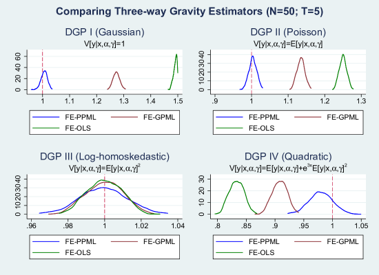
Figure 3: Kernel density plots of three-way gravity model estimates using different FE estimators, based on 500 replications. The model being estimated is $y_{ijt}=\exp[\alpha_{it}+\gamma_{jt}+\eta_{ij}+x_{ijt}\beta]\omega_{ijt}$, where the distribution of $\omega_{ijt}$ depends on the DGP and the true value of $\beta$ is 1 (indicated by the vertical dotted lines). The size of the $i$ and $j$ dimensions is given by $N=50$ and the $t$ dimension has size $T=5$. See text for further details.

To illuminate the unique IPP-robustness properties of FE-PPML in the three-way context, Fig. 3 shows a comparison of simulation results for FE-PPML versus log-OLS and Gamma PML. The displayed kernel densities are computed using 500 replications of a three-way panel structure with $N=50$ and $T=5$. The $i$ and $j$ dimensions of the panel both have size $N=50$ and the size of the time dimension is $T=5$. The fixed effects are generated according to the same procedures described in the text and we again model four different scenarios for the distribution of the error term (Gaussian, Poisson, Log-homoskedastic, and Quadratic).

As we would expect based on Proposition 2, FE-PPML is relatively unbiased across all four different assumptions considered for the distribution of the error term. The general inconsistency of the three-way OLS estimator—which is only unbiased for DGP III where the error term is log-homoskedastic—is also as expected. However, the reasons behind the bias in the OLS estimate are well-documented (see Santos Silva and Tenreyro, 2006) and do not have to do with the incidental parameters included in the model. The three-way FE-GPML estimator is also consistent under DGP III because it assumes the error term has a variance equal to the square of the conditional mean. Both OLS and GPML are also more efficient than PPML in this case. However, as the other three panels show, when this variance assumption is relaxed, three-way FE-GPML clearly suffers from an IPP, exhibiting an average bias equal to roughly half that of OLS in all three cases.

We have also performed some simulations with three-way FE-Gaussian PML, which imposes $g(\widehat{\lambda}_{ijt})=\widehat{\lambda}_{ijt}$. We do not show results for this other estimator because the HDFE-IRLS algorithm we used to produce the FE-PPML and FE-Gamma PML estimates frequently did not converge for the FE-Gaussian PML estimator. However, the results we did obtain were in line with our results for FE-GPML and with our discussion of Proposition 2 above: the FE-Gaussian PML estimates were consistent when the DGP for $\omega_{ijt}$ was itself Gaussian (as in DGP I), but were inconsistent otherwise.

A.6 Allowing for Conditional Dependence across Pairs

The bias expansion in Proposition 3 allows for errors to be clustered within each pair $(i,j)$, but assumes conditional independence of $y_{ij}$ and $y_{i^{\prime}j^{\prime}}$ for all $(i,j)\neq(i^{\prime},j^{\prime})$. This assumption is consistent with the standard practice in the literature of assuming that errors are clustered within pairs when computing standard errors (see Yotov, Piermartini, Monteiro, and Larch, 2016.) However, it is important to clarify that the results in Proposition 3 may change when other assumptions are used. For example, if we want to allow $y_{ij}$ and $y_{ji}$ (i.e., both directions of trade) to be correlated, then the bias results would not actually change, but we would need to modify the definition of $\Omega_{N}$ to allow for the additional clustering; namely, we would need

$$\Omega_{N} =\frac{1}{N\,(N-1)}\sum_{i=1}^{N-1}\sum_{j=i+1}^{N}{\rm Var}\left(\widetilde{x}_{ij}^{\prime}S_{ij}+\widetilde{x}_{ji}^{\prime}S_{ji}\,\big{|}\,x\right)$$

$$=\frac{1}{N\,(N-1)}\sum_{i=1}^{N-1}\sum_{j=i+1}^{N}\bigg{\{}\widetilde{x}_{ij}^{\prime}\,\left[{\rm Var}\left(S_{ij}\,\big{|}\,x_{ij}\right)\right]\,\widetilde{x}_{ij}+\widetilde{x}_{ji}^{\prime}\,\left[{\rm Var}\left(S_{ji}\,\big{|}\,x_{ji}\right)\right]\,\widetilde{x}_{ji}$$

$$\qquad\qquad\qquad\qquad\qquad+\widetilde{x}_{ij}^{\prime}\,\left[{\rm Cov}\left(S_{ij},S_{ji}\,\big{|}\,x_{ij}\right)\right]\,\widetilde{x}_{ji}+\widetilde{x}_{ji}^{\prime}\,\left[{\rm Cov}\left(S_{ji},S_{ij}\,\big{|}\,x_{ji}\right)\right]\,\widetilde{x}_{ij}\bigg{\}}.$$ (53)

Notice, however, this is just one possibility. Similar adjustments could be made to allow for clustering by exporter or importer, for example, or even for multi-way clustering à la Cameron, Gelbach, and Miller (2011). In these cases, the bias would also need to be modified; specifically, one would have to modify the portions of $D_{N}^{k}$ that $B_{N}^{k}$ that depend on the variance of $S_{ij}$ to allow for correlations across $i$ and/or $j$.

A.7 Showing Bias in the Cluster-robust Sandwich Estimator

For convenience, let $\mathbf{x}_{ij}:=(x_{ij},\,d_{ij})$ be the matrix of covariates associated with pair $ij$, inclusive of the $it$- and $jt$-specific dummy variables needed to estimate $\alpha_{i}$ and $\gamma_{j}$. Similarly, let $b:=(\beta^{\prime},\,\phi^{\prime})^{\prime}$ be the vector of coefficients to be estimated and let $\widehat{b}$ be the vector of coefficient estimates. Note that we can write a first-order approximation for $\widehat{S}_{ij}$ as

$$\widehat{S}_{ij} \approx S_{ij}-\bar{H}_{ij}\mathbf{x}_{ij}(\widehat{b}-b),$$

which is consistent with the approximation provided in (13). We can then replace $\widehat{b}-b$ with the standard first-order expansion $\widehat{b}-b\approx-\mathcal{\bar{L}}_{bb}^{-1}\mathcal{L}_{b}^{0}$, where $\mathcal{L}=\sum_{i,j}\ell_{ij}$ is the profile likelihood. This expansion in turn can be written out as

$$\widehat{b}-b \approx-\mathcal{\bar{L}}_{bb}^{-1}\left[\sum_{m,n}\mathbf{x}_{mn}^{\prime}S_{mn}\right].$$

Now we turn our attention to the outer product $\widehat{S}_{ij}\widehat{S}_{ij}^{\prime}$:

$$\widehat{S}_{ij}\widehat{S}_{ij}^{\prime} \approx S_{ij}S_{ij}^{\prime}+\bar{H}_{ij}\mathbf{x}_{ij}(\widehat{b}-b)^{2}\mathbf{x}_{ij}^{\prime}\bar{H}_{ij}-2\bar{H}_{ij}\left[\mathbf{x}_{ij}(\widehat{b}-b)\right]S_{ij}^{\prime}$$

$$=S_{ij}S_{ij}^{\prime}+\bar{H}_{ij}\mathbf{x}_{ij}(\widehat{b}-b)^{2}\mathbf{x}_{ij}^{\prime}\bar{H}_{ij}+2\bar{H}_{ij}\mathbf{x}_{ij}\mathcal{\bar{L}}_{bb}^{-1}\left[\sum_{m,n}\mathbf{x}_{mn}^{\prime}S_{mn}\right]S_{ij}^{\prime}$$

Because we assume we are in the special case where FE-PPML is correctly specified, we have that $\mathbb{E}[(\widehat{b}-b)^{2}]=-\kappa\mathcal{\bar{L}}_{bb}^{-1}$, where $\mathcal{\bar{L}}_{bb}:=\mathbb{E}[\mathcal{L}_{bb}]$. We also have that $\mathbb{E}[S_{ij}S_{ij}^{\prime}]=\kappa\bar{H}_{ij}$. Therefore, after applying expectations where appropriate, we have that

$$\mathbb{E}[\widehat{S}_{ij}\widehat{S}_{ij}^{\prime}] \approx S_{ij}S_{ij}^{\prime}+\kappa\bar{H}_{ij}\mathbf{x}_{ij}\mathcal{\bar{L}}_{bb}^{-1}\mathbf{x}_{ij}^{\prime}\bar{H}_{ij},$$

which can be seen as extending Kauermann and Carroll (2001)’s results to the case of a panel data pseudo-likelihood model with within-panel clustering. We are not done, however, as we have not yet isolated the influence of the incidental parameters. To complete the derivation of the bias, we must more carefully consider the full inverse Hessian term $\mathcal{\bar{L}}_{bb}^{-1}$. Using standard matrix algebra, this inverse can be written as:

$$\mathcal{\bar{L}}_{bb}^{-1}= \left(\!\!\begin{array}[]{cc}\left(\mathcal{\bar{L}}_{\beta\beta}-\mathcal{\bar{L}}_{\phi\beta}^{\prime}\bar{\mathcal{L}}_{\phi\phi}^{-1}\mathcal{\bar{L}}_{\phi\beta}\right)^{-1}&-\left(\bar{\mathcal{L}}_{\beta\beta}-\mathcal{\bar{L}}_{\phi\beta}^{\prime}\bar{\mathcal{L}}_{\phi\phi}^{-1}\bar{\mathcal{L}}_{\phi\beta}\right)^{-1}\mathcal{\bar{L}}_{\phi\beta}^{\prime}\bar{\mathcal{L}}_{\phi\phi}^{-1}\\ -\bar{\mathcal{L}}_{\phi\phi}^{-1}\mathcal{\bar{L}}_{\phi\beta}\left(\bar{\mathcal{L}}_{\beta\beta}-\bar{\mathcal{L}}_{\phi\beta}^{\prime}\mathcal{\bar{L}}_{\phi\phi}^{-1}\bar{\mathcal{L}}_{\phi\beta}\right)^{-1}&\mathcal{\bar{L}}_{\phi\phi}^{-1}\!+\mathcal{\bar{L}}_{\phi\phi}^{-1}\mathcal{\bar{L}}_{\phi\beta}\!\left(\bar{\mathcal{L}}_{\beta\beta}-\mathcal{\bar{L}}_{\phi\beta}^{\prime}\mathcal{\bar{L}}_{\phi\phi}^{-1}\mathcal{\bar{L}}_{\phi\beta}\right)^{-1}\!\mathcal{\bar{L}}_{\phi\beta}^{\prime}\bar{\mathcal{L}}_{\phi\phi}^{-1}\end{array}\!\!\right),$$

where we have used $\mathcal{\bar{L}}_{\phi\phi}$ in place of $\mathcal{\bar{H}}$ in order to add clarity. Making use of some already-established definitions, we have that the top-left term $(\mathcal{\bar{L}}_{\beta\beta}-\mathcal{\bar{L}}_{\phi\beta}^{*\prime}\bar{\mathcal{L}}_{\phi\phi}^{-1}\mathcal{\bar{L}}_{\phi\beta})^{-1}=-[N(N-1)]^{-1}W_{N}^{-1}$ and, similarly, that $\mathcal{\bar{L}}_{\phi\phi}^{-1}=-[N(N-1)]^{-1}W_{N}^{(\phi)-1}$. If we again consider $\mathbb{E}[\widehat{S}_{ij}\widehat{S}_{ij}^{\prime}]$, we can now write

$$\mathbb{E}[\widehat{S}_{ij}\widehat{S}_{ij}^{\prime}-S_{ij}S_{ij}^{\prime}] \approx-\frac{\kappa}{N(N-1)}\bar{H}_{ij}(x_{ij}\,d_{ij})\;\times$$

$$\left(\!\!\begin{array}[]{cc}W_{N}^{-1}&-W_{N}^{-1}\mathcal{\bar{L}}_{\phi\beta}^{\prime}\bar{\mathcal{L}}_{\phi\phi}^{-1}\\ -\bar{\mathcal{L}}_{\phi\phi}^{-1}\mathcal{\bar{L}}_{\phi\beta}W_{N}^{-1}&W_{N}^{(\phi)-1}\!\!+\mathcal{\bar{L}}_{\phi\phi}^{-1}\mathcal{\bar{L}}_{\phi\beta}^{*}W_{N}^{-1}\mathcal{\bar{L}}_{\phi\beta}^{\prime}\bar{\mathcal{L}}_{\phi\phi}^{*-1}\end{array}\!\!\right)\!(x_{ij}\,d_{ij})^{\prime}\bar{H}_{ij}$$

$$=-\frac{\kappa}{N(N-1)}\bar{H}_{ij}\left\{x_{ij}W_{N}^{-1}x_{ij}^{\prime}-x_{ij}W_{N}^{-1}\mathcal{\bar{L}}_{\phi\beta}^{\prime}\bar{\mathcal{L}}_{\phi\phi}^{-1}d_{ij}^{\prime}-d_{ij}\bar{\mathcal{L}}_{\phi\phi}^{-1}\mathcal{\bar{L}}_{\phi\beta}^{*}W_{N}^{-1}x_{ij}^{\prime}\right.$$

$$\left.+d_{ij}\mathcal{\bar{L}}_{\phi\phi}^{-1}\mathcal{\bar{L}}_{\phi\beta}W_{N}^{-1}\mathcal{\bar{L}}_{\phi\beta}^{\prime}\bar{\mathcal{L}}_{\phi\phi}^{-1}d_{ij}^{\prime}+d_{ij}W_{N}^{(\phi)-1}d_{ij}^{\prime}\right\}\bar{H}_{ij},$$

which simplifies to the expression shown in (13).

Results for the two-way model. Though we have focused on the downward bias of the sandwich estimator for the three-way gravity model, it is also known to be biased for the standard two-way gravity model without pair fixed effects (Egger and Staub, 2015; Jochmans, 2016; Pfaffermayr, 2019). As it turns out, the analytics for the two-way and three-way models are very similar here, and we can easily adapt our results to the simpler two-way setting. The main change we would need to make is to replace $H_{ij}$ everywhere it appears with $\Lambda_{ij}$, including in the definitions of $\widetilde{x}_{ij}$, $W_{N}$, and $W_{N}^{(\phi)}$. The rest of the derivations then follow in the same manner as for the three-way model. The resulting correction has been included in our ppml_fe_bias Stata package for users working with two-way gravity models. A version of this correction has been studied alongside other methods in a recent paper by Pfaffermayr (2021).

A.8 More Discussion of IPPs in FE-PPML Models

In this part of the Appendix, we wish to give a more expansive discussion of when IPPs may arise in case of an FE-PPML estimator. We have already reviewed the two-way and three-way gravity models in the main text; thus, here, we will focus first on the classic ‘‘one-way’’ FE panel setting where no IPP occurs. Doing so will allow us to draw a contrast with other, more complex models where IPPs could be a problem. As part of this discussion, we give some examples of panel models where FE-PPML is actually inconsistent, unlike the models covered in the main text.

The Classic (One-way) Setting

Consider a static panel data model with individuals $i=1,\ldots,N$, time periods $t=1,\ldots,T$, outcomes $y_{it}$, and strictly exogenous regressors $x_{it}$ satisfying

$$\mathbb{E}(y_{it}|x_{it},\alpha_{i}) =\lambda_{it}:=\exp(x_{it}^{\prime}\beta+\alpha_{i}).$$ (54)

The FE-PPML estimator maximizes $\sum_{i,t}\left(y_{it}\log\lambda_{it}+\lambda_{it}\right)$ over $\beta$ and $\alpha$. The corresponding FOC’s may be written as

$$\sum_{i=1}^{N}\sum_{t=1}^{T}\,x_{it}\,\left(y_{it}-\widehat{\lambda}_{it}\right) =0, \forall i:\;\;\sum_{t=1}^{T}\left(y_{it}-\widehat{\lambda}_{it}\right) =0,$$ (55)

where $\widehat{\lambda}_{it}:=\exp(x_{it}^{\prime}\widehat{\beta}+\widehat{\alpha}_{i})$. Solving for $\widehat{\alpha}_{i}$ and plugging the expression back into the FOC for $\widehat{\beta}$ we find

$$\sum_{i=1}^{N}\sum_{t=1}^{T}\,x_{it}\,\left[y_{it}-\frac{\exp(x_{it}^{\prime}\widehat{\beta})}{\sum_{\tau=1}^{T}\exp(x_{i\tau}^{\prime}\widehat{\beta})}\sum_{\tau=1}^{T}y_{i\tau}\right] =0,$$ (56)

which, as long as (54) holds, are valid (sample) moments to estimate $\beta$. Thus, under standard regularity conditions, we have that $\sqrt{N}(\widehat{\beta}-\beta^{0})\rightarrow_{d}{\cal N}(0,V)$ as $N\rightarrow\infty$, where $V$ is the asymptotic variance. The FE-PPML estimator therefore does not suffer from an IPP: even though $\widehat{\alpha}_{i}$ is an inconsistent estimate of $\alpha_{i}$, the FE-PPML score for $\beta$ has zero mean when evaluated at the true parameter $\beta^{0}$, and $\widehat{\beta}$ therefore converges in probability to $\beta^{0}$ without any asymptotic bias. This is a well known result that can also be obtained in the Poisson-MLE case by conditioning on $\sum_{t}y_{it}$; see Cameron and Trivedi (2015). For our purposes, it gives us a benchmark against which other, more complex models may be compared.

Examples where FE-PPML is Inconsistent

In the above ‘‘classic’’ setting, every observation is affected by exactly one fixed effect. In current applied work, it is common to specify models with what we will call ‘‘overlapping’’ fixed effects, where each observation may be affected by more than one fixed effects. Some standard examples include the gravity model from international trade (as is our focus in the main text) as well as other settings where researchers may wish to control for multiple sources of heterogeneity (e.g., firm and employee, teacher and student). Thus, it is important to clarify that the presence of overlapping fixed effects can easily lead to an IPP, even when the underlying estimator is Poisson or PPML. We give the following simple example:

Example 1.

Consider a model with three time periods $T=3$ and two fixed effects $\alpha_{i}$ and $\gamma_{i}$ for each individual:

$$t=1: \mathbb{E}(y_{i1}|x_{i1},\alpha_{i},\gamma_{i}) =\lambda_{i1}:=\exp(x_{i1}^{\prime}\beta+\alpha_{i}),$$

$$t=2: \mathbb{E}(y_{i2}|x_{i2},\alpha_{i},\gamma_{i}) =\lambda_{i2}:=\exp(x_{i2}^{\prime}\beta+\alpha_{i}+\gamma_{i}),$$

$$t=3: \mathbb{E}(y_{i3}|x_{i3},\alpha_{i},\gamma_{i}) =\lambda_{i3}:=\exp(x_{i3}^{\prime}\beta+\gamma_{i}).$$

The FE-PPML estimator maximizes $\sum_{i=1}^{N}\sum_{t=1}^{3}\left(y_{it}\log\lambda_{it}+\lambda_{it}\right)$ over $\beta$, $\alpha$ and $\gamma$. $T=3$ is fixed as $N\rightarrow\infty$.

Example 2.

In addition to $i=1,\ldots,N$ and $t=1,\ldots,T$ we re-introduce another panel dimension $j=1,\ldots,J$ and consider

$$\mathbb{E}(y_{ijt}|x_{ijt},\alpha_{it},\gamma_{ij}) =\lambda_{ijt}:=\exp(x_{ijt}^{\prime}\beta+\alpha_{it}+\gamma_{ij}),$$

where $\alpha_{it}$ is now indexed by both $i$ and $t$ and our second fixed effect is similarly indexed by $i$ and $j$. The FE-PPML estimator in this case maximizes $\sum_{i,j,t}\left(y_{ijt}\log\lambda_{ijt}+\lambda_{ijt}\right)$ over $\beta$, $\alpha$ and $\gamma$. We consider $N\rightarrow\infty$ with both $J$ and $T$ fixed, e.g. $J=T=2$.

In these examples, because the fixed effects are overlapping, we have that $\widehat{\alpha}$ enters into the FOC for $\widehat{\gamma}$, and vice versa. Therefore, when for a given value $\widehat{\beta}$ we want to solve the FOC for $\widehat{\alpha}$ and $\widehat{\gamma}$ we have to solve a system of equations, and the solutions become much more complicated functions of the outcome variable than in the one-way model. While having this type of co-dependence between the FOCs for the various fixed effects need not necessarily lead to an IPP, as we discuss next, it does create one in models where more than one fixed effect dimension grows at the same rate as the panel size, as is the case with $\alpha$ and $\gamma$ in both of these examples.

In gravity settings, by contrast, the crucial distinction is that the dimensions of each fixed effect grow only with the square root of the sample size as the number of countries increases. As mentioned in the text, this ensures that the IPPs associated with each fixed effect ‘‘decouple’’ from one another, in the sense described by Fernández-Val and Weidner (2016). However, in the inconsistency examples just given, the estimation noise in the estimated $\alpha$ parameters will always depend on the estimation noise in the estimated $\gamma$ parameters, and vice versa, even as $N\rightarrow\infty$. Thus, decoupling cannot occur. For illustration, we have used the model from Example 1 as our example of inconsistency in our earlier Figure 1. We have also performed simulations for the model in Example 2 and found similar results.

A Suggested Heuristic for IPPs when the Estimator is FE-PPML

As has been made clear from our discussion and results, the usual generic bias heuristic shown in (6) from Fernández-Val and Weidner (2018) is generally not appropriate for FE-PPML. Indeed, because FE-PPML can be asymptotically unbiased in special cases, it may not be productive to try to boil down how their biases are likely to behave to a single formula. Instead, we propose the following approach:

1. If there are no fixed effect dimensions that grow proportionately with the sample, we expect FE-PPML to be unbiased asymptotically.

2. Otherwise, the likely order of the bias can be derived as follows:

   1. Construct the equivalent multinomial model by profiling out the largest fixed effect dimension.

   2. Infer what the order of the asymptotic bias would be for the equivalent multinomial model by calculating $p/n$ (i.e., as in (6)).

For example, in the three-way gravity model, the number of observations is on the order of $N^{2}T$ and the number of parameters is on the order of $N^{2}$ pair fixed effects plus $2NT$ exporter-time and importer-time fixed effects. However, after profiling out the pair fixed effects, we only have the $2NT$ exporter-time and importer-time fixed effects. Thus, we take $p/n$ to be proportional to $1/N$ as $N\rightarrow\infty$, implying an asymptotic bias of order $1/N$.

For further illustration, consider Examples 1 and 2 above. In these cases, even after profiling out $\alpha$, one still finds that $p$ is proportional to $n$ as $n\rightarrow\infty$, implying inconsistency. As a contrast, consider the two-way gravity model. As we have just discussed, all of the fixed effects grow only with the square root of $n$ in that case, implying it is asymptotically unbiased.

‘‘Four-way’’ gravity models.

As a more complicated example, consider the following ‘‘four-way’’ gravity model:

$$y_{ijlt}=\exp{\left[\alpha_{ilt}+\alpha_{jlt}+\eta_{ijl}+\zeta_{ijt}+x_{ijlt}\beta\right]}\omega_{ijlt}.$$ (57)

This type of model may be used for trade data that is observed separately for different industries or commodities, which here are indexed by $l=1...L$. $\alpha_{ilt}$, $\alpha_{jlt}$, and $\eta_{ijl}$ respectively are industry-level analogs of $\alpha_{it}$, $\alpha_{jt}$, and $\eta_{ij}$ from the three-way model. Thus, they allow multilateral resistance effects and cross-sectional heterogeneity in trade costs to vary by industry. The fourth fixed effect, $\zeta_{ijt}$, captures general changes in trade across all industries for a given pair. $x_{ijlt}$ is assumed to be an industry-specific policy variable of interest (e.g., tariffs). We assume that the error term $\omega_{ijlt}$ exhibits correlation over time within the same exporter-importer-industry triplet but is independent across trade partners and across industries within the same exporter-importer pair.

The four-way model does not conform to the framework from our main analysis, but we can nonetheless use the above heuristic to infer the order of the bias and propose a correction. After profiling out the order-$N^{2}L$ exporter-importer-industry fixed effects, the model has on the order of $2NLT$ exporter-industry-time and importer-industry-time fixed effects and $N^{2}T$ exporter-importer-time fixed effects. The number of observations is on the order of $N^{2}LT$. Following our discussion from Section 2.2, the bias is thus expected to be of the form

$$\frac{1}{N}b^{(\alpha)}+\frac{1}{N}b^{(\gamma)}+\frac{1}{L}b^{(\zeta)}.$$ (58)

Where $b^{(\alpha)}$, $b^{(\gamma)}$, and $b^{(\zeta)}$ are unknown constants. Two observations stand out. First, for consistency, we require both $N$ and $L$ to be large. For data sets where the number of industries is relatively small, the $1/L$ bias term associated with the $\zeta_{ijt}$ fixed effect is likely to induce substantial bias. We will thus consider the implications for asymptotic bias as $N$ and $L$ grow large at the same rate. Second, the order of the standard error as $N$ and $L$ both $\rightarrow\infty$ while $T$ is fixed is $1/(N\sqrt{L})$. The ratio of the asymptotic bias to the standard error as $N$ and $L$ both $\rightarrow\infty$ is expected to be of the form

$$\frac{\sqrt{L}b^{(\alpha)}+\sqrt{L}b^{(\gamma)}+\frac{N}{\sqrt{L}}b^{(\zeta)}}{c},$$

where $c>0$ is a positive constant. This ratio diverges to infinity as $N,L\rightarrow\infty$, implying that the standard error shrinks to zero faster than the bias does. This is a more severe form of the asymptotic bias problem than the one we found for the three-way model, where the bias and standard error both decreased at the same rate asymptotically. It is therefore advised that a jackknife correction should be used to reduce the bias. This can be done by holding out industries to inflate the $1/L$ bias while simultaneuously holding out countries to inflate the $1/N$ bias. For example, a jackknife sample with half the number of countries and half the number of industries will have an asymptotic bias of order $2/N+2/L$.

A closely related model that we can also discuss is the case when the fourth fixed effect, $\zeta_{ijt}$, is not included in the model shown in (57). An example of when this might be desirable is when the policy variable of interest does not vary across industries (e.g., a trade agreement dummy). In this case, one can infer from the formula in (58) that we would expect an asymptotic bias of order $1/N$, like what we found in the case of the three-way model. Furthermore, if only the number of countries is allowed to become large, while both $L$ and $T$ are held fixed, the standard error is also of order $1/N$, and the behavior of the asymptotic bias is exactly like what we found for the three-way case. However, interestingly, if both $N$ and $L$ $\rightarrow\infty$, we are back in the case where the bias-to-standard error ratio heads to infinity. Thus, the severity of the problem will depend importantly on the number of industries in both of these models.

Finally, note that if $T$ is no longer fixed, so that $N$, $L$, and $T$ all $\rightarrow\infty$ jointly, we expect the special properties of PPML to cause the IPP bias to become more benign. We know from Fernández-Val and Weidner (2016)’s earlier results for the two-way model and from our own results for the three-way model that the decoupling of the IPPs as all dimensions of the panel become large at the same rate eliminates the asymptotic bias in these settings. Future work can investigate to what extent this holds true for four-way panel models.

References

- (1)
- Allen, Dobbin, and Morten (2018) Allen, T., C. d. C. Dobbin, and M. Morten (2018): “Border Walls,” Discussion paper, National Bureau of Economic Research.
- Alvarez and Arellano (2003) Alvarez, J., and M. Arellano (2003): “The Time Series and Cross-Section Asymptotics of Dynamic Panel Data Estimators,” Econometrica, 71(4), 1121–1159.
- Andersen (1970) Andersen, E. B. (1970): “Asymptotic properties of conditional maximum-likelihood estimators,” Journal of the Royal Statistical Society: Series B (Methodological), 32(2), 283–301.
- Anderson and van Wincoop (2003) Anderson, J. E., and E. van Wincoop (2003): “Gravity with Gravitas: A Solution to the Border Puzzle,” American Economic Review, 93(1), 170–192.
- Arellano and Bonhomme (2009) Arellano, M., and S. Bonhomme (2009): “Robust Priors in Nonlinear Panel Data Models,” Econometrica, 77(2), 489–536.
- Arellano and Hahn (2007) Arellano, M., and J. Hahn (2007): “Understanding Bias in Nonlinear Panel Models: Some Recent Developments,” Econometric Society Monographs, 43, 381.
- Bai (2009) Bai, J. (2009): “Panel Data Models With Interactive Fixed Effects,” Econometrica, 77(4), 1229–1279.
- Baier and Bergstrand (2007) Baier, S. L., and J. H. Bergstrand (2007): “Do Free Trade Agreements actually Increase Members’ International Trade?,” Journal of International Economics, 71(1), 72–95.