Multi-wavelength variability of the young solar analog $\iota$ Hor

Abstract

Context. Chromospheric activity cycles are common in late-type stars; however, only a handful of coronal activity cycles have been discovered. $\iota$ Hor is the most active and youngest star with known coronal cycles. It is also a young solar analog, and we are likely facing the earliest cycles in the evolution of solar-like stars, at an age ($\sim 600$ Myr) when life appeared on Earth.

Aims. Our aim is to confirm the $\sim$1.6 yr coronal cycle and characterize its stability over time. We use X-ray observations of $\iota$ Hor to study the corona of a star representing the solar past through variability, thermal structure, and coronal abundances.

Methods. We analyzed multi-wavelength observations of $\iota$ Hor using XMM-Newton, TESS, and HST data. We monitored $\iota$ Hor throughout almost seven years in X-rays and in two UV bands. The summed RGS and STIS spectra were used for a detailed thermal structure model, and the determination of coronal abundances. We studied rotation and flares in the TESS light curve.

Results. We find a stable coronal cycle along four complete periods, more than covered in the Sun. There is no evidence for a second longer X-ray cycle. Coronal abundances are consistent with photospheric values, discarding any effects related to the first ionization potential. From the TESS light curve we derived the first photometric measurement of the rotation period (8.2 d). No flares were detected in the TESS light curve of $\iota$ Hor. We estimate the probability of having detected zero flares with TESS to be $\sim 2$%.

Conclusions. We corroborate the presence of an activity cycle of $\sim$1.6 yr in $\iota$ Hor in X-rays, more regular than its Ca ii H&K counterpart. A decoupling of the activity between the northern and southern hemispheres of the star might explain the disagreement. The inclination of the system would result in an irregular behavior in the chromospheric indicators. The more extended coronal material would be less sensitive to this effect.

1 Introduction

Stellar activity is common among late-type stars, due to a combination of rotation and magnetism. Among the observational consequences are stellar spots, protuberances, coronal loops, flares, and activity cycles. The photospheric spots allow us to measure stellar rotation. Rotation slows down with time, thus the rotational period is a link with the stellar age (Skumanich, 1972). Stellar flares can reveal information of the dimensions on the active regions on the surface of the stars (Sanz-Forcada et al., 2007a; Reale, 2014, and references therein), but our knowledge of spot coverage and distribution over the stellar surface is still limited. The present-day Sun shows activity cycles with a dominating periodicity lasting $\sim$11 yr, although with some range in its duration (e.g., Hathaway, 2010) and well-known irregularities, such as the Maunder minimum, which also indicates a clear connection between the solar activity and the Earth’s climate, evident also in the infrared energy budget of the Earth’s thermosphere (Friis-Christensen & Lassen, 1991; Mlynczak et al., 2018, and references therein). It has been possible for some decades to search for the activity cycles in other late-type stars, allowing us to explore a range of values in the general variables behind the existence of these cycles. The Mount Wilson Ca ii H&K S-index survey was used by Baliunas et al. (1995, and references therein) to find that $\sim$60% of the main-sequence stars with spectral types from F to early M show chromospheric cycles with periods in the range $2.5-25$ yr. The very active (also youngest) stars tend to show irregular chromospheric variability rather than cycles. More mature stars with moderate levels of activity tend to show more stable cycles, while old inactive stars have no indication of cycles, which might be interpreted as a stage similar to the Maunder minimum (Testa et al., 2015).

Table 1: XMM-Newton observation log, OM flux density, exposure times of the EPIC and RGS instruments, and results of EPIC spectral fits

Date	XMM	OM Flux ($\times 10^{-12}$ erg s-1 cm-2 Å-1)		$t_{\rm exp}$ (ks)				$\log T_{1,2}$	$\log EM_{1,2}$	$L_{\rm X}$
	Rev.	UVM2	UVW2	pn	MOS 1	MOS 2	RGS	(K)	(cm-3)	($\times 10^{28}$ erg s-1)
2011-05-16	2094	1.899$\pm$0.040	…	5.0	7.32	7.2	15.6	6.57${}^{+0.03}_{-0.06}$, 6.88${}^{+0.03}_{-0.05}$	51.18${}^{+0.05}_{-0.12}$, 50.79${}^{+0.19}_{-0.13}$	5.65$\pm$0.07
2011-06-11	2107	…	…	5.9	14.2	14.3	29.4	6.58${}^{+0.02}_{-0.02}$, 6.92${}^{+0.02}_{-0.02}$	51.26${}^{+0.03}_{-0.03}$, 50.90${}^{+0.05}_{-0.05}$	7.08$\pm$0.06
2011-07-09	2121	1.960$\pm$0.040	…	6.9	9.18	9.2	19.2	6.58${}^{+0.02}_{-0.04}$, 6.89${}^{+0.01}_{-0.05}$	51.21${}^{+0.03}_{-0.10}$, 50.78${}^{+0.17}_{-0.07}$	5.93$\pm$0.06
2011-08-04	2134	1.914$\pm$0.038	…	6.1	8.47	8.41	17.6	6.59${}^{+0.03}_{-0.02}$, 6.95${}^{+0.03}_{-0.02}$	51.27${}^{+0.04}_{-0.04}$, 50.96${}^{+0.05}_{-0.10}$	7.47$\pm$0.07
2011-11-20	2188	1.928$\pm$0.048	…	5.5	7.55	7.67	16.0	6.59${}^{+0.03}_{-0.02}$, 6.96${}^{+0.03}_{-0.02}$	51.19${}^{+0.05}_{-0.05}$, 51.02${}^{+0.05}_{-0.08}$	7.24$\pm$0.07
2011-12-18	2202	1.877$\pm$0.045	…	4.86	6.95	7.03	14.6	6.57${}^{+0.02}_{-0.03}$, 6.94${}^{+0.03}_{-0.02}$	51.17${}^{+0.04}_{-0.04}$, 50.78${}^{+0.07}_{-0.09}$	5.52$\pm$0.07
2012-01-15	2216	1.822$\pm$0.042	…	4.56	6.64	6.68	13.9	6.59${}^{+0.04}_{-0.07}$, 6.88${}^{+0.04}_{-0.05}$	51.05${}^{+0.07}_{-0.16}$, 50.75${}^{+0.20}_{-0.18}$	4.65$\pm$0.06
2012-02-10	2229	1.835$\pm$0.034	…	7.42	9.72	9.91	20.4	6.53${}^{+0.05}_{-0.07}$, 6.83${}^{+0.07}_{-0.05}$	50.99${}^{+0.09}_{-0.13}$, 50.69${}^{+0.17}_{-0.26}$	3.86$\pm$0.05
2012-05-19	2279	1.844$\pm$0.043	…	6.19	8.48	8.51	17.6	6.48${}^{+0.06}_{-0.05}$, 6.85${}^{+0.05}_{-0.02}$	50.98${}^{+0.09}_{-0.07}$, 50.81${}^{+0.07}_{-0.17}$	4.34$\pm$0.06
2012-06-29	2299	1.790$\pm$0.029	…	9.73	12.3	12.3	25.6	6.55${}^{+0.02}_{-0.12}$, 6.90${}^{+0.02}_{-0.07}$	51.11${}^{+0.03}_{-0.07}$, 50.77${}^{+0.23}_{-0.06}$	5.01$\pm$0.05
2012-08-09	2320	1.853$\pm$0.036	…	6.7	8.73	9.0	18.6	6.48${}^{+0.07}_{-0.05}$, 6.83${}^{+0.04}_{-0.02}$	50.95${}^{+0.11}_{-0.07}$, 50.93${}^{+0.06}_{-0.15}$	4.83$\pm$0.06
2012-11-18	2371	1.853$\pm$0.031	…	3.99	6.13	5.79	17.0	6.56${}^{+0.03}_{-0.10}$, 6.88${}^{+0.04}_{-0.06}$	51.13${}^{+0.06}_{-0.17}$, 50.78${}^{+0.22}_{-0.14}$	5.24$\pm$0.07
2012-12-20	2387	1.851$\pm$0.044	…	4.49	5.53	6.46	13.6	6.57${}^{+0.03}_{-0.08}$, 6.88${}^{+0.03}_{-0.05}$	51.08${}^{+0.07}_{-0.16}$, 50.83${}^{+0.17}_{-0.14}$	5.17$\pm$0.07
2013-02-03	2409	1.848$\pm$0.036	…	6.44	7.51	8.75	18.1	6.53${}^{+0.05}_{-0.09}$, 6.87${}^{+0.04}_{-0.04}$	51.01${}^{+0.09}_{-0.14}$, 50.85${}^{+0.13}_{-0.15}$	4.69$\pm$0.06
2013-05-20	2462	…	1.673$\pm$0.009	4.5	6.25	6.5	13.6	6.57${}^{+0.03}_{-0.03}$, 6.91${}^{+0.02}_{-0.02}$	51.16${}^{+0.05}_{-0.06}$, 51.00${}^{+0.07}_{-0.06}$	6.79$\pm$0.08
2013-08-09	2503	…	1.657$\pm$0.006	9.86	11.8	12.3	24.8	6.58${}^{+0.03}_{-0.04}$, 6.87${}^{+0.04}_{-0.04}$	51.20${}^{+0.06}_{-0.09}$, 50.87${}^{+0.14}_{-0.16}$	6.33$\pm$0.06
2014-02-05	2593	…	1.669$\pm$0.008	6.3	8.24	8.4	17.6	6.57${}^{+0.02}_{-0.04}$, 6.90${}^{+0.02}_{-0.05}$	51.15${}^{+0.03}_{-0.08}$, 50.70${}^{+0.16}_{-0.06}$	5.07$\pm$0.06
2014-05-18	2644	…	1.677$\pm$0.006	9.22	11.1	11.7	24.2	6.58${}^{+0.01}_{-0.02}$, 6.90${}^{+0.02}_{-0.05}$	51.13${}^{+0.02}_{-0.05}$, 50.50${}^{+0.16}_{-0.08}$	4.31$\pm$0.05
2014-08-11	2687	…	1.673$\pm$0.007	9.31	11.1	11.8	24.4	6.60${}^{+0.01}_{-0.01}$, 6.91${}^{+0.03}_{-0.03}$	51.29${}^{+0.02}_{-0.03}$, 50.71${}^{+0.10}_{-0.09}$	6.56$\pm$0.06
2014-11-20	2738	…	1.658$\pm$0.009	5.6	7.49	7.73	16.2	6.57${}^{+0.02}_{-0.02}$, 6.92${}^{+0.02}_{-0.02}$	51.26${}^{+0.03}_{-0.04}$, 51.00${}^{+0.05}_{-0.05}$	7.69$\pm$0.08
2015-02-06	2777	…	1.683$\pm$0.002	4.48	6.08	6.44	13.6	6.56${}^{+0.04}_{-0.08}$, 6.87${}^{+0.03}_{-0.04}$	51.18${}^{+0.08}_{-0.15}$, 51.04${}^{+0.14}_{-0.12}$	7.21$\pm$0.08
2015-05-21	2829	1.819$\pm$0.001	1.669$\pm$0.002	4.51	6.08	6.38	13.6	6.59${}^{+0.04}_{-0.05}$, 6.87${}^{+0.07}_{-0.05}$	51.13${}^{+0.07}_{-0.12}$, 50.67${}^{+0.22}_{-0.27}$	4.86$\pm$0.07
2015-08-11	2870	1.857$\pm$0.001	1.654$\pm$0.002	4.48	6.25	6.49	13.6	6.60${}^{+0.02}_{-0.04}$, 6.90${}^{+0.14}_{-0.18}$	51.09${}^{+0.03}_{-0.16}$, 49.97${}^{+0.68}_{-0.74}$	3.30$\pm$0.06
2015-11-21	2921	1.872$\pm$0.001	1.714$\pm$0.002	6.95	9.0	9.3	19.2	6.57${}^{+0.03}_{-0.05}$, 6.85${}^{+0.05}_{-0.04}$	51.13${}^{+0.07}_{-0.10}$, 50.76${}^{+0.16}_{-0.21}$	5.17$\pm$0.06
2016-02-06	2960	1.855$\pm$0.001	…	4.89	6.86	6.98	14.7	6.59${}^{+0.04}_{-0.05}$, 6.84${}^{+0.06}_{-0.04}$	51.17${}^{+0.08}_{-0.12}$, 50.78${}^{+0.18}_{-0.29}$	5.53$\pm$0.07
2016-06-25	3030	…	1.669$\pm$0.001	8.84	11.2	11.4	23.6	6.57${}^{+0.02}_{-0.02}$, 6.93${}^{+0.02}_{-0.01}$	51.25${}^{+0.03}_{-0.03}$, 50.97${}^{+0.04}_{-0.05}$	7.38$\pm$0.06
2016-07-07	3036	…	1.704$\pm$0.001	5.37	7.4	7.62	15.8	6.59${}^{+0.03}_{-0.03}$, 6.91${}^{+0.02}_{-0.03}$	51.19${}^{+0.04}_{-0.06}$, 50.87${}^{+0.10}_{-0.08}$	6.27$\pm$0.07
2017-02-04	3142	…	1.695$\pm$0.001	8.33	11.0	11.0	21.5	6.45${}^{+0.03}_{-0.04}$, 6.83${}^{+0.01}_{-0.01}$	51.07${}^{+0.05}_{-0.06}$, 51.09${}^{+0.04}_{-0.05}$	6.75$\pm$0.06
2017-05-20	3195	1.726$\pm$0.001	1.659$\pm$0.001	5.93	9.76	9.88	21.5	6.59${}^{+0.02}_{-0.04}$, 6.87${}^{+0.03}_{-0.05}$	51.19${}^{+0.04}_{-0.09}$, 50.68${}^{+0.20}_{-0.16}$	5.37$\pm$0.06
2017-08-10	3236	1.729$\pm$0.001	…	4.4	6.48	6.54	13.6	6.54${}^{+0.04}_{-0.06}$, 6.84${}^{+0.07}_{-0.05}$	51.12${}^{+0.09}_{-0.11}$, 50.73${}^{+0.17}_{-0.30}$	4.86$\pm$0.07
2017-11-20	3287	1.799$\pm$0.001	1.647$\pm$0.002	5.24	7.37	7.49	15.6	6.59${}^{+0.03}_{-0.02}$, 6.92${}^{+0.03}_{-0.02}$	51.24${}^{+0.04}_{-0.04}$, 50.87${}^{+0.06}_{-0.09}$	6.69$\pm$0.07
2018-02-03	3325	1.755$\pm$0.001	1.646$\pm$0.001	13.2	13.1	13.3	27.4	6.59${}^{+0.03}_{-0.01}$, 6.95${}^{+0.03}_{-0.01}$	51.38${}^{+0.04}_{-0.02}$, 51.11${}^{+0.03}_{-0.09}$	10.10$\pm$0.07

With the arrival of the large X-ray observatories, XMM-Newton and Chandra, an interest in coronal cycles has been triggered. The first discoveries of coronal cycles were made in several stars with previously known chromospheric activity cycles: HD 81809 (Favata et al., 2004, 2008; Orlando et al., 2017), 61 Cyg A (Hempelmann et al., 2006; Robrade et al., 2012; Boro Saikia et al., 2016), and $\alpha$ Cen B (Robrade et al., 2005, 2012; Ayres, 2009; DeWarf et al., 2010), all of them in binary systems. The two components of $\alpha$ Cen and 61 Cyg are resolved spatially in X-rays, and tentative cycles have been proposed, but not yet confirmed, for the companions 61 Cyg B and $\alpha$ Cen A (Robrade et al., 2012; Ayres, 2014) and for Proxima Cen (Wargelin et al., 2017). All of them have in common their relatively old ages ($>2$ Gyr, Barnes, 2007) and their long rotation periods. Younger stars have shorter rotation periods and higher levels of activity. The search for coronal cycles has shown seasonal changes in EK Dra and AB Dor (Güdel, 2004; Sanz-Forcada et al., 2007b), but no evidence of cycles after 35 years of X-ray monitoring of the very active star AB Dor (Lalitha & Schmitt, 2013). The shortest coronal cycle found to date is that of $\iota$ Hor (1.6 yr, Sanz-Forcada et al. 2013, hereafter SSM13, ), being also the youngest and most active star for which a coronal cycle has been identified. A very similar level of activity is present in $\epsilon$ Eri, for which a $\sim$2.9 yr coronal cycle has recently been found (Coffaro et al., submitted). Wargelin et al. (2017) found a cycle in the dwarf M5.5 star Proxima Cen, with X-ray data that are partly consistent with the photospheric counterpart, and an X-ray amplitude $L_{\rm Xmax}/L_{\rm Xmin}\sim 1.5-2$. These authors also find a positive correlation between the X-ray activity cycle amplitude and Rossby number (assuming that Proxima Cen and $\alpha$ Cen A X-ray cycles are real).

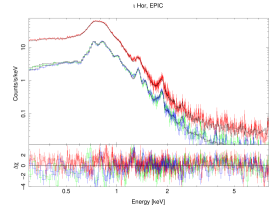
Figure 1: Spectral fit (black) for the summed XMM-Newton/EPIC-pn observation of $\iota$ Hor for a total of 168, 228, and 234 ks in pn (red), MOS1 (green), and MOS2 (blue), respectively. The spectra include $1\sigma$ error bars.

$ι$ Hor (HR 810, HD 17051) is an F8V/G0V star (Vauclair et al., 2008) at a distance of 17.24$\pm 0.16$ pc (van Leeuwen, 2007). A giant ($M\sin i=2.48$ M_J) planet was found orbiting $\iota$ Hor at 0.96 a.u. (Kürster et al., 2000; Zechmeister et al., 2013). In SSM13 we studied in detail this moderately active star ($\log L_{\rm X}/L_{\rm bol}=-4.9$, $\log R^{\prime}_{\rm HK}=-4.6$), and established for the first time the presence of a coronal (X-ray) cycle of the same duration as the chromospheric 1.6 yr cycle reported by Metcalfe et al. (2010). With an age of $\sim$600 Myr (SSM13, , and references therein), it can be considered a young solar analog. $\iota$ Hor allows us to study the radiation environment at the approximate age at which life appeared on Earth (Cnossen et al., 2007, and references therein). It is the earliest solar-like activity cycle discovered to date. A detailed study of the corona of $\iota$ Hor is of great importance not only for the knowledge of the evolution of activity cycles with stellar age, but also for our understanding of other coronal parameters of the young Sun, such as coronal thermal structure or abundances. Given the few cases of late-type stars with accurate measurements of their coronal and photospheric abundances, we can put it in the context of the fractionation effects that take place in the solar corona itself. In this work we continue the analysis of the coronal cycle of $\iota$ Hor where we explore the existence of a second, longer cycle, suggested by earlier data in SSM13 and Sanz-Forcada & Stelzer (2016). This study complements the long-term study of the magnetic field of $\iota$ Hor whose initial results are presented in Alvarado-Gómez et al. (2018b). In that study we proposed that the time-evolution of chromospheric activity can be described by a superposition of two periodic signals with similar amplitude, at $P_{1}\simeq 1.97$ and $P_{2}\simeq 1.41$ yr. We also estimate a rotation period of $P_{\rm rot}=7.70^{+0.18}_{-0.67}$ d, close to the proposed values in the range 7.9–8.5 d from photometry and Ca ii variations (Vauclair et al., 2008; Metcalfe et al., 2010). A second longer chromospheric cycle with irregular amplitude is suggested by the Ca ii H&K data of Flores et al. (2017), with a $P_{\rm cyc}\sim 4.57$ yr, but the shorter 1.6 yr cycle was not identified in the same data set.

Table 2: Coronal and photospheric abundances of $\iota$ Hor (solar units)

	FIP	Solar photosphere		$\iota$ Hor [X/H]
X	(eV)	Ref.a	(AG89)	RGS	EPIC	Photosphere
Al	5.98	6.45	6.47	0.29$\pm$0.19	…	0.17$\pm$0.04
Ni	7.63	6.22	(6.25)	0.15$\pm$0.22	…	0.14$\pm$0.05
Mg	7.64	7.60	(7.58)	-0.09$\pm$0.28	0.13$\pm$0.03	0.17$\pm$0.05
Si	8.15	7.51	(7.56)	0.41$\pm$0.18	-0.02$\pm$0.04	0.16$\pm$0.05
Fe	7.87	7.50	(7.67)	0.14	0.14$\pm$0.02	0.19$\pm$0.06
S	10.36	7.12	(7.21)	-0.09$\pm$0.35	…	…
C	11.26	8.43	(8.56)	-0.04$\pm$0.13	…	0.21$\pm$0.08
O	13.61	8.69	(8.93)	0.26$\pm$0.10	-0.01$\pm$0.03	0.16$\pm$0.08
N	14.53	7.83	(8.05)	0.24$\pm$0.13	…	…
Ar	15.76	6.40	(6.56)	0.78$\pm$0.39	…	…
Ne	21.56	7.93	(8.09)	0.13$\pm$0.15	0.00$\pm$0.06	…

In Sect. 2 we describe the observations and the analysis carried out, and we explain the results in Sect. 3. We discuss the results in the general framework of stellar coronae, and stellar activity in Sect. 4, and present the conclusions in Sect. 5.

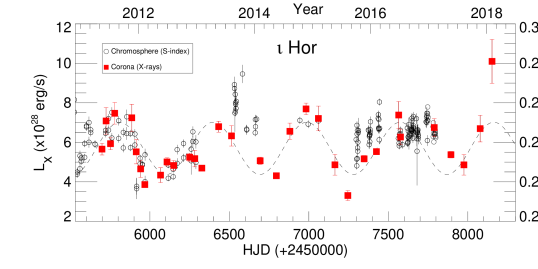
Figure 2: Time series of X-ray luminosity and chromospheric S-index for $\iota$ Hor. The dashed line indicates the cycle calculated using just coronal X-ray data (period of 588.5 d). The error bars of coronal X-ray luminosity are based on the standard deviation within each snapshot. Chromospheric data from SSM13 and Alvarado-Gómez et al. (2018b).

2 Observations

This work benefited from the information provided by different instruments covering X-rays, UV, and optical wavelength ranges, including photometric and spectroscopic information, as described below.

2.1 XMM-Newton

We monitored the X-ray emission of $\iota$ Hor between May 2012 and February 2018 using XMM-Newton (proposal IDs 067361, 069355, 072247, 074402, 076383, 080338, P.I. J. Sanz-Forcada; and Director Discretionary Time proposals 070198, 079018), for a total of 32 snapshots of 7–15 ks of total duration (Table 1 lists the effective exposures from each instrument). XMM-Newton allows the simultaneous use of all instruments on board.

2.1.1 EPIC and RGS

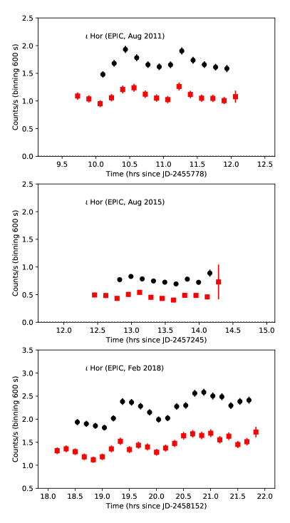
Figure 11: Time series for the XMM-Newton EPIC (black, pn + MOS1 + MOS2) and MOS (red, MOS1+MOS2) observations of $\iota$ Hor during the lowest activity level and highest flaring activity, with 1$\sigma$ error bars. MOS data are scaled up ($\times 2$) for a better display with EPIC data. MOS observations start earlier than EPIC-pn exposures. The count rate scale of the February 2018 observation is larger than the others.

Data from the X-ray detectors were reduced following standard procedures present in the Science Analysis Software (SAS) package v16.1.0, removing the time intervals with high background. The European Imaging Photon Camera (EPIC) PN and MOS (sensitivity range 0.1–15 keV and 0.2–10 keV, respectively, $E/\Delta E\sim 20-50$, Turner et al., 2001; Strüder et al., 2001) were used to monitor the long- and short-term X-ray variability of the star. EPIC light curves (Fig. 11) and spectra were extracted for each observation. All EPIC and Reflection Grating Spectrometer (RGS) spectra were fit using the ISIS package (Houck & Denicola, 2000) and the Astrophysics Plasma Emission Database (APED, Foster et al., 2012) v3.0.9. We summed all EPIC spectra, separately for PN, MOS1, and MOS2, and we simultaneously fit them to accurately calculate the coronal abundance of Fe, O, Ne, Mg, and Si (Fig. 1). The summed EPIC spectra were fit using a global 3-T model: $\log T_{1,2,3}$(K)=$6.15\pm 0.02$, $6.64\pm 0.01$, $6.92\pm 0.01$; $\log$ EM_1,2,3 (cm^-3)=$50.95\pm 0.06$, $51.12\pm 0.02$, $50.81\pm 0.02$, resulting in the abundances given in Table $a$. A low value of interstellar medium (ISM) absorption H column density of 3$\times 10^{18}$ cm^-3 was adopted, consistent with the fit to the overall spectrum, and the distance to the source (17.2 pc). Global 2-T fits were used for the spectra of each observation, fixing abundances to those of the summed spectrum. Results of these fits are displayed in Table 1. The X-ray luminosity ($L_{\rm X}=7.93\pm 0.01\times 10^{28}$ in the summed spectra) was calculated in the usual ROSAT band 0.12–2.48 keV from the best-fit model (Fig. 2).

The RGS ($\lambda\lambda\sim 6-38$ Å, $\lambda$/$\Delta\lambda\sim$100–500, den Herder et al., 2001) spectra were summed to get an overall, time-averaged, high spectral resolution view of the corona of $\iota$ Hor (Fig. 3). In the case of RGS a more complex procedure was employed to benefit from the rich information provided by the measurements of mostly resolved spectral lines. This information was used to construct an emission measure distribution (EMD) multi-T model ($\Delta T=0.1$ dex) following Sanz-Forcada et al. (2003). Spectral line fluxes with blend contributions, and comparison with the line fluxes predicted by the model are listed in Table 6. In this method line fluxes are measured considering the local continuum predicted by an initial 2-T model (see Fig. 3 with local continuum at the end of the process), convolving the response of the instrument with the lines. The measured lines are compared with the fluxes predicted by an initial EMD model. The observed ratios allow the model to be changed in order to search for the best ratios. The whole process is iterated to place a better continuum until the results converge (Table 3, Fig. 4). The [Fe/H] abundance is fixed to the value determined with EPIC, where the continuum is more sensitive to this parameter than the RGS continuum. This method also allows the abundances of some elements in the corona to be measured, as shown in Table $a$ and Fig. 5.

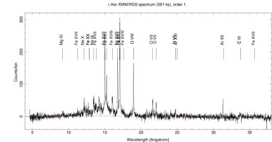
Figure 3: XMM-Newton/RGS (RGS1 + RGS2) summed spectrum of all observations, for a total of 591 ks. A dashed red line indicates the continuum below the emission lines.

2.1.2 The Optical Monitor

The XMM-Newton Optical Monitor (OM) was used to observe $\iota$ Hor either in “Image” or “Time Series” modes in the UV, with the UVW2 ($\lambda=2120\AA$, $\Delta\lambda=500\AA$) and UVM2 ($\lambda=2310\AA$, $\Delta\lambda=480\AA$) filters in the different campaigns. We used the OM data as processed in the official XMM-Newton pipeline products. The UV flux densities in these bands during the different exposures are listed in Table 1. By averaging all OM observations for a given filter we found a mean observed flux density of $F_{\rm UVM2}=(1.84\pm 0.06)\ 10^{-12}\,\rm erg\,s^{-1}cm^{-2}\AA^{-1}$ for the UVM2 band and $F_{\rm UVW2}=(1.67\pm 0.01)\ 10^{-12}\,\rm erg\,s^{-1}cm^{-2}\AA^{-1}$ for the UVW2 band. In Sect. 4.4 we use these values together with the flux densities predicted from photospheric model atmospheres to calculate the chromospheric contribution to the UV flux of $\iota$ Hor.

2.2 HST

We acquired Hubble Space Telescope (HST) observations on 2018 Sep 3 through HST Proposal ID 15299 (P.I. J. D. Alvarado-Gómez), using the Space Telescope Imaging Spectrograph (STIS) with the E140M grating (sensitivity range $1150-1740\leavevmode\nobreak\ \AA$, $\lambda/\Delta\lambda=11500-17400$). Two observations of 3141 s of exposure time each were summed using IRAF STIS package software, to get a better quality spectrum. We then measured the line flux of lines formed in the $\log T$(K)$=4.1-5.6$ range to extend our EMD analysis towards the transition region and upper chromosphere of $\iota$ Hor. Two lines, C ii 1334.535 Å and Si iv 1402.7704 Å, were affected by the ISM absorption in less than $\sim 20\%$. In these two cases the line flux was measured by fitting a Gaussian to the emission line. All line wavelengths and measured fluxes are listed in Table 7.

2.3 TESS

We explored the data from NASA’s Transiting Exoplanet Survey Satellite (TESS) mission (Ricker et al., 2015) to calculate the rotational period of $\iota$ Hor and to assess its photometric activity. The short-cadence (2 minutes) data of $\iota$ Hor were collected by TESS in sector 2 and sector 3, starting on 2018 Aug 23 and 2018 Sep 20, respectively, and were made publicly available with the first data release in December 2018 and January 2019. The target pixel file, which consists of 19737 and 19692 cadences for sectors 2 and 3, respectively, was downloaded from the Barbara A. Mikulski Archive for Space Telescopes (MAST) Portal. The light curves were obtained using the KeplerGO/lightkurve code (version: 1.0b13, August 2018; Lightkurve Collaboration et al., 2018). To create the apertures that were used to extract the light curves from the target pixel files, all cadences from one sector were summed into a single image. Then all the pixels of this combined image that have a value within a certain percentage of the maximum flux value were used in the extraction aperture. Ten different apertures with 0.1, 0.2, 0.3, 0.4, 0.5, 1, 2, 3, 4, and 5% of the maximum flux value were tested. The light curve with the lowest standard deviation was chosen as the final one. The aperture that was used to extract the final light curve consisted of all pixels with flux values higher than 0.2% and 0.4% of the maximum value for sectors 2 and 3 light curves, respectively.

TESS assigns a quality flag to all measurements. We removed all the flagged data points except “Impulsive outlier” and “Cosmic ray in collateral data” (bits 10 and 11) while extracting the light curve. The final light curve, which is shown in Fig. 6, consists of 31770 data points. It shows a quasi-periodic variation with an amplitude below the percent level. Such variability is typical for rotating star spots.

3 Results

The variety of observations analysed give a rich number of results. We present first the results from the X-rays photometric analysis, then the combination of X-rays and UV spectroscopy, UV photometry, and optical light curves.

3.1 X-ray variability

Short-term X-ray variability $(f_{\rm max}-f_{\rm min})/f_{\rm min}\la 40\%$ is observed during almost all epochs, but no large flares were identified. Small flares lasting up to $\sim$1 hr could be present in August 2011 and February 2018 (Fig. 11). The X-ray luminosity $L_{\rm X}$ displays a remarkably stable variability pattern. The X-ray amplitude ($L_{\rm Xmax}$/$L_{\rm Xmin}$) is 2.3 in the standard $0.12-2.48$ keV band, except for the last maximum of the series (February 2018), with a value three times larger than the minimum reached in August 2018 (Fig. 2). This maximum could be affected by a larger scale flaring activity; we note the increasing flux level and the two flares in the light curve of this interval (Fig. 11).

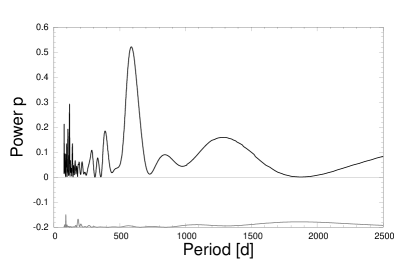
Figure 7: Generalized Lomb–Scargle power spectrum (top panel) and window function (bottom panel) of the long-term X-ray light curve of $\iota$ Hor. The significant peak is at $587$ d.

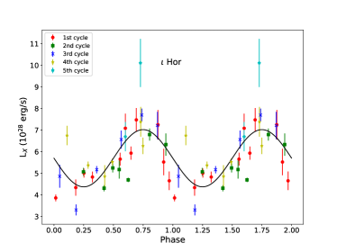
Figure 8: Phase-folded long-term X-ray light curve of $\iota$ Hor  based on the period of $588.5$ d, obtained from the GLS periodogram analysis described in Sect. 3.1. Superposed is the corresponding sine curve.

We used the X-ray luminosity values from all observations to calculate a periodogram using the generalized Lomb-Scargle (GLS) software, implemented by Zechmeister & Kürster (2009). The Lomb-Scargle (LS) periodogram is shown in Fig. 7. The only significant peak is at $587$ d. The X-ray light curve phase-folded with this period is shown in Fig. 8, overlaid with the sinusoid corresponding to this highest peak in the periodogram. The mean X-ray luminosity and the half-amplitude of the X-ray cycle obtained from the sinusoid are $\langle L_{\rm x}\rangle=5.8\times 10^{28}\,{\rm ergs^{-1}}$ and $\Delta L_{\rm x}=1.4\times 10^{28}\,{\rm ergs^{-1}}$, respectively, i.e., $\Delta L_{\rm x}/\langle L_{\rm x}\rangle=24$ %. The error associated with the period was found through Monte Carlo simulations: each value of the X-ray luminosity in the light curve was considered as the mean of a normal distribution, and from this a set of 1000 normally distributed random numbers was generated for each data point. We thus obtained 1000 simulated X-ray light curves on which we performed the LS analysis. The distribution of the resulting periods is a Gaussian. We adopt the peak of this distribution and its standard deviation, $588.5\pm 5.5$ d, as the period of the X-ray cycle and its uncertainty. The TESS and HST observations took place near the expected minimum of the activity cycle.

Table 3: Emission measure distribution of $\iota$ Hor.

log $T$ (K)	EM (cm-3)	log $T$ (K)	EM (cm-3)
4.0	51.15:	5.8	48.35${}^{+0.20}_{-0.30}$
4.1	51.05:	5.9	48.45${}^{+0.30}_{-0.30}$
4.2	50.85:	6.0	48.75${}^{+0.30}_{-0.20}$
4.3	50.65${}^{+0.30}_{-0.10}$	6.1	48.95${}^{+0.20}_{-0.30}$
4.4	50.45${}^{+0.10}_{-0.30}$	6.2	49.50${}^{+0.30}_{-0.20}$
4.5	50.25${}^{+0.10}_{-0.30}$	6.3	49.85${}^{+0.20}_{-0.10}$
4.6	49.95${}^{+0.10}_{-0.30}$	6.4	49.55${}^{+0.30}_{-0.20}$
4.7	49.85${}^{+0.20}_{-0.20}$	6.5	49.65${}^{+0.30}_{-0.20}$
4.8	49.75${}^{+0.40}_{-0.10}$	6.6	49.75${}^{+0.40}_{-0.20}$
4.9	49.70${}^{+0.30}_{-0.10}$	6.7	50.40${}^{+0.20}_{-0.10}$
5.0	49.75${}^{+0.10}_{-0.20}$	6.8	50.70${}^{+0.10}_{-0.10}$
5.1	49.75${}^{+0.10}_{-0.20}$	6.9	49.95${}^{+0.40}_{-0.10}$
5.2	49.45${}^{+0.10}_{-0.30}$	7.0	50.05${}^{+0.10}_{-0.10}$
5.3	49.25${}^{+0.10}_{-0.30}$	7.1	49.35${}^{+0.20}_{-0.20}$
5.4	48.90${}^{+0.10}_{-0.30}$	7.2	48.70${}^{+0.20}_{-0.30}$
5.5	48.45${}^{+0.20}_{-0.20}$	7.3	47.75:
5.6	48.25${}^{+0.20}_{-0.30}$	7.4	47.55:
5.7	48.25${}^{+0.20}_{-0.20}$	7.5	47.35:

.

3.2 Emission measure distribution and abundances

The EMD (Fig. 4, Table 3), determined as explained above from the summed RGS and STIS spectra of all observations, shows a moderately active star with a main peak at $\log T$ (K)=6.8 and a lower peak at $\log T$ (K)=6.3 resembling that of low-activity stars like the Sun or $\alpha$ Cen B (Orlando et al., 2000; Sanz-Forcada et al., 2011). Some material at temperatures above 10 MK is also found, but less abundant than in very active stars such as AB Dor. The corona of $\iota$ Hor has similar characteristics to that of $\epsilon$ Eri (Sanz-Forcada et al., 2004) or $\kappa$ Cet (Cnossen et al., 2007). Loop models show that the highest EM is found at the maximum temperature of the loop (e.g., Griffiths & Jordan, 1998; Cargill & Klimchuk, 2006). Therefore, the EMD of $\iota$ Hor can be interpreted as the result of a combination of loops with their maximum temperatures at the two mentioned peaks. The lower temperature is not identified in the EPIC spectra because the global fitting methods yield the dominant temperatures, and material at $\log T$ (K)=6.6 (found in EPIC fits) has an EM similar to the average of the peak at $\log T$ (K)=6.2–6.4. Thanks to the UV lines observed with STIS, our coronal model (the EMD) is extended to the transition region and upper chromosphere. This allows us to estimate the flux in different extreme ultraviolet (EUV) bands useful for evaluating the impact on exoplanet atmospheres, following the method explained in Sanz-Forcada et al. (2011): $L_{100-920\AA}=1.7\times 10^{29}$ erg s^-1, $L_{100-504\AA}=5.5\times 10^{28}$ erg s^-1.

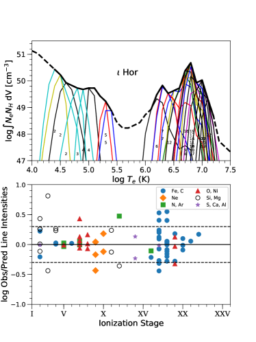
Figure 4: Upper panel: Emission measure distribution of $\iota$ Hor calculated using the summed RGS spectrum. The thin lines represent the relative contribution function for each ion (the emissivity function multiplied by the EMD at each point). The small numbers indicate the ionization stages of the species. Lower panel: Shown are the observed-to-predicted line flux ratios for the ion stages in the upper figure. The dotted lines denote a factor of 2.

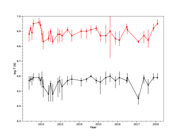
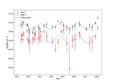
Figure 9: Time series of temperature (left panel) and emission measure (right panel) of the 2-T fits to the EPIC spectra of $\iota$ Hor. The pattern of the X-ray light curve fit is shown for comparison.

The EPIC spectra of each of the snapshot observations were fit in order to calculate the X-ray luminosity. The results of the fits were used to identify the origin of the cycle. A visual inspection of Fig. 9 suggests that the emission measure of the hot component is the most sensitive of the four variables ($\log T_{1,2}$ and $\log EM_{1,2}$) to the activity cycle (especially at the minima of 2014, 2015, and 2017). We correlated these variables with $L_{\rm X}$, showing that the correlation is more direct with the emission measure (correlation factor $r=0.82,0.68$, and probability value, respectively, with the cool and hot components) than with the temperatures ($r=0.26,0.56$, $p=0.15,0.00095$). The cycle is thus modulated by the amount of material in the corona.

Coronal abundances were also measured while fitting the EMD using the atomic models of APED, which are based on solar photospheric abundances by Anders & Grevesse (1989). We then updated them to the reference values of Asplund et al. (2009). Both are shown in Table $a$ for completeness, together with the $\iota$ Hor photospheric abundances. Several authors report photospheric abundances of $\iota$ Hor (Bond et al., 2006; Biazzo et al., 2012; Soto & Jenkins, 2018). The values for most elements are quite similar in the literature, although Bond et al. (2006) calculates a lower [Fe/H]$\sim$0.08. We compare our results with those of Gonzalez & Laws (2007), which cover the longest list of elements common to our list of coronal elements, including oxygen and carbon, those with largest first ionization potential (FIP) in the list (Fig. 5). Neither coronal nor photospheric abundances of $\iota$ Hor deviate substantially from solar photospheric values. We thus conclude that there are no effects related to FIP in the corona of this star.

3.3 UV variability

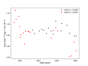
Figure 10: XMM-Newton/OM time series in the two UV filters. Data from UVM2 filter are multiplied $\times 0.9$ for a better display. No activity cycle is evident in the UV.

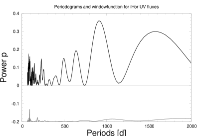
Figure 12: Generalized Lomb–Scargle power spectrum (top panel) and window function (bottom panel) of the long-term OM/UV light curve of $\iota$ Hor. The highest peak, with low significance, is at 909 d.

The UV measurements obtained with the XMM-Newton OM define a time series of the same length as the X-ray data (i.e., 7 years). The long-term UV light curve of $\iota$ Hor is displayed in Fig. 10. Some of the observations included measurements with both the UVM2 and the UVW2 filters. We used the flux ratio of the star in the two bands ($f_{\rm UVM2}/f_{\rm UVW2}\sim 0.9$) from these observations to scale down the UVM2 measurements for a better display of data from both UV filters in Fig. 10. The variation in the flux density is limited to $\sim$14% in the UVM2 filter and to only $\sim$4% in the UVW2 band. No periodic pattern is visible in the UV light curve. We calculated a periodogram with the GLS software, using the combined data of both filters. No significant periodicity is found (Fig. 12).

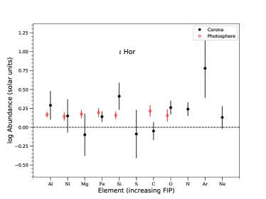
Figure 5: Coronal abundances (from XMM-Newton/RGS) and photospheric abundances (Gonzalez & Laws, 2007) of $\iota$ Hor in solar units, using Asplund et al. (2009) as reference.

3.4 Starspot modulation

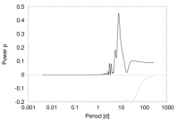
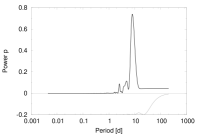
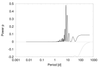
Figure 13: Generalized Lomb–Scargle power spectrum (top panels) and window function (bottom panels) for the TESS light curve of $\iota$ Hor in Sector 2 (left), Sector 3 (center), and combined data of sectors 2 and 3 (right). The highest peaks are at a period of $P_{\rm rot}=8.43$ d, 7.95 d, and 9.47 d, respectively.

We searched for the rotation period of $\iota$ Hor using the same GLS routine on the TESS light curve that we had applied to the X-ray time series in Sect. 3.1 First, we used GLS on each TESS sector individually. As this GLS implementation can only deal with up to 10000 data points we binned the data of each sector by a factor of 3. The highest peaks in the periodograms correspond to a rotation period of $8.43\pm 0.02$ d and $7.95\pm 0.02$ d for sectors 2 and 3, respectively (Fig. 13). Then we repeated the GLS analysis for the full TESS light curve (both sectors combined). The data had to be binned by a factor of 4. The periodogram clearly shows two significant peaks at $P_{\mathrm{1}}=7.718\pm 0.007$ d and $P_{\mathrm{2}}=9.47\pm 0.02$ d (Fig. 13). Our GLS analysis and the double-humped structure of the light curve suggest two dominating spots. As can be seen from Fig. 6 the morphology of the light curve changes from one rotational cycle to the next indicating spot evolution. The observed change in period between observations of Sectors 2 and 3 might be due to differential surface rotation combined with changes in the spot latitude. A quantitative assessment of this effect is beyond the scope of this work. We adopt the mean of the values ($P_{\mathrm{1}}$, $P_{\mathrm{2}}$) from each of the two sectors periodograms, $P_{\mathrm{rot}}=8.19\pm 0.26$ d.

To our knowledge, we have derived here the first photometric measurement of the rotation period for $\iota$ Hor. In Table 4 we compare our result to measurements presented previously in the literature based on different diagnostics. As can be seen, all these values cluster around $\approx 7.0-8.5$ d. However, the LS periodogram obtained from the TESS light curves provides a much higher significance than the other methods (see, e.g., Fig. 6 in Alvarado-Gómez et al., 2018b).

We combined the TESS measurement of $P_{\rm rot}$ with the published values for the projected rotational velocity ($v\sin{i}=6.0\pm 0.5$ km/s; Alvarado-Gómez et al., 2018b) and the stellar radius ($R=1.17\pm 0.04\,{\rm R_{\odot}}$, Fuhrmann et al., 2017), and we determined the inclination of $\iota$ Hor to be $i=56^{\circ}$ (range $49^{\circ}-65^{\circ}$ taking into account the uncertainties).

3.5 White-light flares

We also searched for flares in the TESS light curve of $\iota$ Hor. Our flare analysis procedure is based on the routine used in Stelzer et al. (2016). With an iterative process of boxcar smoothing of the light curve and removing $3\sigma$ outliers we created a final smoothed light curve, that was interpolated to all data points of the original input light curve. All points that lie $3\sigma$ above the final smoothed light curve were flagged. All groups of at least three consecutive flagged points were assigned as potential flares.

To validate potential flares as flare candidates, five criteria have to be fulfilled: (i) the flare does not happen right before or after a data gap, (ii) the maximum flux value is significant with at least $3\sigma$, (iii) the flux ratio between the flare maximum and the last flare point is $\geq$3, (iv) the difference between the second-to-last and the last flare point is smaller than the standard deviation of the cleaned light curve, and (v) a flare template suggested by Davenport et al. (2014) fits the data better than a linear fit through all flare points.

We could not detect any flares in the TESS light curve of $\iota$ Hor (i.e., there were no groups of at least three consecutive outlying points). Therefore, the flare validation procedure described in the previous paragraph could not be applied. We present it here because in Sect. A.1 we analyze flares in a comparison sample to evaluate the possibility of $\iota$ Hor hosting (rare) superflares.

Figure 6: Two-minute cadence light curve of $\iota$ Hor observed by TESS in 2018 September.

4 Discussion

The number of results obtained yield different topics to be discussed: the X-ray activity cycle, $\iota$ Hor and the early evolution of the solar corona, the observed pattern in the coronal abundances, the net UV emission coming from the chromosphere, and the analysis of $\iota$ Hor in the context of superflare stars.

4.1 X-ray activity cycle

The chromospheric behavior in Ca ii H&K was used to identify the activity cycle (Metcalfe et al., 2010), but later observations indicate a more erratic behavior of the chromospheric cycle in the period between 2013 and 2017, also resulting in a small amplitude of the S-index, as shown in Fig. 2. Alvarado-Gómez et al. (2018b) explain the observed behavior as the superposition of two periods of 1.97 and 1.41 yr of similar amplitudes. The origin of these two periods remains unclear.

The observed coronal cycle gives rise to an intriguing question: Why is the chromospheric cycle of $\iota$ Hor  substantially more irregular than its coronal counterpart? The combination of the chromospheric and coronal data initially pointed to a modulation of the 1.6 yr cycle with a longer term periodicity (SSM13, ; Sanz-Forcada & Stelzer, 2016). However, the inspection of the chromospheric and the coronal longer data set now available indicates that coronal cycle is quite regular in duration and amplitude, while the chromospheric cycle is irregular and seems to have faded since late 2013. A geometrical effect was suggested by SSM13 to explain the irregularities observed earlier in the chromospheric cycle, just before the X-ray monitoring started. With a stellar rotation axis inclination of $i\sim 56^{\circ}$ we might be biased towards viewing the activity in one of the hemispheres, but with irregularities introduced by the different visibility of the more occulted hemisphere. This effect should be less evident in X-rays, since X-ray emission originates in coronal material, more extended over the stellar photosphere, in addition to being optically thin. The observed behavior in $\iota$ Hor seems to support this idea.

4.2 $\iota$ Hor as a young solar analog

The RGS spectroscopic analysis reveals a very similar coronal structure to that of $\kappa$ Cet (G5V, $\log L_{\rm X}/L_{\rm bol}=-4.4$, Sanz-Forcada in prep.). Both have a similar age ($\sim 600$ Myr, Lachaume et al., 1999; SSM13, , and references therein) and can be considered a sort of proxy of the young Sun, given their solar-like spectral types. The age of both stars corresponds to the estimated solar age when the earliest known forms of life appeared on Earth (Cnossen et al., 2007). The coronal properties of $\iota$ Hor are of special interest to calibrate the effects of high-energy photons and particles on the early Earth. The stellar wind properties are expected to vary during the activity cycles (Oran et al., 2013; Alvarado-Gómez et al., 2016). Effects of the solar cycle on the Earth’s atmosphere include the variation of cosmic rays arriving to the atmosphere, the change in the size of the exosphere, or the thermosphere cooling fluctuations (e.g., Friis-Christensen & Lassen, 1991; Svensmark et al., 2016; Mlynczak et al., 2018). The influence of activity cycles could introduce a modulation in the atmosphere of the planet thorough these effects, although on a different scale from that detected on the Earth given the different length and amplitude of the cycle in $\iota$ Hor and the Sun. It has been proposed that activity cycles can also act as weather seasons for biological processes in exoplanets under some circumstances (Mullan & Bais, 2018).

4.3 Coronal abundances

Peretz et al. (2015) used the EPIC-pn spectrum to measure the coronal abundances of a few elements in $\iota$ Hor, which were then compared with the photospheric values in the literature. Our superb RGS combined spectrum allows for a more accurate measurement of the coronal abundances (Table $a$, Fig. 5). The comparison we make with the photosphere of $\iota$ Hor shows no trend related to the FIP. Our results differ from those of Peretz et al. (2015) who find an FIP effect (elements with low FIP are enhanced in the corona with respect to the photosphere) in $\iota$ Hor based on the [Fe/O] ratio. However, they calculate a very low oxygen coronal abundance, [O/H]=$-0.45\pm 0.05$, quite different from our value from EPIC ([O/H]=$-0.01\pm 0.03$) or RGS ([O/H]=$0.26\pm 0.10$) spectra. This discrepancy in the EPIC results with Peretz et al. (2015) could be due to our better statistics, which allow us to use a 3-T model to fit the spectrum, thus with a better sampling of the region where oxygen lines are formed. Our result also contradicts the conclusion made by Wood & Linsky (2010), followed by Laming (2015), in which FIP-related effects in dwarfs are correlated with spectral type, using only stars with $\log L_{\rm X}$(erg s^-1)$<29$. This would imply that $\iota$ Hor (G0V) would have an FIP effect, while M dwarfs would suffer an inverse FIP effect. The authors use solar photospheric values for their comparison in the dwarf M stars, instead of stellar photospheric abundances. In the case of GK dwarfs they use in the comparison the Mg and Si as low FIP elements rather than Fe, which is the low-FIP element with the best determined abundances. Finally, the exclusion of high-activity stars in the sample of the above-mentioned FIP studies sheds some doubts on whether the FIP (or inverse FIP) effect is related to spectral type or to stellar activity.

A question that remains open is whether the coronal abundances remain constant during the activity cycle. A recent work reveals that solar coronal abundances may vary along the activity cycle (Brooks et al., 2017). The quality of our data does not allow us to search for variations in the abundances between the different observations, an exercise that would be reliable only with high resolution (RGS-like) spectra with enough statistics.

4.4 UV chromospheric emission

For late-type stars the observed UV flux is a combination of photospheric and chromospheric contributions. To examine what fraction of the UV emission measured by the OM is from the chromosphere of $\iota$ Hor, we calculated the chromospheric excess flux density ($F_{\rm UV,exc}$) as the difference between the UV observed flux density and the photospheric flux density ($F_{\rm sy}$) predicted by atmosphere models for the respective UV waveband (i.e., $F_{\rm UV,exc}=F_{\rm UV}-F_{\rm sy}$). We carried out this analysis for the two filters of the XMM-Newton OM used during our campaigns and for published GALEX measurements (Shkolnik, 2013). The GALEX near ultraviolet filter (NUV) observation was discarded because $\iota$ Hor was saturated according to the detector limits reported by Morrissey et al. (2007).

In order to determine the expected photospheric flux, we first extracted all the published photometric data of $\iota$ Hor from the catalogs in VizieR. Using the online tool Virtual Observatory SED Analyzer (VOSA; Bayo et al., 2008) we then fit these data with the model BT-Settl-CIFIST (Allard, 2014; Baraffe et al., 2015). As input parameters the SED fitting procedure requires the effective temperature ($T_{\rm eff}$), the logarithm of the surface gravity ($\log g$), and the metallicity. We fixed the gravity and the metallicity values to $\log g=4.5$ and [Fe/H]$=0$. These are the values in the spectral grid that are the closest to the literature values for $\iota$ Hor according to Fuhrmann et al. (2017). In the best fit we obtained $T_{\rm eff}=6000\pm 50$ K, consistent with the effective temperature given by Fuhrmann et al. (2017). We then calculated the photospheric flux density as $F_{\rm sy}=\int F_{\rm mod}(\lambda)T_{\rm filter}(\lambda)d\lambda$. Here, $F_{\rm mod}(\lambda)$ is the flux density of the synthetic BT-Settl-CIFIST spectrum, with $T_{\rm eff}$ equal to the best-fit parameter $6000$ K, and $T_{\rm filter}(\lambda)$ is the normalized transmission curve of the respective UV filter. Since the synthetic spectrum is available in terms of surface flux density, we used $R_{\ast}=1.17$ and stellar distance to get the flux density at Earth.

In Table $a$ we provide the observed and the excess flux densities for the three UV filters with reliable data. The errors stated in Table $a$ were propagated from the dilution factor $\left(R_{\ast}/D\right)^{2}$. The results show an expected increase in the chromospheric excess for decreasing wavelengths. Finally, the chromospheric far-ultraviolet (FUV) excess of $\iota$ Hor, $L_{\rm FUV,exc}$= $(1.140\pm 0.005)\times 10^{29}$ erg s^-1, is consistent with the relation between X-rays and FUV chromospheric emission reported in Pizzocaro et al. (2019).

4.5 Photometric activity

One result of the analysis of the photometric data collected by NASA’s Kepler mission was the detection of flare activity on solar-like stars, which before had rarely been seen. A number of these stars show flares with energies more than ten times larger than the largest known solar event ($10^{32}$ erg). The Kepler data revealed hundreds of sun-like stars with these so-called “superflares” (e.g., Maehara et al., 2012; Notsu et al., 2013; Shibayama et al., 2013). In a theoretical work Airapetian et al. (2016) concluded that superflares, and the coronal mass ejections associated with them, could serve as a potential catalyst for the origin of life on the early Earth. Karoff et al. (2016) explored the relation between superflare stars and their chromospheric emission for a sample of stars with $T_{\rm eff}=5100-6000$ K. In that work the distribution of stars with superflares peaks at a Ca ii H&K S-index $\sim 0.26$, well above the stars with no flares ($\sim 0.19$). According to this distribution $\iota$ Hor is a good candidate to be a superflare star.

As described in Sect. 3.5, in our analysis of the TESS data of $\iota$ Hor we could not find any flare events, but since the data span in total only an observing time of $\sim$52 d, we wanted to test the hypothesis of $\iota$ Hor being a superflare star, comparing it with a sample of Kepler superflare stars. If $\iota$ Hor had a flare rate similar to that of the stars in our Kepler sample ($0.03-0.23\,{\rm N_{\rm flares}/day}$; see Appendix A.1) we would expect to detect between $1.4$ and $11.1$ (average: $3.8$) flares in the $\sim 48$ d of actual TESS observations. To quantify the probability of no flaring events during the TESS observations of $\iota$ Hor, we simulated the incidence of flares in a putative observing time span of $t_{\rm obs}=1$ Myr. Using the average flare rate $0.08\,{\rm N_{Flares}/day}$ of our Kepler sample (see Sect. A.1) and assuming this flare rate to be constant for the whole $t_{\rm obs}$, we obtained $29.2\times 10^{6}$ flares, which we randomly injected at times between $t=0$ and $t_{\rm obs}$. Then we measured the time lags, $\delta t$, between consecutive flares. Finally, we calculated the fraction of all $\delta t$ that are larger than the duration of $\iota$ Hor’s TESS light curve. We found that the probability of no flares being observed in the time spanned ($52.1$ d) is $1.55$%. If we also consider the gap of $4.4$ d between sectors 2 and 3 where possible flares could go unnoticed, the probability for zero flares in the observed light curve increases to $2.20$%. There is, therefore, a small probability that $\iota$ Hor is a superflare star, but no such event has been discovered yet. We also note that our estimate ignores that the sensitivity for flare detection is probably somewhat lower for TESS with respect to Kepler as a result of its redder bandpass ($\lambda\lambda 6000-10000\AA$ vs $\lambda\lambda 4200-8800\AA$).

5 Conclusions

The X-ray observations of $\iota$ Hor confirm a robust coronal cycle of $P=588.5\pm 5.5$ d, with an amplitude of 2.3 in the 0.12-2.48 keV X-ray band. The coronal cycle is modulated by the amount of loops present in the corona. The effective temperature and age of this star make it a good representation of the Sun at an age of $\sim 600$ Myr, when life appeared on Earth. The understanding of the high-energy properties of such young solar analogs is thus of paramount importance for assessing the variable irradiation to which a proto-Earth is exposed. Chromospheric cycles show a direct relation between rotation and cycle periods. The X-ray (coronal) cycle comparison between the “early Sun” ($\iota$ Hor) and the present-day Sun reveal that cycles in the more evolved state are longer in duration than cycles of the younger Sun, but they also have a larger amplitude in X-rays. It is expected that the influence of the X-ray cycle in the atmosphere of planets is also greater now. Given the short duration of early cycles, we can speculate that their effects mimic seasonal weather patterns for biological processes, as proposed by Mullan & Bais (2018).

The X-ray observations of $\iota$ Hor cover four complete and consecutive coronal cycles, more than observed on the Sun. This has allowed us to study cycle-to-cycle variability, and we noticed an irregular behavior of the chromospheric signal, but a more regular coronal modulation. We propose that this disagreement is due to a geometrical effect. Given the inclination of $\sim 56^{\circ}$ (see below) we do not observe in a symmetric view the northern and southern hemispheres of the star. While this may have some effects on the chromospheric emission depending on the spot coverage of each hemisphere, which may be out of phase, the coronal signal comes from more extended material and should be less sensitive to viewing effects.

The spectroscopic analysis of the corona of $\iota$ Hor shows a medium activity level star with an abundance pattern similar to the solar photosphere, with no FIP-related effects. This pattern contradicts the earlier results measured in the literature using low-resolution X-ray spectra. It also breaks the dependence of the FIP effect with spectral type proposed by Wood & Linsky (2010).

Table 4: Rotation period estimates for $\iota$ Hor.

$P_{\rm rot}$ (d)	diagnostic	reference
$8.19\pm 0.26$	photometric time series	this work
$7.7$	S-index	(1)
$7.88$	longitudinal field	(1)
$7.03$	radial velocity	(1)
$7.9$	chromospheric activity	(2)
$7.9-8.5$	S-index	(3)
$7.9-8.4$	radial velocity	(4)

Table 5: Observed UV flux densities and chromospheric excess

Filter	$\lambda_{\rm eff}$	$f_{\rm\lambda,obs}$	$f_{\rm\lambda,exc}$
	($\AA$)	(erg s-1 cm${}^{-2}\AA^{-1}$)	(%)
GALEX/FUV	$1516$	$(1.29\pm 0.03)\times 10^{-14}$	$71\pm 3$
OM/UVW2	$2120$	$(1.67\pm 0.01)\times 10^{-12}$	$39\pm 4$
OM/UVM2	$2310$	$(1.84\pm 0.06)\times 10^{-12}$	$20\pm 7$

We have presented the first photometric measurement of the rotation period for $\iota$ Hor using TESS data. Our value is consistent with earlier measurements from spectroscopic data (e.g., S-index, radial velocity, longitudinal magnetic field). Combining our value for $P_{\rm rot}$ ($8.19\pm 0.26$ d) with historical measurements of $v\sin{i}$ and stellar radius, we derived a new estimate for the inclination, $i=56^{\circ}$. No white-light flares are detected in the TESS light curve, but our evaluation of the flare amplitudes of Kepler superflare stars has shown that the possibility of occasional superflares on $\iota$ Hor cannot be excluded. Superflares would likely have strong effects on the early atmosphere of the Earth, especial if they yielded coronal mass ejections (but see Alvarado-Gómez et al., 2018a, and references therein).

The UV emission does not follow the cyclic behavior detected in the X-ray light curve, and its variability amplitude is limited to $\sim 14$% at most. We used the UV spectral energy distribution to quantify for the first time the chromospheric broadband UV flux of $\iota$ Hor, after subtracting the photospheric contribution to the SED.

The multi-wavelength study of long-term variability in other stars of similar or younger age will tell us how general the case of $\iota$ Hor is, and whether it is the age of the first activity cycles in stars like the Sun. The study of coronal cycles in other stars at different ages is also of interest to understand how the amplitude of the X-rays emission in the cycle evolves with stellar age.

Appendix A Supplementary material

Table 6: XMM-Newton/RGS line fluxes of $\iota$ Hor^a

Ion	$\lambda_{\rm model}$ (Å)	$\log T_{\rm max}$	$F_{\rm obs}$	$S/N$	Ratio	Blends
Mg xii	8.4192	7.1	1.18e-15	3.4	-0.36	Mg xii 8.4246
Mg xi	9.1687	6.9	1.16e-14	11.9	0.24	Mg xi 9.2312
Mg xi	9.3143	6.9	2.27e-15	5.3	-0.13
Ne x	10.2385	6.9	3.52e-15	7.3	0.18	Ne x 10.2396
Fe xvii	10.5040	6.9	1.13e-15	4.3	-0.32	Fe xviii 10.5364, 10.5382, 10.5640
Fe xvii	10.6570	6.9	9.45e-16	4.0	-0.44	Fe xix 10.6001, 10.6116, 10.6193, 10.6840, Ne ix 10.6426
Ne ix	11.0010	6.7	1.32e-15	4.9	-0.17	Fe xxiii 10.9810, 11.0190, Na x 11.0026, Fe xvii 11.0260
Fe xvii	11.1310	6.9	1.54e-15	5.3	-0.27
Fe xvii	11.2540	6.9	3.60e-15	8.2	-0.07
Fe xviii	11.4230	7.0	2.55e-15	6.9	0.01	Fe xviii 11.4226, 11.4254, 11.4274, Fe xvii 11.4383
Ne ix	11.5440	6.7	1.47e-15	5.3	-0.43	Fe xviii 11.5270, Ni xix 11.5390
Fe xxii	11.7700	7.2	2.97e-15	7.7	0.17	Fe xxiii 11.7360, Ni xx 11.8320, 11.8460
Ne x	12.1321	6.9	1.84e-14	19.7	-0.12	Fe xvii 12.1240, Ne x 12.1375
Fe xxi	12.2840	7.2	1.18e-14	15.9	0.06	Fe xvii 12.2660
Ni xix	12.4350	7.0	5.43e-15	10.9	-0.03	Fe xxi 12.3930, Fe xvi 12.3973, 12.3983
Fe xvi	12.5399	6.8	1.13e-15	5.0	-0.22	Fe xx 12.5260, 12.5760, 12.5760, Fe xvii 12.5391
Ni xix	12.6560	7.0	4.92e-16	3.3	-0.32	Fe xxi 12.6490
Fe xvii	12.6950	6.9	8.47e-16	4.3	0.09
Fe xx	12.8460	7.1	4.72e-15	10.3	-0.01	Fe xxi 12.8220, Fe xx 12.8240, 12.8640, Fe xviii 12.8430
Fe xx	12.9120	7.1	4.22e-15	9.6	0.10	Fe xix 12.9033, 12.9330, 13.0220, Fe xx 12.9650
Fe xx	13.2740	7.1	9.26e-16	4.6	-0.09	Fe xix 13.2261, 13.2933, Fe xxii 13.2360, Fe xx 13.2453, 13.2932, Ni xx 13.2560
Fe xviii	13.3230	7.0	2.24e-15	7.2	-0.16	Ni xx 13.3090, Fe xviii 13.3550, 13.3807, Fe xx 13.3850
Ne ix	13.4473	6.7	1.61e-14	19.6	0.04	Fe xix 13.4620, 13.4970
Fe xix	13.5180	7.1	1.10e-14	16.3	0.18	Ne ix 13.5531
Ne ix	13.6990	6.7	9.03e-15	14.7	0.04	Fe xix 13.6450, 13.6878, 13.7054
Fe xvii	13.8250	6.9	1.96e-14	21.9	0.21	Ni xix 13.7790, Fe xix 13.7950, Fe xvii 13.8920
Fe xviii	13.9530	7.0	2.05e-15	7.1	0.05	Fe xix 13.9263, 13.9330, Fe xx 13.9620
Ni xix	14.0430	7.0	6.74e-15	12.8	0.13	Fe xxi 14.0080, Fe xix 14.0340, 14.0388, Ni xix 14.0770
Fe xviii	14.1580	7.0	3.72e-15	9.5	0.55	Fe xix 14.1272, 14.1429, 14.1487, 14.1496, Fe xviii 14.1348
Fe xviii	14.2080	7.0	2.65e-14	25.5	-0.01	Fe xviii 14.2560
Fe xviii	14.3730	7.0	1.11e-14	16.4	-0.09	Fe xviii 14.3430, 14.3990, 14.4250, 14.4555
Fe xviii	14.5340	7.0	9.28e-15	15.2	0.05	Fe xviii 14.5608,14.5710
Fe xix	14.6640	7.1	2.07e-15	7.2	-0.28	Fe xviii 14.6160, 14.6566, 14.6887, O viii 14.6343, 14.6344
Fe xvii	15.0140	6.9	1.15e-13	54.1	0.20
O viii	15.1760	6.6	8.45e-15	14.5	0.16	Fe xvi 15.1629, O viii 15.1765, Fe xix 15.1980
Fe xvii	15.2610	6.9	5.04e-14	35.7	0.40
Fe xvii	15.4530	6.8	1.58e-14	25.4	0.23	Fe xviii 15.3539, 15.4940, Fe xvi 15.4955
Fe xviii	15.6250	7.0	5.41e-15	11.8	-0.12	Fe xvi 15.6398
Fe xviii	15.7590	7.0	2.56e-15	8.1	0.40	Fe xvi 15.7389
Fe xviii	15.8240	7.0	3.47e-15	9.4	-0.28	Fe xviii 15.8700
O viii	16.0055	6.6	1.56e-14	20.1	-0.07	Fe xviii 15.9310, 16.0040, Fe xvii 15.9956, O viii 16.0067
Fe xviii	16.0710	7.0	1.80e-14	21.6	0.03	Fe xviii 16.0450, 16.1590, Fe xix 16.1100
Fe xvii	16.3500	6.9	3.46e-15	9.4	-0.07	Fe xvii 16.2285, Fe xix 16.2830, 16.2857, Fe xviii 16.3200
Fe xvii	16.7800	6.8	4.97e-14	35.9	0.12
Fe xvii	17.0510	6.8	1.58e-13	63.9	0.24	Fe xvii 17.0960
O vii	17.3960	6.5	2.93e-15	8.6	0.43	Fe xvi 17.4100, 17.4982, Cr xvi 17.4207, 17.4252
Fe xviii	17.6230	7.0	3.78e-15	9.9	-0.20
O vii	18.6270	6.4	2.82e-15	8.5	-0.06	Ca xviii 18.6909
O viii	18.9671	6.6	5.94e-14	39.1	0.01	O viii 18.9725
N vii	20.9095	6.4	8.89e-16	4.5	0.05	N vii 20.9106
Ca xvii	21.1560	6.9	1.90e-15	6.7	-0.02
O vii	21.6015	6.4	1.93e-14	21.1	0.07
O vii	21.8036	6.4	3.40e-15	8.7	0.13
O vii	22.0977	6.4	1.29e-14	17.0	0.01	Ca xvii 22.1467
S xiv	24.2000	6.7	5.07e-16	3.5	-0.23	Ca xvi 24.2214, Ca xv 24.2344, Ca xiv 24.2599, S xiv 24.2850
N vii	24.7792	6.4	7.53e-15	13.5	-0.01	Ar xv 24.7366, 24.7400, N vii 24.7846, Ar xvi 24.8509
Ar xvi	25.6844	6.8	8.33e-16	4.2	-0.09	Ca xiv 25.7299, 25.7330
Ar xii	31.3030	6.5	1.08e-15	3.9	0.47	Fe xviii 31.3157
S xiv	33.5490	6.6	8.56e-16	3.3	0.22	Si xi 33.5301, Fe xviii 33.5387
C vi	33.7342	6.2	5.42e-15	8.4	0.02	C vi 33.7396
Fe xvii	35.6844	6.9	2.67e-15	5.7	0.53	Ar xiii 35.7285, Fe xvi 35.7291, Ca xi 35.7370

^a Line fluxes (in erg cm^-2 s^-1) measured in XMM-Newton/RGS $\iota$ Hor spectra, and corrected by the ISM absorption. log $T_{\rm max}$ (K) indicates the maximum temperature of formation of the line (unweighted by the EMD). “Ratio” is the log($F_{\mathrm{obs}}$/$F_{\mathrm{pred}}$) of the line. Blends amounting to more than 5% of the total flux for each line are indicated.

Table 7: HST/STIS line fluxes of $\iota$ Hor^a

Ion	$\lambda_{\rm model}$ (Å)	$\log T_{\rm max}$	$F_{\rm obs}$	$S/N$	Ratio	Blends
Si iii	1206.5019	4.9	1.11e-13	9.5	-0.44
O v	1218.3440	5.5	1.37e-14	7.4	-0.01
N v	1238.8218	5.4	1.59e-14	7.8	0.02
N v	1242.8042	5.4	6.94e-15	5.2	-0.03
Si ii	1264.7400	4.5	8.82e-15	5.6	0.26
Si ii	1265.0040	4.6	2.55e-15	5.1	-0.11
Si iii	1298.9480	4.9	3.55e-15	7.5	0.81
Si ii	1309.2770	4.6	3.56e-15	5.3	0.01
C ii	1334.5350	4.7	3.56e-14	12.5	-0.29
C ii	1335.7100	4.7	7.38e-14	16.6	0.22	C ii 1335.665
Si iv	1393.7552	5.0	6.18e-14	23.6	0.23
Si iv	1402.7704	5.0	3.18e-14	11.3	0.24
Si ii	1526.7090	4.5	1.02e-14	8.0	0.35
Si ii	1533.4320	4.5	1.62e-14	3.8	0.26
C iv	1548.1871	5.1	1.04e-13	13.1	0.03
C iv	1550.7723	5.1	4.95e-14	13.7	0.01
Al ii	1670.7870	4.6	2.43e-14	5.3	-0.01

^a Line fluxes (in erg cm^-2 s^-1) measured in HST/STIS $\iota$ Hor spectra, and corrected for the ISM absorption. Columns as in Table 6

A.1 Determination of flare rate for solar-like Kepler superflare stars

Since we could not find any flare events in the $\sim$52 d spanned by the TESS data of $\iota$ Hor (the data actually cover only 48 d), we wanted to test the hypothesis that $\iota$ Hor is a superflare star. To this end we carried out a comparison with a sample of Kepler superflare stars. From the sample of Balona (2015) we selected stars with $T_{\rm eff}=5800-6200$ K and $P_{\rm rot}=5-15$ d that have shown at least one flare with energy $>10^{34}$ erg in the Kepler short-cadence data ($\iota$ Hor TESS observations have a two-minute cadence). We found seven stars that fulfilled these selection criteria.

The short-cadence light curves of this Kepler flare star sample were downloaded from the MAST Portal. For the analysis we considered simple aperture photometry (SAP) fluxes. Six out of seven targets were observed in short-cadence mode only for $1/3$ of an observing quarter. The short-cadence light curves of one Kepler observing quarter are split into three parts (i.e., for $\sim$30 d). Only KIC 12004971 has short-cadence data for two full quarters (quarter 15 and 17) and for an additional $1/3$ of the time in quarter 1.

The flare analysis following the procedure outlined in Sect. 2.3 was performed individually for all $1/3$ of a quarter. The results are given in Table 8. In total we found 27 flares for the seven Kepler targets in 12 pieces of $1/3$ quarter. Figure 14 shows the histogram of the detected flare amplitudes. The flare amplitude is measured as the difference between the observed peak flux and the quiescent flux represented by the light curve from which rotational signal and outliers were removed (see Sect. 3.5 and Stelzer et al., 2016). To show this result in absolute quantities we converted the relative values of the peak flare amplitude to an amplitude in terms of luminosity. The TESS and Kepler photometries are not flux calibrated. However, by assuming that the TESS and Kepler magnitudes correspond to the quiescent emission of the star, we could convert the $T_{\rm mag}$ (from the TESS candidate target list CTL v7.02 Stassun et al., 2018) and $K_{\rm p}$ (from the Kepler Input Catalog, KIC Kepler Mission Team, 2009) to flux using the zero-points and effective wavelengths provided at the filter profile service of the Spanish Virtual Observatory (SVO, Rodrigo et al., 2012). Then we applied the distances given in Sect. 1 for $\iota$ Hor, and in the CTL for the Kepler sample, to obtain the quiescent luminosity. The flare amplitude is then converted to a luminosity by multiplying the quiescent luminosity by the relative value of the peak flare amplitude.

The red solid line in Fig. 14 indicates the flare detection threshold for $\iota$ Hor. All flares that we found in the Kepler sample would have been easily detected in the $\iota$ Hor TESS light curve. However, the flare detection threshold for the Kepler stars is on average 2.3 times (0.36 dex in log scale) higher than that for the TESS observation of $\iota$ Hor.

The individual flare rates of the stars in our Kepler sample range from $0.03\,{\rm N_{Flares}/day}$ to $0.23\,{\rm N_{Flares}/day}$ with an average of $0.08\,{\rm N_{Flares}/day}$. This latter value is used in Sect. 4.5 to determine the probability of $\iota$ Hor being a superflare star despite the absence of such events in the TESS light curve.

Table 8: Summary of the properties of our Kepler superflare star sample

KIC	$T_{\mathrm{eff}}$	$P_{\mathrm{rot}}$	Quarter	duration	$N_{\mathrm{Flares}}$	$N_{\mathrm{Flares}}$/day
	(K)	(d)		(d)
1025986	5966	10.076	03	30.03	7	0.23
6786176	5836	7.992	04	31.05	2	0.06
7880490	6116	7.377	03	30.03	6	0.20
8556311	5886	10.222	02	29.97	1	0.03
9752973	5865	13.500	03	30.34	2	0.07
12004971	5811	6.686	01	33.49	1	0.03
			15	30.83	1	0.03
			15	30.09	0	0
			15	34.91	5	0.14
			17	22.37	1	0.04
			17	4.21	0	0
12072958	5929	5.107	04	31.05	1	0.03
					$\varSigma$ 27	Ø 0.08

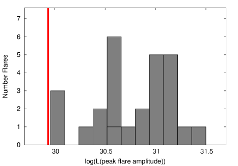
Figure 14: Histogram of the luminosity at the peak emission for the detected flares in the Kepler superflare star sample. The red solid line indicates the flare detection threshold in the TESS observation of $\iota$ Hor.