Magnetic field, activity and companions of V410 Tau

Abstract

We report the analysis, conducted as part of the MaTYSSE programme, of a spectropolarimetric monitoring of the $\sim$0.8 Myr, $\sim$1.4 ${\rm M}_{\odot}$ disc-less weak-line T Tauri star V410 Tau with the ESPaDOnS instrument at the Canada-France-Hawaii Telescope and NARVAL at the Télescope Bernard Lyot, between 2008 and 2016. With Zeeman-Doppler Imaging, we reconstruct the surface brightness and magnetic field of V410 Tau, and show that the star is heavily spotted and possesses a $\sim$550 G relatively toroidal magnetic field.

We find that V410 Tau features a weak level of surface differential rotation between the equator and pole $\sim$5 times weaker than the solar differential rotation. The spectropolarimetric data exhibit intrinsic variability, beyond differential rotation, which points towards a dynamo-generated field rather than a fossil field. Long-term variations in the photometric data suggest that spots appear at increasing latitudes over the span of our dataset, implying that, if V410 Tau has a magnetic cycle, it would have a period of more than 8 years.

Having derived raw radial velocities (RVs) from our spectra, we filter out the stellar activity jitter, modeled either from our Doppler maps or using Gaussian Process Regression. Thus filtered, our RVs exclude the presence of a hot Jupiter-mass companion below $\sim$0.1 au, which is suggestive that hot Jupiter formation may be inhibited by the early depletion of the circumstellar disc, which for V410 Tau may have been caused by the close (few tens of au) M dwarf stellar companion.

1 Introduction

Investigating the birth and youth of low-mass stars ($<3$ ${\rm M}_{\odot}$) and of their planetary systems heavily contributes to unveiling the origin and history of the Sun and of its planets, in particular the life-hosting Earth. We know that stars and their planets form from the collapse of parsec-sized molecular clouds which progressively flatten into massive accretion discs, until finally settling as pre-main-sequence (PMS) stars surrounded by protoplanetary discs. T Tauri stars (TTSs) are PMS stars that have emerged from their dust cocoons and are gravitationally contracting towards the main sequence (MS); typically aged 1-15 Myr, they are classical TTSs (cTTSs) when they are still surrounded by a massive accretion disc (where planets are potentially forming), and weak-line TTSs (wTTSs) when their accretion has stopped and their inner disc has dissipated. Large-scale magnetic fields are known to play a crucial role in the early life of low-mass stars, as they can open a magnetospheric gap at the center of the disc, funnel accreting disc material onto the star, induce stellar winds and prominences, and thus impact the angular momentum evolution of TTSs (Donati & Landstreet, 2009). Observing and understanding the magnetic topologies of TTSs is therefore a necessary endeavour to complete our understanding of stellar and planetary formation (e.g. Bouvier et al., 2007).

Since the first detection of a magnetic field around a cTTS nearly 20 years ago (Johns-Krull et al., 1999), the large-scale topologies of a dozen cTTSs were mapped (e.g. Donati et al., 2007; Hussain et al., 2009; Donati et al., 2010a, 2013) thanks to the MaPP (Magnetic Protostars and Planets) Large Observing Programme allocated on the 3.6 m Canada-France-Hawaii Telescope (CFHT) with the ESPaDOnS (Echelle SpectroPolarimetric Device for the Observation of Stars) high-resolution spectropolarimeter, using Zeeman-Doppler Imaging (ZDI), a tomography technique designed for imaging the brightness features and magnetic topologies at the surfaces of active stars (eg Brown et al., 1991; Donati & Brown, 1997). This first exploration showed that the topologies of cTTSs are either quite simple or rather complex depending on whether the stars are fully convective or largely radiative respectively (Gregory et al., 2012; Donati et al., 2013). Moreover, these fields are reported to vary with time (e.g. Donati et al., 2011, 2012, 2013) and resemble those of mature stars with similar internal structure (e.g. Morin et al., 2008), suggesting that they are produced through dynamo processes within the bulk of the convective zone.

The MaTYSSE (Magnetic Topologies of Young Stars and the Survival of close-in giant Exoplanets) Large Programme aims at mapping the large-scale magnetic topologies of $\sim$35 wTTSs, comparing them to those of cTTSs and MS stars, and probing the potential presence of massive close-in exoplanets (hot Jupiters/hJs) around its targets. It was allocated at CFHT over semesters 2013a to 2016b (510 h) with complementary observations from the ESPaDOnS twin NARVAL on the Télescope Bernard Lyot (TBL) at Pic du Midi in France and from the HARPS spectropolarimeter at the ESO Telescope at La Silla in Chile. Up to now, about a dozen wTTSs were studied with MaTYSSE for their magnetic topologies and activity, for example V410 Tau (Skelly et al., 2010), LkCa 4 (Donati et al., 2014) and V830 Tau (Donati et al., 2017). These studies showed that the fields of wTTSs are much more diverse than those of cTTSs, with for example V410 Tau and LkCa 4 displaying strong toroidal components despite being fully convective, as opposed to the results obtained on cTTSs (see discussion in Donati et al., 2014). MaTYSSE fostered the detection of two hJs around wTTSs, the 2 Myr-old V830 Tau b (Donati et al., 2016, 2017) and the 17 Myr-old TAP 26 b (Yu et al., 2017).

This new study focuses on V410 Tau, a very young ($\sim$1 Myr in Skelly et al., 2010) disc-less wTTS (Luhman et al., 2010) with a well-constrained rotation period of 1.872 d (Stelzer et al., 2003). One of the most observed wTTSs, V410 Tau has been the target of both photometric and spectropolarimetric observation campaigns. High variability detected in its light curve (Bouvier & Bertout, 1989; Sokoloff et al., 2008; Grankin et al., 2008) indicates a high level of activity, confirmed with Doppler maps (Skelly et al., 2010; Rice et al., 2011; Carroll et al., 2012) showing that the photosphere features large polar and equatorial cool spots, responsible for these modulations. Magnetic maps made by Skelly et al. (2010) and Carroll et al. (2012) have shown a highly toroidal and non-axisymmetric large-scale field despite the mostly convective structure of V410 Tau.

We first describe our data, comprising new NARVAL data from MaTYSSE added to previous spectropolarimetric data taken with ESPaDOnS and NARVAL in 2008-2011, and contemporaneous photometric observations taken at the Crimean Astronomical Observatory (CrAO) and from the Super Wide Angle Search for Planets (SuperWASP) campaign (Section 2). We then derive the general properties of V410 Tau (Section 3), after which we pursue the investigation of both its photosphere and its magnetic field, using ZDI with a model including both bright plages and cool spots (Section 4). Then, we disentangle the activity jitter from the actual radial velocities (RVs) in the RV curve, using models from our ZDI maps and Gaussian Process Regression (GPR), in order to look for a potential planet signature (Section 5), before finally discussing our results and concluding (Section 6).

2 Observations

Our spectropolarimetric data set spans from 2008 Oct to 2016 Jan, totalling 144 high-resolution optical spectra, both unpolarized (Stokes $I$) and circularly polarized (Stokes $V$). It is composed of 8 runs, most of which cover around 15 days, taken during 4 different seasons: 2008b-2009a, 2011a, 2013b and 2015b-2016a. The full journal of observations is available in Table 7. The 2008b data set and 4 points in the 2009a data set were taken with the ESPaDOnS echelle spectropolarimeter at CFHT, while the rest were taken with the ESPaDOnS twin NARVAL installed at TBL.

The raw frames are processed with the nominal reduction package Libre Esprit as described in e.g. Donati et al. (1997); Donati et al. (2011), yielding a typical root-mean-square (rms) RV precision of 20-30 m s^-1(Moutou et al., 2007; Donati et al., 2008). The peak signal-to-noise ratios (S/N, per 2.6 km s^-1 velocity bin) reached on the spectra range between 82 and 238 for the majority (3 spectra have a S/N lower than 70 and were rejected for ZDI and the RV analysis), with a median of 140.

Time is counted in units of stellar rotation, using the same reference date and rotation period as in Skelly et al. (2010), namely ${\mbox{BJD}_{0}=2,454,832.58033}$ and ${\hbox{$P_{\rm rot}$}=1.871970\pm 0.000010}$ d (Stelzer et al., 2003) respectively:

$$c=(\mbox{BJD}-\mbox{BJD}_{0})/\hbox{$P_{\rm rot}$}.$$ (1)

The stellar phase is defined as the decimal part of the cycle $c$.

The emission core of the Ca ii infrared triplet (IRT) presents an average equivalent width (EW) of $\simeq$13 km s^-1 (0.37 Å). The He i $D_{3}$ line is relatively weak with an average EW of 13 km s^-1 as well (0.25 Å), in agreement with the non-accreting status of V410 Tau. The H${\alpha}$ line has an average EW of 14 km s^-1 (0.33 Å) and a rms EW of 27 km s^-1 and exhibits a periodicity of period $1.8720\pm 0.0009$ d (see Appendix C). From the He i $D_{3}$ line, we detected small flares on 2008 Dec 10 (rotational cycle -15+3.514, as per Table 7), on the night of 2013 Dec 08 to 2013 Dec 09 (rotational cycles 959+4.090 and 959+4.151), and on the night of 2016 Jan 20 (rotational cycles 1376+0.021 and 1376+0.040). One big flare, on 2008 Dec 15 (rotational cycle -15+6.181), was visible not only in He i $D_{3}$ (EW $\simeq 30$ km s^-1) but also in H${\alpha}$ (EW $\simeq 230$ km s^-1) and the Ca ii IRT (core emission EW $\simeq 40$ km s^-1). We removed the 6 flare-subjected observations from our data sets in order to proceed with the mapping of the photosphere and surface magnetic field, as well as the RV analysis.

Least-squares deconvolution (LSD, see Donati et al., 1997) was applied to all our spectra in order to add up information from all spectral lines and boost the resulting S/N of both Stokes I and V LSD profiles. The spectral mask we employed for LSD was computed from an Atlas9 LTE model atmosphere (Kurucz, 1993) featuring $T_{\rm eff}$=4,500 K and $\log g$=3.5, and involves about 7 800 spectral features (with about 40 % from Fe i, see e.g. Donati et al., 2010b, for more details). Stokes $I$ and Stokes $V$ LSD profiles shown in Section 4 display distorsions that betray the stellar activity with a periodicity corresponding to the rotation of the star. Moonlight pollution, which affects 15 of our Stokes $I$ LSD profiles, was filtered out using a two-step tomographic imaging process described in Donati et al. (2016). The S/N in the Stokes $I$ LSD profiles, ranging from 1633 to 2930 (per 1.8 km s^-1 velocity bin) with a median of 2410, is measured from continuum intervals, including not only the noise from photon statistics, but also the (often dominant) noise introduced by LSD (see Table 7). The S/N in Stokes $V$ LSD profiles, dominated by photon statistics, range from 1817 to 6970 with a median value of 3584.

Phase coverage is of varying quality depending on the observation epoch. The 2008b data set, with only 6 points, covers only half the surface of the star (phases -0.20 to 0.30). The 2009a data set, although the densest with 48 points in 16 days and including data from both instruments, lacks observations between phases 0.05 and 0.20. The 2011a data set presents a large gap between phases -0.05 and 0.15, and a smaller one between phases 0.65 and 0.80. The 2013b and 2015b data sets are well sampled, and the 2016a data set, with only 9 points, lacks observations between phases 0.25 to 0.45 and -0.15 to 0.05.

Contemporaneous BVR_JI_J photometric measurements, documented in Table 8, were taken from the Crimean Astrophysical Observatory 1.25 m and 0.60 m telescopes between August 2008 and March 2017, counting 420 observations distributed over 9 runs at a rate of one run per year, each run covering 3 to 7 months. In each run, the visible magnitude presents modulations of a period $\sim$1.87 d and amplitude varying from 0.04 to 0.24 mag (see Appendix B). The visible magnitude reaches a global minimum of 10.563 during the 2014b run. We also used 2703 data points of visible magnitude from the Wide Angle Search for Planets (WASP Pollacco et al., 2006) photometric campaign covering semesters 2010b-2011a. Plots of the photometric data contemporaneous to our spectropolarimetric runs (i.e. 2008b+2009a, 2010b+2011a, 2013b+2014a and 2015b+2016a) are visible in Section 4.

3 Evolutionary status of V410 Tau

V410 Tau is a very well-observed three-star system located in the Taurus constellation at ${d=129.0\pm 0.5}$ pc from Earth (Galli et al., 2018, we chose this value over the Gaia result, ${130.4\pm 0.9}$ pc, because it is both in agreement with it and more precise). V410 Tau B was estimated to have a mass ${0.2\pm 0.1}$ times that of V410 Tau A, and V410 Tau C to have a mass $0.08^{+0.10}_{-0.08}$ times that of V410 Tau AB (Kraus et al., 2011). The sky-projected separation between V410 Tau A and V410 Tau B was measured at ${0.13\pm 0.01}$ arcsec, i.e. ${16.8\pm 1.4}$ au, and that between V410 Tau AB and V410 Tau C was measured at ${0.28\pm 0.01}$ arcsec, i.e. ${36\pm 3}$ au. Given that V410 Tau A is much brighter than V410 Tau B and V410 Tau C in the optical bandwidth (Ghez et al., 1997), we consider that the spectra analysed in this study characterize the light of V410 Tau A predominantly. Applying the automatic spectral classification tool developped within the frame of the MaPP and MaTYSSE projects (Donati et al., 2012), we constrain the temperature and logarithmic gravity of V410 Tau A to, respectively, ${\hbox{$T_{\rm eff}$}=4500\pm 100}$ K and ${\hbox{$\log g$}=3.8\pm 0.2}$.

Its rotation period was previously estimated to ${\hbox{$P_{\rm rot}$}=1.871970\pm 0.000010}$ d (Stelzer et al., 2003), a value which we use throughout this paper to phase our data (see Eq. 1). Comparing both our contemporary measurements (Table 8) and those found in Grankin et al. (2008), we find that the minimum magnitude measured on V410 Tau is ${10.52\pm 0.02}$, value that we use as a reference to compute the unspotted magnitude.

Our photometric measurements yield a mean ${\rm B-V}$ index of ${1.17\pm 0.02}$, and since the theoretical ${\rm B-V}$ at 4500 K is ${1.04\pm 0.02}$ (Pecaut & Mamajek, 2013, Table 6), the amount of visual extinction is ${\hbox{$A_{\rm V}$}=3.1\cdot(1.17-1.04)=0.40\pm 0.10}$. The bolometric correction at $T_{\rm eff}$ being equal to ${-0.64\pm 0.05}$ (Pecaut & Mamajek, 2013, Table 6), and the distance modulus to ${-5\cdot\log_{10}(d/10)=-5.55\pm 0.01}$, we find an absolute magnitude of ${3.93\pm 0.11}$.

The value of $v\sin i$ found from the spectra, ${73.2\pm 0.2}$ km s^-1 (see Section 4), indicates that the minimum radius of the star $R_{\star}$${\sin i}$ is equal to ${2.708\pm 0.007}$ ${\rm R}_{\odot}$, which implies a maximum absolute unspotted magnitude of ${3.67\pm 0.10}$ given the photospheric temperature. The discrepancy with the value found in the previous paragraph indicates the presence of dark spots on the photosphere even when the star is the brightest. If we assume a spot coverage at maximum brightness of $\sim$25 %, typical of active stars, (like it was done in Donati et al., 2014, 2015; Yu et al., 2017), then the unspotted absolute magnitude would be ${3.61\pm 0.32}$, which corresponds to an inclination of ${77\pm 22}$°. However, the models best fitting our spectra have an inclination of ${50\pm 10}$° (see Sec 4), which would require the spot coverage at maximum brightness to actually be $\sim$50 %. Such a high permanent spot coverage is unusual but not unconceivable, since another wTTS, LkCa4, was observed to have as much as 80 % of its surface covered with spots (Gully-Santiago et al., 2017). Assuming a spot coverage at maximum brightness of ${50\pm 15}$ % for V410 Tau, we derive an absolute unspotted magnitude of ${3.17\pm 0.33}$, a logarithmic luminosity ${\log(\hbox{$L_{\star}$}/\hbox{${\rm L}_{\odot}$})=0.63\pm 0.13}$, and a stellar radius ${\hbox{$R_{\star}$}=\sqrt{\hbox{$L_{\star}$}/\hbox{${\rm L}_{\odot}$}}\cdot(T_{\odot}/T_{\star})^{2}=3.4\pm 0.5}$ ${\rm R}_{\odot}$. This value for the radius, combined with the $v\sin i$ derived from the spectra, yields an inclination of ${53\pm 11}$°.

The position of V410 Tau on the Hertzsprung-Russell diagram is displayed in Figure 1. According to Siess et al. (2000) stellar evolution models for pre-main sequence stars, with solar metallicity and overshooting, V410 Tau is a ${1.42\pm 0.15}$ ${\rm M}_{\odot}$ star, aged ${0.84\pm 0.20}$ Myr and fully convective. Baraffe models (Baraffe et al., 2015) disagree with the Siess models for stars as young as V410 Tau and yield an age of <0.5 Myr with a mass of ${1.14\pm 0.10}$ ${\rm M}_{\odot}$. However, for the sake of consistency with the other MaPP and MaTYSSE studies, we will consider the values yielded by the Siess models in this paper. Our values are in good agreement with Welty & Ramsey (1995) and Skelly et al. (2010), who had previously derived masses of $\sim$1.5 ${\rm M}_{\odot}$ and ${1.4\pm 0.2}$ ${\rm M}_{\odot}$ respectively, radii of $\sim$2.64 ${\rm R}_{\odot}$ and $\sim$3.0 ${\rm R}_{\odot}$ respectively, and ages of ${1-2}$ Myr ${1.2\pm 0.3}$ Myr respectively. Moreover, Skelly et al. (2010) had deduced that V410 Tau could have a radiative core of radius between 0.0 $R_{\star}$ and 0.28 $R_{\star}$. Table 1 sums up the stellar parameters of V410 Tau found in this study.

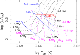
Figure 1: Position of V410 Tau (red) in the Hertzsprung-Russell diagram. The curves yielded by the Siess models (with solar metallicity and overshooting) are represented in black and those yielded by the Baraffe models are represented in magenta. In both cases, evolution tracks are displayed in dashed lines, except the Siess 1.4 ${\rm M}_{\odot}$ track, the one we chose to model the evolution of V410 Tau, which is shown as a full line. Isochrones are displayed in dotted lines. The thresholds where the radiative core starts developping ("Full convection") and where it reaches 25% of the stellar radius, according to the Siess models, are marked in blue.

Table 1: Physical parameters of wTTS V410 Tau. From top to bottom: distance from Earth, effective temperature, rotation period, luminosity, minimum stellar radius, stellar radius, line-of-sight-projected equatorial velocity, inclination, mass and age.

Parameter	Value	Reference
$d$	129.0 $\pm$ 0.5 pc	Galli et al. (2018)
$T_{\rm eff}$	4500 $\pm$ 100 K
$P_{\rm rot}$	1.87197 $\pm$ 0.00010 d	Stelzer et al. (2003)
$\log(\hbox{$L_{\star}$}/\hbox{${\rm L}_{\odot}$})$	0.63 $\pm$ 0.13
$R_{\star}$$\sin i$	2.708 $\pm$ 0.007 ${\rm R}_{\odot}$
$R_{\star}$	3.4 $\pm$ 0.5 ${\rm R}_{\odot}$
$v\sin i$	73.2 $\pm$ 0.2 km s-1	ZDI (Section 4)
$i$	50 $\pm$ 10°	ZDI (Section 4)
$M_{\star}$	1.42 $\pm$ 0.15 ${\rm M}_{\odot}$
Age	0.84 $\pm$ 0.20 Myr

4 Stellar tomography

To map the surface brightness and magnetic topology of V410 Tau, we use the tomographic technique ZDI (Brown et al., 1991; Donati & Brown, 1997), which inverts simultaneous time-series of Stokes $I$ and Stokes $V$ LSD profiles into brightness and magnetic field surface maps. At each observation date, Stokes $I$ and Stokes $V$ profiles are synthesized from model maps by integrating the spectral contribution of each map cell over the visible half of the stellar surface, Doppler-shifted according to the local RV (i.e. line-of-sight-projected velocity) and weighted according to the local brightness, cell sky-projected area and limb darkening. The main modifier of local RV at the surface of the star is, in ZDI, the assumed rotation profile at the stellar surface, e.g. the solid-body rotation of the star or a square-cosine-type latitudinal differential rotation. Local Stokes $I$ and Stokes $V$ line profiles are computed from the Unno-Rachkovsky analytical solution to the polarized radiative transfer equations in a Milne-Eddington model atmosphere (this is where the local magnetic field and the Zeeman effect intervene, see Landi degl’Innocenti & Landolfi, 2004). To fit the LSD profiles of V410 Tau in this study, we chose a spectral line of mean wavelength, Doppler width, Landé factor and equivalent width of respective values 640 nm, 1.8 km s^-1, 1.2 and 3.8 km s^-1.

ZDI uses a conjugate gradient algorithm to iteratively reconstruct maps whose synthetic profiles can fit the LSD profiles down to a user-provided reduced chi-square ($\chi^{2}_{\rm r}$) level. To lift degeneracy among the multiple solutions compatible with the data at the given reduced chi square, ZDI looks for the maximal-entropy solution, considering that the minimized information from the resulting maps is the most reliable. While the brightness value can vary freely from cell to cell, the surface magnetic field is modelled as a combination of poloidal and toroidal fields, both represented as weighted sums of spherical harmonics and projected onto the spherical coordinate space (Donati et al., 2006, for the equations). In this study, the magnetic field was fitted with spherical harmonics of orders $l=1$ to $l=15$.

Because ZDI does not reconstruct intrinsic temporal variability except for differential rotation, there is a limit to the duration a fittable data set can span. At the same time, ZDI needs a good phase coverage from the data to build a complete map. For those reasons, ZDI was not applied to runs 2008 Oct and 2013 Nov; moreover, we reconstructed a different set of brightness and magnetic images for each of the runs on which ZDI was applied.

Using ZDI on our data yielded values for $v\sin i$ and $i$ of ${73.2\pm 0.5}$ km s^-1 and ${50\pm 10}$° respectively. We also adjusted the systemic RV of V410 Tau with ZDI, and noticed a drift in the optimal value with time (see Table 2).

Table 2: Characteristics of the ZDI models for V410 Tau at each observation epoch. Column 1: observation epoch. Column 2: number of spectropolarimetric observations used for ZDI. Column 3: contribution of cool ("spots") and hot ("plages") areas on the brightness map. Column 4: average magnetic strength, defined as the square root of the average squared magnetic field over the surface of the star. Columns 5 to 7: normalized contribution of the poloidal field, part of the poloidal field that is dipolar and part of the poloidal field that is symmetric. Columns 8-9: part of the toroidal field that is dipolar and part of the toroidal field that is symmetric. Column 10: dipole characteristics: field strength, tilt with respect to the rotation axis and phase of the pole. Column 11: systemic RV of the star as measured with ZDI, the error bar on those values is 0.20 km s^-1. Error bars on the magnetic field ratios are typically of 0.1.

Date	Nobs	Spot+plage	B	$r_{\rm pol}$	$r_{\rm dip/pol}$	$r_{\rm sym/pol}$	$r_{\rm dip/tor}$	$r_{\rm sym/tor}$	Dipole strength (G),	RVbulk
		coverage (%)	(G)						tilt & phase	(km s-1)
2008 Dec	6	5.8+4.4	486	0.32	0.13	0.37	0.89	0.96	129, 23° & 0.71	16.30
2009 Jan	48	9.6+7.1	556	0.55	0.26	0.09	0.54	0.79	165, 54° & 0.54	16.30
2011 Jan	20	8.1+6.6	560	0.40	0.24	0.23	0.72	0.85	239, 44° & 0.62	16.40
2013 Dec	25	11.0+7.5	568	0.49	0.23	0.34	0.66	0.81	254, 18° & 0.56	16.50
2015 Dec	21	8.9+6.7	600	0.68	0.37	0.45	0.62	0.78	458, 30° & 0.54	16.65
2016 Jan	9	7.9+6.5	480	0.77	0.38	0.30	0.68	0.87	400, 44° & 0.51	16.65

4.1 Brightness and magnetic imaging

Time-series of Stokes $I$ and Stokes $V$ LSD profiles are shown in Figure 2, both before and after removal of lunar pollution, as well as synthetic profiles generated from the reconstructed ZDI maps. The corresponding maps are shown in Figure 3, with brightness maps in the first column and radial, meridional and azimuthal components of the surface magnetic field in the second to fourth columns. Properties of these reconstructed maps are listed in Table 2. Since the 2008 Dec data set has a phase coverage of only half the star, the derived parameters characterizing the global field topology at this epoch are no more than weakly meaningful and were not used for the following analysis and discussion. Our data have been fitted down to ${\hbox{$\chi^{2}_{\rm r}$}=1}$ with a feature coverage between 15 % and 18 % depending on the epochs, and a large-scale field strength of 0.5-0.6 kG. Since ZDI is only sensitive to mid- to large-scale surface features, and returns the maximum-entropy solution, this amount of spot coverage is not discrepant with the assumption made in Section 3; it further suggests that  30% of the star is more or less evenly covered with small-scale dark features.

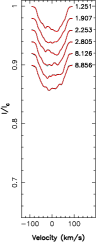
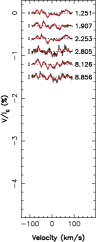
(a) 2008 Dec

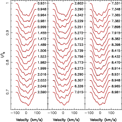
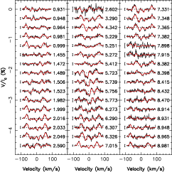
(b) 2009 Jan

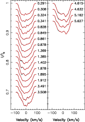
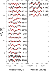
(c) 2011 Jan

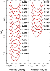
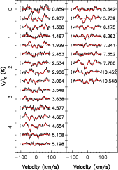
(d) 2013 Dec

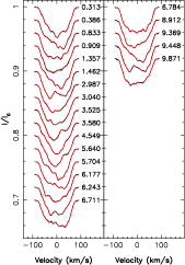
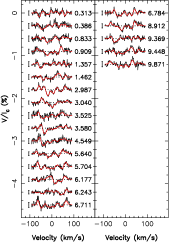
(e) 2015 Dec

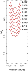
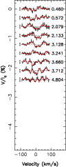
(f) 2016 Jan

Figure 2: LSD profiles for observation epochs 2008 Dec (a), 2009 Jan (b), 2011 Jan (c), 2013 Dec (d), 2015 Dec (e) and 2016 Jan (f). On the right of each profile is written the corresponding rotation cycle as indicated in Table 7. The cyan, black and red lines represent respectively the profiles before removal of Moon pollution, after removal of Moon pollution and the fit obtained with Zeeman Doppler Imaging. For each epoch, Stokes $I$ profiles are on the left and Stokes $V$ profiles on the right. 3$\sigma$-error bars are displayed beside each Stokes $V$ profile.

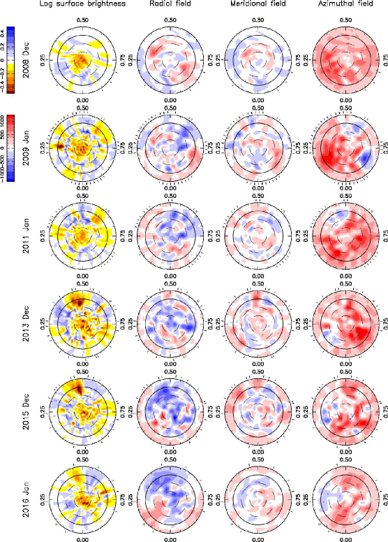
Figure 3: ZDI maps of the logarithmic relative surface brightness (first column), and the radial, meridional and azimuthal magnetic field (second to fourth columns) of V410 Tau, reconstructed from data collected in 2008 Dec, 2009 Jan, 2011 Jan, 2013 Dec, 2015 Dec and 2016 Jan (top to bottom rows). Each map is shown as a flattened polar view, with the equator being represented as a full line, and 60°, 30°, and -30° latitude parallels as dashed lines, and ticks around the star mark the spectropolarimetric observations. For the brightness maps, cool spots are colored in brown and bright plages in blue. For the magnetic maps, red represents outwards and anti-clockwise field on the radial and azimuthal field maps respectively, and the direction of the visible pole on the meridional field maps.

Brightness maps display a complex structure with many relatively small-scale features, and a high contrast. At all epochs, a large concentration of dark spots is observed at the pole. In 2009 Jan, 2013 Dec and 2015 Dec, the brightness map exhibits a strong equatorial spot, respectively at phases 0.27, 0.48 and 0.48. The presence of a strong polar spot is consistent with the maps published in Skelly et al. (2010), Rice et al. (2011) and Carroll et al. (2012) for data set 2009 Jan. At that particular epoch, the equatorial spot at phase 0.27, and another equatorial spot at phase 0.60, are also visible in both Skelly et al. (2010) and Rice et al. (2011) (figure 8), albeit less contrasted compared to other features than they are on our map. A remnant of the 2015 Dec equatorial spot is observed on the 2016 Jan map, where its intensity seems to have decreased, but this has to be taken with caution since ZDI maps are somewhat dependent on phase coverage. Dark spots and bright plages contribute to the feature coverage at about 9 % / 7 % respectively.

Photometry curves from the ZDI brightness maps were synthesized and a comparison to contemporary CrAO data, and WASP data in the case of 2011 Jan, is shown in Figure 4. Despite a slightly underestimated amplitude at phase 0.60 in 2008b-2009a, at phase 0.20 in 2011a, at phase 0.20 in 2013b and at phases 0.20 and 0.80 in 2015b-2016a, ZDI manages to retrieve the measured photometric variations of V410 Tau rather satisfyingly. We notice a small temporal evolution of the light curve in the WASP data during season 2010b-2011a, where the regions around phases 0.20 and 0.70 globally darken by 0.02-0.03 mag ($\simeq 4\sigma$) over the 4 months that the data set spans.

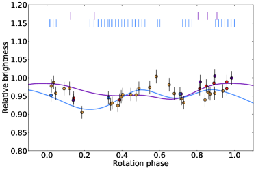
(a) 08b & 09a

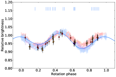
(b) 10b+11a

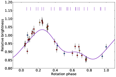
(c) 13b+14a

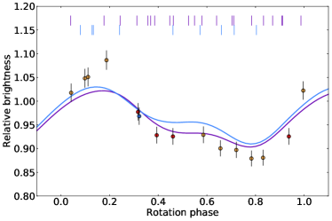
(d) 15b & 16a

Figure 4: Phase-folded photometry data (dots with 1$\sigma$ error bars) and ZDI models (lines) for observation epochs 08b & 09a (a), 10b+11a (b), 13b+14a (c) and 15b & 16a (d). In the case of 08b & 09a and 15b & 16a, two ZDI curves are plotted for the two ZDI maps reconstructed within each epoch. Orange, red, purple and blue colors each indicate a quarter of the total time span of the observations (photometric and spectropolarimetric together), in chronological order. Spectropolarimetric observations are marked by ticks above the light curves. In Figure b, WASP data were added as desaturated crosses, with the size of the cross branches indicating their 1$\sigma$ error bars.

The magnetic field maps also show a high complexity, with a poloidal component that has a weak dipolar contribution and that is rather non-axisymmetric, and a toroidal component contributing to $\sim$50% of the overall magnetic energy in 2009, 2011 and 2013, and decreasing towards ${\simeq 30}$ % in 2015-2016, that is both strongly dipolar and highly axisymmetric. The dipole pole is tilted at various angles depending on the epoch, with a tilt as high as 54° in 2009 Jan, down to 18° in 2013 Dec. The phase of the pole is always around 0.50-0.60, and the intensity of the poloidal dipole increases over time, from 165 G in 2009 Jan to ${\simeq 400}$ G in 2015-2016. We note that the maximum emission of H${\alpha}$ corresponds to the phase at which the dipole is tilted (Fig. 25). For visualisation purposes, 3-dimensional potential fields were extrapolated from the radial components of the magnetic maps, and displayed in Figure 5, with phase 0.50 facing the reader.

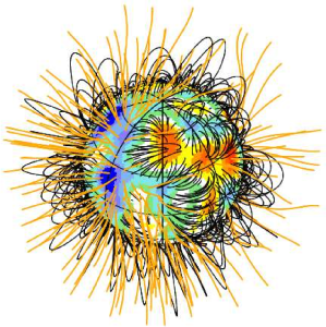
(a) 2009 Jan

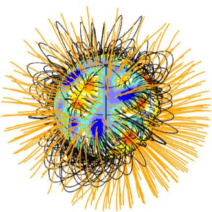
(b) 2011 Jan

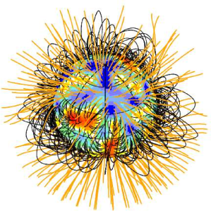
(c) 2013 Dec

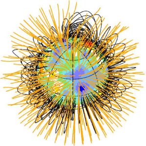
(d) 2015 Dec

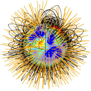
(e) 2016 Jan

Figure 5: Potential field extrapolations of the ZDI-reconstructed surface radial field, as seen by an Earth-based observer, for observation epochs 2009 Jan (a), 2011 Jan (b), 2013 Dec (c), 2015 Dec (d) and 2016 Jan (e) at phase 0.50. Open/closed field lines are shown in orange/black respectively, and colours on the stellar surface depict the local value of the radial field (in G, as shown in the left-hand panels of Fig. 3). The source surface at which field lines open is set to 2.1 $R_{\star}$, corresponding to the corotation radius and beyond which field lines are expected to quickly open under centrifugal forces given the high rotation rate of V410 Tau.

We do not observe a particular correlation between our brightness and our magnetic maps, meaning the areas with strong magnetic field are not necessarily crowded with dark spots, according to the ZDI reconstruction.

4.2 Differential rotation

Without differential rotation, ZDI cannot fit an extended data set, such as 2008 Dec + 2009 Jan, 2013 Nov + 2013 Dec or 2015 Dec + 2016 Jan (shortened in this subsection to 08b+09a, 13b and 15b+16a respectively), down to $\chi^{2}_{\rm r}$=1, it only manages to reach values of 1.66, 1.20 and 2.64 respectively. This implies that some level of variability exists and impacts the data on time scales of a few months, which could come from the presence of differential rotation at the surface of V410 Tau. We model differential rotation with the following law:

$$\Omega(\theta)=\hbox{$\Omega_{\rm eq}$}-(\cos\theta)^{2}\hbox{$d\Omega$}$$

where $\theta$ is the colatitude, $\Omega_{\rm eq}$ the equatorial rotation rate and $d\Omega$ the pole-to-equator rotation rate difference. We constrain $\Omega_{\rm eq}$ and $d\Omega$ by pre-setting the amount of information ZDI is allowed to reconstruct, and having ZDI minimize the $\chi^{2}_{\rm r}$ in these conditions.

We performed this analysis on the three afore-mentioned extended data sets, and on Stokes $I$ and Stokes $V$ time-series separately, reconstructing only brightness or only magnetic field respectively. From the resulting $\chi^{2}_{\rm r}$ maps over the {$\Omega_{\rm eq}$,$d\Omega$} space, one can plot the contours of the 1$\sigma$- (68.3%) and 3$\sigma$- (99.7%) areas of confidence for each observation epoch. Figure 6, which shows such contours, highlights clear minima surrounded by almost elliptic areas of confidence at each epoch, and shows that each 3$\sigma$-confidence area overlaps at least two other 3$\sigma$-confidence areas. Numerical results for each epoch are given in Table 3. We chose to use a unique set of parameters to reconstruct all images shown in Section 4: the weighted means of the six seasonal minima, ${\hbox{$\Omega_{\rm eq}$}=3.35957\pm 0.00006}$ rad d^-1 and ${\hbox{$d\Omega$}=0.0097\pm 0.0003}$ rad d^-1.

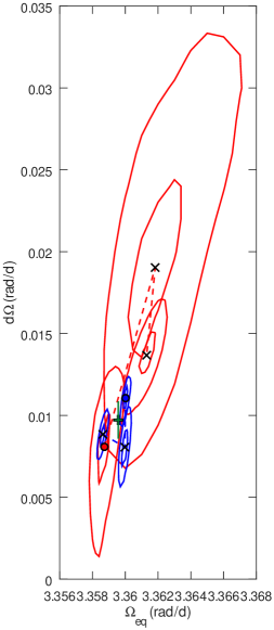
Figure 6: Evolution of the differential rotation of V410 Tau as measured from Stokes $I$ (blue) and Stokes $V$ (red) profiles. The points corresponding to observation epoch 2008b-2009a are marked with o symbols, then the dashed lines link the epochs in chronological order (2013b-2014a and 2015b-2016a are marked with x symbols). 68.3% and 99.7% contours of confidence are displayed for each observation epoch. The weighted average of the six measurements, chosen to produce the maps shown in Section 4, is represented as a black +, with overlayed error bars in green.

Following the method described in Donati et al. (2003), we computed, for each epoch, the colatitude at which the rotation rate is constant along the confidence ellipse major axis. This value corresponds to the colatitude where the barycenter of the brightness/magnetic features imposing a correlation between $\Omega_{\rm eq}$ and $d\Omega$ are located. For both Stokes $I$ and Stokes $V$, we note a slight increase with time of the cosine of this colatitude (Table 3), i.e. an increase in the barycentric latitude of the dominant features of ${5\pm 2}$° and ${15\pm 5}$° respectively.

Table 3: Summary of differential rotation parameters obtained for V410 Tau on each season. All rotation rates are given in mrad d^-1. Column 2 gives the total number of data points used in the imaging process, then columns 3 to 7 correspond to Stokes $I$ data while column 8 to 12 correspond to Stokes $V$ data. Columns 3 and 8 list the derived equatorial rotation rate $\Omega_{\rm eq}$, with its 68% (i.e. 1$\sigma$) confidence interval, columns 4 and 9 the difference in rotation rate $d\Omega$ between the equator and pole, with its 68% confidence interval, columns 5 and 10 give the reduced chi square of the ZDI model compared to the data, columns 6 and 11 give the inverse slope of the ellipsoid in the $\Omega_{\rm eq}$-$d\Omega$ plane (also equal to $\cos^{2}\,\theta_{s}$, where $\theta_{s}$ denotes the colatitude of the gravity centre of the spot distribution, see Donati et al. 2000), and columns 7 and 12 give the rotation rate $\Omega_{s}$ at colatitude $\theta_{s}$.

		|	Stokes $I$ data / brightness reconstruction					|	Stokes $V$ data / magnetic field reconstruction
Epoch	$n$	|	$\Omega_{\rm eq}$	$d\Omega$	$\chi^{2}_{\rm r}$	$\cos^{2}\,\theta_{s}$	$\Omega_{s}$	|	$\Omega_{\rm eq}$	$d\Omega$	$\chi^{2}_{\rm r}$	$\cos^{2}\,\theta_{s}$	$\Omega_{s}$
08b+09a	5562	|	3360.0 $\pm$ 0.1	11.1 $\pm$ 0.6	1.276	0.12 $\pm$ 0.03	3358.7 $\pm$ 0.4	|	3358.7 $\pm$ 0.3	8.1 $\pm$ 1.8	1.127	0.11 $\pm$ 0.03	3357.9 $\pm$ 0.5
13b	2781	|	3360.0 $\pm$ 0.1	8.1 $\pm$ 0.7	1.341	0.11 $\pm$ 0.03	3359.1 $\pm$ 0.3	|	3361.8 $\pm$ 1.3	19.0 $\pm$ 4.3	1.038	0.23 $\pm$ 0.03	3354.6 $\pm$ 2.1
15b+16a	3090	|	3358.6 $\pm$ 0.1	8.8 $\pm$ 0.5	2.583	0.18 $\pm$ 0.03	3357.0 $\pm$ 0.4	|	3361.3 $\pm$ 0.4	13.7 $\pm$ 1.0	1.046	0.32 $\pm$ 0.03	3352.7 $\pm$ 0.8

These models exclude solid-body rotation at a level of 3.6 to 22$\sigma$ depending on the epoch. We note that, even with differential rotation, ZDI cannot fit the data of 08b+09a and of 15b+16a down to $\chi^{2}_{\rm r}$=1, no matter the amount of information allowed. This indicates that surface features are also altered by a significant level of intrinsic variability within the 2-month span of our data set. This issue is further discussed in section 5.3.

5 Radial velocities

Radial velocity values were derived as the first-order moment of the continuum-subtracted Stokes $I$ LSD profiles, for all spectra except the 3 with low S/N and the 6 in which we identified flares (see Table 7). The raw RVs we obtain contain a contribution from the inhomogeneities on the photosphere, called activity jitter, which we aim to filter out in order to access the actual RV of the star, and look for a potential planet signature. The activity jitter is modelled with two different techniques, ZDI and Gaussian Process Regression. Raw RVs and jitter models are plotted in Figure 7 and listed in Table 7. For the 2015-2016 points, a new version of ZDI, with the logarithmic brightness of surface features allowed to lineary vary with time, was tested (section 5.3). The raw RVs present modulations whose amplitude vary between 4 and 8.5 km s^-1, with a global rms of 1.8 km s^-1. Like with the photometric data, the RV variations are the lowest in 2009 Jan and the strongest in 2013 Dec.

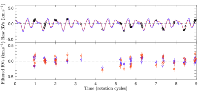
(a) 2009 Jan. Respective rms: 1.20, 0.13, 0.08 km s^-1

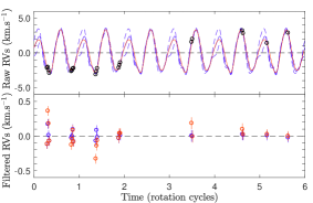
(b) 2011 Jan. Respective rms: 2.40, 0.14, 0.06 km s^-1

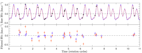
(c) 2013 Dec. Respective rms: 2.43, 0.22, 0.09 km s^-1

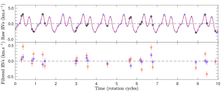
(d) 2015 Dec. Respective rms: 1.93, 0.22, 0.08 km s^-1

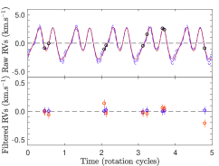
(e) 2016 Jan. Respective rms: 1.41, 0.09, 0.01 km s^-1

Figure 7: Raw and filtered RVs of V410 Tau for each observation epoch. On each figure, the top plot depicts the raw RVs (red dots), the ZDI reconstruction (red full line) and the GP fit (blue full line with 1-$\sigma$ area of confidence marked as blue dashed lines, see Section 5.1). The bottom plot depicts the RVs filtered from the ZDI-modelled activity (red dots) and the RVs filtered from the GP-modelled activity (blue dots). The subcaptions indicate the rms of the raw RVs, the ZDI-filtered RVs and the GPR-filtered RVs respectively. All rotational cycles are displayed as in Table 7.

5.1 Activity jitter

The first method consists in deriving the activity jitter from the ZDI models (see Fig. 2), computed as the first-order moment of the continuum-subtracted synthetic Stokes $I$ profiles. Indeed, when computing the raw RV from the observed Stokes $I$ LSD profiles, this activity jitter is added on top of the radial motion of the star as a whole. We model the activity jitter separately for epochs 2009 Jan, 2011 Jan, 2013 Dec, 2015 Dec and 2016 Jan (excluding 2008 Dec because of the poor phase coverage).

The second method uses Gaussian Process Regression (Haywood et al., 2014; Donati et al., 2017), a numerical method focusing on the statistical properties of the model. In short, GPR extrapolates a continuous curve described by a given covariance function from some given data points. To describe the activity jitter here, we use a pseudo-periodic covariance function:

$$K(t,t^{\prime})=\theta_{1}^{2}.\exp\left[-\frac{(t-t^{\prime})^{2}}{\theta_{3}^{2}}-\frac{\sin^{2}\left(\frac{\pi(t-t^{\prime})}{\theta_{2}}\right)}{\theta_{4}^{2}}\right]$$ (2)

where $t$ and $t^{\prime}$ are the dates of the two RV points between which the covariance is computed, $\theta_{1}$ is the amplitude of the GP, $\theta_{2}$ the recurrence time scale (expected to be close to $P_{\rm rot}$), $\theta_{3}$ the decay time scale (i.e., the typical spot lifetime in the present case) and $\theta_{4}$ a smoothing parameter (within [0, 1]) setting the amount of high frequency structures that we allow the fit to include. The modelling process therefore consists in optimizing the 4 parameters $\theta_{1}$, $\theta_{2}$, $\theta_{3}$ and $\theta_{4}$, called hyperparameters. To do so, we use a Markov Chain Monte-Carlo algorithm, and allocate to each point of the hyperparameter space a likelihood value, which takes into account both the quality of the fit and some penalizations on the hyperparameters (for example we penalize high amplitudes, low decay times and low smoothings). The priors are listed in Table 4. The phase plot of the MCMC is displayed in Figure 8 and the best fit is shown in Figure 7, together with the ZDI fits. We note that, contrary to ZDI, GPR, being capable of describing intrinsic variability in a consistent way, is able to fit our whole 8-year-long data set with one model. We obtain ${\theta_{1}=1.8^{+0.2}_{-0.2}}$ km s^-1, ${\theta_{2}=0.9991\pm 0.0002}$ $P_{\rm rot}$, ${\theta_{3}=86^{+24}_{-19}}$ $P_{\rm rot}$ and ${\theta_{4}=0.35\pm 0.03}$ $P_{\rm rot}$.

Table 4: Priors for our GP-MCMC run on our raw RVs. For the modified Jeffreys prior, the knee value is given, for the Gaussian prior we give the mean and standard deviation, and for the Jeffreys and the uniform priors we give the lower and upper boundaries.

Hyperparameter	Prior
$\theta_{1}$ (km s-1)	Modified Jeffreys ($\sigma_{\rm RV}$)
$\theta_{2}$ ($P_{\rm rot}$)	Gaussian (1.0000, 0.1000)
$\theta_{3}$ ($P_{\rm rot}$)	Jeffreys(0.1, 500.0)
$\theta_{4}$	Uniform (0, 1)

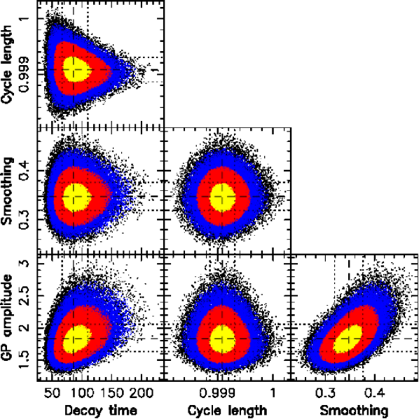
Figure 8: Phase plot of the MCMC-GPR run on the raw RVs, model without planet. The yellow, red and blue colors indicate respectively the 1$\sigma$-, 2$\sigma$- and 3$\sigma$-areas of confidence, and the optimal values for the hyperparameters are marked with black dashed lines, with 1$\sigma$-intervals marked with black dotted lines. GP amplitude ($\theta_{1}$): $1.8^{+0.2}_{-0.2}$ km s^-1, Cycle length ($\theta_{2}$): $0.9991\pm 0.0002$ $P_{\rm rot}$, Decay time ($\theta_{3}$): $86^{+24}_{-19}$ $P_{\rm rot}$, Smoothing ($\theta_{4}$): $0.35\pm 0.03$.

The rms of the filtered RVs for each epoch and each method are summarized in Table 5. The RV curve filtered from the ZDI model presents a global rms of 0.167 km s^-1, i.e. ${\sim 2<\sigma_{\rm RV}>}$ (see Table 7). The epoch where the filtering is most efficient is 2009 Jan, although the rms of the filtered RVs is only at 1.5${<\sigma_{\rm RV}>}$, and it goes up to 3${<\sigma_{\rm RV}>}$ in 2011 Jan and 2013 Dec. On the other hand, the GPR model filters the RV out down to 0.076 km s^-1 = 0.94${<\sigma_{\rm RV}>}$.

Table 5: Rms of RVs. All rms RVs are given in km s^-1.

Epoch	2009	2011	2013	2015	2016	All
Raw	1.200	2.392	2.429	1.932	1.411	1.8
ZDI filt.	0.131	0.141	0.215	0.222	0.094	0.167
GP filt.	0.084	0.064	0.087	0.075	0.009	0.076

5.2 Periodograms

Lomb-Scargle periodograms for both raw and filtered RVs, for both methods (Fig. 9 for each individual epoch, 10 for the whole data set), show that the stellar rotation period or its first harmonic are clearly present in 2009 Jan and 2011 Jan, but not well retrieved in 2013 Dec, 2015 Dec and 2016 Jan. However the periodogram for the whole ${\rm RV}_{\rm raw}$ data set presents neat peaks at $P_{\rm rot}$ and its first two harmonics. $P_{\rm rot}$ and its first harmonic are well filtered out by both modelling methods, and the second harmonic is well filtered out in the GP residuals. A weak signal remains at $P_{\rm rot}$/3 in the ZDI residuals but looking at a phase-folded plot does not reveal any particularly obvious tendency, leading us to suspect that it mostly reflects the contribution of a few stray points. No other period stands out with a false-alarm-probability lower than 5%, which allows us to conclude that no planet signature is found in this data set with our filtering methods.

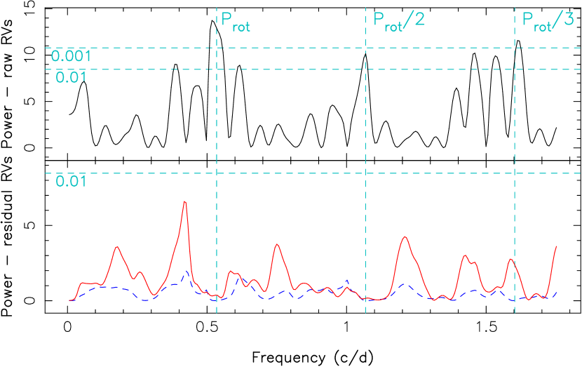
(a) 2009 Jan

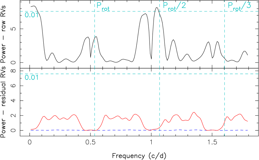
(b) 2011 Jan

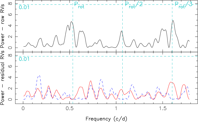
(c) 2013 Dec

Figure 9: Periodograms of the raw RVs (top), of the ZDI-filtered RVs (bottom, red full line) and of the GP-filtered RVs (bottom, blue dashed line), for observation epochs 2009 Jan (a), 2011 Jan (b), 2013 Dec (c), 2015 Dec (d) and 2016 Jan (e). False-alarm probability levels of 1% and 0.1% are represented as horizontal cyan dashed lines, and $P_{\rm rot}$ and its first two harmonics as vertical cyan dashed lines (continuing next page).

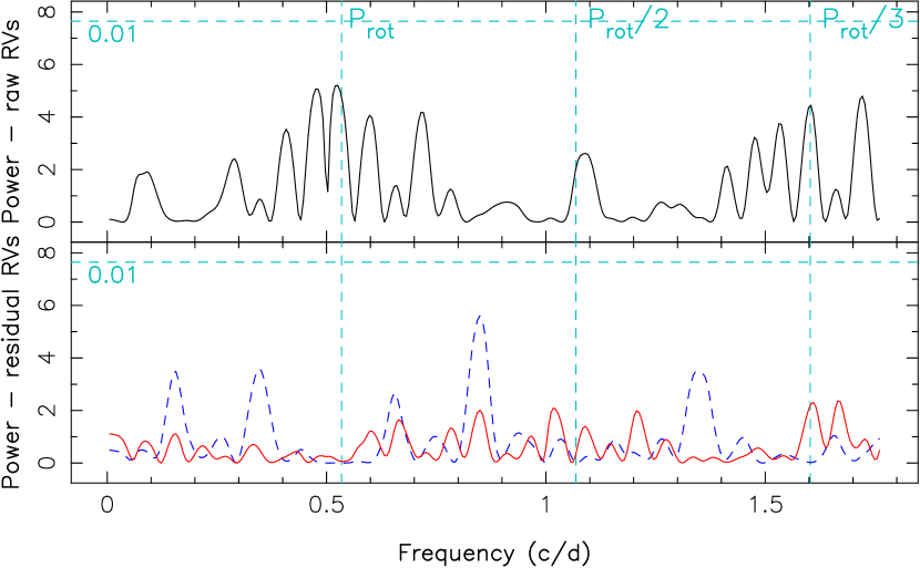
(d) 2015 Dec

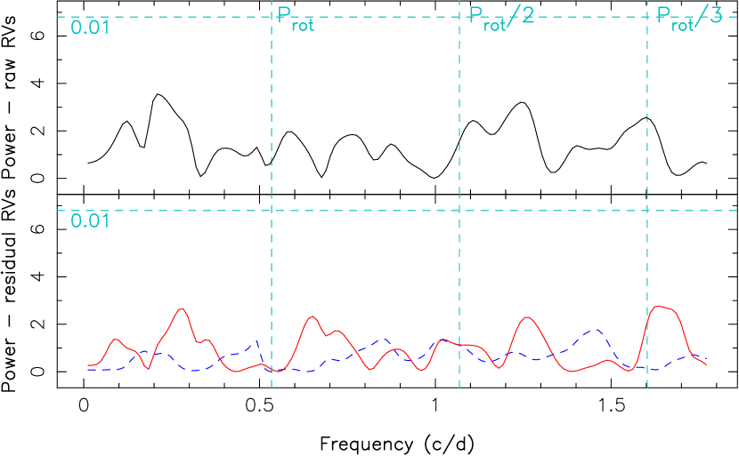
(e) 2016 Jan

Figure 9: (Continued from previous page).

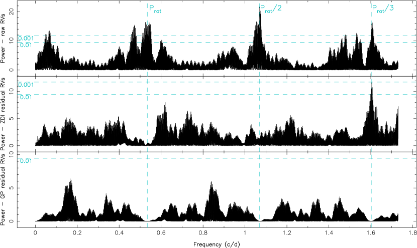
Figure 10: Periodograms of the raw RVs (top), of the RVs filtered from ZDI-modelled activity (middle) and of the RVs filtered from GP-modelled activity (bottom, blue dashed line), for observation epochs 2009 Jan (a), 2011 Jan (b), 2013 Dec (c), 2015 Dec (d) and 2016 Jan (e). Periodograms of the whole data set raw RVs (top), RVs filtered from ZDI-modelled activity (middle) and RVs filtered from GP-modelled activity (bottom). False-alarm probability levels of 1% and 0.1% are represented as horizontal cyan dashed lines, and $P_{\rm rot}$ and its first two harmonics as vertical cyan dashed lines.

5.3 New ZDI: with short-time intrinsic evolution

Seeing that the filtered RVs when using GPR have a rms twice lower than when using ZDI (Table 5), we try to improve our ZDI filtering process by implementing a new feature: instead of only having one brightness value in each cell, we give it a brightness value and an evolution parameter, so that ZDI brightness maps are allowed to evolve with time to better fit time-series of LSD profiles with variability. Thus we reconstruct two maps for the brightness: the brightness at time 0 and the map of the evolution parameter. We choose, for now, a simple model where the logarithmic relative brightness of each cell $k$ is allowed to evolve linearily with time:

$$\log Q_{k}(t)=\log Q_{k}(0)+m_{k}t,$$ (3)

where $Q_{k}(t)$ is the local surface brightness and $m_{k}$ is the evolution parameter. Applying this new method to the 2015-2016 extended data set, we manage to fit the whole data set down to a $\chi^{2}_{\rm r}$ of 1 where classical ZDI, even with differential rotation, could not reach lower than $\chi^{2}_{\rm r}$=2.5 (see Section 4.2). Maps associated to this reconstruction are shown in Fig. 11, and derived RVs are plotted in Fig. 12 and 13, to be compared with RVs derived from classical ZDI maps. The rms of the filtered RVs here, 0.194 km s^-1, does not decrease compared to when using classical ZDI, which means our model is still too simple and cannot fully account for the observed variability. However, Fig. 13 shows that global trends in the temporal evolution of the RV curve are well-reproduced by this new ZDI model, such as the jitter maximum moving from phase 0.37 to 0.32, or the local minimum at phase 0.54 in 2015 Dec moving to 0.50 in 2016 Jan.

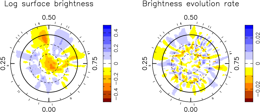
Figure 11: Brightness map and evolution rate reconstructed by ZDI on data set Dec 2015-Jan 2016. Pole-on view with the equator being represented as a full line, and 60°, 30°, and -30° latitude parallels as dashed lines. Cool spots are colored in brown and bright plages in blue, and ticks around the star mark the spectropolarimetric observations.

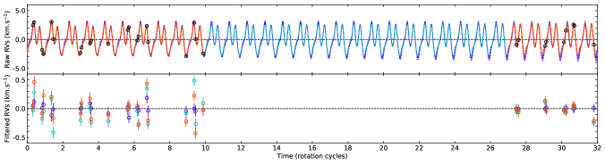
Figure 12: Comparison between the GP model, the new ZDI model and the classical ZDI models for V410 Tau RVs in season 2015b-2016a. Rotation cycles are offset to concur with Table 7. Top: raw RVs (black dots) with $1\sigma$-error bars, GP model (purple full line), new ZDI model (cyan full line) and classical ZDI models for both observation epochs 2015 Dec and 2016 Jan (red full lines). Bottom: RVs filtered from the GP model (purple dots), from the new ZDI model (cyan dots) or from the classical ZDI models (red dots). The rms of the filtered RVs with GP, new ZDI and classical ZDI are respectively 0.065, 0.194 and 0.193 km s^-1.

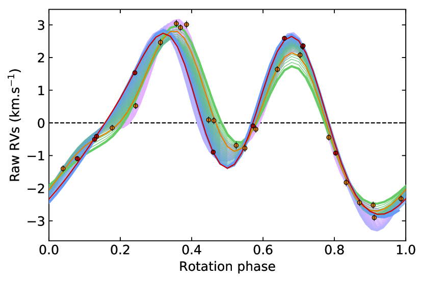
Figure 13: Raw RVs of V410 Tau in the 2015b-2016a season, between cycles 1349 and 1381 as referenced in Table 7, plotted against stellar rotation phase. The GPR and new ZDI models are represented by full lines colored in gradients, from earliest to latest cycle, respectively pink to purple and green to blue, while the classical ZDI models for 2015 Dec and 2016 Jan are plotted in orange and red respectively. Observations are plotted as dots with 1$\sigma$-error bars, orange for 2015 Dec and 2016 Jan.

6 Summary and discussion

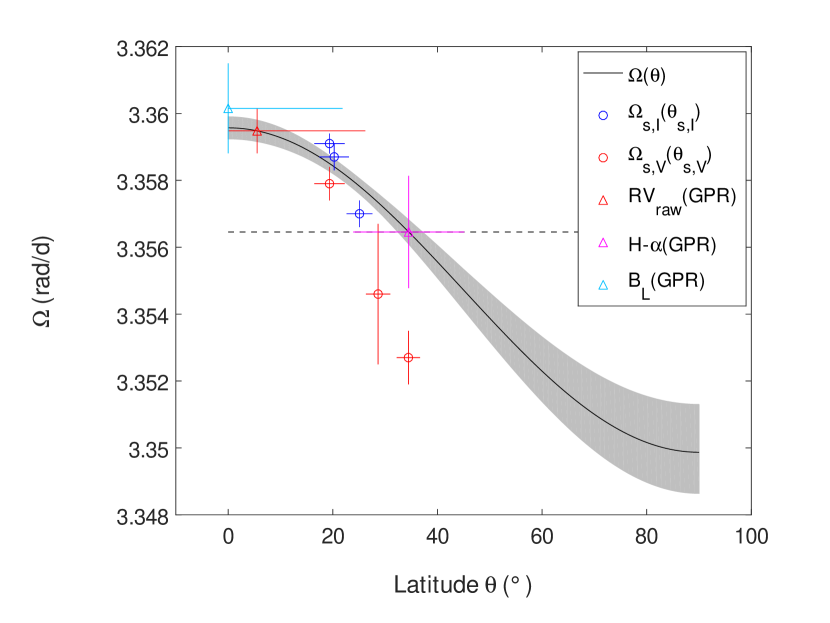
Figure 14: Differential rotation curve of V410 Tau (black full line) with 1$\sigma$ uncertainty in gray, with ${\hbox{$\Omega_{\rm eq}$}=3.35957\pm 0.00006}$ rad d^-1 and ${\hbox{$d\Omega$}=0.0097\pm 0.0003}$ rad d^-1. The stellar rotation rate chosen to phase our data is represented as a dashed horizontal line. The rotation rates derived from the RVs (red), from the H${\alpha}$ equivalent widths (magenta) and from the longitudinal field measurements (cyan) are positioned on the differential rotation curve as triangles with 1$\sigma$ error bars, thus yielding the barycentric latitude of the features determining the period. The dots represent couples ${\{90-\theta_{s},\Omega_{s}\}}$ derived in our epoch-wise differential rotation measurements, those coming from Stokes $I$ / Stokes $V$ data being plotted in blue / red respectively.

This paper reports the analysis of an extended spectropolarimetric data set on the $\sim$0.8 Myr wTTS V410 Tau, taken with the instruments ESPaDOnS at CFHT and NARVAL at TBL, spanning eight years and split between six observation epochs (2008b, 2009a, 2011a, 2013b, 2015b and 2016a), the last three of which were observed as part of the MaTYSSE observation programme. Contemporaneous photometric observations from the CrAO and from the WASP programme complemented the study. ESPaDOnS, NARVAL and CrAO observations are documented in Appendix A.

V410 Tau is composed of an inner close binary (V410 Tau A-B) around which orbits a third component (C Ghez et al., 1997), with V410 Tau A being much brighter than the other two in the optical domain, and thus the star that our data inform. The stellar parameters derived in this work are summed up in Table 1: at $\sim$0.8 Myr, V410 Tau is a ${1.42\pm 0.15}$ ${\rm M}_{\odot}$ and ${3.4\pm 0.5}$ ${\rm R}_{\odot}$ wTTS.

6.1 Activity and magnetic field of V410 Tau

Applying LSD then ZDI on our data set, we estimated the $v\sin i$ and inclination of V410 Tau at ${73.2\pm 0.5}$ km s^-1 and ${50\pm 10}$° respectively. Considering the well-determined rotation period of ${1.871970\pm 0.000010}$ (Stelzer et al., 2003) and the minimal observed visible magnitude of 10.52 (Grankin et al., 2008), this implies a relatively high level ($\sim$50%) of spot coverage. We reconstructed brightness and magnetic surface maps at each observation epoch, constrained the differential rotation and found a drift in the bulk radial velocity. Our ZDI brightness maps display a relatively highly spotted surface: the spot coverage reaches 6.5 to 11.5 percent depending on the epoch (not counting 2008 Dec where only half the star was imaged) and the plage coverage is found around 7 percent at all epochs. Since ZDI mostly recovers large non-axisymmetric features and misses small ones evenly distributed over the star, the spot and plage coverage is underestimated, which makes this result compatible with the spot coverage obtained from the aforementioned V magnitude measurements. We note that V410 Tau being heavily spotted makes it difficult to pinpoint its age. We fit a 2-temperature model (photosphere at 4500 K and fixed-temperature spots with a varying filling factor) into our B-V and V magnitude data, and found an optimal spot temperature of around 3750 K, which implies a contrast of $\sim$750 K between dark spots and the photosphere (see Fig. 24). This contrast is slightly lower than the one retrieved for the 2 Myr wTTS LkCa 4 in Gully-Santiago et al. (2017). V410 Tau always presents a high concentration of dark spots around the pole, and several big patches of dark spots on the equator.

V410 Tau has a relatively strong large-scale magnetic field, with an average surface intensity that is roughly constant over the years at ${550\pm 50}$ G. Its radial field reaches local values beyond -1 kG and +1 kG in several epochs. The brightness and magnetic surface maps both present some variability from epoch to epoch (Fig. 3, Table 2), which points to a dynamo-generated magnetic field rather than a fossil one. The magnetic energy is, at all epochs, equally distributed between the poloidal and toroidal components of the field, with the poloidal component being rather non-dipolar and non-axisymmetric, whereas the toroidal component is mostly dipolar and axisymmetric. The poloidal dipole, tilted towards a phase that stays within ${0.6\pm 0.1}$ during the whole survey, but at an angle varying between 20° and 55° depending on the epoch, sees its intensity increase almost monotonously from 165 G to 458 G over 8 years, and the dipolar contribution to the poloidal field also increases from $\sim$25% to $\sim$40% (see Table 2).

The toroidal component, which displays a constant orientation throughout our data set, is unusually strong compared to other fully convective rapidly-rotating stars (e.g. V830 Tau is 90 percent poloidal, see Donati et al., 2017). A similarly strong toroidal field was observed on one other MaTYSSE target, LkCa 4 (Donati et al., 2014). The origin of this strong toroidal field is still unclear: could it be maintained by an $\alpha^{2}$ dynamo, like in the simulations of low-Rossby fully convective stars by Yadav et al. (2015)? The remnants of a subsurfacic radial shear between internal layers accelerating due to contraction, and disc-braked outer layers? Or would the even earlier toroidal energy, from right after the collapse of the second Larson core (as found in the simulations of Vaytet et al., 2018), somehow not have entirely subsided yet? Would the early dissipation of the disc, a common factor between LkCa 4 and V410 Tau, have something to do with this?

At $\sim$0.8 Myr, V410 Tau is one of the youngest observed wTTSs (Kraus et al., 2012, Fig. 3). Assuming that, when the disc was present, V410 Tau was magnetically locked to it at a rotation period of $\sim$8 d with a cavity of $\sim$0.085 au (similarly to cTTSs BP Tau, AA Tau and GQ Lup, see Donati et al., 2008, 2010b, 2012, resp.), then V410 Tau should have had a radius of $\sim$7 ${\rm R}_{\odot}$ when the disc dissipated, to match the angular momentum that we measure today (Bouvier, 2007). According to the Siess models (Siess et al., 2000), this corresponds to an age of $\sim$0.2 Myr. With a radius of $\sim$7 ${\rm R}_{\odot}$, V410 Tau would have needed a magnetic dipole barely above $100$ G to maintain the assumed magnetospheric cavity, even with an accretion rate of ${\sim 10^{-8}}$ ${\rm M}_{\odot}$ ${\rm yr}^{-1}$ just before disc dissipation. That value is compatible with the 200-400 G dipole we measure on the $\sim$3.5 ${\rm R}_{\odot}$ star today. Kraus et al. 2012 (Fig. 1) shows a correlation between the presence of a close companion and the early depletion of the accretion disc, which indicates that V410 Tau B, observed at a projected separation of ${16.8\pm 1.4}$ au (Ghez et al., 1995), could have been responsible for the early depletion of the disc.

In our H${\alpha}$ dynamic spectra, we observe a conspicuous absorption feature in the second part of the 2009 Jan run around phase 0.95 (Fig. 25), that could be the signature of a prominence (see e.g. Collier Cameron & Woods, 1992). Fitting a sine curve in the absorption feature yields an amplitude of $\sim$2 $v\sin i$, corresponding to a prominence $\sim$2 $R_{\star}$ away from the center of V410 Tau, confirming that the prominence is located close to the corotation radius. Plotting the 3D potential field extrapolation of the reconstructed surface radial field for 2009 Jan, at phases 0.95, 0.20, 0.45 and 0.70, we observe the presence of closed field lines reaching $\sim$2 $R_{\star}$ at phase 0.95 (Fig. 15), which may be able to support the observed prominence. We also observe similar absorption features in 2009 Jan around phase 0.8 and in 2011 Jan around phase 0.35, but they are less well-covered by our observations. We however found corresponding field lines at the right phase for each (see Fig. 15 for 2009 Jan).

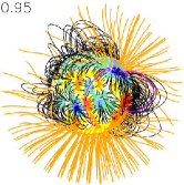
(a) Phase 0.95

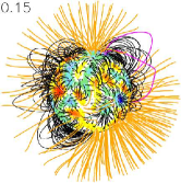
(b) Phase 0.15

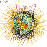
(c) Phase 0.35

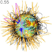
(d) Phase 0.55

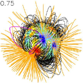
(e) Phase 0.75

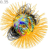
(f) Phase 0.35

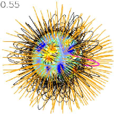
(g) Phase 0.55

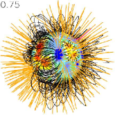
(h) Phase 0.75

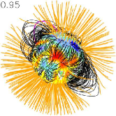
(i) Phase 0.95

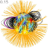
(j) Phase 0.15

Figure 15: Potential field extrapolations of the ZDI-reconstructed surface radial field, as seen by an Earth-based observer, for observation epochs 2009 Jan (top) and 2011 Jan (bottom) at different phases. Open/closed field lines are shown in orange/black respectively, and colours at the stellar surface depict the local value of the radial field (in G, as shown in the left-hand panels of Fig. 3). The source surface at which field lines open is set to 2.18 $R_{\star}$. The field lines that would carry the potential observed prominences (phase 0.95 and 0.8 in 2009, phase 0.35 in 2011) are colored in magenta. Animated versions with the star rotating are available at http://userpages.irap.omp.eu/~lyu/jan09a.gif and http://userpages.irap.omp.eu/~lyu/jan11n.gif.

We also constrained the differential rotation of V410 Tau with ZDI: we obtained six values for the equatorial rotation rate $\Omega_{\rm eq}$ and for the pole-to-equator rotation rate difference $d\Omega$, by using separately our Stokes $I$ and Stokes $V$ LSD profiles from each of the three data sets 2008b+2009a, 2013b and 2015b+2016a. Overall mean values are $\Omega_{\rm eq}$=${3.35957\pm 0.00022}$ rad d^-1 and $d\Omega$=${0.0097\pm 0.0011}$ rad d^-1. The differential rotation of V410 Tau is thus relatively weak, with a pole-to-equator rotation rate difference 5.6 times smaller than that of the Sun, and a lap time of ${648\pm 73}$ d. Compared to other wTTSs previously analyzed within the MaTYSSE programme, the differential rotation of V410 Tau is similar to that of V830 Tau (Donati et al., 2017) but much smaller than that of TAP 26, which is almost of solar level, consistent with the fact that TAP 26 is no longer fully convective and has developped a radiative core (of size 0.6 $R_{\star}$, Yu et al., 2017).

6.2 Mid-term variability of V410 Tau

Even with differential rotation, it is impossible for our current version of ZDI to model data sets spanning a few months down to noise level, which shows that the surface of V410 Tau undergoes significant instrinsic variability, corroborating the hypothesis of a dynamo-generated field. The variations of the photosphere and of the surface magnetic field over the years might be the manifestation of a magnetic cycle, whose existence has been suggested by previous studies (Stelzer et al., 2003; Hambálek et al., 2019). No clear change in $d\Omega$ is observed while the dipole grows in intensity (Table 3), which could indicate a time lag in the dynamo interaction between the magnetic field and the rotation profile.

The bulk RV of V410 Tau exhibits a drift throughout our 8-year campaign, from $16.30\pm 0.05$ km s^-1 in 2008b-2009a to $16.65\pm 0.05$ km s^-1 in 2015b-2016a. One explanation could be a variation in the suppression of convective blueshift in regions of strong magnetic field (Haywood et al., 2016; Meunier et al., 2010), which could further support a secular evolution of the magnetic topology. It could also be a manifestation of the binary motion of V410 Tau A-B. The central binary of V410 Tau was observed twice, with a sky-projected separation of $16.8\pm 1.4$ au in 1991 Oct and $9.5\pm 0.3$ au in 1994 Oct ($0.13\pm 0.01$ arcsec and $0.074\pm 0.002$ arcsec resp. in Ghez et al., 1995), and a mass ratio of $0.20\pm 0.10$ (Kraus et al., 2011). Assuming a mass ratio of 0.2 and an edge-on circular orbit, we find that an orbit of the primary star of radius 6.0 au, i.e. binary separation 36.0 au and period 166 a, fits our bulk RVs and the sky-projected separations at a level of $2\sigma$ (see Fig. 16). No binary motion was detected in the 2013 to 2017 astrometry measurements of Galli et al. (2018), which is consistent with our model where the sky-projected velocity varies by only 0.13 ${{\rm mas}\,a^{-1}}$ over these 3.5 years (roughly a 50th of the orbital period). More measurements would enable to estimate the eccentricity and potentially fit the sky-projected separations to a better level, as well as to decide whether the binary motion can explain the RV drift observed in this study.

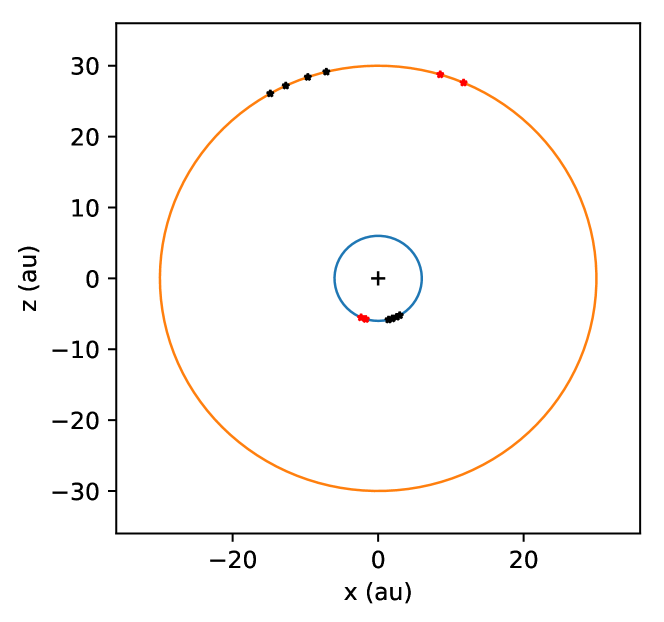
Figure 16: Circular model for the binary motion of V410 Tau A and V410 Tau B: edge-on orbit, separation 36.0 au, period 166 a and systemic radial velocity 16.06 km s^-1. Top: top-view of the model orbit, with the z-axis parallel to the line-of-sight, where the positions of V410 Tau A and B according to the model are marked by red and black stars at the times of the separation measurements and of our spectropolarimetric seasons (2008b-2009a, 2011a, 2013b and 2015b-2016a) respectively. Middle: RV_bulk of V410 Tau A with time, as measured by us in black dots with $1\sigma$ error bars and as derived from the model orbit in blue. The predicted RV_bulk at the times of the separation measurements are represented by red stars. Bottom: Sky-projected binary separation as a function of time, as measured by Ghez et al. 1995 in red dots with $1\sigma$ error bars, and as derived from the model orbit in blue. The predicted sky-projected separations at the dates of our observing seasons are marked in black stars.

The rotation period derived from our V magnitude measurements, in each observing season, also displays long-term variations. Placing the periods found from the photometric data on a period-latitude diagram representing the modeled differential rotation (Fig. 22), we observe that the latitudes corresponding to the successive periods tend to increase from 0 in 2008 to $\sim$50° in 2016. We note that this trend is observed with both the periods derived from sine fits to the photometric data and those derived from GPR (see B). This implies that the largest features, ie those with the biggest impact on the photometric curve, underwent a poleward migration, reminiscent of the Solar butterfly diagram (albeit reversed). This would suggest that the dynamo wave, if cyclic, has a period of at least 8 a and likely much longer (16 a if our data covers only one half of a full cycle). Previous studies using different data have suggested the existence of an activity cycle on V410 Tau, with periods of 5.4 a and 15 a respectively (Stelzer et al., 2003; Hambálek et al., 2019). We further note that our differential rotation measurements confirm that the barycenter of surface features migrates to higher latitudes over time (see Fig 6).

Applying GPR with MCMC parameter exploration to our H${\alpha}$ equivalent widths and longitudinal magnitude field measurements ($B_{\rm\ell}$, first-order moment of the Stokes $V$ LSD profiles, Donati & Brown, 1997), we also found rotation periods from which we derive mean barycentric latitudes of features constraining the modeling of each quantity (see Fig. 14). The period found from H${\alpha}$ is equal within error bars to the one derived in Stelzer et al. 2003 from photometry, whereas the period found from $B_{\rm\ell}$ seems tied to equatorial features. It is worth mentioning that we also find long decay times for these two activity proxies: ${589^{+774}_{-335}}$ d and ${604^{+553}_{-289}}$ d respectively, which suggests, with the caution needed with such high error bars, that the H${\alpha}$ and $B_{\rm\ell}$ modulations are particularly sensitive to large, long-lasting features. The phase plots are displayed in Appendix C.

Table 6: Various evolution time scales.

Quantity	Time scale (d)
RV decay time	$160^{+45}_{-35}$
V mag decay time	$314^{+31}_{-29}$
H${\alpha}$ decay time	$589^{+774}_{-335}$
$B_{\rm\ell}$ decay time	$604^{+553}_{-289}$
Differential rotation lap time	$648\pm 73$

6.3 Radial velocity modulations

We modeled the activity RV jitter from line profiles synthetized from our ZDI maps, and filtered it out from the RV curve of V410 Tau. From a rms of 1.802 km s^-1 in the raw RVs, we get residuals with a rms of 0.167 km s^-1. We also applied GPR to our raw RVs and found a jitter of periodicity ${1.87029\pm 0.00037}$ d and decay time ${160^{+45}_{-35}}$ d, with residuals of rms 0.076 km s^-1. The period derived from the GPR on our raw RVs is shorter than the period we used to phase our data, and corresponds to a latitude of 5.5°. This period is much closer to the period derived with GPR from $B_{\rm\ell}$ than to the period derived from H${\alpha}$, showing that in this case, $B_{\rm\ell}$ is a better activity proxy than H${\alpha}$ (for a more systematic study of the correlation of $B_{\rm\ell}$ with stellar activity, see Hébrard et al., 2016). The decay time associated to RVs is much shorter than the differential rotation lap time and the decay times of the V magnitude, H${\alpha}$ and $B_{\rm\ell}$ (see Table 6), which suggests that RVs are more sensitive to small-scale short-lived features while the photometry, H${\alpha}$ and $B_{\rm\ell}$ are more sensitive to large-scale long-lasting features.

Through both processes, the residual RVs present no significant periodicity which would betray the presence of a potential planet. To estimate the planet mass detection threshold, GPR-MCMC was run on simulated data sets, composed of a base activity jitter (our GP model from Section 5), and a circular planet signature, plus a white noise of level 0.081 km s^-1. Various planet separations and masses were tested, and for each case, GPR-MCMC was run several times with different randomization seeds, to mitigate statistical bias. For every randomization seed, GPR-MCMC was run with a model including a planet and a model including no planet, and the difference of logarithmic marginal likelihood between them (hereafter $\Delta\mathcal{L}$) was computed. Finally, the detection threshold was set at $\Delta\mathcal{L}=10$ and the minimum detectable mass at each separation was interpolated from the mass/$\Delta\mathcal{L}$ curve. Fig. 17 shows the planet mass detection threshold as a function of planet-star separation: we thus obtained a detectability threshold of $\sim$1 ${\rm M}_{\rm Jup}$ for ${a<0.09}$ au and $\sim$4.6 ${\rm M}_{\rm Jup}$ for ${a=0.15}$ au. The figure also shows the parameters of V830 Tau b and TAP 26 b, showing that we would likely have detected a planet like TAP 26 b but not one like V830 Tau b. Planets beyond $a=0.15$ au are difficult to detect due to the temporal coverage of our data, that never exceeds 19 d at any given epoch. The early depletion of the disc may have prevented the formation and/or the migration of giant exoplanets. Kraus et al. 2016 outlines a correlation between the presence of a close companion and a lack of planets, in a sample of binary stars with mass ratios $q>0.4$, which could support the hypothesis that V410 Tau B, although having a slightly lower mass ratio ($q=0.2\pm 0.1$, Kraus et al., 2011), played a role in the early disc dissipation, which in turn prevented the formation of a hot Jupiter.

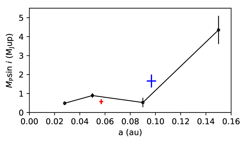
Figure 17: Detectability threshold in terms of $M\sin i$ for planets at various $a$, with the RV filtering technique involving GPR. V830 Tau b is plotted in red (parameters from Donati et al., 2017) and TAP 26 b in blue (parameters from Yu et al., 2017).

In terms of methodology, GPR fits the data down to a significantly lower $\chi^{2}_{\rm r}$ than ZDI because it is capable of accounting for most of the mid-term variability, contrarily to ZDI, which for now only integrates differential rotation and a simplistic description of intrinsic variability. Small strutures evolve on time scales of $\sim$few weeks, so we need to be able to model their temporal evolution in a more elaborate way to be able to match the capability of GPR to fit time-variable RV curves. Self-consistent methods that combine the physical faithfulness of ZDI and the flexibility of GPR will be developped in the near future and applied to more MaTYSSE data, as well as to data from the SPIRou (Spectropolarimetre InfraRouge) Legacy Survey (SLS). Finally, observing V410 Tau and other wTTSs with SPIRou will yield spectra in the near infrared, where we expect a smaller jitter than in the optical bandwidth, and will offer an opportunity to benchmark our activity jitter filtering technique performances.

¹ Univ. de Toulouse, CNRS, IRAP, 14 avenue Edouard Belin, 31400 Toulouse, France
² Crimean Astrophysical Observatory, Nauchny, Crimea 298409
³ SUPA, School of Physics & Astronomy, Univ. of St Andrews, St Andrews, Scotland KY16 9SS, UK
⁴ CFHT Corporation, 65-1238 Mamalahoa Hwy, Kamuela, Hawaii 96743, USA
⁵ ESO, Karl-Schwarzschild-Str 2, D-85748 Garching, Germany

Appendix A Observations

This appendix informs all the observations, both spectropolarimetric (Table 7) and photometric (Table 8), that we used in this study, excluding the WASP data. The spectropolarimetric data are spread over 8 runs (2008 Oct, 2008 Dec, 2009 Jan, 2011 Jan, 2013 Nov, 2013 Dec, 2015 Dec and 2016 Jan) and the photometric data are spread over 9 seasons: 08b+09a (short for 2008b + 2009a; all the other seasons follow the same naming convention), 09b+10a, 10b, 11b+12a, 12b+13a, 13b+14a, 14b, 15b+16a and 16b+17a.

The instruments with which the spectropolarimetric data was taken, ESPaDOnS and NARVAL, are twin spectropolarimeters and cover a 370 to 1000 nm wavelength domain, with respective resolving powers of 65 000 (i.e. resolved velocity element of 4.6 km s^-1) and 60 000 (resolved velocity element of 5.0 km s^-1). Each polarization exposure sequence consists of four subexposures of 600 s each, taken in different polarimeter configurations to allow the removal of all spurious polarization signatures at first order (Donati et al., 1997), except three observations comprised of only two subexposures of 600 s (2008 Dec 05 at phase 0.827, 2009 Jan 05 at phase 0.602, and 2013 Nov 07 at phase 0.541), and three observations comprised of four subexposures of 800 s (2009 Jan 10 at phases 0.229, 0.251 and 0.272).

Table 7: Information on the V410 Tau spectropolarimetric data. The first three columns contain the time at which the observations were taken: Coordinated Universal Time in the 1st column, Barycentric Julian Date in the 2nd and corresponding rotational cycle of V410 Tau, $c$, in the 3rd, as is defined in equation 1. The 4th column indicates the instrument used for the observation (E: ESPaDOnS, N: NARVAL) and column 5 the spectrum S/N. Column 6 indicates rejected spectra or the presence of moon pollution (^a: not used in ZDI, ^b: not used in GPR, ^c: not used for period retrieval from H${\alpha}$ EW). Columns 7 and 8 contain the S/N in the Stokes $I$ and Stokes $V$ LSD profiles respectively. Columns 9 to 12 show the raw RVs, the RVs filtered with ZDI, the RVs filtered with GPR and the 1$\sigma$ RV error bar respectively, column 13 lists the equivalent width of the H${\alpha}$ line (with a typical error bar of 10 km s^-1) and column 14 informs the longitudinal projection of the magnetic field integrated over the visible surface (with a typical error bar of 50 G).

UTC	BJD	Cycle	Instr.	S/N	Comment	S/NI	S/NV	RVraw	RVfilt/ZDI	RVfilt/GP	$\sigma_{\rm RV}$	EW${}_{\hbox{H${\alpha}$}}$	Blong
2008 Oct	2454700+	-42+						(km s-1)	(km s-1)	(km s-1)	(km s-1)	(km s-1)	(G)
15 11:42:34	54.992	0.552	E	228	Isolateda	2313	6167	-0.119		-0.006	0.078	54.188	-156
16 11:09:41	55.969	1.075	E	107	Isolateda	2184	2743	1.681		0.004	0.084	-0.857	102
19 09:09:16	58.886	2.633	E	227	Isolateda	2346	6305	1.069		-0.001	0.077	42.548	-142
19 13:53:44	59.083	2.738	E	204	Isolateda	2295	5491	0.696		0.006	0.079	12.192	-167
2008 Dec	2454800+	-15+
05 13:01:49	6.049	0.827	E	61	Bad S/Na,b							10.874
06 08:06:19	6.843	1.251	E	238		2669	6759	0.792	0.016	-0.068	0.071	31.589	-50
07 13:32:32	8.070	1.907	E	209		2672	5784	-0.516	-0.043	-0.000	0.071	17.226	240
08 05:05:16	8.718	2.253	E	230		2634	6437	0.913	0.135	0.097	0.072	19.302	-59
09 05:54:32	9.752	2.805	E	110	Moon	2514	2847	-1.484	-0.129	-0.010	0.075	-1.567	-40
10 13:46:11	11.079	3.514	E	201	He i $D_{3}$ flarea,b							50.202
15 13:36:10	16.072	6.181	E	212	Big flarea,b,c							231.256
19 04:58:16	19.712	8.126	E	185		2619	4876	0.425	-0.234	-0.010	0.072	18.761	46
20 13:45:25	21.078	8.856	E	142		2537	3502	-1.188	-0.072	-0.009	0.074	5.692	150
2009 Jan	2454800+	0+
02 19:38:17	34.323	0.931	N	167		2610	4531	0.742	0.025	0.125	0.073	-12.991	149
02 20:23:28	34.354	0.948	N	166		2570	4408	0.754	-0.155	-0.171	0.073	-9.125	177
02 21:08:39	34.386	0.964	N	166		2622	4566	1.192	0.141	0.064	0.072	-14.394	97
02 21:53:50	34.417	0.981	N	167		2601	4546	1.065	-0.074	-0.156	0.073	-18.321	126
02 22:41:08	34.450	0.999	N	159		2609	4438	1.369	0.201	0.143	0.073	-14.991	114
03 19:11:19	35.304	1.455	N	160		2551	4235	-1.347	0.010	0.088	0.074	29.299	-124
03 19:56:30	35.336	1.472	N	157		2586	4427	-0.955	-0.020	-0.024	0.073	30.601	-161
03 20:42:21	35.367	1.489	N	160		2565	4321	-0.430	0.047	0.009	0.074	32.998	-151
03 21:28:13	35.399	1.506	N	151		2524	4080	-0.018	0.000	-0.006	0.075	35.709	-216
03 22:13:25	35.431	1.523	N	148		2544	4053	0.346	-0.059	0.013	0.074	43.994	-158
04 18:52:52	36.291	1.982	N	149		2552	3997	1.289	0.145	0.065	0.074	-8.025	169
04 19:38:04	36.323	1.999	N	156		2608	4291	1.176	0.007	-0.039	0.073	-7.124	81
04 20:23:16	36.354	2.016	N	159		2610	4421	1.171	0.026	0.018	0.073	-2.797	114
04 21:08:28	36.385	2.033	N	158		2594	4337	0.973	-0.110	-0.086	0.073	1.774	117
04 21:53:40	36.417	2.049	N	158		2583	4235	1.014	0.016	0.074	0.073	6.863	18
05 22:10:16	37.428	2.590	N	127		2355	3240	1.332	0.026	-0.002	0.079	43.598	-141
05 22:44:08	37.452	2.602	N	86		2118	2064	1.480	0.193	0.002	0.087	42.265	-311
07 05:38:42	38.740	3.290	E	199		2681	5764	-0.259	0.167	0.040	0.071	31.322	-82
09 04:54:60	40.709	4.342	E	193		2650	5144	-1.874	-0.296	-0.219	0.072	39.064	-26
10 20:45:05	42.369	5.229	N	158	Moon	2453	3917	0.281	-0.178	0.043	0.076	7.610	-9
10 21:43:38	42.409	5.251	N	158	Moon	2495	4210	0.087	-0.147	-0.115	0.075	15.255	-79
10 22:42:09	42.450	5.272	N	165	Moon	2463	4271	-0.069	0.033	-0.063	0.076	23.200	-67
11 04:58:44	42.712	5.412	E	163	Moon	2686	4299	-2.287	-0.249	-0.097	0.071	19.993	-137
11 18:56:02	43.293	5.723	N	136		2391	3495	-0.506	0.115	0.064	0.078	14.943	-200
11 19:41:16	43.324	5.739	N	142		2467	3711	-1.032	-0.197	-0.102	0.076	8.644	-167
11 20:26:27	43.356	5.756	N	131		2360	3369	-1.132	-0.165	-0.006	0.079	7.370	-57
11 21:11:39	43.387	5.773	N	116	Moon	2214	2911	-1.109	-0.091	0.074	0.084	4.870	37
11 21:56:50	43.419	5.790	N	17	Bad S/Na,b							2.131
12 19:41:03	44.324	6.274	N	117		2185	2788	0.062	0.191	0.104	0.084	27.575	-123
12 20:26:17	44.356	6.290	N	114		2212	2847	-0.360	0.097	-0.025	0.084	33.439	4
12 21:11:29	44.387	6.307	N	117		2253	2927	-0.630	0.196	0.092	0.082	37.490	-116
12 22:01:04	44.421	6.325	N	132		2415	3410	-1.081	0.162	0.108	0.078	41.752	-93
14 04:59:12	45.712	7.015	E	232		2723	6970	1.004	-0.143	-0.052	0.070	-37.801	69
14 19:12:20	46.304	7.331	N	144		2325	3772	-1.462	-0.081	-0.154	0.080	39.919	-93
14 19:57:30	46.335	7.348	N	146		2425	3848	-1.603	0.111	0.080	0.077	30.220	-111
14 20:42:42	46.367	7.365	N	147		2470	3862	-1.816	0.150	0.157	0.076	28.237	-93
14 21:27:54	46.398	7.381	N	147		2448	3821	-2.156	-0.050	-0.004	0.077	28.349	-82
15 20:41:08	47.366	7.898	N	90		1893	2066	0.045	-0.259	-0.065	0.096	11.370	278
15 21:26:20	47.397	7.915	N	92		1893	2089	0.499	-0.060	-0.006	0.096	7.425	218
16 18:24:01	48.270	8.382	N	137		2429	3520	-2.014	0.093	0.093	0.077	20.336	-58
16 19:09:13	48.302	8.398	N	150		2513	3951	-2.196	-0.088	-0.052	0.075	18.041	-97
16 19:54:26	48.333	8.415	N	145		2484	3779	-2.079	-0.102	-0.053	0.076	20.508	-99
16 20:39:38	48.365	8.432	N	133		2410	3442	-1.687	0.040	0.068	0.078	21.507	41
16 21:24:49	48.396	8.449	N	16	Bad S/Na,b							21.522
16 22:23:00	48.436	8.470	N	113		2317	2783	-0.820	0.024	-0.047	0.080	22.599	-126
17 18:20:13	49.268	8.914	N	127		2374	3291	0.560	0.004	0.038	0.079	-2.751	153
17 19:05:25	49.299	8.931	N	103		2116	2484	0.778	-0.002	-0.079	0.087	-6.869	113
17 19:50:37	49.330	8.948	N	121		2394	3126	1.191	0.233	0.106	0.078	-10.239	157
17 20:35:49	49.362	8.965	N	140		2514	3740	1.158	0.075	-0.033	0.075	-15.775	106
17 21:21:01	49.393	8.981	N	137		2483	3616	1.222	0.066	0.030	0.076	-22.467	115

(a) Observations of the late 2008 and early 2009 runs.

Table 7: (Continued from previous page).

UTC	BJD	Cycle	Instr.	S/N	Comment	S/NI	S/NV	RVraw	RVfilt/ZDI	RVfilt/GP	$\sigma_{\rm RV}$	EW${}_{\hbox{H${\alpha}$}}$	Blong
2011 Jan	2455500+	397+						(km s-1)	(km s-1)	(km s-1)	(km s-1)	(km s-1)	(G)
14 19:01:45	76.297	0.291	N	145		2789	4035	-2.162	-0.114	-0.117	0.069	-15.778	-43
14 19:46:58	76.328	0.308	N	152		2757	4175	-2.052	0.363	0.172	0.070	-24.729	-147
14 20:32:12	76.360	0.324	N	155		2789	4172	-2.511	0.181	0.011	0.069	-28.375	-41
14 21:17:25	76.391	0.341	N	150		2765	4113	-2.923	-0.070	-0.071	0.069	-25.398	-103
15 19:09:27	77.302	0.828	N	138		2710	3877	-2.672	-0.127	-0.023	0.071	6.283	-30
15 19:54:41	77.334	0.845	N	144	Moon	2739	3915	-2.552	-0.043	-0.002	0.070	2.985	-24
15 20:39:55	77.365	0.861	N	133	Moon	2693	3584	-2.287	0.085	0.097	0.071	0.295	-61
15 21:25:07	77.396	0.878	N	143		2761	3909	-2.226	-0.084	-0.078	0.069	-3.177	-48
16 19:27:12	78.314	1.369	N	146	Moon	2710	3867	-3.130	-0.327	-0.069	0.071	0.040	-29
16 20:12:25	78.346	1.385	N	148	Moon	2735	4044	-2.706	-0.140	0.085	0.070	3.591	30
16 20:57:37	78.377	1.402	N	151	Moon	2802	4122	-2.236	-0.063	-0.018	0.069	10.411	-39
17 18:20:45	79.268	1.878	N	135		2706	3739	-2.165	-0.028	-0.033	0.071	-0.629	-33
17 19:05:56	79.299	1.895	N	130		2671	3441	-1.782	0.041	0.030	0.071	-1.757	-25
17 19:51:09	79.331	1.912	N	132		2698	3503	-1.406	0.039	0.009	0.071	-6.538	70
20 18:49:53	82.288	3.491	N	86		2194	1903	1.561	0.186	0.003	0.084	19.874	126
20 19:35:05	82.320	3.508	N	82		2173	1817	1.979	-0.008	-0.003	0.085	27.037	18
22 21:18:44	84.391	4.615	N	93	Moon	2249	2087	3.210	0.100	0.025	0.083	34.575	15
22 22:03:58	84.423	4.632	N	106	Moon	2484	2539	2.815	0.024	0.014	0.076	29.770	-70
23 21:53:42	85.415	5.162	N	147		2714	3773	1.397	0.027	0.008	0.070	6.158	-40
24 18:46:11	86.285	5.627	N	140	Moon	2779	3766	2.885	0.000	-0.023	0.069	37.130	-104

(a) Observations of the early 2011 run.

UTC	BJD	Cycle	Instr.	S/N	Comment	S/NI	S/NV	RVraw	RVfilt/ZDI	RVfilt/GP	$\sigma_{\rm RV}$	EW${}_{\hbox{H${\alpha}$}}$	Blong
2013 Nov	2456600+	946+						(km s-1)	(km s-1)	(km s-1)	(km s-1)	(km s-1)	(G)
07 22:44:14	4.453	0.528	N	118	Isolateda	1792	2855	-0.186		0.059	0.101	42.094	-87
07 23:18:58	4.477	0.541	N	88	Isolateda	1783	2191	-0.922		-0.033	0.102	48.184	-50
2013 Dec	2456600+	959+
02 21:38:55	29.408	0.859	N	86		1700	1941	-0.374	0.277	0.048	0.106	-0.205	-279
03 01:09:58	29.554	0.937	N	123		2042	3010	-2.818	0.160	0.191	0.090	21.666	-60
03 21:25:55	30.399	1.388	N	134		2193	3409	5.209	0.490	0.020	0.085	27.245	-147
04 00:57:14	30.545	1.467	N	130		2161	3175	2.841	0.198	0.084	0.086	52.594	19
04 21:43:24	31.411	1.929	N	150		2282	3959	-3.122	-0.282	-0.172	0.082	24.550	-47
05 21:15:09	32.391	2.453	N	135		2261	3536	3.431	0.150	-0.070	0.082	53.441	-61
06 00:54:07	32.543	2.534	N	131		2192	3327	-0.989	-0.292	-0.044	0.085	56.121	-54
06 21:12:11	33.389	2.986	N	130		2211	3431	-3.067	0.161	-0.004	0.084	18.241	-76
07 00:41:21	33.534	3.063	N	147		2222	3798	-2.708	-0.107	-0.017	0.084	-9.025	-158
07 22:27:39	34.441	3.548	N	148		2285	3983	-1.396	-0.289	-0.074	0.082	49.419	42
08 02:30:09	34.610	3.638	N	148		2247	3876	0.152	-0.008	0.130	0.082	46.173	-81
08 22:49:21	35.456	4.090	N	165	He i $D_{3}$ flarea,b							21.045
09 01:31:57	35.569	4.151	N	163	He i $D_{3}$ flarea,b							12.729
09 20:41:53	36.368	4.577	N	112		1905	2698	-1.451	-0.126	0.011	0.096	49.343	21
10 00:43:24	36.536	4.667	N	148		2263	3888	1.360	0.118	0.129	0.082	32.864	-83
10 01:29:32	36.568	4.684	N	149		2278	3953	1.840	0.041	-0.068	0.082	28.874	-111
10 20:34:03	37.362	5.109	N	140		2243	3654	-2.267	0.140	0.016	0.083	-5.886	-72
11 00:34:03	37.529	5.197	N	151		2318	4015	-2.188	-0.120	-0.069	0.080	-31.885	104
11 20:33:11	38.362	5.642	N	147		2272	3909	0.047	-0.331	-0.204	0.082	55.426	-87
12 00:53:59	38.543	5.739	N	148		2317	3928	2.837	0.232	0.034	0.081	19.504	-101
12 20:28:06	39.358	6.175	N	160		2359	4379	-2.323	-0.026	0.020	0.079	-13.047	-6
13 00:27:29	39.525	6.263	N	169		2375	4647	-0.553	-0.468	-0.081	0.079	-5.297	-52
14 20:21:32	41.354	7.241	N	149		2268	3915	-0.962	0.022	0.119	0.082	-8.269	61
15 01:21:03	41.562	7.352	N	141		2230	3620	4.118	0.065	0.009	0.083	3.858	-62
15 20:34:39	42.363	7.780	N	132	Moon	2168	3299	1.919	-0.107	-0.032	0.085	-4.559	-103
20 20:38:45	47.365	10.452	N	126		2198	3078	3.010	0.020	-0.007	0.085	34.878	-100
21 00:57:56	47.545	10.548	N	136		2185	3356	-1.160	0.045	0.092	0.085	36.919	-54

(b) Observations of the late 2013 run.

UTC	BJD	Cycle	Instr.	S/N	Comment	S/NI	S/NV	RVraw	RVfilt/ZDI	RVfilt/GP	$\sigma_{\rm RV}$	EW${}_{\hbox{H${\alpha}$}}$	Blong
2015 Dec	2457300+	1349+						(km s-1)	(km s-1)	(km s-1)	(km s-1)	(km s-1)	(G)
01 22:44:05	58.453	0.313	N	121		1776	2974	2.464	0.058	0.050	0.102	-6.540	-60
02 02:00:59	58.590	0.386	N	109		1690	2561	3.011	0.461	0.122	0.107	1.045	-239
02 22:07:10	59.427	0.833	N	101		1699	2360	-1.825	-0.080	0.008	0.107	0.196	-262
03 01:30:49	59.569	0.909	N	114		1807	2794	-2.520	0.226	0.066	0.101	-5.859	-108
03 21:39:29	60.408	1.357	N	109		1743	2543	3.040	0.203	-0.115	0.104	-10.697	-112
04 02:23:31	60.605	1.462	N	119		1786	2804	0.070	-0.168	-0.009	0.102	19.800	-165
06 22:53:07	63.459	2.987	N	152		1875	3764	-2.324	-0.086	-0.002	0.097	9.991	-17
07 01:15:19	63.558	3.040	N	152		1886	3853	-1.401	0.091	0.004	0.097	-0.787	-68
07 23:02:53	64.466	3.525	N	94		1633	2122	-0.690	0.173	0.093	0.110	30.595	-70
08 01:31:49	64.569	3.580	N	142		1844	3566	-0.195	-0.186	0.008	0.099	34.071	-251
09 21:05:04	66.384	4.549	N	103		1713	2409	-0.775	-0.116	-0.083	0.105	37.568	-128
11 22:05:07	68.426	5.640	N	129		2147	3344	1.638	-0.028	0.028	0.086	71.742	-187
12 00:56:44	68.545	5.704	N	136		2124	3424	2.077	0.065	-0.159	0.087	28.515	-65
12 22:13:39	69.432	6.177	N	113		2077	2927	-0.153	0.050	0.015	0.089	-29.140	-58
13 01:11:33	69.555	6.243	N	135		2144	3458	0.521	-0.283	-0.032	0.086	-16.825	-23
13 22:12:08	70.431	6.711	N	106		1962	2553	2.337	0.433	0.186	0.093	9.573	-93
14 01:29:54	70.568	6.784	N	134		2095	3343	-0.445	-0.204	-0.035	0.088	9.052	-145
18 01:04:45	74.550	8.912	N	124		2036	3124	-2.902	-0.225	-0.046	0.090	13.281	-144
18 21:36:31	75.406	9.369	N	138		2087	3452	2.918	0.224	-0.000	0.089	-21.444	-171
19 01:09:10	75.553	9.447	N	124		1972	3016	0.091	-0.426	-0.039	0.093	17.394	-189
19 20:09:16	76.345	9.870	N	106		1918	2497	-2.441	-0.020	-0.023	0.095	21.741	-16
2016 Jan	2457400+	1376+							(km s-1)	(km s-1)	(km s-1)
20 22:42:30	8.450	0.021	N	153	He i $D_{3}$ flarea,b							23.847
20 23:35:42	8.487	0.040	N	154	He i $D_{3}$ flarea,b							13.077
21 18:28:09	9.273	0.460	N	127		2817	3105	-0.896	-0.014	0.003	0.068	31.341	-154
21 23:28:57	9.482	0.572	N	121		2765	2956	-0.092	-0.064	-0.003	0.069	37.161	-280
24 19:12:18	12.303	2.079	N	105		2702	2587	-1.095	0.136	-0.002	0.071	-10.058	54
24 21:38:26	12.405	2.134	N	121		2831	3058	-0.414	-0.037	0.014	0.068	-23.494	45
26 18:19:49	14.267	3.128	N	135		2930	3444	-0.506	-0.034	-0.016	0.066	-31.556	0
26 23:23:18	14.478	3.241	N	140		2886	3485	1.534	-0.047	0.010	0.067	-39.330	-34
27 18:13:34	15.262	3.660	N	124		2853	3091	2.589	0.058	-0.003	0.068	28.597	-202
27 20:34:49	15.360	3.712	N	122		2898	3126	2.359	0.047	0.005	0.067	31.543	-94
29 21:36:35	17.403	4.803	N	100		2792	2378	-0.924	-0.214	0.011	0.069	41.991	-166

(c) Observations of the late 2015 and early 2016 runs.

The telescopes used for photometry at CrAO are AZT-11, a 1.25 m telescope with a five-channel photometer-polarimeter, and T60Sim, a 0.60 m telescope with a four-channel photometer.

Table 8: Information on the V410 Tau photometric data. For each table, the first and second columns indicate the time at which the observations were taken, in UTC and BJD format respectively. The third column contains the measured visible magnitude, then columns 4 to 6 list color indexes B-V, V-R_J and V-I_J provided in the Johnson UBVRI system, and column 7 indicates the name of the telescope used for the observation.

Date	HJD (2454000+)	V (mag)	B-V	V-RJ	V-IJ	Telescope	|	Date	HJD (2455000+)	V (mag)	B-V	V-RJ	V-IJ	Telescope
03-Aug-2008	682.5282	10.878	1.182	1.075	-	AZT-11	|	15-Aug-2009	59.5212	10.894	1.147	1.133	-	AZT-11
04-Aug-2008	683.5300	10.896	1.192	-	-	AZT-11	|	15-Aug-2009	59.5320	10.904	1.149	1.131	-	AZT-11
09-Aug-2008	688.5258	10.857	1.169	1.046	-	AZT-11	|	15-Aug-2009	59.5418	10.886	1.154	1.095	-	AZT-11
10-Aug-2008	689.5304	10.806	1.185	1.047	-	AZT-11	|	16-Aug-2009	60.5209	10.812	1.164	1.063	-	AZT-11
12-Aug-2008	691.5306	10.831	1.168	1.062	-	AZT-11	|	16-Aug-2009	60.5289	10.807	1.167	1.045	-	AZT-11
13-Aug-2008	692.5308	10.918	1.203	1.059	-	AZT-11	|	16-Aug-2009	60.5369	10.812	1.169	1.072	-	AZT-11
14-Aug-2008	693.5253	10.874	1.166	1.054	-	AZT-11	|	19-Aug-2009	63.5237	10.857	1.152	1.126	-	AZT-11
14-Aug-2008	693.5471	10.887	1.183	1.051	-	AZT-11	|	19-Aug-2009	63.5314	10.855	1.153	1.077	-	AZT-11
26-Aug-2008	705.5112	10.842	1.188	1.025	-	AZT-11	|	19-Aug-2009	63.5394	10.829	1.148	1.069	-	AZT-11
01-Sep-2008	711.5369	10.891	1.189	1.047	-	AZT-11	|	19-Aug-2009	63.5474	10.838	1.157	1.084	-	AZT-11
01-Sep-2008	711.5527	10.888	1.190	1.041	-	AZT-11	|	21-Aug-2009	65.5183	10.798	1.146	1.058	-	AZT-11
02-Sep-2008	712.5160	10.855	1.182	1.049	-	AZT-11	|	21-Aug-2009	65.5267	10.794	1.156	1.058	-	AZT-11
02-Sep-2008	712.5308	10.859	1.173	1.035	-	AZT-11	|	21-Aug-2009	65.5348	10.796	1.143	1.054	-	AZT-11
02-Sep-2008	712.5763	10.857	1.159	1.055	-	AZT-11	|	24-Aug-2009	68.4813	10.830	1.166	1.053	-	AZT-11
03-Sep-2008	713.5146	10.868	1.184	1.047	-	AZT-11	|	24-Aug-2009	68.4892	10.847	1.165	1.071	-	AZT-11
03-Sep-2008	713.5295	10.861	1.181	1.035	-	AZT-11	|	24-Aug-2009	68.4982	10.841	1.159	1.066	-	AZT-11
04-Sep-2008	714.5299	10.850	1.151	1.051	-	AZT-11	|	25-Aug-2009	69.5189	10.781	1.140	1.103	-	AZT-11
05-Sep-2008	715.4831	10.861	1.148	1.051	-	AZT-11	|	25-Aug-2009	69.5258	10.769	1.153	1.098	-	AZT-11
05-Sep-2008	715.5357	10.862	1.150	1.095	-	T60Sim	|	25-Aug-2009	69.5329	10.771	1.151	1.080	-	AZT-11
05-Sep-2008	715.5636	10.842	1.151	1.039	-	AZT-11	|	27-Aug-2009	71.5171	10.788	1.141	1.042	-	AZT-11
06-Sep-2008	716.5612	10.835	1.170	1.070	-	T60Sim	|	27-Aug-2009	71.5242	10.783	1.159	1.036	-	AZT-11
07-Sep-2008	717.5431	10.839	1.210	1.052	-	T60Sim	|	29-Aug-2009	73.5157	10.810	1.157	1.072	-	AZT-11
08-Sep-2008	718.4556	10.824	1.177	1.038	-	T60Sim	|	29-Aug-2009	73.5229	10.808	1.162	1.071	-	AZT-11
08-Sep-2008	718.5607	10.843	1.185	1.036	-	T60Sim	|	29-Aug-2009	73.5297	10.810	1.162	1.073	-	AZT-11
11-Sep-2008	721.5327	10.858	1.189	1.002	-	T60Sim	|	16-Sep-2009	91.4903	10.892	1.155	1.079	-	AZT-11
30-Sep-2008	740.5057	10.843	1.202	1.045	-	T60Sim	|	16-Sep-2009	91.4972	10.887	1.147	1.083	-	AZT-11
30-Sep-2008	740.5724	10.835	1.186	1.044	-	AZT-11	|	16-Sep-2009	91.5040	10.891	1.140	1.076	-	AZT-11
30-Sep-2008	740.6480	10.826	1.175	1.044	-	AZT-11	|	20-Sep-2009	95.4203	10.792	1.155	1.042	-	AZT-11
01-Oct-2008	741.5784	10.878	1.176	1.057	-	AZT-11	|	20-Sep-2009	95.4286	10.787	1.149	1.045	-	AZT-11
04-Oct-2008	744.5202	10.843	1.171	1.056	-	T60Sim	|	20-Sep-2009	95.4360	10.773	1.158	1.037	-	AZT-11
04-Oct-2008	744.5202	10.822	1.162	1.042	-	T60Sim	|	22-Sep-2009	97.5267	10.745	1.154	1.022	-	AZT-11
23-Oct-2008	763.5826	10.872	1.167	1.048	-	AZT-11	|	22-Sep-2009	97.5338	10.747	1.150	1.049	-	AZT-11
30-Oct-2008	770.4631	10.822	1.173	1.056	-	AZT-11	|	22-Sep-2009	97.5410	10.747	1.147	1.028	-	AZT-11
30-Oct-2008	770.6079	10.805	1.174	1.027	-	AZT-11	|	24-Sep-2009	99.5012	10.743	1.166	1.017	-	AZT-11
07-Nov-2008	778.5546	10.879	1.185	1.050	-	AZT-11	|	24-Sep-2009	99.5087	10.748	1.171	1.032	-	AZT-11
08-Nov-2008	779.6318	10.859	1.169	1.052	-	AZT-11	|	24-Sep-2009	99.5159	10.751	1.158	1.026	-	AZT-11
01-Dec-2008	802.5990	10.811	1.157	1.053	-	AZT-11	|	26-Sep-2009	101.5720	10.770	1.162	1.014	-	AZT-11
01-Jan-2009	833.1937	10.871	1.168	1.042	-	AZT-11	|	26-Sep-2009	101.5777	10.777	1.172	1.043	-	AZT-11
21-Jan-2009	853.2120	10.863	1.181	1.047	-	AZT-11	|	26-Sep-2009	101.5828	10.791	1.167	1.050	-	AZT-11
26-Jan-2009	858.2434	10.859	1.160	1.055	-	AZT-11	|	27-Sep-2009	102.4691	10.896	1.180	1.030	-	AZT-11
							|	28-Sep-2009	103.5756	10.774	1.181	1.042	-	AZT-11
							|	30-Sep-2009	105.4924	10.788	1.187	1.053	-	AZT-11
							|	30-Sep-2009	105.5064	10.792	1.176	1.042	-	AZT-11
							|	30-Sep-2009	105.5868	10.778	1.186	1.051	-	AZT-11
							|	30-Sep-2009	105.5923	10.777	1.190	1.016	-	AZT-11

(a) Photometric measurements of the set 08b+09a (left) and of the first half of the set 09b+10a (right).

Table 8: (Continued from previous page).

Date	HJD (2455000+)	V (mag)	B-V	V-RJ	V-IJ	Telescope	|	Date	HJD (2455000+)	V (mag)	B-V	V-RJ	V-IJ	Telescope
09-Oct-2009	114.4547	10.734	1.136	1.025	-	AZT-11	|	03-Sep-2010	443.5388	10.782	1.149	1.032	-	AZT-11
10-Oct-2009	115.3930	10.850	1.178	1.043	-	AZT-11	|	03-Sep-2010	443.5463	10.807	1.150	1.037	-	AZT-11
10-Oct-2009	115.4597	10.873	1.162	1.072	-	AZT-11	|	03-Sep-2010	443.5538	10.801	1.163	1.049	-	AZT-11
11-Oct-2009	116.4768	10.744	1.166	1.031	-	AZT-11	|	04-Sep-2010	444.5159	10.776	1.177	1.042	-	AZT-11
11-Oct-2009	116.5391	10.763	1.167	1.032	-	AZT-11	|	04-Sep-2010	444.5222	10.773	1.190	1.039	-	AZT-11
11-Oct-2009	116.6024	10.776	1.175	1.042	-	AZT-11	|	04-Sep-2010	444.5284	10.776	1.167	1.037	-	AZT-11
19-Oct-2009	124.5660	10.773	1.163	1.052	-	AZT-11	|	05-Sep-2010	445.5842	10.742	1.140	1.029	-	AZT-11
19-Oct-2009	124.5733	10.808	1.176	1.034	-	AZT-11	|	10-Sep-2010	450.5110	10.838	1.166	1.038	-	AZT-11
23-Oct-2009	128.3930	10.823	1.187	1.029	-	AZT-11	|	10-Sep-2010	450.5175	10.839	1.171	1.025	-	AZT-11
23-Oct-2009	128.4038	10.819	1.181	1.043	-	AZT-11	|	10-Sep-2010	450.5238	10.838	1.157	1.040	-	AZT-11
31-Oct-2009	136.4814	10.846	1.138	1.069	-	AZT-11	|	11-Sep-2010	451.5063	10.805	1.179	1.067	-	AZT-11
31-Oct-2009	136.4886	10.850	1.133	1.067	-	AZT-11	|	11-Sep-2010	451.5126	10.804	1.177	1.051	-	AZT-11
31-Oct-2009	136.4958	10.839	1.140	1.060	-	AZT-11	|	11-Sep-2010	451.5187	10.810	1.178	1.071	-	AZT-11
07-Nov-2009	143.5181	10.870	1.180	1.046	-	AZT-11	|	14-Sep-2010	454.5298	10.853	1.181	1.050	-	AZT-11
07-Nov-2009	143.6312	10.895	1.175	1.048	-	AZT-11	|	14-Sep-2010	454.5382	10.849	1.180	1.048	-	AZT-11
08-Nov-2009	144.3301	10.686	1.146	1.012	-	AZT-11	|	14-Sep-2010	454.5455	10.863	1.161	1.053	-	AZT-11
08-Nov-2009	144.3365	10.699	1.148	1.007	-	AZT-11	|	15-Sep-2010	455.5121	10.815	1.186	1.062	-	AZT-11
08-Nov-2009	144.5302	10.741	1.164	1.041	-	AZT-11	|	15-Sep-2010	455.5190	10.815	1.182	1.062	-	AZT-11
08-Nov-2009	144.5420	10.732	1.162	1.031	-	AZT-11	|	15-Sep-2010	455.5258	10.811	1.179	1.083	-	AZT-11
08-Nov-2009	144.6125	10.765	1.158	1.045	-	AZT-11	|	16-Sep-2010	456.5575	10.802	1.153	1.041	-	AZT-11
09-Nov-2009	145.3064	10.847	1.192	1.040	-	AZT-11	|	17-Sep-2010	457.5121	10.787	1.174	1.055	-	AZT-11
09-Nov-2009	145.5874	10.915	1.180	1.051	-	AZT-11	|	17-Sep-2010	457.5186	10.779	1.178	1.030	-	AZT-11
09-Nov-2009	145.6245	10.862	1.178	1.053	-	AZT-11	|	17-Sep-2010	457.5251	10.779	1.187	1.063	-	AZT-11
10-Nov-2009	146.5472	10.759	1.176	1.021	-	AZT-11	|	18-Sep-2010	458.5115	10.770	1.160	1.020	-	AZT-11
10-Nov-2009	146.5560	10.757	1.174	1.017	-	AZT-11	|	18-Sep-2010	458.5181	10.773	1.145	1.033	-	AZT-11
23-Nov-2009	159.4806	10.717	1.160	1.019	-	AZT-11	|	18-Sep-2010	458.5246	10.772	1.151	1.049	-	AZT-11
23-Nov-2009	159.4856	10.719	1.160	1.024	-	AZT-11	|	12-Oct-2010	482.5118	10.842	1.172	1.034	-	AZT-11
21-Dec-2009	187.2062	10.727	1.157	1.025	-	AZT-11	|	12-Oct-2010	482.5180	10.844	1.178	1.039	-	AZT-11
21-Dec-2009	187.2141	10.729	1.147	1.030	-	AZT-11	|	12-Oct-2010	482.5245	10.848	1.158	1.057	-	AZT-11
21-Dec-2009	187.2227	10.735	1.136	1.030	-	AZT-11	|	29-Oct-2010	499.5370	10.819	1.164	1.056	-	AZT-11
21-Dec-2009	187.3067	10.712	1.144	1.021	-	AZT-11	|	30-Oct-2010	500.5347	10.806	1.177	1.042	-	AZT-11
21-Dec-2009	187.3151	10.715	1.150	1.012	-	AZT-11	|	01-Nov-2010	502.5591	10.778	1.167	1.042	-	AZT-11
21-Dec-2009	187.3225	10.708	1.148	1.018	-	AZT-11	|	05-Nov-2010	506.5768	10.776	1.172	1.051	-	AZT-11
24-Dec-2009	190.2749	10.882	1.192	1.055	-	AZT-11	|	06-Nov-2010	507.5761	10.778	1.172	1.029	-	AZT-11
24-Dec-2009	190.2824	10.892	1.191	1.076	-	AZT-11	|	13-Nov-2010	514.5477	10.811	1.163	1.045	-	AZT-11
24-Dec-2009	190.3358	10.908	1.189	1.058	-	AZT-11	|	14-Nov-2010	515.5455	10.805	1.172	1.018	-	AZT-11
26-Jan-2010	223.2694	10.772	1.186	1.041	-	AZT-11	|	17-Nov-2010	518.5531	10.772	1.152	1.014	-	AZT-11
26-Jan-2010	223.2732	10.766	1.171	1.039	-	AZT-11	|	18-Nov-2010	520.4961	10.747	1.157	1.039	-	AZT-11
26-Jan-2010	223.2771	10.770	1.178	1.041	-	AZT-11	|	18-Nov-2010	520.4939	10.752	1.155	1.024	-	AZT-11
26-Jan-2010	223.2814	10.775	1.164	1.047	-	AZT-11	|	08-Dec-2010	539.4696	10.815	1.164	1.052	-	AZT-11
22-Feb-2010	250.2121	10.884	1.187	1.048	-	AZT-11	|	08-Dec-2010	539.4811	10.818	1.173	1.053	-	AZT-11
22-Feb-2010	250.2159	10.908	1.155	1.027	-	AZT-11	|	08-Dec-2010	539.4859	10.813	1.179	1.052	-	AZT-11
22-Feb-2010	250.2197	10.890	1.142	1.078	-	AZT-11	|
22-Feb-2010	250.2236	10.913	1.169	1.064	-	AZT-11	|

(a) Photometric measurements of the second half of the set 09b+10a (left) and of the set 10b (right).

Table 8: (Continued from previous page).

Date	HJD (2455000+)	V (mag)	B-V	V-RJ	V-IJ	Telescope	|	Date	HJD (2455000+)	V (mag)	B-V	V-RJ	V-IJ	Telescope
29-Jul-2011	772.5187	10.801	1.154	1.049	1.767	AZT-11	|	23-Sep-2011	828.5423	10.848	1.193	1.059	1.778	AZT-11
02-Aug-2011	776.5394	10.816	1.176	1.030	1.762	AZT-11	|	23-Sep-2011	828.5512	10.857	1.184	1.048	1.787	AZT-11
03-Aug-2011	777.5088	10.847	1.183	1.059	1.787	AZT-11	|	26-Sep-2011	831.5396	10.883	1.180	1.057	1.801	AZT-11
03-Aug-2011	777.5158	10.834	1.203	1.050	1.780	AZT-11	|	26-Sep-2011	831.5461	10.878	1.185	1.056	1.801	AZT-11
03-Aug-2011	777.5221	10.844	1.191	1.069	1.794	AZT-11	|	26-Sep-2011	831.5527	10.883	1.187	1.062	1.803	AZT-11
05-Aug-2011	779.5239	10.823	1.185	1.042	1.783	AZT-11	|	28-Sep-2011	833.5811	10.877	1.198	1.059	1.803	AZT-11
05-Aug-2011	779.5312	10.826	1.184	1.035	1.789	AZT-11	|	28-Sep-2011	833.5880	10.878	1.185	1.072	1.799	AZT-11
05-Aug-2011	779.5383	10.831	1.186	1.054	1.790	AZT-11	|	28-Sep-2011	833.5944	10.893	1.187	1.068	1.815	AZT-11
06-Aug-2011	780.5127	10.742	1.163	1.012	1.715	AZT-11	|	02-Oct-2011	837.5672	10.844	1.194	1.059	1.783	AZT-11
06-Aug-2011	780.5191	10.742	1.148	1.021	1.720	AZT-11	|	02-Oct-2011	837.5745	10.832	1.188	1.055	1.782	AZT-11
06-Aug-2011	780.5259	10.738	1.148	1.025	1.718	AZT-11	|	02-Oct-2011	837.5813	10.848	1.182	1.059	1.795	AZT-11
07-Aug-2011	781.5278	10.815	1.199	1.035	1.773	AZT-11	|	05-Oct-2011	840.5208	10.757	1.154	1.041	1.730	AZT-11
23-Aug-2011	797.5141	10.775	1.158	1.029	1.734	AZT-11	|	05-Oct-2011	840.5275	10.758	1.156	1.028	1.737	AZT-11
23-Aug-2011	797.5221	10.755	1.150	1.027	1.729	AZT-11	|	05-Oct-2011	840.5341	10.766	1.150	1.027	1.741	AZT-11
23-Aug-2011	797.5289	10.758	1.152	1.031	1.731	AZT-11	|	20-Oct-2011	855.6103	10.801	1.179	1.071	1.766	AZT-11
23-Aug-2011	797.5168	10.765	1.190	1.019	1.725	AZT-11	|	20-Oct-2011	855.6176	10.821	1.166	1.045	1.757	AZT-11
23-Aug-2011	797.5241	10.755	1.158	1.033	1.721	AZT-11	|	20-Oct-2011	855.6247	10.808	1.197	1.045	1.761	AZT-11
23-Aug-2011	797.5308	10.756	1.160	1.035	1.721	AZT-11	|	22-Oct-2011	857.5245	10.834	1.151	1.048	1.770	AZT-11
24-Aug-2011	798.5194	10.831	1.173	1.054	1.786	AZT-11	|	04-Nov-2011	870.6130	10.816	1.160	1.062	1.780	AZT-11
24-Aug-2011	798.5278	10.828	1.182	1.050	1.783	AZT-11	|	06-Nov-2011	872.6375	10.882	1.173	1.066	1.799	AZT-11
24-Aug-2011	798.5347	10.828	1.177	1.054	1.781	AZT-11	|	07-Nov-2011	873.5742	10.854	1.178	1.062	1.781	AZT-11
25-Aug-2011	799.5576	10.815	1.166	1.049	1.773	AZT-11	|	19-Nov-2011	885.5749	10.793	1.149	1.046	1.761	AZT-11
25-Aug-2011	799.5638	10.821	1.163	1.054	1.771	AZT-11	|	23-Nov-2011	889.6055	10.908	1.205	1.051	1.807	AZT-11
27-Aug-2011	801.5312	10.864	1.181	1.060	1.797	AZT-11	|	25-Nov-2011	891.5719	10.878	1.183	1.080	1.803	AZT-11
27-Aug-2011	801.5385	10.869	1.175	1.051	1.794	AZT-11	|	25-Nov-2011	891.5787	10.893	1.196	1.080	1.801	AZT-11
27-Aug-2011	801.5457	10.861	1.180	1.057	1.793	AZT-11	|	25-Nov-2011	891.5855	10.867	1.196	1.075	1.799	AZT-11
29-Aug-2011	803.5316	10.877	1.191	1.056	1.797	AZT-11	|	28-Nov-2011	894.5180	10.741	1.154	1.020	1.719	AZT-11
29-Aug-2011	803.5380	10.876	1.198	1.053	1.803	AZT-11	|	02-Dec-2011	898.2574	10.732	1.144	1.030	1.714	AZT-11
29-Aug-2011	803.5445	10.872	1.190	1.050	1.797	AZT-11	|	02-Dec-2011	898.3005	10.727	1.127	1.017	1.726	AZT-11
01-Sep-2011	806.4727	10.818	1.142	1.036	1.761	AZT-11	|	03-Dec-2011	899.5691	10.841	1.193	1.067	1.797	AZT-11
01-Sep-2011	806.4800	10.809	1.159	1.026	1.753	AZT-11	|	04-Dec-2011	900.5568	10.787	1.174	1.022	1.757	AZT-11
01-Sep-2011	806.4873	10.798	1.159	1.034	1.746	AZT-11	|	28-Dec-2011	924.5089	10.722	1.157	1.006	1.718	AZT-11
03-Sep-2011	808.5388	10.739	1.142	1.009	1.719	AZT-11	|	28-Dec-2011	924.5157	10.717	1.159	1.010	1.716	AZT-11
03-Sep-2011	808.5456	10.743	1.141	1.003	1.723	AZT-11	|	19-Jan-2012	946.2393	10.817	1.183	1.058	1.780	AZT-11
03-Sep-2011	808.5525	10.752	1.142	1.026	1.722	AZT-11	|	19-Jan-2012	946.2463	10.819	1.177	1.056	1.781	AZT-11
06-Sep-2011	811.5790	10.832	1.183	1.059	1.786	AZT-11	|	28-Jan-2012	955.2345	10.869	1.175	1.058	1.798	AZT-11
23-Sep-2011	828.5314	10.848	1.189	1.059	1.787	AZT-11	|

(a) Photometric measurements of the set 11b+12a.

Table 8: (Continued from previous page).

Date	HJD (2456000+)	V (mag)	B-V	V-RJ	V-IJ	Telescope	|	Date	HJD (2456000+)	V (mag)	B-V	V-RJ	V-IJ	Telescope
13-Aug-2012	153.4989	10.801	1.166	1.036	1.762	AZT-11	|	16-Oct-2012	217.5183	10.802	1.190	1.048	1.789	AZT-11
13-Aug-2012	153.5059	10.836	1.195	1.078	1.768	AZT-11	|	17-Oct-2012	218.6062	10.732	1.164	1.021	1.735	AZT-11
13-Aug-2012	153.5129	10.820	1.187	1.063	1.762	AZT-11	|	17-Oct-2012	218.6137	10.740	1.156	1.020	1.742	AZT-11
18-Aug-2012	158.4723	10.635	1.121	1.013	1.674	AZT-11	|	17-Oct-2012	218.6220	10.752	1.155	1.037	1.745	AZT-11
18-Aug-2012	158.4829	10.695	1.139	1.028	1.720	AZT-11	|	20-Oct-2012	221.6156	10.860	1.193	1.062	1.803	AZT-11
18-Aug-2012	158.4913	10.670	1.121	1.022	1.705	AZT-11	|	21-Oct-2012	222.5558	10.799	1.181	1.049	1.774	AZT-11
18-Aug-2012	158.4988	10.642	1.125	1.008	1.692	AZT-11	|	21-Oct-2012	222.5627	10.807	1.165	1.038	1.782	AZT-11
21-Aug-2012	161.5144	10.829	1.189	1.072	1.790	AZT-11	|	21-Oct-2012	222.5702	10.791	1.184	1.050	1.774	AZT-11
21-Aug-2012	161.5214	10.832	1.197	1.061	1.799	AZT-11	|	23-Oct-2012	224.5439	10.804	1.188	1.060	1.781	AZT-11
21-Aug-2012	161.5306	10.824	1.177	1.056	1.802	AZT-11	|	23-Oct-2012	224.5509	10.809	1.183	1.042	1.777	AZT-11
22-Aug-2012	162.5606	10.768	1.171	1.012	1.751	AZT-11	|	23-Oct-2012	224.5577	10.817	1.186	1.050	1.780	AZT-11
22-Aug-2012	162.5672	10.778	1.167	1.041	1.756	AZT-11	|	25-Oct-2012	226.5496	10.793	1.177	1.040	1.766	AZT-11
23-Aug-2012	163.5296	10.780	1.164	1.035	1.765	AZT-11	|	25-Oct-2012	226.5576	10.788	1.177	1.034	1.764	AZT-11
23-Aug-2012	163.5560	10.815	1.193	1.064	1.774	AZT-11	|	25-Oct-2012	226.5645	10.800	1.176	1.047	1.775	AZT-11
24-Aug-2012	164.5151	10.790	1.162	1.042	1.765	AZT-11	|	26-Oct-2012	227.5960	10.756	1.165	1.035	1.751	AZT-11
24-Aug-2012	164.5221	10.789	1.168	1.033	1.764	AZT-11	|	09-Nov-2012	241.3498	10.818	1.176	1.052	1.776	AZT-11
24-Aug-2012	164.5288	10.794	1.169	1.047	1.769	AZT-11	|	09-Nov-2012	241.3572	10.784	1.176	1.034	1.776	AZT-11
25-Aug-2012	165.4764	10.816	1.173	1.043	1.776	AZT-11	|	11-Nov-2012	243.4725	10.782	1.159	1.045	1.759	AZT-11
25-Aug-2012	165.4836	10.801	1.175	1.046	1.767	AZT-11	|	11-Nov-2012	243.4829	10.780	1.168	1.052	1.757	AZT-11
25-Aug-2012	165.4907	10.808	1.165	1.053	1.776	AZT-11	|	11-Nov-2012	243.4986	10.783	1.164	1.050	1.759	AZT-11
26-Aug-2012	166.5257	10.809	1.178	1.042	1.777	AZT-11	|	12-Nov-2012	244.4816	10.730	1.168	1.027	1.746	AZT-11
26-Aug-2012	166.5327	10.809	1.173	1.040	1.778	AZT-11	|	12-Nov-2012	244.4910	10.732	1.167	1.024	1.746	AZT-11
26-Aug-2012	166.5402	10.812	1.190	1.047	1.774	AZT-11	|	12-Nov-2012	244.5133	10.734	1.161	1.040	1.744	AZT-11
31-Aug-2012	171.5560	10.716	1.154	1.017	1.737	AZT-11	|	17-Nov-2012	249.4379	10.843	1.200	1.067	1.792	AZT-11
31-Aug-2012	171.5628	10.719	1.155	1.015	1.739	AZT-11	|	17-Nov-2012	249.4459	10.847	1.193	1.059	1.798	AZT-11
31-Aug-2012	171.5692	10.716	1.169	1.039	1.739	AZT-11	|	17-Nov-2012	249.4524	10.849	1.195	1.069	1.797	AZT-11
11-Sep-2012	182.5588	10.775	1.167	1.043	1.761	AZT-11	|	08-Dec-2012	270.4771	10.813	1.176	1.047	1.778	AZT-11
11-Sep-2012	182.5663	10.791	1.161	1.042	1.772	AZT-11	|	08-Dec-2012	270.4845	10.808	1.173	1.052	1.778	AZT-11
13-Sep-2012	184.5151	10.771	1.168	1.047	1.760	AZT-11	|	08-Dec-2012	270.4924	10.796	1.165	1.057	1.778	AZT-11
13-Sep-2012	184.5232	10.748	1.160	1.031	1.753	AZT-11	|	31-Dec-2012	293.2226	10.681	1.150	1.025	1.726	AZT-11
13-Sep-2012	184.5295	10.758	1.162	1.041	1.763	AZT-11	|	31-Dec-2012	293.2294	10.681	1.162	1.020	1.716	AZT-11
17-Sep-2012	188.5117	10.712	1.147	1.005	1.750	AZT-11	|	01-Jan-2013	294.1756	10.799	1.183	1.036	1.759	AZT-11
17-Sep-2012	188.5201	10.702	1.162	1.012	1.727	AZT-11	|	01-Jan-2013	294.1848	10.809	1.175	1.050	1.773	AZT-11
17-Sep-2012	188.5269	10.721	1.145	1.009	1.739	AZT-11	|	01-Jan-2013	294.1998	10.804	1.176	1.039	1.765	AZT-11
23-Sep-2012	194.5221	10.809	1.177	1.042	1.782	AZT-11	|	14-Jan-2013	307.1871	10.784	1.166	1.040	1.752	AZT-11
23-Sep-2012	194.5300	10.810	1.180	1.034	1.783	AZT-11	|	14-Jan-2013	307.1984	10.786	1.161	1.032	1.751	AZT-11
23-Sep-2012	194.5375	10.809	1.161	1.039	1.785	AZT-11	|	14-Jan-2013	307.2176	10.782	1.162	1.038	1.754	AZT-11
25-Sep-2012	196.5659	10.807	1.187	1.044	1.776	AZT-11	|	19-Jan-2013	312.1867	10.727	1.144	1.031	1.737	AZT-11
25-Sep-2012	196.5764	10.810	1.180	1.062	1.781	AZT-11	|	19-Jan-2013	312.1936	10.728	1.150	1.032	1.732	AZT-11
25-Sep-2012	196.5840	10.813	1.177	1.062	1.783	AZT-11	|	19-Jan-2013	312.2004	10.728	1.150	1.022	1.736	AZT-11
26-Sep-2012	197.5275	10.726	1.110	1.016	1.729	AZT-11	|	05-Feb-2013	329.3020	10.843	1.178	1.055	1.784	AZT-11
26-Sep-2012	197.5354	10.767	1.119	1.047	1.761	AZT-11	|	09-Feb-2013	333.3268	10.792	1.151	1.051	1.771	AZT-11
26-Sep-2012	197.5426	10.767	1.152	1.034	1.761	AZT-11	|	09-Feb-2013	333.3352	10.774	1.155	1.050	1.773	AZT-11

(a) Photometric measurements of the set 12b+13a.

Table 8: (Continued from previous page).

Date	HJD (2456000+)	V (mag)	B-V	V-RJ	V-IJ	Telescope	|	Date	HJD (2456000+)	V (mag)	B-V	V-RJ	V-IJ	Telescope
15-Aug-2013	520.5078	10.786	1.155	1.041	1.785	AZT-11	|	24-Aug-2014	894.5694	10.773	1.172	1.077	1.766	AZT-11
16-Aug-2013	521.5032	10.599	1.139	0.994	1.688	AZT-11	|	26-Aug-2014	896.5491	10.737	1.157	1.036	1.748	AZT-11
18-Aug-2013	523.5349	10.630	1.122	1.015	1.706	AZT-11	|	27-Aug-2014	897.5327	10.586	1.138	0.994	1.701	AZT-11
18-Aug-2013	523.5419	10.626	1.118	1.005	1.703	AZT-11	|	29-Aug-2014	899.5342	10.563	1.137	0.918	1.687	AZT-11
18-Aug-2013	523.5478	10.641	1.130	1.027	1.716	AZT-11	|	30-Aug-2014	900.5322	10.783	1.171	1.060	1.763	AZT-11
01-Sep-2013	537.4939	10.852	1.183	1.068	1.803	AZT-11	|	31-Aug-2014	901.5369	10.589	1.145	0.990	1.691	AZT-11
01-Sep-2013	537.5010	10.848	1.200	1.045	1.798	AZT-11	|	01-Sep-2014	902.5422	10.847	1.192	1.067	1.793	AZT-11
01-Sep-2013	537.5084	10.848	1.172	1.069	1.793	AZT-11	|	02-Sep-2014	903.5363	10.646	1.150	1.030	1.715	AZT-11
11-Sep-2013	547.4908	10.706	1.162	1.028	1.736	AZT-11	|	04-Sep-2014	905.4926	10.661	1.145	1.044	1.731	AZT-11
09-Oct-2013	575.5352	10.711	1.164	1.026	1.737	AZT-11	|	05-Sep-2014	906.5293	10.816	1.200	1.067	1.757	AZT-11
09-Oct-2013	575.5534	10.706	1.160	1.021	1.739	AZT-11	|	16-Sep-2014	917.5786	10.865	1.217	1.094	1.801	AZT-11
11-Oct-2013	577.5338	10.640	1.169	1.002	1.709	AZT-11	|	20-Sep-2014	921.5653	10.786	1.181	1.074	1.782	AZT-11
13-Oct-2013	579.5838	10.587	1.146	0.990	1.682	AZT-11	|	20-Sep-2014	921.5653	10.804	1.188	1.069	1.779	AZT-11
13-Oct-2013	579.5907	10.594	1.141	1.003	1.689	AZT-11	|	25-Sep-2014	926.4602	10.764	1.156	1.056	1.768	AZT-11
13-Oct-2013	579.5976	10.602	1.143	1.005	1.694	AZT-11	|	01-Oct-2014	932.6078	10.893	1.192	1.099	1.821	AZT-11
25-Oct-2013	591.5467	10.756	-	1.020	1.751	AZT-11	|	05-Oct-2014	936.5958	10.767	1.191	1.075	1.755	AZT-11
25-Oct-2013	591.6288	10.758	-	1.028	1.744	AZT-11	|	15-Oct-2014	946.5919	10.637	1.165	1.021	1.707	AZT-11
26-Oct-2013	592.3649	10.791	1.168	1.009	1.730	AZT-11	|	19-Oct-2014	950.6129	10.676	1.161	1.053	1.764	AZT-11
27-Oct-2013	593.3578	10.805	1.166	1.067	1.788	AZT-11	|	26-Oct-2014	957.4846	10.607	1.153	-	1.700	AZT-11
27-Oct-2013	593.5660	10.822	1.182	1.062	1.796	AZT-11	|	28-Oct-2014	959.5475	10.620	1.151	0.989	1.715	AZT-11
29-Oct-2013	595.5280	10.857	1.196	1.070	1.812	AZT-11	|	02-Nov-2014	964.4461	10.894	1.192	1.089	1.819	AZT-11
30-Oct-2013	596.5614	10.622	1.137	1.000	1.694	AZT-11	|	05-Nov-2014	967.5922	10.778	1.176	-	1.776	AZT-11
01-Nov-2013	598.6273	10.779	1.163	1.000	1.726	AZT-11	|	05-Nov-2014	967.5959	10.792	1.150	-	1.793	AZT-11
08-Nov-2013	605.4124	10.750	1.165	1.056	1.758	AZT-11	|	13-Nov-2014	975.4212	10.777	1.189	1.071	1.768	AZT-11
08-Nov-2013	605.4189	10.738	1.162	1.022	1.750	AZT-11	|	14-Nov-2014	976.4189	10.626	1.146	1.017	1.714	AZT-11
08-Nov-2013	605.4253	10.738	1.167	1.028	1.750	AZT-11	|	13-Dec-2014	1005.4167	10.808	1.173	1.057	1.781	AZT-11
08-Nov-2013	605.5687	10.669	1.153	1.036	1.726	AZT-11	|	14-Dec-2014	1006.5163	10.694	1.183	1.041	1.750	AZT-11
09-Nov-2013	606.5695	10.821	1.178	1.055	1.790	AZT-11	|
10-Nov-2013	607.4549	10.658	1.149	1.007	1.713	AZT-11	|
23-Nov-2013	620.5919	10.665	1.176	1.027	1.721	AZT-11	|
03-Dec-2013	630.4060	10.723	1.150	1.031	1.728	AZT-11	|
04-Feb-2014	693.2297	10.828	1.186	1.058	1.775	AZT-11	|
05-Feb-2014	694.2651	10.807	1.182	1.060	1.783	AZT-11	|
18-Feb-2014	707.2155	10.751	1.172	1.006	1.747	AZT-11	|
21-Mar-2014	738.2431	10.759	1.182	1.048	1.758	AZT-11	|
23-Mar-2014	740.2544	10.679	1.164	1.045	1.731	AZT-11	|

(a) Photometric measurements of the set 13b+14a (left) and of the set 14b (right).

Table 8: (Continued from previous page).

Date	HJD (2457000+)	V (mag)	B-V	V-RJ	V-IJ	Telescope	|	Date	HJD (2457000+)	V (mag)	B-V	V-RJ	V-IJ	Telescope
15-Aug-2015	250.5211	10.864	1.166	1.109	1.779	AZT-11	|	03-Sep-2016	635.4773	10.735	1.156	-	1.742	AZT-11
16-Aug-2015	251.5160	10.660	1.145	-	1.716	AZT-11	|	08-Sep-2016	640.5200	10.759	1.174	-	-	AZT-11
17-Aug-2015	252.5152	10.868	1.174	1.100	1.780	AZT-11	|	10-Sep-2016	642.5399	10.715	1.165	0.964	-	AZT-11
25-Aug-2015	260.5188	10.726	1.155	-	1.745	AZT-11	|	12-Sep-2016	644.5383	10.714	1.166	-	1.747	AZT-11
27-Aug-2015	262.5817	10.699	1.153	-	1.743	AZT-11	|	14-Sep-2016	646.5414	10.715	1.166	-	1.741	AZT-11
09-Sep-2015	275.5796	10.731	1.162	-	-	AZT-11	|	19-Nov-2016	712.5682	10.849	1.184	-	1.782	AZT-11
11-Sep-2015	277.5817	10.696	1.161	-	-	AZT-11	|	20-Jan-2017	774.2898	10.812	1.170	-	1.768	AZT-11
16-Sep-2015	282.5832	10.890	1.185	-	-	AZT-11	|	23-Jan-2017	777.1821	10.806	1.171	-	-	AZT-11
18-Sep-2015	284.5447	10.888	1.172	-	-	AZT-11	|	31-Jan-2017	785.2764	10.736	1.149	-	-	AZT-11
25-Sep-2015	291.5730	10.830	1.159	-	1.768	AZT-11	|	12-Feb-2017	797.2023	10.827	1.183	-	-	AZT-11
04-Oct-2015	300.4300	10.775	1.171	-	1.756	AZT-11	|	27-Feb-2017	812.3250	10.873	1.167	0.984	1.795	AZT-11
03-Nov-2015	330.5253	10.831	1.181	-	1.776	AZT-11	|	09-Mar-2017	822.3079	10.738	1.147	-	1.759	AZT-11
04-Nov-2015	331.5427	10.834	1.182	-	-	AZT-11	|
05-Nov-2015	332.5222	10.834	1.174	-	-	AZT-11	|
30-Jan-2016	418.3730	10.785	1.182	-	-	AZT-11	|

(a) Photometric measurements of the set 15b+16a (left) and of the set 16b+17a (right).

Appendix B Photometry analysis

From our photometric data, we retrieved the stellar rotation period at each epoch and derived the photosphere contrast.

To retrieve the stellar rotation period, we applied two types of models to our V magnitude curves: a periodic fit involving the fundamental frequency and the first two harmonics to each of the 9 datasets individually (as well as a periodic fit involving the fundamental frequency and the first four harmonics to the whole data set), and GPR (see Section 5). Since the data sets 15b+16a and the 16b+17a are particularly small (15 and 13 points respectively) and consecutive, we grouped them together for the GPR.

The results of the sine fits are listed in Table 9, and plotted in Figures 18 and 19. All observation epochs yield a modulation period within 1$\sigma$ of the value we use throughout this paper for the stellar rotation period. We note that the error bar recovered on the whole data set is underestimated since it was measured on the curvature of the $\chi^{2}_{\rm r}$($P_{\rm rot}$) curve around the minimum, curve which presents many aliased local minima due to the observation sampling.

For the GPR, we made a first run on the global data set (phase plot in Fig. 20) and used its result to freeze the decay time for the modelling of the individual data sets, to avoid degeneracy. The retrieved hyperparameters are given in Table 10. The phase plots of the individual data sets are displayed in Figure 21. Again, a neat period around 1.87 is outlined for each data set. The periods found with GPR and with sine fits are generally consistent, but the error bar for the rotation period on the whole data set is more trustworthy when computed statistically from GPR-MCMC than from the local curvature of the sine fit aliased $\chi^{2}_{\rm r}$ curve.

All derived rotation periods, from sine fits and GPR, are plotted against their corresponding latitude using the ZDI-retrieved differential rotation in Figure 22), and the thus-derived latitudes are plotted against time in Figure 23, showing a global increasing trend of that latitude, regardless of the period retreval method.

We computed B-V(V) models from the Kurucz models for colors of main sequence stars with log(g)=3.5, T_eff=4500 K and E(B-V)=0.10 mag (Kurucz, 1993): we fit a two-temperature model with a photospheric temperature of 4500 K and different values for the spot temperature. Then, for each tested spot temperature, for all values of spot coverage from 0 too 100 %, we computed the resulting B and the resulting V using the following formulas, from which we derived the B-V. The resulting models are plotted in Figure 24. We find that a spot temperature of 3750 K fits our B-V measurements well, from which we deduce that the extension of our data imply a spot coverage on V410 Tau between 50 and 75%, in agreement with the assumption in Section 5.3.

$$V(r) =-2.5\log_{10}(r10^{-\frac{V_{\rm spot}}{2.5}}+(1-r)10^{-\frac{V_{\rm star}}{2.5}})$$

$$B(r) =-2.5\log_{10}(r10^{-\frac{B_{\rm spot}}{2.5}}+(1-r)10^{-\frac{B_{\rm star}}{2.5}})$$

Table 9: Sinfit results on photometric data.

Data	Period (d)	Amplitude (mag)	Dispersion (mag)
08b+09a	1.8695 $\pm$ 0.0014	0.019 $\pm$ 0.005	0.015
09b+10a	1.8701 $\pm$ 0.0004	0.069 $\pm$ 0.004	0.020
10b	1.8718 $\pm$ 0.0013	0.016 $\pm$ 0.005	0.011
11b+12a	1.8704 $\pm$ 0.0006	0.045 $\pm$ 0.004	0.014
12b+13a	1.8724 $\pm$ 0.0005	0.051 $\pm$ 0.003	0.018
13b+14a	1.8713 $\pm$ 0.0004	0.114 $\pm$ 0.006	0.018
14b	1.8722 $\pm$ 0.0010	0.117 $\pm$ 0.006	0.021
15b+16a	1.8720 $\pm$ 0.0012	0.089 $\pm$ 0.007	0.014
16b+17a	1.8736 $\pm$ 0.0013	0.088 $\pm$ 0.013	0.006
All V mag	1.871254 $\pm$ 0.000030	0.0568 $\pm$ 0.0032	0.047

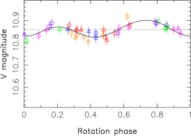
(a) 08b+09a

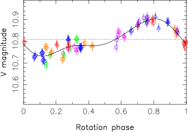
(b) 09b+10a

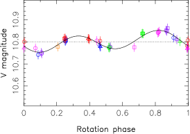
(c) 10b

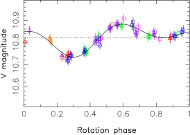
(d) 11b+12a

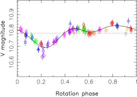
(e) 12b+13a

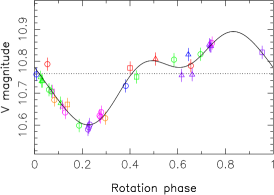
(f) 13b+14a

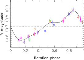
(g) 14b

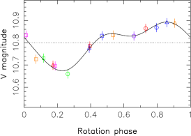
(h) 15b+16a

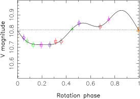
(i) 16b+17a

Figure 18: Fits of the V magnitude measurements at each epoch by a sine curve and two harmonics. Each data set was folded according to the corresponding period listed in Table 9. As a consequence, the rotation phase used in these plots does not correspond to the rotation phase in Table 7, but rather to the phase in the model sine curves.

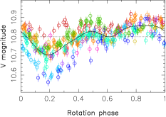
Figure 19: Fit of the V magnitude in the whole data set by a sine curve and four harmonics. The color-to-dataset correspondency is as follows: red=08b+09a, orange=09b+10a, yellow=10b, green=11b+12a, turquoise=12b+13a, cyan=13b+14a, blue=14b, purple=15b+16a, pink=16b+17a.

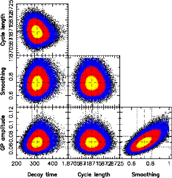
Figure 20: GPR-MCMC phase plot for the entire data set of V magnitudes. GP amplitude ${\theta_{1}=0.0712^{+0.0093}_{-0.0082}}$ mag, cycle length ${\theta_{2}=1.8715\pm 0.0003}$ d, decay time ${\theta_{3}=314^{+31}_{-29}}$ d, smoothing parameter ${\theta_{4}=0.74\pm 0.08}$ d.

Table 10: Results of the GPR-MCMC runs on our V magnitude measurements.

Data set	GP Period (d)	Decay time (d)	Smoothing (d)	Amplitude (mag)
	(best)	(best)	(best)	(best)
08b+09a	1.8693 $\pm$ 0.0014 (1.8694)	311.1333	0.7 $\pm$ 0.3 (0.5)	0.03${}^{+0.02}_{-0.01}$ (0.02)
09b+10a	1.8714 $\pm$ 0.0008 (1.8715)	311.1333	1.2 $\pm$ 0.3 (1.2)	0.12${}^{+0.05}_{-0.04}$ (0.11)
10b	1.8723 $\pm$ 0.0013 (1.8722)	311.1333	0.6 $\pm$ 0.2 (0.5)	0.04${}^{+0.03}_{-0.02}$ (0.03)
11b+12a	1.8704 $\pm$ 0.0007 (1.8705)	311.1333	1.0 $\pm$ 0.3 (0.7)	0.09${}^{+0.05}_{-0.03}$ (0.05)
12b+13a	1.8718 $\pm$ 0.0009 (1.8718)	311.1333	0.6 $\pm$ 0.2 (0.5)	0.06${}^{+0.03}_{-0.02}$ (0.04)
13b+14a	1.8721 $\pm$ 0.0008 (1.8722)	311.1333	0.7 $\pm$ 0.2 (0.6)	0.09${}^{+0.03}_{-0.02}$ (0.08)
14b	1.8735 $\pm$ 0.0012 (1.8732)	311.1333	0.6 $\pm$ 0.2 (0.5)	0.11${}^{+0.04}_{-0.03}$ (0.09)
15b+16a	1.8727 $\pm$ 0.0010 (1.8729)	311.1333	0.9 $\pm$ 0.3 (0.7)	0.08${}^{+0.03}_{-0.02}$ (0.06)
+16b+17a
All V mag	1.8715 $\pm$ 0.0003 (1.8714)	314${}^{+31}_{-29}$ (311.1333)	0.74 $\pm$ 0.08 (0.73)	0.071${}^{+0.009}_{-0.008}$ (0.070)

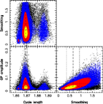
(a) 08b+09a

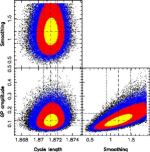
(b) 09b+10a

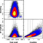
(c) 10b

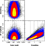
(d) 11b+12a

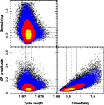
(e) 12b+13a

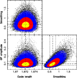
(f) 13b+14a

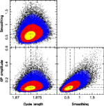
(g) 14b

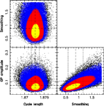
(h) 15b+16a+16b+17a

Figure 21: MCMC phase plots for GPR applied to each of our V magnitude data sets.

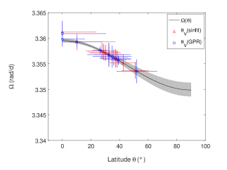
Figure 22: Differential rotation curve in blue, with parameters $\Omega_{\rm eq}$ and $d\Omega$ as defined in the introduction of Section 4. Red: H${\alpha}$ rotation rates, green: $B_{\rm\ell}$ rotation rates, circles: derived from 2013 Dec data set, triangles: derived from 2015 Dec data set, x symbols: derived from the whole data set (143 points for H${\alpha}$ and 135 for $B_{\rm\ell}$). Photometry rotation rates are displayed, those derived with sinfit (Table 9) in green and those derived with GPR (Table 10) in magenta.

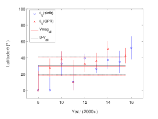
Figure 23: Colatitude found for the V magnitude, for each epoch and for the whole data set with sinfit (x-coordinate: 20) as well as for B-V with sinfit (x-coordinate: 21).

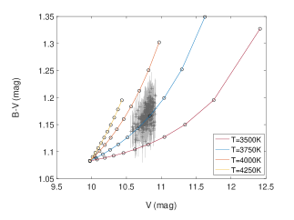
Figure 24: Fit of the B-V(V) curve with Kurucz models, with a photosphere temperature of 4500 K, $\log g$ of 3.5, E(B-V) of 0.10. Each full line corresponds to a particular value of the spot temperature, and dots mark the spot coverage with steps of 10% (the dot at V=10.0 and B-V=1.08 corresponding to a 0% spot coverage). The extension of our data correspond to a spot coverage constantly between 50% and 75%.

Appendix C Activity proxies

This section shows the line profiles of H${\alpha}$, He i and Ca ii, as well as some results on $B_{\rm\ell}$.

C.1 H$\alpha$

H$\alpha$ dynamic spectra are plotted in Figure 25, with the 2009 Jan data set being split in half to better see the absorption feature around phase 0.95. We also see two other absorption features in 2009 Jan around phase 0.80 and in 2011 Jan around phase 0.35, and we fit a sine curve in each to determine the potential altitude of a prominence or cloud that could be the origin of these absorption features. We find a sine semi-amplitude of $\sim$2 $v\sin i$ for each of them.

Lomb-Scargle periodograms for individual epochs are plotted in Figure 26, and the periodogram for the whole data set is shown in Figure 27, showing a neat peak at the rotation period.

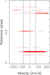
(a) 2008 Dec

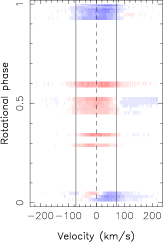
(b) 2009 Jan cycles 0-4

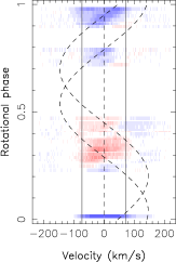
(c) 2009 Jan cycles 5-8

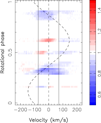
(d) 2011 Jan

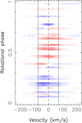
(e) 2013 Dec

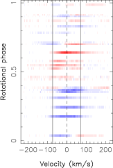
(f) 2015 Dec

(g) 2016 Jan

Figure 25: H${\alpha}$ dynamical spectra for epochs 2008 Dec (a), 2009 Jan (b,c), 2011 Jan (d), 2013 Dec (e), 2015 Dec (f) and 2016 Jan (g).

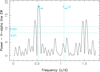
(a) 2009 Jan

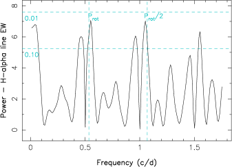
(b) 2011 Jan

Figure 26: Periodograms for the H${\alpha}$ line EW, for observation epochs 2009 Jan (a), 2011 Jan (b), 2013 Dec (c) and 2015 Dec (d). False-alarm probability levels of 1% and 0.1% are represented as horizontal cyan dashed lines, and $P_{\rm rot}$ and its first harmonic as vertical cyan dashed lines.

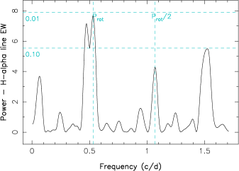
(c) 2013 Dec

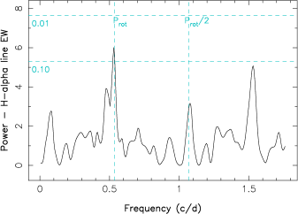
(d) 2015 Dec

Figure 26: (Continued from the previous page).

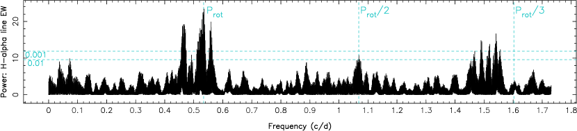
Figure 27: Periodogram of the equivalent width of the H${\alpha}$ line. The maximum power is found at 3.3636 rad/d, or 1.8680 d.

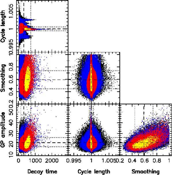
Figure 28: GPR-MCMC phase plot for our H${\alpha}$ equivalent width data. Amplitude ${\theta_{1}=21.4^{+4.7}_{-3.9}}$ km s^-1, decay time ${\theta_{3}=315^{+414}_{-179}}$ $P_{\rm rot}$, Cycle length ${\theta_{2}=1.0000\pm 0.0005}$ $P_{\rm rot}$, Smoothing ${\theta_{4}=0.59\pm 0.15}$ $P_{\rm rot}$.

C.2 He i $D_{3}$

The He i line profiles are shown in Fig. 29. We can clearly see the flares at the dates marked in Table 8.

(a) 2008 Oct

(b) 2008 Dec

(c) 2009 Jan

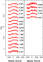
(d) 2011 Jan

(e) 2013 Nov

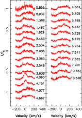
(f) 2013 Dec

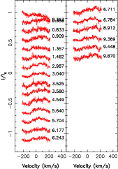
(g) 2015 Dec

(h) 2016 Jan

Figure 29: . He i $D_{3}$ Oct 2008 (ref cycle: -42), Dec 2008 (ref cycle: -15), Jan 2009 (ref cycle: 0), Jan 2011 (ref cycle: 397) Nov 2013 (ref cycle: 946), Dec 2013 (ref cycle: 959), Dec 2015 (ref cycle: 1349) and Jan 2016 (ref cycle: 1376)

C.3 Ca ii

The Ca ii line profiles are shown in Fig. 30.

(a) 2008 Oct

(b) 2008 Dec

(c) 2009 Jan

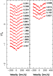
(d) 2011 Jan

(e) 2013 Nov

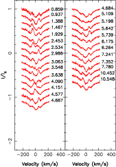
(f) 2013 Dec

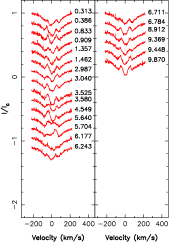
(g) 2015 Dec

(h) 2016 Jan

Figure 30: Ca ii $D_{3}$ Oct 2008 (ref cycle: -42), Dec 2008 (ref cycle: -15), Jan 2009 (ref cycle: 0), Jan 2011 (ref cycle: 397) Nov 2013 (ref cycle: 946), Dec 2013 (ref cycle: 959), Dec 2015 (ref cycle: 1349) and Jan 2016 (ref cycle: 1376)

C.4 $B_{\rm\ell}$

We derived longitudinal magnetic field values as first-order moments of our Stokes $V$ LSD profiles, and applied a GPR-MCMC run on them. The phase plot is shown in Figure 31.

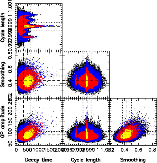
Figure 31: GPR-MCMC phase plot for $B_{\rm\ell}$. GP amplitude ${\theta_{1}=90^{+16}_{-14}}$ G, cycle length ${\theta_{2}=0.9989\pm 0.0004}$ $P_{\rm rot}$, decay time ${\theta_{3}=322^{+295}_{-154}}$ $P_{\rm rot}$, smoothing ${\theta_{4}=0.436\pm 0.066}$ $P_{\rm rot}$.

References

- Baraffe et al. (2015) Baraffe I., Homeier D., Allard F., Chabrier G., 2015, A&A, 577, A42
- Bouvier (2007) Bouvier J., 2007, in Bouvier J., Appenzeller I., eds, IAU Symposium Vol. 243, IAU Symposium. pp 231–240, doi:10.1017/S1743921307009593
- Bouvier & Bertout (1989) Bouvier J., Bertout C., 1989, A&A, 211, 99
- Bouvier et al. (2007) Bouvier J., Alencar S. H. P., Harries T. J., Johns-Krull C. M., Romanova M. M., 2007, in Reipurth B., Jewitt D., Keil K., eds, Protostars and Planets V. pp 479–494
- Brown et al. (1991) Brown S. F., Donati J.-F., Rees D. E., Semel M., 1991, A&A, 250, 463
- Carroll et al. (2012) Carroll T. A., Strassmeier K. G., Rice J. B., Künstler A., 2012, A&A, 548, A95
- Collier Cameron & Woods (1992) Collier Cameron A., Woods J. A., 1992, MNRAS, 258, 360
- Donati & Brown (1997) Donati J.-F., Brown S. F., 1997, A&A, 326, 1135
- Donati & Landstreet (2009) Donati J., Landstreet J. D., 2009, ARA&A, 47, 333
- Donati et al. (1997) Donati J.-F., Semel M., Carter B. D., Rees D. E., Collier Cameron A., 1997, MNRAS, 291, 658
- Donati et al. (2000) Donati J.-F., Mengel M., Carter B. D., Marsden S., Collier Cameron A., Wichmann R., 2000, MNRAS, 316, 699
- Donati et al. (2003) Donati J.-F., Collier Cameron A., Petit P., 2003, MNRAS, 345, 1187
- Donati et al. (2006) Donati J.-F., et al., 2006, MNRAS, 370, 629
- Donati et al. (2007) Donati J.-F., et al., 2007, MNRAS, 380, 1297
- Donati et al. (2008) Donati J.-F., et al., 2008, MNRAS, 386, 1234
- Donati et al. (2010a) Donati J., et al., 2010a, MNRAS, 402, 1426
- Donati et al. (2010b) Donati J., et al., 2010b, MNRAS, 409, 1347
- Donati et al. (2011) Donati J., et al., 2011, MNRAS, 412, 2454
- Donati et al. (2012) Donati J.-F., et al., 2012, MNRAS, 425, 2948
- Donati et al. (2013) Donati J.-F., et al., 2013, MNRAS, 436, 881
- Donati et al. (2014) Donati J.-F., et al., 2014, MNRAS, 444, 3220
- Donati et al. (2015) Donati J.-F., et al., 2015, MNRAS, 453, 3706
- Donati et al. (2016) Donati J. F., et al., 2016, Nature, 534, 662
- Donati et al. (2017) Donati J.-F., et al., 2017, MNRAS, 465, 3343
- Galli et al. (2018) Galli P. A. B., et al., 2018, ApJ, 859, 33
- Ghez et al. (1995) Ghez A. M., Weinberger A. J., Neugebauer G., Matthews K., McCarthy Jr. D. W., 1995, AJ, 110, 753
- Ghez et al. (1997) Ghez A. M., White R. J., Simon M., 1997, ApJ, 490, 353
- Grankin et al. (2008) Grankin K. N., Bouvier J., Herbst W., Melnikov S. Y., 2008, A&A, 479, 827
- Gregory et al. (2012) Gregory S. G., Donati J.-F., Morin J., Hussain G. A. J., Mayne N. J., Hillenbrand L. A., Jardine M., 2012, ApJ, 755, 97
- Gully-Santiago et al. (2017) Gully-Santiago M. A., et al., 2017, ApJ, 836, 200
- Hambálek et al. (2019) Hambálek Ä., VaÅko M., Paunzen E., Smalley B., 2019, MNRAS, 483, 1642
- Haywood et al. (2014) Haywood R. D., et al., 2014, MNRAS, 443, 2517
- Haywood et al. (2016) Haywood R. D., et al., 2016, MNRAS, 457, 3637
- Hébrard et al. (2016) Hébrard É. M., Donati J.-F., Delfosse X., Morin J., Moutou C., Boisse I., 2016, MNRAS, 461, 1465
- Hunter (2007) Hunter J. D., 2007, Computing in Science and Engineering, 9, 90
- Hussain et al. (2009) Hussain G. A. J., et al., 2009, MNRAS, pp 997–+
- Johns-Krull et al. (1999) Johns-Krull C. M., Valenti J. A., Koresko C., 1999, ApJ, 516, 900
- Kraus et al. (2011) Kraus A. L., Ireland M. J., Martinache F., Hillenbrand L. A., 2011, ApJ, 731, 8
- Kraus et al. (2012) Kraus A. L., Ireland M. J., Hillenbrand L. A., Martinache F., 2012, ApJ, 745, 19
- Kraus et al. (2016) Kraus A. L., Ireland M. J., Huber D., Mann A. W., Dupuy T. J., 2016, AJ, 152, 8
- Kurucz (1993) Kurucz R., 1993, CDROM # 13 (ATLAS9 atmospheric models) and # 18 (ATLAS9 and SYNTHE routines, spectral line database). Smithsonian Astrophysical Observatory, Washington D.C.
- Landi degl’Innocenti & Landolfi (2004) Landi degl’Innocenti E., Landolfi M., 2004, Polarisation in spectral lines. Dordrecht/Boston/London: Kluwer Academic Publishers
- Luhman et al. (2010) Luhman K. L., Allen P. R., Espaillat C., Hartmann L., Calvet N., 2010, ApJS, 186, 111
- Meunier et al. (2010) Meunier N., Desort M., Lagrange A.-M., 2010, A&A, 512, A39
- Morin et al. (2008) Morin J., et al., 2008, MNRAS, 390, 567
- Moutou et al. (2007) Moutou C., et al., 2007, A&A, 473, 651
- Pecaut & Mamajek (2013) Pecaut M. J., Mamajek E. E., 2013, ApJS, 208, 9
- Pollacco et al. (2006) Pollacco D. L., et al., 2006, PASP, 118, 1407
- Rice et al. (2011) Rice J. B., Strassmeier K. G., Kopf M., 2011, ApJ, 728, 69
- Siess et al. (2000) Siess L., Dufour E., Forestini M., 2000, A&A, 358, 593
- Skelly et al. (2010) Skelly M. B., Donati J.-F., Bouvier J., Grankin K. N., Unruh Y. C., Artemenko S. A., Petrov P., 2010, MNRAS, 403, 159
- Sokoloff et al. (2008) Sokoloff D. D., Nefedov S. N., Ermash A. A., Lamzin S. A., 2008, Astronomy Letters, 34, 761
- Stelzer et al. (2003) Stelzer B., et al., 2003, A&A, 411, 517
- Vaytet et al. (2018) Vaytet N., Commerçon B., Masson J., González M., Chabrier G., 2018, A&A, 615, A5
- Welty & Ramsey (1995) Welty A. D., Ramsey L. W., 1995, AJ, 110, 336
- Yadav et al. (2015) Yadav R. K., Christensen U. R., Morin J., Gastine T., Reiners A., Poppenhaeger K., Wolk S. J., 2015, ApJ, 813, L31
- Yu et al. (2017) Yu L., et al., 2017, MNRAS, 467, 1342