Incrementally Updated Spectral Embeddings

Abstract

Several fundamental tasks in data science rely on computing an extremal eigenspace of size $r\ll n$, where $n$ is the underlying problem dimension. For example, spectral clustering and PCA both require the computation of the leading $r$-dimensional subspace. Often, this process is repeated over time due to the possible temporal nature of the data; e.g., graphs representing relations in a social network may change over time, and feature vectors may be added, removed or updated in a dataset. Therefore, it is important to efficiently carry out the computations involved to keep up with frequent changes in the underlying data and also to dynamically determine a reasonable size for the subspace of interest. We present a complete computational pipeline for efficiently updating spectral embeddings in a variety of contexts. Our basic approach is to “seed” iterative methods for eigenproblems with the most recent subspace estimate to significantly reduce the computations involved, in contrast with a naïve approach which recomputes the subspace of interest from scratch at every step. In this setting, we provide various bounds on the number of iterations common eigensolvers need to perform in order to update the extremal eigenspace to a sufficient tolerance. We also incorporate a criterion for determining the size of the subspace based on successive eigenvalue ratios. We demonstrate the merits of our approach on the tasks of spectral clustering of temporally evolving graphs and PCA of an incrementally updated data matrix.

05C50, 65F10

1 Introduction

In the big data era, scientists and engineers need to operate on massive datasets on a daily basis, fueling essential algorithms for commercial or scientific applications. These datasets can contain millions or billions of data points, making the task of extracting meaningful information especially challenging [36]; moreover, it is often the case that the data are also high-dimensional, which can significantly affect the time and storage required to work with such datasets. These computational challenges strongly motivate the need to work with “summarized” versions of data that facilitate fast and memory-efficient computations. Several popular techniques in data science have been devised to address this problem, such as sketching [68], dimensionality reduction [4, 29, 54], and limited-memory/stochastic algorithms in optimization (see, e.g., [7] and references therein).

A popular approach to remedy some of the aforementioned difficulties revolves around using spectral information associated to the problem. For example, many high-dimensional problems involve data that can be modeled as graphs encoding interactions between entities in social networks [46], gene interaction data [45] and product recommendation networks [35]. A task of fundamental importance is clustering the nodes of the network into communities or clusters of similar nodes [50, 59]. Spectral clustering is a popular approach for this problem that computes the $r$ leading eigenvectors of the (symmetrically normalized) adjacency matrix, using this subspace as a low-dimensional representation of nodes in the graph, and then feeding this representation to a point cloud clustering algorithm such as k-means [43]. Determining $r$ on the fly is often done by comparing the ratios of successive eigenvalues [65].

In a similar vein, linear dimensionality reduction is often tackled via Principal Component Analysis (PCA) [29], which projects the data matrix $X$ to a low-dimensional coordinate system which is spanned by the leading eigenvectors of the covariance matrix, $X^{\top}X$. The $i$^th principal component is precisely the projection of the data matrix $X$ to the $i$^th eigenvector. In nonlinear dimensionality reduction, a common assumption is that the data lie on a low-dimensional manifold embedded in high-dimensional space. The method of Laplacian eigenmaps [6], which operates under this assumption, constructs a weighted adjacency matrix and solves a small sequence of eigenproblems to compute a lower-dimensional embedding of the data points.

1.1 Dealing with data that gets updated

Going one step further, many datasets get incrementally updated over time. For example, graph data can change in many ways: new links form between entities, old connections cease to exist, and new nodes are introduced to a network [64, 33]. In such cases, old clustering assignments may no longer accurately reflect the community structure of the network, and therefore need to be updated [44]. In other cases, the dimensionality of data may increase as more informative features as well as new data become available [5, 37]. Such updates reduce the fidelity of the previously computed low-dimensional embeddings. In both cases, we are faced with a pressing question: has the quality of the spectral embedding degraded, and if so, can we update it efficiently?

The main theoretical tools for answering the first part of this question come from matrix perturbation theory [61], which provides worst-case bounds for the distance between eigenspaces. However, algorithms proposed for updating spectral embeddings may not necessarily utilize those results. For example, if the original (unperturbed) data matrix and its updates are low rank, then one can update the thin SVD in practically linear time [8]; however, this is rarely the case in practice. Other “direct” approaches under low-rank updates are often inapplicable since they require the full set of singular values and vectors to be available for the unperturbed matrix [9, 26]. When the data matrix is sparse, a natural candidate may be updating the sparse Cholesky or $LDL^{\top}$ decompositions [12]; however, these rely on heuristics and may not necessarily preserve sparsity across multiple updates and it is unclear how to adapt these methods to maintain a low-dimensional subspace.

Several of the aforementioned approaches share a common prohibitive requirement: the knowledge of the full set of eigenvalues and eigenvectors at the beginning of an update step. If one is willing to forego guarantees on the accuracy of the updated embedding, it is at least empirically possible to exploit the first-order expansion of eigenvalues, where explicit knowledge of the full set is no longer required [44]. On the downside, this entails significant uncertainty about the quality of the maintained embedding. A more promising and relevant heuristic is that of warm-starting iterative eigenvalue methods. Many eigensolvers are typically initialized using a random guess, but when the target is a sequence of similar or related eigenproblems it is natural to expect that the previous solution might be a good initial estimate. This heuristic has been applied towards solving sequences of linear systems [31, 47], sometimes referred to as recycled Krylov method, and problems arising from successive linearizations of nonlinear eigenvalue problems [58].

Somewhat surprisingly, despite the empirical success of warm starting, it is often overlooked in favor of other heuristics [44] or matrix sketching to reduce per-iteration cost [25, 27].

1.2 Our contribution

Given the preceding discussion, an ideal method for incrementally computing spectral embeddings should:

1. incur minimal additional work per modification, ideally independent of the underlying problem’s dimension;

2. require minimal additional storage or extensive pre-computation (this excludes classical approaches that assume knowledge of the full set of eigenvalues [9]); and

3. take advantage of any features of the underlying matrix, such as sparsity or structure (e.g. Toeplitz matrices).

With regards to Item 1, it is important to be able to bound the amount of work required to update a spectral embedding on the fly, before performing the actual update.

In this paper, we show how warm-started iterative methods can naturally satisfy all of the above criteria under a minimal assumption on eigenvalue decay formalized in Section 3. We show that when the perturbations are “small”, using the previous subspace estimate as a “seed” for warm-starting entails essentially $\mathcal{O}(1)$ additional iterations per update even when the previous estimates have been computed inexactly (orders of magnitude above floating point error). We provide an adaptive algorithm for updating the spectral embedding over time as well computable bounds on the number of iterations required after each modification to the underlying matrix, for two standard iterative methods (eigensolvers). Because the main bottleneck operation of iterative methods is usually matrix-vector multiplication [18, 22, 57], the proposed algorithm naturally accelerates whenever the underlying matrix is structured or sparse. It also enables tracking a proxy for the appropriate subspace dimension, which can aid in determining the correct size of the spectral embedding on the fly.

In Section 4, we present a few concrete applications which fit into the incremental framework outlined above. In these settings, we are able to utilize properties of the perturbations to derive further a priori bounds on their effects on subspace distance. For example, when the perturbations are outer products of Gaussian random vectors, the subspace distance is affected by a factor of at most $\tilde{\mathcal{O}}\left(\sqrt{\frac{r}{n}}\right)$ with high probability. We also present experiments on real and synthetic data which validate the effectiveness of our approach.

Finally, we stress that we do not intend to provide a replacement to or compete with established eigensolvers, but rather describe a concrete pipeline for incremental spectral embeddings with well-understood worst-case guarantees. Indeed, our method only benefits from advances in software aimed at solving eigenproblems.

1.3 Notation

Throughout the paper, we endow $\mathbb{R}^{n}$ with the standard inner product $\left\langle x,y\right\rangle:=x^{\top}y$ and the induced norm $\left\|x\right\|_{2}=\sqrt{\left\langle x,x\right\rangle}$. Given a matrix $A\in\mathbb{R}^{n_{1}\times n_{2}}$ , we write $\left\|A\right\|_{2}$ for its spectral norm $\sup_{\left\|x\right\|_{2}=1}\left\|Ax\right\|_{2}$ and $\left\|A\right\|_{F}:=\sqrt{\mathrm{tr}(A^{\top}A)}$ for its Frobenius norm. We let $\mathbb{O}_{n,k}:=\left\{Q\in\mathbb{R}^{n\times k}\ \middle|\ Q^{\top}Q=I\right\}$ denote the set of real $n\times k$ matrices with orthonormal columns and drop the second subscript when $k=n$.

We write $\lambda_{i}(A)$ for the $i$^th eigenvalue of a matrix $A$, assuming a descending order such that $\lambda_{1}(A)\geq\dots\geq\lambda_{n}(A)$. We follow the same notation for singular values, $\sigma_{i}(A)$. Given a symmetric matrix $A\in\mathbb{R}^{n\times n}$, we will use its spectral decomposition:

(1) $$A=\begin{bmatrix}V&V_{\perp}\end{bmatrix}\begin{bmatrix}\Lambda&0\\ 0&\Lambda_{\perp}\end{bmatrix}\begin{bmatrix}V^{\top}\\ V_{\perp}^{\top}\end{bmatrix},$$

where $\begin{bmatrix}V&V_{\perp}\end{bmatrix}$ are the eigenvectors of $A$ and $\begin{bmatrix}\Lambda&0\\ 0&\Lambda_{\perp}\end{bmatrix}$ is a diagonal matrix containing the eigenvalues of $A$. By convention, $V$ should be understood to correspond to the subspace of interest. Similarly, when $A\in\mathbb{R}^{m\times n}$ with $m\geq n$ is an arbitrary rectangular matrix, we will use its singular value decomposition:

$$A=U\Sigma V^{\top}$$

where $U\in\mathbb{O}_{m,n},V\in\mathbb{O}_{n}$ are the left and right singular vectors of $A$ and $\Sigma$ is a diagonal matrix containing the singular values of $A$. We will write $\kappa(A):=\frac{\sigma_{1}(A)}{\sigma_{n}(A)}$ for $A$’s condition number. Throughout the main text, we refer to standard linear algebraic routines, which are built into numerical software packages such as LAPACK, using the following notation:

• $Q,R=\texttt{qr}(A)$ for the (reduced) QR factorization of $A\in\mathbb{R}^{m\times n}$ with $m\geq n$, which decomposes $A$ into an orthogonal matrix $Q\in\mathbb{O}_{m,n}$ and an upper triangular matrix $R\in\mathbb{R}^{n\times n}$.

• $V,\Lambda=\texttt{spectral}(A)$ for the spectral decomposition of a symmetric matrix $A\in\mathbb{R}^{n\times n}$, with $V$ containing the eigenvectors and $\Lambda:=\mathrm{diag}(\lambda_{1},\dots,\lambda_{n})$ containing the eigenvalues of $A$, respectively. We will assume that $\lambda_{1}\geq\dots\geq\lambda_{n}$ in $\Lambda$.

Moreover, we use $\mathrm{diag}(x_{1},\dots,x_{n})$ to refer to the diagonal matrix constructed from the vector $x=\begin{pmatrix}x_{1}&\dots&x_{n}\end{pmatrix}^{\top}$, and when $D$ is a matrix denote $\mathrm{diag}(D):=\begin{pmatrix}D_{11}&D_{22}&\dots&D_{nn}\end{pmatrix}^{\top}$. We also use notation from Golub and Van Loan [22] for matrix or vector slicing: $A_{:,1:r}$ denotes the submatrix of $A$ formed by taking the first $r$ columns, while $x_{1:r}$ denotes the vector formed by the leading $r$ elements of $x$.

2 Iterative Methods for Eigenvalue Problems

In this section we present two popular iterative methods for computing the eigenvalues of symmetric / Hermitian matrices that form the building blocks of our algorithms. Additionally, we review their convergence guarantees. Throughout, we assume that we are interested in the subspace corresponding to the algebraically largest eigenvalues (which are also the largest in magnitude, up to a shift). Recall that the Ritz values are the eigenvalues of the matrix ${V_{0}}^{\top}AV_{0}$, where $V_{0}$ is an approximation to an invariant subspace of $A$. Below, we are interested in subspace distances measured in the spectral norm, $\mathrm{dist}(V,\tilde{V}):=\left\|VV^{\top}-\tilde{V}\tilde{V}^{\top}\right\|_{2},$ which has been the focus of the convergence analysis of iterative methods for eigenproblems, and pairs well with established matrix perturbation theory for unitarily invariant norms.

Remark 1.

While our work predominantly relies on standard notions of subspace distance, many applications may benefit from different types of control over changes to invariant subspaces. In particular, controlling the $2\to\infty$ distance

$$\mathrm{dist}_{2\to\infty}(V,\tilde{V}):=\min_{W\in\mathbb{O}_{r}}\left\|V-\tilde{V}W\right\|_{2\to\infty}=\min_{W\in\mathbb{O}_{r}}\max_{j\in[n]}\left\|V_{j,:}-\tilde{V}_{j,:}W\right\|,$$

may be more applicable to settings where subspaces are interpreted row-wise (as is the case in spectral clustering). Recent work on perturbation theory for the $2\to\infty$ norm [1, 11, 15, 19] allows aspects our work to be extended to control incremental changes to the subspace under this metric. However, the lack of convergence theory for eigensolvers in this metric (beyond naïve bounds from norm equivalence) prevent us from performing a full analysis in this setting.

The eigensolvers sketched in Algorithms 1 and 2 perform a prescribed number of iterations $k_{\max}$. However, in practice one usually incorporates robust numerical termination criteria which often results in fewer iterations being required. We omit such criteria here to simplify the presentation and defer the details to the books by Parlett [48] and Saad [57].

Subspace iteration

Subspace iteration, also known as simultaneous iteration, is a well-studied generalization of the celebrated power method for computing the leading or trailing $r$ eigenvalues and eigenvectors of a symmetric matrix $A$. Starting from an initial guess $V_{0}$, the algorithm computes orthonormal bases for terms of the form $A^{q}V_{0}$, usually handled in practice via the QR factorization. In the special case of $r=1$, the intuition is that higher powers of $A$ amplify the component of the vector corresponding to the dominant eigenvector (as long as the initial guess is not perpendicular to that eigenvector). Since the estimates of subspace iteration converge to the eigenspace corresponding to eigenvalues of largest magnitude (instead of algebraically largest), we assume it will be used with an appropriate shift.

Algorithm 1 shows a full version of subspace iteration incorporating the Rayleigh-Ritz procedure. In the algorithm, $r$ stands for the desired number of eigenpairs sought, but we may opt for running it with a larger subspace of size $\ell>r$ for reasons that will be clarified later.

Algorithm 1 Subspace iteration

1:Input: matrix $A$, dimension $\ell$, target dimension $r$, initial estimate $V_{0}\in\mathbb{R}^{n\times\ell}$, $k_{\mathrm{max}}$.

2:for $k=1,\dots,k_{\max}$ do

3:     $V_{k},R_{k}:=\mathtt{qr}(AV_{k-1})$

4:     $Q_{k},\Lambda_{k}=\mathtt{spectral}({V_{k}}^{\top}AV_{k})$

5:     $V_{k}:=V_{k}\cdot Q_{k}$

6:end for

7:return $(V_{k})_{:,1:r},\mathrm{diag}(\Lambda_{k})_{1:r}$

There are a number of modifications (e.g., “locking” converged eigenpairs, shifts) that one can incorporate to improve subspace iteration in practice [57].

The following theorem characterizes the convergence of subspace iteration when $\ell=r$.

Theorem 2.1 (Adapted from Theorem 8.2.2 in [22]).

Consider the spectral decomposition of $A$ as in Eq. 1, assume that $\left|\lambda_{r}\right|>\left|\lambda_{r+1}\right|$, and let $d_{0}:=\left\|VV^{\top}-V_{0}V_{0}^{\top}\right\|_{2},\;\Delta_{0}:=\frac{d_{0}}{\sqrt{1-d_{0}^{2}}},$ where $V_{0}\in\mathbb{O}_{n,r}$. Then Algorithm 1 initialized with $V_{0}$ and $\ell=r$ produces an orthogonal matrix $V_{k}$ such that

(2) $$k_{\max}\geq\frac{\log(\Delta_{0}/\varepsilon)}{\log\left(\left|\frac{\lambda_{r}}{\lambda_{r+1}}\right|\right)}\Rightarrow\left\|VV^{\top}-V_{k}V_{k}^{\top}\right\|_{2}\leq\varepsilon.$$

The rate of convergence of individual eigenpairs may be faster than the rate implied by Theorem 2.1; for example, the rate of convergence of the $i$^th eigenvalue estimate is asymptotically $\mathcal{O}(\left|\lambda_{i}/\lambda_{r+1}\right|)$ [60].

The amount of work suggested by Theorem 2.1 crucially relies on two quantities: the eigenvalue ratio $\rho:=\frac{\lambda_{r}}{\lambda_{r+1}}$, which controls the convergence rate, as well as the initial subspace distance $d_{0}$. In this paper, we use the fact that even if $\rho$ is moderately close to $1$, a small initial distance can result in fewer iterations.

Block Krylov method

Subspace iteration, while practical, discards a lot of useful information by only using the last computed power $A^{q}V_{0}$, instead of using the full (block) Krylov subspace $\mathrm{span}(V_{0},AV_{0},\dots,A^{q}V_{0})$. This is precisely the motivation for (block) Krylov methods. The well-known Lanczos method is part of this family when $V_{0}=v_{0}$, a single vector. In practice, the Lanczos method often exhibits superlinear convergence [48, 55], making it the method of choice for eigenvalue computation. However, its performance deteriorates in the presence of repeated or clustered (i.e., very close to each other in magnitude) eigenvalues. It is well-known that the single-vector Lanczos method cannot find multiple eigenvalues without deflation [57] and converges slowly for clustered eigenvalues. On the other hand, the block Lanczos method can get around this issue, provided the block size $b$ is set appropriately (i.e., $b>r$). See Parlett [48] for a discussion on the tradeoffs of block sizes.

Algorithm 2 presents a Block Krylov method, albeit an impractical variant as it forms the full Krylov matrix. While far from a practical implementation, this form is helpful for stating and interpreting results under the assumption that we are operating in exact arithmetic.

Algorithm 2 Block Krylov method

1:Input: $A\in\mathbb{R}^{n\times n}$, dimension $r$, block size $b\geq r$, initial matrix $V_{0}\in\mathbb{R}^{n\times b}$, power $k_{\max}$.

2:Form the block Krylov matrix

$$K=\begin{bmatrix}AV_{0}&(AA^{\top})AV_{0}&\dots&(AA^{\top})^{k_{\max}}AV_{0}\end{bmatrix}$$

3:$Q,R=\mathtt{qr}(K)$

4:$V_{k},\Lambda_{k}=\mathtt{spectral}(Q^{\top}AQ)$

5:return $(QV_{k})_{:,1:r},\mathrm{diag}(\Lambda_{k})_{1:r}$

The block Lanczos algorithm first appeared to address the shortcomings of the single-vector Lanczos iteration [14]. Saad provides a comprehensive convergence analysis [56], while more recent work presents sharp bounds and addresses convergence to clusters of eigenvalues [39]. For our purposes, we use the analysis found in Wang et al. [66], the results of which are stated in a form easily comparable with the corresponding rate for Algorithm 1.

Theorem 2.2 (Adapted from Theorem 6.6 in [66]).

Consider the Schur decomposition of $A$ as in Eq. 1, assume that $\lambda_{r}>\lambda_{r+1}$, and let $d_{0}:=\left\|VV^{\top}-V_{0}V_{0}^{\top}\right\|_{2},\;\Delta_{0}:=\frac{d_{0}}{\sqrt{1-d_{0}^{2}}}$, where $V_{0}\in\mathbb{O}_{n,r}$. Then Algorithm 2 initialized with $V_{0}$ produces an orthogonal matrix $V_{k}$ such that

(3) $$k_{\max}\geq\frac{1+\log_{2}(\Delta_{0}/\varepsilon)}{\sqrt{\left|\frac{\lambda_{r}}{\lambda_{r+1}}\right|-1}}\Rightarrow\left\|VV^{\top}-V_{k}{V_{k}}^{\top}\right\|_{2}\leq\varepsilon.$$

Comparing with the rate of Theorem 2.1, the block Lanczos method is clearly superior to subspace iteration: in the challenging regime where $\lambda_{r}\approx\lambda_{r+1}$, $\sqrt{\frac{\lambda_{r}}{\lambda_{r+1}}-1}\gg\log\left(\frac{\lambda_{r}}{\lambda_{r+1}}\right)$. As with Algorithm 1, it is important to keep in mind that starting from an estimate $V_{0}$ with $d_{0}\ll 1$ can result in a significant reduction of the required number of iterations.

3 Subspace estimation with incremental updates

In this section, we develop our incremental approach to spectral estimation, motivated by data that changes over time. As stated before, we are interested in maintaining an invariant subspace across “small” modifications to the data. More specifically, we have a matrix $A\in\mathbb{R}^{n\times n}$ and wish to dynamically update an estimate of the leading invariant subspace of $A$ corresponding to the eigenvalues of largest magnitude. This is not without loss of generality; for example, modifying subspace iteration for finding the smallest eigenpairs involves solving a linear system. However, some applications stated in terms of finding the smallest eigenpairs can be reformulated to fit our setting (see Section 4.1). A common example of such a problem is spectral clustering for community detection in graphs, which we rely on for intuition and constructing various numerical examples in the experimental section. However, our approach generalizes beyond the graph setting.

We formalize the incremental updates to our matrix as follows:

Assumption 1.

Let $A_{(0)}:=A\in\mathbb{R}^{n\times n}$. At each time step $t\in\left\{1,\dots,T\right\}$, we observe updates of the form $A_{(t)}:=A_{(t-1)}+E_{(t)}$, where $E_{(t)}$ is random, sparse, or low-rank. We denote the eigenvectors and eigenvalues of $A_{(t)}$ by $V_{(t)}$ and $\Lambda_{(t)}$.

An additional assumption that we impose on our matrix $A$ is that there is sufficient decay on the lower end of the spectrum outside of the subspace of interest, stated as 2.

Assumption 2.

Let $\lambda_{1}\geq\lambda_{2}\geq\dots\geq\lambda_{n}$ be the ordered eigenvalues of $A$. There is a constant $\gamma>0$ and an integer $r_{0}\ll n$ such that $\forall r\leq r_{0}$, there exists a $p\ll n$ satisfying

(4) $$\left|\lambda_{r}\right|\geq(1+\gamma)\left|\lambda_{p}\right|.$$

Intuitively, 2 implies a sort of “uniform” decay on the eigenvalues of $A$, since $\gamma$ does not depend on the particular choice of $r\leq r_{0}$. Indeed, if we allowed $\gamma=0$, then Eq. 4 would be trivially satisfied. The challenging regime is when $\gamma\ll 1$, as hinted by standard convergence results on iterative methods for eigenvalue problems [18, 22, 57].

This technical assumption allows us to derive a priori upper bounds on the required steps of our eigensolvers discussed above. In all the experiments presented in Section 4, 2 was verified to hold with $\gamma>0.1$ and $p\leq r+10$.

3.1 Outline of our approach

We now sketch the high-level idea behind our approach. Naturally, not all modifications to the underlying data have the same effect on the invariant subspace of interest. For instance, “small” (with respect to some matrix norm) modifications should not significantly change the leading eigenvalues and eigenvectors. Matrix perturbation theory provides us with the analytical tools to measure the worst-case behavior of these modifications [61]. Intuitively, if this behavior is sufficiently “bounded”, seeding our iterative method at the previously obtained estimate should reduce the computation required to obtain the next estimate. This is the crux of our approach.

An indispensable tool for perturbation bounds is the Davis–Kahan theorem [16, 38]. In order to state it formally, we first recall the definition of principal angles between subspaces [61].

Definition 3.1.

Consider matrices $V,W\in\mathbb{O}_{n,k}$ and their corresponding column spaces $\mathcal{V},\mathcal{W}$. Denote $\sigma_{i}:=\sigma_{i}(V^{\top}W),\;i=1,\dots,k$. The principal angles between $\mathcal{V}$ and $\mathcal{W}$ are the diagonal elements of the matrix

$$\Theta(V,W):=\mathrm{diag}(\cos^{-1}\sigma_{1},\dots,\cos^{-1}\sigma_{k}).$$

Moreover, the $\sin$-distance between $\mathcal{V},\mathcal{W}$ for any unitarily invariant norm $\left\|\cdot\right\|$ is

(5) $$\left\|\sin\Theta(V,W)\right\|:=\left\|\mathrm{diag}\left(\sin(\cos^{-1}\sigma_{1}),\dots,\sin(\cos^{-1}\sigma_{k})\right)\right\|.$$

With Definition 3.1 in hand, we can state the Davis–Kahan Theorem 3.2. While it holds for any unitarily invariant norm, we are only interested in the case where $\left\|\cdot\right\|=\left\|\cdot\right\|_{2}$.

Theorem 3.2 (Davis–Kahan).

Suppose $A,\hat{A}$ are symmetric and let $V,\hat{V}\in\mathbb{R}^{n\times r}$ be two invariant subspaces containing eigenvectors of $A$ and $\hat{A}$, respectively. Let $\Lambda(V)$ denote the set of eigenvalues of $A$ corresponding to $V$ and $\Lambda(\hat{V}_{\perp})$ the set of eigenvalues of $\hat{A}$ corresponding to $\hat{V}_{\perp}$. If there exists an interval $[\alpha,\beta]$ and $\delta>0$ such that $\Lambda(V)\in[\alpha,\beta]$ and $\Lambda(\hat{V}_{\perp})\in(-\infty,\alpha-\delta)\cup(\beta+\delta,+\infty)$, then

(6) $$\left\|\sin\Theta(V,\hat{V})\right\|_{2}\leq\frac{\left\|(\hat{A}-A)V\right\|_{2}}{\delta}.$$

Moreover, if $\left\|A-\hat{A}\right\|_{2}<\frac{\delta_{r}}{2}$, where $\delta_{r}=\min\left\{\left|\mu-\lambda\right|\ \middle|\ \mu\in\Lambda(V_{\perp}),\lambda\in\Lambda(V)\right\}$, then

(7) $$\left\|\sin\Theta(V,\hat{V})\right\|_{2}\leq\frac{2\left\|(\hat{A}-A)V\right\|_{2}}{\delta_{r}}.$$

Equation 7 above is straightforward to derive (e.g., see the proof of [21, Corollary 2.1]). We employ Theorem 3.2 to obtain an a priori bound on the distance between previously available subspace estimates and the invariant subspace of the updated matrix. Algorithm 3 outlines our high-level strategy.

Algorithm 3 High-level algorithm for subspace updates

1:Input: Matrix $A:=A_{(0)}$, initial subspace size $r$, high-order $q\geq 1$, threshold $\varepsilon$.

2:$\triangleright$ compute estimates $\hat{V}_{(0)}\in\mathbb{R}^{n\times r}$ and $\hat{\lambda}_{r},\dots,\hat{\lambda}_{r+q}$.

3:for $t=1,\dots,T$ do

4:     $A_{(t)}:=A_{(t-1)}+E_{(t)}$

5:     $\bullet$ estimate $\left\|\sin\Theta(V_{(t)},V_{(t-1)})\right\|_{2}\leq d_{t}$ $\triangleright$ Section 3.2.3

6:     if $d_{t}>\varepsilon$ then

7:         $\bullet$ update $\hat{V}_{(t)},\hat{\lambda}_{r}$ to tolerance $\varepsilon$ $\triangleright$ Section 3.2.1

8:         $\bullet$ update high order eigenvalues $\hat{\lambda}_{r+1},\dots,\hat{\lambda}_{r+q}$ to tolerance $\varepsilon$ $\triangleright$ Section 3.2.2

9:         $\bullet$ update subspace size $r$ $\triangleright$ Section 3.2.4

10:     end if

11:end for

In Algorithm 3, the constant $q\geq 1$ is an “oversampling” factor which is utilized as a heuristic for updating the size of the subspace on the fly as well as for estimating the convergence rate $\lvert\frac{\lambda_{r}}{\lambda_{r+1}}\rvert$ for our choice of eigenvalue algorithm. Step 7 updates the subspace estimate while step 8 updates the higher order eigenvalue estimates. These updates are triggered when our proxy for Eq. 7 is above a specified threshold $\varepsilon$.

Remark 3.3 (Extension for singular subspaces).

Our method is easily adapted for computing the leading singular subspace of a rectangular matrix $A\in\mathbb{R}^{m\times n}$. Via the standard dilation trick [22, 61], we can form

$$S=\begin{pmatrix}0&A\\ A^{\top}&0\end{pmatrix}\Rightarrow\lambda_{i}(S)=\pm\sigma_{i}(A),$$

and given the (thin) SVD of $A$, $A=U\Sigma V^{\top}$, it is easy to verify that the $i$^th eigenvector of $S$ is the concatenation of the $i$^th left and right singular vectors, $u_{i}$ and $v_{i}$. Alternatively, if one is interested only in the left or right singular subspace, it is also possible to run Algorithm 3 on $A^{\top}A$ or $AA^{\top}$ implicitly, without ever forming the complete matrix—at the expense of standard conditioning consequences.

3.2 Detailed description

Below, we describe how to efficiently implement each of the aforementioned steps, addressing the fact that our estimates at each step are inexact. We discuss $d_{t}$ last, focusing on the updates in lines 7 and 8 of Algorithm 3 first.

3.2.1 Computing the new subspace

Let us first assume that $d_{t}$ from step 5 has already been computed. Given the previous subspace estimate $\hat{V}_{(t-1)}\in\mathbb{R}^{n\times r}$, we can seed our eigensolver (Algorithm 1 or Algorithm 2) with $\hat{V}_{(t-1)}$. Assume that

$$\left|\hat{\lambda}_{r}(A_{(t-1)})-\lambda_{r}(A_{(t-1)})\right|\leq\varepsilon_{1},\;\left|\hat{\lambda}_{r+1}(A_{(t-1)})-\lambda_{r+1}(A_{(t-1)})\right|\leq\varepsilon_{2}.$$

Applying Weyl’s inequality (Lemma A.7), the rate controlling convergence will be at least

(8) $$\frac{\lambda_{r}(A_{(t)})}{\lambda_{r+1}(A_{(t)})}\geq\frac{\lambda_{r}(A_{(t-1)})-\left\|E_{(t)}\right\|_{2}}{\lambda_{r+1}(A_{(t-1)})+\left\|E_{(t)}\right\|_{2}}\geq\frac{\hat{\lambda}_{r}-\left\|E_{(t)}\right\|_{2}-\varepsilon_{1}}{\hat{\lambda}_{r+1}+\left\|E_{(t)}\right\|_{2}+\varepsilon_{2}}=:\rho_{t},$$

and Theorems 2.1 and 2.2 say that we have to set (with $\Delta_{t}:=d_{t}/\sqrt{1-d_{t}^{2}}$):

(9) $$k_{\max}\geq\begin{cases}\frac{\log\left(\Delta_{t}/\varepsilon\right)}{\log(\rho_{t})}&\text{ for \lx@cref{creftypecap~refnum}{alg:subspace-iter}}\\[5.69054pt] \frac{1+\log_{2}\left(\Delta_{t}/\varepsilon\right)}{\sqrt{\rho_{t}-1}}&\text{ for \lx@cref{creftypecap~refnum}{alg:block-krylov}}\end{cases}$$

in order to guarantee $\mathrm{dist}(V_{(t)},\hat{V}_{(t)})\leq\varepsilon$.

In order to set $k_{\max}$, we need to know the error bounds $\varepsilon_{1}$ and $\varepsilon_{2}$ on the accuracy of the previously computed eigenvalues $\hat{\lambda}_{r}$ and $\hat{\lambda}_{r+1}$. For $\hat{\lambda}_{r}$, we can apply Theorem A.6 for the estimate $\hat{V}_{(t-1)}$ which gives us

(10) $$\left|\hat{\lambda}_{r}(A_{(t-1)})-\lambda_{r}(A_{(t-1)})\right|\leq\rho(A_{(t-1)})\left\|\sin\Theta(\hat{V}_{(t-1)},V_{(t-1)})\right\|_{2}^{2}\leq\rho(A_{(t-1)})\varepsilon^{2}.$$

For the higher order eigenvalue estimate $\hat{\lambda}_{r+1}$, we can deduce a similar worst-case bound (see Section 3.2.2 for details):

(11) $$\left|\hat{\lambda}_{r+1}(A_{(t-1)})-\lambda_{r+1}(A_{(t-1)})\right|\leq 2\rho(A_{(t-1)})\varepsilon^{2}.$$

In Eq. 11, the error factor is due to the combined inexactness of the “deflated” matrix and the estimate returned from the iterative method of choice.

3.2.2 Computing the higher order eigenvalues

The best way for updating the higher order eigenvalue estimates $\hat{\lambda}_{r+1},\dots$, $\hat{\lambda}_{r+q}$ is not obvious. One possible approach is to “augment” the tracked subspace updated at Line 7 to have dimension $r+q$. However, because iterative eigenvalue algorithms use some orthogonalization scheme (e.g., QR factorization) that scales quadratically in the subspace dimension [22], we would have incurred a cost proportional to (at least) $(r+q)^{2}$.

A more careful approach is a 2-phase algorithm, where we lock the $r$-dimensional estimate ${\hat{{V}}_{({t})}}$ and apply an iterative method to the “deflated” matrix $(I-{\hat{{V}}_{({t})}}{\hat{{V}}_{({t})}}^{\top})A_{(t)}(I-{\hat{{V}}_{({t})}}{\hat{{V}}_{({t})}}^{\top})$, with potentially substantially smaller time and memory costs than would be required for maintaining an $(r+q)$-dimensional subspace. Even though it is evident that deflating $A_{(t)}$ this way must incur some loss of accuracy, by Lemma 3.4 this loss is negligible when $\varepsilon\leq\rho(A_{(t)})^{-1}$.

Lemma 3.4.

Consider a matrix $A=\begin{bmatrix}V&V_{\perp}\end{bmatrix}\begin{bmatrix}\Lambda&0\\ 0&\Lambda_{\perp}\end{bmatrix}\begin{bmatrix}V&V_{\perp}\end{bmatrix}^{\top}$ and an estimate $\widehat{V}\in\mathbb{O}_{n,r}$ such that $\left\|VV^{\top}-\widehat{V}{\widehat{V}}^{\top}\right\|_{2}\leq\varepsilon$. Then

(12) $$\left|\lambda_{r+i}(A)-\lambda_{i}\left((I-\widehat{V}{\widehat{V}}^{\top})A(I-\widehat{V}{\widehat{V}}^{\top})\right)\right| \leq\rho(A)\varepsilon^{2}$$

Proof 3.5.

If $V$ contains a basis for the leading $r$-dimensional eigenspace, then it is obvious that $I-VV^{\top}$ is the projector to the trailing $(n-r)$-dimensional eigenspace, which corresponds to a contiguous set of eigenvalues of $A$. By elementary arguments, we know that

$$\lambda_{r+i}(A)=\lambda_{i}\big{(}\underbrace{(I-VV^{\top})A(I-VV^{\top})}_{=:\tilde{A}}\big{)}.$$

Therefore, by Theorem A.6,

$$\max_{i}\left|\lambda_{i}\left(\tilde{A}\right)-\lambda_{i}\left((I-\widehat{V}{\widehat{V}}^{\top})A(I-\widehat{V}{\widehat{V}}^{\top})\right)\right|\leq\rho(A)\left\|VV^{\top}-\widehat{V}{\widehat{V}}^{\top}\right\|_{2}^{2}\leq\rho(A)\varepsilon^{2},$$

since $(I-\widehat{V}{\widehat{V}}^{\top})$ is also a projector to an $(n-r)$-dimensional subspace.

We conclude the following accuracy estimate (dropping the $(t)$ subscript for brevity):

(13) $$\begin{aligned} \left|\lambda_{r+i}(A)-\hat{\lambda}_{r+i}(A)\right|&\leq\left|\lambda_{r+i}(A)-\lambda_{i}\left((I-\hat{V}\hat{V}^{\top})A(I-\hat{V}\hat{V}^{\top})\right)\right|\\ &\quad+\left|\lambda_{i}\left((I-\hat{V}\hat{V}^{\top})A(I-\hat{V}\hat{V}^{\top})\right)-\hat{\lambda}_{i}\left((I-\hat{V}\hat{V}^{\top})A(I-\hat{V}\hat{V}^{\top})\right)\right|\\ &\leq 2\rho(A)\varepsilon^{2}\end{aligned},$$

with the first $\rho(A)\varepsilon^{2}$ factor coming from an application of Lemma 3.4 and the second such factor coming from an application of Theorem A.6 when applying our iterative method with accuracy parameter $\varepsilon$ to the deflated matrix. This provides the inequality in Eq. 11.

When computing higher order eigenvalues, we might not have a previously maintained estimate of the corresponding subspace. In this situation, it is common to pick a random Gaussian matrix as the seed matrix. The two following Propositions provide guarantees for Algorithms 1 and 2 under this initialization scheme.

Proposition 3.6 (Corollary of Theorem 5.8 in [25]).

Let $A=V\Lambda V^{\top}$ be a symmetric matrix, and let $0\leq p\leq\ell-k$. For a given $\delta\in(0,1)$, define

$$C_{\delta}:=\frac{e\sqrt{\ell}}{p+1}\left(\frac{2}{\delta}\right)^{\frac{1}{p+1}}\left[\sqrt{n-\ell+p}+\sqrt{\ell}+\sqrt{2\log\left(\frac{2}{\delta}\right)}\right].$$

Then, with probability at least $1-\delta$, for $j=1,\dots,k$, the Ritz values $\left\{\mu_{j}\right\}$ returned by Algorithm 1 initialized with a random Gaussian matrix $(V_{0})_{ij}\sim\mathcal{N}(0,1)$ satisfy

$$\lambda_{j}\geq\mu_{j}\geq\frac{\lambda_{j}}{\sqrt{1+C_{\delta}^{2}\left(\frac{\lambda_{\ell-p+1}}{\lambda_{j}}\right)^{4k_{\max}+2}}},\quad\forall j=1,\dots,r.$$

Proposition 3.7 (Theorem III.4 in [69]).

Let $A=V\Lambda V^{\top}$ be a symmetric matrix, and let $b=r+p$ in Algorithm 2 initialized with $(V_{0})_{ij}\sim\mathcal{N}(0,1)$. Then, for $j=1,\dots,r$, the Ritz values $\left\{\mu_{j}\right\}$ returned satisfy

$$\lambda_{j}\geq\mu_{j}\geq\frac{\lambda_{j}}{\sqrt{1+C^{2}T_{2k_{\max}+1}^{-2}\left(1+2\frac{\lambda_{j}-\lambda_{j+p+1}}{\lambda_{j+p+1}}\right)}},$$

where $T_{p}$ is the $p$^th degree Chebyshev polynomial and $C$ is a constant depending on the initialization matrix.

Let us incorporate 2 into Propositions 3.6 and 3.7. For the latter, it is known that Chebyshev polynomials satisfy $T_{d}(1+\alpha)\geq 2^{d\sqrt{\alpha}}$ when $\alpha\ll 1$ (see [42, Lemma 5]). Therefore, to achieve $\varepsilon$-accuracy under Gaussian initialization, we can set

(14) $$k_{\max}\geq\begin{cases}\frac{\log(C_{1}/\varepsilon)}{\log(1+\gamma)}&\text{ for \lx@cref{creftype~refnum}{alg:subspace-iter}}\\[5.69054pt] \frac{\log(C_{2}/\varepsilon)}{\sqrt{\gamma}}&\text{ for \lx@cref{creftype~refnum}{alg:block-krylov}},\end{cases}$$

where $C_{1},C_{2}$ are the constants from Propositions 3.6 and 3.7.

3.2.3 A proxy for the Davis–Kahan bound

We still need a good bound $d_{t}$ on the subspace distance in Eq. 7. Evaluating $\left\|(A_{(t)}-A_{(t-1)})V\right\|_{2}$ exactly is not possible, since we only maintain approximations of $V$. A standard majorizer, often too loose in practice, is $\left\|A_{(t)}-A_{(t-1)}\right\|_{2}$. We can get a better upper bound by leveraging a priori information about the perturbation, such as sparsity or randomness—two such instances are handled in Section 4.

We can still get around this issue in the absence of prior information about $E_{(t)}=A_{(t)}-A_{(t-1)}$. Let us first assume that we have computed a $\varepsilon$-close subspace estimate ${\hat{{V}}_{({t})}}$ (i.e., $\mathrm{dist}(V_{(t)},{\hat{{V}}_{({t})}})\leq\varepsilon$ ). Given this information, we can compute an upper bound to the subspace distance at time $t+1$ in terms of ${\hat{{V}}_{({t})}}$ and the perturbation $E_{(t)}$, as Lemma 3.8 shows. Again, we drop the subscripts for simplicity.

Lemma 3.8.

Let $E$ be a perturbation to a matrix $A=\begin{bmatrix}V&V_{\perp}\end{bmatrix}\Lambda\begin{bmatrix}V&V_{\perp}\end{bmatrix}^{\top}$ and $\widehat{V}$ be a subspace estimate such that $\left\|VV^{\top}-\widehat{V}{\widehat{V}}^{\top}\right\|_{2}\leq\varepsilon.$ Then

(15) $$\left\|EV\right\|_{2} \leq\sqrt{\left\|E\widehat{V}\right\|^{2}_{2}+\varepsilon\left\|E\right\|^{2}_{2}}.$$

Proof 3.9.

Using the triangle inequality for the first inequality and our assumption on $V,\hat{V}$ for the second inequality, we obtain

$$\left\|EV\right\|_{2} \leq\sqrt{\left\|E(VV^{\top}-\widehat{V}{\widehat{V}^{\top}})E^{\top}\right\|_{2}+\left\|E\widehat{V}{\widehat{V}}^{\top}E^{\top}\right\|_{2}}\leq\sqrt{\varepsilon\left\|E\right\|^{2}_{2}+\left\|E\widehat{V}\right\|_{2}^{2}}.$$

This provides us with a proxy for the numerator of Eq. 6, with the estimate for the eigenvalue gap following from the discussion in Sections 3.2.1 and 3.2.2. From Eqs. 10 and 11, we know that the approximate eigengap $\hat{\delta}_{r}:=\hat{\lambda}_{r}-\hat{\lambda}_{r+1}$ satisfies

$$\left|\hat{\delta}_{r}-\delta_{r}\right| =\left|\lambda_{r}({V_{0}}^{\top}AV_{0})-\lambda_{1}((I-V_{0}{V_{0}}^{\top})A(I-V_{0}{V_{0}}^{\top}))\right|\leq 3\varepsilon^{2}\rho(A).$$

Putting everything together, we arrive at Corollary 3.10, whose proof follows immediately after applying Lemma 3.8 to bound the numerator on Theorem 3.2.

Corollary 3.10.

Given a sequence of updates satisfying 1, Algorithm 3 maintains an estimate $\widehat{V}_{(t)}$ satisfying $\mathrm{dist}(\widehat{V}_{(t)},V_{(t)})\leq\varepsilon$. If $\left|\lambda_{r}(A_{(t-1)})-\lambda_{r+1}(A_{(t-1)})\right|<\frac{\left\|E_{(t)}\right\|_{2}}{2}$, Line 7 of Algorithm 3 takes at most $k_{\max}$ iterations, with

(16) $$k_{\max}\geq\begin{cases}\frac{\log(\Delta_{t}/\varepsilon)}{\log(\rho_{t})}&\text{ for \lx@cref{creftype~refnum}{alg:subspace-iter}}\\[5.69054pt] \frac{1+\log(\Delta_{t}/\varepsilon)}{\sqrt{\rho_{t}-1}}&\text{ for \lx@cref{creftype~refnum}{alg:block-krylov},}\end{cases}$$

where $\Delta_{t}:=\frac{d_{t}}{\sqrt{1-d_{t}^{2}}}$ and $\left\{d_{t},\rho_{t}\right\}$ are given by

(17) $$\begin{aligned} d_{t}&:=\frac{2\sqrt{\varepsilon\left\|E_{(t)}\right\|^{2}_{2}+\left\|E_{(t)}\widehat{V}_{(t-1)}\right\|^{2}_{2}}}{\hat{\lambda}_{r}(A_{(t-1)})-\hat{\lambda}_{r+1}(A_{(t-1)})-3\varepsilon^{2}\rho(A_{(t-1)})}\\ \rho_{t}&:=\frac{\hat{\lambda}_{r}(A_{(t-1)})-\left\|E_{(t)}\right\|_{2}-\rho(A_{(t-1)})\varepsilon^{2}}{\hat{\lambda}_{r+1}(A_{(t-1)})+\left\|E_{(t)}\right\|_{2}+2\rho(A_{(t-1)})\varepsilon^{2}}.\end{aligned}$$

Moreover, under 2, Line 8 takes at most $k_{\max}^{\prime}$ iterations, with

(18) $$k_{\max}^{\prime}\geq\begin{cases}\frac{\log(C_{1}/\varepsilon)}{\log(1+\gamma)}&\text{ for \lx@cref{creftype~refnum}{alg:subspace-iter}}\\[5.69054pt] \frac{\log(C_{2}/\varepsilon)}{\sqrt{\gamma}}&\text{ for \lx@cref{creftype~refnum}{alg:block-krylov},}\end{cases}$$

where $C_{1},C_{2}$ are the constants in Propositions 3.6 and 3.7.

Remark 3.11.

Though the factor $\rho(A)$ above seems to introduce a non-negligible loss, several applications of interest satisfy $\rho(A)=\mathcal{O}(\varepsilon^{-1})$. For example, spectral clustering with the normalized adjacency matrix satisfies $\rho(A)\leq 2$. On the numerical side, if we can’t assume that $\rho(A)=\mathcal{O}(\varepsilon^{-1})$, it is sometimes possible to estimate $\rho(A_{(t)})\leq\hat{\lambda}_{1}({\hat{{A}}_{({t-1})}})+\left\|E_{(t)}\right\|_{2}$ using Lemma A.7, as in the case of positive semi-definite matrices. This task is straightforward in all applications considered in Section 4.

If the assumption of the Davis-Kahan theorem fails or $d_{t}\geq 1$, it is straightforward to check that seeding with a Gaussian matrix results in the bound of Eq. 18 for Line 7, with $\rho_{t}$ instead of $\gamma$ if $\rho_{t}>1$.

3.2.4 Subspace size updates

As discussed in Section 1.1, it is often the case that the dimension $r$ of the subspace of interest is either not known a priori or changing over time. In spectral clustering, a common heuristic to determine the “correct” size of clusters is to compute a large extremal eigenspace of the normalized adjacency matrix and observe the ratios of successive eigenvalues [65].

We can extend this criterion to enable tracking the dimension over time, as approximating higher order eigenvalues given an $r$-dimensional invariant subspace is feasible via the procedure described in Lemma 3.4. Assume that estimates $\hat{\lambda}_{1},\dots,\hat{\lambda}_{r},\dots,\hat{\lambda}_{r+q}$ are available. We propose setting the new candidate size $r_{c}$ as follows:

(19) $$r_{c}:=\operatorname*{argmin}_{2\leq i\leq q-1}\left|\frac{\hat{\lambda}_{i+1}}{\hat{\lambda}_{i}}\right|.$$

In other words, $r_{c}$ is set to the index of the smallest ratio of successive eigenvalues, with $i\geq 2$ in Eq. 19 to exclude trivial subspaces with just $1$ element. We may also adapt Eq. 19 to take into account the recent history of eigenvalue ratios, setting $r_{c}\neq r$ only after $T$ rounds of $\hat{\lambda}_{r_{c}+1}/\hat{\lambda}_{r_{c}}$ as the dominant eigenvalue ratio to account for short-lived fluctuations.

4 Applications

In this section, we illustrate the effectiveness of our incremental subspace estimation framework with two applications. The first application is tracking the leading subspace of the normalized adjacency of a graph evolving in time, which enables clustering the underlying graph incrementally. In this case, the changes are sparse, since only a small fraction of the edges of the graph changes over time. The data matrices are also sparse, since the graphs involved have small vertex degrees, so matrix-vector multiplication is efficient. The second application is Principal Component Analysis (PCA), with deterministic or random low-rank updates. In this case, the data matrices are dense, but in some cases, we can use structure (such as Toeplitz/Hankel structure) to speed up matrix-vector multiplication. For both applications, we outline domain-specific properties which simplify some of the involved computations and can further improve the performance of our adaptive procedure.

Numerical experiments for Algorithm 2 use the locally optimal block preconditioned conjugate gradient method (LOBPCG) [32], which is the only available block Krylov implementation in Julia that allows seeding the subspace. LOBPCG also provides built-in support for orthogonalization “constraints” which are used in Line 8 of Algorithm 3 to implement matrix-vector multiplication with the deflated matrix. We do not use a preconditioner when calling LOBPCG. Finally, all of the code is freely available from https://github.com/VHarisop/inc-spectral-embeddings.

4.1 Spectral embeddings in graphs

A common problem in analyzing graph data is finding its clusters, communities, or modules. A standard approach to this problem is spectral clustering [43, 65]. This procedure applies the $k$-means algorithm with an initial seed $V_{0}\in\mathbb{R}^{d\times r}$, where $V_{0}$ is the invariant subspace of the normalized adjacency matrix of the graph corresponding to the $r$ largest eigenvalues. There is a fundamental computational problem for spectral clustering when the graph is changing over time: if the graph is large enough, it simply becomes too expensive to compute the embedding from scratch every time. However, we often observe individual “small” (low-rank or small norm) and sparse perturbations to the graph, such as the addition of an edge. Therefore, our incremental spectral estimation framework is well-suited for this task.

For a bit more notation, we denote a general undirected graph by $\mathcal{G}=(\mathcal{V},\mathcal{E})$ and let $n:=\left|\mathcal{V}\right|$ and $m:=\left|\mathcal{E}\right|$. We write $A$ for the adjacency matrix of $\mathcal{G}$. The degree matrix $D=\mathrm{diag}(A\mathbf{1})$, where $\mathbf{1}$ is the vector of all ones, is the diagonal matrix whose diagonal entries contain the degrees of each node. The symmetrically normalized adjacency matrix is then $\tilde{A}=D^{-1/2}AD^{-1/2}$. Again, basic spectral clustering computes a principal subspace of $\tilde{A}$ and runs $k$-means on this spectral embedding to cluster the nodes.

In typical data, the adjacency matrix is sparse, and in this case, it is possible to deduce a priori bounds which can aid us in the application of the Davis–Kahan theorem as well as in the estimation of the convergence rate of the iterative methods. To formalize this, assume that the adjacency matrix $A$ is perturbed by a symmetric matrix $E\in\left\{0,\pm 1\right\}^{n\times n}$ such that the number of modifications at each vertex does not exceed the number of its currently incident edges. In that case it is possible to bound the norm of the perturbation to the normalized adjacency matrix, as in Proposition 4.1.

Proposition 4.1.

Suppose we observe a sequence of edge updates corresponding to a symmetric matrix $E\in\left\{0,\pm 1\right\}^{n\times n}$ such that $\frac{1}{d_{i}}\left|\sum_{j=1}^{n}E_{ij}\right|\leq\alpha<1,\;i=1,\ldots,n$ and $E_{ii}=0$. Let $\tilde{A}_{\mathrm{new}}$ denote the updated normalized adjacency matrix. Then

(20) $$\left\|\tilde{A}_{\mathrm{new}}-\tilde{A}\right\|_{2}\leq\alpha\cdot\left(1+\alpha+\sqrt{\min\left\{\kappa(D),\mathrm{rank}(E)\right\}}(1+\mathcal{O}(\alpha^{2}))\right)+\left(\frac{\alpha(1+\alpha)}{2}\right)^{2},$$

where $\kappa(D):=\frac{\max_{i}d_{i}}{\min_{j}d_{j}}$.

The proof is in Section B.1. Proposition 4.1 provides theoretical justification for the intuition that updating vertices with few neighbors tends to have more severe effects on the spectrum; in contrast, if all affected vertices have large neighborhoods, we expect that $\alpha\ll 1$.

4.1.1 Stochastic block model

In this experiment, we use synthetic data generated by the stochastic block model [28]. The probabilistic model consists of a set of $n$ nodes and $k$ clusters or communities $\left\{\mathcal{C}_{i}\right\}_{i=1}^{k}$, with each node belonging to exactly one community $\mathcal{C}_{i}$. Edges are observed according to the following model:

(21)

However, we only observe a graph and not the cluster idenitification. There is a rich literature on how spectral clustering methods can identify the latent communities [41, 53, 62].

Effect of eigenvalue precision

We initially examine how the looseness of our eigenvalue estimates affects (via the quantities $d_{t},\rho_{t}$ in Eq. 17) the bound on the number of iterations. Our experimental methodology is as follows.

• We first sample two graphs $G_{s}$ and $G_{t}$ from the stochastic block model with parameters $p=0.5$, $q=0.1$, with 5 clusters in $G_{s}$ and 6 clusters in $G_{t}$.

• We then use a “network interpolation” method [52] to evolve $G_{s}$ towards $G_{t}$. At each step, we perform one edge addition or deletion on $G_{s}$. This update decreases the graph edit distance by $1$ with probability $h$, and increases it with probability $1-h$.

• Each update $E_{(t)}$ corresponds to 5 of the aforementioned edits, to be used in single iteration of Algorithm 3. The eigensolver is run for the full number of iterations prescribed by the upper bounds instead of accuracy $\varepsilon$.

Figure 2 shows the number of iterations needed by Algorithm 3 as a function of the number of graph edits. Warm colors correspond to using an oracle for the eigenvalues involved, i.e., the real values of ${\lambda}_{i}$ (up to numerical accuracy) instead of the estimates $\hat{\lambda}_{i}$, which correspond to the cold colors. Interestingly, the difference is negligible, so we should not expect our numerical bounds to degrade significantly with “rough” eigenvalue estimates except in challenging regimes where the ratio controlling convergence is already very close to $1$.

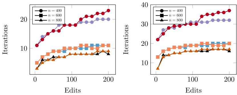
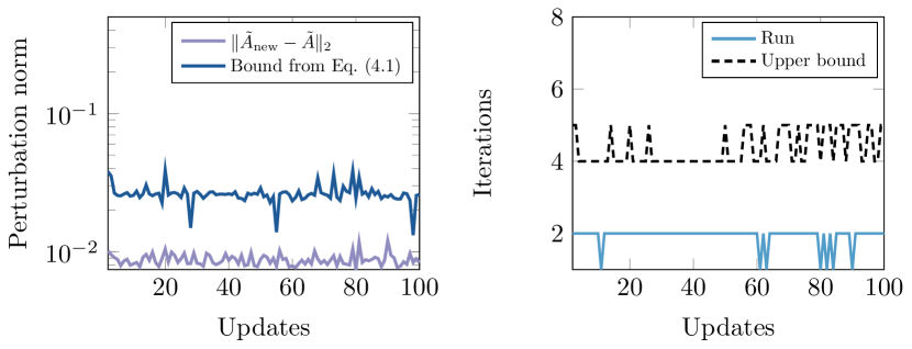
Figure 1: Upper bound from (16) on iterations performed for tracking $V\in\mathbb{R}^{n\times 5}$ using Algorithm 1 without (cold colors) vs. with (warm colors) eigengap oracle. The resulting bounds exhibit negligible differences. Underlying graphs are SBMs with $p=0.5,q=0.1$. Left: $\varepsilon=10^{-2}$. Right: $\varepsilon=10^{-3}$.

Figure 2: Performance of Algorithm 3 for tracking $V\in\mathbb{R}^{n\times 5}$ using the bound from Eq. 20 with $\alpha<0.05$ (left) and resulting iterations (right). The perturbation bound is at most an order of magnitude off, with the resulting iteration bound just a constant multiple of those elapsed to reach accuracy $\varepsilon=10^{-3}$. Underlying graphs are SBMs with $p=0.5,q=0.1,n=1000$.

All instances generated for this experiment interpolate between a graph with five clusters and one with six clusters, so we expect the eigengap $\lambda_{r+1}-\lambda_{r}$ to gradually decrease; therefore the lowest-dimensional example ($n=400$) should be the most challenging, which is empirically verified. Smaller values of $\varepsilon$ also need fewer subspace iterations, as expected. Finally, by comparing the prescribed accuracy $\varepsilon$ with the final distance of the computed estimates, $\mathrm{dist}(V_{(t)},{\hat{{V}}_{({t})}})$, we find that the latter is at least $2$ orders of magnitude smaller, a somewhat unsurprising outcome given the pessimistic nature of most perturbation results used above.

Effect of sparse updates to spectrum

We take a further step to assess the impact of sparse updates via the lens provided by Proposition 4.1. More precisely, we generate an SBM with $n=1000$ nodes and $5$ communities, with $p=0.5$, $q=0.1$ as previously. We then generate a sequence of $100$ random updates, each corresponding to $50$ edge modifications. As clusters are sizeable and the intra-cluster edge probability $p$ is moderately high, each of these updates results in $\alpha<0.05$ in the notation of Proposition 4.1.

The performance of Algorithm 3 using the worst-case estimate of Eq. 20 to majorize the Davis–Kahan bound is illustrated in Fig. 2. The estimate is at most an order of magnitude higher than the true perturbation norm. Moreover, the resulting bound on iterations is off by a constant factor. Therefore, in situations where we observe sparse updates to graphs with few isolated nodes, it is possible to get additional speedups by replacing $d_{t}$ from Eq. 17 with a less complicated proxy.

4.1.2 Time-evolving real-world graphs

We next test our algorithms on real-world graph datasets: the college-msg [46] dataset of private communications on a Facebook-like college messaging platform, as well as subsets of the temporal-reddit-reply dataset [40] consisting of replies between users on the public social media platform reddit.com. All datasets are anonymized and contain timestamped edges representing the interactions. We make edges undirected and remove any duplicates during preprocessing. We isolate the largest connected component and work on the induced subgraph for each dataset, leading to the statistics shown in Table 1. For the reddit-* datasets, small, medium and large variants correspond to keeping the first $N=\left\{100000,250000,1000000\right\}$ nodes of the raw data, respectively.

Table 1: Summary statistics of temporal graphs used in numerical experiments.

Dataset	# of Nodes	# of Edges
college-msg	1,893	13,834
reddit-small	78,529	455,864
reddit-medium	217,286	1,698,265
reddit-large	757,015	5,487,069

As before, we isolate the subgraph $G=(\mathcal{V},\mathcal{E})$ corresponding to the largest connected component of the static version of the graph, and start from a version $G_{s}=(\mathcal{V}_{s},\mathcal{E}_{s})$ such that $\mathcal{V}_{s}=\mathcal{V},\mathcal{E}_{s}\subset\mathcal{E}$, containing the $\left|\mathcal{E}_{s}\right|$ edges with the earliest timestamps. Then, we add edges in the order they were encountered in the original dataset.

We employ a regularized version of the normalized adjacency matrix [2, 30, 51, 70]. Specifically, given a regularization parameter $\tau$, the regularized adjacency matrix is $A_{\tau}:=A+\frac{\tau}{n}\bm{1}\bm{1}^{\top}$. We set $\tau$ equal to $1$ for the college-msg dataset and equal to the average degree ($\tau=\frac{1}{n}\sum_{i=1}^{n}D_{ii}$), for the reddit-* datasets. This regularization can improve spectral clustering by addressing the adverse effects of isolated or low-degree nodes. In particular, the large cluster of the leading eigenvalue (corresponding to connected components in the graph), can significantly degrade the performance of both iterative methods.

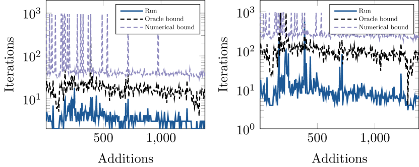
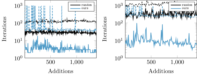
Figure 3: Performance of Algorithm 3 using block Krylov method (left) and subspace iteration (right) on the college-msg dataset, with accuracy $\varepsilon=10^{-3}$. Both plots indicate that the bound of (16) can be sharp, even though it is loose in general.

Figure 4: Iterations using the Davis–Kahan bound and Algorithm 1 (left) vs. Algorithm 2 (right), starting from $V_{0}$ (ours) vs. a random initial estimate (random) on the college-msg dataset ($\varepsilon=10^{-3}$). Solid lines are iterations until numerical convergence, dashed lines are upper bounds. Naive seeding incurs orders of magnitude higher computational costs, which can even exceed the (conservative) upper bound of Eq. 16.

At each step, we use the previous estimate $\hat{V}$ of the leading subspace of $A:=A_{\tau}$ to initialize subspace iteration. Moreover, if we detect a change in the dimension of the invariant subspace (using the criterion in Section 3.2.4), we follow the steps below to form $\hat{V}_{\mathrm{new}}$:

• if $r_{\mathrm{new}}<r$, we simply drop the eigenvectors $v_{i}$ corresponding to the smallest Ritz values $\theta_{i}=\lambda_{i}(\hat{V}^{\top}A\hat{V})$.

• if $r_{\mathrm{new}}>r$, we generate $r_{\mathrm{new}}-r$ new vectors and orthogonalize them against $\hat{V}$ using the (modified) Gram-Schmidt process [22].

Initially, we experiment with the college-msg dataset, as it is feasible to evaluate the true subspace distances and to compare with the performance of the randomly initialized variant at each step. Figure 4 shows the number of iterations run to attain the desired accuracy (checked using numerical stopping criteria) of $\varepsilon=10^{-3}$, as well as the number of iterations $k_{\max}$ determined by Eq. 16, starting from $G_{s}$ and evolving towards the static version of the graph. As in the SBM case, we observe five edge modifications at a time. The plot reveals that our bounds are essentially sharp, since there is more than one occasion where the number of subspace iterations almost matches the upper bound (appearing as spikes).

We also observe that our warm-starting methods provides substantial performance gains compared to random initialization. Figure 4 compares our pipeline with randomly initialized subspace iteration. We set $d_{t}:=\mathrm{dist}(V,\hat{V})$, with $\hat{V}$ being the Q factor from the QR decomposition of a random Gaussian matrix, and report the number of iterations elapsed until achieving accuracy $\varepsilon$ starting from $\hat{V}$ as well as the bounds prescribed by Theorems 2.1 and 2.2 using $\rho:=\frac{\lambda_{r+1}(A)}{\lambda_{r}(A)}$ (computed using Arpack). Our upper bound is usually 1–2 orders of magnitude tighter than the bound using random initialization, while far fewer iterations are needed to reach convergence when initializing $V_{0}$ with the previous estimate.

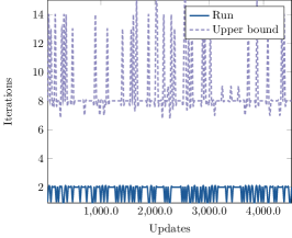
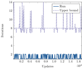
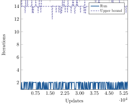
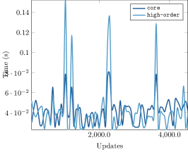
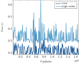
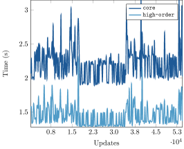
Figure 5: Performance of Algorithm 3 on the reddit-* datasets, using Algorithm 2 as the iterative method. Left to right: small, medium, large with $20$, $25$, and $50$ edge additions per update. Top row: number of iterations per update, which appear to be practically constant and dimension-independent. Bottom row: time elapsed computing $V$ (core) and higher order eigenvalues (high-order); both times are comparable to each other, with the total scaling linearly as $n$ increases.

Next, we evaluate our method on the reddit-* datasets, as depicted in Fig. 5. In this case, Algorithm 2 requires just a handful of iterations per update. Our upper bound is at most an order of magnitude loose and independent of the underlying problem dimension. We are thus able to handle large problems with $\mathcal{O}(1)$ additional iterations per update, in contrast to random initialization which would be expected to scale with dimension.

We also observe that the measured wall-clock times spent updating the subspace $V$ and the higher-order eigenvalues $\left\{\hat{\lambda}_{r+1},\dots\right\}$ are comparable. In fact, the majority of each step is spent on estimating $\left\|E\right\|_{2}$. Importantly, the time elapsed per iteration appears to scale linearly as $n$ increases, which is the expected behavior given the edge density in Table 1 (here, edge density exactly controls the complexity of matrix-vector multiplication).

4.2 Principal Component Analysis

This section evaluates the performance of our adaptive method on Principal Component Analysis (PCA) [29]. In this setting, we have a data matrix $X\in\mathbb{R}^{n\times d}$, containing $n$ points in $d$ dimensions. For a target dimension $p$, we wish to compute $W\in\mathbb{R}^{p\times p}$ so that $W$’s columns are the top-$p$ eigenvectors of $X^{\top}X$. These columns then define a projection $X\mapsto XW\in\mathbb{R}^{n\times p}$ which can be helpful in exploratory data analysis, de-noising, clustering, and other tasks. First, we show how to improve our perturbation bounds under common update models that are applicable to incrementally updated PCA.

4.2.1 Improved bounds under random perturbations

The perturbation bounds for subspaces employed in Algorithm 3 can be greatly simplified when the updates $E_{(t)}$ are random. Below, we consider both general Gaussian random matrices, as well as sums of outer products of Gaussian random vectors. We defer proofs of the technical results below to Appendix B.

Random Gaussian perturbations

Suppose we are given a matrix $A:=A_{(0)}\in\mathbb{R}^{n\times n}$ (we assume $A$ is square for simplicity, but the proof techniques extend to $A\in\mathbb{R}^{m\times n}$). Initially, let us assume that the perturbation matrix is i.i.d. Gaussian, formalized below:

Assumption 3.

For each $t$, the perturbation matrix $E:=E_{(t)}$ satisfies $(E)_{ij}\sim\mathcal{N}\left(0,\frac{1}{n^{2}}\right)$, with all the elements independent of each other.

To derive a priori bounds for the subspace distances, we use the analogue of Davis–Kahan for singular subspaces, due to Wedin [67]. Under 3, we show that the distances between singular subspaces are upper bounded and that the singular values of $A,\tilde{A}$ are only off by a factor of $\tilde{\mathcal{O}}(n^{-1})$. Both statements hold with high probability, leading to Proposition 4.2.

Proposition 4.2.

Let 3 hold and let $A$, $\tilde{A}:=A+E$ have SVDs given by $A=U\Sigma V^{\top},\;\tilde{A}=\tilde{U}\tilde{\Sigma}\tilde{V}^{\top}$. Then, with probability at least $1-c_{1}\exp(-c_{2}n)-2n^{-\frac{\log n}{2}}$,

(22) $$\max\left\{\left\|\sin\Theta(U_{1},\tilde{U}_{1})\right\|,\left\|\sin\Theta(V_{1},\tilde{V}_{1})\right\|\right\} \leq\frac{2/\sqrt{n}+\sqrt{r}/n}{\sigma_{r}-\sigma_{r+1}-(C_{A}+\log n)/n},$$

where $c_{1},c_{2}$ are universal constants and $C_{A}$ is a constant only depending on $A$.

Low-rank random perturbations

In a different setting, we observe updates to the covariance matrix $A=XX^{\top}$ in which the perturbation matrix $E$ is not i.i.d. Gaussian but obeys a low-rank structure, as described below:

Assumption 4.

For each $t$, the random perturbation $E_{(t)}$ satisfies

$$E_{(t)}=\varepsilon_{t}z_{t}z_{t}^{\top},$$

where $z_{t}\sim\mathcal{N}(0,1/n)$ and with $\varepsilon_{t}$ independent of $z_{t}$.

Suppose the above assumption holds and we want to retain information about a $r$-dimensional subspace, $r\ll n$, over time. When we apply the a priori bound from Theorem 3.2, assuming $\delta_{r}>2\left\|E\right\|_{2}$, we are reduced to bounding $\left\|E_{(t)}V_{0}\right\|_{2}$ in the numerator, with $V_{0}\in\mathbb{R}^{n\times r}$. Using standard tools from concentration of measure, we can show the following:

Proposition 4.3.

Let 4 hold (dropping the subscript for simplicity), and suppose that $\delta_{r}>2+\epsilon$. Let $\tilde{A}=A+E$ and let $V,\tilde{V}$ correspond to the leading $r$-dimensional subspaces of $A,\tilde{A}$ respectively. Then, with probability at least $1-\exp\left(-\frac{\epsilon^{2}n}{32}\right)-n^{-1}$,

(23) $$\left\|\sin\Theta(V,\tilde{V})\right\|_{2}\leq\frac{1+\epsilon}{\delta_{r}}\left(\sqrt{\frac{r}{n}}+\sqrt{\frac{2\log n}{n}}\right).$$

This bound can be directly applied for the estimate $d_{t}$ in Algorithm 3.

4.2.2 Synthetic experiments

We perform two experiments on synthetic data, starting from an appropriately scaled Gaussian random matrix $X_{0}\in\mathbb{R}^{n\times d}$, using the two variations of random updates described in Section 4.2.1. For each variation, we apply our adaptive method to keep track of a subspace of dimension at most $\lfloor\sqrt{n}\rfloor$, which is updated using Eq. 19. At each step, we record the true subspace distance as well as the refined a priori bounds derived in the aforementioned sections.

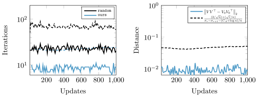
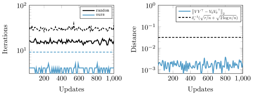
Figure 6: PCA on synthetic data. Top: $(n,d)=(1500,1500)$ following 3. Bottom: $(n,d)=(2000,500)$ following 4. Left: iterations of Algorithm 2 to reach accuracy $\varepsilon=10^{-3}$ (solid) vs. upper bounds (dashed). Right: oracle distance vs. bounds from Propositions 4.3 and 4.2. Updating without warm-starting in practice is more expensive than the worst-case bounds of Algorithm 3 even when the subspace distance estimates are loose.

Figure 6 shows the performance of Algorithm 3. In terms of required iterations, our method clearly outperforms reinitializing with a random matrix. In fact, the upper bound derived from perturbation theory falls below the number of iterations required to reach the desired accuracy starting from a random guess, as in Fig. 4. This means that even the worst-case performance of the warm-starting method can be significantly better than naive seeding in simple examples.

4.2.3 Singular Spectrum Analysis for time series data

An application of PCA is Singular Spectrum Analysis (SSA) [20, 23], which is primarily applied in time series analysis. To apply SSA, one specifies a window length $W$ that is expected to capture the essential behavior of the time series of length $N\geq W$, and performs the following steps (following [23]):

1. Form the trajectory matrix of the series $X$

   $$C_{X}:=\frac{1}{\sqrt{N}}\begin{pmatrix}X_{1}&X_{2}&X_{3}&\dots&X_{N-W+1}\\ X_{2}&X_{3}&X_{4}&\dots&X_{N-W+2}\\ \vdots&&&&\vdots\\ X_{W}&X_{W+1}&X_{W+2}&\dots&X_{N}\end{pmatrix}\in\mathbb{R}^{W\times(N-W+1)}.$$

   Observe that $C_{X}$ is a Hankel matrix, since its antidiagonals are constant, and therefore admits fast matrix-vector multiplication.

2. Compute the truncated SVD $F_{X}$ of $C_{X}$ with target rank $r\ll\min(W,N-W+1)$:

   (24) $$C_{X}\approx F_{X}=\sum_{i=1}^{r}u_{i}\sigma_{i}v_{i}^{\top}.$$

3. Average the antidiagonals of $F_{X}$, from which a smoothed time series can be extracted.

We applied SSA on the Household Power Consumption dataset, available from the UCI Machine Learning Repository. The dataset contains power consumption readings for a single household spanning 4 years, spaced apart by a minute. We preprocess the dataset by computing the moving averages of active power over $30$ minutes with a forward step of $20$ minutes, resulting in $3$ data points per hour. We set the window and series lengths $\left\{W,N\right\}=(4032,12096)$, which correspond to roughly 2 and 6 months of consumption, respectively; this means that $C_{X}$ is the trajectory matrix for the most recent $6$ months.

Next, we applied Algorithm 3 to maintain the decomposition of the trajectory matrix $C_{X}$ over time, with $r$ equal to the value specified by the criterion in Eq. 19. Each update “step” moves the time series forward by $6$ measurements (or $2$ hours). The resulting dimension is determined as $r=4$ in every time step, satisfying $\frac{\left\|\Sigma_{1:r}\right\|_{F}}{\left\|\Sigma\right\|_{F}}\geq 99\%$ throughout.

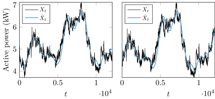
Figure 7: Original ($X_{t}$) and reconstructed ($\hat{X}_{t}$) signals after the equivalent of $15$ (left) and $30$ (right) days of updates, using $r=4$ components and accuracy $\varepsilon=10^{-3}$. The low-rank reconstruction captures the essential behavior of the time series.

Figure 7 depicts the original and reconstructed signals after $15$ and $30$ days, respectively. The reconstructed curve captures the essential behavior of the original time series, having “smoothed” out fluctuations on smaller scales. Moreover, with the exception of the first step, all subsequent computations of the singular subspaces take at most $3$ matrix-vector multiplications per step. On the other hand, naive seeding can take up to $20$ matrix-vector multiplications per step.

5 Discussion

This work has detailed the theoretical and practical aspects of incrementally updating spectral embeddings via careful use of existing information—an oft used methodology, albeit one previously employed heuristically. Concisely, we showed how the straightforward heuristic of warm-starting iterative eigensolvers with previously computed subspaces can dramatically decrease the amount of work required to update low-dimensional embeddings under small changes to the data matrix. This is a broadly applicable scenario, encompassing all manners of time-evolving or sequentially observed data. While we have focused on a few specific applications, there is a wider range of settings that fall into this regime such as spectral ranking methods in network analysis [49] or latent semantic indexing in natural language processing [17].

A key insight, and an advantage of our proposed pipeline, is that worst-case bounds on invariant subspace perturbations can be efficiently computed before updates to the spectral embedding are carried out. This added information can be used both theoretically, to bound the number of “clean-up” iterations that need to be carried out, and practically, to determine if the dimension of the subspace should change. Furthermore, the bounds simplify with additional assumptions on the incremental updates such as sparsity or randomness. Presenting this work in a predominantly algorithm-agnostic manner makes the underlying conclusions applicable to any iterative method that can be warm-started. This broadens the applicability of our analysis and strengthens its implications.

We have focused on the dominant eigenspace, though Algorithm 3 carries over to the complementary setting. However, an added complexity may be the need to repeatedly solve closely related linear systems; the nature of the incremental updates may admit ways to address this concern, and we defer such challenges to future work. Additional challenges pertain to removing 2 on the spectral decay, though we consider it rather nonrestrictive. Nevertheless, in the presence of “challenging” spectra, warm-starting can help reduce the cost per update and still outperform e.g., algebraic methods, especially when matrix-vector multiplication is cheap. Lastly, while we have considered the problem dimension to be fixed throughout, an assumption that may be violated in practice, we believe it is possible to pair this work with careful augmentation of the existing subspace to address that problem.

Appendix A Auxiliary results

A.1 Concentration of measure

Let us recall some results and definitions which are used in later proofs. The following Lemma is very useful for bounding the norm of Gaussian random vectors. It appears as part of Lemma 1 in [34]:

Lemma A.1.

Let $(Y_{1},\dots,Y_{D})$ be standard Gaussian variables. Let $\alpha=(a_{1},\dots,a_{D}),a_{i}\geq 0$ and define $Z:=\sum_{i=1}^{D}a_{i}(Y_{i}^{2}-1)$. Then, $\forall x>0$, we have:

When dealing with Gaussian processes, it is common to encounter the concept of Gaussian width:

Definition A.2.

Let $T\subset\mathbb{R}^{n}$ be a bounded set and $g\sim\mathcal{N}(0,I_{n})$ a standard Gaussian random variable. The Gaussian width of $T$ is defined as

(26) $$\mathcal{W}(T):=\mathbb{E}\left[\sup_{x\in T}\left\langle g,x\right\rangle\right].$$

One of several bounds on the Gaussian width of a set is outlined below. It is a straightforward consequence of [63, Exercise 7.6.1 & Lemma 7.6.3]:

Lemma A.3.

Consider $T\subset\mathbb{R}^{n}$ and let $\mathrm{diam}(T):=\sup_{x\in T}\left\|x\right\|_{2}$ and $\dim(T)$ denote its algebraic dimension. Then

(27) $$\mathcal{W}(T)\leq\mathrm{diam}(T)\sqrt{\dim(T)}$$

Finally, it is known that Lipschitz functions of Gaussian variables concentrate well around their mean. The following Theorem is standard, see e.g. [63, Chapter 5].

Theorem A.4.

Let $f:\mathbb{R}^{n}\to\mathbb{R}$ be an $L$-Lipschitz function, i.e. $\left|f(x)-f(y)\right|\leq L\left\|x-y\right\|$, $\forall x,y\in\mathbb{R}^{n}$. Then, if $X=(X_{1},\dots,X_{n})\sim\mathcal{N}(0,I_{n})$, it holds that

(28)

A.2 Linear Algebra

Theorem A.5 (Wedin’s $\sin$ theorem).

Let $A,\tilde{A}\in\mathbb{R}^{m\times n}$ with SVDs given by $A=U\Sigma V^{\top}$, $\tilde{A}=\tilde{U}\tilde{\Sigma}\tilde{V}^{\top}$, and let $E:=A-\tilde{A}$. Suppose there exist $\alpha,\delta>0$ such that

$$\min_{i\in[r]}\sigma_{i}>\alpha+\delta,\quad\max_{j\in[n-r]}\tilde{\sigma}_{r+j}<\alpha.$$

Denote by $U_{1},\tilde{U}_{1},V_{1},\tilde{V}_{1}$ the left and right singular subspaces corresponding to the top $r$ singular values. Then for any unitarily invariant norm $\left\|\cdot\right\|$,

(29) $$\max\left\{\left\|\sin\Theta(U_{1},\tilde{U}_{1})\right\|,\left\|\sin\Theta(V_{1},\tilde{V}_{1})\right\|\right\}\leq\frac{\max\left\{\left\|EV_{1}\right\|,\left\|E^{\top}U_{1}\right\|\right\}}{\delta}.$$

Theorem A.6 (Theorem 3.6 in [3]).

Consider a Hermitian matrix $A$ and an $A$-invariant subspace $\mathcal{X}$, corresponding to a contiguous set of eigenvalues of $A$. Then, for any other subspace $\mathcal{Y}$ with $\dim(\mathcal{X})=\dim(\mathcal{Y})$, it holds that

$$\max_{i}\left|\lambda_{i}(X^{\top}AX)-\lambda_{i}(Y^{\top}AY)\right|\leq\rho(A)\max_{i}\left\{\sin^{2}\theta_{i}(\mathcal{X},\mathcal{Y})\right\},$$

where $\rho(A)$ is the spectral radius of $A$.

Lemma A.7 (Weyl’s inequality).

Let $A,\widehat{A}\in\mathbb{R}^{n_{1}\times n_{2}}$ with $\widehat{A}=A+E$. Then, for all $k$, we have

$$\left|\sigma_{k}(A)-\sigma_{k}(\widehat{A})\right|\leq\left\|E\right\|_{2}.$$

Lemma A.8.

Let $D=\mathrm{diag}(d_{1},\dots,d_{n})$ and $A\in\mathbb{R}^{n\times n}$ with $A=A^{\top}$. Then it holds that

$$\left\|DAD\right\|_{2}\leq\sqrt{\mathrm{rank}(A)}\left\|D^{2}A\right\|_{2}.$$

Proof A.9.

Notice that we can write

$$\left\|D^{2}A\right\|_{F} =\sup_{V:\left\|V\right\|_{F}=1}\left\langle D^{2}A,V\right\rangle\geq\frac{\mathrm{Tr}\left(AD^{2}AD^{2}\right)}{\left\|D^{2}A\right\|_{F}}=\frac{\mathrm{Tr}\left(DADDAD\right)}{\left\|D^{2}A\right\|_{F}}=\frac{\left\|DAD\right\|_{F}^{2}}{\left\|D^{2}A\right\|_{F}},$$

making use of the cyclic property of the trace throughout. Rearranging shows that $\left\|DAD\right\|_{F}\leq\left\|D^{2}A\right\|_{F}$. From norm equivalence $\left\|A\right\|_{2}\leq\left\|A\right\|_{F}\leq\sqrt{\mathrm{rank}(A)}\left\|A\right\|_{2}$, we have

$$\left\|DAD\right\|_{2} \leq\left\|DAD\right\|_{F}\leq\left\|D^{2}A\right\|_{F}\leq\sqrt{\mathrm{rank}(D^{2}A)}\left\|D^{2}A\right\|_{2},$$

with $\mathrm{rank}(D^{2}A)\leq\mathrm{rank}(A)$, which completes the proof.

A.3 Miscellanea

Lemma A.10.

Consider the set of matrices

$$\mathcal{X}_{r}=\left\{X\in\mathbb{R}^{n_{1}\times n_{2}}\ \middle|\ \mathrm{rank}(X)\leq r,\;\left\|X\right\|_{F}\leq 1\right\}.$$

Then the covering number of $\mathcal{X}_{r}$ with respect to the metric $d(M_{1},M_{2}):=\left\|M_{1}-M_{2}\right\|_{F}$ satisfies

$$\mathcal{N}(\mathcal{X}_{r},d,\varepsilon)\leq\left(\frac{9}{\varepsilon}\right)^{(n_{1}+n_{2}+1)r}.$$

Proof A.11.

Notice that we can decompose all matrices in $\mathcal{X}_{r}$ using the (economic) SVD as $X=U\Sigma V^{\top},\;\left\|\Sigma\right\|_{F}\leq 1,\;\Sigma\in\mathbb{R}^{r\times r},\;U\in\mathbb{O}_{n_{1},r},\;V\in\mathbb{O}_{n_{2},r}.$ Then we can cover the set of admissible singular values with a $\frac{\varepsilon}{3}$-net of vectors in $\mathbb{B}_{r}$, which is of cardinality at most $\left(1+\frac{2}{\varepsilon}\right)^{r}\leq\left(\frac{9}{\varepsilon}\right)^{r}$ (see e.g. [63, Chapter 4]). The remainder of the proof involves covering $\mathbb{O}_{n,r}$ and is identical to [10, Lemma 3.1].

Appendix B Omitted proofs

B.1 Proof of Proposition 4.1

Given $E$, we denote $D^{\prime}:=\mathrm{diag}(\epsilon_{1},\dots,\epsilon_{n})$ where $\epsilon_{i}:=\sum_{j=1}^{n}E_{ij}$. Denoting the updated regularized adjacency matrix by $\tilde{A}_{\mathrm{new}}$, it is immediate that we can write

(30) $$\tilde{A}_{\mathrm{new}}:=(D+D^{\prime})^{-1/2}(A+E)(D+D^{\prime})^{-1/2}.$$

The first step is to get an expression for $(D+D^{\prime})^{-1/2}$. Since both matrices are diagonal, we can write

$$(D+D^{\prime})^{-1} =\mathrm{diag}\left(\left\{d_{i}\left(1+\frac{\epsilon_{i}}{d_{i}}\right)\right\}_{i=1}^{n}\right)^{-1}=\mathrm{diag}\left(\left\{\frac{1}{d_{i}}\cdot\frac{1}{1+\frac{\epsilon_{i}}{d_{i}}}\right\}_{i=1}^{n}\right)$$

(31) $$=\mathrm{diag}\left(\left\{\frac{1}{d_{i}}\left(1-\frac{\frac{\epsilon_{i}}{d_{i}}}{1+\frac{\epsilon_{i}}{d_{i}}}\right)\right\}_{i=1}^{n}\right)=\mathrm{diag}\left(\left\{\frac{1}{d_{i}}\left(1-\frac{\delta_{i}}{1+\delta_{i}}\right)\right\}_{i=1}^{n}\right),$$

(32) $$(D+D^{\prime})^{-1/2} =\mathrm{diag}\left(\left\{\frac{1}{\sqrt{d_{i}}}\sqrt{1-\frac{\delta_{i}}{1+\delta_{i}}}\right\}_{i=1}^{n}\right)$$

where $\delta_{i}:=\frac{\epsilon_{i}}{d_{i}}$ in Eq. 31. Next, we can write $\sqrt{1-\frac{\delta_{i}}{1+\delta_{i}}}=1-z_{i}$, with $z_{i}\in\left[\frac{\delta_{i}}{2(1+\delta_{i})},\frac{\delta_{i}(2+\delta_{i})}{2(1+\delta_{i})^{2}}\right]$, based on the identity $1-\frac{x}{2}-\frac{x^{2}}{2}\leq\sqrt{1-x}\leq 1-\frac{x}{2}$. It then follows that $(D+D^{\prime})^{-1/2}=D^{-1/2}(I-Z)$, $Z:=\mathrm{diag}(z_{1},\dots,z_{n})$. Expanding this in the expression of Eq. 30 gives us

(33) $$\begin{aligned} \tilde{A}_{\mathrm{new}}&=D^{-1/2}(I-Z)(A+E)(I-Z)D^{-1/2}\\ &=D^{-1/2}(A-2AZ+ZAZ)D^{-1/2}+(I-Z)D^{-1/2}ED^{-1/2}(I-Z)\\ &=\tilde{A}+Z\tilde{A}Z-2\tilde{A}Z+(I-Z)D^{-1/2}ED^{-1/2}(I-Z).\end{aligned}$$

Therefore, to bound $\left\|\tilde{A}_{\mathrm{new}}-\tilde{A}\right\|_{2}$, we have to bound three major components:

$$\left\|Z\tilde{A}Z\right\|_{2},\quad\left\|\tilde{A}Z\right\|_{2},\quad\text{and}\quad\left\|D^{-1/2}ED^{-1/2}\right\|_{2}.$$

For the first two terms, since $\lambda_{i}(\tilde{A})\in[-1,1]$ [13], we have that:

(34) $$\left\|\tilde{A}Z\right\|_{2} \leq\left\|Z\right\|_{2}=\max_{j\in[n]}\left|z_{j}\right|\leq\frac{\alpha(1+\alpha)}{2},\quad\left\|Z\tilde{A}Z\right\|_{2}\leq\left(\frac{\alpha(1+\alpha)}{2}\right)^{2},$$

with the bound for $\left|z_{i}\right|$ coming from the fact that

$$\left|\frac{\delta_{i}}{2(1+\delta_{i})}+\frac{\delta_{i}^{2}}{2(1+\delta_{i})^{2}}\right|\leq\frac{\alpha}{2}+\frac{\alpha^{2}}{2},\;\text{ since }\left|\delta_{i}\right|\leq\alpha.$$

For the remaining term, we upper bound $\left\|D^{-1/2}ED^{-1/2}\right\|_{2}\leq\left\|D^{-1/2}\right\|\left\|ED^{-1/2}\right\|_{2}$, and by the Gershgorin Circle Theorem [22] (using the columns of $ED^{-1/2}$) we obtain

(35) $$\begin{aligned} \max_{i}\left|\lambda_{i}(ED^{-1/2})\right|&\leq\max_{j\in[n]}\left|\sum_{k=1,k\neq j}^{n}\frac{E_{kj}}{\sqrt{d_{j}}}\right|\overset{(*)}{=}\max_{j\in[n]}\left|\sum_{k=1}^{n}\frac{E_{jk}}{\sqrt{d_{j}}}\right|\leq\max_{j\in[n]}\frac{1}{\sqrt{d_{j}}}\alpha d_{j}\\ \left\|D^{-1/2}ED^{-1/2}\right\|&\leq\left\|D^{-1/2}\right\|_{2}\max_{j\in[n]}\alpha\sqrt{d_{j}}=\alpha\sqrt{\frac{\max_{i}d_{i}}{\min_{j}d_{j}}}=\alpha\sqrt{\kappa(D)},\end{aligned}$$

where $(*)$ follows since $E_{ii}=0,E^{\top}=E$ and the next inequality follows by our assumptions. From Lemma A.8 (applied with $D:=D^{-1/2}$, $A:=E$) we have

(36) $$\left\|D^{-1/2}ED^{-1/2}\right\|_{2} \leq\sqrt{\mathrm{rank}(E)}\left\|D^{-1}E\right\|_{2}\leq\sqrt{\mathrm{rank}(E)}\max_{i\in[n]}\left|\sum_{j=1}^{n}\frac{E_{ij}}{d_{i}}\right|\leq\sqrt{\mathrm{rank}(E)}\alpha,$$

with the penultimate inequality via Gershgorin’s circles. We deduce that

(37) $$\left\|D^{-1/2}ED^{-1/2}\right\|_{2}\leq\min\left(\sqrt{\kappa(D)},\sqrt{\mathrm{rank}(E)}\right)\alpha.$$

Combining Eqs. 34 and 37 into Eq. 33 we complete the proof (noting that $\left\|I-Z\right\|_{2}^{2}\leq 1+\mathcal{O}(\alpha^{2})$ by submultiplicativity and the definition of $Z$):

(38) $$\left\|\tilde{A}_{\mathrm{new}}-\tilde{A}\right\|_{2}\leq\alpha\cdot\left(1+\alpha+\sqrt{\min\left\{\kappa(D),\mathrm{rank}(E)\right\}}\right)+\left(\frac{\alpha(1+\alpha)}{2}\right)^{2}$$

B.2 Proof of Proposition 4.2

The proof of this proposition is a combination of Lemmas B.1 and B.3. The former controls $\left\|EV_{1}\right\|_{2},\left\|E^{\top}U_{1}\right\|_{2}$, while the latter bounds the difference between the corresponding singular values with high probability.

Lemma B.1.

In the setting of Theorem A.5, under 3, it holds that

(39) $$\max\left\{\left\|EV_{1}\right\|_{2},\left\|E^{\top}U_{1}\right\|_{2}\right\}\leq\frac{2}{\sqrt{n}}+\frac{\sqrt{r}}{n}$$

with probability at least $1-2\exp(-\frac{n}{2})$.

Proof B.2.

$$\left\|EV_{1}\right\|_{2} =\sup_{u,v\in\mathbb{S}^{m-1}\times\mathbb{S}^{n-1}}\left\langle u,EV_{1}v\right\rangle=\sup_{u,v\in\mathbb{S}^{m-1}\times\mathrm{ran}(V_{1})}\left\langle u,Ev\right\rangle$$

Then, appealing to the Gaussian flavor of Chevet’s inequality due to Gordon [24], as we can write $E=\frac{1}{n}G,(G)_{ij}\sim\mathcal{N}(0,1)$, we recover

(40) $$\mathbb{E}\left[\left\|EV_{1}\right\|_{2}\right] \leq\frac{1}{n}\left(\mathcal{W}(\mathbb{S}^{n-1})\sup_{x\in\mathrm{ran}(V_{1})}\left\|x\right\|_{2}+\mathcal{W}(\mathrm{ran}(V_{1}))\sup_{x\in\mathbb{S}^{n-1}}\left\|x\right\|_{2}\right)\leq\frac{1}{\sqrt{n}}+\frac{\sqrt{r}}{n},$$

where the last inequality is an appeal to Lemma A.3 for the second term after noticing $\dim(\mathrm{ran}(V_{1}))=r$ combined with the fact that

$$\mathcal{W}(\mathbb{S}^{n-1})=\mathbb{E}\left[\sup_{v:\left\|v\right\|_{2}=1}\left\langle g,v\right\rangle\right]=\mathbb{E}\left[\left\|g\right\|_{2}\right]\leq\sqrt{n}.$$

An identical argument gives the same result for $\left\|E^{\top}U_{1}\right\|_{2}$.

Now, using the identity $\left|\sup f-\sup g\right|\leq\left|\sup f-g\right|$, denoting $f(X):=\sup_{u,v}\frac{1}{n}\left\langle u,Xv\right\rangle$, we recover

$$\left|f(X)-f(Y)\right| \leq\frac{1}{n}\left|\sup_{u,v}\left\langle u,(X-Y)v\right\rangle\right|\leq\frac{1}{n}\sup_{u,v}\cancel{\left\|u\right\|_{2}}\left\|(X-Y)v\right\|_{F}\leq\frac{1}{n}\left\|X-Y\right\|_{F},$$

where the last two inequalities are derived using the Cauchy-Schwarz inequality. Therefore $f$ is a $(1/n)$-Lipschitz function of Gaussian random variables. Theorem A.4 gives

(41) $$\leq$$

hence setting $t=n^{-1/2}$ in LABEL:eq:chevet-hp gives us the desired high probability bound. The proof for $\left\|E^{\top}U_{1}\right\|_{2}$ is completely analogous, and following with a union bound for the two terms we recover the desired probability.

Lemma B.3.

In the setting of Theorem A.5, under 3, it holds with probability at least $1-2e^{-c_{1}n}-2n^{-\frac{\log n}{2}}$ that

(42) $$\left|\sigma_{i}(\tilde{A})-\sigma_{i}(A)\right| \leq\frac{C_{A}}{n}+\frac{\log n}{n}$$

where $C_{A}$ is a constant depending only on $A$ and $c_{1}$ is an absolute constant.

Proof B.4.

Let us write $A=U\Sigma V^{\top}$ and $\hat{A}:=A+E=\hat{U}\hat{\Sigma}\hat{V}^{\top}$ for the singular value decompositions of the two matrices. For a matrix $M$, write $M_{uv}:=\left\langle u,Mv\right\rangle$ for brevity and observe the following decomposition:

(43) $$\begin{aligned} \sigma_{i}(A+E)-\sigma_{i}(A)&=\hat{A}_{\widehat{u}_{i},\widehat{v}_{i}}-A_{u_{i},v_{i}}=A_{\widehat{u}_{i},\widehat{v}_{i}}+E_{\widehat{u}_{i},\widehat{v}_{i}}-A_{u_{i},v_{i}}-E_{u_{i},v_{i}}+E_{u_{i},v_{i}}\\ &=(E_{\widehat{u}_{i},\widehat{v}_{i}}-E_{u_{i},v_{i}})+E_{u_{i},v_{i}}+\left(A_{\widehat{u}_{i}-u_{i},v_{i}}+A_{u_{i},\widehat{v}_{i}-v_{i}}+A_{\widehat{u}_{i}-u_{i},\widehat{v}_{i}-v_{i}}\right)\\ &=(E_{\widehat{u}_{i},\widehat{v}_{i}}-E_{u_{i},v_{i}})+E_{u_{i},v_{i}}-\sigma_{i}(A)\left[(1-\left\langle\widehat{u}_{i},u_{i}\right\rangle^{2})+(1-\left\langle\widehat{v}_{i},v_{i}\right\rangle^{2})\right]\\ &\quad+A_{\widehat{u}_{i}-u_{i},\widehat{v}_{i}-v_{i}},\end{aligned}$$

with the last equality above following since $Av_{i}=\sum_{j=1}^{n}\sigma_{j}(A)u_{j}v_{j}^{\top}v_{i}=\sigma_{i}(A)u_{i}$. The decomposition above hints towards the objects that we need to control to prove that $\sigma_{i}(\hat{A})-\sigma_{i}(A)$ is small in magnitude. To be precise, let us define the set

(44) $$\mathbf{S}_{\delta}:=\left\{(u,v)\in\mathbb{S}^{n-1}\times\mathbb{S}^{n-1}\ \middle|\ \left\|uv^{\top}-u_{i}v_{i}^{\top}\right\|_{F}^{2}\leq\delta^{2},\;\left\langle u,u_{i}\right\rangle\geq 0,\;\left\langle v,v_{i}\right\rangle\geq 0\right\}$$

and the events below:

(45) $$\begin{aligned} \mathcal{E}_{1}&:=\left\{\left\|E\right\|_{2}^{2}\leq\frac{C_{1}(x)}{n}\right\},\quad\mathcal{E}_{2}:=\left\{\left|E_{u_{i},v_{i}}\right|\leq\frac{C_{2}(x)}{n}\right\},\\ \mathcal{E}_{3}&:=\left\{\sup_{u,v\in\mathbf{S}_{\delta}}\left|E_{u,v}-E_{u_{i},v_{i}}\right|\leq\frac{\delta}{\sqrt{n}}+\frac{\delta C_{3}(x)}{n}\right\},\end{aligned}$$

where $C_{1},C_{2},C_{3}$ only depend on $x$. The set $\mathbf{S}_{\delta}$ contains the unit vectors $(u,v)$ such that $E_{u,v}$ is “close” to $E_{u_{i},v_{i}}$ in terms of $L^{2}$ distance, with the condition $\left\langle u,u_{i}\right\rangle,\left\langle v,v_{i}\right\rangle\geq 0$ verifiable from the variational characterization of singular values. The goal is to control the probability of each of $\mathcal{E}_{i}$ being false.

As a first step, notice that Theorem A.5 implies

(46) $$\left\|u_{i}u_{i}^{\top}-\hat{u}_{i}\hat{u}_{i}^{\top}\right\|_{F}^{2}+\left\|v_{i}v_{i}^{\top}-\hat{v}_{i}\hat{v}_{i}^{\top}\right\|_{F}^{2}\leq\frac{2}{\delta_{\mathrm{Wedin}}^{2}}\left\|E\right\|_{2}^{2}\leq\frac{2}{\left(\alpha-\frac{1}{\sqrt{n}}\right)^{2}}\frac{C}{n}=\frac{c_{1}}{n},$$

assuming that $\alpha>\frac{1}{\sqrt{n}}$, with the last inequality above holding with high probability since $\left\|E\right\|_{2}\asymp\frac{1}{\sqrt{n}}$ from elementary arguments in random matrix theory. Notice that the above in particular is equivalent to

(47) $$2(1-\left\langle u_{i},\hat{u}_{i}\right\rangle)+2(1-\left\langle v_{i},\hat{v}_{i}\right\rangle)\leq\frac{c_{1}}{n},\quad\max\left\{1-\left\langle u_{i},\hat{u}_{i}\right\rangle,1-\left\langle v_{i},\hat{v}_{i}\right\rangle\right\}\leq\frac{c_{1}}{n}$$

since $1-\left\langle u_{i},\hat{u_{i}}\right\rangle\leq 1-\left\langle u_{i},\hat{u}_{i}\right\rangle^{2}$ due to all vectors being unitary and $\left\langle u_{i},\hat{u}_{i}\right\rangle\geq 0$; the same line of reasoning applies to $\left\langle v_{i},\hat{v}_{i}\right\rangle$. Equivalently, the above gives us

(48) $$\left\|u_{i}-\hat{u}_{i}\right\|_{2}^{2}+\left\|v_{i}-\hat{v}_{i}\right\|_{2}^{2}\leq\frac{c_{1}}{n},\quad\max\left\{\left\|u_{i}-\hat{u}_{i}\right\|_{2},\left\|v_{i}-\hat{v}_{i}\right\|_{2}\right\}\leq\frac{c_{2}}{\sqrt{n}}$$

The magnitude of the RHS in Eq. 48 will help us determine the correct range for $\delta$ in $\mathcal{E}_{3}$.

For the remainder, consider the Gaussian process $\left\{nE_{u,v}-nE_{u_{i},v_{i}}\right\}_{(u,v)\in\mathbb{S}^{n-1}\times\mathbb{S}^{n-1}}$. Following arguments from [63, Chapter 7], since $nE$ is equal in distribution to a standard Gaussian matrix, we obtain using the standard $L^{2}$ distance:

(49) $$d((u,v),(u^{\prime},v^{\prime}))^{2}:=\left\|nE_{u,v}-nE_{u^{\prime},v^{\prime}}\right\|^{2}_{L^{2}}=\left\|uv^{\top}-u^{\prime}{v^{\prime}}^{\top}\right\|_{F}^{2}\leq\left\|u-u^{\prime}\right\|_{2}^{2}+\left\|v-v^{\prime}\right\|_{2}^{2},$$

where the inequality follows from [63, Exercise 7.3.2]. We can now define the following quantities, which control most of the terms above:

(50) $$\xi_{\delta}:=\sup_{u,v\in\mathbf{S}_{\delta}}E_{u,v}-E_{u_{i},v_{i}},\quad\tilde{\xi}_{\delta}:=\sup_{u,v\in\mathbf{S}_{\delta}}\left|E_{u,v}-E_{u_{i},v_{i}}\right|.$$

Since $0\in\mathbf{S}_{\delta}$ by setting $(u,v)=(u_{i},v_{i})$, it follows that

$$\sup_{u,v\in\mathbf{S}_{\delta}}E_{u,v}-E_{u_{i},v_{i}},\quad\sup_{u,v\in\mathbf{S}_{\delta}}-(E_{u,v}-E_{u_{i},v_{i}})\geq 0$$

and also that $\left\|\tilde{\xi}_{\delta}\right\|_{\psi_{2}}\asymp\left\|\xi_{\delta}\right\|_{\psi_{2}}$, with $\left\|\cdot\right\|_{\psi_{2}}$ denoting the subgaussian norm. To arrive at the result, we need the following Lemma:

Lemma B.5.

For $\tilde{\xi}_{\delta}$ defined as in Eq. 50, it holds that

$$\left\|\tilde{\xi}_{\delta}\right\|_{\psi_{2}}\lesssim\left(\frac{\delta}{n}\right)^{2},\;\quad\mathbb{E}\left[\tilde{\xi}_{\delta}\right]\lesssim\frac{\delta}{\sqrt{n}}.$$

Proof B.6.

The proof of the first property is immediate since Eq. 49 and the fact that we are working within $\mathbf{S}_{\delta}$ give us

$$\sup_{u,v\in\mathbf{S}_{\delta}}\left\|E_{u,v}-E_{u_{i},v_{i}}\right\|^{2}_{L^{2}}=\sup_{u,v\in\mathbf{S}_{\delta}}\frac{1}{n^{2}}\left\|uv^{\top}-u_{i}v_{i}^{\top}\right\|_{F}^{2}\leq\frac{\delta^{2}}{n^{2}},$$

hence the result for the subgaussian norm follows from the high-probability version of Dudley’s theorem [63, Theorem 8.1.6].

For the latter property, let us write $Z_{u,v}=nE_{u,v}$, so that $Z:=nE$ is a standard Gaussian matrix. Then, using Dudley’s inequality, it follows that

(51) $$\mathbb{E}\left[\xi_{\delta}\right] =\frac{1}{n}\mathbb{E}\left[\sup_{u,v\in\mathbf{S}_{\delta}}Z_{u,v}-Z_{u_{i},v_{i}}\right]\leq\frac{c_{1}}{n}\int_{0}^{\delta}\sqrt{\log\mathcal{N}(\mathbf{S}_{\delta},d,\varepsilon)}\mathrm{d}{\varepsilon},$$

with $\mathcal{N}(\mathcal{S},d,\cdot)$ denoting the covering number of $\mathcal{S}$ with respect to the metric $d$, and the upper limit $\delta$ following since $\mathcal{N}(\mathbf{S}_{\delta},d,\varepsilon)=1,\;\forall\varepsilon>\delta$ as the distance between two “points” indexed by $\mathbf{S}_{\delta}$ is never more than $\delta$.

To estimate $\mathcal{N}(\mathbf{S}_{\delta},d,\varepsilon)$, it suffices to notice that

$$d((u,v),(u_{i},v_{i}))=\left\|uv^{\top}-u_{i}v_{i}^{\top}\right\|_{F}\in\left\{X\in\mathbb{R}^{n\times n}\ \middle|\ \mathrm{rank}(X)\leq 2,\;\left\|X\right\|_{F}\leq\delta\right\},$$

which is just a scaled version of $\mathcal{X}_{2}$ appearing in Lemma A.10. Therefore it must satisfy

$$\mathcal{N}(\mathbf{S}_{\delta},d,\varepsilon)\leq\mathcal{N}(\delta\mathcal{X}_{2},d,\varepsilon)\lesssim\left(\frac{9\delta}{\varepsilon}\right)^{4n+2}.$$

Substituting the above into the integral of Eq. 51, we recover that

$$\mathbb{E}\left[\xi_{\delta}\right]\leq\frac{c_{1}}{n}\int_{0}^{\delta}\sqrt{(4n+2)\log\frac{9\delta}{\varepsilon}}\mathrm{d}{\varepsilon}\asymp\frac{\delta}{\sqrt{n}}.$$

Given Lemma B.5, we can deduce that Moreover, we know that $\left\langle u_{i},Ev_{i}\right\rangle\sim\frac{1}{n}g,\;g\sim\mathcal{N}(0,1)$ and therefore it follows from Gaussian concentration that

Finally, an appeal to [63, Corollary 7.3.3] gives us that

so we can deduce (via a union bound) that , by setting $c:=\max(c_{2},c_{4})$ using the notation above. Then, returning to Eq. 43, we deduce that

$$\left|\sigma_{i}(A+E)-\sigma_{i}(A)\right| \leq 2\frac{\delta}{\sqrt{n}}+\frac{\log n}{n}+\sigma_{i}(A)\frac{C}{n}+\left\|A\right\|_{2}\frac{C^{\prime}}{n}$$

Looking back at Eq. 48, it is immediate that $\delta\lesssim\frac{1}{\sqrt{n}}$, which completes the desired claim.

Putting Lemmas B.1 and B.3 together and appealing to Weyl’s inequality for the singular value gap, we deduce that under 3 the desired inequality must hold with probability at least $1-c_{1}\exp(-c_{2}n)-2n^{-\frac{\log n}{2}}$.

B.3 Proof of Proposition 4.3

The proof consists of two components. In order for Theorem 3.2 to be applicable, we need to ensure that $\left\|E\right\|_{2}<\frac{\delta_{r}}{2}$, so given the lower bound on $\delta_{r}$ it would suffice to prove that $\left\|E\right\|_{2}=\left\|\varepsilon_{t}z_{t}z_{t}^{\top}\right\|_{2}=\left\|z_{t}\right\|^{2}\leq 1+\frac{\epsilon}{2},$ which is a straightforward application of $\chi^{2}$-concentration. The other component consists of showing that $\left\|EV_{0}\right\|_{2}$ is small with high probability, which we tackle by bounding its expectation and using Gaussian concentration to obtain a high probability bound.

Let us take care of the first component; we can write $\left\|z_{t}\right\|_{2}^{2}=\sum_{i=1}^{n}\frac{1}{n}g_{i}^{2},\;g_{i}\sim\mathcal{N}(0,1)$. Then Lemma A.1 with $\alpha=\frac{1}{n}\bm{1}$ tells us that Setting $x=\frac{\epsilon^{2}n}{32}$ when $\epsilon$ is small gives us that $\left\|E\right\|_{2}\leq 1+\frac{\epsilon}{2\sqrt{2}}+\frac{\epsilon^{2}}{32}<1+\frac{\epsilon}{2}$ with probability at least $1-\exp\left(-\frac{\epsilon^{2}n}{32}\right)$.

In order to address the second component, we prove the following Lemma:

Lemma B.7.

Suppose 4 holds. Then, for any $r$-dimensional subspace $V_{0}$, there exist constants $c_{1},c_{2}>0$ such that

Proof B.8.

Denote $E\equiv E^{(t)}$ for brevity. Using the variational characterization of singular values, we know that

$$\left\|EV_{0}\right\|_{2} =\sup_{u\in\mathbb{S}^{n-1},v\in\mathbb{S}^{r-1}}\left\langle u,EV_{0}v\right\rangle=\sup_{u\in\mathbb{S}^{n-1},v\in\mathbb{S}^{r-1}}\varepsilon_{t}\left\langle u,z_{t}z_{t}^{\top}V_{0}v\right\rangle\leq\left\|z_{t}\right\|_{2}\sup_{v\in V_{0}\mathbb{S}^{r-1}}\left\langle z_{t},v\right\rangle.$$

Taking expectations and applying the Cauchy-Schwarz inequality:

$$\mathbb{E}\left[\left\|EV_{0}\right\|_{2}\right] \leq\mathbb{E}\left[\left\|z_{t}\right\|^{2}\right]^{1/2}\mathbb{E}\left[\sup_{v\in V_{0}\mathbb{S}^{r-1}}\left\langle z_{t},v\right\rangle^{2}\right]^{1/2}\leq\left(\frac{1}{n}\mathcal{W}(\mathbb{S}^{n-1}\cap\mathrm{ran}(V_{0}))^{2}\right)^{1/2},$$

where the last inequality follows from the fact that $\mathbb{E}\left[\left\|z_{t}\right\|^{2}\right]=\frac{1}{n}$, the definition of gaussian width, and the fact that $V_{0}$ is an orthogonal matrix, hence $V_{0}$ acting on the unit sphere maps back to the unit sphere. However, $\mathrm{diam}(\mathbb{S}^{n-1}\cap\mathrm{ran}(V_{0}))\leq 1$, and $\dim(T)=\dim(\mathrm{ran}(V_{0}))=r$. An appeal to Lemma A.3 recovers $\mathbb{E}\left[\left\|EV_{0}\right\|_{2}\right]\leq\sqrt{\frac{r}{n}}.$

We can now proceed to show that $\left\|EV_{0}\right\|_{2}$ is small with high probability. Let us denote the events

$$\mathcal{E}_{1}:=\left\{\left\|z_{t}\right\|_{2}\leq c_{1}\right\},\quad\mathcal{E}_{2}:=\left\{\sup_{v\in V_{0}\mathbb{S}^{r-1}}\left\langle z_{t},v\right\rangle\leq\sqrt{\frac{r}{n}}+\sqrt{\frac{2r\log n}{n}}\right\}.$$

For the first event, we know from Lemma A.1 that , where $c_{2}$ depends only on $c_{1}$. Additionally, writing $z_{t}=\frac{1}{\sqrt{n}}g,\;g\sim\mathcal{N}(0,I_{n})$, we see that

$$\left|\sup_{v\in V_{0}\mathbb{S}^{r-1}}\left\langle z_{t},v\right\rangle-\sup_{v\in V_{0}\mathbb{S}^{r-1}}\left\langle z^{\prime}_{t},v\right\rangle\right| \leq\left|\sup_{v\in V_{0}\mathbb{S}^{r-1}}\left\langle z_{t}-z^{\prime}_{t},v\right\rangle\right|\leq\frac{1}{\sqrt{n}}\left\|g-g^{\prime}\right\|,$$

which means that $f(X):=\frac{1}{\sqrt{n}}\sup_{v\in V_{0}\mathbb{S}^{r-1}}\left\langle X,v\right\rangle$ is a $(1/\sqrt{n})$-Lipschitz function of Gaussian variables. Theorem A.4 then implies

$$\leq\exp\left(-\frac{t^{2}}{2L^{2}}\right)$$

$$\Rightarrow \leq\frac{1}{n}.$$

Taking a union bound over $\mathcal{E}_{1}^{c},\mathcal{E}_{2}^{c}$ we recover

Finally, to conclude the proof, we set $c_{1}=1+\frac{\epsilon}{2\sqrt{2}}+\frac{\epsilon^{2}}{32}$ in the definition of $\mathcal{E}_{1}$ above, which gives $c_{2}=\frac{\epsilon^{2}}{32}$.

References

- [1] E. Abbe, J. Fan, K. Wang, and Y. Zhong, Entrywise eigenvector analysis of random matrices with low expected rank, arXiv preprint arXiv:1709.09565, (2017).
- [2] A. A. Amini, A. Chen, P. J. Bickel, and E. Levina, Pseudo-likelihood methods for community detection in large sparse networks, Ann. Statist., 41 (2013), pp. 2097–2122, https://doi.org/10.1214/13-AOS1138.
- [3] M. Argentati, A. Knyazev, C. Paige, and I. Panayotov, Bounds on changes in ritz values for a perturbed invariant subspace of a hermitian matrix, SIAM Journal on Matrix Analysis and Applications, 30 (2008), pp. 548–559, https://doi.org/10.1137/070684628.
- [4] S. Balakrishnama and A. Ganapathiraju, Linear discriminant analysis-a brief tutorial, Institute for Signal and information Processing, 18 (1998), pp. 1–8.
- [5] A. Balsubramani, S. Dasgupta, and Y. Freund, The fast convergence of incremental pca, in Advances in Neural Information Processing Systems, 2013, pp. 3174–3182.
- [6] M. Belkin and P. Niyogi, Laplacian eigenmaps for dimensionality reduction and data representation, Neural computation, 15 (2003), pp. 1373–1396.
- [7] L. Bottou, F. Curtis, and J. Nocedal, Optimization methods for large-scale machine learning, SIAM Review, 60 (2018), pp. 223–311, https://doi.org/10.1137/16M1080173.
- [8] M. Brand, Fast low-rank modifications of the thin singular value decomposition, Linear algebra and its applications, 415 (2006), pp. 20–30.
- [9] J. R. Bunch and C. P. Nielsen, Updating the singular value decomposition, Numerische Mathematik, 31 (1978), pp. 111–129.
- [10] E. J. Candes and Y. Plan, Tight oracle inequalities for low-rank matrix recovery from a minimal number of noisy random measurements, IEEE Transactions on Information Theory, 57 (2011), pp. 2342–2359.
- [11] J. Cape, M. Tang, and C. E. Priebe, The two-to-infinity norm and singular subspace geometry with applications to high-dimensional statistics, arXiv e-prints, (2018), https://arxiv.org/abs/1705.107325.
- [12] Y. Chen, T. A. Davis, W. W. Hager, and S. Rajamanickam, Algorithm 887: Cholmod, supernodal sparse cholesky factorization and update/downdate, ACM Transactions on Mathematical Software (TOMS), 35 (2008), p. 22.
- [13] F. R. K. Chung, Spectral Graph Theory, no. 92 in CBMS Regional Conference Series in Mathematics, American Mathematical Society, 1997.
- [14] J. Cullum and W. E. Donath, A block lanczos algorithm for computing the q algebraically largest eigenvalues and a corresponding eigenspace of large, sparse, real symmetric matrices, in 1974 IEEE Conference on Decision and Control including the 13th Symposium on Adaptive Processes, 1974, pp. 505–509, https://doi.org/10.1109/CDC.1974.270490.
- [15] A. Damle and Y. Sun, Uniform bounds for invariant subspace perturbations, arXiv e-prints, (2019), arXiv:1905.07865, https://arxiv.org/abs/1905.07865.
- [16] C. Davis and W. M. Kahan, The rotation of eigenvectors by a perturbation. III, SIAM Journal on Numerical Analysis, 7 (1970), pp. 1–46.
- [17] S. Deerwester, S. T. Dumais, G. W. Furnas, T. K. Landauer, and R. Harshman, Indexing by latent semantic analysis, Journal of the American Society for Information Science, 41 (1990), pp. 391–407.
- [18] J. W. Demmel, Applied Numerical Linear Algebra, Society for Industrial and Applied Mathematics, 1997.
- [19] J. Eldridge, M. Belkin, and Y. Wang, Unperturbed: spectral analysis beyond davis-kahan, in Proceedings of Algorithmic Learning Theory, F. Janoos, M. Mohri, and K. Sridharan, eds., vol. 83 of Proceedings of Machine Learning Research, PMLR, 2018, pp. 321–358, http://proceedings.mlr.press/v83/eldridge18a.html.
- [20] J. B. Elsner and A. A. Tsonis, Singular Spectrum Analysis: a new tool in time series analysis, Springer Science & Business Media, 2013.
- [21] J. Fan, K. Wang, Y. Zhong, and Z. Zhu, Robust high dimensional factor models with applications to statistical machine learning, arXiv preprint arXiv:1808.03889, (2018).
- [22] G. H. Golub and C. F. Van Loan, Matrix Computations, Johns Hopkins University Press, 4th ed. ed., 2013.
- [23] N. Golyandina and A. Zhigljavsky, Singular Spectrum Analysis for time series, Springer Science & Business Media, 2013.
- [24] Y. Gordon, Some inequalities for gaussian processes and applications, Israel Journal of Mathematics, 50 (1985), pp. 265–289, https://doi.org/10.1007/BF02759761.
- [25] M. Gu, Subspace iteration randomization and singular value problems, SIAM Journal on Scientific Computing, 37 (2015), pp. A1139–A1173.
- [26] M. Gu and S. C. Eisenstat, Efficient algorithms for updating a strong rank-revealing qr factorization, SIAM Journal on Scientific Computing, (1996), https://doi.org/10.1137/0917055.
- [27] N. Halko, P.-G. Martinsson, and J. A. Tropp, Finding structure with randomness: Probabilistic algorithms for constructing approximate matrix decompositions, SIAM review, 53 (2011), pp. 217–288.
- [28] P. W. Holland, K. B. Laskey, and S. Leinhardt, Stochastic blockmodels: First steps, Social networks, 5 (1983), pp. 109–137.
- [29] I. Jolliffe, Principal Component Analysis, Springer, 2nd ed., 2002.
- [30] A. Joseph and B. Yu, Impact of regularization on spectral clustering, The Annals of Statistics, 44 (2016), pp. 1765–1791.
- [31] M. E. Kilmer and E. De Sturler, Recycling subspace information for diffuse optical tomography, SIAM Journal on Scientific Computing, 27 (2006), pp. 2140–2166.
- [32] A. V. Knyazev, Toward the optimal preconditioned eigensolver: Locally optimal block preconditioned conjugate gradient method, SIAM journal on scientific computing, 23 (2001), pp. 517–541.
- [33] R. Kumar, J. Novak, and A. Tomkins, Structure and evolution of online social networks, in Link Mining: Models, Algorithms, and Applications, Springer New York, 2010, pp. 337–357, https://doi.org/10.1007/978-1-4419-6515-8_13.
- [34] B. Laurent and P. Massart, Adaptive estimation of a quadratic functional by model selection, Annals of Statistics, (2000), pp. 1302–1338.
- [35] J. Leskovec, L. A. Adamic, and B. A. Huberman, The dynamics of viral marketing, ACM Transactions on the Web (TWEB), 1 (2007), p. 5.
- [36] J. Leskovec, A. Rajaraman, and J. D. Ullman, Mining of massive datasets, Cambridge university press, 2014.
- [37] H. Li, H. Jiang, R. Barrio, X. Liao, L. Cheng, and F. Su, Incremental manifold learning by spectral embedding methods, Pattern Recognition Letters, 32 (2011), pp. 1447 – 1455, https://doi.org/10.1016/j.patrec.2011.04.004.
- [38] R.-C. Li, Relative perturbation theory: II. eigenspace and singular subspace variations, SIAM Journal on Matrix Analysis and Applications, 20 (1998), pp. 471–492.
- [39] R.-C. Li and L.-H. Zhang, Convergence of the block lanczos method for eigenvalue clusters, Numerische Mathematik, 131 (2015), pp. 83–113, https://doi.org/10.1007/s00211-014-0681-6.
- [40] P. Liu, A. R. Benson, and M. Charikar, Sampling methods for counting temporal motifs, in Proceedings of the Twelfth ACM International Conference on Web Search and Data Mining, WSDM ’19, New York, NY, USA, 2019, ACM, pp. 294–302, http://doi.acm.org/10.1145/3289600.3290988.
- [41] F. McSherry, Spectral partitioning of random graphs, in Proceedings 42nd IEEE Symposium on Foundations of Computer Science, IEEE, 2001, https://doi.org/10.1109/sfcs.2001.959929.
- [42] C. Musco and C. Musco, Randomized block krylov methods for stronger and faster approximate singular value decomposition, in Advances in Neural Information Processing Systems 28, C. Cortes, N. D. Lawrence, D. D. Lee, M. Sugiyama, and R. Garnett, eds., 2015, pp. 1396–1404.
- [43] A. Y. Ng, M. I. Jordan, and Y. Weiss, On spectral clustering: Analysis and an algorithm, in Advances in neural information processing systems, 2002, pp. 849–856.
- [44] H. Ning, W. Xu, Y. Chi, Y. Gong, and T. Huang, Incremental spectral clustering with application to monitoring of evolving blog communities, in Proceedings of the 2007 SIAM International Conference on Data Mining, SIAM, 2007, pp. 261–272.
- [45] A. Özgür, T. Vu, G. Erkan, and D. R. Radev, Identifying gene-disease associations using centrality on a literature mined gene-interaction network, Bioinformatics, 24 (2008), pp. i277–i285.
- [46] P. Panzarasa, T. Opsahl, and K. M. Carley, Patterns and dynamics of users’ behavior and interaction: Network analysis of an online community, Journal of the American Society for Information Science and Technology, 60 (2009), pp. 911–932.
- [47] M. L. Parks, E. De Sturler, G. Mackey, D. D. Johnson, and S. Maiti, Recycling krylov subspaces for sequences of linear systems, SIAM Journal on Scientific Computing, 28 (2006), pp. 1651–1674.
- [48] B. Parlett, The Symmetric Eigenvalue Problem, Classics in Applied Mathematics, Society for Industrial and Applied Mathematics, 1998, https://doi.org/10.1137/1.9781611971163.
- [49] N. Perra and S. Fortunato, Spectral centrality measures in complex networks, Physical Review E, 78 (2008), https://doi.org/10.1103/physreve.78.036107.
- [50] M. A. Porter, J.-P. Onnela, and P. J. Mucha, Communities in networks, Notices of the AMS, 56 (2009), pp. 1082–1097.
- [51] T. Qin and K. Rohe, Regularized spectral clustering under the degree-corrected stochastic blockmodel, in Advances in Neural Information Processing Systems, 2013, pp. 3120–3128.
- [52] T. Reeves, A. Damle, and A. R. Benson, Network interpolation, arXiv e-prints, (2019), https://arxiv.org/abs/1905.01253.
- [53] K. Rohe, S. Chatterjee, and B. Yu, Spectral clustering and the high-dimensional stochastic blockmodel, The Annals of Statistics, 39 (2011), pp. 1878–1915, https://doi.org/10.1214/11-aos887.
- [54] S. T. Roweis and L. K. Saul, Nonlinear dimensionality reduction by locally linear embedding, Science, 290 (2000), pp. 2323–2326.
- [55] A. Ruhe, Implementation aspects of band lanczos algorithms for computation of eigenvalues of large sparse symmetric matrices, Mathematics of Computation, 33 (1979), pp. 680–687.
- [56] Y. Saad, On the rates of convergence of the lanczos and the block-lanczos methods, SIAM Journal on Numerical Analysis, 17 (1980), pp. 687–706, https://doi.org/10.1137/0717059.
- [57] Y. Saad, Numerical Methods for Large Eigenvalue Problems, Society for Industrial and Applied Mathematics, 2011, https://doi.org/10.1137/1.9781611970739.
- [58] P. Salas, L. Giraud, Y. Saad, and S. Moreau, Spectral recycling strategies for the solution of nonlinear eigenproblems in thermoacoustics, Numerical Linear Algebra with Applications, 22 (2015), pp. 1039–1058.
- [59] S. E. Schaeffer, Graph clustering, Computer Science Review, 1 (2007), pp. 27–64, https://doi.org/10.1016/j.cosrev.2007.05.001.
- [60] G. W. Stewart, Accelerating the orthogonal iteration for the eigenvectors of a hermitian matrix, Numerische Mathematik, 13 (1969), pp. 362–376, https://doi.org/10.1007/BF02165413.
- [61] G. W. Stewart and J.-g. Sun, Matrix Perturbation Theory, Academic Press, 1990.
- [62] D. L. Sussman, M. Tang, D. E. Fishkind, and C. E. Priebe, A consistent adjacency spectral embedding for stochastic blockmodel graphs, Journal of the American Statistical Association, 107 (2012), pp. 1119–1128, https://doi.org/10.1080/01621459.2012.699795.
- [63] R. Vershynin, High-dimensional probability: An introduction with applications in data science, vol. 47, Cambridge University Press, 2018.
- [64] B. Viswanath, A. Mislove, M. Cha, and K. P. Gummadi, On the evolution of user interaction in facebook, in Proceedings of the 2nd ACM workshop on Online social networks, ACM Press, 2009, https://doi.org/10.1145/1592665.1592675.
- [65] U. Von Luxburg, A tutorial on spectral clustering, Statistics and computing, 17 (2007), pp. 395–416.
- [66] S. Wang, Z. Zhang, and T. Zhang, Improved Analyses of the Randomized Power Method and Block Lanczos Method, arXiv e-prints, (2015), https://arxiv.org/abs/1508.06429.
- [67] P.-Å. Wedin, Perturbation bounds in connection with singular value decomposition, BIT Numerical Mathematics, 12 (1972), pp. 99–111, https://doi.org/10.1007/BF01932678.
- [68] D. P. Woodruff, Sketching as a tool for numerical linear algebra, Foundations and Trends® in Theoretical Computer Science, 10 (2014), pp. 1–157.
- [69] Q. Yuan, M. Gu, and B. Li, Superlinear convergence of randomized block lanczos algorithm, in 2018 IEEE International Conference on Data Mining (ICDM), IEEE, 2018, pp. 1404–1409.
- [70] Y. Zhang and K. Rohe, Understanding regularized spectral clustering via graph conductance, in Advances in Neural Information Processing Systems, 2018, pp. 10631–10640.