Fluctuations of Lyapunov exponents in homogeneous and isotropic turbulence

Abstract

In the context of the analysis of the chaotic properties of homogeneous and isotropic turbulence, direct numerical simulations are used to study the fluctuations of the finite time Lyapunov exponent (FTLE) and its relation to Reynolds number, lattice size and the choice of the steptime used to compute the Lyapunov exponents. The results show that using the FTLE method produces Lyapunov exponents that are remarkably stable under the variation of the steptime and lattice size. Furthermore, it reaches such stability faster than other characteristic quantities such as energy and dissipation rate. These results remain even if the steptime is made arbitrarily small. A discrepancy is also resolved between previous measurements of the dependence on the Reynolds number of the Lyapunov exponent. The signal produced by different variables in the steady state is analyzed and the self decorrelation time is used to determine the run time needed in the simulations to obtain proper statistics for each variable. Finally, a brief analysis on MHD flows is also presented, which shows that the Lyapunov exponent is still a robust measure in the simulations, although the Lyapunov exponent scaling with Reynolds number is significantly different from that of magnetically neutral hydrodynamic fluids.

I Introduction

It is well-known that turbulence implies chaotic behaviour Ruelle and Takens (1971); Deissler (1986). The description of chaos in turbulent flows has a wide range of applications ranging from geophysical to engineering flows Lorenz (1963); Yoden and Nomura (1993); Masuoka et al. (2003); Musker (1979); Poirel and Price (2001). In particular, the chaotic study of turbulence is strongly associated with the problem of predictability Leith (1971); Leith and Kraichnan (1972); Lorenz (1963); Aurell et al. (1997); Yoden and Nomura (1993). Chaos theory has also been applied to plasmas and astrophysical flows Kurths and Herzel (1986); Grappin et al. (1986); Huang et al. (1994). In the past few decades, there has been an increasing interest in numerically determining the degree of chaos in turbulent flows.

In recent times, high performance computing has made possible to study chaotic properties of 3D flows using direct numerical simulations (DNS) Berera and Ho (2018); Boffetta and Musacchio (2017); Mohan et al. (2017); Ho et al. (2019); Nastac et al. (2017); Mukherjee et al. (2016); Li et al. (2019). This consists in evolving the Navier-Stokes equations (NSE) using no modelling. Almost two decades ago, DNS in 2D flows were used to study predictability Boffetta et al. (1997); Boffetta and Musacchio (2001). Chaotic properties of 3D turbulence have been also studied using approximate models such as EDQNM closure approximation Métais and Lesieur (1986) or shell models Crisanti et al. (1993); Aurell et al. (1997); Yamada and Saiki (2007). All these works have studied chaos and predictability using the Eulerian description of fluids. A different approach commonly found in literature uses the Lagrangian description of turbulent flows to describe chaos de Divitiis (2018); Lapeyre (2002); Biferale et al. (2005a, b).

Whereas the Lagrangian approach deals with dispersion of pairs of fluid particles, the Eulerian approach measures the evolution of two different flows with similar initial conditions. The study of Lagrangian chaos is widely applied in geophysical Yoden and Nomura (1993); Vannitsem (2017); Guo et al. (2016); Garaboa-Paz et al. (2017); d’Ovidio et al. (2004); Haller and Sapsis (2011); Haller (2015); Abraham and Bowen (2002); Garaboa-Paz et al. (2017) and astrophysical applications Chian et al. (2019); Rempel et al. (2016); Chian et al. (2014) as well as the study of engineering flows Tang et al. (2012); Pedersen et al. (1996) and plasmas Padberg et al. (2007); Falessi et al. (2015); Misguich et al. (1987). In these contexts, chaos is used to characterize mixing and transport properties as well as determining Lagrangian coherent structures (LCS) Shadden et al. (2005). Unlike Eulerian chaos, several statistical analyses of Lagrangian chaos have been done in the past Lapeyre (2002); de Divitiis (2018); Johnson and Meneveau (2015).

Eulerian chaos measures the evolution in state space of two initially close realizations of the velocity field $\bm{u}\equiv\bm{u}\left(\bm{x},t\right)$ and $\bm{u}+\delta\bm{u}$, where $\delta\bm{u}$ is infinitesimal. Given the chaotic nature, the difference between both realizations grows exponentially. This can be expressed as

$$\lvert\delta\bm{u}\left(t\right)\rvert\sim\lvert\delta\bm{u}\left(0\right)\rvert\exp\left(\lambda t\right)\quad.$$ (1)

Here $\lambda$ is the maximal Lyapunov exponent. This exponent is a measure of the level of chaos in a turbulent flow Shimada and Nagashima (1979). In other words, it sets the timescale in which the evolution of the flow can be predicted.

Lagrangian chaos statistics have been widely studied compared to the Eulerian case. For the Eulerian case, the method used in Boffetta and Musacchio (2017); Mohan et al. (2017) produces several chaotic realizations that produces different Lyapunov exponents as the flow evolves, this allows to perform a statistical study of Lyapunov exponents. In Mohan et al. (2017), it is noted that the time evolution of such Lyapunov exponent suffers large and fast fluctuations which differ from the fluctuations usually observed in other quantities such as energy or Reynolds number. Hence, a deeper study of the fluctuations of the Lyapunov exponents and their statistical properties is needed. Within a turbulent system there can be two types of fluctuations. One is of stochastic nature, it occurs due to the interaction with noisy environments such as molecular collisions in the small scale. The second type is given by the chaotic nature of the evolution in the NSE due to the non-linear term. These are called deterministic fluctuations. In this work we focus on describing deterministic fluctuations. Unlike experiments, numerical simulation do not introduce unwanted stochastic effects unless deliberately implemented. Thus, in this work, every fluctuation is deterministic.

There are a couple of reasons why we study the fluctuations in the Lyapunov exponents in the Eulerian description of a turbulent flow. One is the magnitude and timescales of such fluctuations are significantly different from other characteristic quantities such as energy, Reynolds number and dissipation. This shows the need to understand the properties of the flow that are particular to chaos and their relation to other parameters in the flow. The other is characterizing the distributions of flow quantities such as Reynolds number, dissipation rate or Lyapunov exponent is the key in any statistical description of turbulence. Applications may be possible since the stability of any quantity may be useful to characterize or calibrate systems.

In 1979, Ruelle predicted that this exponent should be proportional to the inverse of the smallest timescale in the system, that is the Kolmogorov time $\tau=\left(\nu/\varepsilon\right)^{1/2}$, where $\varepsilon$ is the dissipation rate and $\nu$ the kinematic viscosity Ruelle (1979). Ruelle’s prediction uses simple arguments based on dimensional analysis. First, Ruelle states that the maximal Lyapunov exponent should be associated with the smallest timescale of the system, $\tau$. Subsequent work related $\lambda$ to the Reynolds number, $\text{Re}=UL/\nu$, where $U$ is the rms velocity and $L$ the integral length scale. Here $L=(3\pi/2E)\int E(k)/k\ dk$, $E$ being the turbulent kinetic energy and $E(k)$ the energy spectrum. Using Kolmogorov (K41) theory Kolmogorov (1991), it can be deduced that $\lambda\propto(1/T_{0})\text{Re}^{1/2}$, where $T_{0}=L/U$ is the large eddy turnover time.

The relation $\lambda\sim 1/\tau$ proposed by Ruelle is based on very simple considerations. Nevertheless, in practice it is observed that the product $\lambda\tau$ is not constant, but it tends to increase slightly with Reynolds number Boffetta and Musacchio (2017); Berera and Ho (2018). Using a multifractal model, and considering intermittency, the following scaling relation is derived Crisanti et al. (1993)

$$\lambda=\frac{D}{T_{0}}Re^{\alpha}\quad,$$ (2)

where $\alpha=(1-h)/(1+h)$, and $h$ is the Hölder exponent obtained from the structure function $\langle\lvert\bm{u}\left(\bm{x}+\bm{r}\right)-\bm{u}\left(\bm{x}\right)\rvert\rangle\sim Vl^{h}$, where $l=r/L$. In Kolmogorov theory, $h=1/3$ so $\alpha=1/2$ and Ruelle’s scaling is recovered. Using a multifractal model of turbulence Crisanti et al. (1993), the theory predicts a value of $\alpha<0.5$, whereas numerical results show values of $\alpha>0.5$ Boffetta and Musacchio (2017); Berera and Ho (2018).

The paper is organized as follows. In section II, we describe the numerical method used in the simulations as well as the method used to compute the finite time Lyapunov exponents (FTLEs) and flow parameters. In section III, we analyze the distributions obtained for Reynolds number and FTLEs (III.1). Then we look at the relation of the Lyapunov exponent and its fluctuations to lattice size (III.2), Reynolds number (III.3), and the steptime in the FTLE method (III.5). This analysis is done for a hydrodynamic flow evolved using the incompressible NSE . A discrepancy is noted between previous measurements by different authors Boffetta and Musacchio (2017); Berera and Ho (2018). This is resolved by considering corrections given by the dimensionless dissipation rate Mccomb et al. (2015) (III.4). Also for the case of NSE, we perform further analysis for chaos in decaying turbulence. This helps to determine which is the proper timescale to use in the study of Eulerian chaos (III.6).

In section IV, we analyze the timescales in HIT. This is motivated by the fact that Lyapunov exponent signal presents a faster timescale than those of energy and dissipation rate. We make comparisons between different quantities such as energy, dissipation rate and Lyapunov exponents by looking at the decorrelation time in their signals. As a result, we give a useful rule to determine the run time needed to obtain useful statistics from knowledge of the decorrelation time in their signals. It is important to note that even though the analysis is motivated by the study of chaotic properties, it is not restricted to that case only but it is useful in any study of turbulence.

Our main finding is that the Eulerian maximum Lyapunov exponent is a robust measure of the level of chaos in a turbulent flow and gives stable statistics faster than other measurable quantities such as the Reynolds number or energy. Noting that relations like Ruelle’s relate the Lyapunov exponent to other flow parameters such as the Reynolds number, we expect that this finding can be useful to characterize or test systems using the Lyapunov exponents Nastac et al. (2017). Furthermore, we find that the measurements of FTLEs are stable even for very short steptimes, thus reducing the computational cost needed to obtain large sets and improve the statistics.

In section V, a brief analysis is done for Eulerian chaos in an incompressible MHD flow. We observe the distributions of Reynolds number and Lyapunov exponent, and we test the Ruelle’s relation as well as the dependence of the FTLEs on the steptime in the FTLE method. We find that even though Ruelle’s relation does not hold quantitatively for MHD, the Lyapunov exponent is still a robust measure that gives stable statistics faster than other quantities. Finally, in section VI, we discuss the ideas developed across the different sections and we present conclusions.

II Method

In this work, several simulations evolving homogeneous and isotropic flows (HIT) were run using a pseudospectral method and a fully-dealiased DNS code in a periodic box with $N^{3}=32^{3},64^{3},128^{3},256^{3}$ and $512^{3}$ collocation points. Each flow is evolved using the incompressible NSE,

$$\partial_{t}\bm{u}=-\left(\bm{u}\cdot\nabla\right)\bm{u}+\nu\nabla^{2}\bm{u}+\bm{f}\ ,$$ (3)

$$\nabla\cdot\bm{u}=0\quad,$$ (4)

where $\bm{u}\left(\bm{x},t\right)$ is the velocity field and $\bm{f}$ represents an external force per unit volume. A negative damping forcing scheme is implemented. It consists in using the lowest modes in the velocity field $\hat{\bm{u}}\left(\bm{k},t\right)$ (the Fourier transform of $\bm{u}\left(\bm{x},t\right)$) as a forcing function,

$$\hat{\bm{f}}(\bm{k},t)=\begin{cases}\frac{\varepsilon}{2E_{f}}\,\hat{\bm{u}}(\bm{k},t)\quad&\text{if}\quad 0<\lvert\bm{k}\rvert\leq k_{f}\,,\\ 0\quad&\text{otherwise}\quad,\par\end{cases}$$ (5)

where $E_{f}$ is the energy of the velocity field contained in the forcing bandwidth. This well tested forcing function Machiels (1997); Ishihara and Kaneda (2003) has the advantage that the dissipation rate $\varepsilon$ is a parameter that can be set a priori in each simulation. In this case, $\varepsilon$ is set to $0.1$ for all simulations and $k_{f}=2.5$, so only the large scales are forced. The field is initialized with a Gaussian distribution for components of the velocity field including a random seed. A full description of the code and the forcing can be found in Yoffe (2013).

Once the fluid evolution reaches a statistically steady state, the averages of $L,T_{0},U,\varepsilon$ and the finite time Lyapunov exponent $\lambda$ are computed over multiple large eddy turnovers. However, a certain level of fluctuation is always observed. This is possibly associated with the forcing mechanism together with the irregular spatio-temporal behaviour given by the highly non-equilibrium nature of the turbulent regime. A complete understanding and characterizations of these fluctuations are not the aim of this work, but it would be an interesting step to take in the future. Instead, the main goal of this study is to understand the relations between these variables and also with other simulation parameters such as the lattice size $N$. The finite time Lyapunov exponents are computed for each simulation using the method described in the following section.

As well as looking at the evolution of the NSE, we perform a similar analysis for the case of homogeneous and isotropic MHD flows. This analysis consists in evolving the velocity field $\bm{u}$ and the magnetic field $\bm{b}$ using the following incompressible MHD equations

$$\partial_{t}\bm{u} =-\left(\bm{u}\cdot\nabla\right)\bm{u}+\nu\nabla^{2}\bm{u}+\left(\nabla\times\bm{b}\right)\times\bm{b}+\bm{f},$$ (6)

$$\partial_{t}\bm{b} =\left(\bm{b}\cdot\nabla\right)\bm{u}-\left(\bm{u}\cdot\nabla\right)\bm{b}+\eta\nabla^{2}\bm{b}\quad,$$ (7)

together with the incompressibility condition given by Eq.(4) and

$$\nabla\cdot\bm{b}=0\quad,$$ (8)

where $\eta$ is the magnetic diffusion coefficient. For MHD, the Lyapunov exponents measure the divergence of a combination of both the velocity and magnetic fields as described in the following section.

II.1 Finite Time Lyapunov Exponents method

Finite time Lyapunov exponents are widely studied in many applications within the Lagrangian description Yoden and Nomura (1993); Lapeyre (2002); de Divitiis (2018); Shadden et al. (2005); Brunton and Rowley (2010). According to the theory, the Maximal Lyapunov exponent do not depend on the initial infinitesimal perturbation Oseledets (1968), but a slight dependence is usually present for finite perturbations in finite times Goldhirsch et al. (1987). Hence, the Maximal Lyapunov exponent is estimated by averaging over an ensemble of different realizations of finite perturbations in finite times.

In this section, we present the method used in this work to compute the FTLE, which is also used in Boffetta and Musacchio (2017). In the Eulerian description, the procedure used to measure Lyapunov exponents consists in evolving two fields that are initially similar. Given the original field $\bm{u}_{1}$, another field $\bm{u}_{2}=\bm{u}_{1}+\delta\bm{u}$ is created. Then, we evolve the system over a finite steptime $\Delta t$, measure the field difference, and then introduce a successive perturbation, starting the process again each time. The field difference is defined as

$$\delta_{t} =\sqrt{2E_{ud}(t)}\quad,$$ (9)

$$E_{ud} =\frac{1}{2}\int d\bm{k}\lvert\hat{\bm{u}}_{1}\left(\bm{k},t\right)-\hat{\bm{u}}_{2}\left(\bm{k},t\right)\rvert^{2}\,.$$ (10)

The perturbation introduced every steptime $\Delta t$ is given by

$$\bm{u}_{2}(\bm{x},\Delta t)=\bm{u}_{1}(\bm{x},\Delta t)+\frac{\delta_{0}}{\delta_{\Delta t}}\,\delta\bm{u}\left(\bm{x},\Delta t\right)\,,$$ (11)

where $\delta_{0}$ is set to $10^{-3}$ and $\Delta t=0.1$ except in Section III.5.

Each exponent $\tilde{\lambda}$ is measured as

$$\tilde{\lambda}=\frac{1}{\Delta t}\ln\left(\frac{\delta_{\Delta t}}{\delta_{0}}\right)\quad,$$ (12)

and this procedure is repeated, obtaining a set of values for $\tilde{\lambda}$. The mean Lyapunov exponent and its variance were calculated in the usual way

$$\lambda =\langle\tilde{\lambda}\rangle\,,$$ (13)

$$\sigma_{\lambda}^{2} =\frac{1}{n}\sum\langle\tilde{\lambda}^{2}\rangle-\langle\tilde{\lambda}\rangle^{2}\,,$$ (14)

where $n$ is the number of FTLEs measured.

In the case of MHD, we use the same procedure. The only difference is that $\delta_{t}$ is taken as a combination of the increase in both the velocity and magnetic field difference

$$\delta_{t}=\sqrt{2E_{ud}(t)+2E_{bd}(t)}\quad,$$ (15)

where

$$E_{bd}=\frac{1}{2}\int d\bm{k}\lvert\hat{\bm{b}}_{1}\left(\bm{k},t\right)-\hat{\bm{b}}_{2}\left(\bm{k},t\right)\rvert^{2}.$$ (16)

The advantage of the FTLE method is that it produces a sample of Lyapunov exponents that allows us to perform a statistical analysis of the measurements. Other methods exist in literature, for instance, the direct method consists in introducing a small perturbation once the system reaches a steady state and then letting the two fields evolve until they become uncorrelated Berera and Ho (2018); Ho et al. (2019). This method reveals interesting features because it displays the long time evolution of the spectrum of the field difference $\lvert\delta\bm{u}\rvert$ (in which a transient and a saturation stage are found Berera and Ho (2018)). However, this procedure takes a relatively large computational time to get just one Lyapunov exponent. In contrast, the FTLE method is useful to obtain a large number of Lyapunov exponents which can be used to analyze the statistical distribution for a given steady state. This procedure shows that fluctuations in the Lyapunov exponents are quite significant and this fact was not previously noted using the direct method. Hence, it is interesting to analyze the source of such fluctuations and see if they can be explained by other fluctuating quantities in the system.

III Hydrodynamic Results

The values of $\lambda$ measured using the FTLE method produces a time signal with large fluctuations. These fluctuations are briefly mentioned in Boffetta and Musacchio (2017) and some aspects are studied in Mohan et al. (2017); Nastac et al. (2017). In our work, we further analyze the properties of these signals. We look at the mean and standard deviation of $\lambda$ and study their dependence with different flow parameters to see if these variations are of physical origin or if they are caused by the choice of parameters in the numerical simulations.

First, we look at the probability distributions of Re and the FTLEs. Second, we look at how the fluctuations in $\lambda$ depend on the lattice size and Reynolds number. Third, we find a resolution to the discrepancy in results between those of Berera and Ho (2018) which quoted $\alpha=0.53\pm 0.03$ and Boffetta and Musacchio (2017), which had a higher value of $\alpha=0.64\pm 0.05$. Fourth, we observe how the Lyapunov exponent fluctuations depend on the choice of the steptime parameter $\Delta t$ of the FTLE method. Fifth, we study the chaotic behaviour of decaying turbulence and use the high sensitivity of the system with respect to the Lyapunov exponent to test which is the proper large timescale to describe Eulerian chaos.

III.1 Distributions of $\lambda$ and Re

When the fluid reaches a steady state, its statistical quantities such as Re and total energy, fluctuate around a mean value. We first measure the fluctuations in Re, and then observe if these are consistent with the fluctuations measured for $\lambda$.

In Figure 1 we show the typical distributions obtained for Re in the steady state, measured for roughly 10-20 large eddy turnover times. In Figure 2 we show the typical distributions obtained for $\tilde{\lambda}$ in the steady state, measured for the same run time as the equivalent distribution for the Reynolds number.

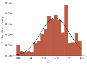
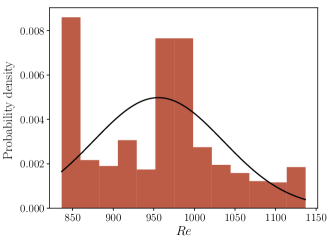
Figure 1: Normalized distributions of Re for three simulations: (a) $N=128$ and $\nu=0.01$ , (b) $N=256$ and $\nu=0.0018$, (c) $N=512$ and $\nu=0.0008$. The black line represents the Gaussian function with mean and variance given by the distribution.

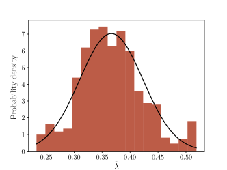
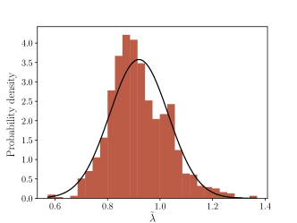
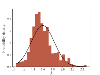
Figure 2: Normalized distributions of $\tilde{\lambda}$ for three simulations: (a) $N=128$ and $\nu=0.01$, (b) $N=256$ and $\nu=0.0018$, (c) $N=512$ and $\nu=0.0008$. The black line represents the Gaussian function with mean and variance given by the distribution.

Surprisingly, most of the distributions of FTLEs are well approximated by a Gaussian whereas the Reynolds numbers histograms were poorly approximated by a Gaussian distribution and even far from a bell shaped distribution in most cases. For a much longer measurement time, the distributions for Re and other large scale statistics approximate a Gaussian distribution more than those in Figure 1. The distribution of Figure 3 shows the distribution for a single run with a measurement time of approximately 500 large eddy turnover times, which corroborated that a Gaussian distribution is approximated for longer run times. However, even after 10-20 large eddy turnover times, the Re statistics approximate a Gaussian very poorly.

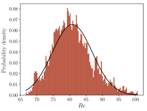
Figure 3: Histogram for the distribution of Re in a single run with measurement time of approximately $500\,T_{0}$. The solid black line represents the Gaussian function with mean and variance corresponding to the data sample

This result may be due to the fact that successive values of Re in a simulation are not random but strongly correlated, whereas for the Lyapunov exponent the correlation is weaker.

It is remarkable that given Equation (2), the distribution of Lyapunov exponents approximates to a Gaussian form when the Reynolds numbers does not even come close to this. Apparently some source of randomization is introduced into the measurement, which could well be a consequence of the perturbation method, which occurs at a relatively high rate. This is one of the most important observations in this paper.

In Figure 4, we present the distribution of $\lambda$ for a simulation with a run time of $200\,T_{0}$, obtaining $n=11863$ values for $\tilde{\lambda}$. From this Figure, we can see that, even though FTLE distributions approximate to a Gaussian, it does not tend to an exact normal distribution for large $n$ and some noise is still observed. The distribution in this Figure has skewness -0.12 and flatness 2.66, where skewness is the third standardized moment of the probability distribution and flatness is the fourth standardized moment. For a Gaussian distribution we would expect skewness to be 0 and flatness to be 3. However, for this simulation, the skewness of total energy, Re, and dissipation is always positive and in the range 0.42-0.46. Flatness is slightly above 3 for these statistics.

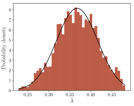
Figure 4: Histogram for the distribution of $\tilde{\lambda}$ in a single run with $N=128$ and $\nu=0.01$, obtaining a large sample of $n=11863$. The solid black line represents the Gaussian function with variance and mean given by the numerical data.

We may measure the FTLE immediately after initializing the simulation, or wait until after the system reaches a statistically steady state. If the FTLE is measured immediately after initialization, there is a initial transient until it reaches a statistically steady state, but this transient is shorter than for the other large scale statistics such as total energy and Reynolds number. This is also provides evidence that the correlation timescale for the Lyapunov exponent is much shorter than for Reynolds number, energy and dissipation rate.

III.2 Dependence of $\lambda$ and Re on lattice size

We look at the dependence of the Lyapunov exponent $\lambda$ and its fluctuations $\sigma_{\lambda}$ on the lattice size. The Lyapunov exponent, Reynolds number and their fluctuations are measured for different runs keeping viscosity and dissipation rate fixed ($\nu=0.01$ and $\varepsilon\sim 0.1$), only varying the lattice size (i.e. $N=32,64,128,256,512$) and random seed for the initial random field. It is important to mention that for each simulation, the mean Reynolds Number obtained are not always the same, ranging between $\sim 75-90$.

In Figure 5, we show the dependence of $\lambda$ on lattice size N for different initial seeds. As can be seen, the Figure shows no correlation or dependence of $\lambda$ on lattice size. The mean values $\lambda$ varies little with $N$ compared to the fluctuations represented in the error bars. In Figure 6, we show the dependence of the fluctuations of the Lyapunov exponent $\sigma_{\lambda}$ on the lattice size. A slight trend is observed in the Figure, although the variation is not significant compared to that given by the variation in Re in the following section and the uncertainty in the value of $\sigma_{\lambda}$ is not relevant given that this affects only the second significant figure in every measurement we perform.

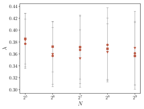
Figure 5: Dependence of $\lambda$ on lattice size $N$, different shapes represent different initial seeds.

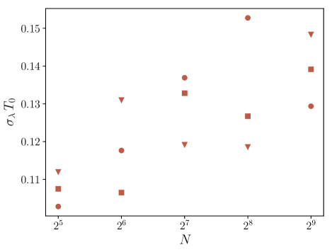
Figure 6: Dependence of Lyapunov exponent fluctuations $\sigma_{\lambda}T_{0}$ vs. $N$, different shapes represent different seeds for the initial random field for each lattice size

III.3 Dependence of $\lambda$ on Re

After determining the variation of the fluctuations with the lattice size, we observe how $\lambda$ and its fluctuations vary depending on the Reynolds number. For this, eleven simulations were run varying viscosity in order to obtain different values of Re ranging between 80 and 1200. Table 1 shows parameter values for all simulations. Once the values for $\lambda,\sigma_{\lambda}$,Re and $\sigma_{\text{Re}}$ are obtained, a weighed least squared fit is performed as shown in Figure 7 to Equation (2), obtaining a value for $\alpha=0.53\pm 0.02$ and $D=0.079\pm 0.007$. These results are in agreement with those previously found in Berera and Ho (2018) in which the same forcing scheme is used but instead of FTLE, the direct method is used.

$N^{3}$	$\nu$	$\varepsilon$	Re	$\lambda$	$\sigma_{\lambda}$	$T_{0}$	$T_{E0}$	$\tau$	$k_{\text{max}}\eta$
$128^{3}$	0.0100	0.096	80.0	0.359	0.057	2.43	5.17	0.323	2.39
$128^{3}$	0.0080	0.097	96.0	0.396	0.057	2.29	5.15	0.287	2.01
$128^{3}$	0.0060	0.097	128.0	0.445	0.064	2.20	5.43	0.249	1.62
$128^{3}$	0.0040	0.101	185.0	0.573	0.099	2.03	5.39	0.199	1.18
$256^{3}$	0.0020	0.098	393.0	0.871	0.153	2.04	5.89	0.143	1.44
$256^{3}$	0.0018	0.099	397.0	0.899	0.123	1.93	5.60	0.135	1.32
$256^{3}$	0.0016	0.098	482.0	0.991	0.194	2.00	5.90	0.128	1.21
$256^{3}$	0.0014	0.099	558.0	1.096	0.256	1.98	5.97	0.119	1.10
$512^{3}$	0.0010	0.100	721.0	1.357	0.218	1.91	5.66	0.100	1.70
$512^{3}$	0.0008	0.099	971.0	1.582	0.270	1.96	5.97	0.090	1.44
$512^{3}$	0.0006	0.100	1174.0	1.877	0.367	1.86	5.67	0.077	1.16

Table 1: Simulation parameters for 11 simulations using incompressible NSE. N is the lattice size, $\nu$ is the kinematic viscosity, $\epsilon$ is the dissipation rate, Re is the Reynolds number, $\lambda$ is the maximal Lyapunov exponent and $\sigma_{\lambda}$ its standard deviation, $T_{0}=L/U$ and $T_{E0}=E/\varepsilon$ are two different definitions for the large eddy turnover time, $\tau$ is the Kolmogorov microscale time, $k_{\text{max}}\approx N/3-1$ is the maximum resolved wavenumber, $\eta=(\nu^{3}/\varepsilon)^{1/4}$ is the Kolmogorov microscale length and $k_{\text{max}}\eta$ is the resolution.

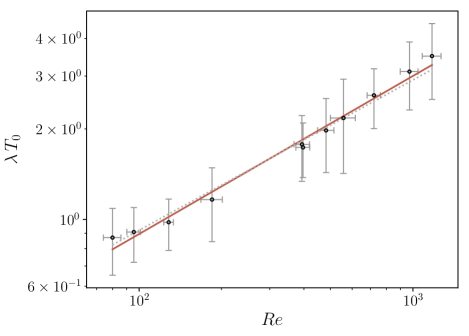
Figure 7: (Color online) $\lambda T_{0}$ vs. Re obtained for eleven simulations where $T_{0}=L/U$. The linear fit is represented by a solid gray (red) line and Ruelle’s prediction is represented by the dotted gray line.

The novel analysis here is done on the fluctuations (deterministic fluctuations as discussed in the Introduction). First, the fluctuations in Re, $T_{0}$ and $\lambda$ are studied. Then, using the relation in Eq.(2), the fluctuations of the quantities on the r.h.s are propagated to estimate the expected level of fluctuations of the Lyapunov exponent on the l.h.s, thus corroborating if the level of fluctuations is consistent on both sides. It is observed that the level of fluctuations in $\lambda$ is larger than that expected from Eq.(2). This might indicate that there are other effects on the system introducing these variations, although it is important to recall that Eq.(2) is not to be taken as a fundamental relation, since it is derived from dimensional considerations. According to the theory, FTLEs have some dependence on the initial finite perturbation and the finite time in which it is measured, so the fluctuations can have origin not only in the fluctuations of the steady state but also by the successive perturbations introduced by the FTLE method and the steptime $\Delta t$.

Figure 8 plots the fluctuations in Re, $\sigma_{\text{Re}}$, against their mean values. It shows that there is a linear dependence in the observed range of Re. The following relation is found, $\sigma_{\text{Re}}=c_{1}\text{Re}$, with $c_{1}=0.08\pm 0.01$. Similarly for the relation between $\lambda$ and $\sigma_{\lambda}$, a linear dependence is observed and the following relation is measured, $\sigma_{\lambda}=c_{2}\lambda$, with $c_{2}=0.20\pm 0.02$. In our simulations, the values for $T_{0}$ and $\sigma_{T_{0}}$ are approximately constant, with $\sigma_{T_{0}}/T_{0}\sim 0.05$.

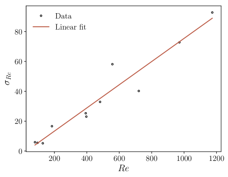
Figure 8: $\sigma_{\text{Re}}$ vs. Re for statistically steady state of the flow and linear fit for slope $c_{1}=0.08\pm 0.01$

To corroborate that these fluctuations are not consistent with Equation (2), we propagate $\sigma_{T_{0}}$ and $\sigma_{\text{Re}}$ and using the measured values we compare the result to the $\sigma_{\lambda}$ obtained using the FTLE procedure. All fluctuations are deterministic and are measured in the steady state. The following relation is obtained

$$\sigma_{\lambda}\approx\left\lvert\frac{\partial\lambda}{\partial Re}\right\rvert\sigma_{Re}+\left\lvert\frac{\partial\lambda}{\partial T_{0}}\right\rvert\sigma_{T_{0}}$$ (17)

Here, we consider $D$ and $\alpha$ as universal constants with no fluctuations associated to them. Their uncertainties do not stem from deterministic fluctuations as for Re and $T_{0}$, instead they have origin in the linear regression performed to estimate their values. This distinction is highly important for this analysis. To compare fluctuations, it is advantageous to consider the standard deviation of $\lambda$ relative to its mean value, so we expect

$$\frac{\sigma_{\lambda}}{\lambda}\approx\alpha\,\frac{\sigma_{Re}}{Re}+\frac{\sigma_{T_{0}}}{T_{0}}=0.09\ .$$

Comparing this expected value to the measured value $\frac{\sigma_{\lambda}}{\lambda}=0.2$, we find that the level of fluctuation we expect from Eq.(2) is inconsistent with the one measured. Such fluctuations appear to have origin not only in the fluctuations of $T_{0}$ and Re. There are many possible explanations for the high level of fluctuations in $\lambda$. The perturbation in the FTLE procedure or the forcing could affect the value of $\sigma_{\lambda}$. Another possible cause is that even for infinitesimal perturbations, turbulent flows are not characterized by a unique maximal Lyapunov exponent, contrary to what the theory indicates. The reason might well be a combination of all those previously mentioned. The important fact is that $\sigma_{\lambda}/\lambda$ fluctuations are significant and they cannot be simply estimated by measuring the values of Re, $\sigma_{\text{Re}},T_{0}$ and $\sigma_{T_{0}}$.

The relationship between fluctuations of the Lyapunov exponent and the mean Reynolds number is also measured. Figure 9 shows a plot of $\sigma_{\lambda}$ against Re with a fit to the scaling relation $\sigma_{\lambda}T_{0}\propto\text{Re}^{\gamma}$. The value found for our simulations is $\gamma=0.62\pm 0.05$.

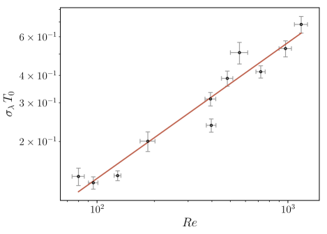
Figure 9: Data and linear fit to determine power law $\sigma_{\lambda}T_{0}\sim\text{Re}^{\gamma}$

III.4 Effect of definition of $T_{0}$ on $\alpha$

We note that previous results which have analyzed the relationship in Equation (2) have found disagreement in the value of $\alpha$ which they produce. For example, previous results using the direct method for DNS have given an $\alpha=0.53\pm 0.03$ Berera and Ho (2018), which agrees with the finding using an FTLE method as done here. However, other FTLE DNS results have found $0.64\pm 0.05$ Boffetta and Musacchio (2017). This section offers a resolution to this discrepancy in the results.

One of the main features of turbulence is that it involves many characteristic scales. Furthermore, in homogeneous and isotropic turbulence, the absence of boundary conditions sets an extra complication in determining the large scale quantities. Using different definitions of the large length and time scales can result in different analyses. The key difference between the prior works was that these used different choices for the definition of $L$ and $T_{0}$. In Berera and Ho (2018), $L$ is the integral length scale defined in section I and $T_{0}=L/U$, whereas in Boffetta and Musacchio (2017), this value was defined differently, being $T_{E0}=E/\varepsilon$ and then $L_{E}=UT_{E0}$. The forcing used in Berera and Ho (2018) was the same used in this work and the same as used in Boffetta and Musacchio (2017).

The difference between these definitions deserves some attention. The definition of the integral length scale $L$ stems from the correlation function $R_{ij}(r)=\langle u_{i}(\bm{x})u_{j}(\bm{x}+\bm{r})\rangle$ and can be associated with the size of the largest eddies. Hence, the first definition, given by the integral length scale, can be understood as the average time that it takes for a large eddy initially occupying a given region is space to move to a different region which is completely uncorrelated with the initial one. The second definition $T_{E0}$ takes the total energy $E$ and the dissipation rate $\varepsilon$, which is associated with the characteristic time in which the largest eddies transfer energy to smaller eddies in the energy cascade.

Taylor in 1935 proposed the following relation for a HIT flow in a steady state, using dimensional analysis Taylor (1935),

$$\varepsilon=C_{\varepsilon}\frac{U^{3}}{L}\quad,$$ (18)

where $C_{\varepsilon}$ is known as the dimensionless dissipation rate. Evidence has shown that this coefficient tends to a constant value $C_{\varepsilon,\infty}\approx 0.5$ for high Re Doering and Constantin (1994); Sreenivasan (1998); Gotoh et al. (2002).

At this point we should note that if we compare the definitions of $T_{0}$ and $T_{E0}$ in the large Reynolds numbers limit where $C_{\varepsilon}\approx 0.5$ and using that $E=3U^{2}/2$, these two definitions differ only by a constant factor, being $T_{E0}=3T_{0}$. In such case, there should be no discrepancy when using these different definitions to test Ruelle’s relation. Nevertheless, if we consider that the dimensionless dissipation has some Reynolds number dependence, then both definitions will have an impact in the scaling relation between $\lambda$ and Re given by Eq.(2).

We can improve the accuracy of this analysis by considering a useful expression for the dimensionless dissipation rate derived by McComb et al Mccomb et al. (2015). The following expression is derived using the von Kármán-Howarth equation and performing an asymptotic expansion in the second and third-order structure functions in powers of the inverse Reynolds number, obtaining

$$C_{\varepsilon}(Re)=C_{\varepsilon,\infty}+\frac{C}{Re}+\mathcal{O}\left(\frac{1}{Re^{2}}\right)\quad,$$ (19)

where $C$ is a constant that does not depend on Re. Also in Mccomb et al. (2015), these constants are computed using DNS. The numerical values obtained are $C_{\varepsilon,\infty}=0.486\pm 0.006$ and $C=18.9\pm 1.3$, which are in agreement with other values in literature Sreenivasan (1998). Our simulations show that the relation of $C_{\varepsilon}(\text{Re})$ as a function of Re is in strong agreement with the results of Mccomb et al. (2015).

Considering this result, we see that the relation between $T_{E0}$ and $T_{0}$ carries some extra dependence on the Reynolds number,

$$T_{E0} =\frac{E}{\varepsilon}=\frac{3L}{2C_{\varepsilon}U}=\frac{3}{2C_{\varepsilon}(Re)}T_{0}\quad.$$ (20)

The scaling relation in Equation (2) is re-tested using the definition of $T_{E0}$. We expect that when we use the definition $T_{E0}$ instead of $T_{0}$, a different exponent $\alpha_{E}$ is found instead of $\alpha$. So

$$\lambda T_{E0}=D_{E}Re^{\alpha_{E}}\quad.$$ (21)

Figure 10 shows the data for $\lambda$ as a function of Re using the definition $T_{E0}$. Using a linear fit, we obtain the values for Equation (21) of $\alpha_{E}=0.658\pm 0.006$ and $D_{E}=0.101\pm 0.001$. These results are in agreement with those found in (Boffetta and Musacchio, 2017).

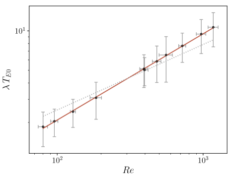
Figure 10: (Color online) $\lambda$ vs Re using the definition of $T_{E0}=E/\varepsilon$. The linear fit is indicated by a solid gray (red) line whereas Ruelle’s prediction is denoted by the dotted line.

Since the data in Figure 10 seems to be more correlated than that in Figure 7, we can take Eq.(21) as the base equation and see how it would affect Eq.(2). In this way we attempt to compare the two different definitions $T_{0}$ and $T_{E0}$. Starting from Eq.(21), the following relation is obtained

$$\lambda\overbracket{T_{0}\frac{3}{2\,C_{\varepsilon}}}^{T_{E0}} =D_{E}Re^{\alpha_{E}}\,,$$

$$\lambda T_{0} =f(Re)\equiv\frac{2D_{E}}{3}Re^{\alpha_{E}}C_{\varepsilon}(Re)\,.$$ (22)

This relation sets an extra dependence on the Reynolds number that is not present in the original Ruelle’s relation in Eq.(2). Figure 11 shows the comparison between the data obtained, Ruelle’s prediction, and the prediction given by $f($Re$)$ in Eq.(22) by using the two different definitions $T_{0}$ and $T_{E0}$. It can be seen that the slight curved deviation from the line is well predicted by $f($Re$)$.

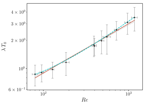
Figure 11: (Color online) Data obtained for $\lambda$ vs $T_{0}$, the straight solid gray (red) line represent the linear fit, the straight grey dotted line represents Ruelle’s prediction and the curved dashed light gray (cyan) line represents the prediction given by $f($Re$)$.

We can also predict the expected value of $\alpha$ when considering the extra Re dependence in Eq.(19) and given the measured value for $\alpha_{E}$ and see if it is consistent with the one found in the previous section. To compare both exponents, we consider equations (2) and (22). Then we take the following derivative to determine the scaling relation

$$\alpha =\frac{d\ln(\lambda T_{0})}{d\ln Re}=\alpha_{E}+Re\frac{d\ln\left(C(Re)\right)}{dRe}\quad,$$

$$\alpha =\alpha(Re)=\alpha_{E}-\frac{1}{1+\frac{C_{\varepsilon,\infty}}{C}Re}\quad.$$ (23)

As expected from Figure (11), the scaling is not a constant since it has a slight dependence on Re. To compare with the expected value of $\alpha$ previously obtained, we first evaluate $\alpha($Re$)$ using the same values of Re measured in the simulations. Then we take the average, obtaining

$$\langle\alpha\rangle_{\text{exp}}=\alpha_{E}-\left\langle\frac{1}{1+\frac{C_{\varepsilon,\infty}}{C}Re}\right\rangle\approx 0.52\quad,$$ (24)

which is within one standard deviation of the measured value of $\alpha$. This shows that both procedures are consistent. Although the data in Figure 10 is more linearly correlated. This resolves the apparent disagreement between results in Berera and Ho (2018) and Boffetta and Musacchio (2017), and is one of the main results in this paper.

We also measure the scaling relation $\sigma_{\lambda}T_{E0}\propto\text{Re}^{\gamma_{E}}$ and compare it to that found in Boffetta and Musacchio (2017). In that work, the authors claim that the uncertainty for this value is large but obtain $\gamma_{*}\sim 1.2$. In our simulations, we find a smaller value $\gamma_{E}=0.75\pm 0.05$, which is closer to the value of $0.62\pm 0.05$ for $\gamma$ found previously using the integral length scale to define $T_{0}$.

III.5 FTLE steptime dependence of $\lambda$

When the FTLE method is used, it is necessary to set certain parameters such as the magnitude of the perturbation or the steptime $\Delta t$ between successive perturbations. It is reasonable to suppose that for large values of the steptime the results are more stable since the maximal Lyapunov exponent is defined for $t\rightarrow\infty$. However, in the case of FTLEs some dependence on the initial perturbation is expected, hence, the drawback is that for finite times, i.e. $\Delta t<<2T_{E0}$, the growth might not reach stability and thus the estimate of $\lambda$ and $\sigma_{\lambda}$ might be inaccurate for reasons we give in Section IV. On the other hand, having shorter steptime would be an advantage in the sense that it allows one to obtain a larger sample of Lyapunov exponents in a significantly shorter simulation time.

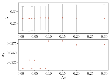
Figure 12: Dependence of $\lambda$ and $\sigma_{\lambda}$ on the steptime $\Delta t$.

Figure 12 shows the result of varying the steptime $\Delta t$ on the Lyapunov exponent and its fluctuations. The simulation has Re $=50$. As can be seen in the Figure, the values of $\lambda$ and $\sigma_{\lambda}$ are remarkably stable even for very short steptimes using the FTLE method. Indeed, at the extreme lowest value, the steptime is so short that it is only 5-10 simulation timesteps. At the other extreme, the direct method, previously described, is akin to having a very high steptime such that, within one steptime, the system becomes decorrelated. Even using the direct method, the mean values of $\lambda$ are similar to the ones found using the FTLE method.These results suggest that the steptime is of very little importance to the measured value of $\lambda$, and so it can be measured with a very low steptime which helps to reduce the computational cost. This finding can be useful in certain applications that use the Lyapunov exponent to characterize turbulent flows Nastac et al. (2017), especially if we find a way to relate the Lyapunov exponent to other quantities that characterize the flow such as Reynolds number, energy or dissipation rate. This is the main finding in this paper and together with the fast stability described in Section IV. This means that the Lyapunov exponent is a robust measure in these type of simulations.

III.6 Decaying turbulence

We analyze the chaotic behaviour in a decaying turbulent flow. The procedure consists in evolving an initial field until it enters a power law decay phase. After that, a copy of the field is created and perturbed infinitesimally. Then, we measure the evolution of the energy difference in time $E_{d}(t)$ and compare it with predictions. Using the relation in Eq.(2) for steady states, we are able to predict the evolution of $E_{d}(t)$ by adapting it to a decaying flow. For this we consider the difference field at a given simulation time $t_{i}$ as $\lvert\delta\bm{u}\left(t_{i}\right)\rvert\equiv\delta u_{i}$. For each simulation time, we assume that the difference grows exponentially. Thus we have

$$\delta u_{i+1}\approx\delta u_{i}\exp\left(\lambda_{i+1}\delta t\right)\frac{\lvert\bm{u}_{i+1}\rvert}{\lvert\bm{u_{i}}\rvert}\quad,$$ (25)

where $\delta t\equiv t_{i+1}-t_{i}$ is the timestep of the simulation. We multiply by the factor $\lvert\bm{u}_{i+1}\rvert/\lvert\bm{u_{i}}\rvert$ to account for the decay in the magnitude of $\left\lvert\bm{u}\right\rvert$, that we assume uniform. It is important to remark that this approximation also assumes that the Lyapunov exponent vary slowly in time, thus $\left(\lambda_{i+1}+\lambda_{i}\right)/2\approx\lambda_{i+1}$.

Continuing for $i+2$, we obtain

$$\delta u_{i+2}=\delta u_{i+1}\exp\left(\lambda_{i+1}\delta t+\lambda_{i+2}\delta t\right)\frac{\lvert\bm{u}_{i+2}\rvert}{\lvert\bm{u_{i}}\rvert}\quad,$$ (26)

and so, in general

$$\delta u_{f}=\delta u_{i}\exp\left(\int_{i}^{f}dt\lambda(t)\right)\frac{\lvert\bm{u}_{f}\rvert}{\lvert\bm{u_{i}}\rvert}\quad,$$ (27)

where we replace the infinite sum for the integral over time, and $\lambda(t)$ is a function of time.

We use this prediction to discriminate between the different functional dependencies of $\lambda$ given in Eqs. (2) and (21). This is a convenient comparison method because the predicted value of $\delta u_{f}$ in Eq.(27) is very sensitive to changes in $\lambda(t)$. Using these laws and the statistical properties of the unperturbed field, we can numerically perform the integral in Eq.(27) without having to measure Lyapunov exponents in the decaying regime. Thus, we predict the behaviour of $E_{d}(t)$ given its initial value $E_{d}(10)$. We use a simulation with $N=1024^{3}$ and we perturb the flow at wavenumber $k=40$.

Figure 13 shows the influence of the different functional forms of $\lambda$ using Eq.(27) to predict $E_{d}(t)$ as well as the measured value of $E_{d}(t)$ for the above mentioned simulation. As can be seen, the prediction given by (21), that uses $T_{E0}$ as the large time scale is the best fit to the measured data. This fit can be improved by using slightly higher values of $D_{E}$ and $\alpha_{E}$, which would still be within one standard deviation of the fit for the forced data. This is further evidence that the functional form of $\lambda$ predicted by Eq.(21) is the best fit to data. This has implications for the physical origin of the Eulerian chaos in turbulence, since we cannot derive Eq.(21) from the prediction $\lambda\sim 1/\tau$ consistently with the Kolmogorov theory. As such, chaos in HIT must have some different physical basis.

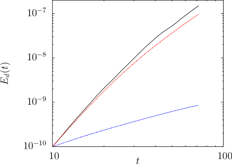
Figure 13: Different predictions of the functional form for $\lambda$. The red dotted line corresponds to the prediction in (21) the blue dotted line to the prediction in (2). The solid black line corresponds to the measured data.

IV Timescales in HIT

Quantities such as energy, Reynolds number, Lyapunov exponents and dissipation rate fluctuate around a mean value during a steady state. We look at the timescales of these time signals produced in our simulations. Especially we look at the fluctuations in the Lyapunov exponent and we compare it with those of energy and dissipation rate. One of the interesting features noted in Mohan et al. (2017) is that the fluctuations in the Lyapunov exponents are faster than those of energy or dissipation rate. This can occur due to the perturbation we introduce every steptime $\Delta t$. Here a more systematic study of this timescale is presented. We observed the autocorrelation of the signal to measure its self-decorrelation time, which we will simply call decorrelation time. Given the above findings that histograms for some magnitudes reach a stable distribution faster than for others, we may wonder what is the run time necessary to get a stable measurement of different variables depending on the timescale inherent in each time signal. In order to determine such time, it is useful to look at the decorrelation time.

Previous results show that $E_{ud}$ has a limit to its growth rate which is roughly equal to $\varepsilon$ Berera and Ho (2018). We also know that the value of $E_{ud}$ saturates at $2E$ As such, the minimum time that it takes for two fields to become completely decorrelated is $2E/\epsilon=2T_{E0}$. This result means that the timescale that is relevant for the energy and other large scale properties are dependent on $T_{E0}$.

For this purpose, we use the autocorrelation in time $\rho_{X,\Delta t}$ for some random variable $X$. The autocorrelation is related to the covariance $\rho_{X,Y}$, defined as

$$\rho_{X,Y}=\frac{E[(X-\mu_{X})(Y-\mu_{Y})]}{\sigma_{X}\sigma_{Y}}\ ,$$ (28)

where $E[...]$ is the expectation, $Y$ is some random variable, $\mu$ is the mean, and $\sigma$ the standard deviation. If we then define $Y$ as the value of $X$ after some time $\Delta t$ (in this section $\Delta t$ is not related in anyway to the steptime $\Delta t$ used in previous sections), then we can define $\rho_{X,\Delta t}$ as equivalent to $\rho_{X,Y}$ here. In this case, $X$ and $Y$ should have the same statistics, and so the equation simplifies to

$$\rho_{X,\Delta t}=\frac{E[XX_{\Delta t}]-\mu_{X}^{2}}{Var[X]}\ ,$$ (29)

where $X_{\Delta t}$ is the value of $X$ after time $\Delta t$, and $Var[...]$ is the variance.

We perform simulations of forced HIT using a value of $\nu=0.006$ on a lattice of size $128^{3}$ with $\varepsilon=0.1$. The simulations had $T_{E0}=5.43$ in simulation time units, with Re $=130$. In this instance, we run it until simulation time 1000, which is over 450 large eddy turnover times.

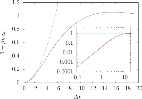
Figure 14: Solid line shows complementary autocorrelation of energy $1-\rho_{E,\Delta t}$ for Re $=130$. Dashed line shows scaling with $(\Delta t)^{2}$, dotted line shows constant 1. Inset is same as main plot but with log-log axes.

Figure 14 shows $(1-\rho_{E,\Delta t})$ for the simulation described in the previous paragraph. For small $\Delta t$ we can approximate $1-\rho_{E,\Delta t}=(\Delta t/T_{d})^{2}$, where we define $T_{d}$ as the characteristic decorrelation time. In this case, we find that $T_{d}=5.55$, which is very close to the measured value of $T_{E0}$. Similarly, we find that the point at which $\rho_{E,\Delta t}=0$ is at $\Delta t=11.48$, which agrees with our prediction that the time for two fields to become completely decorrelated is roughly $2T_{E0}$. We expect that the important timescale for measurement may depend on the length scale which is most important for those statistics. For instance, whilst total energy will be dominated by large scale structures, the dissipation should be dominated by the smallest lengthscales. Figure 15 shows $1-\rho_{\varepsilon,\Delta t}$ for the same simulation. Approximating $1-\rho_{\varepsilon,\Delta t}=(\Delta t/T_{d})^{2}$ gives $T_{d}=2.58$, which is approximately half the value of $T_{E0}$. Similarly, the time at which $\rho_{\varepsilon,\Delta t}<0$ is actually less than $T_{E0}$.

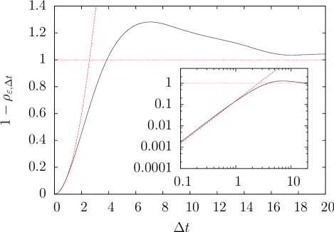
Figure 15: Solid line shows complementary autocorrelation of dissipation $1-\rho_{\varepsilon,\Delta t}$ for Re $=130$. Dashed line shows scaling with $(\Delta t)^{2}$, dotted line shows constant 1. Inset is same as main plot but with log-log axes.

We calculate the autocorrelation for $E(k)$ in order to look at the dependence on the length scale explicitly. The plot for $\rho_{E(1),\Delta t}$ looks very similar to those for $\rho_{E,\Delta t}$. However, the plots for $k>1$, even as low as $k=2$, look more like the plots for $\rho_{\varepsilon,\Delta t}$, despite the fact that $k=2$ is within the forcing range. All of these plots reach $\rho_{E(k),\Delta t}\leq 0$ quicker than $T_{E0}$ when $k>1$. For moderately high $k$, there is a $(\Delta t/T_{d})^{2}$ dependence at low $\Delta t$. But, when we look at the autocorrelation for very high wave number, something unexpected happens, which is that a new scaling appears.

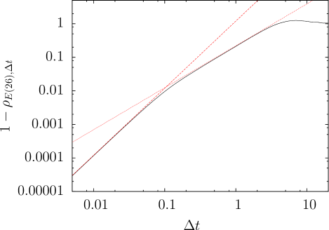
Figure 16: Solid line shows complementary autocorrelation of $E(26)$, $1-\rho_{E(26),\Delta t}$ for Re $=130$. Dashed line shows scaling with $(\Delta t)^{2}$, dotted line shows scaling with $(\Delta t)^{5/4}$.

Figure 16 shows $1-\rho_{E(26),\Delta t}$. The value $k=26$ is chosen because it is roughly the inverse of the Kolmogorov microscale for this simulation. The new scaling is approximately $(\Delta t)^{5/4}$. Even with this new scaling, the autocorrelation still becomes decorrelated before $T_{E0}$.

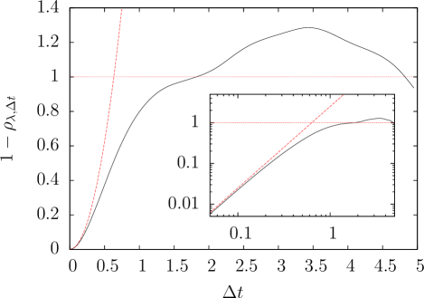
Figure 17: Solid line shows complementary autocorrelation of $\lambda$, $1-\rho_{\lambda,\Delta t}$ for Re $=130$. Dashed line shows scaling with $(\Delta t)^{2}$, dotted line shows constant 1. Inset is same as main plot but with log-log axes.

We now look at the autocorrelation for $\lambda$ itself. Figure 17 shows $1-\rho_{\lambda,\Delta t}$. These statistics are measured on a simulation with a much shorter run time and with FTLE steptime $\Delta t=0.05$. We find that $T_{d}\approx 0.5$ and the time until decorrelation is roughly $T_{0}/4$. This is further evidence that the FTLE should reach stable statistics faster than for instance, the Reynolds number or total energy. This is one of the main results in this paper. We may expect this longer correlation time for the statistics like total energy, Re, and dissipation compared to the Lyapunov exponent just from looking at their evolution in time. The graphs for Lyapunov exponent fluctuate more wildly. The correlation between Lyapunov exponents has a much shorter timescale which is why the statistics of the Lyapunov exponent are more quickly approximated by a Gaussian. However, the Lyapunov exponent becomes decorrelated even faster than the energy at the Kolmogorov microscale, even though we would expect those scales to be evolving the fastest in the whole system. This might indicate that the perturbations introduced in the FTLE method have a relevant effect on the Lyapunov exponent self-correlation time. However we cannot consider successive values of $\lambda$ to be uncorrelated since the decorrelation timescale $T_{d}$ is much larger than the steptime.

Given the decorrelation time $T_{d}$, we need to determine the run time $T_{r}$ necessary to obtain proper statistics for each quantity. It is important to mention that $T_{r}$ is not the actual run time of the simulation but the time in which the simulation is in the steady state, so initial transients are not considered.

For this purpose, a useful quantity to look at is the standard error of the mean $\sigma_{\overline{X}}$. We may consider a set of measurements of a quantity $X$, with its own mean $\overline{X}$ and standard deviation $\sigma$. If instead, we consider a subset of $n$ measurements, we can measure a mean value of $X$ ($\overline{X}_{\text{sub}}$) that will usually differ from the real mean value $\overline{X}$. Repeating this procedure many times for different subsets, we can get a distribution of $\overline{X}_{\text{sub}}$. The standard deviation of such a distribution is defined as the standard error of the mean $\sigma_{\overline{X}}$. It is known that for Gaussian distributions, the relation $\sigma_{\overline{X}}/\sigma=1/\sqrt{n}$ holds, where $\sigma$ is the standard deviation of the entire set, so as $n$ grows, the estimate of the mean improves.

To associate the value of $n$ to the time signals obtained in our simulations, we divided the entire run time in $n$ segments of length given by the decorrelation time $T_{d}$, so $n=T_{r}/T_{d}$, then, the relation between the standard error of the mean and the standard deviation is now

$$\frac{\sigma_{\overline{X}}}{\sigma}=\sqrt{\frac{T_{d}}{T_{r}}}\quad,$$ (30)

where $\sigma$ is now the standard deviation of the signal in a simulation with $T_{r}\rightarrow\infty$. As a rule of thumb, the standard error of the mean should be no greater than $10\%$ of the standard deviation, so a value of $T_{r}\approx 100T_{d}$ will ensure this condition. That is the reason why in the case of measuring Lyapunov exponents, for which $T_{d}\approx 0.5\approx T_{E0}/10$, a run time of $T_{r}=50\approx 10T_{E0}$ is enough to obtain proper statistics, whereas for the energy, that same run time is not enough. Note that the above criteria to determine the run time is uniquely dependent on the decorrelation time, since it is not necessary to measure $\sigma$ and $\sigma_{\overline{X}}$ once we observe that the distribution is approximately Gaussian.

On the other hand, the proper run time needed to obtain proper statistics for the energy is approximately $100\,T_{E0}$, which is ten times greater than that needed in the case of Lyapunov exponents. The measurement of Lyapunov exponents are the most robust in these simulations. This suggests that the Lyapunov exponents are not only stable to variations in the steptime and lattice size, but also the run time needed to compute them is much faster than for other flow quantities. Thus, using relations such as Ruelle’s, that connect the Lyapunov exponent to Reynolds number, is useful to attempt to characterize the flow in a quick and robust way.

V MHD

$N^{3}$	$\nu$	$\varepsilon$	Re	$\lambda$	$\sigma_{\lambda}$	$T_{0}$	$\tau$	$k_{\text{max}}\eta$
643	0.0200	0.084	44.0	0.284	0.031	3.041461	0.488	1.98
1283	0.0100	0.062	84.0	0.282	0.051	2.891003	0.402	2.60
1283	0.0080	0.055	109.0	0.275	0.046	2.875559	0.380	2.26
1283	0.0060	0.048	139.0	0.312	0.048	2.912633	0.353	1.89
1283	0.0040	0.039	201.0	0.302	0.059	2.940972	0.320	1.47
2563	0.0020	0.032	397.0	0.336	0.068	3.022230	0.251	1.88
2563	0.0018	0.031	462.0	0.351	0.055	3.008904	0.241	1.75
2563	0.0016	0.031	500.0	0.363	0.073	2.989567	0.227	1.60
2563	0.0014	0.031	545.0	0.382	0.114	2.938673	0.214	1.45
5123	0.0010	0.029	786.0	0.365	0.070	3.158999	0.187	2.31
5123	0.0008	0.028	1089.0	0.414	0.049	3.205189	0.170	1.97
5123	0.0006	0.029	1342.0	0.461	0.055	2.940171	0.145	1.58

Table 2: Simulation parameters for 12 MHD simulations. N is the lattice size, $\nu$ is the kinematic viscosity, $\epsilon$ is the kinematic dissipation rate, Re is the Reynolds number, $\lambda$ is the maximal Lyapunov exponent and $\sigma_{\lambda}$ its standard deviation, $T_{0}$ is the large eddy turnover time, $\tau$ is the Kolmogorov microscale time, $k_{\text{max}}\approx N/3-1$ is the maximum resolved wavenumber, $\eta=(\nu^{3}/\varepsilon)^{1/4}$ is the Kolmogorov microscale length and $k_{\text{max}}\eta$ is the resolution.

Twelve simulations were run using the incompressible MHD equations described in Equations (6 - 7). These simulations keep magnetic Prandtl number, Pm $=\nu/\eta$, set to 1 for all simulations. The forcing is set so that the sum of magnetic and kinetic dissipation is approximately 0.1 and magnetic helicity is kept low. The FTLE method was used to obtain the Lyapunov exponents. The values of Re ranged between 40 and 1300. Figure 18 shows histograms for the distribution of $\lambda$ and Re obtained from one of the simulations. Table 2 shows parameter values for all simulations. Similar to the hydrodynamic case, whilst the $\lambda$ are well approximated by a Gaussian distribution, the value for Re is not. As is known, analysis of the chaotic properties of MHD simulations presents noisier results than the NSE case Ho et al. (2019). As well, we find that characteristic quantities and their fluctuations are less correlated. MHD involves more time and length scales than magnetically neutral flows, given that for each velocity field length and time scale, there is a corresponding time or length scale for the magnetic field. As well, there are new relations between these scales that are possible given the presence of magnetic diffusion. Hence, it is to be expected that some dependencies that are obtained from dimensional considerations in hydrodynamics are lost in MHD.

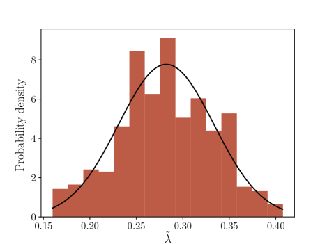
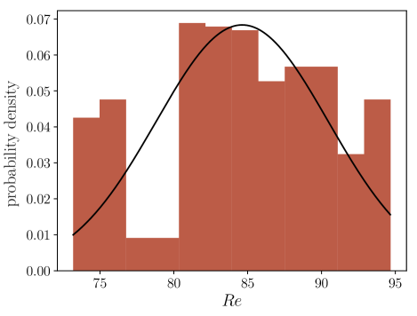
Figure 18: Distributions of $\lambda$ and Re for the MHD case for one simulation.

The first relationship to test for MHD simulations is the Ruelle relation $\lambda\propto 1/\tau$. Here, $\tau=(\nu/\epsilon)^{1/2}$ is the Kolmogorov time, and the dissipation is the kinetic dissipation. Figure 19 shows $\lambda$ against $1/\tau$. A linear fit $\lambda=A+B\tau^{-1}$ is done. The measured values are $A=0.19\pm 0.02$ and $B=0.037\pm 0.004$. Nevertheless, in Ho et al. (2019) the same plot is presented for a wider range of values of $\tau^{-1}$, showing that for the values of $\tau^{-1}$ we explore, the linear approximation is not accurate whereas for those values that are not explored here the linear approximation becomes reasonable. Exploring a wider range of values to evaluate this relation is not the main goal of this project and that would require computational cost which is not pursued for this work.

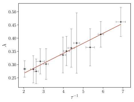
Figure 19: $\lambda$ vs $\tau^{-1}$ (the inverse of Kolmogorov time $\tau=(\nu/\epsilon)^{1/2}$) and linear fit represented by the solid red line.

Figure 20 shows the relationship between $\lambda$ and Re. This plot allows us to test the scaling relation in Equation (2). From the Figure, we measure a value of $\alpha=0.14\pm 0.02$, which is quite far from the value of $\alpha\approx 0.5$ found previously for hydrodynamic simulations. The derivation of Eq.(2) relies strongly on the fact that the characteristic quantities of the flow at different scales are less ambiguous in hydrodynamics, whilst for MHD, many other quantities such as magnetic diffusion or magnetic field length and time scales bring more ambiguity in the dimensional analysis. The correlation observed between $\sigma_{\lambda}$ and Re is very weak, contrary to the hydrodynamic case, where there was a strong correlation as is shown in Figure 9.

Figure 20: $\lambda T_{0}$ vs. Re using the FTLE method in a MHD fluid

We now compare the dependence of $\sigma_{\lambda}$ on $\lambda$ and $\sigma_{\text{Re}}$ on Re, as was done for hydrodynamics previously. Figure 21 shows these relations for our MHD simulations. There are similarities and differences with the hydrodynamic results. Unlike for NSE, in MHD the fluctuations in the Lyapunov exponents are not strongly related to $\lambda$. However, similar to the NSE case, in MHD the fluctuations of Re are strongly related to Re itself. From the Figure, a linear fit for the MHD simulations of $\sigma_{\text{Re}}=c_{3}\text{Re}$ results in a measured value for the slope of $c_{3}=0.052\pm 0.006$. This value is of the same order of the analogous slope for hydrodynamics $c_{1}=0.08\pm 0.01$.

The fact that the relation between Re and its fluctuations are similar for both NSE and MHD runs shows that this relation is probably a characteristic of the forced equations. Although in both MHD and hydrodynamics, the relationship between $\lambda$ and $1/\tau$ is strong, the strong relationship between $\tau$ and Re only holds in hydrodynamics. Since these relations are not uniquely determined in MHD, the behavior of $\lambda$ is not as strongly related to Re. The lack of a uniquely determined relation may be the reason why the linear relation between $\sigma_{\lambda}$ and $\lambda$ is not present in MHD.

Figure 21: Distributions of $\lambda$ and Re for the MHD case. No correlation was shown between $\lambda$ and $\sigma_{\lambda}$. The relation between Re and its fluctuations presented a linear relation with a fit given by the solid line.

Similar to hydrodynamics, we test the sensitivity of the MHD FTLE results to changes in steptime. Figure 22 shows the dependence of $\lambda$ and $\sigma_{\lambda}$ on the steptime $\Delta t$ of the FTLE method for one MHD simulation. As in the hydrodynamic case, both $\lambda$ and $\sigma_{\lambda}$ seem to be stable even though a very wide range of $\Delta t$ is explored.

Figure 22: Dependence of $\lambda$ and $\sigma_{\lambda}$ on the steptime $\Delta t$ of the FTLE method for MHD flows.

VI Discussion and conclusions

We studied Eulerian chaos in homogeneous and isotropic flows evolved using the incompressible Navier-Stokes equations. We observed the finite time Lyapunov exponents and the dependence of fluctuations on other parameters such as Reynolds number, lattice size and steptime in the FTLE procedure. There are four main results which we may take from the analysis done in this paper.

The first is that the FTLEs are approximately Gaussian distributed. We do not expect that they are fully Gaussian however, because the statistics on which it depends, and turbulent statistics in general, are known to be non-Gaussian.

We may try to find out the true distribution of the FTLEs by relating it to previous results found by analysing HIT with dynamical systems theory. Previously, it has been found that when the NSE are modelled with a negative damping force, at low Re a relaminarization process occurs akin to that found in parallel wall-bounded shear flows Linkmann and Morozov (2015). The lifetime of this process was found to depend super-exponentially on the Reynolds number. We can associate the parts of the distribution of the FTLE where $\lambda<0$ with laminar regions of the state space. The proportion of the total state space which is laminar can be calculated using the cumulative distribution function (CDF) and substitute the dependence on Re of the distribution into this CDF. If we approximate the FTLE as being totally decorrelated, we can associate the relaminarization rate with the rate at which the FTLE becomes negative. The CDF of a Gaussian distribution follows a complementary error function. Substituting the values in this paper to generate a Re dependence for the relaminarization rate does not generate the super exponential rates found previously in turbulence Linkmann and Morozov (2015). Motivated by this finding, we could modify the probability distribution of the FTLEs and perhaps use some form of generalized extreme value distribution, which have CDFs which are super exponential in form. However, the situation may be much more subtle and require further analysis than the one outlined briefly here.

The second finding relates to the most important time scale for chaos in HIT. We may begin to question whether the relationship derived by Ruelle is the fundamental one or whether it is actually a consequence of the relationship in Eq.(21) being the fundamental one. If Eq.(21) were the fundamental relationship, it would support the idea that the true timescale for the chaotic properties is $E/\varepsilon$ rather than $L/U$. The study of the chaotic behaviour in decaying turbulence shows that the evolution of the divergence is quite sensitive to the different functional forms proposed. Numerical data supports the idea that $E/\varepsilon$ is the one that best fit the data. We also see that the lattice size is not really a factor, and under-resolved simulations also capture the chaotic behaviour. As such, the smallest length scales may not be as relevant to the chaos and as shown in previous works Berera and Ho (2018); Boffetta and Musacchio (2017); Mukherjee et al. (2016), these are the scales in which the two field initially close become decorrelated first. Conversely, large scale properties take a longer time to decorrelate and thus are more predictable.

Third, from the analysis of Figure 12, we see that both the Lyapunov exponent and its fluctuations are very weakly dependent on the steptime used in the FTLE method. Practically, this result means that the time needed to get a measure of this chaotic property can be achieved at low computational cost.

Fourth, motivated by understanding the chaotic properties of the system, we analyzed the timescale of the signals of the energy, dissipation rate and Lyapunov exponent in the steady state. We look at the time autocorrelation and we see that the energy only becomes decorrelated after $2T_{E0}$. However, the small scale properties become decorrelated faster than $T_{E0}$ and the Eulerian maximal Lyapunov exponent becomes decorrelated faster than any of these other statistics, suggesting that it is the most robust to measurement in simulations, reaching a faster stability. From this analysis we obtain a useful rule that determines the run time $T_{r}$ needed to obtain proper statistics of a quantity by considering the decorrelation time in its signal $T_{d}$, being $T_{r}\approx 100\,T_{d}$. For instance, we see that for the total energy, averages need to be taken for run times $T_{r}\approx 100T_{E0}$, whereas for other properties such as Lyapunov exponents or dissipation rate, shorter run times can be used. This run time rule we give in relation to the self correlation time is useful not only when looking at chaotic properties of the flow but also for any other study that needs to measure quantities in the steady state.

The robustness of the results when measuring the maximal Lyapunov exponent suggest that it is a stable statistical property of the system. We also see that it reaches stability faster than other statistical properties of the system and our analysis cements it as an extra parameter of HIT which is important in understanding the interesting inter-scale dynamics inherent in turbulent flows. This could have further applications in studies that use the Lyapunov exponent to characterize the turbulent flow as in Nastac et al. (2017). Furthermore, if we learn the relation between the Lyapunov exponent and other flow quantities, we could use such an exponent to determine these other quantities in a faster and more stable way. For instance, Ruelle’s relation relates $\lambda$ and Re and this can be used to estimate Re in a shorter run time.

Finally, in this paper some of the FTLEs’ properties measured for hydrodynamic flows were measured for the case of isotropic and incompressible MHD flows. The distribution of FTLEs is approximately Gaussian as in the case of NSE. The remarkable stability of FTLEs against variations in the steptime is also present in MHD flows. Nevertheless, the dependence on Reynolds number is not the same as in the case of NSE. Ruelle’s relation is derived from assuming that the Kolmogorov time is the smallest timescale in the system. Whereas this is true for incompressible NSE, other characteristic timescales are present in the smallest scales in MHD that may break this relation.

References

- Ruelle and Takens (1971) D. Ruelle and F. Takens, Comm. Math. Phys. 20, 167 (1971).
- Deissler (1986) R. Deissler, Phys. Fluids 29, 1453 (1986).
- Lorenz (1963) E. N. Lorenz, J. Atmospheric Sci. 20, 130 (1963).
- Yoden and Nomura (1993) S. Yoden and M. Nomura, J. Atmospheric Sci. 50, 1531 (1993).
- Masuoka et al. (2003) T. Masuoka, Y. Takatsu, and T. Inoue, Microscale Thermophys. Eng. 6, 347 (2003).
- Musker (1979) A. Musker, AIAA J. 17, 655 (1979).
- Poirel and Price (2001) D. C. Poirel and S. J. Price, AIAA J. 39, 1960 (2001).
- Leith (1971) C. Leith, J. Atmospheric Sci. 28, 145 (1971).
- Leith and Kraichnan (1972) C. Leith and R. Kraichnan, J. Atmospheric Sci. 29, 1041 (1972).
- Aurell et al. (1997) E. Aurell, G. Boffetta, A. Crisanti, G. Paladin, and A. Vulpiani, J. Phys. A: Math. Gen. 30, 1 (1997).
- Kurths and Herzel (1986) J. Kurths and H. Herzel, Sol. Phys. 107, 39 (1986).
- Grappin et al. (1986) R. Grappin, J. Leorat, and A. Pouquet, J. de Physique 47, 1127 (1986).
- Huang et al. (1994) W. Huang, W. Ding, D. Feng, and C. Yu, Phys. Rev. E 50, 1062 (1994).
- Berera and Ho (2018) A. Berera and R. D. J. G. Ho, Phys. Rev. Lett. 120, 024101 (2018).
- Boffetta and Musacchio (2017) G. Boffetta and S. Musacchio, Phys. Rev. Lett. 119, 054102 (2017).
- Mohan et al. (2017) P. Mohan, N. Fitzsimmons, and R. D. Moser, Phys. Rev. Fluids 2, 114606 (2017).
- Ho et al. (2019) R. D. Ho, A. Berera, and D. Clark, Phys. Plasmas 26, 042303 (2019).
- Nastac et al. (2017) G. Nastac, J. W. Labahn, L. Magri, and M. Ihme, Phys. Rev. Fluids 2, 094606 (2017).
- Mukherjee et al. (2016) S. Mukherjee, J. Schalkwijk, and H. J. Jonker, J. Atmospheric Sci. 73, 2715 (2016).
- Li et al. (2019) Y. C. Li, R. D. Ho, A. Berera, and Z. Feng, arXiv preprint arXiv:1908.04838 (2019).
- Boffetta et al. (1997) G. Boffetta, A. Celani, A. Crisanti, and A. Vulpiani, Phys. Fluids 9, 724 (1997).
- Boffetta and Musacchio (2001) G. Boffetta and S. Musacchio, Phys. Fluids 13, 1060 (2001).
- Métais and Lesieur (1986) O. Métais and M. Lesieur, J. Atmospheric Sci. 43, 857 (1986).
- Crisanti et al. (1993) A. Crisanti, M. Jensen, A. Vulpiani, and G. Paladin, Phys. Rev. Lett. 70, 166 (1993).
- Yamada and Saiki (2007) M. Yamada and Y. Saiki, Nonlinear Process. Geophys. 14, 631 (2007).
- de Divitiis (2018) N. de Divitiis, Adv.Math. Phys. 2018 (2018).
- Lapeyre (2002) G. Lapeyre, Chaos: An Interdiscip. J. NonlinearSci. 12, 688 (2002).
- Biferale et al. (2005a) L. Biferale, G. Boffetta, A. Celani, B. Devenish, A. Lanotte, and F. Toschi, Phys. Fluids 17, 115101 (2005a).
- Biferale et al. (2005b) L. Biferale, G. Boffetta, A. Celani, B. Devenish, A. Lanotte, and F. Toschi, Phys. Fluids 17, 111701 (2005b).
- Vannitsem (2017) S. Vannitsem, Chaos: An Interdiscip. J. NonlinearSci. 27, 032101 (2017).
- Guo et al. (2016) H. Guo, W. He, T. Peterka, H.-W. Shen, S. M. Collis, and J. J. Helmus, IEEE Trans. Vis. Comput. Graph. 22, 1672 (2016).
- Garaboa-Paz et al. (2017) D. Garaboa-Paz, J. Eiras-Barca, and V. Pérez-Muñuzuri, Earth Syst. Dyn. 8, 865 (2017).
- d’Ovidio et al. (2004) F. d’Ovidio, V. Fernández, E. Hernández-García, and C. López, Geophys. Res. Lett. 31 (2004).
- Haller and Sapsis (2011) G. Haller and T. Sapsis, Chaos: An Interdiscip. J. NonlinearSci. 21, 023115 (2011).
- Haller (2015) G. Haller, Annu. Rev. Fluid Mech. 47, 137 (2015).
- Abraham and Bowen (2002) E. R. Abraham and M. M. Bowen, Chaos: An Interdiscip. J. NonlinearSci. 12, 373 (2002).
- Chian et al. (2019) A. C.-L. Chian, S. S. Silva, E. L. Rempel, M. Gošić, L. R. B. Rubio, R. A. Miranda, and I. S. Requerey, arXiv:1904.08472 (2019).
- Rempel et al. (2016) E. Rempel, A.-L. Chian, F. J. Beron-Vera, S. Szanyi, and G. Haller, Mon. Notices Royal Astron. Soc. 466, L108 (2016).
- Chian et al. (2014) A. C.-L. Chian, E. L. Rempel, G. Aulanier, B. Schmieder, S. C. Shadden, B. T. Welsch, and A. R. Yeates, The Astrophys. J 786, 51 (2014).
- Tang et al. (2012) J.-N. Tang, C.-C. Tseng, and N.-F. Wang, Acta Mech. Sin. 28, 612 (2012).
- Pedersen et al. (1996) T. S. Pedersen, P. K. Michelsen, and J. J. Rasmussen, Phys. Plasmas 3, 2939 (1996).
- Padberg et al. (2007) K. Padberg, T. Hauff, F. Jenko, and O. Junge, New J. Phys. 9, 400 (2007).
- Falessi et al. (2015) M. Falessi, F. Pegoraro, and T. Schep, J. Plasma Phys. 81 (2015).
- Misguich et al. (1987) J. Misguich, R. Balescu, H. Pecsell, T. Mikkelsen, S. Larsen, and Q. Xiaoming, Plasma Phys. Control. Fusion 29, 825 (1987).
- Shadden et al. (2005) S. C. Shadden, F. Lekien, and J. E. Marsden, Phys. D: Nonlinear Phenom. 212, 271 (2005).
- Johnson and Meneveau (2015) P. L. Johnson and C. Meneveau, Phys. Fluids 27, 085110 (2015).
- Shimada and Nagashima (1979) I. Shimada and T. Nagashima, Prog. Theor. Exp. Phys. 61, 1605 (1979).
- Ruelle (1979) D. Ruelle, Phys. Lett. A 72, 81 (1979).
- Kolmogorov (1991) A. N. Kolmogorov, Proc. Royal Soc. Lond. A 434, 15 (1991).
- Mccomb et al. (2015) W. D. Mccomb, A. Berera, S. R. Yoffe, and M. F. Linkmann, Phys. Rev. E 91 (2015).
- Machiels (1997) L. Machiels, Phys. Rev. Lett. 79, 3411 (1997).
- Ishihara and Kaneda (2003) T. Ishihara and Y. Kaneda, in Statistical Theories and Computational Approaches to Turbulence (Springer, 2003) pp. 177–188.
- Yoffe (2013) S. R. Yoffe, arXiv:1306.3408 (2013).
- Brunton and Rowley (2010) S. L. Brunton and C. W. Rowley, Chaos: An Interdiscip. J. NonlinearSci. 20, 017503 (2010).
- Oseledets (1968) V. I. Oseledets, Trans. Moscow Mater. Soc. 19, 179 (1968).
- Goldhirsch et al. (1987) I. Goldhirsch, P.-L. Sulem, and S. A. Orszag, Phys. D: Nonlinear Phenom. 27, 311 (1987).
- Taylor (1935) G. I. Taylor, Proc. Royal Soc. Lond. A 151, 421 (1935).
- Doering and Constantin (1994) C. R. Doering and P. Constantin, Phys. Rev. E 49, 4087 (1994).
- Sreenivasan (1998) K. R. Sreenivasan, Phys. Fluids 10, 528 (1998).
- Gotoh et al. (2002) T. Gotoh, D. Fukayama, and T. Nakano, Phys. Fluids 14, 1065 (2002).
- Linkmann and Morozov (2015) M. F. Linkmann and A. Morozov, Phys. Rev. Lett. 115, 134502 (2015).