Time-dependent AMS-02 electron-positron fluxes in an extended force-field model

Abstract

The magnetised solar wind modulates the Galactic cosmic ray flux in the heliosphere up to rigidities as high as 40 GeV. In this work, we present a new and straightforward extension of the popular, but limited force-field model, thus providing a fast and robust method for phenomenological studies of Galactic cosmic rays. Our semi-analytical approach takes into account charge-sign dependent modulation due to drifts in the heliospheric magnetic field and has been validated via comparison to a fully numerical code. Our model nicely reproduces the time-dependent AMS-02 measurements and we find the strength of diffusion and drifts to be strongly correlated with the heliospheric tilt angle and magnitude of the magnetic field. We are able to predict the electron and positron fluxes beyond the range for which measurements by AMS-02 have been presented. We have made an example script for the semi-analytical model publicly available and we urge the community to adopt this approach for phenomenological studies.

Introduction.—Upon entering the heliosphere, Galactic cosmic rays encounter the magnetised solar wind and are thus subject to a number of transport processes: advection with the wind, diffusion in the small-scale turbulent magnetic field, drifts due to variations of the large-scale field and adiabatic energy losses in the expanding flow. Together, these effects suppress the fluxes of cosmic rays at Earth compared to the interstellar fluxes. Collectively this is referred to as solar modulation. (See Ref. Potgieter (2013) for a review.)

For the modelling of solar modulation, two approaches have been adopted in the literature: Numerical codes solve the transport equation for models of the heliosphere of varying sophistication Kappl (2016); Vittino et al. (2018); Boschini et al. (2018); Aslam et al. (2019) and have been successfully applied to time-dependent data, too (e.g. Potgieter et al. (2015); Jerome Boschini et al. (2019); Corti et al. (2019)). While such approaches have the potential to reproduce observations elsewhere in the heliosphere and thus provide a more global picture, the complexity comes at the price of a large number of unknown parameters. These parameters need to be determined by fitting the models to various observables. However, as the input interstellar fluxes depend also on unknown parameters, running such global fits is prohibitively expensive.

Phenomenological studies of Galactic cosmic ray transport on the other hand oftentimes employ the classic force-field model of Gleeson and Axford Gleeson and Axford (1968a). This model is conceptually simple and all the complexity of the heliosphere is condensed into only one parameter, the Fisk potential, which can be easily determined by fitting to data. In addition, allowing for this electro-static potential to be time-dependent, some degree of correlation with solar activity can be found. On the downside, the force-field model assumes a higher degree of symmetry and ignores transport processes that must be important, in particular drifts. Most importantly, the force-field model has trouble reproducing the measured fluxes. One example is crossing of fluxes, e.g. the proton fluxes measured by AMS-02 during Bartels rotations  2460 and 2476 cross at $4\,\text{GeV}$ Cuoco et al. (2019). In the force-field model, fluxes modulated with different potentials differ at all energies and never cross.

A number of authors have tried to allow for more freedom while maintaining the simplicity of the force-field model, for instance by making the force-field potential rigidity-dependent Cholis et al. (2016); Gieseler et al. (2017). While interesting, these approaches are phenomenological fixes and have not been shown to derive from more fundamental principles, for instance from a transport equation. Here, we follow a different approach and present a systematic extension of the conventional force-field model. We start from the general transport equation in 2D that includes drifts and then reduce it–under a limited number of assumptions–to a force-field like structure. Our semi-analytical model allows calculating the modulated fluxes of any cosmic ray species at a very moderate computational cost. Our model contains two free parameters per time interval which we determine by fitting to the AMS-02 data. We further investigate temporal correlations with solar wind parameters and replace the free parameters by a linear model of tilt angle and magnetic field strength. Combining the semi-analytical model with the solar wind correlations allows reproducing the AMS-02 data and predicting electron and positron fluxes beyond the range of measurements by AMS-02.

Given its simplicity and speed, our semi-analytical model is bridging the gap between the oversimplified classical force-field model and the computationally expensive and unwieldy numerical codes. Therefore, it is ideally suited for fast likelihood evaluations and we urge the community to adopt it for phenomenological studies. We have made an example script for the semi-analytical model available in both Python and C++ at https://git.rwth-aachen.de/kuhlenmarco/effmod-code.

Semi-analytical model—The propagation of cosmic rays in the heliosphere is generally described in terms of a transport equation,

$$\frac{\partial f}{\partial t}+\nabla\cdot\left(C{\mathbf{V}}f-K\cdot\nabla f\right)+\frac{1}{3p^{2}}\frac{\partial}{\partial p}\left(p^{3}{\mathbf{V}}\cdot\nabla f\right)=q\,,$$ (1)

where $f$ is the cosmic ray phase space density with momenta $p$ measured in the observer frame, $C=-(\partial f/\partial p)/3$ is the Compton-Getting factor Compton and Getting (1935), ${\mathbf{V}}$ denotes the solar wind velocity, $K$ is the diffusion tensor, the third term on the left hand side describes the adiabatic losses in the expanding solar wind and $q$ is a source term.

We assume a steady state and follow the conventional force-field approach insofar as we ignore the adiabatic energy losses in the fixed frame Caballero-Lopez and Moraal (2004). Note that although we will be illustrating our method on electron and positron fluxes, all of the assumptions made are applicable for arbitrary charges and masses, that is including both non-relativistic and relativistic cosmic rays. In the absence of sources the streaming $(C{\mathbf{V}}f-K\cdot\nabla f)$ is thus divergence-free and its integral over an arbitrary surface must vanish. After some manipulations  this leads to a partial differential equation for $\tilde{f}=\tilde{f}(r,p)$

$$\frac{\partial\tilde{f}}{\partial r}+\frac{p\tilde{V}}{3\tilde{K}_{rr}}\frac{\partial\tilde{f}}{\partial p}=\frac{\tilde{v}_{gc,r}}{\tilde{K}_{rr}}\tilde{f}\,,$$ (2)

where tildes denote (weighted) polar angle averages and $\tilde{v}_{gc,r}$ is the average of the gradient curvature drift. The boundary condition is $\tilde{f}(r_{\text{max}},p)=f_{\mathrm{LIS}}(p)$, $r_{\text{max}}$ being the radius of the heliosphere. Note that absorbing the non-trivial polar angle dependencies into the averaged quantities has significantly reduced the complexity. For the same reason current sheet drifts that have the same rigidity dependence as the gradient and curvature drifts can be absorbed into the drift term. In the following, we will therefore drop the subscript ’gc’ and have $\tilde{v}_{r}$ denote a general drift term.

We can solve eq. (2) using the method of characteristics,

$$\tilde{f}(r,p)\!=\!f_{\mathrm{LIS}}(p_{\mathrm{LIS}}(r,p))\exp\left[-\int_{0}^{r}\mathrm{d}r^{\prime}\frac{\tilde{v}_{r}(r^{\prime},p_{\mathrm{LIS}}(r^{\prime},p))}{\tilde{K}_{rr}(r^{\prime},p_{\mathrm{LIS}}(r^{\prime},p)}\right]\,,$$ (3)

where we have defined $p_{\text{LIS}}(r^{\prime},p^{\prime})=p_{r^{\prime}\!,p^{\prime}}(r_{\text{max}})$ with $p_{r^{\prime}\!,p^{\prime}}(r)$ a solution of the initial value problem

$$\frac{\mathrm{d}p}{\mathrm{d}r}=\frac{p\tilde{V}}{3\tilde{K}_{rr}}\,,$$ (4)

with $p(r^{\prime})=p^{\prime}$. We stress that the functional dependence of eqs. (3) and (4) is novel and differs from the approaches of Ref. Cholis et al. (2016); Gieseler et al. (2017).

We will model only the momentum dependence of $\tilde{K}_{rr}$, $\tilde{v}_{r}$ and $\tilde{V}$ and absorb their normalisation as well as the effect of possible spatial dependencies into scaling factors by making the following replacements in eqs. (3) and (4):

$$\frac{\tilde{v}_{r}}{\tilde{K}_{rr}}\to g_{2}\frac{\tilde{v}_{r}}{\tilde{K}_{rr}}\quad\text{and}\quad\frac{p\tilde{V}}{3\tilde{K}_{rr}}\to g_{1}\frac{p\tilde{V}}{3\tilde{K}_{rr}}\,.$$ (5)

The scaling factors $g_{1}$ and $g_{2}$ will be determined by fitting to data.

Validation—In order to verify the validity of the approximations made in deriving eqs. (3) and (4), we have solved the transport eq. (1) directly using our own finite-difference code. For the numerical solution, we need to specify a particular heliospheric transport model. The model adopted is closely emulating one that has been successfully applied to data from the PAMELA experiment Potgieter et al. (2015) with some simplifications . Using the numerical code, we have confirmed that the adiabatic term, i.e. the last term on the left-hand-side of eq. (1), always contributes less than $10\,\%$ to the transport equation .

For the semi-analytical model, we adopt fiducial parametrisations for the rigidity-dependencies of $\tilde{K}_{rr}$, $\tilde{v}_{r}$ and $\tilde{V}$ that follow the rigidity-dependencies used in the numerical code. The diffusion coefficient is modelled as a softly broken power law in rigidity $R$ (understood to be measured in GV),

$$\tilde{K}_{rr}=K_{0}R^{a}\left(\frac{R^{c}+R_{k}^{c}}{1+R_{k}^{c}}\right)^{(b-a)/c}\,,$$ (6)

with a normalization $K_{0}=30\,\text{AU}^{2}/\text{d}$ , power law indices $a=0$ and $b=1.55$, $c=3.5$ and a break rigidity $R_{k}=0.28$ fixed to values obtained for electrons and positrons in previous studies Potgieter et al. (2015). The radial drift velocity can be parametrised as

$$\tilde{v}_{r}=\kappa_{\text{0}}\frac{R}{3B_{0}}\frac{10\,R^{2}}{1+10\,R^{2}}\,,$$ (7)

where we set $\kappa_{\text{0}}=1\,\text{AU}/\text{d}$ and the magnetic field $B_{0}=1\,\mu\text{G}$. Note that for $R\lesssim 40\,\text{GV}$ and the parameter values that we consider no pathological behaviour occurs.

The averaged radial solar wind obtains a momentum dependence due to the non-uniform spatial distribution of cosmic rays in the heliosphere which depends on the polarity cycle. Motivated by results of our numerical simulation it will be modeled as a step function in momentum

$$\tilde{V}=V_{0}(1+\Delta V\,\theta(R-R_{b}))\,.$$ (8)

While the rigidity $R_{\text{b}}$ and the height of the step $\Delta V$ have to be fitted to data for different products of charge sign and magnetic field polarity, the normalization $V_{0}$ is degenerate with $K_{0}$ and $\kappa_{\text{0}}$ and has thus been fixed to $620\,\text{km}\,\text{s}^{-1}$. We note that the momentum dependence of $\tilde{V}$ only affects energies lower than those of the AMS-02 or PAMELA electron and positron measurements.

We have validated our semi-analytical method by confirming that the fluxes modulated according to eqs. (3) and (4) agree with the results from the fully numerical code. Our semi-analytical method always agrees with the code to within $10\,\%$ which is far better than for the conventional force-field model .

Application to experimental data.—In a first step, we determine for each time bin separately the scaling parameters $g_{1}$ and $g_{2}$. The resulting modulated fluxes for one exemplary Bartels rotation is shown in Fig. 1 and compared to AMS-02 et al. (2018) data. We also show the results from the conventional force-field model. In particular for the case of electrons the agreement with data is much better for the semi-analytical model than for the conventional force field model. One possible reason for remaining deviations of the experimental data from the model are events of heliospheric origin, like coronal mass ejections, which are not taken into account in our model. Other reasons include inaccuracies in the interstellar fluxes adopted or too restrictive rigidity-dependencies of $\tilde{K}_{rr}$ and $\tilde{v}_{r}$.

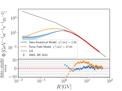
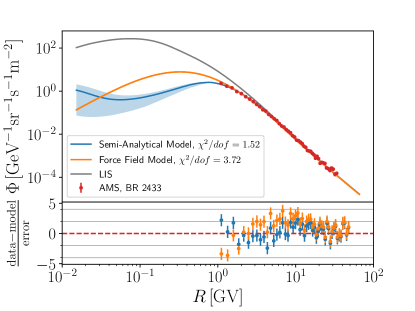
Figure 1: Fit of our semi-analytical model (blue line) to AMS-02 data et al. (2018) and the conventional force-field fit (orange line) for Bartels rotation 2433 for electrons (upper panel) and positrons (lower panel). In both cases the local interstellar spectrum (grey line) is taken from Ref. Vittino et al. (2019). The lower part of the plots shows the pull distribution for the fit. For the blue line the step in the solar wind is fitted while for the blue band it is varied between $\Delta V=0$ and $0.4$.

Prediction of electron-positron fluxes.—While the semi-analytical model with fitted parameters $g_{1}$ and $g_{2}$ for most time intervals nicely reproduces the data, this procedure is not predictive. In order to predict modulated fluxes, we need to model the parameters $g_{1}$ and $g_{2}$ as a function of time. Physically, we would expect them to be (anti-)correlated with solar wind parameters. For example, $g_{1}$ is related to $K_{0}$, which parametrises the strength of diffusion, and could be correlated with a proxy for solar activity, e.g. the tilt angle $\alpha$, while $g_{2}$, which parametrises the relative strength of drifts, could be anti-correlated with the strength of the magnetic field, $B$. We stress that both the tilt angle as measured in the solar corona and the field strength as measured by ACE are relatively local observables whereas the cosmic ray particles spend a finite time in the heliosphere. We would therefore expect the fitted parameters to be affected only with a certain delay and after averaging over time.

We have therefore searched for linear correlations between the $g_{1}$ and $g_{2}$ fitted to AMS-02 data and the tilt angle and magnetic field strength using a moving average of width $\tau$, $\langle\alpha\rangle_{\tau}$ and $\langle B\rangle_{\tau}$. It is generally accepted that particles of different signs ($q$) arrive preferably along different directions in different polarity ($A$) cycles, specifically for $qA>0$ ($qA<0$) particles arrive mostly from the polar (equatorial) direction. Due to the waviness of the current sheet propagation through the equatorial region takes longer than through the polar region and this implies also different delays for $qA>0$ and $qA<0$ with electrons ($q<0$) in an $A>0$ cycle experiencing a similar, large delay as positrons ($q>0$) in an $A<0$ cycle. We therefore allow for different widths $\tau$ for different $qA$.

We find good correlations (Pearson correlation coefficients of $\sim 0.9$) between $g_{1}$ and $\langle\alpha\rangle_{\tau}$ for widths of $\tau=12$ and $39$ Bartels rotations for $qA>0$ and $qA<0$, respectively. For $g_{2}$, we find an anti-correlation ($\sim-0.65$) with $\langle B\rangle_{\tau}$ for widths of $\sim 5$ Bartels rotations. We therefore model the scaling factors as $g_{1}^{\pm}=a_{1}^{\pm}+b_{1}^{\pm}\langle\alpha\rangle_{\tau}$ and $g_{2}^{\pm}=a_{2}^{\pm}+b_{2}^{\pm}\langle B\rangle_{\tau}$. To allow for a smoother transition around the solar maximum we adopt $\tau$’s of $21$ and $30$ Bartels rotations for $qA>0$ and $qA<0$ closer to the solar maximum. We summarise the time ranges and averaging widths adopted in Tbl. 1. The beginning and end of the ranges correspond to regions where the polarity could be determined including an additional delay.

start	end	$\tau_{-}$	$\tau_{+}$	$a_{1}^{-}$	$a_{1}^{+}$	$b_{1}^{-}$	$b_{1}^{+}$	$a_{2}^{-}$	$a_{2}^{+}$	$b_{2}^{-}$	$b_{2}^{+}$
$[\text{BR}]$						$[1/\text{deg}]$				$[1/\mu\text{G}]$
2239	2435	12	39	1.79	-0.32	0.025	0.082	1.50	5.80	-0.441	-1.30
2435	2460	21	30	-2.77	-0.88	0.121	0.071	7.59	7.34	-1.62	-1.57
2460	2485	30	21	5.14	-0.46	0.012	0.068	6.18	5.46	-1.31	-1.16
2485	2530	39	12	0.37	-1.57	0.094	0.107	-0.049	3.95	-0.313	-0.808

Table 1: Interval ranges and averaging widths for electrons ($\tau_{-}$) and positrons ($\tau_{+}$) as well as model coefficients.

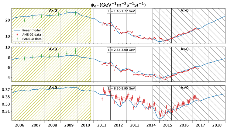
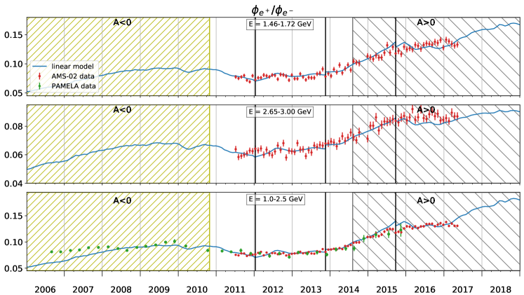
Figure 2: Time-dependent electron flux (upper panels) and positron ratio (lower panels), calculated with our linear model (blue line) and compared to AMS-02 data (red dots). The bottom panel shows an average over multiple bins in order to compare to PAMELA data Munini et al. (2018) (green dots) with wider energy bins. The vertical lines show the transitions between different ranges around the solar maximum. The hatched regions before 2011 and starting in 2014 denote the periods for which the polarity could be unambiguously determined Krainev et al. (2015).

In Fig. 2, we show the electron fluxes and positron-to-electron ratios as a function of time for different energy ranges. There are some deviations from the data that take place on short time scales and are usually coincident with known Forbush decreases that cannot be captured by our model. In order to assess the quality of the fit, one needs to compare against an alternative model for the long term variation. A harmonic fit of the fluxes in each of the $49$ individual energy bins $i$ as $\phi_{i}=A_{i}+B_{i}\cos(2\pi t/T_{i}+\varphi_{i})$ seems as agnostic a model as possible. In this harmonic model with $49\times 4$ free parameters, the $\chi^{2}/\text{dof}$ is $35920/3626$ for electrons and $19447/3626$ for positrons. This is to be compared to $26384/3806$ for electrons and $8028/3806$ for positrons in our model ($4$ time intervals with $4$ parameters each). In the positron ratio the short term features cancel and the $\chi^{2}/\text{dof}=4991/3790$ is much better than for the electron flux or the positron flux alone.

While our model thus reproduces the measurements by AMS-02 rather well, we can predict the fluxes and the ratio also at other times. First, our model can be straight-forwardly extended to earlier times. We note that we also reproduce the measurements of PAMELA even though PAMELA data have not been used in the fitting of the coefficients $a^{\pm}_{1}$, $b^{\pm}_{1}$, $a^{\pm}_{2}$ or $b^{\pm}_{2}$. Second, we can also make a prediction for the fluxes and the ratio for the range for which measurements of $\alpha$ and $B$ are available, in principle until the end of the $A>0$ polarity cycle. As a general trend, we would expect the tilt angle to start rising again soon, leading to a falling positron ratio and subsequent maxima in the positron and electron fluxes.

Conclusion.—We have presented a 2D semi-analytical model that incorporates charge-sign dependent modulation effects due to drifts in the solar magnetic field. We have validated our model by comparing to the results of our finite-difference code and found that the semi-analytical model is significantly more accurate than the conventional force field model. Our model has four free parameters, two of which encode the strength of diffusion and drifts.

It is remarkable that allowing these two free parameters to vary per time interval we can fit the time-dependent AMS-02 electron and positron fluxes rather accurately. Introducing in addition a linear model relating these two parameters to solar wind parameters, we can reproduce not only the AMS-02 measurements, but also the PAMELA electrons fluxes which do not overlap with the AMS-02 electron fluxes. We can also predict the electron and positron fluxes beyond the range for which data has been published. We stress that our method is significantly faster than numerical methods and more accurate than the standard force field model. It can thus be applied to large datasets with fine time binning like the current AMS-02 data. Given its simplicity, it should therefore be applied in phenomenological studies of cosmic ray transport and we facilitate such applications by providing an example script at https://git.rwth-aachen.de/kuhlenmarco/effmod-code.

Acknowledgments.—We are grateful to Henning Gast, Stefan Schael and Andrea Vittino for helpful discussions.

References

- Potgieter [2013] Marius Potgieter. Solar Modulation of Cosmic Rays. Living Rev. Solar Phys., 10:3, 2013. doi: 10.12942/lrsp-2013-3.
- Kappl [2016] Rolf Kappl. Charge-sign dependent solar modulation for everyone. J. Phys. Conf. Ser., 718(5):052020, 2016. doi: 10.1088/1742-6596/718/5/052020.
- Vittino et al. [2018] Andrea Vittino, Carmelo Evoli, and Daniele Gaggero. Cosmic-ray transport in the heliosphere with HelioProp. PoS, ICRC2017:024, 2018. doi: 10.22323/1.301.0024. [35,24(2017)].
- Boschini et al. [2018] M. J. Boschini, S. Della Torre, M. Gervasi, G. La Vacca, and P. G. Rancoita. Propagation of cosmic rays in heliosphere: The HELMOD model. Adv. Space Res., 62(10):2859–2879, Nov 2018. doi: 10.1016/j.asr.2017.04.017.
- Aslam et al. [2019] O. P. M. Aslam, D. Bisschoff, M. S. Potgieter, M. Boezio, and R. Munini. Modeling of Heliospheric Modulation of Cosmic-Ray Positrons in a Very Quiet Heliosphere. ApJ, 873(1):70, Mar 2019. doi: 10.3847/1538-4357/ab05e6.
- Potgieter et al. [2015] M. S. Potgieter, E. E. Vos, R. Munini, M. Boezio, and V. Di Felice. Modulation of Galactic Electrons in the Heliosphere during the Unusual Solar Minimum of 2006-2009: A Modeling Approach. ApJ, 810:141, September 2015. doi: 10.1088/0004-637X/810/2/141.
- Jerome Boschini et al. [2019] Matteo Jerome Boschini, Stefano Della Torre, Massimo Gervasi, Giuseppe La Vacca, and Pier Giorgio Rancoita. The HelMod Model in the Works for Inner and Outer Heliosphere: from AMS to Voyager Probes Observations. arXiv e-prints, art. arXiv:1903.07501, Mar 2019.
- Corti et al. [2019] C. Corti, M. S. Potgieter, V. Bindi, C. Consolandi, C. Light, M. Palermo, and A. Popkow. Numerical Modeling of Galactic Cosmic-Ray Proton and Helium Observed by AMS-02 during the Solar Maximum of Solar Cycle 24. ApJ, 871:253, February 2019. doi: 10.3847/1538-4357/aafac4.
- Gleeson and Axford [1968a] L. J. Gleeson and W. I. Axford. Solar Modulation of Galactic Cosmic Rays. ApJ, 154:1011, December 1968a. doi: 10.1086/149822.
- Cuoco et al. [2019] Alessandro Cuoco, Jan Heisig, Lukas Klamt, Michael Korsmeier, and Michael Krämer. Scrutinizing the evidence for dark matter in cosmic-ray antiprotons. Phys. Rev., D99(10):103014, 2019. doi: 10.1103/PhysRevD.99.103014.
- Cholis et al. [2016] Ilias Cholis, Dan Hooper, and Tim Linden. A Predictive Analytic Model for the Solar Modulation of Cosmic Rays. Phys. Rev., D93(4):043016, 2016. doi: 10.1103/PhysRevD.93.043016.
- Gieseler et al. [2017] Jan Gieseler, Bernd Heber, and Konstantin Herbst. An empirical modification of the force field approach to describe the modulation of galactic cosmic rays close to Earth in a broad range of rigidities. J. Geophys. Res. Space Phys., 122(11):10,964–10,979, 2017. doi: 10.1002/2017JA024763.
- Compton and Getting [1935] Arthur H. Compton and Ivan A. Getting. An Apparent Effect of Galactic Rotation on the Intensity of Cosmic Rays. Physical Review, 47(11):817–821, Jun 1935. doi: 10.1103/PhysRev.47.817.
- Caballero-Lopez and Moraal [2004] R. A. Caballero-Lopez and H. Moraal. Limitations of the force field equation to describe cosmic ray modulation. J. Geophys. Res. Space Phys., 109(A1):A01101, Jan 2004. doi: 10.1029/2003JA010098.
- et al. [2018] M. Aguilar et al. Observation of complex time structures in the cosmic-ray electron and positron fluxes with the alpha magnetic spectrometer on the international space station. Phys. Rev. Lett., 121:051102, Jul 2018. doi: 10.1103/PhysRevLett.121.051102. URL https://link.aps.org/doi/10.1103/PhysRevLett.121.051102.
- Vittino et al. [2019] Andrea Vittino, Philipp Mertsch, Henning Gast, and Stefan Schael. Breaks in interstellar spectra of positrons and electrons derived from time-dependent AMS data. Phys. Rev., D100(4):043007, 2019. doi: 10.1103/PhysRevD.100.043007.
- Munini et al. [2018] R. Munini et al. Ten years of positron and electron solar modulation measured by the PAMELA experiment. PoS, ICRC2017:012, 2018. doi: 10.22323/1.301.0012.
- Krainev et al. [2015] M. Krainev, B. Bazilevskaya, M. Kalinin, A. Svirzhevskaya, and N. Svirzhevsky. GCR intensity during the sunspot maximum phase and the inversion of the heliospheric magnetic field. PoS, 2015. doi: 10.22323/1.236.0081.
- Gleeson and Axford [1968b] L. J. Gleeson and W. I. Axford. The solar radial gradient of galactic cosmic rays. Canadian Journal of Physics Supplement, 46:937, 1968b. doi: 10.1139/p68-388.
- Gleeson and Urch [1971] L. J. Gleeson and I. H. Urch. Energy losses and modulation of galactic cosmic rays. Astrophysics and Space Science, 11(2):288–308, May 1971. doi: 10.1007/BF00661360.
- Webb and Gleeson [1979] G. M. Webb and L. J. Gleeson. On the equation of transport for cosmic-ray particles in the interplanetary region. Astrophysics and Space Science, 60(2):335–351, Feb 1979. ISSN 1572-946X. doi: 10.1007/BF00644337. URL https://doi.org/10.1007/BF00644337.
- Moraal [2013] H. Moraal. Cosmic-Ray Modulation Equations. Space Sci. Rev., 176(1-4):299–319, Jun 2013. doi: 10.1007/s11214-011-9819-3.
- Langner [2004] Ulrich Langner. Effects of Acceleration at the Termination Shock on Cosmic Rays in the Heliosphere. PhD thesis, Northwest University, Potchefstroom, 2004. PhD thesis.
- Teufel and Schlickeiser [2002] A. Teufel and R. Schlickeiser. Analytic calculation of the parallel mean free path of heliospheric cosmic rays. I. Dynamical magnetic slab turbulence and random sweeping slab turbulence. A&A, 393:703–715, October 2002. doi: 10.1051/0004-6361:20021046.
- Burger and Potgieter [1989] R. A. Burger and M. S. Potgieter. The calculation of neutral sheet drift in two-dimensional cosmic-ray modulation models. ApJ, 339:501–511, April 1989. doi: 10.1086/167313.
- Heber and Potgieter [2006] B. Heber and M.S. Potgieter. Cosmic rays at high heliolatitudes. Space Sci. Rev., 127(117), 2006. URL https://doi.org/10.1007/s11214-006-9085-y.
- Burger et al. [2000] R. A. Burger, M. S. Potgieter, and B. Heber. Rigidity dependence of cosmic ray proton latitudinal gradients measured by the Ulysses spacecraft: Implications for the diffusion tensor. J. Geophys. Res., 105:27447–27456, December 2000. doi: 10.1029/2000JA000153.
- Giacalone and Jokipii [1999] J. Giacalone and J. R. Jokipii. The Transport of Cosmic Rays across a Turbulent Magnetic Field. ApJ, 520:204–214, July 1999. doi: 10.1086/307452.