On generating random Gaussian graphical models

Abstract

Structure learning methods for covariance and concentration graphs are often validated on synthetic models, usually obtained by randomly generating: (i) an undirected graph, and (ii) a compatible symmetric positive definite (SPD) matrix. In order to ensure positive definiteness in (ii), a dominant diagonal is usually imposed. In this work we investigate different methods to generate random symmetric positive definite matrices with undirected graphical constraints. We show that if the graph is chordal it is possible to sample uniformly from the set of correlation matrices compatible with the graph, while for general undirected graphs we rely on a partial orthogonalization method.

1 Introduction

Structure learning algorithms in graphical models are validated using either benchmark or randomly generated synthetic models from which data is sampled. This allows to evaluate their performance by comparing the recovered graph, obtained by running the algorithm over the generated data, with the known true structure. The synthetic graphical models are typically constructed in a two-step manner: a graph structure is selected at random or chosen so that it is representative of the problem at hand; and, similarly, its parameters are fixed or randomly sampled.

Covariance (Cox and Wermuth, 1993; Kauermann, 1996) and concentration graphs (Dempster, 1972; Lauritzen, 1996) are graphical models where the variables are assumed to follow a multivariate Gaussian distribution, and the structure is directly read off in the covariance or concentration matrix, respectively. Looking at the literature on these models, one finds that typical benchmark structures are Toeplitz, banded, diagonally spiked and block diagonal covariance or concentration matrices (Yuan and Lin, 2007; Xue and Zou, 2012; Ledoit and Wolf, 2012), with parameters fixed to ensure positive definiteness.

The issue of positive definiteness is especially relevant when the structure is randomly generated. One approach to ensure it is to sample from a matrix distribution with support over the symmetric positive definite matrices compatible with the undirected graph structure. The hyper Wishart distributions (Dawid and Lauritzen, 1993; Letac and Massam, 2007) are the most developed in this context, since they form a conjugate family for Bayesian analysis. However, while sampling algorithms are available for general concentration graphs (Carvalho et al., 2007; Lenkoski, 2013), in covariance graphs they have been developed only in the decomposable case (Khare and Rajaratnam, 2011).

In general, hyper Wishart distributions are rarely used in validation scenarios (Williams et al., 2018), and instead in the literature the most common approach to ensure positive definiteness is to enforce diagonal dominance in the covariance or concentration matrix (Lin et al., 2009; Arvaniti and Claassen, 2014; Stojkovic et al., 2017). However, when the undirected graph is moderately dense, the off-diagonal elements in the generated matrices, often interpreted as link strengths, are extremely small with respect to the diagonal entries and structure recovery becomes a challenge, thereby compromising the structure learning algorithm validation (Schäfer and Strimmer, 2005a, b; Krämer et al., 2009; Cai et al., 2011).

In this paper, we propose alternative methods to generate positive definite matrices with undirected graphical constraints: the partial orthogonalization method proposed in Córdoba et al. (2018), uniform sampling when the graph is chordal and a combination of uniform sampling and partial orthogonalization for general graphs. We show that the partial orthogonalization method could suffer from drawbacks similar to the diagonal dominance when the matrix factor is obtained with i.i.d. elements. For this reason we propose to combine uniform sampling for chordal graphs and the partial orthogonalization method.

We also use our simulation method in a validation setting and show how the performance ranking of the various structure learning algorithms change dramatically, thereby modifying the conclusions drawn if only using diagonally dominant matrices for comparison.

The rest of the paper is organized as follows. Preliminaries are introduced in Section 2, where we briefly overview concentration, covariance graphs and directed graphical models. Next, in Section 3, we present the classical diagonal dominance method, a proposed partial orthogonalization method and the uniform sampling for chordal graphs. Section 4 contains a description of the experiment set-up we have considered, and the interpretation of the results obtained. Finally, in Section 5 we conclude the paper and outline our plans for future research.

2 Preliminaries

In the remainder of the paper, we will use the following notation. We let $X_{1},\ldots,X_{p}$ denote $p$ random variables and $\boldsymbol{X}$ the random vector they form. For each subset $I\subseteq\{1,\ldots,p\}$, $\boldsymbol{X}_{I}$ will be the subvector of $\boldsymbol{X}$ indexed by $I$, that is, $(X_{i})_{i\in I}$. We follow Dawid (1980) and abbreviate conditional independence in the joint distribution of $\boldsymbol{X}$ as $\boldsymbol{X}_{I}\perp\!\!\!\perp\boldsymbol{X}_{J}\mid\boldsymbol{X}_{K}$, meaning that $\boldsymbol{X}_{I}$ is conditionally independent of $\boldsymbol{X}_{J}$ given $\boldsymbol{X}_{K}$, with $I,J,K$ pairwise disjoint subsets of indices. Entries in a matrix are denoted with the respective lower case letter, for example, $m_{ij}$ denotes the $(i,j)$ entry in matrix $\boldsymbol{\mathrm{M}}$.

With $\mathbb{S}$ and $\mathbb{S}^{p}_{>0}$ we denote the sets of symmetric and symmetric positive definite matrices of dimension $p\times p$. We denote the set of symmetric positive definite matrices with unit diagonal as,

$$\mathcal{E}_{p}=\{\boldsymbol{\mathrm{M}}\in\mathbb{S}^{p}_{>0}\text{ s.t. }m_{ii}=1\quad\text{for }i=1,\ldots,p\}.$$

The set $\mathcal{E}_{p}$ is called the elliptope of dimension $p$ (Tropp, 2018) and its volume has been obtained by Joe (2006) and Lewandowski et al. (2009).

With $\mathcal{S}^{k}_{+}$ we denote the $k$-dimensional hemisphere with positive first coordinate,

$$\mathcal{S}^{k}_{+}=\{\boldsymbol{v}\in\mathbb{R}^{k}\text{ s.t. }||\boldsymbol{v}||_{2}=1\text{ and }v_{1}>0\}.$$

We will also use $\mathcal{U}^{p}$ to denote the set of upper triangular matrices of dimension $p\times p$ with positive diagonal, that is, the sets of Cholesky factors for positive definite matrices. With $\mathcal{U}^{p}_{1}\subset\mathcal{U}^{p}$ we denote the subset with unit rows, that is the Cholesky factors for correlation matrices.

2.1 Undirected Gaussian graphical models

Covariance and concentration graphs are graphical models where it is assumed that the statistical independences in the distribution of a multivariate Gaussian random vector $\boldsymbol{X}=(X_{1},\ldots,X_{p})$ can be represented by an undirected graph $G=(V,E)$. Typically, $\boldsymbol{X}$ is assumed to have zero mean for lighter notation, and $V=\{1,\ldots,p\}$ so that it indexes the random vector, that is, $\boldsymbol{X}_{V}=\boldsymbol{X}$. We will represent the edge set $E$ as a subset of $V\times V$, therefore $(i,j)\in E$ if and only if $(j,i)\in E$.

In covariance graphs, the independences represented are marginal, meaning that whenever there is a missing edge $(i,j)$ in $G$, the random variables $X_{i}$ and $X_{j}$ are marginally independent. More formally, this is called the pairwise Markov property of covariance graphs (Cox and Wermuth, 1993; Kauermann, 1996),

$$X_{i}\perp\!\!\!\perp X_{j}\quad\text{for }i,j\in V\text{ s.t. }i\not\sim_{G}j,$$

where $i\sim_{G}j$ is the adjacency relationship on the graph $G$, that is, $i\sim_{G}j$ if and only if $(i,j)\in E$. Note further that $X_{i}\perp\!\!\!\perp X_{j}$ if and only if $\sigma_{ij}=0$.

By contrast, in concentration graphs, a missing edge implies a conditional independence; specifically, in this case the pairwise Markov property (Lauritzen, 1996) becomes

$$X_{i}\perp\!\!\!\perp X_{j}\mid\boldsymbol{X}_{V\setminus\{i,j\}}\quad\text{for }i,j\in V\text{ s.t. }i\not\sim_{G}j.$$

In turn, this can be read off in the concentration matrix $\boldsymbol{\mathrm{\Omega}}=\boldsymbol{\mathrm{\Sigma}}^{-1}$, that is, $X_{i}\perp\!\!\!\perp X_{j}\mid\boldsymbol{X}_{V\setminus\{i,j\}}\iff\omega_{ij}=0$.

Therefore, the statistical independences implied by both covariance and concentration graph models are in correspondence with zero entries in a symmetric positive definite matrix. Thus, in the following we will focus on how to simulate such kind of matrices. For a fixed undirected graph $G$ let ${\mathcal{M}^{p}(G)}$ be the set of matrices with zeros in the entries represented by the missing edges in $G$, that is,

$$\mathcal{M}^{p}(G)=\{\boldsymbol{\mathrm{M}}\in{\mathbb{R}^{p\times p}}:m_{ij}=m_{ji}=0\text{ if }(i,j)\notin E\}.$$

Let $\mathbb{S}^{p}(G)=\mathbb{S}^{p}\cap\mathcal{M}^{p}(G)$ and $\mathbb{S}^{p}_{>0}(G)=\mathbb{S}^{>0}\cap\mathcal{M}^{p}(G)$ be the sets of symmetric and symmetric positive definite matrices with undirected graphical constraints. Similarly $\mathcal{E}_{p}(G)=\mathcal{E}_{p}\cap\mathcal{M}^{p}(G)$ is the set of correlation matrices with undirected graphical constraints.

Note that the covariance matrix $\boldsymbol{\mathrm{\Sigma}}$ of a Gaussian random vector $\boldsymbol{X}$ whose distribution belongs to a covariance graph with structure $G$ satisfies that $\boldsymbol{\mathrm{\Sigma}}\in{\mathbb{S}^{p}_{>0}(G)}$. Analogously, if the distribution belongs to a concentration graph with structure $G$, then $\boldsymbol{\mathrm{\Omega}}=\boldsymbol{\mathrm{\Sigma}}^{-1}\in{\mathbb{S}^{p}_{>0}(G)}$. In either case it is clear that the goal is to simulate elements belonging to $\mathbb{S}^{p}_{>0}(G)$, or to $\mathcal{E}^{p}(G)$.

2.2 Cholesky factorization and directed graphical models

If $G=(V=\{1,\ldots,p\},E)$ is an acyclic directed graph and we assume that $1\prec\cdots\prec p$ is a topological order, that is, $\operatorname{pa}(i)\subseteq\{1,\ldots,i-1\}$ for all $i\in V$, then we can define the ordered Markov property for the Bayesian network model,

$$X_{i}\perp\!\!\!\perp X_{j}|\boldsymbol{X}_{\operatorname{pa}({i})}\quad\text{for all }i\in V,\,{j}\not\in\operatorname{pa}({i}),\,j{<}i.$$ (1)

If the ordered Markov property holds for a Gaussian distribution it is equivalent to saying that the coefficient $\beta_{ij}$ of variable $X_{j}$ in the regression of $X_{i}$ on $X_{1},\ldots,X_{{i}-1}$ is zero for all $j\notin\operatorname{pa}(i)$. Therefore, the set of edges $E$ in a Gaussian Bayesian network can be expressed as

$$E=\{(j,i)\text{ s.t. }\beta_{ij}\neq 0\},$$ (2)

We can rewrite the above Markov property as a triangular regression system (Wermuth, 1980). Specifically, for each $i\in V$, $X_{i}$ can be written as a regression over its parents,

$$X_{i}=\sum_{j<i}\beta_{ij}X_{j}+\varepsilon_{i}=\sum_{j\in\operatorname{pa}(i)}\beta_{ij}X_{j}+\varepsilon_{i},$$ (3)

where $\varepsilon_{1},\ldots,\varepsilon_{p}$ is a vector of zero-mean independent Gaussian noise.

We can write Equation (3) in matrix notation as $\boldsymbol{X}=\boldsymbol{\mathrm{B}}\boldsymbol{X}+\boldsymbol{\varepsilon}$, with $\boldsymbol{\mathrm{B}}$ strictly lower triangular, since $1,\ldots,p$ is assumed to be a topological order of $G$. Rearranging the equation we obtain $\boldsymbol{X}=(\boldsymbol{\mathrm{I}}_{p}-\boldsymbol{\mathrm{B}})^{-1}\boldsymbol{\varepsilon}$. Taking variances on both sides, we arrive at the upper Cholesky factorization of the precision matrix (Pourahmadi, 1999)

$$\boldsymbol{\mathrm{\Sigma}}^{-1}=\boldsymbol{\mathrm{\Omega}}=(\boldsymbol{\mathrm{I}}_{p}-\boldsymbol{\mathrm{B}})^{t}\boldsymbol{\mathrm{V}}^{-1}(\boldsymbol{\mathrm{I}}_{p}-\boldsymbol{\mathrm{B}})=\boldsymbol{\mathrm{U}}\boldsymbol{\mathrm{U}}^{t},$$ (4)

where $\boldsymbol{\mathrm{U}}=(\boldsymbol{\mathrm{I}}_{p}-\boldsymbol{\mathrm{B}})^{t}\sqrt{\boldsymbol{\mathrm{V}}^{-1}}\in\mathcal{U}^{p}$ and $\boldsymbol{\mathrm{V}}$ is a diagonal matrix with $v_{ii}=\operatorname{var}(\varepsilon_{i}){=\operatorname{var}(X_{i}|\boldsymbol{X}_{\operatorname{pa}(i)})}$.

The upper Cholesky factorization in Equation (4) is closely related to the classical/lower Cholesky factorization, as follows. Let $\tilde{\boldsymbol{\mathrm{\Omega}}}$ be the matrix obtained from $\boldsymbol{\mathrm{\Omega}}$ by reordering the variables so that they follow the reverse of a perfect/topological ordering, also known as fill-in free or perfect elimination ordering (see Roverato, 2000, for example). Then if $\tilde{\boldsymbol{\mathrm{\Omega}}}=\boldsymbol{\mathrm{L}}\boldsymbol{\mathrm{L}}^{t}$ is its standard lower Cholesky decomposition, it can be verified that $\boldsymbol{\mathrm{L}}^{t}$ is equal to the transpose of $\boldsymbol{\mathrm{U}}$ (Equation 4) with respect to its anti-diagonal. Furthermore, the parameters of the Gaussian Bayesian network are obtained from $\boldsymbol{\mathrm{U}}$ (Wermuth et al., 2006) as

$$\beta_{ij}={-}\frac{u_{ji}}{u_{ii}};\hskip 28.45274pt\operatorname{var}(X_{i}|\boldsymbol{X}_{\operatorname{pa}(i)})=\frac{1}{u_{ii}^{2}}.$$ (5)

The upper Cholesky factorization in Equation (4) can be used as a parametrization of the inverse covariance matrix for Gaussian distributions satisfying the ordered Markov property, that is, Gaussian Bayesian networks: from Equation (5) we have that, for $j{<}i$,

$$(j,i)\not\in E\iff X_{i}\perp\!\!\!\perp X_{j}|\boldsymbol{X}_{\operatorname{pa}({i})}\iff\beta_{ij}=0\iff u_{ji}=0,$$ (6)

The Gaussian Bayesian network model can thus be expressed as

$$\mathcal{B}(G)=\{\boldsymbol{\mathrm{\Omega}}=\boldsymbol{\mathrm{\Sigma}}^{-1}=\boldsymbol{\mathrm{U}}\boldsymbol{\mathrm{U}}^{t}\text{ s.t. }\boldsymbol{\mathrm{U}}\in\mathcal{U}^{p}\text{ and }u_{ji}=0\text{ if }(j,i)\notin E\},$$ (7)

where $G=(V,E)$ is an acyclic digraph with $1{\prec\cdots\prec}p$ being a topological order of $G$.

2.3 Markov equivalence between Gaussian graphical models

The intersection between Markov and Bayesian network models occurs at what are called decomposable/chordal/triangulated undirected graphs, or, equivalently, acyclic digraphs with no v-structures. An undirected graph $G$ is said to be chordal if all cycles of length at least 4 have a chord. A v-structure in an acyclic digraph $G$ with edge set $E$, is a configuration where if $(i,j)\in E$, $(k,j)\in E$ and $i\neq k$, then $(i,k)\notin E$ and $(k,i)\notin E$, that is, a v-structure is when two vertices share a common child but they are not adjacent. If an acyclic digraph has no v-structures, then for each node the set of parents is completely connected. The skeleton of an acyclic digraph with no v-structures is chordal; and, equivalently, any chordal undirected graph can be oriented into an acyclic digraph with no v-structures, as follows: let $C_{1},\ldots,C_{k}$ denote a perfect sequence of cliques in an undirected chordal graph $G=(V,E)$, and write $H_{j}=C_{1}\cup\ldots\cup C_{j}$, $R_{j}=C_{j}\setminus H_{j-1}$, following Lauritzen (1996). A perfect ordering, $v_{1}\prec\cdots\prec v_{p}$, for the vertices of $G$ is formed by first taking the vertices in ${C}_{1}$, then those in $R_{2}$, until $R_{k}$. This ordering has associated an acyclic directed orientation of $G$, $G_{D}=(V,E_{D})$, which has no v-structures. In fact, $v_{1}\prec\cdots\prec v_{p}$ is a topological ordering for $G_{D}$. Therefore, denoting for $v_{i}\in V$ as $\operatorname{pr}(v_{i})=\{v_{1},\ldots,v_{{i-1}}\}$ and $\operatorname{bd}(v_{i})=\{v_{j}\in V:(v_{i},v_{j})\in E\}$, then we have

$$|E|=\sum_{i=1}^{p}|\operatorname{bd}(v_{i})\cap\operatorname{pr}(v_{i})|=\sum_{i=1}^{p}|\operatorname{pa}(v_{i})|=|E_{D}|.$$

In the Gaussian case, this implies that if $1\prec\cdots\prec p$ is a perfect ordering for $G$. Therefore, the theory of Section 2.2 for Gaussian Bayesian networks applies and $\boldsymbol{\mathrm{\Sigma}}^{-1}=\boldsymbol{\mathrm{U}}\boldsymbol{\mathrm{U}}^{t}$ with $\boldsymbol{\mathrm{U}}\in\mathcal{U}^{p}$ and the same zero pattern as in the upper triangle of $\boldsymbol{\mathrm{\Omega}}=\boldsymbol{\mathrm{\Sigma}}^{-1}$,

$$(j,i)\notin E_{D}\iff u_{ji}=0\iff\omega_{ji}=\omega_{ij}=0\iff(i,j)\notin E.$$ (8)

Thus we have that if $G$ is a chordal undirected graph, then $\mathbb{S}_{>{0}}^{p}(G)=\mathcal{B}(G_{D})$ (Wermuth, 1980; Paulsen et al., 1989).

3 Methods

3.1 Diagonal dominance

When a matrix $\boldsymbol{\mathrm{M}}\in\mathbb{S}^{p}$ satisfies that $m_{ii}>\sum_{j\neq i}|m_{ij}|$ for each $i\in\{1,\ldots,p\}$, then $\boldsymbol{\mathrm{M}}$ belongs to $\mathbb{S}^{p}_{>0}$. Thus a simple method to generate a matrix in $\mathbb{S}^{p}_{>0}(G)$ consists in generating a random matrix in $\mathbb{S}^{p}(G)$ and then choosing diagonal elements so the final matrix is diagonally dominant, as in Algorithm 1. The usual approach for generating the initial matrix in line 1 is to use independent and identically distributed (i.i.d.) nonzero entries. The diagonal dominance method has been extensively used in the literature mainly due to its simplicity and the ability to control the singularity of the generated matrices, as we will now explain.

Algorithm 1 Simulation of a matrix in $\mathbb{S}^{p}_{>0}(G)$ using diagonal dominance

0:  Undirected graph $G$

0:  Matrix belonging to $\mathbb{S}^{p}_{>0}(G)$

1:  $\boldsymbol{\mathrm{M}}\leftarrow$ random matrix in $\mathbb{S}^{p}(G)$

2:  for $i=1,\ldots,p$ do

3:     $m_{ii}\leftarrow\sum_{i\neq j}|{m_{ij}}|+$ random positive perturbation

4:  end for

5:  return  $\boldsymbol{\mathrm{M}}$

Obviously it is then possible to generate correlation matrices in $\mathbb{S}^{p}_{>0}(G)$ using Algorithm 1 and then rescaling them to be in $\mathcal{E}^{p}(G)$.

It is even possible to control the minimum eigenvalue of a matrix by varying its diagonal elements (Honorio et al., 2012). In particular, let $G$ be an undirected graph, $\boldsymbol{\mathrm{M}}$ a matrix in $\mathbb{S}^{p}(G)$, and $\epsilon>0$ the desired lower-bound on the eigenvalues. If $\lambda_{min}$ is the minimum eigenvalue of $\boldsymbol{\mathrm{M}}$, then $\boldsymbol{\mathrm{M}}+(\lambda_{min}^{-}+\epsilon)\boldsymbol{\mathrm{I}}_{p}$ belongs to $\mathbb{S}^{p}_{>0}(G)$ and has eigenvalues greater or equal to $\epsilon$, where $\lambda_{min}^{-}=\max\left(-\lambda_{min},0\right)$ denotes the negative part of $\lambda_{min}$.

Similarly, one can control the condition number, that is, the ratio of the largest to smallest eigenvalue, of the generated matrix as in (Cai et al., 2011): if $\kappa_{0}>1$ is the desired condition number and we already have a matrix $\boldsymbol{\mathrm{M}}\in{\mathbb{S}^{p}(G)}$ with maximum eigenvalue $\lambda_{max}>0$, then

$$\boldsymbol{\mathrm{M}}+\frac{\lambda_{max}-\kappa_{0}\lambda_{min}}{\kappa_{0}-1}\boldsymbol{\mathrm{I}}_{p}$$

belongs to $\mathbb{S}^{p}_{>0}(G)$ and has condition number equal to $\kappa_{0}$. Covariance and concentration matrices with an upper bound on the condition number are appealing in certain estimation scenarios (Joong-Ho et al., 2013).

3.2 Partial orthogonalization

If we consider a full rank matrix $\mathbf{Q}\in\mathbb{R}^{p\times p}$ the product $\mathbf{Q}\mathbf{Q}^{t}$ is a symmetric positive definite matrix. Moreover, $\mathbf{Q}\mathbf{Q}^{t}\in\mathbb{S}^{p}_{>0}(G)$, for a given undirected graph $G$, if and only if:

$$\boldsymbol{q}_{i}\perp\boldsymbol{q}_{j}\quad\text{for }i\not\sim_{G}j{,}$$

where $\bot$ denotes orthogonality with respect to the standard scalar product on $\mathbb{R}^{p}$, and $\boldsymbol{q}_{i}$ is the $i$-th row of $\boldsymbol{\mathrm{Q}}$.

This fact suggests a very simple idea to generate matrices in $\mathbb{S}^{p}_{>0}(G)$: given an undirected graph $G$, we can impose Markov properties for the matrix $\boldsymbol{\mathrm{Q}}\boldsymbol{\mathrm{Q}}^{t}$ simply by orthogonalizing the respective rows of $\boldsymbol{\mathrm{Q}}$. If moreover we also normalize the rows of $\boldsymbol{\mathrm{Q}}$ we generate a matrix in the elliptope with graphical constrains $\mathcal{E}^{p}(G)$. The pseudocode for the described procedure can be found in Algorithm 2.

Algorithm 2 Simulation of a matrix in $\mathcal{E}^{p}(G)$ using partial orthogonalization

0:  Undirected graph $G$

0:  Matrix belonging to $\mathcal{E}^{p}(G)$

1:  $\boldsymbol{\mathrm{Q}}\leftarrow$ random $p\times p$ matrix

2:  for $i=1,\ldots,p$ do

3:     orthogonalize $\boldsymbol{q}_{i}$ with respect to the span of $\{\boldsymbol{q}_{j}\text{ s.t. }i\not\sim_{G}j\text{ and }j<i\}$

4:     normalize $\boldsymbol{q}_{i}$, $\boldsymbol{q}_{i}=\boldsymbol{q}_{i}{/}\lVert\boldsymbol{q}_{i}\rVert_{2}$

5:  end for

6:  return  $\boldsymbol{\mathrm{Q}}\boldsymbol{\mathrm{Q}}^{t}$

In particular we can use a modified Gram-Schmidt orthogonalization procedure that iteratively orthogonalizes every row $\boldsymbol{q}_{i}$ with respect to the set of rows $i^{\bot}=\{\boldsymbol{q}_{j}\text{ s.t. }i\not\sim_{G}j\text{ and }j<i\}$.

3.3 Uniform sampling for chordal graphs

When $G$ is a chordal graph, it is possible to sample uniformly from the set $\mathcal{E}^{p}(G)$ extending the results in Córdoba et al. (2018). In particular, for an undirected chordal graph $G$ where $1\prec\cdots\prec p$ is a perfect ordering, we consider the parametrization of $\mathcal{E}^{p}(G)$ induced by the Cholesky factorization (Section 2.3),

$$\mathcal{E}^{p}(G)=\{\boldsymbol{\mathrm{M}}=\boldsymbol{\mathrm{U}}\boldsymbol{\mathrm{U}}^{t}\text{ s.t. }\boldsymbol{\mathrm{U}}\in\mathcal{U}^{p}_{1}\text{ and }u_{ij}=0\text{ if }(i,j)\not\in E\}.$$

Thus, if we further define the set,

$$\mathcal{U}^{p}_{1}(G)=\{\boldsymbol{\mathrm{U}}\in\mathcal{U}_{1}^{p}\text{ s.t. }u_{ij}=0\text{ if }(i,j)\not\in E\},$$

then

$$\begin{array}[]{lclc}\Phi:&\mathcal{U}^{p}_{1}(G)&\to&\mathcal{E}^{p}(G)\\ &\boldsymbol{\mathrm{U}}&{\mapsto}&\boldsymbol{\mathrm{U}}\boldsymbol{\mathrm{U}}^{t}\end{array}$$

is a one-to-one parametrization of $\mathcal{E}^{p}(G)$. The Jacobian of $\Phi$ has been obtained by Roverato (2000) and in Córdoba et al. (2018), as

$$\det{(J\Phi(\boldsymbol{\mathrm{U}}))}=2^{p}\prod_{i=1}^{p}u_{ii}^{\operatorname{pa}(i)+1}$$ (9)

where $\operatorname{pa}(i)$ denotes the set of parents of node $i$ in $G_{D}$, the acyclic directed orientation of $G$ (which has $1\prec\cdots\prec p$ as a topological ordering, see Section 2.3).

To sample from the uniform distribution over $\mathcal{E}^{p}(G)$ using parametrization $\Phi$, we apply the area formula as Diaconis et al. (2013), Theorem 1: we sample matrices in $\mathcal{U}_{1}^{p}(G)$ from a density proportional to $\det{(J\Phi(\boldsymbol{\mathrm{U}}))}$ and then we apply the parametrization $\Phi$. We observe that the Jacobian of $\Phi$ in Equation (9) factorizes across the rows $\boldsymbol{u}_{i}$ of $\boldsymbol{\mathrm{U}}$, and thus we can sample the rows of $\boldsymbol{\mathrm{U}}$ independently. In particular, for the $i$-th row of $\boldsymbol{\mathrm{U}}$, we have that

$$u_{ij} =0\quad j<i,$$

$$u_{ii} >0,$$

$$u_{ik} =0\quad k\not\in\operatorname{ch}(i),$$

where $\operatorname{ch}(i)$ denotes the children set of node $i$ in graph $G_{D}$. Therefore, for each $i\in\{1,\ldots,p\}$, the vector of non-zero entries in the $i$-th row of $\boldsymbol{\mathrm{U}}$ has to be sampled in the hemisphere $\mathcal{S}_{+}^{|\operatorname{ch}(i)|}$ from a density proportional to a power of the first non-zero entry in such row, $u_{ii}$. This task can be done with the same Metropolis sampling procedure described in detail in Córdoba et al. (2018) and outlined in Algorithm 4 for completeness (with default noise variance $\sigma_{\epsilon}$ and burn-in time $t_{b}$).

Algorithm 3 Uniform sampling in $\mathcal{E}^{p}(G)$

0:  Chordal graph $G$ with $1\prec\cdots\prec p$ as a perfect ordering

0:  A matrix uniformly sampled in $\mathcal{E}^{p}(G)$

1:  $G_{D}\leftarrow$ acyclic directed orientation of $G$

2:  $\boldsymbol{\mathrm{U}}^{n}\leftarrow\boldsymbol{\mathrm{0}}_{p}$

3:  for $i\in\{1,\ldots,p\}$ do

4:     $\boldsymbol{v}\leftarrow{\texttt{mh\_u}(\alpha=|\operatorname{ch}(i)|,\gamma=|\operatorname{pa}(i)|+1)}$

5:     $u_{ii}\leftarrow v_{1}$

6:     $\boldsymbol{u}_{i\operatorname{ch}(i)}\leftarrow\boldsymbol{v}_{-1}$ // Vector $v$ except its first entry

7:  end for

8:  return  $\Phi(\boldsymbol{\mathrm{U}})=\boldsymbol{\mathrm{U}}\boldsymbol{\mathrm{U}}^{t}$

Algorithm 4 mh_u: Metropolis sampling of a vector $\boldsymbol{v}$ in $\mathcal{S}_{+}^{\alpha}$ from $f(\boldsymbol{v})\propto v_{1}^{\gamma}$

0:  Dimension $\alpha$ of the sphere and power $\gamma$ of the density

0:  A vector sampled in $\mathcal{S}_{+}^{\alpha}$

1:  $\boldsymbol{v}_{0}\leftarrow$ random standard multivariate Gaussian observation of dimension $\alpha+1$

2:  $v_{01}\leftarrow|v_{01}|$

3:  $\boldsymbol{v}_{0}\leftarrow$ normalize $\boldsymbol{v}_{0}$

4:  for $t=0,\ldots,t_{b}+1$ do

5:     for $j=1,\ldots,\alpha+1$ do

6:        $\epsilon_{j}\leftarrow$ random Gaussian observation with zero mean and variance $\sigma_{\epsilon}^{2}$

7:     end for

8:     $\boldsymbol{v}^{\prime}\leftarrow\boldsymbol{v}_{t}+\boldsymbol{\epsilon}$

9:     $\boldsymbol{v}^{\prime}\leftarrow$ normalize $\boldsymbol{v}^{\prime}$, $\boldsymbol{v}^{\prime}=\boldsymbol{v}^{\prime}/\lVert\boldsymbol{v}^{\prime}\rVert_{2}$

10:     $\delta\leftarrow$ random uniform observation on $[0,1]$

11:     if $v^{\prime}_{1}\geq 0$ and $\delta\leq(v^{\prime}_{1}/v_{t1})^{\gamma}$ then

12:        $\boldsymbol{v}_{t}\leftarrow\boldsymbol{v}^{\prime}$

13:     end if

14:  end for

15:  return  $\boldsymbol{v}_{t_{b}+1}$

3.4 Combining uniform sampling and partial orthogonalization

When the undirected graph $G$ is not chordal it is not possible to direct the edges without creating v-structures. This implies that applying Algorithm 3 to a triangulation of a non-chordal graph $G$ will result in a matrix with more non-zeros entries than the desired ones. To overcome such issue we propose to combine the two approaches in the previous sections and first sample the Cholesky factor as in Algorithm 3 for the triangulated graph, and then apply the partial orthogonalization procedure as in Algorithm 2 to obtain a matrix in $\mathcal{E}^{p}(G)$.

The method is detailed in Algorithm 5.

Algorithm 5 Simulation of a matrix in $\mathcal{E}^{p}(G)$ combining uniform sampling with respect to a triangulation and partial orthogonalization

0:  Undirected graph $G$

0:  Matrix belonging to $\mathcal{E}^{p}(G)$

1:  $G^{\prime}\leftarrow$ triangulation of $G$ following a perfect ordering defined by permutation $\sigma$

2:  $G_{D}\leftarrow$ acyclic directed orientation of $G^{\prime}$

3:  $\boldsymbol{\mathrm{U}}\leftarrow\boldsymbol{\mathrm{0}}$

4:  for $i=1,\ldots,p$ do

5:     $\boldsymbol{v}\leftarrow{\texttt{mh\_u}(\alpha=|\operatorname{ch}(\sigma(i))|,\gamma=|\operatorname{pa}(\sigma(i))|+1)}$

6:     $u_{ii}\leftarrow v_{1}$

7:     $\boldsymbol{u}_{i\operatorname{ch}(\sigma(i))}\leftarrow\boldsymbol{v}_{-1}$ // Vector $v$ except its first entry

8:  end for

9:  $\boldsymbol{\mathrm{Q}}\leftarrow$ permute rows and columns in $\boldsymbol{\mathrm{U}}$ with $\sigma^{-1}$ // Revert the perfect ordering to retrieve original ordering of the nodes in $G$

10:  for $i=1,\ldots,p$ do

11:     orthogonalize $\boldsymbol{q}_{i}$ with respect to the span of $\{\boldsymbol{q}_{j}\text{ s.t. }i\not\sim_{G}j\text{ and }j<i\}$

12:     normalize $\boldsymbol{q}_{i}$, $\boldsymbol{q}_{i}=\boldsymbol{q}_{i}{/}\lVert\boldsymbol{q}_{i}\rVert_{2}$

13:  end for

14:  return  $\boldsymbol{\mathrm{Q}}\boldsymbol{\mathrm{Q}}^{t}$

For chordal graphs, Algorithm 5 obviously reduces to the uniform sampling of Algorithm 3.

4 Experiments

In this section we report the results of numerical experiments performed to explore the behaviour of the methods presented. The implementation of the methods in the previous sections can be found in the R package gmat. The partial orthogonalization procedure has been implemented in C for improved performance. The experiments can be reproduced following the instructions and using the code available at the repository https://github.com/irenecrsn/ggmsim.

4.1 Three variables

We consider the simple chordal graph $G=(\{1,2,3\},\{\{1,2\},\{2,3\}\})$ over three variables depicted in Figure 1, and we analyze graphically how the three proposed methods behave.

Figure 1: Chordal undirected graph with three variables.

We sample $5000$ correlation matrices from $\mathcal{E}^{3}(G)$ using the diagonal dominance method (Algorithm 1), the partial orthogonalization method (Algorithm 2) and the uniform sampling (Algorithm 3). We use independent standard Gaussian random variables to initialize the random matrices in both Algorithms 1 and 2. Matrices in $\mathcal{E}^{3}(G)$ have two non-zero upper triangular entries $(1,2)$ and $(2,3)$, and moreover $\mathcal{E}^{3}(G)$ can be represented as the interior of the two dimensional unit ball:

$$\mathcal{E}^{3}(G)=\left\{\left(\begin{matrix}1&x&0\\ x&1&y\\ 0&y&1\end{matrix}\right)\text{ s.t. }x^{2}+y^{2}<1\right\}\simeq\{(x,y)\in\mathbb{R}^{2}\text{ s.t. }x^{2}+y^{2}<1\}$$

The scatter plot of the two non-zero upper triangular entries for the three sampling methods is shown in Figure 2

Figure 2: Scatter plot of the two non-zero entries for correlation matrices sampled from $\mathcal{E}^{3}(G)$, with $G$ as in Figure 1.

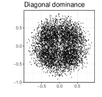
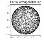
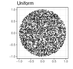
We can see that, as expected, the uniform sampling method obtains a uniform distribution over $\mathcal{E}^{3}(G)$ while the diagonal dominance method and the partial orthogonalization methods have somehow the opposite behaviour. Matrices sampled with partial orthogonalization tend to have large off-diagonal values, while the diagonal dominance method produces matrices with smaller values for the off-diagonal entries.

4.2 Marginal distribution of matrix entries

We investigate here the marginal distribution of non-zeros matrix entries sampled from $\mathcal{E}^{p}(G)$ with the different methods, for both chordal and non-chordal graphs.

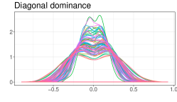
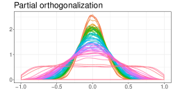
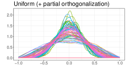
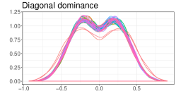
We generate a random undirected graph $G$ over $50$ vertices using the Erdős-Rényi model with a probability of edges equal to $0.05$. We sample $5000$ matrices from $\mathcal{E}^{50}(G)$ using Algorithms 1, 2 and 5. We then plot the marginal densities of the non-zero entries for the three methods. The results are shown in Figure 3.

Figure 3: Marginal densities of the non-zero entries of matrices sampled from $\mathcal{E}^{50}(G)$; where $G$ is a random graph with $50$ vertices and probability of edges $0.05$. The first entry in the lower triangle (2, 1) corresponds to the red colour, while the last entry in the last row of the lower triangle (50, 49) corresponds to the pink colour.

We also consider $G^{\prime}$, the triangulation of $G$ and we generate again $5000$ matrices in $\mathcal{E}^{50}(G^{\prime})$ using the three methods. Plots of the marginal densities of the non-zero entries are shown in Figure 4.

Figure 4: Marginal densities of the non-zero entries of matrices sampled from $\mathcal{E}^{50}(G^{\prime})$; where $G^{\prime}$ is the chordal graphs obtained as the triangulation of a random graph with $50$ vertices and probability of edges $0.05$. The first entry in the lower triangle (2, 1) corresponds to the red colour, while the last entry in the last row of the lower triangle (50, 49) corresponds to the pink colour.

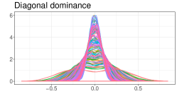
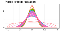
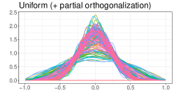
From both Figures 3 and 4 we can observe that the diagonal dominance method produces matrices with off-diagonal entries more concentrated around $0$, as also pointed-out in Córdoba et al. (2018). In apparent contrast to the finding in Córdoba et al. (2018), also the partial orthogonalization method seems to produce matrices with entries more concentrated around $0$. Intuitively this can be seen as a consequence of the fact that vectors of independent random components are approximately orthogonal in high-dimensions. To further prove this problem of the partial orthogonalization algorithm, we simulate $5000$ matrices from $\mathcal{E}^{50}(G_{chain})$, where $G_{chain}=\left(\{1,\ldots,50\},\{\{1,2\},\{2,3\},\ldots,\{49,50\}\}\right)$ (see Figure 5).

Figure 5: Chordal undirected graph $G_{chain}$ with 50 variables and 49 edges

As usual we plot the marginal densities of the $49$ non-zero entries of the generated matrices with the three different methods ($G_{chain}$ is chordal and thus we can sample uniformly) (see Figure 6).

Figure 6: Marginal densities of the non-zero entries of matrices sampled from $\mathcal{E}^{50}(G_{chain})$. The first entry in the lower triangle, (2, 1), corresponds to the red colour, while the last entry in the last row of the lower triangle, (49, 48), corresponds to the pink colour.

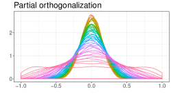
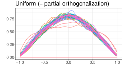
We observe that for this graph the distribution induced on the matrix entries is completely different for the three methods. In particular it is interesting to note that the partial orthogonalization method produces matrices $\boldsymbol{\mathrm{M}}\in\mathcal{E}^{50}(G_{chain})$ with the first non-zero entries $m_{1,2},m_{2,3},m_{3,4},\ldots$ more centered around $0$ than the last entries $\ldots,m_{48,49},m_{49,50}$. On the contrary the uniform sampling, correctly produces matrices with the same marginal densities for the entries. This behaviour of the partial orthogonalization procedure is due to the i.i.d. sampling of the elements of factor $\boldsymbol{\mathrm{Q}}$ in Algorithm 2 and not to the orthogonalization part, that instead mitigates this fact (the first entries of the matrix $m_{1,2},m_{2,3}$ are the ones where no-orthogonalization is applied by Algorithm 2). We remark that such problem for the partial orthogonalization procedure applied to a random matrix $\boldsymbol{\mathrm{Q}}$ with i.i.d. entries can be disturbing since it introduces some asymmetries in the distribution of the matrices that are absent in graph $G$.

4.3 Validation of structure learning algorithms

The main motivation for the proposed method are the observations that can be found in the literature on covariance and concentration graphs regarding the difficulties of validating the performance of structure learning algorithms (Schäfer and Strimmer, 2005a; Krämer et al., 2009; Cai et al., 2011). In particular, Krämer et al. (2009) obtain significantly poorer graph recovery results as the density of the graphs grows. They simulate the corresponding concentration graph models using the diagonal dominance method, so we have replicated their experiments but using instead as true models those generated with our proposed method. The results can be seen in Figures 7 and 8, where we have plotted the true positive rate (also called power by Krämer et al. (2009)) and discovery rates for $p=100$ and their sparsest ($d=0.05$) and densest ($d=0.25$) scenarios, using matrices simulated with the diagonal dominance (Algorithm 1) and our proposed method (Algorithm 5). The different structure learning methods are the same than those studied by Krämer et al. (2009).

Figure 7: True positive rate (TPR) and true discovery rate (PPV) of the structure learning algorithms for concentration graphs validated in (Krämer et al., 2009), for the highest density, 0.25. The number of variables (vertices in the undirected graph and dimension of the generated matrices) is fixed at $100$. adalasso: Adaptive $l_{1}$ regularization; lasso: $l_{1}$ regularization; pls: partial least squares regression; shrink: shrinkage estimator of Schäfer and Strimmer (2005b); ridge: $l_{2}$ regularization; diagdom: Diagonal dominance sampling method; port_chol: Uniform sampling with partial orthogonalization of the Cholesky factor.

Figure 8: True positive rate (TPR) and true discovery rate (PPV) of the structure learning algorithms for concentration graphs validated in (Krämer et al., 2009), for the lowest density, 0.05. The number of variables (vertices in the undirected graph and dimension of the generated matrices) is fixed at $100$. adalasso: Adaptive $l_{1}$ regularization; lasso: $l_{1}$ regularization; pls: partial least squares regression; shrink: shrinkage estimator of Schäfer and Strimmer (2005b); ridge: $l_{2}$ regularization; diagdom: Diagonal dominance sampling method; port_chol: Uniform sampling with partial orthogonalization of the Cholesky factor.

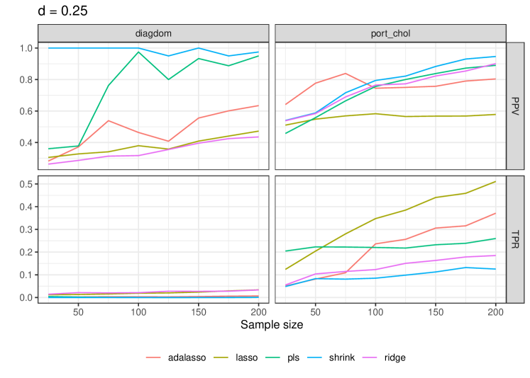
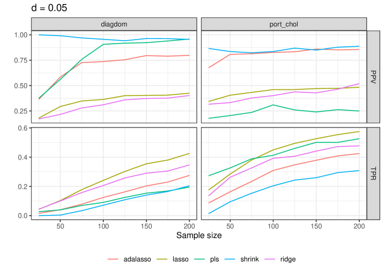
Note that there is a significant improvement in the densest ($d=0.5$) when using our method (Algorithm 5). All the learning algorithms are close to zero true positive rate for every sample size when validating on diagonally dominant matrices, which highlights a poor performance (the high true discovery rates are thus not significant). However, when using matrices obtained via partial orthogonalization, some methods are able to achieve a true positive rate (lasso) of $0.5$ approximately. Importantly, partial least squares regression (pls) and the shrinkage estimator (shrink) greatly improve, whereas when only using diagonal dominance one could erroneously conclude that those methods are not well fitted for dense structure scenarios.

In the sparsest scenario ($d=0.05$) we observe that the partial least square algorithm performs extremely badly when using our proposed method with respect to the true discovery rate, while the other algorithms rank similarly using diagonal dominance or uniform sampling plus partial orthogonalization. This small real example already serves to highlight the practical application and usefulness of our proposed method, and moreover we observe that the sampling procedure highly influence how the structure learning algorithms are ranked.

5 Conclusions

In this work we introduced two methods to sample from the set $\mathcal{E}^{p}(G)$ of correlation matrices with undirected graphical constraints, a general partial orthogonalization procedure and a uniform sampling method when the graph $G$ is chordal. We showed with some numerical experiments that both the partial orthogonalization method and the classical diagonal dominance procedure suffer from some drawbacks in effectively exploring the space of correlation matrices with undirected graphical constraints. For chordal graphs, it is possible to sample from the uniform distribution easily, extending a method to sample correlation matrices uniformly; while for non-chordal graphs we propose to combine the uniform sampling method and the partial orthogonalization by firstly sampling a Cholesky factor related to the triangulated graph and then applying the partial orthogonalization to remove the non-zeros entries related to the edges added in the triangulation. The proposed method has shown to be helpful in the validation of structure learning algorithms overcoming the problems of the diagonal dominance method. The main direction for future research is to investigate how to sample uniformly form the space $\mathcal{E}^{p}(G)$ for a non-chordal graph $G$.

References

- Arvaniti and Claassen (2014) Arvaniti, E., Claassen, M., 2014. Markov network structure learning via ensemble-of-forests models, in: Proceedings of the Thirtieth Conference on Uncertainty in Artificial Intelligence, AUAI Press. pp. 42–51.
- Cai et al. (2011) Cai, T., Liu, W., Luo, X., 2011. A constrained minimization approach to sparse precision matrix estimation. Journal of the American Statistical Association 106, 594–607.
- Carvalho et al. (2007) Carvalho, C.M., Massam, H., West, M., 2007. Simulation of hyper-inverse Wishart distributions in graphical models. Biometrika 94, 647–659.
- Córdoba et al. (2018) Córdoba, I., Varando, G., Bielza, C., Larrañaga, P., 2018. A partial orthogonalization method for simulating covariance and concentration graph matrices, in: Kratochvíl, V., Studený, M. (Eds.), Proceedings of the Ninth International Conference on Probabilistic Graphical Models, PMLR, Prague, Czech Republic. pp. 61–72.
- Córdoba et al. (2018) Córdoba, I., Varando, G., Bielza, C., Larrañaga, P., 2018. A fast Metropolis-Hastings method for generating random correlation matrices, in: Yin, H., Camacho, D., Novais, P., Tallón-Ballesteros, A.J. (Eds.), Intelligent Data Engineering and Automated Learning – IDEAL 2018, Springer International Publishing, Cham. pp. 117–124.
- Cox and Wermuth (1993) Cox, D.R., Wermuth, N., 1993. Linear dependencies represented by chain graphs. Statistical Science 8, 204–218.
- Dawid (1980) Dawid, A.P., 1980. Conditional independence for statistical operations. The Annals of Statistics 8, 598–617.
- Dawid and Lauritzen (1993) Dawid, A.P., Lauritzen, S.L., 1993. Hyper Markov laws in the statistical analysis of decomposable graphical models. The Annals of Statistics 21, 1272–1317.
- Dempster (1972) Dempster, A.P., 1972. Covariance selection. Biometrics 28, 157–175.
- Diaconis et al. (2013) Diaconis, P., Holmes, S., Shahshahani, M., 2013. Sampling from a Manifold. Institute of Mathematical Statistics. volume 10 of Collections. pp. 102–125.
- Honorio et al. (2012) Honorio, J., Samaras, D., Rish, I., Cecchi, G., 2012. Variable selection for Gaussian graphical models, in: Proceedings of the Fifteenth International Conference on Artificial Intelligence and Statistics, PMLR. pp. 538–546.
- Joe (2006) Joe, H., 2006. Generating random correlation matrices based on partial correlations. Journal of Multivariate Analysis 97, 2177 – 2189.
- Joong-Ho et al. (2013) Joong-Ho, W., Johan, L., Seung-Jean, K., Bala, R., 2013. Condition-number-regularized covariance estimation. Journal of the Royal Statistical Society: Series B (Statistical Methodology) 75, 427–450.
- Kauermann (1996) Kauermann, G., 1996. On a dualization of graphical Gaussian models. Scandinavian Journal of Statistics 23, 105–116.
- Khare and Rajaratnam (2011) Khare, K., Rajaratnam, B., 2011. Wishart distributions for decomposable covariance graph models. The Annals of Statistics 39, 514–555.
- Krämer et al. (2009) Krämer, N., Schäfer, J., Boulesteix, A.L., 2009. Regularized estimation of large-scale gene association networks using graphical Gaussian models. BMC Bioinformatics 10, 384.
- Lauritzen (1996) Lauritzen, S.L., 1996. Graphical Models. Oxford University Press.
- Ledoit and Wolf (2012) Ledoit, O., Wolf, M., 2012. Nonlinear shrinkage estimation of large-dimensional covariance matrices. Annals of Statistics 40, 1024–1060.
- Lenkoski (2013) Lenkoski, A., 2013. A direct sampler for G-Wishart variates. Stat 2, 119–128.
- Letac and Massam (2007) Letac, G., Massam, H., 2007. Wishart distributions for decomposable graphs. The Annals of Statistics 35, 1278–1323.
- Lewandowski et al. (2009) Lewandowski, D., Kurowicka, D., Joe, H., 2009. Generating random correlation matrices based on vines and extended onion method. Journal of Multivariate Analysis 100, 1989 – 2001.
- Lin et al. (2009) Lin, Y., Zhu, S., Lee, D., Taskar, B., 2009. Learning sparse Markov network structure via ensemble-of-trees models, in: Proceedings of the Twelfth International Conference on Artificial Intelligence and Statistics, PMLR, Florida. pp. 360–367.
- Paulsen et al. (1989) Paulsen, V.I., Power, S.C., Smith, R.R., 1989. Schur products and matrix completions. Journal of Functional Analysis 85, 151–178.
- Pourahmadi (1999) Pourahmadi, M., 1999. Joint mean-covariance models with applications to longitudinal data: Unconstrained parameterisation. Biometrika 86, 677–690.
- Roverato (2000) Roverato, A., 2000. Cholesky decomposition of a hyper inverse Wishart matrix. Biometrika 87, 99–112.
- Schäfer and Strimmer (2005a) Schäfer, J., Strimmer, K., 2005a. An empirical Bayes approach to inferring large-scale gene association networks. Bioinformatics 21, 754–764.
- Schäfer and Strimmer (2005b) Schäfer, J., Strimmer, K., 2005b. A shrinkage approach to large-scale covariance matrix estimation and implications for functional genomics. Statistical Applications in Genetics and Molecular Biology 4.
- Stojkovic et al. (2017) Stojkovic, I., Jelisavcic, V., Milutinovic, V., Obradovic, Z., 2017. Fast sparse Gaussian Markov random fields learning based on Cholesky factorization, in: Proceedings of the Twenty-Sixth International Joint Conference on Artificial Intelligence, pp. 2758–2764.
- Tropp (2018) Tropp, J.A., 2018. Simplicial faces of the set of correlation matrices. Discrete & Computational Geometry 60, 512 – 529.
- Wermuth (1980) Wermuth, N., 1980. Linear recursive equations, covariance selection, and path analysis. Journal of the American Statistical Association 75, 963–972.
- Wermuth et al. (2006) Wermuth, N., Cox, D., Marchetti, G.M., 2006. Covariance chains. Bernoulli 12, 841–862. doi:10.3150/bj/1161614949.
- Williams et al. (2018) Williams, D.R., Piironen, J., Vehtari, A., Rast, P., 2018. Bayesian estimation of Gaussian graphical models with predictive covariance selection. arXiv:1801.05725.
- Xue and Zou (2012) Xue, L., Zou, H., 2012. Regularized rank-based estimation of high-dimensional nonparanormal graphical models. Annals of Statistics 40, 2541–2571.
- Yuan and Lin (2007) Yuan, M., Lin, Y., 2007. Model selection and estimation in the Gaussian graphical model. Biometrika 94, 19–35.