STaDA: Style Transfer as Data Augmentation

Abstract

The success of training deep Convolutional Neural Networks (CNNs) heavily depends on a significant amount of labelled data. Recent research has found that neural style transfer algorithms can apply the artistic style of one image to another image without changing the latter’s high-level semantic content, which makes it feasible to employ neural style transfer as a data augmentation method to add more variation to the training dataset. The contribution of this paper is a thorough evaluation of the effectiveness of the neural style transfer as a data augmentation method for image classification tasks. We explore the state-of-the-art neural style transfer algorithms and apply them as a data augmentation method on Caltech 101 and Caltech 256 dataset, where we found around 2% improvement from 83% to 85% of the image classification accuracy with VGG16, compared with traditional data augmentation strategies. We also combine this new method with conventional data augmentation approaches to further improve the performance of image classification. This work shows the potential of neural style transfer in computer vision field, such as helping us to reduce the difficulty of collecting sufficient labelled data and improve the performance of generic image-based deep learning algorithms.

1 INTRODUCTION

Data augmentation refers to the task of adding diversity to the training data of a neural network, especially when there is a paucity of sufficient samples. Popular deep architectures such as AlexNet [Krizhevsky et al., 2012] or VGGNet [Simonyan and Zisserman, 2014] have millions of parameters and thus require a reasonably large dataset to be trained for a particular task. Lack of adequate data leads to overfitting i.e. high training accuracy but poor generalisation over the test samples [Caruana et al., 2001]. In many computer vision tasks, gathering raw data can be very time-consuming and expensive. For example, in the domain of medical image analysis, in critical tasks such as cancer detection [Kyprianidis et al., 2013] and cancer classification [Vasconcelos and Vasconcelos, 2017], researchers are often restricted by the lack of reliable data. Thus, it is a common practice to use data augmentation techniques such as flipping, rotation, cropping etc. to increase the variety of samples fed to the network. Recently, more complex techniques using a green screen with different random backgrounds to increase the number of training images has been introduced by [Chalasani et al., 2018].

In this paper, we explore the capacity of neural style transfer [Gatys et al., 2016] as an alternative data augmentation strategy. We propose a pipeline that applies this strategy on image classification tasks and verify its effectiveness on multiple datasets. Style transfer refers to the task of applying the artistic style of one image to another, without changing the high-level semantic content (Figure 1). The main idea of this algorithm is to jointly minimise the distance of the content representation and the style representation learned on different layers of a convolutional neural network, which allows translation from noise to the target image in a single pass through a network that is trained per style.

The crux of this work is to use a style transfer network as a generative model to create more samples for training a CNN. Since style transfer preserves the overall semantic content of the original image, the high-level discriminative features of an object are maintained. On the other hand, by changing the artistic style of some randomly selected training samples it is possible to train a classifier which is invariant to undesirable components of the data distribution. For example, let us assume a scenario where a dataset of simple objects such as Caltech 256 [Griffin et al., 2007] has a category car but there are more images of red cars than any other colour. The model trained on such a dataset will associate red colour to the car category, which is undesired for a generic car classifier. Using style transfer as the data augmentation method can be an effective strategy to avoid such associations.

In this work, we use eight different style images as palette to augment the original image datasets (Section 3.3). Additionally, we investigate if different image styles have different effects on image classification. This paper is organised as follows. In Section 2, we discuss research related to our work. In Section 3, we describe different components of the architecture used, in Section 4 we describe our experiments and report and analyse the results.

(a) Raw image	(b) Style Image
(c) Stylized Image

Figure 1: Style Transfer: The style of Sunflower (b) (Van Gogh) is applied on the photo (a) to generate a new stylised image (c), which can keep the main content of the photo but as well as contain the texture style from image Sunflower.

2 RELATED WORK

Figure 2: Components of the modular design for data augmentation using style transfer. The first module is a style transfer module that is trained per style and takes an image as input to generate a stylised image and the second module is a classification network that uses the stylised image for training to improve accuracy.

In this section, we review the state-of-the-art research relevant to the problem addressed in this paper. In Section 2.1, we review the development of neural style transfer algorithms and in Section 2.2, we discuss the traditional data augmentation strategies and how they affect the performance of a CNN in the standard computer vision tasks such as classification, detection, segmentation etc.

2.1 Neural Style Transfer

The main goal of style transfer is to synthesise a stylised image from two different images, one supplying the texture and another providing the high-level semantic content. Broadly, the state-of-the-art style transfer algorithms can be divided into two groups — descriptive and generative. Descriptive approach refers to changing the pixels of a noise image in an iterative manner whereas generative approach achieves the same in a single forward pass by using a pre-trained model of the desired style [Jing et al., 2017].

Descriptive Approach: The work done by [Gatys et al., 2016] is the first descriptive approach of neural style transfer. Starting from random noise, their algorithm transforms the random noise image in an iterative manner such that it mimics the content from one image and style or texture from another. The content is optimised by minimising the $\mathcal{L}_{2}$ distance between the high level CNN features of the content and stylised image. On the other hand, the style is optimised by matching the Gram matrices of the style and stylised image. Several algorithms followed directly from this approach by addressing some of its limitations. [Risser et al., 2017] propose a more stable optimisation strategy by adding histogram losses. [Li et al., 2017] closely investigate the different components of the work by [Gatys et al., 2016] and present key insights on the optimisation methods, kernels used and normalisation strategies adopted. [Yin, 2016, Chen and Hsu, 2016] propose content-aware neural style transfer strategies which aim to preserve high-level semantic correspondence between the content and the target.

Generative Approach: The descriptive approach is limited by its slow computation time. In the generative or the faster approach, a model is trained in advance for each style image. While the inference in descriptive approach occurs slowly over several iterations, in this case, it is achieved through a single forward pass. [Johnson et al., 2016] propose a two-component architecture — generator and loss networks. They also introduce a novel loss function based on perceptual difference between the content and target. In [Ulyanov et al., 2016a], the authors improve the work by [Johnson et al., 2016] by using a better generator network. [Li and Wand, 2016] train a Markovian feed-forward network by using an adversarial loss function. [Dumoulin et al., 2016] train for multiple styles using the same network.

2.2 Data Augmentation

As discussed previously in Section 1, data augmentation refers to the process of adding more variation to the training data in order to improve the generalisation capabilities of the trained model. It is particularly useful in scenarios where there is a scarcity of training samples. Some common strategies for data augmentation are flipping, re-scaling, cropping, etc. Research related to developing novel data augmentation strategies is almost as old as the research in deeper neural networks with more parameters.

In [Krizhevsky et al., 2012], the authors applied two different augmentation methods to improve the performance of their model. The first one is horizontal flip, without which their network showed substantial overfitting even with only five layers. The second strategy is to perform a PCA on the RGB values of the image pixels in the training set, and use the top principal components, which reduced over $1\%$ of the top-$1$ error rate. Similarly, the ZFNet [Zeiler and Fergus, 2014] and VGGNet [Simonyan and Zisserman, 2014] also apply multiple different crops and flips for each training image to boost training set size and improve the performance of their models. These well-known CNNs architectures achieved outstanding results in the ImageNet challenge [Deng et al., 2009], and their success demonstrated the effectiveness and importance of data augmentation.

Besides the traditional transformative data augmentation strategies as discussed above, some recently proposed methods follow a generative approach. In the work [Perez and Wang, 2017], the authors explore Generative Adversarial Nets to generate stylised images to augment the dataset. Their work is called Neural Augmentation, which uses CycleGAN [Zhu et al., 2017] to create new stylised images in the training dataset. This method is finally tested on a 5-layer network with the MNIST dataset and delivers better performance than most traditional approaches.

3 Design and Implementation

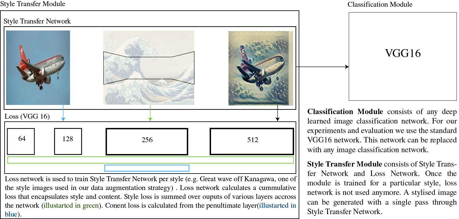
In this section, we propose a modular design for using style transfer as data-augmentation technique. Figure 2 summarises the modular architecture we followed for creating our data augmentation strategy. We choose the network designed in [Engstrom, 2016] for our style transfer module. The reasons for this choice, architecture and implementation of the network are explained in subsection 3.1. For testing the data augmentation technique we use the classification module. In our experiments we used the standard VGG16 from [Simonyan and Zisserman, 2014] explained in section 3.2. In section 3.3 we briefly explain the datasets used for evaluation of our strategy.

3.1 Style Transfer Architecture

For style transfer to be as viable as the other traditional data augmentation strategies (crop, flip etc.) we need a fast running solution. There has been successful style transfer solutions using CNNs but they are considerably slow [Gatys et al., 2016]. To alleviate this problem we choose a generative architecture that only needs a forward pass to compute a stylised image [Engstrom, 2016]. This network consists of a generative Style Transfer Network coupled with a Loss Network that computes a cumulative loss which can account for both style from the style image and content from the training image. In the following subsections (3.1.1, 3.1.2) we will look at architectures of the Style Transfer Network and Loss Network.

3.1.1 Transformation Network

For the transformation network, we follow the state-of-the-art implementation from the work [Engstrom, 2016] and [Sam and Michael, 2016], with changes to hyper parameters based on our experiments.

Five residual blocks are used in the style transformation network to avoid optimisation difficulty when the network gets deep [He et al., 2016]. Other none residual convolutional layers are followed by Ulyanov’s instance normalisation [Ulyanov et al., 2016b] and ReLU layers. At the output layer, a scaled tanh is used to get an output image with pixels in the range from 0 to 255.

This network is trained coupled with the Loss Network (described in the following subsection) using stochastic gradient descent [Bottou, 2010] to minimise a weighted combination of loss functions. We treat the overall loss as a linear combination of the content reconstruction loss and style reconstruction loss. The weights of two losses can be fine-tuned depending on the preference. By minimising the overall loss we can get a model well trained per style.

3.1.2 Loss Network

Since we already define the transformation network that can generate stylised images, we also need to create a loss network that is used to represent loss function to evaluate the generated images and use the loss to optimise the style transfer network based on stochastic gradient descent.

We use a deep convolutional neural network $\theta$ pretrained for image classification on imageNet to measure the texture and content differences between the generated image and the target image. Recent work has shown that deep convolutional neural networks can encode the texture information and high-level content information in the feature maps [Gatys et al., 2015][Mahendran and Vedaldi, 2015]. Based on this finding, we define a content reconstruction loss $\ell_{c}^{\theta}$ and a style reconstruction loss $\ell_{style}^{\theta}$ in the loss network and use their weighted sum to measure the total difference between the stylised image and the image we want to get. For every style, we train the transformation network with the same pretrained loss network.

Content Reconstruction Loss: To achieve that, an image needs to be reconstructed from the image information encoded in the neural network, i.e., computing an approximate inverse from the feature map. Given an image $\vec{x}$, the image will go through the CNN model and be encoded in each layer by the filter responses to it. We use $F^{l}$ to store the feature maps in a layer $l$ where $F_{ij}^{l}$ is the feature map of the $i^{th}$ filter at position $j$ in layer $l$. Let $P^{l}$ be the feature maps for the content image in layer $l$, and we can update the pixels of image $x$ to minimise the loss $\mathcal{L}$ to make sure these two images have the similar feature maps in the network and thus have the similar semantic content:

$$\mathcal{L}_{content}=\frac{1}{2}\sum_{i,j}(F_{ij}^{l}-P_{ij}^{l})^{2}$$ (1)

Style Reconstruction Loss: We also want the generated images to have similar texture as the style target image, so we want to penalise the style differences with the style reconstruction loss. The feature maps in a few layers of a trained network are used for representing the texture by the correlations between them. Instead of using these feature maps directly, the correlations between the different channels of the feature maps are given by Gram matrix $G^{l}$, where the $G_{i,j}^{l}$ is the inner product between the vectorised $i^{th}$ feature map and $j^{th}$ feature map in layer $l$:

$$G_{i,j}^{l}=\sum_{k}F_{ik}^{l}F_{jk}^{l}$$ (2)

The original texture is passed through the CNNs and the Gram matrices $G^{l}$ on the feature responses of some layers are computed. We can pass a white noise image through the CNNs and compute the Gram matrix difference on every layer included in the texture model as the loss. If we use this loss to perform gradient on the white noise image and try to minimise the Gram matrix difference, we can find a new image that has the same style as the original image texture. The loss is computed by the mean-squared distance between the Gram matrix of two images. So let $A^{l}$ and $G^{l}$ be the Gram matrix of two images in layer $l$, the loss of that layer equal:

$$E_{l}=\frac{1}{4N^{2}_{l}M^{2}_{l}}\sum_{i,j}(G^{l}_{ij}-A^{l}_{ij})^{2}$$ (3)

and the loss for all chosen layers:

$$\mathcal{L}_{style}=\sum_{l=0}^{L}w_{l}E_{l}$$ (4)

Total Variation Regularization: We also follow prior work [Gatys et al., 2016] and make use of total variation regularizer $\mathcal{L}_{TV}$ to gain more spatial smoothness in the output image $\hat{y}$.

Terms Balancing: As we have above definitions, generating an image $\hat{y}$ can be seen as solving the optimising problem in the style transfer module in figure 2. We initialise the image with white noise, and the work [Gatys et al., 2016] found that the initialisation has a minimal impact on the final results. $\lambda_{c}$, $\lambda_{s}$, and $\lambda_{TV}$ are hyperparameters that we can tune according to the monitoring of the results. To get the stylised image, we need to minimise a weighted combination of two loss functions and the regularization term:

$$\hat{y}=\operatorname*{argmin}_{y}\lambda_{c}\mathcal{L}_{content}+\lambda_{s}\mathcal{L}_{style}+\lambda_{TV}\mathcal{L}_{TV}$$ (5)

3.2 Image Classification

To evaluate the effectiveness of this design, we perform image classification tasks with the stylised images. In a image classification task, for each given image, the programs or algorithms need to produce the most reasonable object categories [Russakovsky et al., 2015]. The performance of the algorithm will be evaluated based on if the predicated category matches the ground truth label for the image. Since we will provide input images from multiple categories, the overall performance of an algorithm is the average score of overall test images.

Once we train the transformation network that can generate the stylised images, we apply it to the training dataset to create a larger dataset. The stylized images are saved on the disk with the ground truth categories. We then use them with their original images to train the neural networks to solve the image classification problems. In this research, the model we chose is VGGNet, which is a simple but effective model [Simonyan and Zisserman, 2014]. Their team got the first place in the localisation and the second place in the classification task in ImageNet Challenge 2014. This model strictly used $3\times 3$ filters with stride and pad of 1, along with $2\times 2$ max-pooling layers with stride 2. 3 $3\times 3$ convolutional layers back to back have an effective receptive field of $7\times 7$. Compared with one $7\times 7$ filter, $3\times 3$ filter size can have the same effective receptive field with fewer parameters.

To fully understand the effectiveness of the style transfer and explore how useful style transfer can be compared and combined with other traditional data augmentation approaches for image classification problem, we need to experiment from multiple perspectives. The first experiments are to use traditional transformations alone. For each input image, we generate a set of duplicate images that are shifted, rotated, or flipped from the original image. Both the original image and duplicates are fed into the neural net to train the model. The classification performance will be measured on the validation dataset as the baseline to compare these augmentation strategies. The pipeline can be found in Figure 2. The second experiments are to apply the well-trained transformation network to augment the training dataset. For each input image, we select a style image from a subset of different styles from famous artists and use the transformation network to generate new images from the original image. We store the newly generated images on the disk, and both original and stylised images are fed to the image classification network. To explore if we can get better results, we go further to combine two approaches to get more images in training dataset .

3.3 Dataset and Image Styles

The transformation network is trained on the COCO 2014 collection [Lin et al., 2014] containing more than 83k training images, which are enough to get the transformation network well trained. Since these images are used to feed the transformation network, we ignored the label information during training.

Two different datasets are used for images clasification tasks, caltech 101 [Fei-Fei et al., 2006] and caltech 256 [Griffin et al., 2007]. We keep training and testing on a fixed number of images and repeating the experiment with different augmented data and compare the results with others. The images are divided by a 70:30 split between training and validation for both datasets.

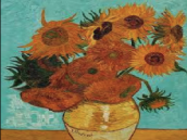
For the chosen styles, we try to select the images that look very different. At last, eight different images were chosen as the style input to train the transformation network. All styles can be found in the GitHub repo. https://github.com/zhengxu001/neural-data-augmentation.

4 EXPERIMENTS

This section presents the evaluation of style transfer for data augmentation. We evaluate the results from multiple perspectives based on the classification Top-1 accuracy of VGGNet. The results of experiments on traditional augmentation are collected as the baseline. We then do experiments on every single style and some combined styles. We also combine the traditional methods with our style transfer method to verify their effectiveness and see if we can improve on previous methods.

4.1 Traditional Image Augmentation

We first used the pretrained VGGNet without any data augmentation and reached a classification accuracy of 83.34% in one hour of training time. We then apply two different traditional image augmentation strategies, Flipping and Rotation, to train the model. Finally, we combine both strategies. Detailed results can be found in table 1. We found the model itself works the best without any augmentation. Using Flipping as data augmentation strategy gives very similar results, however the combination of Rotation and Flipping significantly reduces classification accuracy to 77%. Adding Rotation as data augmentation does not seem to help for classification, as is also shown in our following experiments.

Traditional Image Augmentation
Style Name	Result
None	0.8334
Flipping	0.8305
FlippingRotation	0.77

Table 1: Traditional Image Augmentation

4.2 Single Style

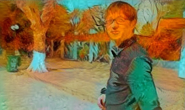
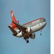
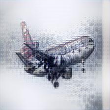
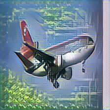
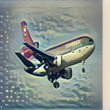
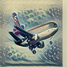
We select eight different styles that look different from each other to train the transformation network. All styles can be found in the Appendix. We feed each of the images in the training set to the eight fully trained transformation networks to generate eight stylised images. Both the original images and the stylised images are fed to VGGNet to train the network and the best validation accuracy from all epochs is recorded. The results for each style can be found in table 2. Compared with the traditional strategies, we can see that 7 out of 8 styles work better than the traditional strategies. It can also be seen that the Snow style works the best, reaching an accuracy of 85.26%, whereas YourName style only reaches 82.61%. This is due to the addition of too much noise and colour to the original images for that particular style. In figure 3 a comparison between the original image and two different stylised images is shown. As can be seen, YourName style adds too many colours and shapes on the original image, which explains the bad performance in terms of the image classification accuracy.

Single Style with VGG16 and Caltech 101
Style Name	Result
Snow	0.8526
RainPrincess	0.8494
Scream	0.8490
Wave	0.8468
Sunflower	0.8461
LAMuse	0.8436
Udnie	0.8404
Your Name	0.8261

Table 2: Single Style Transfer Augmentation

(a) Original

(b) Snow

(c) YourName

Figure 3: Comparison between the original image and two stylized images. YourName style adds too many colours and shapes on the original image, which explains the bad performance in terms of the image classification accuracy.

4.3 Combined Methods

To evaluate the combination of two different styles, we take the original images and feed them to two different transformation networks and generate two stylized images for each input image. We then merge the stylized images and original images to compose the final training dataset. This gives us three times the number of images than the original dataset. We use this augmented data set to train the VGGNet model. We also try to combine the traditional augmentation methods with style transfer together and evaluate the performance. The results can be found in table 3.

Combined Method
Traditional Method	Style	Result
Flipping	None	0.8305
Flipping	Scream	0.8454
Flipping	Wave	0.8486
Flipping	ScreamWave	0.845
FlippingRotation	None	0.7521
FlippingRotation	Wave	0.7837
FlippingRotation	Scream	0.7862
FlippingRotation	ScreamWave	0.7942

Table 3: Combined Style Transfer Augmentation

We notice a very slight increase in performance of the combined style (ScreamWave) over the single styles. We further notice that adding Flipping as a data augmentation strategy degrades the performance, although to a lesser degree for the combined style.

4.4 Content Weights Change

In this experiment, we change the proportion of content weights and style weight in the transformation network to evaluate the impact on the performance. We increased the content weight to create a new style named Wave2. As can be seen from the table 4, no significant change can be observed for a change in content weights. As can be seen in figure 4, the images for the two content weights look very similar to each other, which explains the minimal impact in our experiments. In future work we would like to examine this effect further with more content weights.

Different Content Weights
Traditional Method	Style Name	Result
None	Wave	0.8468
None	Wave2	0.8417

Table 4: Wave2 gets more content weight than Wave

(a) Original

(b) Wave2

(c) Wave

Figure 4: Comparison between the original image (airplane) and stylized images with different content weights. (a) is the original image. Wave2 (b) has more content weight than Wave (c). Two stylized images look similar to each other.

4.5 VGG19

To evaluate the generalisation of our approach over network architectures, we used VGG19 as a classification network and duplicated our experiments. The results can be found in table 5.

Experiments on VGG19
Traditional Method	Style Name	Result
None	None	0.8450
Flipping	None	0.8367
None	Wave	0.8425
Flipping	Wave	0.8581
None	Scream	0.8446
Flipping	Scream	0.8465
None	None	0.62
Flipping	None	0.6666
None	Scream	0.6313
Flipping	Scream	0.6728
None	Wave	0.6272
Flipping	Wave	0.6632

Table 5: Experiments on VGG19 with Caltech datasets

The baseline classification accuracy for Caltech 101 is 84.5%. Based on this number, there are some interesting findings in line with the VGG16. Using Wave or Flipping itself does not improve the performance of VGG19, but if we combine Flipping with Wave we can get a considerable improvement, with accuracy reaching 85.81%.

Similar results can be seen for our experiments on Caltech 256. The use of Flipping as data augmentation gives an accuracy of 66.66%, while the use of Scream gives at 63.13%. However, if we combine the two approaches, we can get an accuracy of 67.28%. The combination between Flipping and Wave gives 66.32% accuracy which is higher than for Wave alone.

The experiments performed on VGG19 show that the style transfer is still an effective data augmentation method, which can be combined with the traditional approaches to further improve the performance.

5 CONCLUSIONS

In this paper, we proposed a novel data augmentation approach based on neural style transfer algorithm. From our experiments, we observe that this approach is an effective way to increase the performance of CNNs in image classification tasks. The accuracy for VGG16 is increased to 85.26% from 83.34% while for VGG19 the accuracy increased to 85.81% from 84.50%. We also found that we can combine this new approach with traditional methods like flipping, rotation etc. to boost the performance.

We tested our method only for image classification task. As a future work, it would be interesting to try it out for other computer vision tasks such as segmentation, detection etc. The set of styles is also limited. Even though we tried to select images of different styles, we did not classify the images according to their category. A more elaborate set of styles might train more robust models. Another limitation of this approach is the speed of training, which is quite slow. However, once trained, the inference can still be fast as it does not involve augmentation.

Our approach is independent of the architecture. Better and faster models for style transfer will enable more diverse and robust augmentation for a CNN. We hope that the proposed approach will be useful for computer vision research in future.

REFERENCES

- Bottou, 2010 Bottou, L. (2010). Large-scale machine learning with stochastic gradient descent. In Proceedings of COMPSTAT’2010, pages 177–186. Springer.
- Caruana et al., 2001 Caruana, R., Lawrence, S., and Giles, C. L. (2001). Overfitting in neural nets: Backpropagation, conjugate gradient, and early stopping. In Advances in neural information processing systems, pages 402–408.
- Chalasani et al., 2018 Chalasani, T., Ondrej, J., and Smolic, A. (2018). Egocentric gesture recognition for head mounted ar devices. In Adjunct Proceedings of the IEEE International Symposium for Mixed and Augmented Reality 2018 (To appear).
- Chen and Hsu, 2016 Chen, Y.-L. and Hsu, C.-T. (2016). Towards deep style transfer: A content-aware perspective. In BMVC.
- Deng et al., 2009 Deng, J., Dong, W., Socher, R., Li, L.-J., Li, K., and Fei-Fei, L. (2009). Imagenet: A large-scale hierarchical image database. In Computer Vision and Pattern Recognition, 2009. CVPR 2009. IEEE Conference on, pages 248–255. Ieee.
- Dumoulin et al., 2016 Dumoulin, V., Shlens, J., and Kudlur, M. (2016). A learned representation for artistic style. arXiv e-prints, abs/1610.07629.
- Engstrom, 2016 Engstrom, L. (2016). Fast style transfer. https://github.com/lengstrom/fast-style-transfer/.
- Fei-Fei et al., 2006 Fei-Fei, L., Fergus, R., and Perona, P. (2006). One-shot learning of object categories. IEEE transactions on pattern analysis and machine intelligence, 28(4):594–611.
- Gatys et al., 2015 Gatys, L., Ecker, A. S., and Bethge, M. (2015). Texture synthesis using convolutional neural networks. In Advances in Neural Information Processing Systems, pages 262–270.
- Gatys et al., 2016 Gatys, L. A., Ecker, A. S., and Bethge, M. (2016). Image style transfer using convolutional neural networks. In Computer Vision and Pattern Recognition (CVPR), 2016 IEEE Conference on, pages 2414–2423. IEEE.
- Griffin et al., 2007 Griffin, G., Holub, A., and Perona, P. (2007). Caltech-256 object category dataset.
- He et al., 2016 He, K., Zhang, X., Ren, S., and Sun, J. (2016). Deep residual learning for image recognition. In Proceedings of the IEEE conference on computer vision and pattern recognition, pages 770–778.
- Jing et al., 2017 Jing, Y., Yang, Y., Feng, Z., Ye, J., and Song, M. (2017). Neural style transfer: A review. CoRR, abs/1705.04058.
- Johnson et al., 2016 Johnson, J., Alahi, A., and Fei-Fei, L. (2016). Perceptual losses for real-time style transfer and super-resolution. In European Conference on Computer Vision, pages 694–711. Springer.
- Krizhevsky et al., 2012 Krizhevsky, A., Sutskever, I., and Hinton, G. E. (2012). Imagenet classification with deep convolutional neural networks. In Advances in neural information processing systems, pages 1097–1105.
- Kyprianidis et al., 2013 Kyprianidis, J. E., Collomosse, J., Wang, T., and Isenberg, T. (2013). State of the” art”: A taxonomy of artistic stylization techniques for images and video. IEEE transactions on visualization and computer graphics, 19(5):866–885.
- Li and Wand, 2016 Li, C. and Wand, M. (2016). Precomputed real-time texture synthesis with markovian generative adversarial networks. In European Conference on Computer Vision, pages 702–716. Springer.
- Li et al., 2017 Li, Y., Wang, N., Liu, J., and Hou, X. (2017). Demystifying neural style transfer. arXiv preprint arXiv:1701.01036.
- Lin et al., 2014 Lin, T., Maire, M., Belongie, S. J., Bourdev, L. D., Girshick, R. B., Hays, J., Perona, P., Ramanan, D., Dollár, P., and Zitnick, C. L. (2014). Microsoft COCO: common objects in context. CoRR, abs/1405.0312.
- Mahendran and Vedaldi, 2015 Mahendran, A. and Vedaldi, A. (2015). Understanding deep image representations by inverting them. In Proceedings of the IEEE conference on computer vision and pattern recognition, pages 5188–5196.
- Perez and Wang, 2017 Perez, L. and Wang, J. (2017). The effectiveness of data augmentation in image classification using deep learning. arXiv preprint arXiv:1712.04621.
- Risser et al., 2017 Risser, E., Wilmot, P., and Barnes, C. (2017). Stable and controllable neural texture synthesis and style transfer using histogram losses. arXiv preprint arXiv:1701.08893.
- Russakovsky et al., 2015 Russakovsky, O., Deng, J., Su, H., Krause, J., Satheesh, S., Ma, S., Huang, Z., Karpathy, A., Khosla, A., Bernstein, M., Berg, A. C., and Fei-Fei, L. (2015). ImageNet Large Scale Visual Recognition Challenge. International Journal of Computer Vision (IJCV), 115(3):211–252.
- Sam and Michael, 2016 Sam, G. and Michael, W. (2016). Training and investigating residual nets. http://torch.ch/blog/2016/02/04/resnets.html.
- Simonyan and Zisserman, 2014 Simonyan, K. and Zisserman, A. (2014). Very deep convolutional networks for large-scale image recognition. arXiv preprint arXiv:1409.1556.
- Ulyanov et al., 2016a Ulyanov, D., Lebedev, V., Vedaldi, A., and Lempitsky, V. S. (2016a). Texture networks: Feed-forward synthesis of textures and stylized images. In ICML, pages 1349–1357.
- Ulyanov et al., 2016b Ulyanov, D., Vedaldi, A., and Lempitsky, V. S. (2016b). Instance normalization: The missing ingredient for fast stylization. CoRR, abs/1607.08022.
- Vasconcelos and Vasconcelos, 2017 Vasconcelos, C. N. and Vasconcelos, B. N. (2017). Increasing deep learning melanoma classification by classical and expert knowledge based image transforms. CoRR, abs/1702.07025, 1.
- Yin, 2016 Yin, R. (2016). Content aware neural style transfer. arXiv preprint arXiv:1601.04568.
- Zeiler and Fergus, 2014 Zeiler, M. D. and Fergus, R. (2014). Visualizing and understanding convolutional networks. In European conference on computer vision, pages 818–833. Springer.
- Zhu et al., 2017 Zhu, J.-Y., Park, T., Isola, P., and Efros, A. A. (2017). Unpaired image-to-image translation using cycle-consistent adversarial networks. arXiv preprint.