Response of a uniformly accelerated Unruh-DeWitt detector in polymer quantization

Abstract

If an Unruh-DeWitt detector moves with a uniform acceleration in Fock-space vacuum, then the transition rate of the detector is proportional to the thermal spectrum. It is well known that the transition rate of the detector crucially depends on the two-point function along the detectors trajectory and in order to compute it the standard “$i\epsilon$” regularization is used for Fock space. Numerically, we show here that the regulator $\epsilon$ is generic in polymer quantization, the quantization method used in loop quantum gravity with a finite value $\epsilon\approx 2.16$, which leads to non-thermal spectrum for the uniformly accelerated detector. We also discuss the response of a spatially smeared detector.

I Introduction

Minkowski vacuum is perceived by an observer accelerating with a uniform acceleration $a$ as a thermal distribution with temperature $T=a/2\pi k_{B}$, the Unruh temperature, where $k_{B}$ is the Boltzmann constant Fulling (1973); Unruh (1976); Crispino et al. (2008); De Bièvre and Merkli (2006); Takagi (1986); Longhi and Soldati (2011); Davies (1975); Birrell and Davies (1984); Banerjee et al. (2016); Omkar et al. (2016); Banerjee et al. (2017). The Unruh effect can be approached from different perspectives. A common approach is the application of Bogoliubov transformations. The expectation value of the number density operator in the Fock vacuum state, as perceived by an accelerated observer, has the form of a blackbody distribution at Unruh temperature. The Unruh effect appears to explicitly depend on the contributions from trans-Planckian modes, as observed by an inertial observer. This thus provides a potential candidate for exploring the implications of possible Planck-scale physics Nicolini and Rinaldi (2011); Padmanabhan (2010); Agullo et al. (2008); Chiou (2018); Alkofer et al. (2016), such as those falling within the ambit of quantum gravity.

Another approach, adopted here, is to compute the response function of the Unruh-DeWitt detector moving along the trajectory of an accelerated observer DeWitt (1980); Hinton (1983); Schlicht (2004); Louko and Satz (2006); Unruh and Wald (1984); Louko (2014); Sriramkumar and Padmanabhan (1996); Agullo et al. (2010); Fewster et al. (2015); Satz (2007); Langlois (2006); Hümmer et al. (2016). In this approach, one considers a two-level quantum mechanical detector which weakly couples to the ambient environment, such as a scalar matter field. By computing the transition probability of the detector between the energy levels and comparing with the spontaneous and induced emission or absorption, one can understand the state of the scalar matter field. In particular, the detector response function depends upon the Wightman (two-point) function of the scalar field.

Polymer (loop) quantization Ashtekar et al. (2003); Halvorson (2004) is used as a quantization technique in loop quantum gravity Ashtekar and Lewandowski (2004); Rovelli (2004); Thiemann (2007). It has an inbuilt (dimension-full) parameter apart from the Planck constant $\hbar$. This new scale corresponds to Planck length $L_{p}$ in the context of full quantum gravity. Further, here both position and momentum operators cannot be simultaneously defined. These features make polymer quantization unitarily inequivalent to Schrödinger quantization Ashtekar et al. (2003). Here we compute the response function of an Unruh-DeWitt detector in the context of polymer quantization of scalar field weakly coupled to the detector.

The plan of the paper is as follows. In section II, we briefly discuss about spacetime as seen by a uniformly accelerating observer in Minkowski spacetime $i.e.,$ the Rindler observer and its trajectory. Next, in section III, we consider polymer quantization of a massless free scalar field in the canonical approach. The properties of the Unruh-DeWitt detector are then studied. Subsequently, we study the behaviour of the Fock space two-point function analytically by considering the standard “$i\epsilon$” regularization. By comparing the numerically computed polymer and Fock space two-point functions we show that the regulator $\epsilon$, used for the standard regularization for Fock space, is generic in the case of polymer-two-point function with a finite value $\epsilon\approx 2.16$. Thus, a generic cut-off is seen to emerge in polymer quantization. Then we compute the induced transition rate of the Unruh-DeWitt detector along the Rindler trajectory. We show that, in Fock quantization, the induced transition rate is proportional to Planck distribution. However, in polymer quantization, due to the large value of the generic regulator $\epsilon$, the induced transition rate deviates from the Planck distribution. Next, we compute the induced transition rate by considering spatially smeared detector in both Fock and polymer quantizations. Finally, we make our conclusions.

II Rindler Spacetime

The spacetime of an observer who is moving with a uniform acceleration in Minkowski spacetime can be described by the so-called Rindler metric. Using conformal Rindler coordinates $\bar{x}^{\alpha}=(\tau,\xi,y,z)\equiv(\tau,\vec{\xi})$ together with natural units ($c=\hbar=1$) the Rindler metric can be expressed as Rindler (1966)

$$ds^{2}=e^{2a\xi}\left(-d\tau^{2}+d\xi^{2}\right)+dy^{2}+dz^{2}\equiv g_{\alpha\beta}d\bar{x}^{\alpha}d\bar{x}^{\beta}~{},$$ (1)

where the parameter $a$ is the magnitude of acceleration 4-vector. With respect to an inertial observer the Minkowski metric with Cartesian coordinates $x^{\mu}=(t,x,y,z)\equiv(t,\mathbf{x})$ would appear as $ds^{2}=\eta_{\mu\nu}dx^{\mu}dx^{\nu}=-dt^{2}+dx^{2}+dy^{2}+dz^{2}$. If the uniformly accelerated observer i.e., Rindler observer moves along positive x-axis with respect to the inertial observer, the coordinates are related each other by

$$t=\frac{1}{a}e^{a\xi}\sinh a\tau~{},~{}~{}~{}x=\frac{1}{a}e^{a\xi}\cosh a\tau~{},$$ (2)

Here, $y$ and $z$ coordinates are the unaffected. It can be seen from the equation (2) that only a wedge-shaped section of Minkowski spacetime is covered by Rindler spacetime, called the Rindler wedge.

III Scalar field

We consider a massless scalar field $\Phi(x)$ weakly coupled to the detector in Minkowski spacetime. The action for corresponding scalar field dynamics is

$$S_{\Phi}=\int d^{4}x\left[-\frac{1}{2}\sqrt{-\eta}\eta^{\mu\nu}\partial_{\mu}\Phi(x)\partial_{\nu}\Phi(x)\right]~{}.$$ (3)

The field Hamiltonian is

$$H_{\Phi}=\int d^{3}\mathbf{x}\left[\frac{\Pi^{2}}{2\sqrt{q}}+\frac{\sqrt{q}}{2}q^{ab}\partial_{a}\Phi\partial_{b}\Phi\right]~{},$$ (4)

where $q_{ab}$ is the metric on spatial hyper-surfaces labeled by $t$. Poisson bracket between the field $\Phi=\Phi(t,\mathbf{x})$ and its conjugate field momentum $\Pi=\Pi(t,\mathbf{x})$ is

$$\{\Phi(t,\mathbf{x}),\Pi(t,\mathbf{y})\}=\delta^{3}(\mathbf{x}-\mathbf{y})~{},$$ (5)

where $\delta^{3}(\mathbf{x}-\mathbf{y})$ is the Dirac delta.

III.1 Fourier modes

Here we express Fourier modes for the scalar field and its conjugate field momentum as

$$\Phi=\frac{1}{\sqrt{V}}\sum_{\mathrm{k}}\tilde{\phi}_{\mathrm{k}}(t)e^{i\mathrm{k}\cdot\mathbf{x}},~{}\Pi=\frac{1}{\sqrt{V}}\sum_{\mathrm{k}}\sqrt{q}~{}\tilde{\pi}_{\mathrm{k}}(t)e^{i\mathrm{k}\cdot\mathbf{x}},$$ (6)

where $V=\int d^{3}\mathbf{x}\sqrt{q}$ is the spatial volume. In Minkowski spacetime, as the space is non-compact, the spatial volume would normally diverge. In order to avoid this issue, it is convenient to use a fiducial box of finite volume. Kronecker and Dirac delta functions then can be expressed as $\int d^{3}\mathbf{x}\sqrt{q}~{}e^{i(\mathrm{k}-\mathrm{k}^{\prime})\cdot\mathbf{x}}=V\delta_{\mathrm{k},\mathrm{k}^{\prime}}$ and $\sum_{\mathrm{k}}e^{i\mathrm{k}\cdot(\mathbf{x}-\mathbf{y})}=V\delta^{3}(\mathbf{x}-\mathbf{y})/\sqrt{q}$, respectively. The field Hamiltonian (4) can be expressed as $H_{\Phi}=\sum_{\mathrm{k}}\mathcal{H}_{\mathrm{k}}$, where Hamiltonian density for the $\mathrm{k}-$th Fourier mode is

$$\mathcal{H}_{\mathrm{k}}=\frac{1}{2}\tilde{\pi}_{-\mathrm{k}}\tilde{\pi}_{\mathrm{k}}+\frac{1}{2}|\mathrm{k}|^{2}\tilde{\phi}_{-\mathrm{k}}\tilde{\phi}_{\mathrm{k}}~{}.$$ (7)

Poisson brackets between these Fourier modes and their conjugate momenta are given by

$$\{\tilde{\phi}_{\mathrm{k}},\tilde{\pi}_{-\mathrm{k}^{\prime}}\}=\delta_{\mathrm{k},\mathrm{k}^{\prime}}~{}.$$ (8)

One usually redefines the complex-valued modes $\tilde{\phi}_{\mathrm{k}}$ and momenta $\tilde{\pi}_{\mathrm{k}}$ in terms of the real-valued functions $\phi_{\mathrm{k}}$ and $\pi_{\mathrm{k}}$ in order to satisfy the reality condition of the scalar field $\Phi$. Therefore, the corresponding Hamiltonian density and Poisson brackets become

$$\mathcal{H}_{\mathrm{k}}=\frac{1}{2}\pi_{\mathrm{k}}^{2}+\frac{1}{2}|\mathrm{k}|^{2}\phi_{\mathrm{k}}^{2}~{}~{}~{};~{}~{}~{}\{\phi_{\mathrm{k}},\pi_{\mathrm{k}^{\prime}}\}=\delta_{\mathrm{k},\mathrm{k}^{\prime}}~{},$$ (9)

which is the standard Hamiltonian for a system of decoupled harmonic oscillators. The relevant eigenvalue equation is $\hat{\mathcal{H}}_{\mathrm{k}}|n_{\mathrm{k}}\rangle=E_{n}^{(\mathrm{k})}|n_{\mathrm{k}}\rangle$, where $|0_{\mathrm{k}}\rangle$ is the vacuum state of the $k^{th}$ mode. The vacuum state of the scalar field is $|0\rangle=\Pi_{\mathrm{k}}\otimes|0_{\mathrm{k}}\rangle$.

IV Unruh-DeWitt Detector

Unruh-Dewitt detector is a point-like quantum mechanical system which has two internal energy levels. Here we study the response function of the Unruh-DeWitt detector which interacts weakly with the scalar field via a linear coupling. The energy eigenvalue equation of the detector is

$$\hat{H}_{0}|g\rangle=\omega_{g}|g\rangle~{}~{};~{}~{}\hat{H}_{0}|e\rangle=\omega_{e}|e\rangle~{},$$ (10)

where $\hat{H}_{0}$ is the unperturbed Hamiltonian of the detector and $|g\rangle$ and $|e\rangle$ represent the ground and excited states, respectively. The energy gap is

$$\omega\equiv\left(\omega_{e}-\omega_{g}\right)>0~{}.$$ (11)

The interaction Hamiltonian of the Unruh-DeWitt detector is taken as

$$\hat{H}_{int}(\tau)=\lambda~{}\hat{\mu}(\tau)\hat{\Phi}(x(\tau))~{},$$ (12)

where $\lambda$ denotes the coupling constant and $\hat{\mu}(\tau)$ is the monopole moment operator of the detector. The detector’s trajectory $x^{\mu}(\tau)$ is parametrized using the proper time $\tau$. Hence, the total detector Hamiltonian is

$$\hat{H}=\hat{H}_{0}+\hat{H}_{int}~{}.$$ (13)

It is convenient to work in the interaction picture, in which the time evolution operator of the detector is given by

$$U(\tau_{f},\tau_{i})=1-i\int_{\tau_{i}}^{\tau_{f}}d\tau^{\prime}U(\tau^{\prime},\tau_{i})\hat{H}_{I}(\tau^{\prime})~{}.$$ (14)

If the state of the scalar field is $|\Xi_{\tau}\rangle$, the combined state of the detector and the scalar field at a given proper time $\tau$ is

$$|\psi,\Xi;\tau\rangle\equiv|\psi_{\tau}\rangle_{I}\otimes|\Xi_{\tau}\rangle~{}.$$ (15)

The transition amplitude from the state $|g,\Xi_{i};0\rangle$ to $|e,\Xi_{f};\tau\rangle$ can be expressed as

$$\mathop{Amp}=-i\lambda\int_{0}^{\tau}d\tau^{\prime}\langle e,\Xi_{f};\tau|\hat{\mu}_{I}(\tau^{\prime})\hat{\Phi}(x(\tau^{\prime}))|g,\Xi_{i};0\rangle~{},$$ (16)

where $\hat{\mu}_{I}(\tau)$ is the monopole moment operator in the interaction picture and the corresponding probability of transition is

$$\mathcal{P}_{|g,\Xi_{i};0\rangle\to|e,\Xi_{f};\tau\rangle}=|Amp|^{2}~{}.$$ (17)

Now if the detector initially is at ground state and the scalar field is in its vacuum state i.e., $|\Xi_{i}\rangle=|0\rangle$, then the transition probability at a time $\tau$ for the detector being in the excited state $|e\rangle$ for all possible field states is

$$\mathcal{P}_{\omega}(\tau,0)\equiv\mathcal{P}_{|g;0\rangle\to|e;\tau\rangle}=\sum_{\{|\Xi_{f}\rangle\}}\mathcal{P}_{|g,\Xi_{i};0\rangle\to|e,\Xi_{f};\tau\rangle}~{}.$$ (18)

The transition probability (18) can be easily expressed in the form of

$$\mathcal{P}_{\omega}(\tau,0)=A_{0}\mathcal{F}_{\omega}(\tau,0)~{},$$ (19)

where $A_{0}=\lambda^{2}|\langle e|\hat{\mu}(0)|g\rangle|^{2}$. $A_{0}$ depends on the internal properties of the detector system. $\mathcal{F}_{\omega}(\tau,0)$ is the response function of the detector, and is

$$\mathcal{F}_{\omega}(\tau,0)=\int_{0}^{\tau}\int_{0}^{\tau}d\tau^{\prime}d\tau^{\prime\prime}e^{-i\omega(\tau^{\prime\prime}-\tau^{\prime})}~{}G(\tau^{\prime\prime},\tau^{\prime})~{},$$ (20)

where $G(\tau^{\prime\prime},\tau^{\prime})$ is the two-point function of the scalar field which can be expressed as

$$G(\tau^{\prime\prime},\tau^{\prime})=G(\tau^{\prime\prime}-\tau^{\prime})=\langle 0|\hat{\Phi}(x(\tau^{\prime\prime}))\hat{\Phi}(x(\tau^{\prime}))|0\rangle~{}.$$ (21)

We can now define the instantaneous transition rate by using equation (19) with a scaling, as

$$R_{\omega}(\tau,0)\equiv\left(\frac{2\pi}{A_{0}}\right)\frac{d\mathcal{P}_{\omega}}{d\tau}=2\pi\int_{-\tau}^{\tau}d\tau^{\prime}e^{-i\omega\tau^{\prime}}G(\tau^{\prime})~{},$$ (22)

which can be re-expressed as

$$R_{\omega}(\tau,0)=R_{\omega}^{0}+\Delta R_{\omega}(\tau)~{}.$$ (23)

The $R_{\omega}^{0}$ denotes the time independent part of the induced transition rate i.e., the non-transient part, which can be expressed as

$$R_{\omega}^{0}=2\pi\int_{-\infty}^{\infty}d\tau^{\prime}e^{-i\omega\tau^{\prime}}G(\tau^{\prime})~{}.$$ (24)

On the other hand, $\Delta R_{\omega}(\tau)$ denotes time-dependent i.e., transient part of the induced transition rate and it can be expressed as

$$\Delta R_{\omega}(\tau)=-2\pi\int_{\tau}^{\infty}d\tau^{\prime}\left[e^{-i\omega\tau^{\prime}}G(\tau^{\prime})+e^{i\omega\tau^{\prime}}G(-\tau^{\prime})\right]~{}.$$ (25)

$\Delta R_{\omega}(\tau)\to 0$ with increasing observation time i.e., $\tau\to\infty$.

IV.1 Two-point function

We can see from the equation (22) that induced transition rate of the Unruh-DeWitt detector is completely determined from the properties of the two-point function. The general form of two-point function can be written in terms of the Fourier modes (6) as

$$G(x,x^{\prime})=\langle 0|\hat{\Phi}(x)\hat{\Phi}(x^{\prime})|0\rangle=\frac{1}{V}\sum_{\mathrm{k}}D_{\mathrm{k}}(t,t^{\prime})e^{i{\mathrm{k}}\cdot(\mathbf{x}-\mathbf{x}^{\prime})},$$ (26)

where the matrix element $D_{\mathrm{k}}(t,t^{\prime})$ is given by

$$D_{\mathrm{k}}(t,t^{\prime})=\langle 0_{\mathrm{k}}|e^{i\hat{\mathcal{H}}_{\mathrm{k}}t}\hat{\phi}_{\mathrm{k}}e^{-i\hat{\mathcal{H}}_{\mathrm{k}}t}e^{i\hat{\mathcal{H}}_{\mathrm{k}}t^{\prime}}\hat{\phi}_{\mathrm{k}}e^{-i\hat{\mathcal{H}}_{\mathrm{k}}t^{\prime}}|0_{\mathrm{k}}\rangle.$$ (27)

Exploiting the independence of the Hamiltonians and the corresponding Poisson brackets (9) from the fiducial volume, the discrete summation over the modes can be replaced by an integration. Thus, the two-point function (26) can be expressed as

$$G(x,x^{\prime})=\int\frac{d^{3}\mathrm{k}}{(2\pi)^{3}}~{}D_{\mathrm{k}}(t,t^{\prime})~{}e^{i{\mathrm{k}}\cdot(\mathbf{x}-\mathbf{x}^{\prime})}~{}.$$ (28)

By expanding the state $\hat{\phi}_{\mathrm{k}}|0_{\mathrm{k}}\rangle$ in the basis of energy eigenstates as $\hat{\phi}_{\mathrm{k}}|0_{\mathrm{k}}\rangle=\sum_{n}b_{n}|n_{\mathrm{k}}\rangle$ and using energy spectrum of the Fourier modes, the matrix element $D_{\mathrm{k}}(t,t^{\prime})$ can be expressed as

$$D_{\mathrm{k}}(t-t^{\prime})\equiv D_{\mathrm{k}}(t,t^{\prime})=\sum_{n}|b_{n}|^{2}e^{-i\Delta E_{n}(t-t^{\prime})},$$ (29)

where $\Delta E_{n}\equiv E_{n}^{(\mathrm{k})}-E_{0}^{(\mathrm{k})}$ and $b_{n}=\langle n_{\mathrm{k}}|\hat{\phi}_{\mathrm{k}}|0_{\mathrm{k}}\rangle$. We can see that the matrix element $D_{\mathrm{k}}(t-t^{\prime})$ depends only on magnitude $|\mathrm{k}|$. Therefore, one can carry out the angular integration using polar coordinates, and the reduced two-point function (28) can be expressed as

$$G(x,x^{\prime})=G_{+}-G_{-}~{},$$ (30)

where

$$G_{\pm}=\frac{i}{4\pi^{2}|\Delta\mathbf{x}|}\int dk~{}kD_{k}(\Delta t)~{}e^{\mp ik|\Delta\mathbf{x}|}~{},$$ (31)

with $k=|\mathrm{k}|$, $\Delta\mathbf{x}=\mathbf{x}-\mathbf{x}^{\prime}$ and $\Delta t=t-t^{\prime}$.

V Fock quantization: Detector Response

In Fock quantization, the energy spectrum and the coefficients $b_{n}$ (29) of the Fourier modes (9) of the scalar field are given by

$$E^{n}_{\mathrm{k}}=\left(n+\frac{1}{2}\right)|\mathrm{k}|~{}~{};~{}~{}\Delta E_{n}=n|\mathrm{k}|~{}~{};~{}~{}b_{n}=\frac{\delta_{1,n}}{\sqrt{2|\mathrm{k}|}}~{}.$$ (32)

Using above equation (32), the two-point function (30) then reduces to its standard form

$$G(x,x^{\prime})=\frac{1}{4\pi^{2}\left[-(\Delta t-i\epsilon)^{2}+|\Delta\mathbf{x}|^{2}\right]}~{},$$ (33)

where $\Delta x^{2}=-\Delta t^{2}+|\Delta\mathbf{x}|^{2}$ is the Lorentz invariant spacetime interval. Further, $\epsilon$ is a small, positive parameter that is introduced as the standard integral regulator, $i.e$, as an additional term $e^{-\epsilon k}$ in the integrand of Eq. (31).

Now we compute the transition rate of an Unruh-DeWitt detector which moves along a Rindler trajectory given by $x_{d}^{\mu}(\tau)=(\sinh(a\tau)/a,\cosh(a\tau)/a,0,0)$. Defining a new variable $\rho=e^{a\tau}$, the time interval $\Delta t$ and spatial separation $|\Delta\mathbf{x}|$ can be expressed as

$$\Delta t=\frac{(\rho^{2}-1)}{2a\rho}~{}~{},~{}~{}|\Delta\mathbf{x}|=\frac{(\rho-1)^{2}}{2a\rho}~{},$$ (34)

and the corresponding two-point function (33) becomes

$$G(\rho)=-\frac{a^{2}~{}\rho}{4\pi^{2}\left(\rho-1-i\epsilon\right)^{2}}~{}.$$ (35)

Then the non-transient part of the transition rate (24) can be expressed as

$$R_{\omega}^{0}=-\frac{a}{2\pi}\int_{0}^{\infty}d\rho\frac{\rho^{-i\omega/a}}{\left(\rho-1-i\epsilon\right)^{2}}\equiv\int_{0}^{\infty}d\rho~{}h(\rho)~{}.$$ (36)

We can see that the integrand $h(\rho)$ has a pole of second order at $\rho=1+i\epsilon$ and it is also a multi-valued function of complex variable $\rho$.

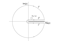
Figure 1: Contour used to evaluate $R_{\omega}^{0}$

Following the contour, as shown in Fig. 1, the contour integral can be expressed as

$$\oint d\rho~{}h(\rho)=I^{0}+I^{1}+I^{c}=(2\pi i)~{}\mathrm{Res}[h(\rho)]_{|\rho=1+i\epsilon}~{},$$ (37)

where $\mathrm{Res}[h(\rho)]_{|\rho=1+i\epsilon}$ is the residue of the function $h(\rho)$ evaluated at the pole $\rho=(1+i\epsilon)$. It can be easily shown that $I^{c}=0$ and $I^{1}=-e^{2\pi\omega/a}~{}I^{0}$. Therefore, the non-transient part of the transition rate can be expressed as

$$R_{\omega}^{0}=I^{0}=\frac{-(2\pi i)\mathrm{Res}[h(\rho)]_{|\rho=1+i\epsilon}}{e^{2\pi\omega/a}-1}~{}.$$ (38)

After taking the limit $\epsilon\to 0$, the evaluated residue at the pole of the two-point function in Fock space will be

$$\mathrm{Res}[h(\rho)]_{|\rho=1+i\epsilon}=\frac{i\omega}{2\pi}~{},$$ (39)

which leads the induced transition rate to become

$$R_{\omega}^{0}=\frac{\omega}{e^{2\pi\omega/a}-1}~{}.$$ (40)

This is the standard expression for mean energy per mode of a system in thermal equilibrium at the Unruh temperature $T=a/2\pi k_{B}$.

By considering reasonably large but finite time of observation, the transient part $\Delta R_{\omega}$ will be

$$\Delta R_{\omega}({\tau})\approx\frac{e^{-a\tau}}{\pi\left(1+\omega^{2}/a^{2}\right)}\left[a\cos(\omega\tau)-\omega\sin(\omega\tau)\right].$$ (41)

It clearly shows that the transient terms decay exponentially.

Therefore, if an Unruh-DeWitt detector is on for a sufficiently long time along a Rindler trajectory having magnitude of the acceleration 4-vector $a$, then Minkowski vacuum will appear as a thermal state at the temperature $T=a/2\pi k_{B}$.

VI Polymer quantization

In this section we discuss briefly about polymer quantization and then study Unruh effect numerically. In polymer quantization, the position operator $\hat{x}$ and translation operator $\hat{U}(\lambda)$ are considered as basic operators. In Polymer Hilbert space, the momentum operator does not exist as the translation operator is not weakly continuous in the parameter $\lambda$. However, one can define an analogous momentum operator as $\hat{p}_{\lambda}=1/(2i\lambda)(\hat{U}(\lambda)-\hat{U}(-\lambda))$, such that the usual momentum operator is recovered in the limit $\lambda\to 0$. In polymer quantization this limit does not exist and $\lambda$ is considered as a small and finite scale, $\lambda_{\star}$. This dimension-full parameter is analogous to Planck-length $L_{p}$ as $\lambda_{\star}\sim\sqrt{L_{p}}$.

The energy spectrum of the $\mathrm{k}-$th oscillator is Hossain et al. (2010)

$$\frac{E_{\mathrm{k}}^{2n}}{|\mathrm{k}|}=\frac{1}{4g}+\frac{g}{2}~{}A_{n}(g)~{},~{}\frac{E_{\mathrm{k}}^{2n+1}}{|\mathrm{k}|}=\frac{1}{4g}+\frac{g}{2}B_{n+1}(g)~{},$$ (42)

where $n\geq 0$, $A_{n}$, $B_{n}$ are Mathieu characteristic value functions and $g=|\mathrm{k}|{\lambda_{\star}}^{2}\equiv|\mathrm{k}|~{}l_{\star}$ is a dimension-less parameter. In terms of the cosine and sine elliptic functions Abramowitz and Stegun (1964) $\mathrm{ce}_{n}$ and $\mathrm{se}_{n}$, respectively, the energy eigenstates can be expressed as

$$\psi_{2n}(v) = \mathrm{ce}_{n}(1/4g^{2},v)/\sqrt{\pi},$$ (43)

$$\psi_{2n+1}(v) = \mathrm{se}_{n+1}(1/4g^{2},v)/\sqrt{\pi},$$

where $v=\pi_{\mathrm{k}}\sqrt{l_{\star}}+\pi/2$. Superselection rules are invoked to arrive at these $\pi$-periodic and $\pi$-antiperiodic states in $v$ Barbero G. et al. (2013).

For low-energy modes i.e., for small $g$, the energy spectrum (42) can be expressed as the energy spectrum of a regular harmonic oscillator along with perturbative corrections as

$$\frac{E_{\mathrm{k}}^{2n}}{|\mathrm{k}|}\approx\frac{E_{\mathrm{k}}^{2n+1}}{|\mathrm{k}|}\approx\left(n+\frac{1}{2}\right)+\mathcal{O}(g)~{}.$$ (44)

Therefore, one can recover the standard energy spectrum of the harmonic oscillator in the limit $g\to 0$. However, we should emphasize here that polymer energy spectrum has two-fold degeneracy as $g\to 0$ and it is lifted for finite values of $g$. The coefficients $b_{4n+3}=i\sqrt{l_{\star}}\int_{0}^{2\pi}\psi_{4n+3}\partial_{v}\psi_{0}dv$ are non-vanishing in polymer quantization for all $n=0,1,2,\ldots$, whereas in Fock quantization, only one $b_{n}$ is non-vanishing (32). Using asymptotic expressions of Mathieu functions, one can approximate the energy gaps $\Delta E_{n}$ between the levels and coefficients $b_{4n+3}$ for low-energy modes (sub-Planckian), $g\ll 1$,

$$\frac{\Delta E_{4n+3}}{|\mathrm{k}|}=(2n+1)-\frac{(4n+3)^{2}-1}{16}g+\mathcal{O}\left(g^{2}\right)~{},$$ (45)

for $n\geq 0$, and

$$b_{3}=\frac{i}{\sqrt{2|\mathrm{k}|}}\left[1+\mathcal{O}\left(g\right)\right]~{},~{}\frac{b_{4n+3}}{b_{3}}=\mathcal{O}\left(g^{n}\right),$$ (46)

for $n>0$. On the other hand, for high energy modes (super-Planckian), $g\gg 1$,

$$\frac{\Delta E_{4n+3}}{|\mathrm{k}|}=2(n+1)^{2}g+\mathcal{O}\left(\frac{1}{g^{3}}\right),$$ (47)

for $n\geq 0$, and

$$b_{3}=i\sqrt{\frac{g}{2|\mathrm{k}|}}\left[\frac{1}{4g^{2}}+\mathcal{O}\left(\frac{1}{g^{6}}\right)\right],\frac{b_{4n+3}}{b_{3}}=\mathcal{O}\left(\frac{1}{g^{2n}}\right),$$ (48)

for $n>0$. Therefore, in polymer quantization, we can approximate matrix element $D_{\mathrm{k}}(\Delta t)$ (29) by taking only the first element as

$$D_{\mathrm{k}}^{poly}(\Delta t)\simeq|b_{3}|^{2}e^{-i\Delta E_{3}\Delta t}~{},$$ (49)

for both the cases.

VI.1 Numerical computation of two-point function and Unruh effect

Using asymptotic expressions of the $b_{3}$ and $\Delta E_{3}$ one could analytically evaluate the two-point function for asymptotic spacetime intervals in polymer quantization. However, for all possible spacetime intervals it does not appear to be possible in polymer quantization, as in Fock quantization. In order to obtain a comprehensive picture of two-point function for all possible spacetime intervals we use numerical techniques.

VI.1.1 Matrix element $D_{\mathrm{k}}(\Delta t)$

The two-point function is completely understood from the matrix element $D_{k}(\Delta t)$, cf. equation (31). In polymer quantization, the matrix element (29) can be expressed as

$$D_{\mathrm{k}}^{poly}(\Delta t)=\sum_{n}|b_{4n+3}|^{2}e^{-i\Delta E_{4n+3}\Delta t},$$

$$= |b_{3}|^{2}e^{-i\Delta E_{3}\Delta t}\left[1+\frac{|b_{7}|^{2}}{|b_{3}|^{2}}e^{-i(\Delta E_{7}-\Delta E_{3})\Delta t}+\dots\right]~{}.$$

In Fock quantization, only the first term is non-vanishing. However, in polymer quantization there are infinitely many non-vanishing terms and from the asymptotic expressions (equations (46 and 48)) we can see that $b_{3}$ is larger than all other $b_{n}$ terms. Numerically we have shown that for the entire range of $g$, $|b_{7}|^{2}/|b_{3}|^{2}\ll 1$ (Fig. 2). It may also be shown that all other higher order coefficients are progressively smaller. Therefore, in order to simplify the numerical computation we restrict to the $b_{3}$ term only. For the purpose of comparison, we also plot the asymptotic expressions obtained from Eq. (45-48).

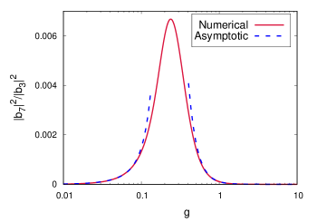
Figure 2: The solid red line represents numerically evaluated ratio between $|b_{7}|^{2}$ and $|b_{3}|^{2}$. The blue dashed line represents the same ratio using their respective asymptotic expressions.

VI.1.2 Coefficient $b_{k}$ and energy gap $\Delta E_{k}$

As discussed earlier, there is only one non-vanishing coefficient $b_{1}$ in Fock quantization which can be expressed in terms of dimensionless parameter $g$ as $|b_{k}|^{2}\equiv|b_{1}|^{2}=\frac{1}{2}(l_{\star}/g)$. For the purpose of comparison, we denote the coefficient $b_{3}$ as $b_{k}$ and the corresponding energy gap $\Delta E_{3}$ as $\Delta E_{k}$ also for polymer quantization. Figure 3 depicts $|b_{k}|^{2}$ as a function of $g$. The energy gap $\Delta E_{k}\equiv\Delta E_{3}=|\mathrm{k}|$ in Fock quantization and hence the ratio $\Delta E_{k}/|\mathrm{k}|$ is unity for all values of $g$. However, in polymer quantization, that ratio dips below unity and has a minima at $g\approx 0.26$. The behaviour of the energy gap $\Delta E_{k}$ as a function of $g$ is shown in Fig. 3.

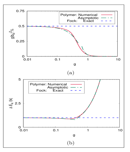
Figure 3: In Fock quantization, $g|b_{k}|^{2}/l_{\star}=\frac{1}{2}$ and is represented by the dashed blue line. The solid red line represents the numerical results and the dot dashed green line makes use of the asymptotic expressions for $|b_{k}|^{2}$ in polymer quantization. In Fock quantization, $\Delta E_{3}/|\mathrm{k}|=1$, which is represented by the blue dashed line. The solid red line represents the numerical results and the dot dashed green line represents asymptotic expressions for polymer quantization.

VI.1.3 Two-point function

In order to facilitate the numerical computation, we scale the two-point function as

$$G(\Delta t,\Delta\mathbf{x})=\frac{1}{4\pi^{2}l_{\star}^{2}}~{}\tilde{G}~{},$$ (51)

where $\tilde{G}$ is dimensionless. Taking into account the standard regulator $\epsilon$, and with the help of equations (30) and (31), the dimensionless two-point function can be expressed as

$$\tilde{G}^{\epsilon}=\int_{g_{min}}^{g_{max}}dg~{}\mathcal{T}(g,|\Delta\mathbf{x}|)~{}e^{-ip(g)-\epsilon g},$$ (52)

where $g_{min}$ and $g_{max}$ are limits of integration which are used to numerically represent $0$ and $\infty$, respectively. The above equation expresses the dimensionless two-point function on a uniform platform for both the Fock and polymer quantizations, respectively. The function $\mathcal{T}$ can be expressed in terms of dimensionless quantities as follows

$$\mathcal{T}(g,|\Delta\mathbf{x}|)=2~{}\left(\frac{|b_{k}|^{2}g}{l_{\star}}\right)~{}\left(\frac{l_{\star}}{|\Delta\mathbf{x}|}\right)~{}\sin\left(g\frac{|\Delta\mathbf{x}|}{l_{\star}}\right)~{}.$$ (53)

Similarly, the function $p(g)$ can also be expressed in terms of the dimensionless quantities as

$$p(g)=g~{}\left(\frac{\Delta E_{k}}{|\mathrm{k}|}\right)~{}\left(\frac{\Delta t}{l_{\star}}\right)~{}.$$ (54)

We should emphasize here that spacetime intervals $\Delta\mathbf{x}$ and $\Delta t$ are expressed in the units of $l_{\star}$.

In order to numerically compute the scaled two-point function $\tilde{G}$ (Eq. 52) in polymer quantization, we have used $g_{min}=10^{-3}$, $g_{max}=10^{3}$ and the integral regulator is taken to be zero, $i.e.~{},~{}\epsilon=0$. It should be noted here that a finite regulator is required in the Fock quantization in order to regulate the behavior of the two-point function. In contrast, in polymer quantization an inbuilt regulator precludes the need for an additional regulator.

We can see from the Fig. 4 that, for $\Delta t=0$, the scaled two-point function $\tilde{G}$ is real for all possible spatial intervals $\Delta\mathbf{x}$. On the other hand, for $\Delta\mathbf{x}=0$, $\tilde{G}$ has both real part (Fig. 5(a)) and imaginary part (Fig. 5(b)) for all possible temporal intervals $\Delta t$ . We also note here that unlike the Fock quantization, $\tilde{G}$ is bounded from above in polymer quantization and it converges to $\sim 0.21$ as both $\Delta t\to 0$ and $\Delta\mathbf{x}\to 0$. Analyzing these properties of $\tilde{G}$ and comparing with the standard form obtained from Fock quantization, we may conclude that in polymer quantization, there is an imaginary constant factor associated with $\Delta t$ which comes due to the standard “$i\epsilon$” regularization in Fock quantization. In polymer quantization this $\epsilon\approx 2.16$ whereas in Fock quantization, the limit $\epsilon\to 0$ is taken at the end of the computation. Therefore, in analogy with the Fock space two-point function, we can make an ansatz of the polymer two-point function as $\tilde{G}=1/[-(\Delta t-i~{}2.16)^{2}+|\Delta\mathbf{x}|^{2}]$.

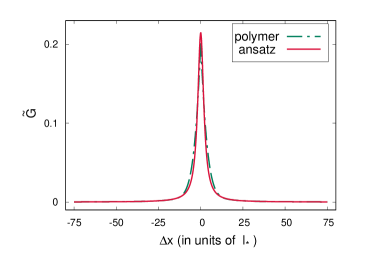
Figure 4: Figure depicts the scaled two-point function $\tilde{G}=4\pi^{2}l_{\star}^{2}G$ with respect to spatial intervals $\Delta\mathbf{x}$, when $\Delta t=0$. The dot dashed green and solid red line represents the result obtained from polymer quantization and from the ansatz respectively. In order to compute the polymer two-point function, we have taken the integral regulator $\epsilon=0$.

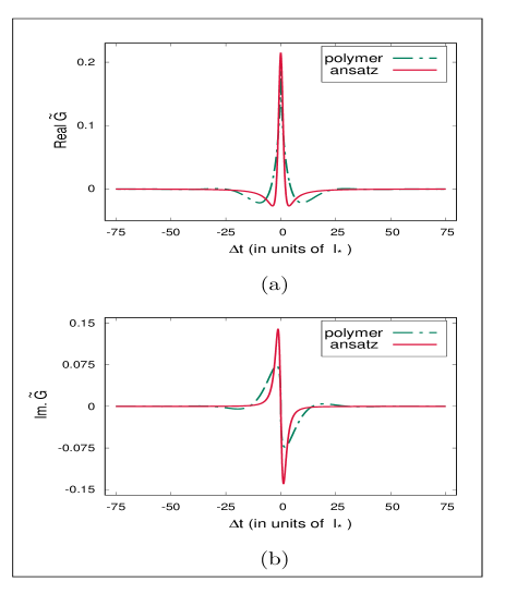
Figure 5: The sub-fig (a) represents the real-part and (b) represents the imaginary-part of the scaled two-point function $\tilde{G}=4\pi^{2}l_{\star}^{2}G$ with respect to temporal intervals $\Delta t$, when $\Delta\mathbf{x}\approx 0~{}(10^{-25})$. The dot dashed green and solid red lines represent the result obtained from polymer quantization and from the ansatz, respectively. In order to compute the polymer two-point function, we have taken the integral regulator $\epsilon=0$.

VI.1.4 Unruh effect

In order to numerically compute the transition rate of the Unruh-DeWitt detector along the Rindler trajectory $R_{\omega}(\tau,0)$ (Eq. 22), we have taken $a\tau=15$ and $a=1$ in the units of $l_{\star}^{-1}$ and the regulator is $\epsilon=0$ for polymer and $\epsilon=0.01$ for Fock quantization. The Fig. 6 exhibits the transition rate of the detector with a scaling $\tilde{R}$ with respect to $\tilde{\omega}=\omega/a$, where $\tilde{R}=(a/2\pi)R_{\omega}(\tau,0)$. We can see that in polymer quantization there is a non-thermal transition rate (dot dashed green line) which closely matches with the transition rate of the detector using the ansatz of the polymer-two-point function (red line). Therefore, we may conclude that the large value of the regulator $\epsilon\approx 2.16$ plays a crucial role for the non-thermal transition rate. We should emphasize here that the transition rate obtained from the polymer quantization has large deviations from the thermal spectrum obtained from Fock quantization (dashed blue line) at lower $\tilde{\omega}$ which implies higher acceleration $a$. This suggests that very high acceleration (comparable to Planck-length scale) would be needed to probe the Planck-length scale effect on the Unruh effect. It would be pertinent to note that the value of the regulator $\epsilon\approx 2.16$ does not depend on the polymer length scale. Hence, a generic cut-off is seen to emerge in polymer quantization, a feature that could be probed by experiments on the Unruh effect Nation et al. (2012); Aspachs et al. (2010).

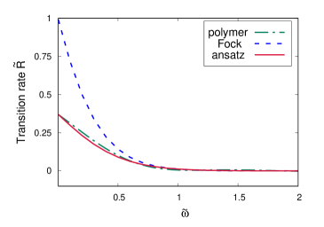
Figure 6: The transition rate of the Unruh-DeWitt detector along the Rindler trajectory, where $al_{\star}=1$. The dot dashed green, dashed blue and solid red lines represent the results obtained from polymer quantization, Fock quantization and ansatz, respectively. In order to compute the transition rate we have taken the integral regulator $\epsilon=0$ for polymer and $\epsilon=0.01$ for Fock quantization.

VII spatially smeared detector and “$i\epsilon$” regularization

Up to this point our study of the Unruh effect involves a point-like detector. In order to regularize the two-point function, the standard “$i\epsilon$” regularization technique is used in Fock quantization. However, there is an issue with Lorentz invariance and it can be taken care of by considering a spatially smeared detector for which the field operator will be

$$\hat{\Phi}(\tau)=\int d^{3}\chi~{}f(\chi)\hat{\Phi}(x(\tau,\chi)),$$ (55)

where $\tau$ and $\chi$ are the Fermi-Walker coordinates which are associated with the trajectory $x(\tau)$, and $f(\chi)$ is the spatial profile of the detector. If the spatial profile of the detector is taken as Schlicht (2004)

$$f_{\delta}(\chi)=\frac{1}{\pi^{2}}\frac{\delta}{(\chi^{2}+\delta^{2})^{2}}~{},~{}\delta>0,$$ (56)

then the two-point function in Fock quantization becomes

$$G(x(\tau),x(\tau^{\prime}))=\frac{1/4\pi^{2}}{(x(\tau)-x(\tau^{\prime})-i\delta(\dot{x}(\tau)+\dot{x}(\tau^{\prime})))^{2}}~{}.$$ (57)

We have numerically computed the transition rate of the detector considering both spatially smeared detector and point-like detector where “$i\epsilon$” regularization is used. It can be seen from Fig. 7 (a) that the transition rate is much more insensitive to the detector size regulator $\delta$ than the standard regulator $\epsilon$. Fig. 8 depicts the transition rate of the detector, in polymer quantization. It can be seen that the transition rate is similar for small values of the detector size $\delta$ and $\epsilon$ regulators, $\delta=0.01,\epsilon=0.0$ and $\delta=0.0,\epsilon=0.01$, respectively for both quantization methods.

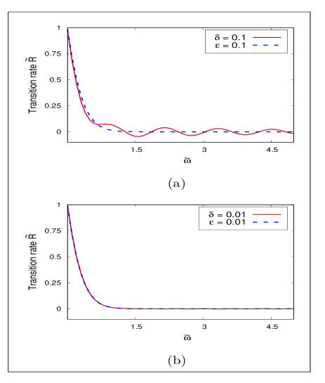
Figure 7: Transition rate of the Unruh-DeWitt detector along the Rindler trajectory in Fock quantization, where $al_{\star}=1$. The solid red line and dashed blue line represents the transition rate for different detector size regulator $\delta$ and the regulator $\epsilon$, respectively. The sub-fig (a) represents detector size and $\epsilon$ regulator $\delta=0.1$, $\epsilon=0$; $\delta=0,~{}\epsilon=0.1$ and the sub-fig (b) represents detector size and $\epsilon$ regulator $\delta=0.01$, $\epsilon=0$; $\delta=0,~{}\epsilon=0.01$.

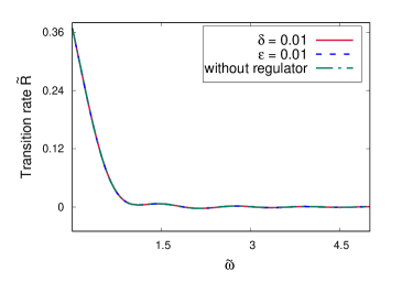
Figure 8: Transition Rate of the Unruh-DeWitt detector along the Rindler trajectory in polymer quantization, where $al_{\star}=1$. The solid red, dashed blue and dot dashed green lines represent the results obtained from polymer quantization with the detector size and $\epsilon$ regulators $\delta=0.01$, $\epsilon=0$; $\delta=0$, $\epsilon=0.01$ and $\delta=\epsilon=0$, respectively.

VIII Discussions

To summarize, we have studied the transition rate of a uniformly accelerated Unruh-DeWitt detector weakly coupled to a massless scalar field for both the Fock as well as polymer quantizations. An essential ingredient for computing the transition rate of the detector is the two-point function along the detector’s trajectory. For the case of polymer quantization, this is accomplished numerically. By comparing the numerically computed polymer and Fock space two-point functions, it is observed that the the regulator $\epsilon$ which is used for the standard regularization for Fock space two-point function is generic in the case of polymer-two-point function with a finite value $\epsilon\approx 2.16$. Thus, a generic cut-off is seen to emerge in polymer quantization, a feature that could be probed by experiments on the Unruh effect.

Subsequently, the transition rate of the accelerated detector has been computed. This rate is non-thermal in polymer quantization, for high detector acceleration and closely matches with the transition rate using the ansatz of the polymer two-point function, $i.e.$ , the Fock space two-point function with the regulator value $\epsilon\approx 2.16$. Therefore, it follows that the large value of the regulator $\epsilon\approx 2.16$ leads to deviation from the thermal spectrum, as obtained from the Fock quantization. The deviation increases as the acceleration $a$ increases. This suggests that in order to probe Planck scale effect on Unruh effect one needs to have a large acceleration. We would like to emphasize here that the value of the regulator $\epsilon\approx 2.16$ does not depend on the polymer length scale.

Finally, we have also discussed the role of a spatially smeared detector on the transition rate. It can be seen that the transition rate is more sensitive to the detector size $\delta$ than the standard regulator $\epsilon$. However, for small value of the $\delta$ and $\epsilon$, the transition rate is similar for both quantization methods.

References

- Fulling (1973) S. A. Fulling, Phys.Rev. D7, 2850 (1973).
- Unruh (1976) W. Unruh, Phys.Rev. D14, 870 (1976).
- Crispino et al. (2008) L. C. Crispino, A. Higuchi, and G. E. Matsas, Rev.Mod.Phys. 80, 787 (2008), eprint arXiv:0710.5373.
- De Bièvre and Merkli (2006) S. De Bièvre and M. Merkli, Classical and Quantum Gravity 23, 6525 (2006).
- Takagi (1986) S. Takagi, Progress of Theoretical Physics Supplement 88, 1 (1986).
- Longhi and Soldati (2011) P. Longhi and R. Soldati, Phys.Rev. D83, 107701 (2011), eprint arXiv:1101.5976.
- Davies (1975) P. C. W. Davies, J. Phys. A8, 609 (1975).
- Birrell and Davies (1984) N. D. Birrell and P. C. W. Davies, Quantum fields in curved space, 7 (Cambridge university press, 1984).
- Banerjee et al. (2016) S. Banerjee, A. K. Alok, and S. Omkar, Eur. Phys. J. C76, 437 (2016), eprint arXiv:1511.03029.
- Omkar et al. (2016) S. Omkar, S. Banerjee, R. Srikanth, and A. K. Alok, Quant. Inf. Comput. 16, 0757 (2016), eprint arXiv:1408.1477.
- Banerjee et al. (2017) S. Banerjee, A. K. Alok, S. Omkar, and R. Srikanth, JHEP 02, 082 (2017), eprint arXiv:1603.05450.
- Nicolini and Rinaldi (2011) P. Nicolini and M. Rinaldi, Phys.Lett. B695, 303 (2011), eprint arXiv:0910.2860.
- Padmanabhan (2010) T. Padmanabhan, Rept.Prog.Phys. 73, 046901 (2010), eprint arXiv:0911.5004.
- Agullo et al. (2008) I. Agullo, J. Navarro-Salas, G. J. Olmo, and L. Parker, Phys.Rev. D77, 124032 (2008), eprint arXiv:0804.0513.
- Chiou (2018) D.-W. Chiou, Phys. Rev. D97, 124028 (2018), eprint arXiv:1605.06656.
- Alkofer et al. (2016) N. Alkofer, G. D’Odorico, F. Saueressig, and F. Versteegen, Phys. Rev. D94, 104055 (2016), eprint arXiv:1605.08015.
- DeWitt (1980) B. S. DeWitt, in General Relativity: An Einstein Centenary Survey (1980), pp. 680–745.
- Hinton (1983) K. J. Hinton, Journal of Physics A: Mathematical and General 16, 1937 (1983).
- Schlicht (2004) S. Schlicht, Class. Quant. Grav. 21, 4647 (2004), eprint gr-qc/0306022.
- Louko and Satz (2006) J. Louko and A. Satz, Class. Quant. Grav. 23, 6321 (2006), eprint gr-qc/0606067.
- Unruh and Wald (1984) W. G. Unruh and R. M. Wald, Phys. Rev. D29, 1047 (1984).
- Louko (2014) J. Louko, JHEP 09, 142 (2014), eprint arXiv:1407.6299.
- Sriramkumar and Padmanabhan (1996) L. Sriramkumar and T. Padmanabhan, Class. Quant. Grav. 13, 2061 (1996), eprint gr-qc/9408037.
- Agullo et al. (2010) I. Agullo, J. Navarro-Salas, G. J. Olmo, and L. Parker, New J. Phys. 12, 095017 (2010), eprint arXiv:1010.4004.
- Fewster et al. (2015) C. J. Fewster, B. A. Juárez-Aubry, and J. Louko, in 14th Marcel Grossmann Meeting on Recent Developments in Theoretical and Experimental General Relativity, Astrophysics, and Relativistic Field Theories (MG14) Rome, Italy, July 12-18, 2015 (2015), eprint arXiv:1511.00701.
- Satz (2007) A. Satz, Class. Quant. Grav. 24, 1719 (2007), eprint gr-qc/0611067.
- Langlois (2006) P. Langlois, Annals Phys. 321, 2027 (2006), eprint gr-qc/0510049.
- Hümmer et al. (2016) D. Hümmer, E. Martin-Martinez, and A. Kempf, Phys. Rev. D93, 024019 (2016), eprint arXiv:1506.02046.
- Ashtekar et al. (2003) A. Ashtekar, S. Fairhurst, and J. L. Willis, Class.Quant.Grav. 20, 1031 (2003), eprint gr-qc/0207106.
- Halvorson (2004) H. Halvorson, Studies in history and philosophy of modern physics 35, 45 (2004).
- Ashtekar and Lewandowski (2004) A. Ashtekar and J. Lewandowski, Class.Quant.Grav. 21, R53 (2004), eprint gr-qc/0404018.
- Rovelli (2004) C. Rovelli, Quantum Gravity, Cambridge Monographs on Mathematical Physics (Cambridge University Press, 2004), ISBN 9780521837330.
- Thiemann (2007) T. Thiemann, Modern Canonical Quantum General Relativity, Cambridge Monographs on Mathematical Physics (Cambridge University Press, 2007), ISBN 9781139467599.
- Rindler (1966) W. Rindler, Am.J.Phys. 34, 1174 (1966).
- Hossain et al. (2010) G. M. Hossain, V. Husain, and S. S. Seahra, Phys.Rev. D82, 124032 (2010), eprint arXiv:1007.5500.
- Abramowitz and Stegun (1964) M. Abramowitz and I. Stegun, Handbook of Mathematical Functions: With Formulas, Graphs, and Mathematical Tables, Applied mathematics series (Dover Publications, 1964), ISBN 9780486612720.
- Barbero G. et al. (2013) J. F. Barbero G., J. Prieto, and E. J. Villaseñor, Class.Quant.Grav. 30, 165011 (2013), eprint arXiv:1305.5406.
- Nation et al. (2012) P. D. Nation, J. R. Johansson, M. P. Blencowe, and F. Nori, Rev. Mod. Phys. 84, 1 (2012), eprint arXiv:1103.0835.
- Aspachs et al. (2010) M. Aspachs, G. Adesso, and I. Fuentes, Phys. Rev. Lett. 105, 151301 (2010), eprint arXiv:1007.0389.